Technical note: A framework for causal inference applied to solar radiation and temperature effects on measured levels of gaseous elemental mercury in seawater

Environmental science usually requires researchers to rely on observational data alone. However, researchers want to identify causal relationships and not only correlations between pollutant behaviour and other environmental factors such as weather. Previously it has been shown that solar radiation associates with the volatilisation and evasion of the hazardous pollutant mercury from sea surfaces into the atmosphere. Statistical and machine learning methods can help find and quantify such associations. However, association does not imply causation, and inferring causal relationships from observational data alone remains a significant challenge. Here, we aim to create an “easy-to-follow” framework, to be used by environmental researchers, for using prior scientific knowledge encoded as graphical causal models to enable causal inference and to estimate effect sizes of different related factors using collected field data. We demonstrate the framework through a case study estimating the effect sizes of solar radiation and sea surface temperature on levels of gaseous elemental mercury (C_MW) in seawater measured at the west coast of Sweden. Our causal analysis reveals that 32 % of the total effect of solar radiation on (C_MW) is mediated indirectly via changes in sea surface temperature. Wind and instrumentation intrinsic factors biased the estimates by 4.5 %. Results from the case study show that our proposed framework allows for a rigorous design, validation, and reporting of causal inference in environmental science. The framework shows potential in modelling causes of pollutant dynamics and quantifying the effect of regulating policies such as the Minamata Convention on Mercury.

1 Introduction

Environmental, and particularly atmospheric monitoring and research, rely on direct measurements and modelling to understand the processes involved in the formation, transport, evasion, and deposition of different pollutants. The purpose of environmental monitoring is often defined and driven by national and international legislations and directives, defined within the European Union (European Parliament and Council, 2004), or through international conventions such as the United Nations Framework Convention on Climate Change (United Nations, 1992) and the Convention on Long-Range Transboundary Air Pollution CLRTAP (United Nations Economic Commission for Europe, 2024; United Nations, 1979). Depending on legislative and pollutant, the requirements for monitoring could include either modelling, estimations, or direct and continuous measurements with yearly reporting to co-operative programs under CLRTAP, e.g., the European Monitoring and Evaluation Programme (EMEP, 2023). For mercury, directive 2004/107/EG describes the need of ensuring collecting publicly available information about concentrations in air and deposition in every member state of the European Union (European Parliament and Council, 2004). The directive further demands that indicative measurements of mercury shall be performed at background sites at a spatial resolution of 100 000 km². Within the United Nations, a global convention, aimed to protect human health and the environment from the exposure of mercury, was agreed on in January 2013 and was named the Minamata Convention on Mercury (United Nations Environment Programme, 2024). The convention entered into force in August 2017 and is today ratified by more than 150 parties all over the world. At present, an Effectiveness Evaluation Group has been selected to assess the effectiveness of the convention by studying trends and changes in mercury concentrations in different media (United Nations Environment Programme, 2024).

This leads to another aspect of environmental monitoring: the use of computer models to analyse and interpret complex environmental data to make predictions about unseen or future data points, to understand patterns and trends, and to evaluate the effectiveness of current legislatives. Learning about the dependencies between variables from observational data allows us to build predictors that provide necessary estimates of previously unseen data. These predictors are statistical learning machines, which can take the form of simple regression models or even highly complex and opaque ML models such as convolutional neural networks (CNNs). However, environmental researchers are not only interested in building opaque, black-box prediction machines that magically predict future data points from observational data. Instead, they are particularly interested in understanding cause-effect relationships to suggest interventions that reduce pollutants in the environment. Causal knowledge, or in other words the analysis of cause-effect relationships, is one of the “fundamental goals of science” (Vowels et al., 2022; Rose and van der Laan, 2011).

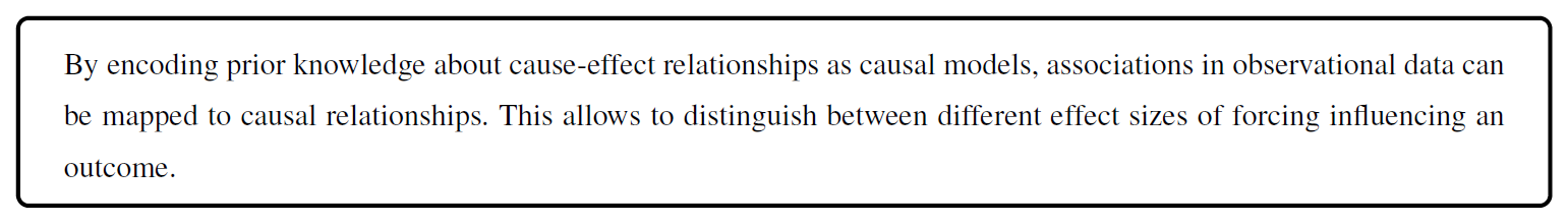
Pearl et al. (2016) highlight that causal questions, i.e., question about what are causes and effects, usually cannot be answered from observational data alone. Instead, additional assumptions are needed that specify an assumed causal structure underlying the data-generating process. Causal inference from observational data is therefore not assumption-free. Its conclusions depend on the correctness and completeness of the prior knowledge represented as graphical causal model. Accordingly, the framework presented in this paper does not aim to discover causal structure from data alone, nor does it aim to provide a definitive proof of causation. Instead, its scope is to offer a transparent and principled way to reason about causal effect sizes using observational environmental data and prior knowledge, and to assess the compatibility of that prior knowledge with the observed data. By making prior knowledge and assumptions about cause-and-effect relationships explicit as graphical models, causal conclusions drawn from observational data can be scrutinised, criticised, and revised.

This paper reports the results of a case study on extracting causal knowledge about the contribution of different environmental processes to the observed levels of gaseous elemental mercury (C_MW) in seawater. Although measurements of gaseous mercury in water is not yet a requirement within any EU directive, the results from novel continuous measurements of mercury (Hg) in surface water are used as a case study. This paper proposes a framework for obtaining and reporting causal knowledge from environmental observational data. Through the case study, this paper explains how to build statistical models that not only predict future values of an outcome variable but also allow the inference of causal relationships between predictor variables and the outcome using observational data.

1.1 Environmental monitoring of mercury emissions

Mercury is considered by the World Health Organization to be one of the top ten chemicals or substances to be of major concern to public health (Cohen et al., 2005). This volatile and toxic element is found naturally in various environmental compartments and originates from both natural and anthropogenic sources, such as artisanal small scale gold mining, burning of fossil fuels and various industrial activities. As a gas, mercury is stable and has a long residence time in air, resulting in a global spread via the atmosphere to remote, pristine, and vulnerable environments such as the polar regions. Mercury is deposited from air by dry and wet deposition, often via oxidation from Hg⁰ to Hg^II. Oxidised mercury in seawater, for example, transforms more easily into methylmercury which can bioaccumulate in aquatic food chains. However, it can also reduce back to its elemental form and evade back to the atmosphere, where it is capable of fast long-range transport. Mercury evasion from sea surfaces accounts for almost 50 % of the annual contributions to the atmospheric mercury load. This is because much of the oceans' surfaces are supersaturated with elemental mercury compared to the atmosphere, resulting in net water-to-air evasion (AMAP, 2021). Understanding the drivers behind formation of dissolved gaseous mercury (DGM) and subsequent flux is key to understand the bioavailability of methylmercury in seawater and supporting global models with information about spatial and temporal variability (Soerensen et al., 2013). Mercury flux models for seawater suggest that the flux, and thus the fluctuation of DGM concentration in surface waters, is mostly influenced by environmental factors such as wind speed, temperature, photochemistry and microbial activity (Soerensen et al., 2013; Johnson, 2010; Kuss et al., 2009). What controls the formation of DGM is also debated, and it is discussed that it is formed by demethylation processes of methyl- and dimethylmercury in the subsurface ocean (Munson et al., 2018). Demethylation could be either abiotic or biotic, with an abiotic process being photo-demethylation controlled by solar radiation (AMAP, 2021). The connection between the formation of DGM and solar radiation has previously been studied in various environmental compartments such as the sea, lakes, soils, and salt marshes (Xie et al., 2019; Sizmur et al., 2017; Dill et al., 2006; Gårdfeldt et al., 2001; Amyot et al., 1997). In several studies, the relationship between DGM and solar radiation was quantified by determining correlation coefficients of 0.66 (Cane Creek Lake, USA; Dill et al., 2006), 0.99 (river near Knobesholm, Sweden; Gårdfeldt et al., 2001), and 0.39 (coastal Minamata Bay, Japan; Marumoto and Imai, 2015), suggesting that solar radiation can be an important, though site-dependent, predictor of DGM. Other studies report similar relationships between mercury evasion and solar radiation with correlation coefficients of 0.7, (Adriatic Sea; Floreani et al., 2019) and 0.5–0.9 (Wuijang River, China; Fu et al., 2013). However, there is probably more to the story of how the concentration of DGM is influenced by external factors such as solar radiation. Sizmur et al. (2017) hypothesised that the formation of DGM probably is affected by a combination of solar radiation and increased temperature. Zhang et al. (2006) performed a Pearson analysis of DGM and various factors measured at Lake St. Pierre (Canada), including air and water temperature, wind speed and solar radiation. The analysis showed significant correlations between DGM and all of these factors. Other aspects, such as water depth, have also been shown to have an effect on how strong the influence of solar radiation is for the formation of DGM in surface seawater, since the correlation mainly has been observed at the coast (Nerentorp Mastromonaco et al., 2017; Fantozzi et al., 2013; Ferrara et al., 2003; Lanzillotta et al., 2002; Andersson et al., 2007). The reason has been suggested to be due to greater vertical and turbulence mixing (Nerentorp Mastromonaco et al., 2017; Lanzillotta et al., 2002), lower friction velocities and surface roughness (Fantozzi et al., 2013), and the presence of dissolved organic carbon (DOC) and suspended particles (Ferrara et al., 2003; Amyot et al., 1997).

In summary, we see that merely calculating and discussing correlations will not capture the underlying causal mechanisms by which different environmental forcings influence DGM. What is needed instead is an approach that can separate correlation from causation while also accounting for cause–effect relationships among the forcings themselves, such as solar radiation influencing temperature.

1.2 Outline and purpose of the paper

The intention of this paper is to provide a discussion of the role of graphical causal models in environmental research and to present suggestions on how effect sizes from observational data in environmental science can be systematically obtained and reported.

In Sect. 2, the paper describes the used case study of continuous measurements of gaseous elemental Hg (C_MW) and calculated DGM in seawater, carried out on the west coast of Sweden in 2020. Section 3 introduces a framework for causal inference using observational data. Section 4 then describes how the proposed framework for causal inference is applied to the case data for inferring the effect sizes of different forcing, such as solar radiation, sea surface temperature, wind speed, and speed of the instrument feeding water pump on measured Hg concentrations C_MW. Section 5 presents the results from the case study and in Sect. 6 these results and the application of the framework for causal inference using observational environmental data are discussed, leading to concluding remarks and suggestions for further research presented in Sect. 7.

2 Description of case study: Continuous measurements of Hg concentration in seawater

The measurement campaign was conducted between 5 December 2019 and 8 October 2020 at the Kristineberg Marine Research Station, located on the Swedish West-coast (58.25013° N, 11.44485° E). Kristineberg is located at the entry of the Gullmarsfjord in the Skagerrak Sea which is classified as a natural reserve. With its shallow waters it serves as an important reproduction site for shellfish. The data for this study were collected during the period 1 to 25 April 2020, which is an interesting time period for our case study due to the good mixture between dark and sunlit hours in Scandinavia at this time of the year. All data are presented in Table 3 and Fig. 6 in Sect. 5.1.

2.1 Measurements of Hg concentration in surface water

Measuring DGM in water is commonly performed by manually collecting a water sample which is purged using an inert gas, resulting in that gaseous Hg is released and pre-concentrated on an adsorbent trap (typically gold), which is anlalysed with thermal desorption and detection using cold vapour atomic flourescence spectrometry (CVAFS) or cold vapour atomic absorption spectrometry (CVAAS). With manual sampling, DGM is easily calculated by dividing the total amount of Hg captured on the adsorbant trap with the sample volume (Gårdfeldt et al., 2002; Andersson et al., 2008a). However, continuous sampling is often preferable to increase time resolution which is needed for studying the dynamics of DGM in surface waters. Continuous sampling methods are normally divided by two different approaches; one where the aim is to extract all Hg from the continuous inflow of water and a second approach which aims to establish an equilibrium between Hg in the water phase and the gas phase. In the second approach, which is used in this study, the DGM concentration is normally recalculated by dividing the measured Hg concentration in outgoing air by the dimensionless Henry´s law constant that describes the partitioning of mercury between the gaseous and aqueous phase. Henry's law constant for mercury in seawater has previously been determined by Andersson et al. (2008b) to be temperature dependent and is calculated as

$$\begin{array}{}\text{(1)}& H^{\prime }=e^{(-\mathrm{2404.3}/T(K\left)\right)+\mathrm{6.92}}.\end{array}$$

The automatic continuous equilibrium system used in this study, developed by Andersson et al. (2008a) and further used in e.g., Nerentorp Mastromonaco et al. (2017) and in Osterwalder et al. (2020), consist of an inner cylinder in which incoming seawater enters continuously from the top, see Fig. 1b. A purging system, consisting of a glass frit, was installed at the bottom of the inner cylinder. The air used for purging was pumped using an air pump. A massflow controller regulated the air flow (r_a) to a fixated 1.5 L min⁻¹. Ambient air normally contains small amount of Hg (c_a0 in Fig. 1b), but in our set-up, a coal canister was used to remove Hg from the purging air. After purging through the water in the inner cylinder, the air outflow, now containing the equilibrium concentration of extracted gaseous mercury (C_MW), was first led through a soda lime trap and a polytetrafluoroethylene (PTFE, 2 µm pore size, 47 mm diameter) filter to prevent particles and moisture from entering the analyser. The purged sea water flowed out via the bottom of the inner cylinder, moving upwards inside the outer cylinder and was then discharged back to the sea via a rubber tubing. The purpose of the backflow system using an outer cylinder is to serve as isolation to keep the temperature in the inner cylinder as stable as possible during purging. All small tubing in the system was made of FEP (fluorinated ethylene propylene).

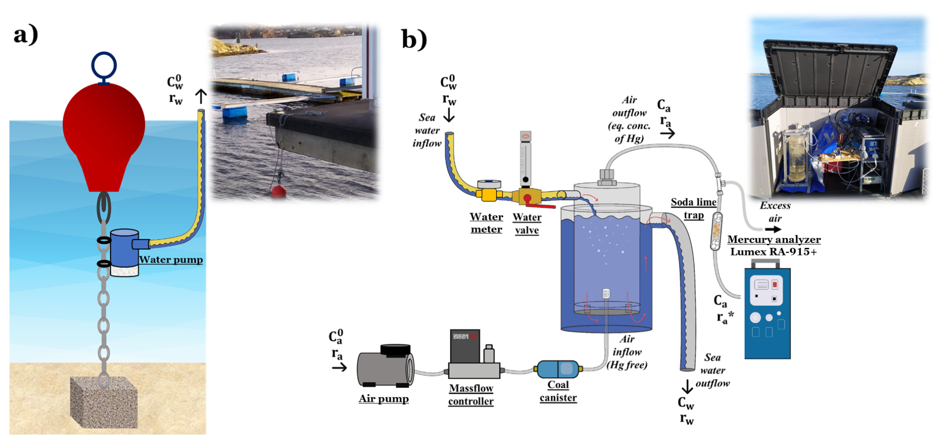
Figure 1 Experimental set-up for measuring gaseous mercury in surface water: (a) sampling site consisting of a red buoy which holds up a chain that is attached to the bottom with an anchor. The water pump is fixated on the chain about 1 m below the buoy; (b) measurement site containing the continuous equilibrium system for extracting gaseous mercury from seawater and the Lumex RA-914+ mercury analyser.

Finally, the equilibrium concentration of extracted gaseous elemental mercury (C_MW) in the air outflow was analysed every minute using a Lumex RA-914+ CVAAS. Calibration of the instrument was performed automatically every three hours by adjusting the baseline using mercury free air. The detection limit of the instrument has previously been determined to be 0.5 ng m⁻³, having a precision of ±5 % (Nerentorp Mastromonaco et al., 2017). The blank of the automated continuous equilibrium system was determined by turning off the water pump, letting water within the system be depleted of gaseous Hg. The detection limit of the system was determined to 0.32 pg L⁻¹, calculated as three times the standard deviation of the blanks.

C_MW measured with the analyser can be used to calculate the concentration of dissolved gaseous mercury (DGM) in incoming seawater. If C_a0 is removed from Hg, the equation to calculate DGM can be simplified to (Andersson et al., 2008a; Gårdfeldt et al., 2002):

$$\begin{array}{}\text{(2)}& \text{DGM}=C_{\mathrm{MW}}\left({\displaystyle \frac{\mathrm{1}}{H^{\prime }}}+{\displaystyle \frac{r_{\mathrm{A}}}{r_{\mathrm{w}}}}\right),\end{array}$$

where C_MW is the measured Hg concentration in the air outflow from the purging system (pg L⁻¹), H^′ is the dimensionless Henry's law constant that describes the partitioning of mercury between the gaseous and aqueous phase. The variables r_A and r_w denote the flow rates of purging air and seawater (L min⁻¹), respectively. When studying Eqs. (1) and (2) it becomes clear that sea water temperature is already integrated into the calculation of DGM, which can cause uncontrollable feedback loops when studying direct effects between DGM and sea surface temperature in our model. To avoid this problem, C_MW was chosen as a outcome variable instead of DGM in this study. Calculated DGM concentrations, which in this study only are presented for comparison, are presented in Table 3 and Fig. 6f in Sect. 5.1.

The measurements were conducted in shallow waters (< 10 m depth) at the harbour of Kristineberg. At the sampling site, a commercial 12 V bilge pump¹ with the capacity to pump 32 L min⁻¹ was installed on a chain, attached to a buoy and an anchor, at 1 m below the buoy to keep the same water depth to the surface, disregarding tide or waves, see Fig. 1a. A cage of fine mesh net was installed around the pump to reduce pump clogging problems due to algal growth (not shown in Fig. 1a). The seawater was pumped from the sampling site to the measurement site through a rubber tubing, lying on the bottom of the sea. The distance between the sampling site and the measurement site was less than 10 m. At the measurement site (Fig. 1b), a plastic cabinet shielded the equipment from weather and sun. A temperature controlled radiator inside the cabinet kept the equipment at a constant temperature. The flow of incoming seawater from the measuring site was measured and controlled using a water meter and a valve. The regulated water flow in Fig. 1 is denoted r_W. A constant water flow was hard to obtain due to the pump experienced problems with growth of algae and clogging, despite installing a protective net. During April 2020, r_w varied between 0 and 40 L min⁻¹, with an average flow rate of 2.8 L min⁻¹, see Table 3 and Fig. 6e in Sect. 5.1.

2.2 Measurements of solar radiation and surface water temperature

Solar radiation, denoted as Sol, was measured using a pyranometer sensor from Renke, model RS-TBQ measuring both direct and diffuse solar irradiance with a measurement range of 0–2000 W m⁻², a resolution of 1 W m⁻² and an accuracy of ±3 %. The sensor was installed on the roof of the measurement box, having no shadowing. The output of the sensor was read by an Arduino embedded computer which transformed the output voltage into irradiance in W m⁻² and sent the result to a central computer for logging alongside the other measurements. The temperature of the incoming seawater was measured at the inlet to the automated continuous equilibrium system using a DS18B20 temperature probe connected and processed by the same Arduino embedded computer.

Other weather data, such as wind speed, were downloaded from a weather station situated in the Gullmarsfjord close to the research station. These measurements are run by the University of Gothenburg and are available online (University of Gothenburg, 2024).

All variables have been resampled to 5 min intervals using a moving average filter. This has been done for two reasons: firstly, we did not suspect that the dynamics of the observed effects are faster than 10 min, which is twice the new sampling rate and therefore fulfils the Nyquist–Shannon sampling theorem. Secondly, we reduced the amount of datapoints which allowed for faster processing in the modelling steps. The measurements of solar radiation, seawater temperature and wind speed are presented in Table 3 and Fig. 6a, b and d, respectively.

3 A framework for causal inference using observational data in environmental research

The workflow to estimate effect sizes in this study is presented as a framework for researchers conducting causal inference from observational data. It builds on existing causal inference workflows proposed in behavioural science (Deffner et al., 2022) and software engineering (Furia et al., 2024). However, unlike these domains, environmental research relies to a much higher degree on data from intervention-free observational studies, motivating a tailored framework for causal inference using observational environmental data and prior scientific knowledge from researchers. Here, causal relationships are not discovered from the observational data itself, but are assumed based on prior experimental and scientific knowledge, such as laboratory studies demonstrating photochemical DGM production under controlled conditions. The scope of the proposed framework is then to quantify how multiple established or assumed causal processes jointly contribute to observed variability under natural, intervention-free field conditions. Using causal models, as suggested in this framework, conceptually allows individual causal pathways to be “switched off” within the model. This allows assessing the causal pathways' relative contribution without the need to physically intervene in the environmental system, which often is impossible in field observation.

Box 1 A framework for causal inference using observational data in environmental research.

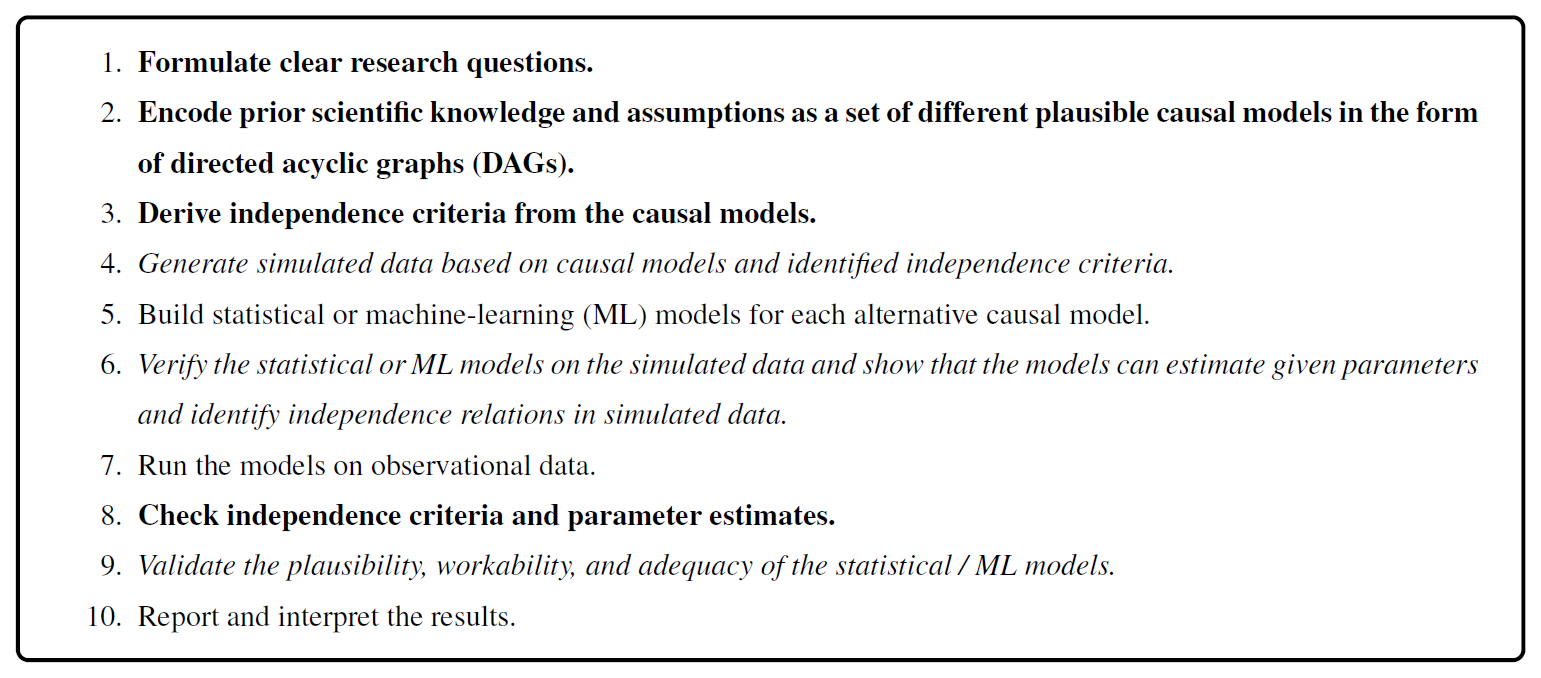
The proposed framework consists of ten steps which can be divided into three groups: steps for incorporating and testing prior knowledge (steps 1, 2, 3, and 8), steps for collecting evidence of plausibility, workability, and adequacy (steps 4, 6, and 9), and steps for generating answers to research questions (steps 5, 7, and 10). The steps are interlinked, which suggests an order in which we propose to execute them as shown in Fig. 2.

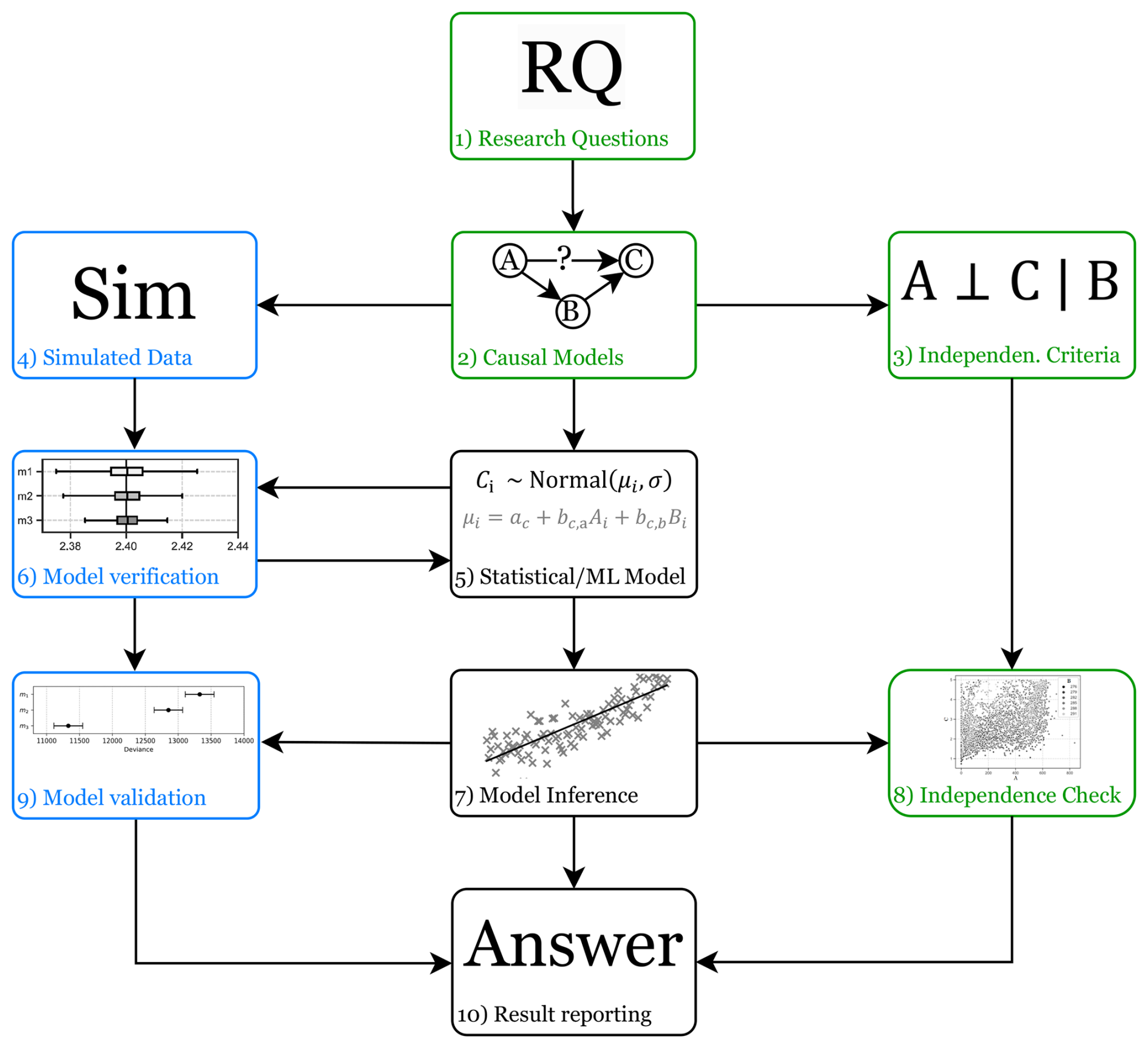
Figure 2 A workflow for causal inference of statistical models using observational data and prior knowledge about plausible cause-effect relationships.

In steps 1–3, research questions are formulated, and prior scientific knowledge and assumptions are encoded in a set of possible graphical causal models. A causal model describes “relevant features of the world and how they interact with each other” (Pearl et al., 2016). Which features are relevant depends on the research questions and scope of the investigation. A causal model indicates how a change in one variable changes the value of another variable, regardless of the functional form of the relationship. Causal models include two types of variables. The first type, exogenous variables, are not explained further within the model. For example, solar radiation Sol affects ocean surface temperature T_S (Sol → T_S). Here, we treat Sol as an exogenous variable without modelling upstream mechanisms such as the sun’s fusion reactions. The second type, endogenous variables, by contrast, are always descendants of at least one exogenous variable. Directed Acyclic Graphs (DAGs) provide an accessible visualisation of causal models with nodes representing the variables of a system of interest and directed edges representing the direction of cause-and-effect. The causal model of the earlier example Sol → T_S is in the form of a DAG, with the arrow → indicating that solar radiation is a cause of changes in surface temperature, and not the other way around. Note that in this framework, causal arrows are not inferred from data but represent a priori assumptions about cause-effect directions derived from domain knowledge or experimental evidence. The graphical representation of causal models through DAGs is qualitative, i.e., it provides information about the direction of cause-and-effects between variables, but it does not provide information about the strength or functional properties of the causal relationships. Causal inference, as proposed in this framework, provides the quantification of effect sizes and it evaluates whether the observational data is consistent with the assumed qualitative causal structure. Pearce and Lawlor (2016) provide an overview of properties of DAGs representing causal models:

• DAGs are directed, i.e., the arrows can only have a single head pointing from the cause towards the effect.

• DAGs are acyclic, meaning that there must not be a series of arrows (i.e., a path) resulting in a cyclic path. Causal models are acyclic because a variable at a given point in time cannot be the cause of itself.

• An arrow indicates that (we assume) a causal relationship exists between two variables, where the first variable has an effect on the second variable.

• The absence of an arrow indicates that the values of two variables are not causally related, i.e., a change in the value of one variable has no effect on the value of the second variable.

• The outcome variable is typically an endogenous variable which is the target of an investigation and effect of interest which value is influenced by parent variables of the causal system.

• The exposure variables represent causes of interest. They are usually nodes with outgoing edges. Exposure variables are exogenous variables in a causal model if they have only outgoing edges. Otherwise, they are endogenous variables which value are being influenced by other variables, such as for example sensor noise effects. Exogenous variables are always root nodes in DAGs, i.e., they do not have incoming edges.

A key function of the graphical causal model is to make prior assumptions explicit. By explicitly encoding the researchers' prior causal knowledge as DAG they become open to criticism and possible later refinement. Furthermore, it is necessary to define the direction of cause-and-effect a priori, because statistical models cannot distinguish between cause and effect as they only identify association but not causation. If the direction of cause and effect is not known, or if the existence of a causal relationship is uncertain a priori, several alternative causal models can be proposed. Based on the proposed causal models, independence criteria are derived using mathematical methods such as d-separation (Pearl et al., 2016). These independence criteria derived from the assumed causal model can later be used to empirically validate the plausibility of the DAG against the observed data by checking for expected associations, or the lack thereof. Causal relations are not discovered from the data directly but evaluated by assessing whether the observed data are consistent with the independence relations implied by the a priori defined causal models. This concept is referred to as the faithfulness assumption, i.e., that the observed data follows the independence criteria suggested in the assumed causal graph (Spirtes et al., 2000). Tools exist, such as DAGitty (Textor et al., 2016) that automatically derive these independence criteria from graphical causal models.

In Step 4, simulated data are generated for each of the proposed causal models. These simulations emulate the suggested causal relationships to create artificial outcome variable data. Then, in Step 5, the statistical models or ML models are defined. The prior knowledge of causal relationships can be used to define the statistical models accordingly, which may result in several different possible statistical models representing different prior assumptions. Some statistical models, such as generalised linear models (GLMs) for Bayesian data analysis (BDA), allow the explicit inclusion of additional a priori knowledge for example through the selection of predictor variables or the choice of prior distributions. In Step 6, the correctness of the models is verified on simulated data. Each model is verified against each of the simulated data sets, where each data set represents one of the possible causal models. It is tested whether the models can correctly represent prior knowledge (e.g., through prior predictive plots) and whether the models can infer the effect sizes that were set to generate the simulated outcome data. This not only tests whether the models work as intended, but also how the different models behave under different assumed causal relationships.

The models are run on the observed data in Step 7. Then, in Step 8, the inferred parameters are used, to check for statistical independence between variables. This can be accompanied by manual independence checks such as scatter plots. The results of the independence check are compared with the previously established independence criteria to provide evidence for a final candidate model. Step 9 then aims to collect evidence for the plausibility, workability, and adequacy of the models. Plausibility can be established by checking that the defining parameters and settings of the models, such as the choice of a-priori distributions, follow the prior knowledge of the researchers. Workability can be assessed by checking that the models can infer results without encountering computational problems, such as numerical difficulties or divergences. Adequacy of the models can be established by inspecting posterior predictive plots and checking that the models can infer the outcome variable reasonably well. The different proposed models can be compared in terms of predictive capability (e.g., using divergence measures). However, the model with the highest predictive power is not necessarily the model that allows for the extraction of correct causal knowledge from the estimated parameters which is further discussed as supplementary material in Appendix D.

In Step 10, a causal knowledge is extracted from the statistical models and possible answers to the research questions are given. In addition to the outcome of the model inference itself, the answer should also report on the validation results of the models, the outcome of the independence checks, and the included prior assumptions and knowledge encoded in the causal models. In the analysis and discussion, we have assumed that the regression coefficients can be interpreted as effect sizes. This assumption requires the use of linear models² and it requires that the underlying causal model is correct. The latter is the reason why it is important that prior knowledge and assumptions in the form of a causal model are communicated as part of the research answer. Without knowing the underlying assumed causal model, it is impossible to judge whether the regression coefficients can be correctly interpreted as effect sizes. It is a combination of all the elements in this framework that allow for the extraction of causal knowledge from the inference results: (a) prior knowledge and assumptions, (b) simulation, verification, and validation outcomes, and (c) inference results from the models.

4 Applying the framework for causal inference using observational data in environmental research to inferring the effect of solar radiation on C_MW

In this section we explore the use of the proposed framework for causal inference using observational data in environmental research described in Sect. 3 by following workflow outlined in Fig. 2 using observational data from the case study described in Sect. 2.

4.1 Software and implementation

All steps of the framework were implemented using open-source software. DAGs and implied conditional independence relations were derived using DAGitty (Textor et al., 2016). Bayesian statistical models were specified in R with the rethinking package (McElreath, 2020) and Stan (Stan Development Team, 2024) as underlying inference engine. Data preprocessing and visualisations were performed in both R and Python using standard specific libraries. No commercial causal inference software or simulation software was used. All code and data required to reproduce the steps of the causal framework are provided in the replication package accompanying this manuscript.

4.1.1 Step 1: Formulate clear research questions

The observed association between two variables may be the result of several competing causal relationships between other observed and unobserved variables. Researchers may then be interested in identifying the direct effect and the total effect between an observed variable and an observed outcome. The difference is that the direct effect quantifies only the part of the association that relates to a direct influence of the variable of interest on the outcome. The total effect, however, also includes associations that are due to indirect effects which, for example, are mediated by other variables.

Box 2 Definition of direct and indirect effect.

Figure 3 Example of direct and indirect effect.

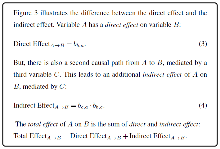
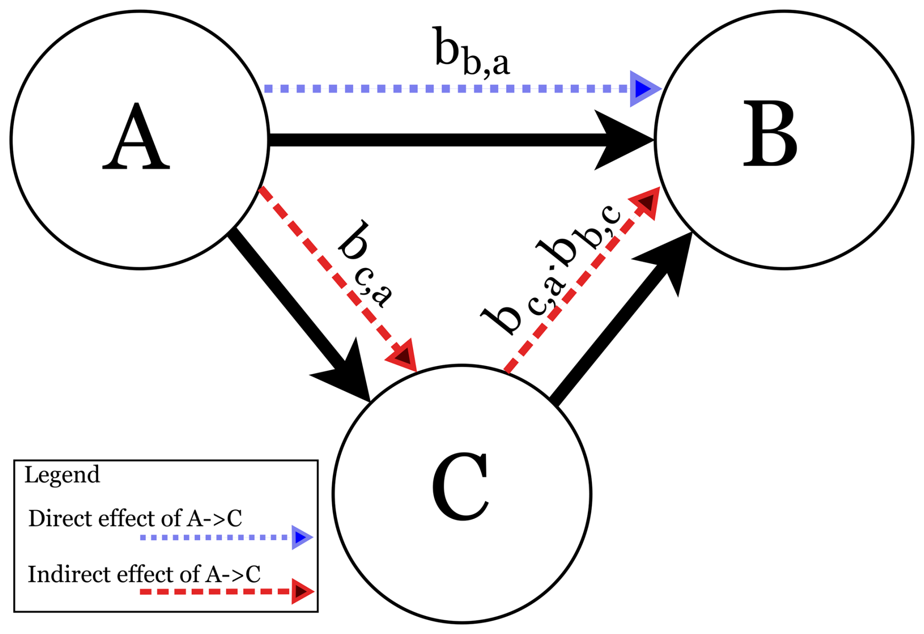
Causal models allow us to distinguish between a direct effect, which includes the part of the total effect of a forcing that acts immediately on an outcome, and the indirect effect, which accounts for the share of the effect size that is mediated through another factor. In other words, the distinction between direct and indirect effects is defined with respect to an a priori assumed causal graph. With such a graph, our frameworks estimates the magnitude of these effects conditional on the specified causal paths which usually cannot be identified from observational data alone.

Box 3 Definition of direct and indirect effect.

Earlier studies investigating the correlations between DGM concentration, solar radiation and temperature relied on discrete sampling campaigns with limited temporal resolution (Amyot et al., 1997; Gårdfeldt et al., 2001; Dill et al., 2006). However, solar radiation varies on a timescale of minutes, whereas sea surface temperature responds more slowly due to the thermal inertia of water. Low-frequency data collapse these distinct timescales which makes the variables statistically collinear and inseparable. Therefore, in order to separate the direct effect of solar radiation on mercury concentrations from the indirect effects mediated by sea surface temperature, the data must contain sufficient variability in both the exposure and the mediator. Also, since sea surface temperature already is used to calculate DGM (see Eqs. 1 and 2), C_MW was chosen as outcome variable instead of DGM in this study. This study provides data with high temporal resolution from automated long-term measurements of gaseous Hg concentration, solar radiation and surface seawater temperature. By using causal modelling, this study extends prior correlation-based research by quantifying the direct and indirect effect sizes of solar radiation on Hg concentration in seawater.

Box 4 Definition of direct and indirect effect.

The presence of additional factors can influence one or more predictor variables and the outcome at the same time can lead to confounding and bias in the estimated effect size between a predictor variable and the outcome. In our observational study, we considered wind, measured as wind speed W as potential confounding factors and the speed of the water pump, measured as r_W, as disturbing instrument-intrinsic factor. We expected wind to affect C_MW by diffusing mercury and to affect T_S through heat transfer and evaporation of water. Furthermore, we know that a fluctuating pump speed can influence the measured Hg concentration C_MW. We also assume that the pump speed can be influenced by solar radiation and temperature (e.g., through the growth of algae that clog the pump inlet) and by wind which causes waves that can affect the inlet of the pump. The identification of these confounding and disturbing factors led to the development of an additional model that was also tested in this study. This was done to identify how important they are to our measured C_MW and how they would affect the desired study of association between Sol and C_MW. Ultimately, this study aims to use causal and statistical modelling to infer the effect sizes of different forcings, such as solar radiation, sea surface temperature, wind speed, and water flow on C_MW.

Box 5 Definition of direct and indirect effect.

4.1.2 Step 2: Encode prior scientific knowledge and assumptions as a set of different plausible causal models in the form of DAGs

In this study, we intended to identify the effect of solar radiation Sol on the measured Hg concentration C_MW. Figure 4 provides an overview of three plausible models of the cause-effect relationships between the variables in this observational study, given the assumptions that Sol always affects T_S.

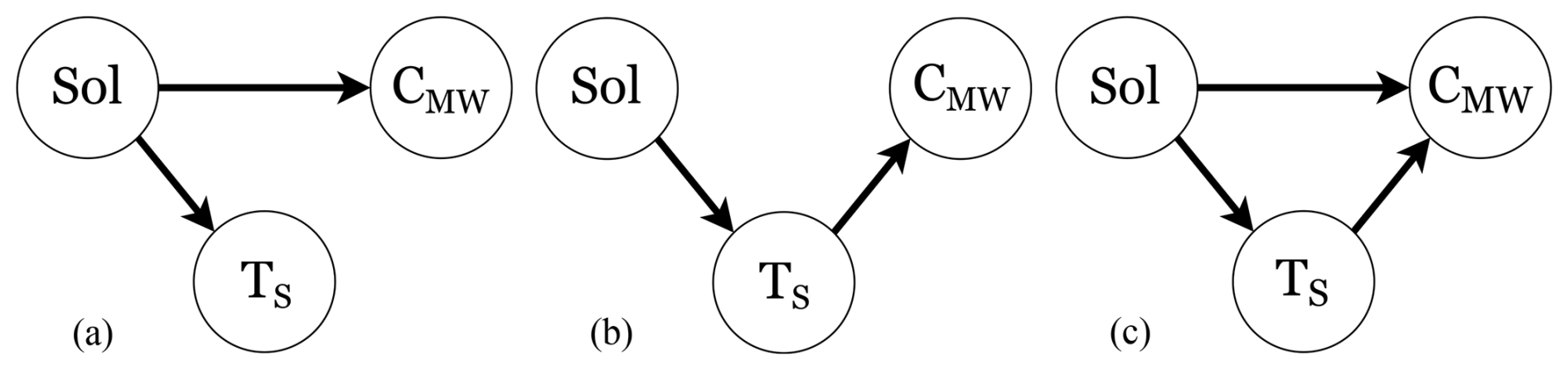
Figure 4 Directed Acyclic Graphs (DAGs), which encode assumptions about causal relationships between variables in the dataset.Sol: solar radiation; T_s: surface temperature of water; C_MW: Hg concentration. (a) Model m₁ representing an effect of Sol on C_MW and on T_S. (b) Model m₂ representing an effect of Sol on C_MW mediated by T_S. (c) Model m₃ representing an effect of Sol on T_s and C_MW and an effect of Sol on T_S.

The identification of the confounding factor wind speed W and the disturbing instrument-intrinsic factor water pump speed r_W resulted in the development of a fourth model, m₄, presented in Fig. 5.

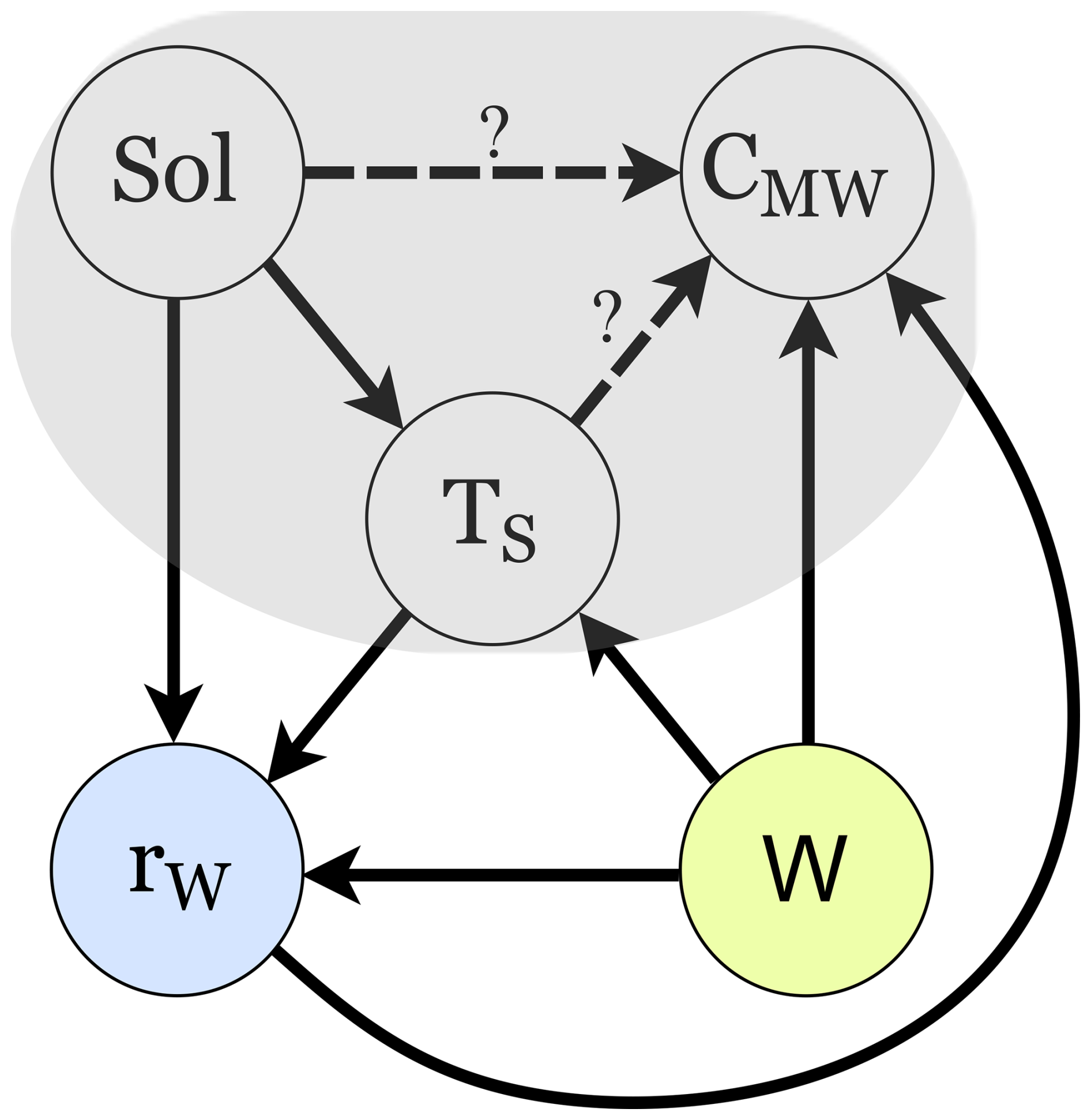
Figure 5 Model m₄ extending models m₁ − m₃ with external factors W representing wind and r_W representing water pump speed.

We first had to investigate which of the “base” models m₁ − m₃ is most plausible given the data. Then, we included the external factors in m₄ and estimated if the influence of the external factors is so strong that they could compromise our choice of “base” model³

4.1.3 Step 3: Derive independence criteria from the causal models

The DAGs shown in Fig. 4 provide information about plausible cause-and-effect relations and expected associations between the variables of interest. We expect an association between two variables if there is a cause-effect relationship between them⁴. However, association alone does not provide information about the direction of cause and effect. If we find an association between solar radiation (Sol) and surface temperature (T_S) in the data, we assume from experience that it is the sun radiation that causes the change in surface temperature. On the other hand, the absence of an arrow between two variables suggests that there should be no association in the data. In the DAG depicted in Fig. 4a, the solar radiation acts as common cause on the measured Hg concentration (C_MW) and the water surface temperature. Because of Sol acting as common cause, we will see a spurious correlation between C_MW and T_S in the data. This is called confounding and, in the DAG of Fig. 4a, Sol is therefore a confounding variable. Association can flow “anti-causally”, i.e., against the direction of cause-effect, from T_S to Sol and from there in the direction of cause to C_MW. Pearl et Mackenzie describe this as “association that flows in any direction along the edges” (Pearl and Mackenzie, 2018). However, the flow of association between C_MW and T_S can be blocked by conditioning on Sol. Then, given that we condition the data on Sol, T_S and C_MW become independent.

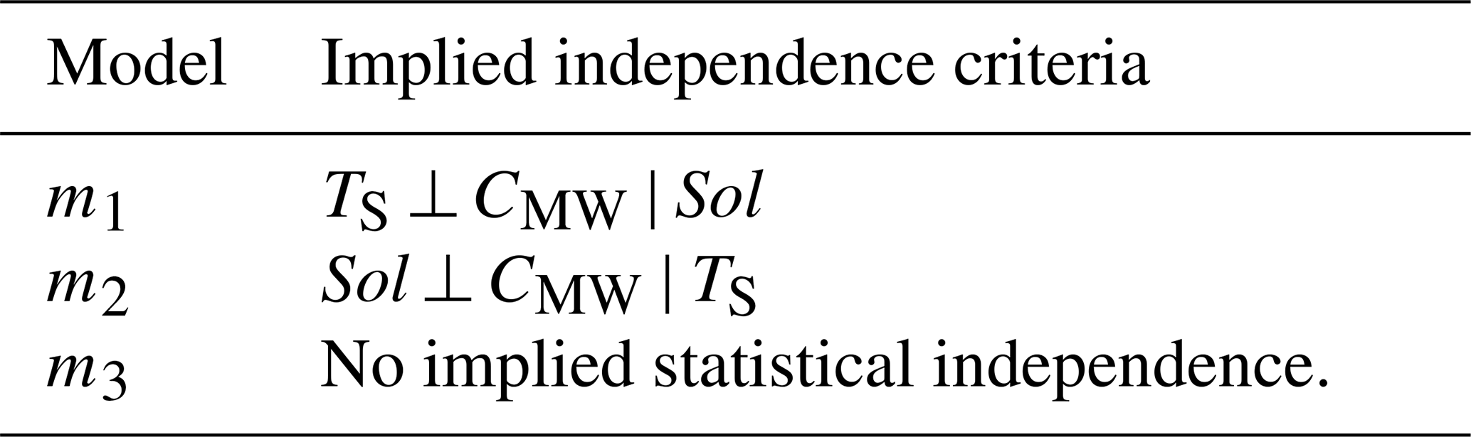
However, many researchers encounter the problem that a number of different causal models are possible given the correlations seen in the data. In our case, assuming that there is correlation between Sol, T_S, and C_MW, any of the cause models shown in Fig. 4 is plausible. There are two approaches that combined can help us identify the correct causal model: prior scientific knowledge and testing independence criteria. In fact, the causal models already include prior scientific knowledge by assuming the directions of cause and effect because there is no point in adding other compatible models in which the direction of cause and effect is obviously wrong, for example by assuming a change in T_S could causes a change in Sol. Each DAG in Fig. 4 suggests a set of conditional independence criteria for the research problem that can be used to validate or invalidate the assumptions about cause-effect relationships. Table 1 provides the implied independence criteria for the DAGs of Fig. 4. For our study, we used two approaches to test independence, namely visual inspection of scatterplots and regression analysis. We expected the coefficients of the independent variables to be close to zero if the independence assumption holds. Non-parametric measures of association, such as the Spearman's rank correlation coefficient are not well suited to testing conditional independence between three continuous variables because these measures typically assess association, not independence, between only two continuous variables.

Table 1 Implied statistical independence criteria based on assumed causal relationships in Fig. 4.

4.1.4 Step 4: Generate simulated data based on causal models and identified independence criteria

Simulated data were generated for each of the proposed causal models. Each simulated dataset was generated from a data-generating process using forward-sampling with fixed parameter values that reflect the causal assumptions encoded in the DAGs. As software, we used R with the rethinking package and Stan as underlying inference engine to implement the generative models. The simulations serve as a verification step to test if the statistical models can recover known parameters under assumed causal structure. They do not serve as a substitute for inference on observational data. Further details and results of the simulation are presented as supplementary material in Appendix B.

4.1.5 Step 5: Build statistical or machine-learning (ML) models for each alternative causal model

Statistical modelling

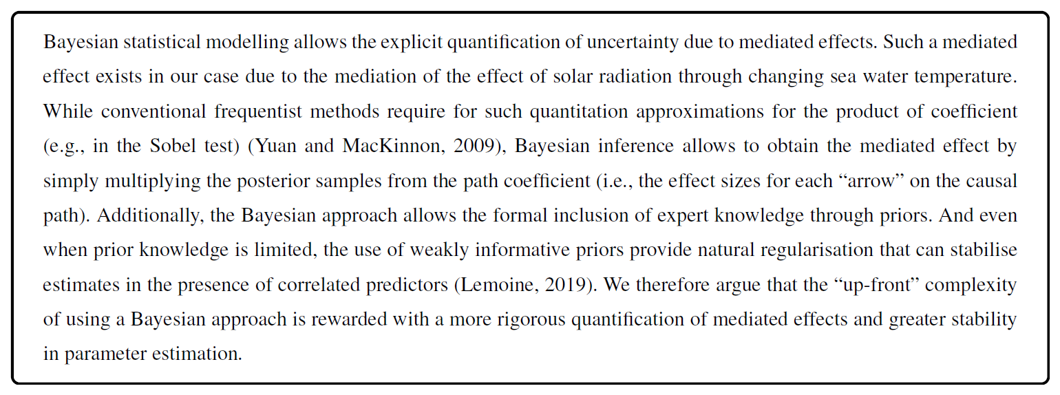
The aim of the statistical modelling for this research was to explore the causal relationships between the variables in the dataset. Initially, we built three Bayesian generalised linear regression models (GLMs) based on the causal models of Fig. 4. GLMs are a flexible family of statistical models widely used in empirical science (Furia et al., 2019; Gelman et al., 2020). They extend linear regression methods by introducing link functions and data type specific probability distributions which provides more flexible and accurate modelling of relations between variables in the dataset. We applied Bayesian data analysis (BDA), in combination with linear regression models, as a simple form of iterative ML. It is iterative in the sense that availability of new data in BDA allows for an update, not a complete recalculation, of the inference results.

Box 6 Justification for the Bayesian approach.

We followed a mathematical description of the statistical model which is standard in statistical journals and outlined in three steps in Chap. 4.2 of McElreath (2020):

• Data are represented as variables. Unobservable characteristics like averages, rates, etc. are defined as parameters. Each variable is either defined through other variables or probability distributions. Initial probability distributions assigned to the parameters are called priors.

• The combination of variables, parameters, and their probability distributions form a joint generative model which can be used to analyse relations between variables, estimate parameters, infer unobserved variables, and predict future observations.

• All predictor variables are standardised to avoid numerical problems due to large values and to allow for negative values (Marquardt, 1980). Standardisation means that all values are centred on zero and that the data have a standard deviation of one. This approach is also known as z-score normalisation.

After we identified model m₃ as most appropriate (see Sect. 5.2), we extended it to model m4, shown in Fig. 5, by introducing the external confounding element wind W and the instrument-intrinsic factor pump speed r_W.

The mathematical definition of the models are listed in Table 2.

Table 2 Model specifications.

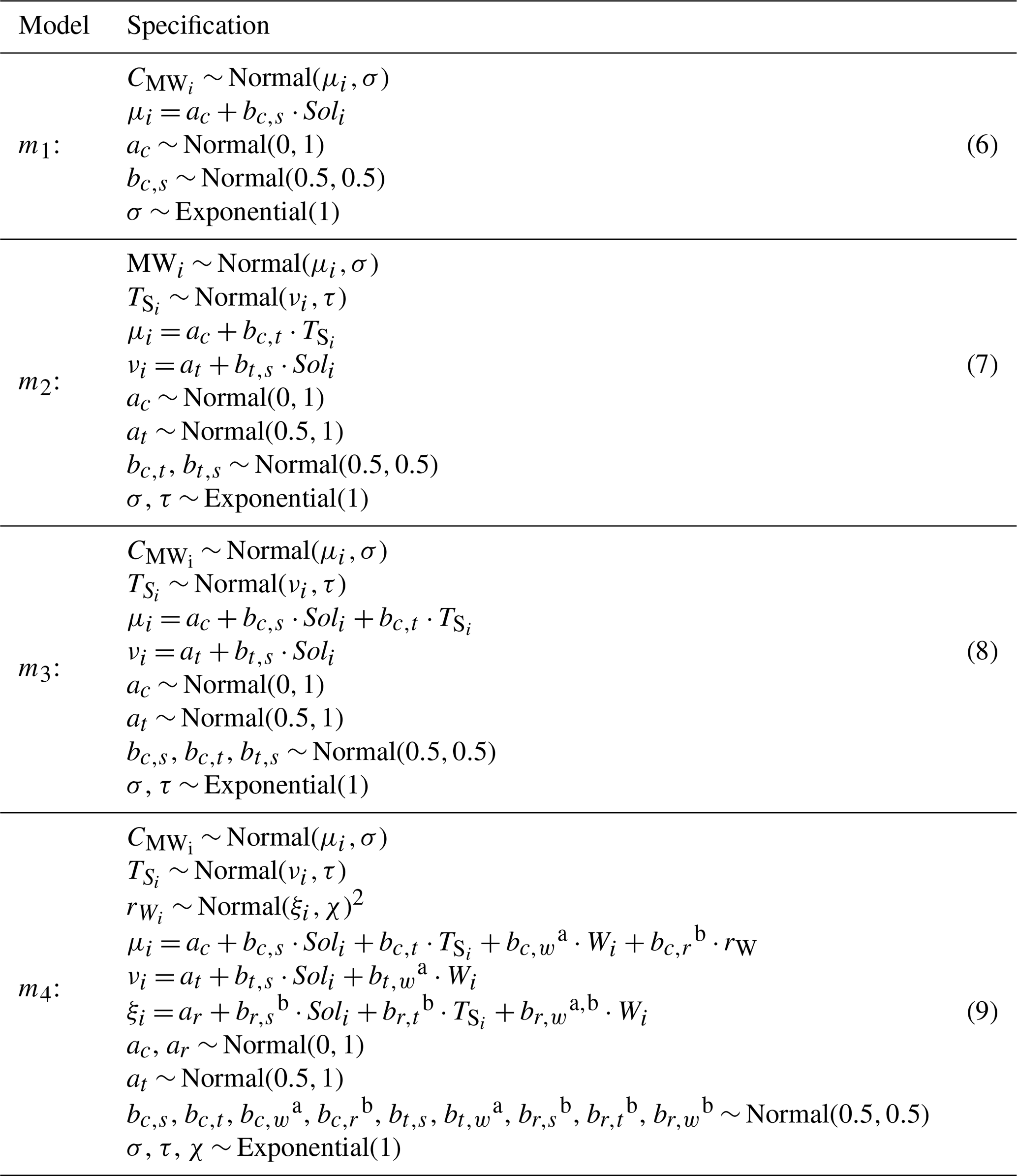
^a Terms that relate to the wind speed W. ^b Terms that were relate to the speed-pump r_w.

The four resulting statistical models for predicting C_MW differ due to different assumptions about cause-effect relationships as shown in Figs. 4 and 5. However, the models share a common structure: they contain definitions of the likelihood that define probability distributions of the outcome (in our case the measured C_MW) given a set of parameters that define this probability distribution, for example through the mean μ and standard deviation σ for Normal distributions. Models m₂ and m₃ contain two likelihoods because in both models Sol affects the surface temperature T_s which then affects the measured C_MW. Therefore, we needed to define two linked regression models, one for T_s with Sol as the predictor variable, and one for C_MW with T_s as the predictor variable for model m₂, and both Sol and T_s as the predictor variables for model m₃. The parameters of the likelihood are declared in the form of either a deterministic function assignment (denoted through =) or stochastic relations (denoted through ∼), i.e., a mapping of a variable or parameter onto a distribution. When a parameter (e.g., b_(c,t)) is mapped onto a distribution (e.g., the Normal distribution), this distribution is then referred to as a prior distribution.

Variables

There are four main variables in models: $C_{{\mathrm{MW}}_i}$ represents the measured Hg concentration, associated via Eq. (2) to DGM. It is chosen as outcome variable for all models. The index i denotes an individual data frame in the total dataset. $T_{{\mathrm{S}}_i}$ represents the surface temperature of the water and is a predictor variable in models m₂ − m₃. Sol_i is another predictor variable in all models and represents solar radiation. In models m₂ and m₃, Sol_i is also a predictor for $T_{{\mathrm{S}}_i}$. The additional model m₄ includes the confounding variable W and instrument-intrinsic factor r_W. The biasing influence of these variables on our effect size estimates can be compensated for by including them in the prediction model for $C_{{\mathrm{MW}}_i}$ and $T_{S_i}$. In this way, we “block” any anti-causal flow of association between T_S and C_MW via W and r_W. The model m₄ including the external influences also includes parameters describing the effect size of these external influencing factors W and r_w: b_c,w and b_c,r represents the effect size between C_MW and W, respectively r_W, b_t,w and b_c,t between T_S and W, respectively r_W, b_r,s between Sol and r_W, and b_r,w between W and r_W. The parameter ξ represents the estimated standard variation for the r_W data.

Likelihood

The role of the likelihood is to link the observed data to the distributions of the inferred model parameters (Furia et al., 2019). The likelihood provides a distribution function of how well the model explains the observed data given an inferred set of distributions for the model parameters. We assumed that the observed data can be represented through a Normal distribution because the central limit theorem states that the distribution of the sum of a large number of independent processes approaches a Normal distribution and environmental phenomena typically involve the aggregation of a large number of underlying processes. Furthermore, we had no reason to assume another distribution for the outcome C_MW. However, Appendix G discusses the alternative choice of a log-normal likelihood for C_MW that can often be appropriate for environmental data. As part of the GLM, the likelihood distribution is further specified through a linear model, i.e., the mean (e.g., μ is constructed through a linear combination of other parameters (e.g., a_c + b_c,s) and predictor variables (e.g., Sol_i). This link function between the likelihood and the parameter distribution of the model can take any functional relation based on the prior knowledge of the researcher. We decided to use a linear model because we do not have any prior knowledge that would justify the use of any other functional form, and it represents the most conventional functional relation between an outcome and its predictor variables. Bayes’ rule is then used to iteratively calculate a posterior distribution for the parameters of the model given the prior distributions, the observed data, and considering the likelihood, i.e., how well the currently assumed parameters explain the data:

$$\begin{array}{}\text{(10)}& \text{posterior}\propto \text{prior}\cdot \text{likelihood}\end{array}$$

Priors

In general, a prior tells researchers what assumptions are made about a parameter before they see any observed data. These assumptions can range from highly informative, where the distribution encodes strong prior beliefs about the parameter values, through weakly informative priors that provide mild regularisation, to non-informative priors that have very little influence on the posterior distribution. It is important to note that priors are continuously updated with the available observed data. With each iteration in BDA, the posterior will be used as new prior for the next iteration. That means, that the more data is available, the less influence prior beliefs have. With each iterative update, the prior distribution will be more influenced by the data distribution and therefore become increasingly dominated by the likelihood. In BDA, weakly informative priors are preferred in applied regression modelling because they provide mild regularisation (Lemoine, 2019). This prevents, for example, extreme parameter values, while at the same time allowing the data to shape the posterior distribution.

For the models of this study, we used weakly informative priors for all parameters. Because all predictor variables were standardised, such that the coefficients represent effects on a common scale, we used Normal priors with modest location and scale parameters that encode a coarse, “order-of-magnitude” expectation about plausible effect sizes and allowing both positive and negative effect sizes. Furthermore, the Normal distribution can represent a wide range of shapes from perfectly symmetric to slightly skewed which makes it a suitable choice if no other strong information is available about the shape of the prior distribution. We assumed exponential distributions for the parameters related to the variances because these must always be positive. The plausibility of the priors was assessed using prior predictive simulations for our models m₁ to m₄, which are presented as supplementary material in Appendix C.

4.1.6 Step 6: Verify the models on the simulated data

In this step we show that the models can estimate the parameters set for the simulation and identify independence relations in simulated data. Each model was verified on the simulated data sets created in Step 4 by comparing the posterior parameter estimates with the known parameter values used in the data-generating process. The verification was considered successful if the posterior means recovered the true parameter values and if parameters corresponding to absent causal paths were estimated close to zero. The results of the parameter estimates for all models under simulated data are given in Appendix B.

4.1.7 Step 7: Run the models on observational data

Inferring data from the models means predicting the distributions of the parameters as well as predicting the posterior distributions of the outcome (i.e., C_MW in all models) given the observed data for T_S, Sol, C_MW, and in case of model m₄ the external influences W and r_W. We applied a stochastic process known as Markov Chain Monte Carlo (MCMC) to find the posterior distribution. MCMC is considered a standard approach for Bayesian Data Analysis and an introduction to the technique is available in Brooks et al. (2011). In brief, MCMC works by running a Markov chain that samples data from posterior distribution. In a Markov chain, the next state only depends on the current state and not on any other states before that. Different techniques, such as Hamiltonian Monte Carlo (HMC), can be applied to find the next state in the Markov chain. In HMC, the next state is not determined purely at random, but instead through the gradient of the posterior distribution which allows an adaptive step size for each new state. To find the posterior distributions for the parameter and outcome using MCMC with HMC, we used the R-packages rethinking (McElreath, 2023) and Rstan (Stan Development Team, 2024).

4.1.8 Step 8: Checking of independence criteria and parameter estimates

Initially, scatter plots were created to check for statistical independence between the variables. These are presented and discussed as supplementary material in the Appendix E. Furthermore, the parameter estimates can be used to identify statistical independence between variables, which is discussed as part of the results in Sect. 5.2. The results of the independence check were compared with the established independence criteria to provide evidence for a final candidate model.

4.1.9 Step 9: Validating the plausibility, workability, and adequacy of the models

Furia et al. (2022) recommend validating three characteristics of statistical models for BDA: The models must be plausible, workable, and adequate.

Plausibility

Plausibility can be achieved by checking that the model is “consistent with (expert) knowledge about the data domain” (Furia et al., 2022). The key aspect here is that the models should include reasonable priors that they are consistent with expert knowledge and that are neither too permissive nor too constraining, especially in the case of limited available data (McElreath, 2020). The plausibility of the priors can be checked using prior predictive simulations which we provide as supplementary material in Appendix C.

Workability

Second, the models must be workable, i.e., it must be computationally possible to fit the models to the provided data without, for example, encountering numerical difficulties. Numerical difficulties can arise from multicollinearity (Furia et al., 2022): if two variables in the data are very strongly correlated, the model cannot determine the ratio of contribution to the outcome between the two variables and we cannot determine the effect size for each of the variables. To check the workability of a model, the sampling process can be independently repeated a few times and the similarity between each sampling process can be estimated through the ratio of within-to-between chain variance $\widehat{R}$. An $\widehat{R}$-value close to 1 indicates a stationary posterior distribution which is desirable. Another metric that provides an indication of the workability of the model is the effective sample size. It indicates the size of samples that are not autocorrelated, i.e., it measures how much information is lost due to information redundancy between samples. A recommendation is that the effective sample size should be at least 10 % for each estimated parameter (Furia et al., 2022). Other indicators of numerical problems are divergent transition warnings that statistical toolboxes such as rethinking or the underlying Stan library may raise when evaluating the posterior distributions of the models. As part of the model validation for the proposed models we provide the $\widehat{R}$-values and effective sample sizes for each model together with the detailed inference results in Appendix F. We also checked for warnings of divergent transitions while training the models on the data. A detailed discussion of the convergence assessment, including visual trace plots for the effect size parameters, can be found in Appendix H.

Adequacy

A final aspect of model validation is that the models must be adequate for the problem under investigation. An adequate model can generate data that are similar to the observational data (Furia et al., 2022). Adequacy can be tested by comparing the posterior predictive plots with the empirical data. A posterior predictive plot visualises the posterior predictive distribution which is obtained by evaluating the posterior distributions of the likelihood parameters, in our case μ and σ, and then sampling from the resulting probability distribution. We provide posterior predictive plots for each model as part of the model evaluation in Fig. 11. Statistical models can also be compared to each other using information criteria. The Watanabe-Akaike Information Criterion (WAIC) is an example of an information criterion commonly used for relative comparison of statistical models (Watanabe and Opper, 2010). It approximates the relative out-of-sample Kullback-Leibler (KL) divergence, i.e., it tells us something about the relative “statistical distance” of a model from the data. Because information criteria rely in some way on the KL divergence, which is not a metric but a relative measure, WAIC, and most other information criteria, are also relative measures of the adequacy of the models. They do not provide an absolute metric that can be used to determine the absolute adequacy of an individual model. Instead, information criteria such as WAIC can be used to compare models against each other. We provide WAIC scores for all models as part of the model evaluation in Sect. 5.3 and in Fig. 12. Wheras WAIC provides an expected out-of-sample predictive accuracy estimate, the coefficient of determination R² summarises in-sample explanatory fits. In this analysis, WAIC and R² are consistent for the models, but if they were to diverge, it would indicate that a model either fits the observed data well but generalises poorly, or generalises well but shows a reduced in-sample fit.

4.1.10 Step 10: Report and interpret the results

The results, discussions and answers to research questions are presented in Sects. 5 and 6.

5 Results

5.1 Measured data

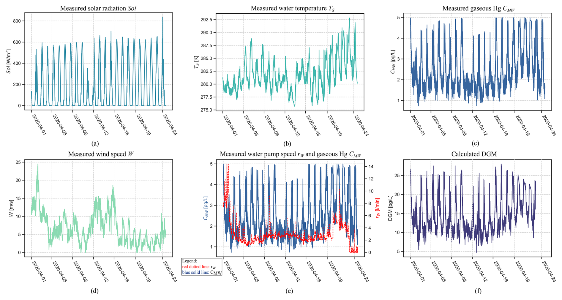
The data used for this study were collected between 1 April 2020 (13:20 UTC+1) and April 25th 2020 (02:29 UTC+1). Figure 6 and Table 3 summarise and present the observed data. The data have a coverage rate of 92 % for all measured parameters with 6149 valid data points. The month of April was chosen due to the good data coverage, which makes it already visually possible to see some co-variations between the variables in the data.

Table 3 Summary statistics of calculated DGM and the measured parameters C_MW, solar radiation (Sol), surface water temperature (T_S), windspeed (W), and speed of the water pump (r_W) during April 2020.

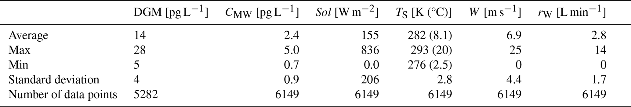
The measured C_MW in Fig. 6c show clear diurnal patterns with peaking concentrations during daytime and lower concentrations during night-time. This coincides with the measured solar radiation shown in Fig. 6a. Solar radiation shows clear diurnal patterns with higher values during the day and lower values during the night, as to be expected. It is even possible to see in the patterns of the data that 11 April was a cloudy day, as less radiation was measured at noon. This explains why the peak in measured C_MW was lower at this time. The measured surface water temperature, plotted in Fig. 6b, also shows variations with higher temperatures during the day and lower temperatures during the night, suggesting an association between solar radiation and surface water temperature. In Fig. 6d we also plotted C_MW to show the distinct covariation of the pump speed r_W and the measured Hg concentration C_MW. Calculated DGM, shown in Fig. 6f, show similar diurnal patterns as for C_MW. The average concentration during the measurement period was 14 pg L⁻¹ (Table 3). During the summers in 1997 and 1998, Gårdfeldt et al. (2001) measured DGM by manual sampling at 20 cm depth in open seawater, about 1 km from the Kristineberg Marine Research Station, resulting in DGM concentrations varying between 40 and 100 pg L⁻¹. However, it differs about 20 years between their and our measurements. More recent continuous measurements of DGM, performed in spring 2015 at the Råö/Rörvik station in Sweden (about 160 km south of Kristineberg), showed an average DGM surface concentration of 13 pg L⁻¹ (Mastromonaco, 2016), which is in good agreement with our study. The literature review presented in Mastromonaco et al. (2017) show surface DGM concentrations varying between 11 and 32 pg L⁻¹ in the Baltic Sea (15–20 pg L⁻¹ in spring), 11–52 pg L⁻¹ in the North Sea, 12 pg L⁻¹ in the North Atlantic Ocean (summer) and about 20–30 pg L⁻¹ in the Mediterranean Sea.

Figure 6 Observational data collected in April 2020 used in the analysis.

5.2 Parameter estimates and causal inference

After fitting the models to the observed data, we obtained posterior distributions for each parameter of the models. Figure 7 shows the estimates for the constant parameters a_C and a_T of the models listed in Table 2. The first parameter a_C is the constant offset in the Sol → C_MW ← T_S part of the models. It is approximately equal to the mean of the C_MW values in data which is 2.4 pg L⁻¹. The estimate for a_T is close to zero for all models because we have standardised the predictor parameters Sol and T_S. Figure 8 provides the estimates for the coefficients of effect sizes b_t,s, b_c,s, and b_c,t. These estimates are important to answer what the direct and indirect effect of solar radiation on Hg concentration are (RQ1).

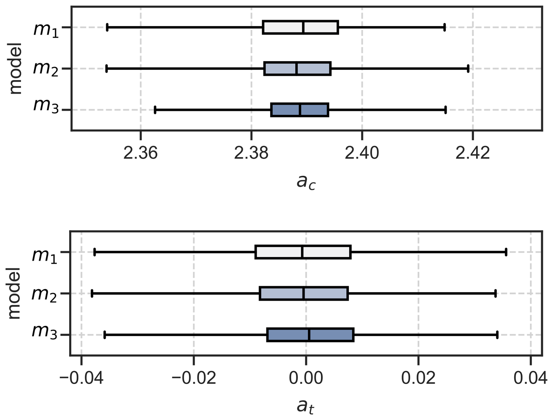
Figure 7 Coefficient estimates for a_c, the constant term for C_MW, and a_T, the constant term for T_S.

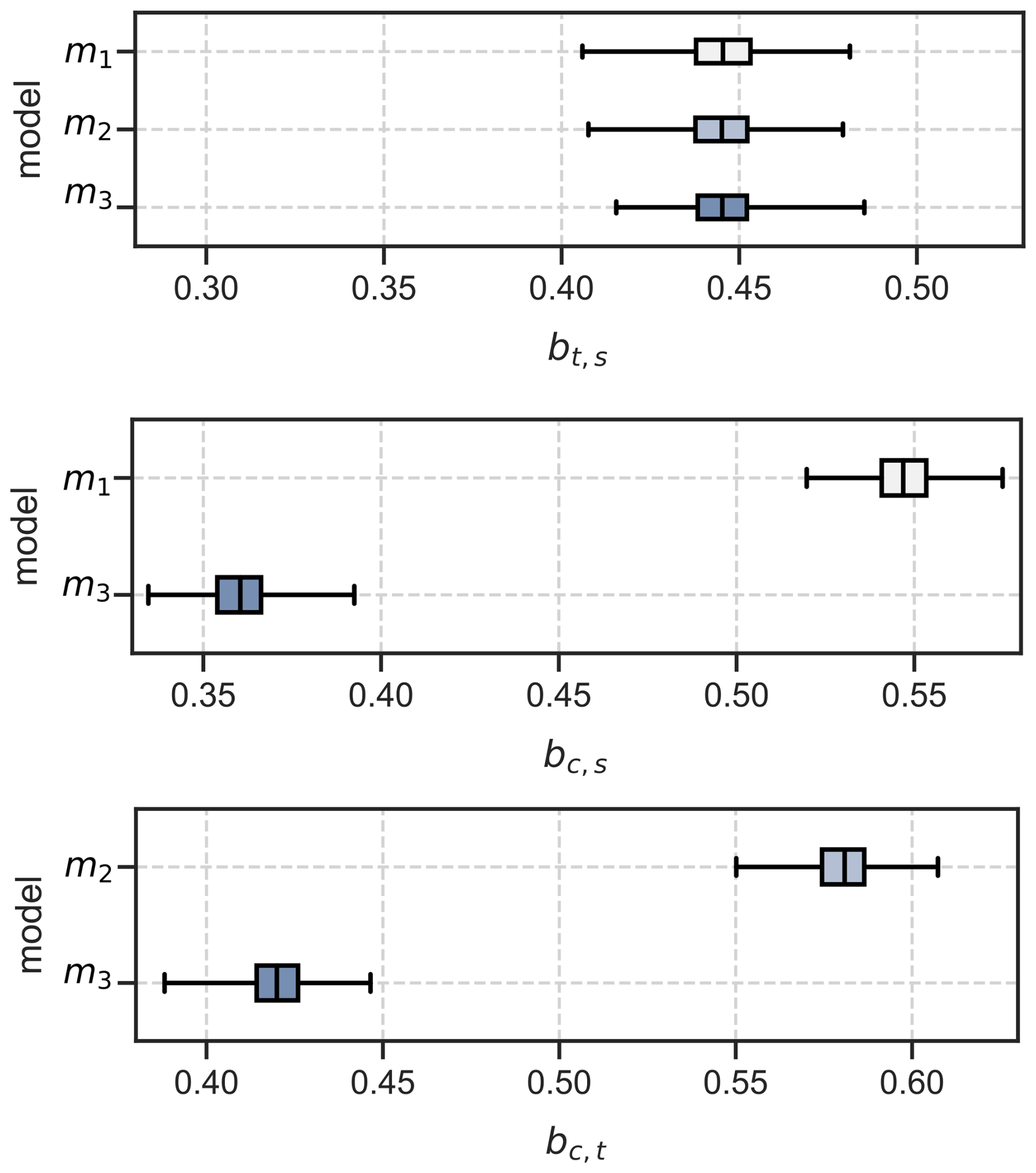
Figure 8 Coefficient estimates for the effect size of solar radiation on temperature (b_t,s), the effect size of solar radiation on Hg concentration (b_c,s), and the effect size of sea surface temperature on Hg concentration (b_c,t).

None of the effect size estimates are zero, which means that we cannot assume any statistical independence between the variables. We confirmed these results using manual examination of scatter plots, which is outlined as supplementary material in Appendix E. Hereafter, we propose model m₃ is the most plausible causal model for the variables of interest.

5.2.1 Detailed argumentation on why model m₃ is most plausible

The parameter b_c,s is the effect size between the standardised predictor variable Sol and C_MW. It gives us an estimate of the strength of the association, and hence the assumed causal relationship, between solar radiation and measured Hg C_MW. The estimated mean value for b_c,s is 0.547 for model m₁ and 0.360 for model m₃. Model m₂ has no estimate for b_c,s because it assumed (incorrectly) a-priori that there is no causal relationship between Sol and C_MW. Because we used standardised predictor variables, these effect size estimates imply that 1 standard deviation of solar radiation is associated with a change in C_MW of 0.547 pg L⁻¹ and, respectively for model m₃, 0.360 pg L⁻¹. Dividing the estimated effect size b_c,s by the original standard deviation of the data for Sol gives the de-standardised effect size estimate $b_{c,s}^{\mathrm{o}}$:

$$\begin{array}{}\text{(11)}& b_{c,s}^{\mathrm{o}}o={\displaystyle \frac{b_{c,s}}{{\mathit{\sigma }}_{Sol}}}.\end{array}$$

Using the standard deviation of Sol given in Table 3, model m₁ estimates that an increase of solar radiation by 1 W m⁻² is associated with an average increase in C_MW of $\frac{\mathrm{0.547}}{\mathrm{206.29}}$ pg L⁻¹(W m⁻²)⁻¹ = 0.00265 pg L⁻¹(W m⁻²)⁻¹ Model m₃ estimates an increase in C_MW of $\frac{\mathrm{0.360}}{\mathrm{206.29}}$ pg L⁻¹(W m⁻²)⁻¹ = 0.00175 pg L⁻¹(W m⁻²)⁻¹, which is 66 % of the estimate from m₁. Assuming that there is a causal relationship between solar radiation and C_MW, which model gives the correct estimate of the strength of the causal relationship between Sol and C_MW?

5.2.2 Total effect and direct effect

In fact, both estimates of the strength of the causal relationship are correct. However, model m₁ provides with b_c,s the total effect. Model m₃ provides instead the direct effect of Sol on C_MW. If there is a causal relationship between Sol on C_MW, there is also a “flow” of association between these variables. This “flow” of association can take different “routes” between the variables. In our case, solar radiation Sol has a direct effect on the concentrations of Hg (C_MW), which means that we can measure an association between these two variables. Its effect size is estimated in our models as b_c,s:

$$\begin{array}{}\text{(12)}& {\text{Direct Effect}}_{Sol\to C_{\mathrm{MW}}}=b_{c,s}.\end{array}$$

However, Sol also affects the sea surface temperature T_S, which in turn affects C_MW. Besides a direct effect, Sol also has an indirect effect on C_MW, mediated by T_S. The indirect effect of Sol on C_MW can be calculated by multiplying the effect sizes for the paths Sol → T_S and T_S → C_MW:

$$\begin{array}{}\text{(13)}& {\text{Indirect Effect}}_{Sol\to C_{\mathrm{MW}}}=b_{t,s}\cdot b_{c,t}.\end{array}$$

In summary, a part of the association between Sol and C_MW “flows” via T_S. The total effect of Sol on C_MW is the sum of direct effect and indirect effect. This definition holds regardless of the sign of the individual path-specific effects: indirect effects with opposite signs represent competing causal mechanisms that (partially) can cancel each other out.

$$\begin{array}{}\text{(14)}& {\text{Total Effect}}_{Sol\to C_{\mathrm{MW}}}=b_{c,s}+b_{t,s}\cdot b_{c,t}.\end{array}$$

For model m₃, the direct effect equals, on average, to b_c,s = 0.360 and the indirect effect equals, on average, to $b_{t,s}\cdot b_{c,t}$ = 0.445 ⋅ 0.420 = 0.187, as illustrated in Fig. 9b. Using Eq. (14), the total effect of Sol on C_MW is then 0.360 + 0.187 = 0.547, which is exactly the estimate for b_c,s that model m₁ provided. By removing the path between T_S and C_MW, we do not allow a “flow” of association between T_S and C_MW in model m₁, as illustrated in Fig. 9a. The association related to the indirect effect of Sol on C_MW that is mediated by T_S, therefore cannot flow through T_S and is instead “rerouted” onto the direct path between Sol and C_MW (red, wide dotted line in Fig. 9a). Consequently, the effect size b_c,s, estimated by model m₁, is the sum of the direct and indirect effects, thus in fact the total effect of Sol on C_MW. Although individual mechanisms, such as the temperature dependence of Henry's law, may suggest opposing effects on equilibrium DGM, the causal model in this study is specified for measured mercury concentrations C_MW. Empirically, the inferred effect b_c,t of seawater temperature T_S on C_MW is positive in the observational data, which suggest that temperature-related processes in this measurement context are stronger than the opposing sub-mechanisms.

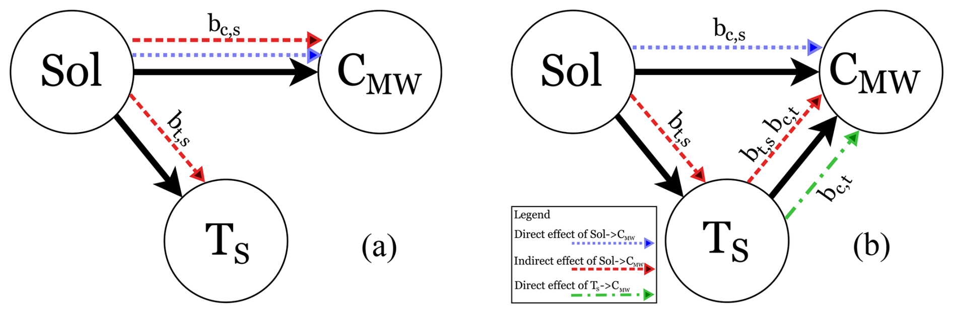
Figure 9 DAGs with illustration of flow of association. Red, wide dotted line: association of solar radiation Sol on Hg concentration C_MW, mediated by sea surface temperature T_S. Blue, dense dotted line: association of Sol on C_MW, not influenced by Sol. Green, mixed dotted line: association of T_S on C_MW. (a) Model m₁ where the path T_S → C_MW is not allowed and the indirect effect of Sol on C_MW is therefore “rerouted” on top of the direct effect of Sol on C_MW. (b) Model m₃ where the path T_S → C_MW is allowed and the indirect effect of Sol on C_MW therefore can flow via T_S.

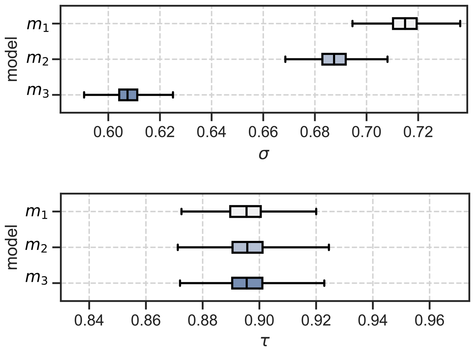
A similar line of argumentation can be provided for the difference of the estimate of b_c,t between model m₂ and model m₃. Because the path Sol → C_MW is not allowed in model m₂, the association related to the direct effect of Sol on C_MW is “rerouted” on the path Sol → T_S → C_MW. This results in an overestimate of the direct effect b_c,t of T_S on C_MW. Due to the misspecification of models m₁ and m₂, these two models result in a higher standard deviation σ for the C_MW data as shown in Fig. 10 because the models cannot correctly map all association between Sol, T_S, and C_MW. However, the standard deviation τ for the relation Sol → T_S is identical for all models, because the path between Sol and T_S exists in all models. Table 4 summarises the estimated effect sizes for model m₃.

Figure 10 Estimates of standard deviation σ for C_MW and standard deviation τ for T_S.

5.2.3 Adding estimates for the effect of external influencing factors in model m₄

After having identified the most plausible “core” model, we extended it by adding estimates of external influencing factors. Wind, denoted as W, is an environmental factor that could affect the measurements of C_MW. The speed of the water pump, r_W, however, is a instrument-intrinsic factor that could have effect on the measurements for C_MW. In line with other predictor variables, we chose identical priors for W and r_W based on a prior predictive check. The results of the estimated effected sizes on C_MW of the updated model m₄ are presented in Table 4, while all parameter estimates are listed in Appendix F. The average effect size of wind W on surface temperature T_S, denoted as b_t,w is −0.24. This agrees with our expectations that an increase in wind speed results in a lowering of the sea surface temperature. The estimated average effect size of W on Hg concentration C_MW, denoted as b_c,w is −0.13. The estimated average effect size of wind is smaller compared to⁵ the effect sizes of surface temperature b_c,t = 0.43 and solar radiation b_c,s = 0.38. As we expected after inspecting Fig. 6e, the water pump speed r_W has a distinct effect on the measured Hg concentration C_MW, with an estimated average effect size of b_c,r = 0.27. An interesting observation can be made when estimating the effect sizes of the other environmental variables, Sol, T_S, and W, on the water pump speed. The effect sizes of solar radiation and sea surface temperature on the water pump speed are small with average effect sizes of b_r,s = − 0.04 and b_r,t = − 0.09 respectively. But the influence of wind speed on the water pump speed is strong with an average effect size of b_r,w = 0.27. All inferred effect sizes are listed in Table F1 in Appendix F. A possible explanation for the strong relationship between wind speed and water pump speed is that due to high winds, sea waves could have cleared the inlet of the pump from algae, resulting in a higher flow speed. Unlike model m₃, where the indirect effect of solar radiation on C_MW is only mediated by the sea surface temperature T_S, model m₄ allows for two additional mediation paths: Sol → r_W → C_MW, and Sol → T_S → r_W → C_MW. However, the latter mediation path contributes only very weakly to the total indirect effect due to the small effect of surface temperature on pump speed (b_r,t). In contrast to the effect of solar radiation on pump speed (b_r,s), which is also relatively small, the credibility interval of the effect size b_r,t, listed in Table F1, contains zero. We therefore cannot exclude the possibility that the effect of sea surface temperature on pump speed is practically negligible and consequently do not interpret this compound path as a substantively important part of the total indirect effect. In summary, the inclusion of the confounding external factor wind W and instrument-intrinsic factor water pump speed r_W lead to a noticeable increase in the estimated effect size of solar radiation Sol on measured Hg concentration C_MW by 6.3 % compared to the estimate of model m₃.

Table 4 Estimates of the direct, indirect, and total effects based on observed data in April 2020 without (model m₃) and with (model m₄) recognition of wind and pump speed as external influences. Bold values are mean values; standard deviations are in parentheses; 90 % confidence intervals are depicted in square brackets.

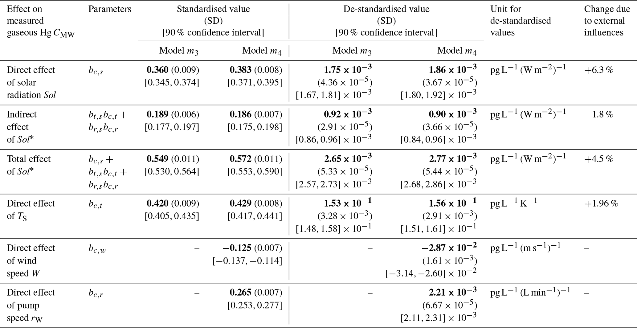
^* The additional compound mediation path Sol → T_S → r_W → C_MW ($b_{t,s}{b}_{r,t}{b}_{c,r}$) is practically negligible due to the small effect b_r,t which includes zero in its 90 % credibility interval (see Table F1).

5.3 Results from model validation on observed data

We have already established that model m₃ and its extension with external influences to model m₄ are most plausible. Furthermore, all models are workable meaning that it is computationally possible to fit the models to the data provided. Evidence for this claim is that the R² values for all parameters in all models are close to 1 indicating stable posterior distributions as listed in Table F1 in Appendix F. Further evidence of the workability of the models are the effective sample sizes n_eff which indicate that the samples contain sufficient information to infer the model parameters. The overall sample size was n = 6149. The smallest effective sample size occurred for parameter b_r,t of model m₄ with n_eff = 811 which is more than the recommended ratio of at least 10 % of the total sample size. We did not receive any numerical warnings during the training of the models. Finally, we also checked that the models are adequate by comparing the posterior predictive plots with the empirical data as shown in Fig. 11a–d. The closer the points in these plots are to the black diagonal line, the better a model can predict the outcome variable. It is obvious that model m₃ and m₄ seem most adequate to predict C_MW. This is further confirmed by plotting the posterior distribution densities, as shown in Fig. 11e. The posterior density of C_MW in this plot is closest to the observed data density for model m₄. We have also calculated the R²-values, shown in Fig. 11f), using the mean of the posterior predictions for C_MW for all models. Model m₃ has an R² value of 0.544 and model m₄ has the highest R² value of all models with a value of 0.626, which indicates a moderate to good fit to the data. It is important to remember that model m₃ only accounts for solar radiation, temperature changes and the interaction between these two external variables, and model m₄ adds the additional influences of wind and variation of the water speed pump. The models ignore any additional external factors that might influence C_MW. It is therefore a rather simple model of C_MW, but yet the fit to the data is quite acceptable.

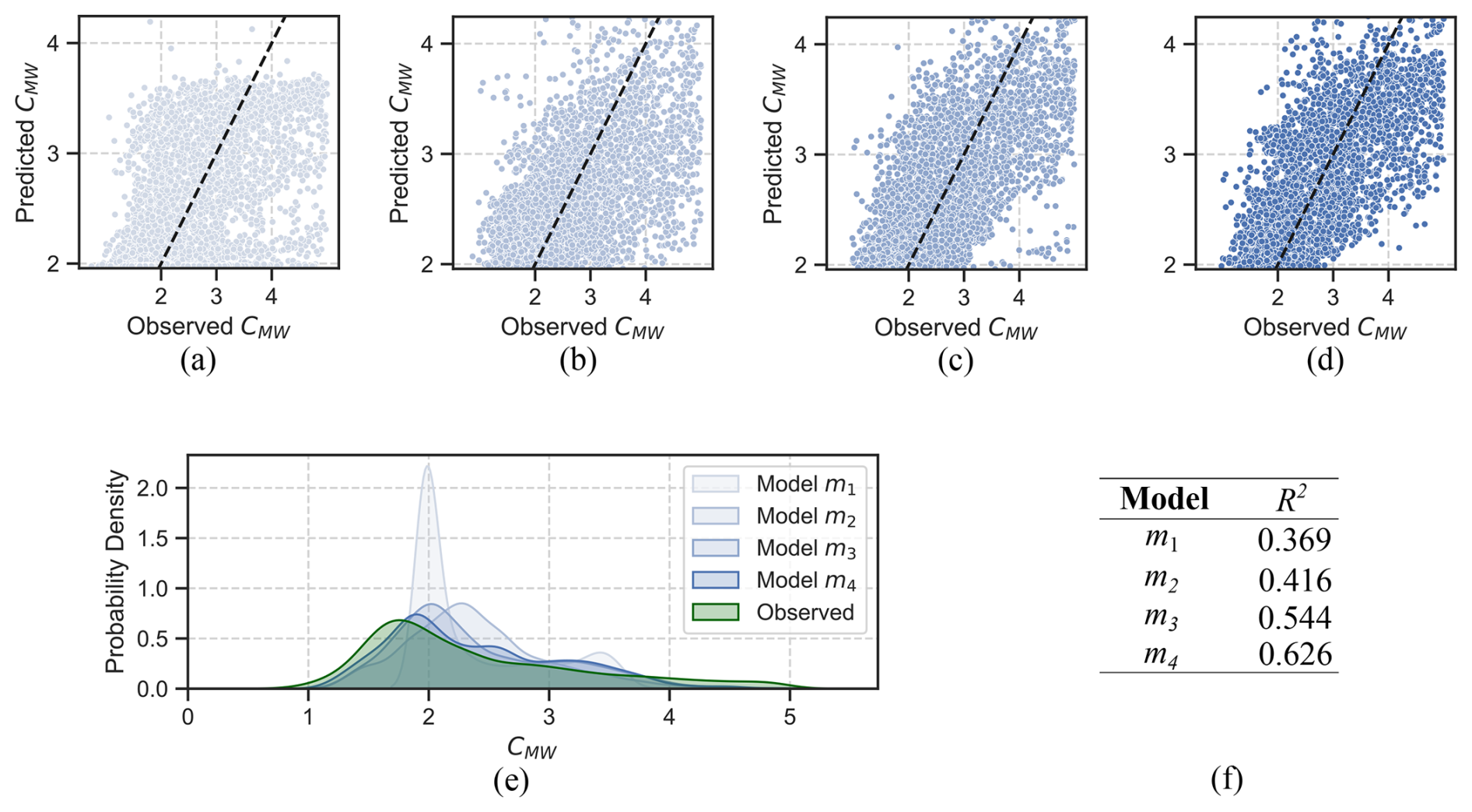
Figure 11 Posterior predictive plot for models (a) m₁, (b) m₂, (c) m₃, and (d) m₄. The dotted lines indicate where the posterior prediction and the sample match exactly. Panel (e) provides the posterior distribution density for all models. Panel (f) provides the coefficients of determination (R² values) for all models.

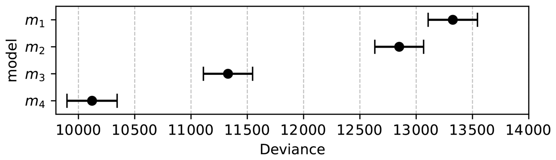
Finally, we calculated the WAIC information criterion which allows us to make a relative comparison of the statistical models. Figure 12 suggests that model m₄ has the lowest deviance and is therefore the most adequate model. A lower deviance calculated by WAIC indicates a smaller statistical distance between the estimated posterior distribution of the model and the probability distribution of the observed data which we have also checked manually using the posterior distribution density plots in Fig. 11e.

Figure 12 Comparison of models using WAIC.

6 Discussion

When using statistical or ML methods to analyse observational data, researchers need to distinguish between predictive and analytical models. In a predictive model, the aim is to use the data to train a model that predicts future trends in an outcome of interest. Any observed variable that adds predictive power reduces the uncertainty of the outcome, and these variables are typically strongly associated with the outcome of interest. ML algorithms therefore require large amounts of data to find as many associations in the data as possible. However, purely predictive models are black boxes in terms of which features, or variables, in the data contribute to the outcome and to what extent. A warning example of how adding any variable that adds predictive power can lead to erroneous conclusions on effect sizes is given in Appendix D.

Besides predicting future trends, environmental research also seeks understanding of why an outcome occurs and to quantify the effects that determine them. Therefore, researchers need to move away from purely predictive models, which work only with associations in the data. Instead, they should refocus on analytical models, which provide estimates of the strength of different cause–effect relationships and help answer why-questions. Unfortunately, in most cases, it is not possible to estimate cause–effect relationships from observational data alone. In other fields, such as medicine or social science, researchers can conduct randomised controlled trials (RCTs) to determine the strength of causal relationships. Because RCTs are typically infeasible in environmental research due to the impossibility of isolating a “control” Earth system, alternative strategies must be found.

Here, we demonstrated how prior domain knowledge can be encoded as graphical causal models, providing:

1. Constraints in terms of the directions of cause and effect based on prior knowledge of researchers;

2. A basis for estimating effect sizes from observational data;

3. Independence conditions that enable model validation and provide transparency of assumptions.

Box 7 Prior knowledge of researchers as foundation for causal inference.

6.1 What causal inference adds beyond experiments and field observations

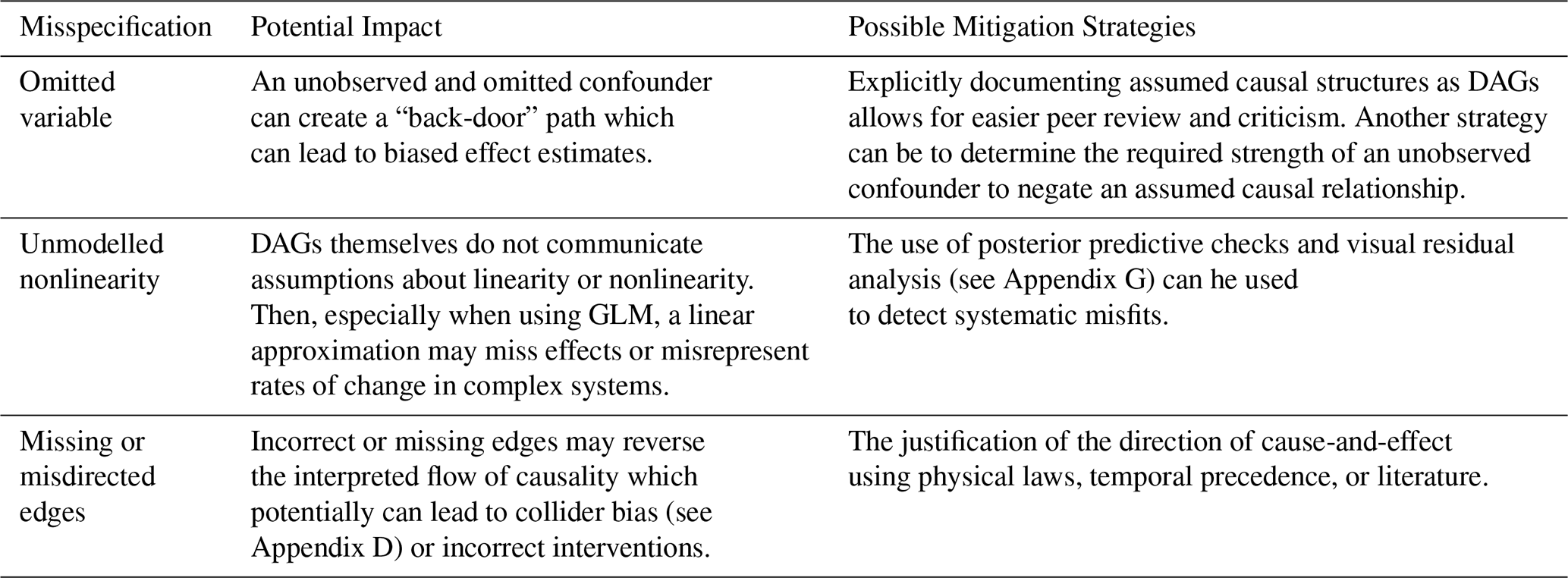
The causal framework in this study did not aim to discover previously unknown physical processes governing the formation of gaseous mercury in the oceans. Instead, the contribution lies in quantifying how known processes jointly contribute to observed variability under observational conditions outside of a laboratory. Specifically, using the suggested causal framework, it is possible to (i) separate total observed association between solar radiation and measured mercury into direct and temperature-mediated components, (ii) quantify the relative importance of these causal pathways, and (iii) adjust effect estimates for confounding influences such as environmental influences and instrument-intrinsic factors that are difficult to control in field observations. While laboratory and field experiments showed that solar radiation and sea surface temperature influence mercury emissions, the proposed causal framework allows these effects to be estimated simultaneously from observational data under explicitly and transparently stated causal assumptions. This causal inference technique therefore provides effect size estimates that are directly interpretable for large-scale modelling efforts or policy assessments, where controlled experiments may be infeasible. Causal conclusions, however, are conditional on the assumed causal models. DAGs, as graphical representations of causal knowledge, make prior causal knowledge explicit which allows other researchers to understand and criticise more easily the underlying assumptions. Such criticism is important because causal models are not immune to misspecification, such as by omitting unobserved but relevant confounders, leaving out, or misdirecting edges, which may lead to biased effect estimates. Table 5 lists a set of possible misspecifications and their mitigation strategies.

Table 5 Potential impacts of DAG misspecification and generalised mitigation strategies.

In the following, we revisit the research questions and summarise and discuss the answers we found and their implications for the mercury research community. Then, based on the findings and learnings from the case study, we discuss the use of causal inference in combination with prior knowledge in terms of its applicability to environmental research in general.

Answers to research questions

By applying the causal inference framework suggested in this paper, we found that solar radiation influences measured Hg concentrations in seawater both directly, and indirectly through its effect on sea surface temperature. We verified that the final model m₄, although being a simple model of the cause-effect relationships for Hg concentration in seawater, can reconstruct the probability density of the observed data adequately well with an R² value of 0.626. After adjusting for additional external influences (RQ2), we identified the following effect sizes:

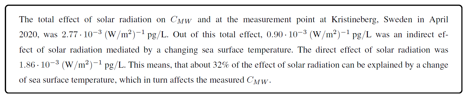
Box 8 Answer to RQ1 – What is the direct and indirect effect of solar radiation on measured Hg concentration in seawater?

We found that wind has a confounding influence on the effect estimates of solar radiation on C_MW, and that variations in pump speed significantly affect the measured gaseous Hg concentration, which is explained by Eq. (2). Accordingly, the additional causal modelling of wind as a confounder and pump speed as an instrument-intrinsic factor in model m₄ allowed us to adjust the total, indirect, and direct effects of solar radiation on measured mercury concentration in seawater:

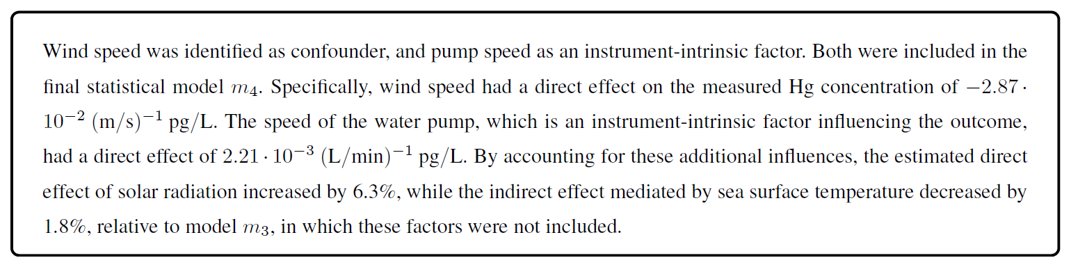
Box 9 Answer to RQ2 – What are the effect sizes of additional confounding and distributing factors affecting the measured Hg concentration in seawater?

6.2 Implications for future mercury research and policies

As mentioned in Sect. 1.1, several studies report an observed significant correlation between measured gaseous mercury and solar radiation. However, considering the regression only between these two factors results in a very simple model, comparable to our model m₁ (Fig. 4a). This model is not comprehensive enough to allow for drawing correct causal conclusions. In contrast, model m₄ (Fig. 5) explicitly incorporates both mediation by sea surface temperature (T_S), confounding by wind speed (W), and an instrument-intrinsic influence through the pump speed (r_W). The model is more reliable because it reduces bias from additional competing effects, confounders, and background conditions that, if ignored, would give a misleading picture of the underlying causal relationship. Figure 13 illustrates the practical implication of this difference. For an increase in solar radiation from 600 to 800  W m⁻², model m₁ predicts an increase in measured mercury of about 0.56 pg L⁻¹. In contrast, the causally adjusted model m₄ predicts a smaller increase of only about 0.42 pg L⁻¹. Thus, the estimated effect size of solar radiation on mercury emission is about 25 % lower if causal relationships are accounted for. In summary, if causal relationships are ignored, there is a risk of overestimating the effect of solar radiation on gaseous mercury.

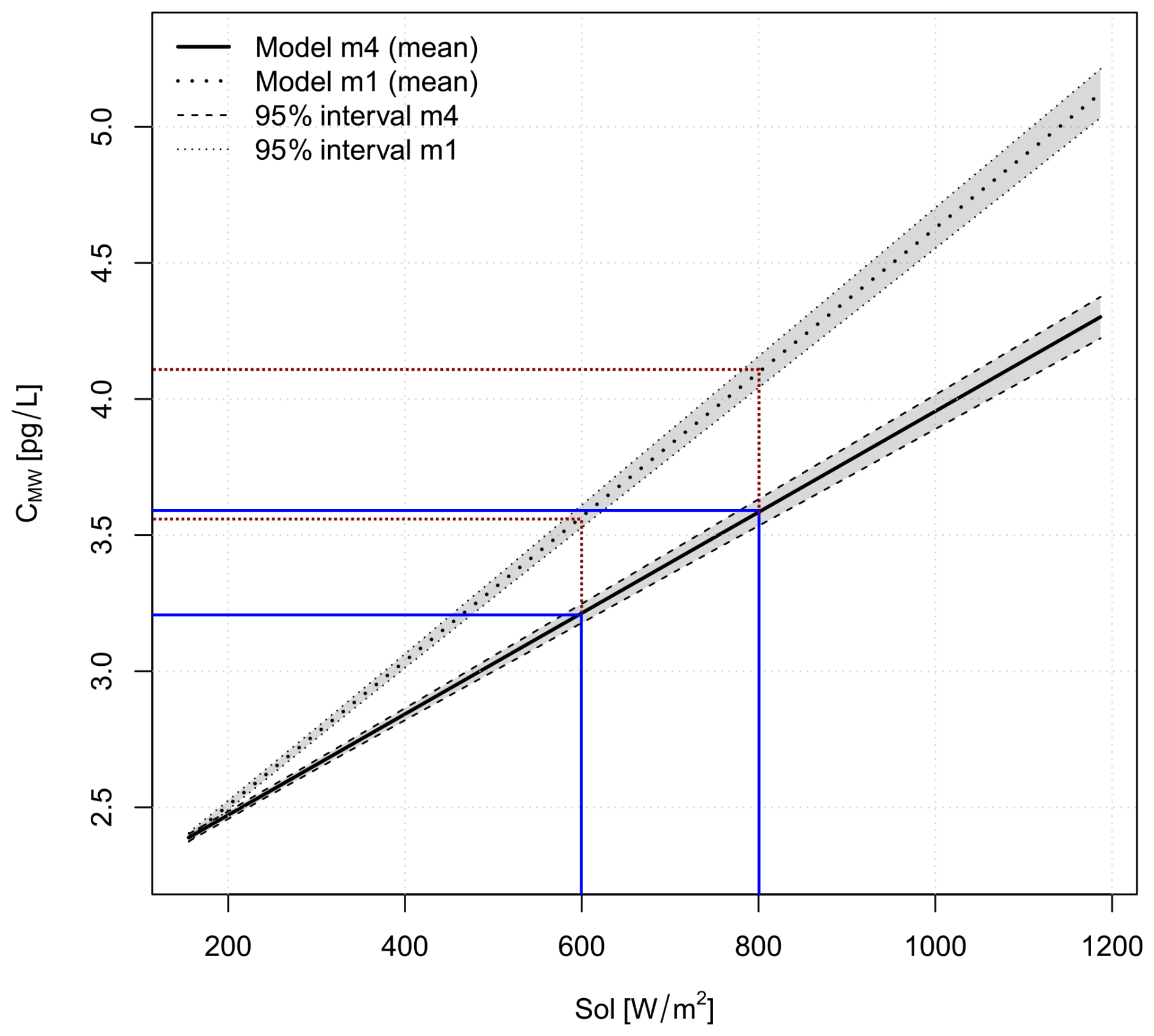
Figure 13 Comparison of posterior mean regressions of the effect of solar radiation Sol on mercury concentration C_MW using model m₁ (dotted line) and model m₄ (solid line). Grey shading indicates the 95 % confidence interval. Vertical reference lines at Sol = 600 and 800 W m⁻² are the solar radiation levels used to compare effect sizes between the models.

However, to succeed with the challenging task of evaluating for example the effectiveness of the Minamata Convention on Mercury (United Nations Environment Programme, 2024), better and more reliable computer models are needed to support sparse mercury measurements. Re-emissions of volatile mercury from sea surfaces is one of the largest contributors to the mercury load in the atmosphere, which is highly depending on the concentration of mercury. To build better computer models we need reliable predictors. One of our contributions towards finding more reliable predictors is showing the importance of modelling prior causal knowledge and including it in statistical models to correctly identify and connect competing and confounding factors to measured gaseous mercury. The use of graphical causal models strengthens reliability in the results because these models make the underlying causal assumptions transparent and guide the choice of which predictors to include in the regression analysis.

6.3 General implications for causal inference in environmental science

Previous attempts to apply causal inference in environmental research have often avoided using prior knowledge. Instead, they tried to discover causal relationships in time series using methods such as Granger causality tests (Runge et al., 2023), potential outcome framework (Reich et al., 2021), or by mimicking randomised controlled trials (Pearce and Lawlor, 2016). However, these approaches rely on strong and often non-transparent assumptions (Maziarz, 2015). Graphical causal models, on the other hand, allow to encode prior assumptions transparently such that the necessary restricting conditions for causal inference from observational data are provided. This does not mean that graphical causal models remove the need for prior assumptions, nor do they guarantee the correctness or completeness of prior causal knowledge. As with other causal frameworks, such as potential outcome frameworks or Granger causality, the validity of any causal claim depends on the underlying prior assumptions and the adequacy of the data. Other causal frameworks are not inherently “non-transparent” but they use different, and often more implicit, mechanisms to communicate prior assumptions such as exchangeability assumptions (Hernán and Robins, 2020) or stationarity requirements. In this sense, the primary contribution of graphical causal models is to offer a particularly explicit and inspectable representation of prior causal knowledge. The importance of defining prior causal knowledge as graphical causal models has been recognised in other scientific disciplines, such as medicine (Glass et al., 2013), economy (Imbens, 2020), social science (Imbens, 2024), and software engineering (Furia et al., 2019). Scientists in these fields proposed a set of different workflows to work with graphical causal models.

In addition to workflows developed in other disciplines, it is important to distinguish the proposed causal inference framework from conventional scientific modelling in environmental science. Scientific modelling aims to formalise the understanding of researchers into mathematical or computational models (physical, empirical, statistical, or hybrid) that generate verifiable predictions of system dynamics (Beven, 2018). Such models are calibrated and validated against observational data and progressively refined as new data becomes available. In these models, causal assumptions are embedded implicitly in functional forms and governing equations. In contrast, the primary aim of the causal inferences framework is not the predictive reproduction of system dynamics but the quantification of direct and indirect effect sizes under explicitly stated causal assumptions represented by graphical models. Similar to conventional modelling, parameter estimation and model evaluation are governed by real observational data. The two approaches therefore address complementary research questions. While scientific modelling aims to predict how a system behaves, causal inference aims to disentangle and quantify the causal contributions of different factors to observed outcomes.

Here, we propose a framework for causal inference using observational data in environmental research with three general elements:

1. First, we suggest incorporating prior knowledge about (assumed) cause-effect relationships in form of a DAG. If a researcher is uncertain about some of the cause-effect relationships, we proposed to define different possible causal models for a given scientific question. Based on mathematical operations that can be performed on the graphical models, known as d-separation (Pearl et al., 2016), independence criteria can be derived for each model. These independence criteria, applied on the observational data, can be used to provide evidence for the selection of one or several candidate causal models.

2. In a second element of the framework, further evidence is collected that show that the proposed statistical or ML models based on the selected causal models are plausible, workable, and adequate.

3. In a final element, the reporting of the results, we argue that the results of the analysis must not only include reporting on the inference outcome, i.e., the parameter estimates. The collection of evidence arguing for the models' plausibility, workability, and adequacy and the incorporated prior knowledge in form of graphical causal models should become a natural part of the result report as well. Only if the causal models that underpin the statistical analysis are available, peers can scrutinise the underlying prior assumptions and argue for or against the findings.

7 Conclusions

This study proposed and demonstrated a framework for estimating the effect sizes of multiple forcings on environmental outcomes using observational data. Our case study quantified the direct and indirect effects of solar radiation on measured gaseous Hg in seawater. We showed that 32 % of the total effect was mediated by sea surface temperature, and that wind and water pump speed acted as confounders. The results from the case study support a framework for inferring effect sizes of cause-effect relationships using observational data which is the key contribution of this study. The framework includes concise steps for integrating expert knowledge into causal models, validating these models against data, and reporting both statistical inference results and the assumptions underpinning them.

The results are relevant for environmental research in several ways: Today's statistical and even advanced ML models cannot identify and quantify causal relationships in observational data alone. Because we usually cannot conduct randomised controlled trials in environmental research to quantify causal relationships, we must use other methods to identify the strength of causal relationships. By using causal modelling as part of the analysis of observational data, researchers can explicitly include their prior domain knowledge and assumptions in the otherwise purely automatic statistical analysis of the data. This prior knowledge can be used to impose constraints on statistical models that allow researchers to quantify different effect sizes from observational data. Being able to distinguish between the effect sizes of different forcings on an observed outcome is important because it also allows to distinguish between direct and indirect effects, and thus the effect of future interventions on the environment. For example, because the final causal models and data suggest that sea surface temperature positively influences gaseous elemental Hg, we know that an increase in sea surface temperature, for example due to climate change, will accelerate the release of mercury and we can quantify this effect using explicit assumptions about causal relationships. In addition, providing prior knowledge in the form of graphical causal models as part of the results of a statistical analysis strengthens the validity of those results because the assumptions about cause-effect relationships made by the researchers are explicitly recorded and can be scrutinised together with the results of the statistical or ML models.

Limitations and further research

There are limitations to using causal models as a guide for inferring causal knowledge from observational data in environmental research. For example, we have shown that the results of causal inference can be highly sensitive to confounding factors, such as the presence of unmeasured external factors. Future research should explore how to inform future data collection by identifying sensitivity to unmeasured confounders using causal models. Furthermore, missing and noisy data should be explicitly modelled, as their causes may be entangled with the variables under study.

Another limitation of our approach is that independence criteria alone may not be sufficient to select a correct causal model for analysis. There are situations where several causal models may have identical independence criteria, and we cannot distinguish between them. Future research can explore how the proposed framework can be extended with causal discovery approaches to suggest candidate causal models (Spirtes and Zhang, 2016). We discussed earlier that current approaches to automatic causal discovery from observational data require too strong and non-transparent assumptions to be useful. However, combining automatic causal discovery with prior expert knowledge could be a promising approach.

Finally, the case study is limited by the limited amount of available data. In future research, it would be interesting to validate effect sizes using long-term measurements over several months or even years. Also, we only studied a few identified confounding factors. An improvement to this study could be to include for example measurements of dissolved organic carbon since this has been suggested to influence DGM concentration (Ferrara et al., 2003; Amyot et al., 1997).

Appendix A: Causal inference from observational data

When building predictive or analytical models using statistical methods, such as linear regression, or even advanced machine learning (ML) approaches such as deep learning (DL), the models learn associations between variables from observational data to infer properties of an underlying mathematical structure (Peters et al., 2017). Whether we use statistical modelling or advanced methods of ML, the learned underlying mathematical structure only allows us to identify associations between variables in the dataset which can then be used to build models for prediction and classification (Ghahramani, 2015). We learn the statistical dependence between variables in the observational data and then infer patterns and trends: for example, we learn that if X changes by 1 unit, on average, Y changes by 2 units, on average, and vice versa. However, statistical models cannot provide the direction of cause- and effect; we cannot infer the causal interdependencies of the underlying system (Runge et al., 2019). Is it X that causes Y to change, or is it Y that affects X? Reichenbach extended this problem to common causes: neither X nor Y could affect each other, instead there could be a third variable Z that is a common cause of both X and Y (Reichenbach and Morrison, 1956). Without additional information, the three cases X → Y, Y → X, and Y ← Z→ X cannot be distinguished using observational data and statistical modelling alone (Schölkopf, 2022). This limitation even applies to deep neural networks, whose opaque mode of operation usually does not allow the extraction of cause–effect relationships from observational data alone (Montavon et al., 2018).

Causal inference refers to the process of learning about causal relationships and the process of reasoning about outcomes of interventions and answering counterfactual questions. A common research design for inferring causal relationships are randomised controlled trials (RTC). In an ideal RTC, the subject under study is randomly assigned to different treatments (or effects of something), allowing researchers to isolate the effect of the treatment on the outcome of interest and thus identify and quantify average effect sizes (Hernán and Robins, 2020). This is a rigorous approach to evaluating causal relationships and allows, for example, the effectiveness of interventions to be assessed. Unfortunately, randomised experiments are often not possible due to prohibitive costs, ethical concerns, or other impracticalities of such experiments. Researchers in many fields, including environmental research, must therefore rely on observational data alone and find methods to infer causality. In environmental monitoring, the assignment of sampling times and sites to “unaffected” and “potentially affected” is not under the control of the researcher and therefore cannot be assigned at random (Stewart-Oaten, 1996). The author suggested that causal inference in environmental research only can be successful if there are diagnostic checks to exclude plausible causal models that do not fit the data, and measures of model uncertainty for those models that are not excluded. With beginning of the 2010s, political discussions are increasingly focused on the causes and effects of climate change and the impact of human activities on the environment. Environmental monitoring data are used to derive policies and conversation rules. One possible approach to extract knowledge about contributing factors to pollution is positive matrix factorisation (PMF) which is a factor analysis tool to judge the level of contribution of different factors to an outcome (Kyllönen et al., 2020). Sun et al. (2022) found that more than 1000 studies have been published using PMF as a tool to study source appointment for different environmental pollutants, whereof several have used it in mercury studies (Feng et al., 2022; Michael et al., 2016). PMF can be useful to explore latent patterns in data. However, it does not provide mechanisms for distinguishing correlation from causation. Causal modelling has been suggested to be a key aspect in evaluating the effects of environmental policies, such as laws, self-regulation of industry, or governmental oversight (Sills and Jones, 2018). The authors suggest that especially graphical modelling of cause-effect relationships using DAGs are useful to describe the potential effect of environmental policies.

Appendix B: Simulation of data and validation of causal models

Before applying the observed data to the models, we conducted a simulation study to validate that the proposed analytical models could correctly identify associations between the variables. This process involved generating simulated observations C_MW under three generative models $s_{m_{\mathrm{1}}}$ − $s_{m_{\mathrm{3}}}$, each representing different causal assumptions for the three prediction models m₁ − m₃. For the first dataset, $s_{m_{\mathrm{1}}}$, we assumed that only Sol but not T_S has an influence on the generated $C_{\mathrm{MW}}^{\left(\mathrm{1}\right)}$ data. For the second dataset $s_{m_{\mathrm{2}}}$, we assume that only T_S but not Sol influences $C_{\mathrm{MW}}^{\left(\mathrm{2}\right)}$. The last dataset $s_{m_{\mathrm{3}}}$ represents an influence of both Sol and T_S on $C_{\mathrm{MW}}^{\left(\mathrm{3}\right)}$. The datasets are generated using the following generative process:

$$\begin{array}{}\text{(B1)}& {\displaystyle }{s}_{\left(m_{\mathrm{1}}\right)}:C_{\mathrm{MW}}^{\left(\mathrm{1}\right)}\sim \mathcal{N}\left(a_C+b_{c,s}\cdot \mathit{\text{Sol}},\mathit{\sigma }\right)\text{(B2)}& {\displaystyle }{s}_{\left(m_{\mathrm{2}}\right)}:C_{\mathrm{MW}}^{\left(\mathrm{2}\right)}\sim \mathcal{N}\left(a_C+b_{c,t}\cdot T_{\mathrm{S}},\mathit{\sigma }\right)\text{(B3)}& {\displaystyle }{s}_{\left(m_{\mathrm{3}}\right)}:C_{\mathrm{MW}}^{\left(\mathrm{3}\right)}\sim \mathcal{N}\left(a_C+b_{c,s}\cdot \mathit{\text{Sol}}+b_{c,t}\cdot T_{\mathrm{S}},\mathit{\sigma }\right)\end{array}$$

In these models, the outcome $C_{\mathrm{NW}}^{\left(i\right)}$ is normally distributed with a mean including a constant term a_C. The parameters b_c,s and b_c,t represent the effect sizes of solar radiation and sea surface temperature, respectively. Standardised values were used for the predictors to avoid numerical issues. A standard deviation σ was assumed to introduce uncertainty. Table B1 list the values for the parameters of the simulation models that generated the test data.

Table B1 Parameters for the generative models to create the simulation datasets.

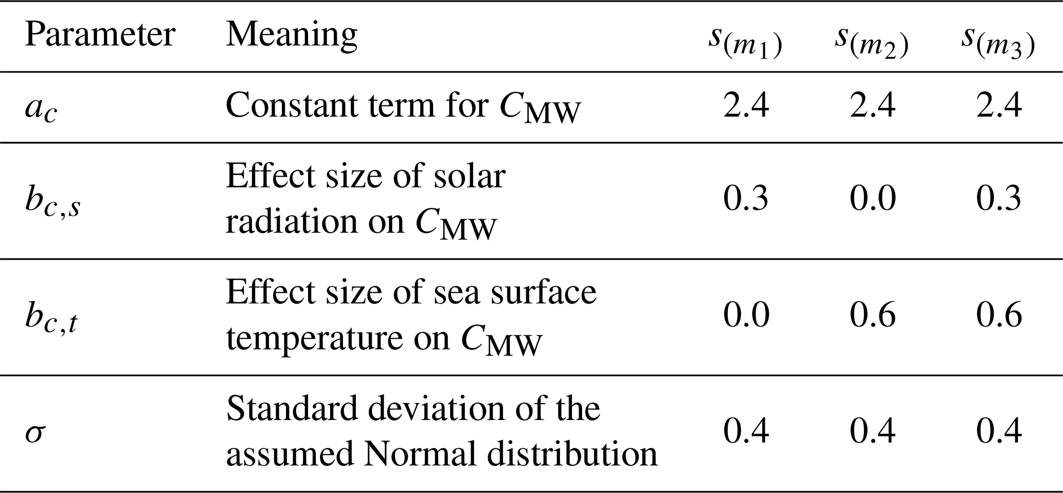
The interpretation is as follows: for model $s_{\left(m_{\mathrm{1}}\right)}$, setting b_c,s − 0.3 implies that a 1 standard deviation change in solar radiation leads to a b_c,s-times change in the simulated outcome. Similarly, model $s_{\left(m_{\mathrm{2}}\right)}$ with b_c,t − 0.6 implies a corresponding change due to sea surface temperature. Model $s_{\left(m_{\mathrm{3}}\right)}$ combines both effects. Figure B1 presents the resulting simulated data for $C_{\mathrm{NW}}^{\left(i\right)}$ under the three different causal assumptions.

We then performed Bayesian model inference using the three models on each dataset. The inference results are listed in Table B2 and visualised in Fig. B1.

Ideally, models should recover the original parameter values despite the added uncertainty σ = 0.4. Furthermore, we could examine what happens if we estimate the parameters using an incorrectly specified model for the dataset. For example, model m₂ assumes no causal relationship between solar radiation and C_MW, but the datasets $s_{m_{\mathrm{1}}}$ and $s_{m_{\mathrm{3}}}$ simulate such a causal relationship. Consequently, model m₂ incorrectly estimates b_c,t for these datasets, mapping effects from solar radiation to sea surface temperature. In these cases, the estimated σ also increases beyond 0.4 as the model fails to account for all variance in the data. By contrast, model m₃ correctly estimates zero effects for irrelevant variables under datasets $s_{m_{\mathrm{1}}}$ and $s_{m_{\mathrm{2}}}$ which indicates the ability to detect statistical independence consistent with expectations listed in Table 1.

Table B2 Parameter estimates for all models under simulated datasets $s_{\left(m_{\mathrm{1}}\right)}$, $s_{\left(m_{\mathrm{2}}\right)}$, and $s_{\left(m_{\mathrm{3}}\right)}$.

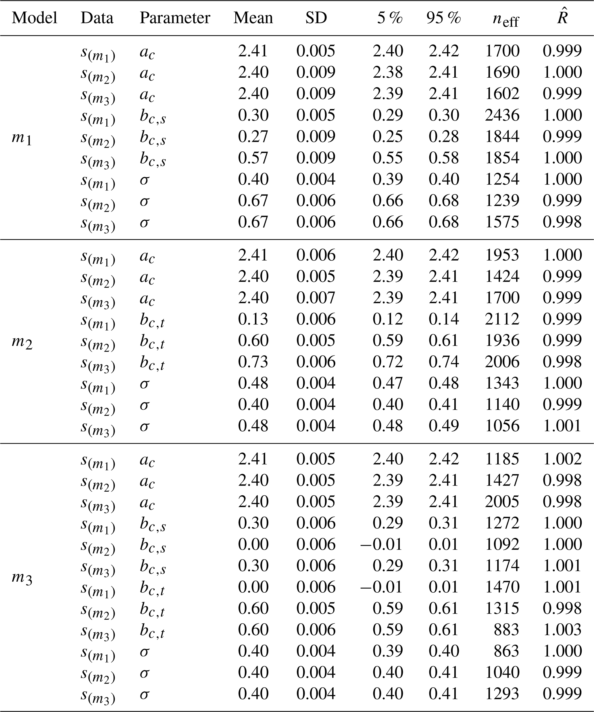
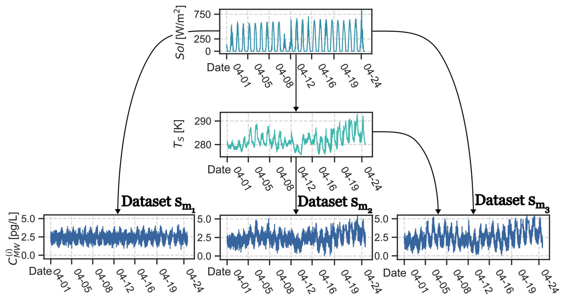
Figure B1 Resulting datasets $s_{m_{\mathrm{1}}}$ − $s_{m_{\mathrm{3}}}$ for simulated outcome $C_{\mathrm{NW}}^{\left(i\right)}$ under three different causal assumptions using observed solar radiation Sol and sea surface temperature T_S. Arrows indicate assumed direction of cause and effect.

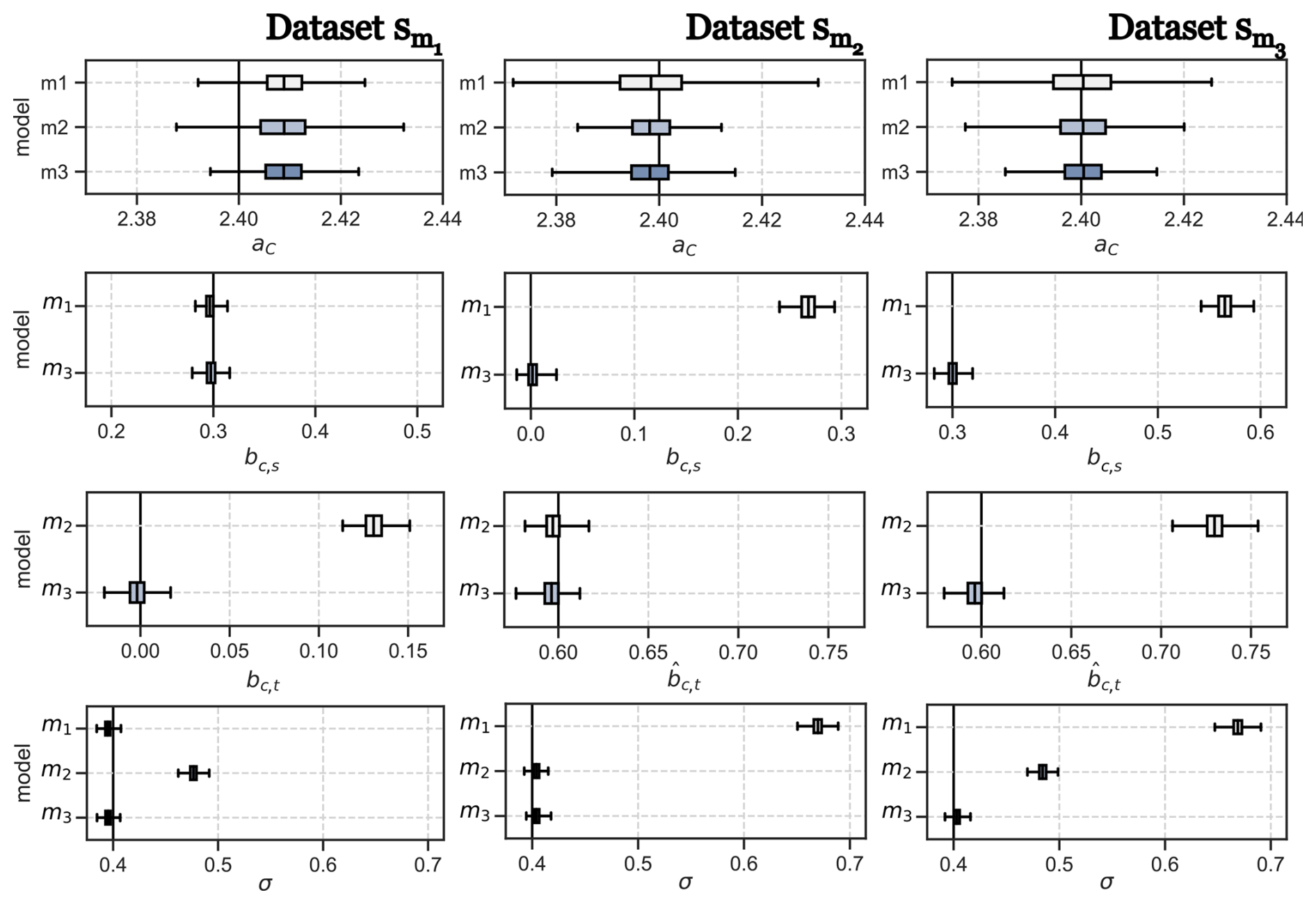
Figure B2 Results of model inference under three different simulated datasets $s_{m_{\mathrm{1}}}$ − $s_{m_{\mathrm{3}}}$, each representing different causal assumptions for C_MW. The left row shows inference under dataset $s_{m_{\mathrm{1}}}$, the middle row under dataset $s_{m_{\mathrm{2}}}$, and the right row under dataset $s_{m_{\mathrm{3}}}$. Solid black lines indicate the true parameter values set for the simulation.

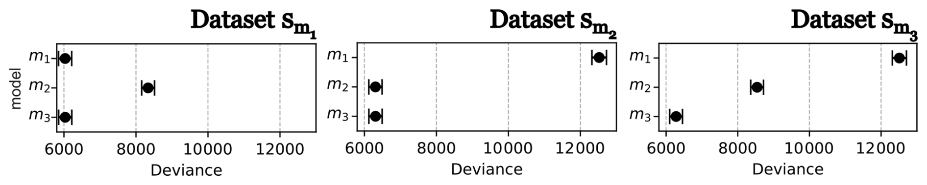
Figure B3 Model comparison using WAIC. Lower deviance values indicate that a model is more adequate for the data.

The WAIC-based model comparison, shown in Fig. B3 shows:

• For dataset $s_{m_{\mathrm{1}}}$: models m₁ and m₃ are adequate.

• For dataset $s_{m_{\mathrm{2}}}$: models m₂ and m₃ are adequate.

• For dataset $s_{m_{\mathrm{3}}}$: only model m₃ is adequate.

In conclusion, the results of the simulation study show that the models are workable, meaning that, given the chosen priors, they can infer an a priori determined set of parameters in simulated datasets. We saw that if a model does not by design allow for an association that is present in the dataset, the model will instead incorrectly “map” the missing association onto other allowed associations, which can inflate unrelated effect sizes. Finally, we saw that model m₃ can detect the non-existent of association between variables in the datasets. Paired with domain-derived independence criteria (Table 1), this allows making statements about possible causal relationships in observational data.

Appendix C: Prior predictive plots simulations

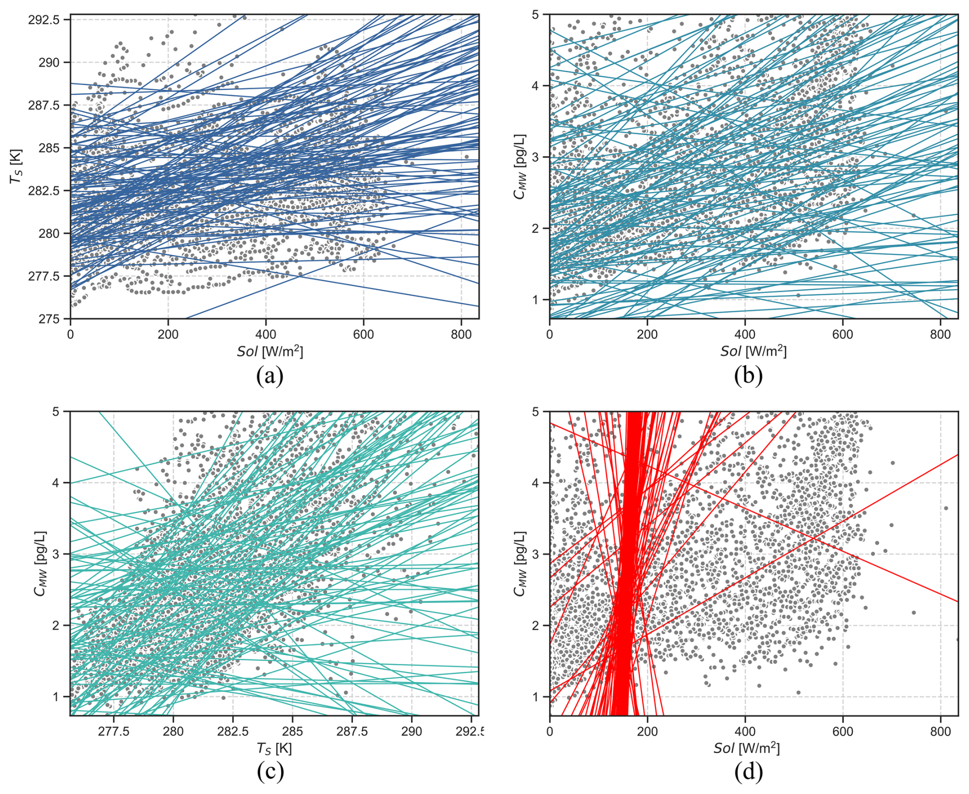
Figure C1 Prior predictive simulation results. The observed data is shown as grey circles. (a) $a_t\sim \text{Normal}(\mathrm{0},\mathrm{1})$, $b_{t,s}\sim \text{Normal}(\mathrm{0.5},\mathrm{0.5})$. (b) $a_c\sim \text{Normal}(\mathrm{2.7},\mathrm{1})$, $b_{c,s}\sim \text{Normal}(\mathrm{0.5},\mathrm{0.5})$. (c) $a_c\sim \text{Normal}(\mathrm{2.7},\mathrm{1})$, $b_{c,t}\sim \text{Normal}(\mathrm{0.5},\mathrm{0.5})$. (d) $a_c\sim \text{Normal}(\mathrm{2.7},\mathrm{1})$, $b_{c,s}\sim \text{Normal}(\mathrm{20},\mathrm{20})$, which is an example of an implausible prior.

Prior predictive plots assist in identifying reasonable initial values for the parameters of the prior distributions. This is done by simulating the model outputs solely using the priors (McElreath, 2020).

Because the predictor values are standardised, we set a_t = 0. The outcome variable C_MW, however, was not standardised, which is why we set the prior mean of a_c to 2.7, corresponding to the mean of the observed C_MW. These values are reasonable initial choices for a_t and a_c as both parameters represent intercepts of a linear regression. The prior predictive plots were then used to identify initial values for b_c,s,b_t,s, and b_c,t. Each plot in Fig. C1a–c shows 100 randomly drawn lines using models m₁ − m₄, with parameter values sampled from the corresponding priors. Observed data are shown as black circles.

Our aim was to choose the parameters of the prior distributions such that the simulation results obtained by sampling were plausible given the observed data. Figure C1d illustrates an example of an implausible prior distribution. It was not our aim to match the observed data precisely because priors only serve as a “starting point” for the Bayesian data analysis. The influence of the priors diminishes the more observational data are available as the model iteratively updates its estimates based on the data. Nonetheless, selecting reasonable priors improves the efficiency of inference by reducing the time required to estimate the posterior distributions.

Appendix D: A warning about colliders and uninformed machine learning (ML) models

A common approach might be to include all possible predictor variables in a statistical or ML model. However, a particular situation arises when colliders are part of the causal model. A collider is any variable with several causes affecting it. Figure D1 provides an example of a devised example based on the previous model m₃. Assume that variable A represents the particle density of algae in the water and that the growth of algae is positively affected by solar radiation. Assume also that mercury has some form of inhibitory effect on algae, which reduces the density of algae in waters with high mercury concentration.⁶ Variable A represents a collider in the causal model because it has arrows pointing towards it from both Sol and C_MW. One problem in causally interpreting the results of statistical or ML models that arises in the presence of colliders is collider bias. It entails an association between two variables that “flows” against the direction of cause and effect. For example, a researcher might try to build a statistical model that predicts the effect of solar radiation on C_MW. The researcher conveniently has data on the density of algae particles and assumes that, because algae growth is affected by both solar radiation and Hg concentration, it is a good predictor for C_MW. We extended the previous simulation model $s_{m_{\mathrm{3}}}$ with a variable A depicting simulated algae growth that depends on solar radiation and C_MW to illustrate the consequence of including a collider as a predictor for estimating the effect size of solar radiation on C_MW.

Table D1 lists the parameters of the new simulation model $s_{m_c}$. By setting b_a,s = 0.7, we assume that solar radiation has a strong positive effect on the concentration of algae. Conversely, by setting b_a,c = −0.2, we assume a weakly negative effect of the presence of mercury on the concentration of algae. All other parameters are identical to those in simulation model $s_{m_{\mathrm{3}}}$ as given in Table B1.

Variable A is included as predictor of C_MW by extending model m₃ to a new statistical model, m_c, specified in Table D2.

Table D1 Added parameters to $s_{m_{\mathrm{3}}}$ for the generation of an extended dataset $s_{m_{\mathrm{3}}}$ that includes a collider A.

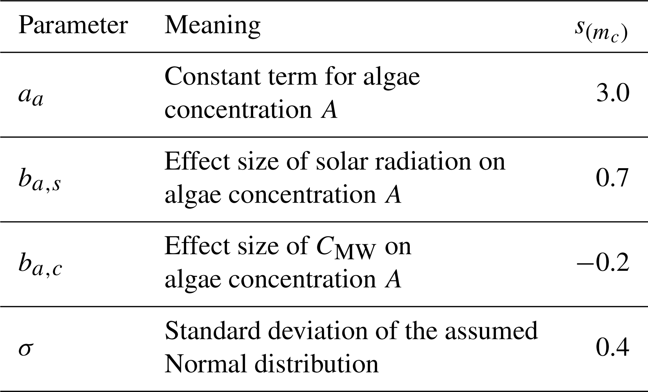
Table D2 Model specification for collider model m_c.

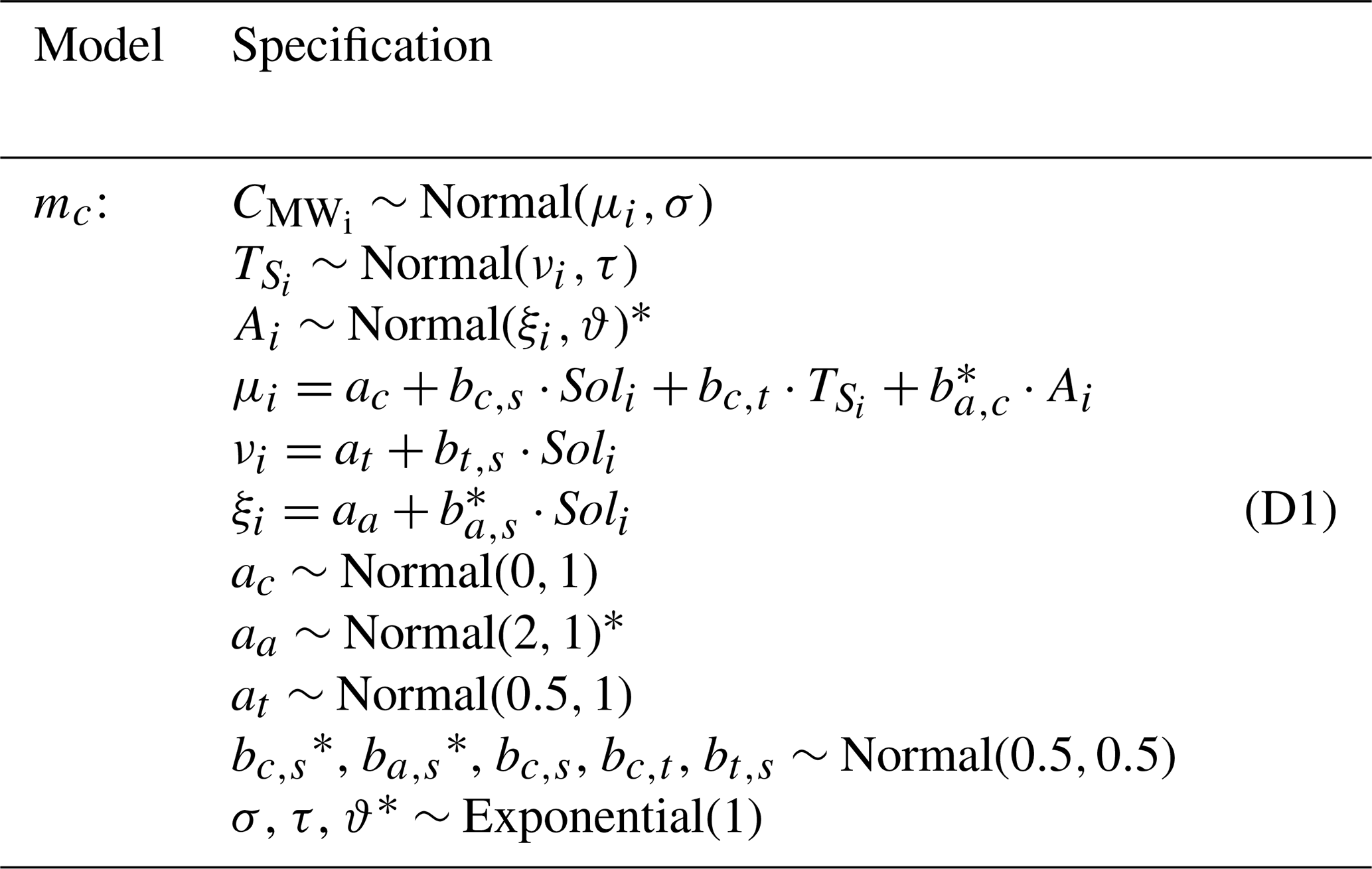
^*Terms that relate to algae growth A.

The inference results for model m_c are presented in Table D3 together with the previous results from model m₃.

Table D3 Parameter estimates for models m₃ and m_c under simulated data $s_{m_c}$. Bold faced values indicate the changed effect size of solar radiation on C_MW due to collider bias.

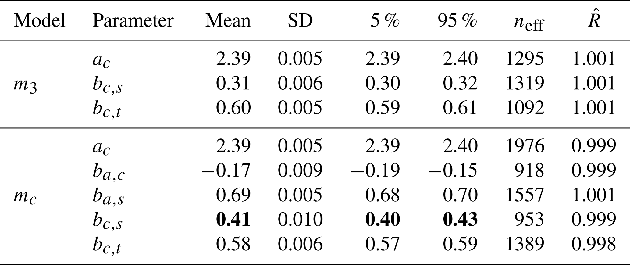
The new model correctly estimates the simulated effect sizes for algae density b_a,c and $b_{a_s}$. If not conditioned upon, colliders act as “sinks” for the flow of association (Holmberg and Andersen, 2022). That is, the “flow” of association between Sol and C_MW via A will be stopped by the collider variable A if we do not control for this variable. However, by including algae as a predictor for C_MW, the model inadvertently conditioned on a collider. Thereby, a collider bias is introduced in the estimate of the effect size of solar radiation on C_MW because additional association “flows” against the correct direction of cause-and-effect. Therefore, the effect size of solar radiation on C_MW, b_c,s, changes from its true value of 0.3 to a higher value of 0.41 to compensate for the additional “anti-causal” association flowing via A. In addition, the uncertainty in the effect size estimate b_c,s increases as illustrated in the larger bars in Fig. D2a.

Unfortunately, including additional predictors that are correlated with C_MW increases the predictive ability of the model as shown in Fig. D2b. This means that model m_c can predict C_MW better, even if the effect size estimates (the causes to why C_MW changes over time) are not correct. The danger is that when using ML model, the algorithm may include all predictor variables that it can find in the data. The result will be a model that predicts the outcome variable very well, but the effect sizes may be wrong. It is therefore important to carefully argue, using causal modelling for example, which variables to include in a dataset for ML, leading to an informed ML. Otherwise, conventional ML approaches, including advanced approaches such as convolutional deep neural networks, might inadvertently condition on collider variables and estimate incorrect effect sizes (Hernán and Robins, 2020).

Figure D1 Directed Acyclic Graphs (DAGs), which contains a collider A.

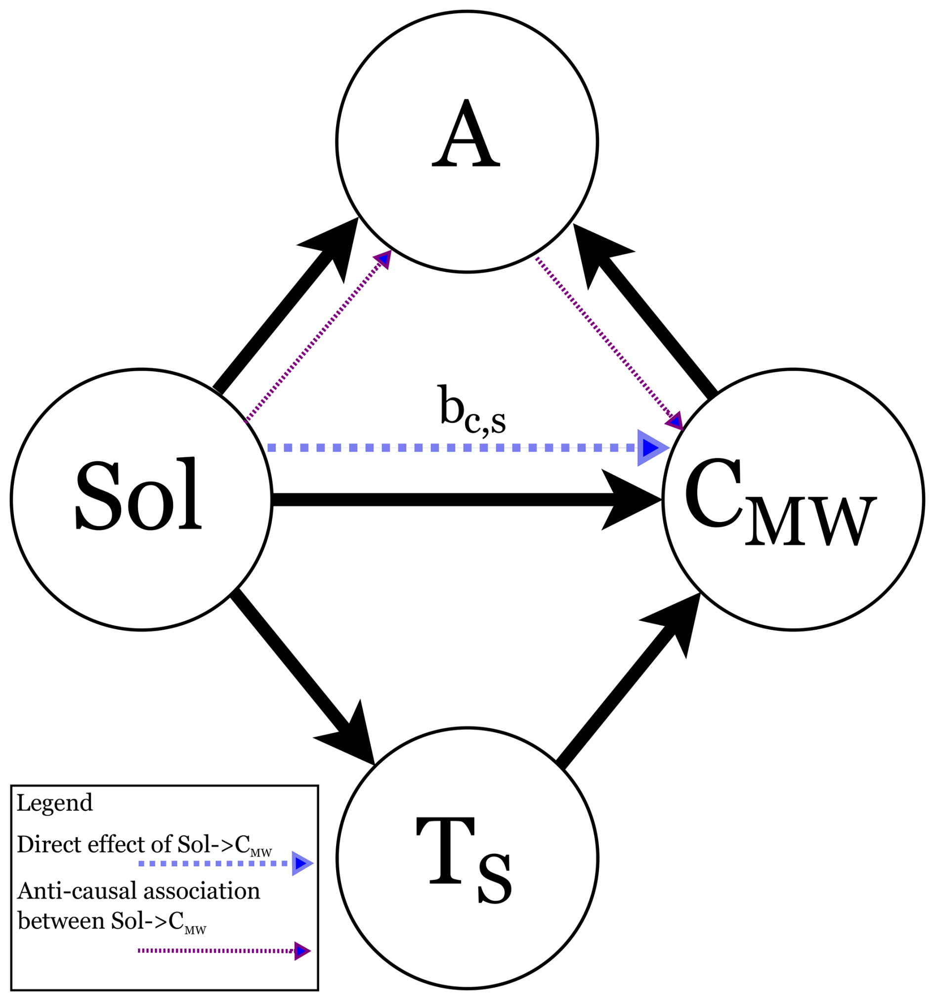
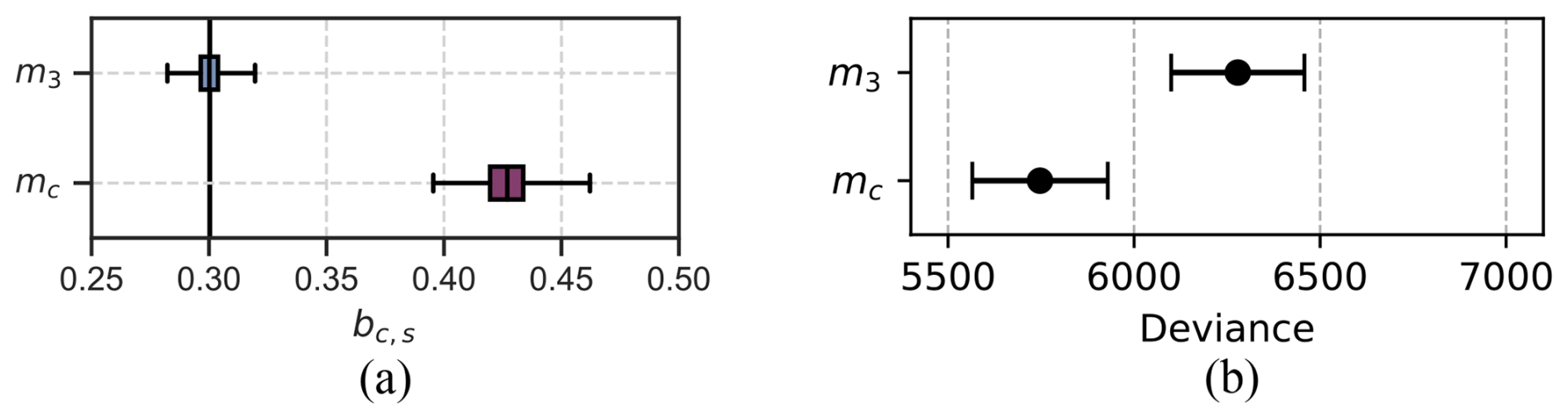
Figure D2 Estimate of effect size Sol → C_MW (a) and model comparison (b) for model with Algae growth A as predictor (m_c) and without A as predictor (m₃).

Appendix E: Validation through independence checking using scatterplots

E1 Independence checking

In addition to assessing the estimated effect size coefficients to evaluate independence between variables, we also conducted a manual inspection of scatter plots to visually assess statistical independence between the predictor variables and the outcome. Figure E1 presents the scatter plots corresponding to the independence criteria outlined in Table 1. For example, if C_MW were conditionally independent of solar radiation given sea surface temperature, as suggested by model m₁, we would expect no apparent pattern or trend between T_S and C_MW at different levels of Sol. However, Fig. E1a indicates a linear relationship between T_S and C_MW at each level of Sol. Similarly, Fig. E1b indicates a linear relation between Sol and C_MW which appears to be more distinct with higher values for T_S. Overall, the visual inspection of the scatter plots suggests that statistical independence between the variables is not supported, implying that the assumed causal models m₁ and m₂ are not plausible.

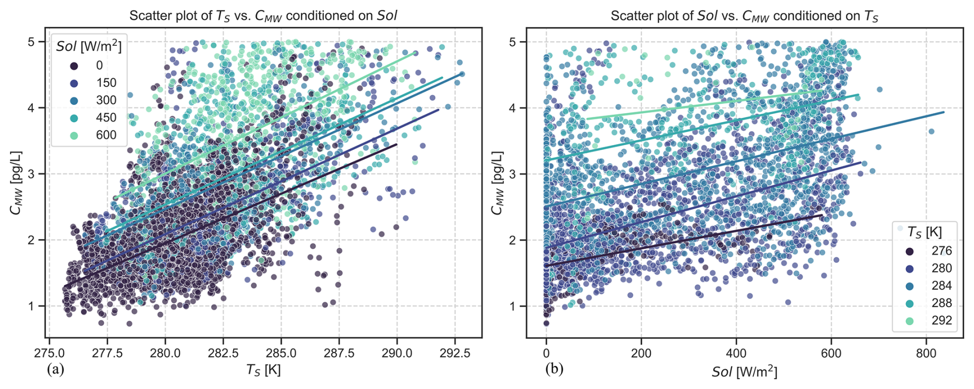
Figure E1 Scatter plots for inspecting suggested independence between variables for (a) m₁: T_S ⟂ C_MW∣ Sol and (b) m₂: Sol ⟂ C_MW∣T_S.

Appendix F: Parameter estimates under observed data

Table F1 lists the inference results using models m₁, m₂, m₃, and m₄ under the observed data.

Table F1 Parameter estimates for all models under observed data.

Appendix G: Discussion on the distributional assumption for C_MW

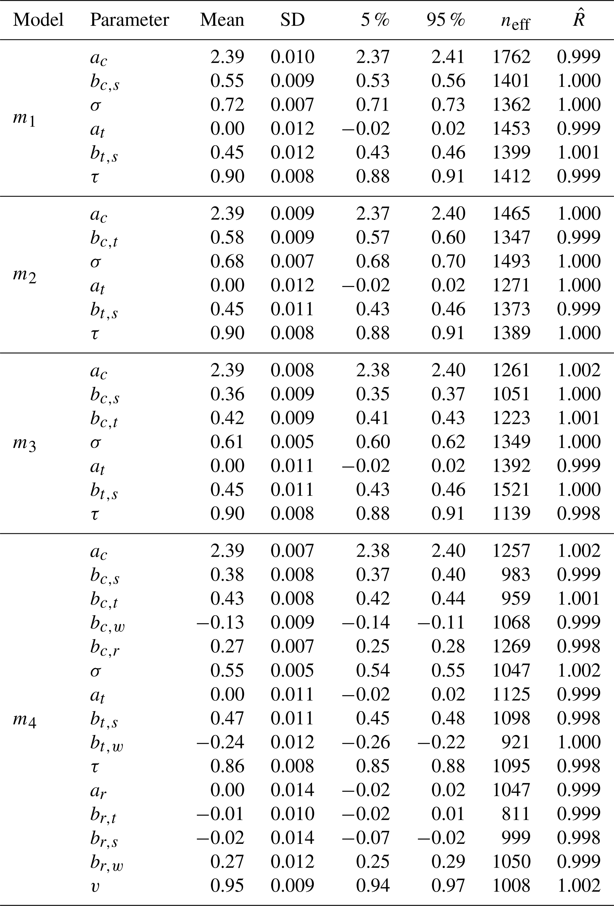
While assuming that the outcome data is normally distributed can be sensible in many cases, environmental data may show a multiplicative and right-skewed character which may also be indicated in the long-tail distribution of the observed C_MW data shown in Fig. 11e. In order to check if the normal likelihood assumption is appropriate for C_MW, we plotted the residuals of model m₄ against its fitted values. The resulting residual plot visualises the predication error between each observation and the model's estimate. If the assumption of normal distributed data for C_MW holds, the residuals will be symmetrically distributed around zero with a more or less constant spread. However, the plot in Fig. G1 suggests that the spread of the residuals is not constant but instead widens as the predicted C_MW increases, indicating that the model's error scales with the magnitude of C_MW. This pattern would justify the adoption of a Log-Normal likelihood which, unlike the Normal likelihood, models a multiplicative and long-tailed distribution nature of C_MW.

.

Figure G1 Residual plot which shows the prediction error against the predicted C_MW

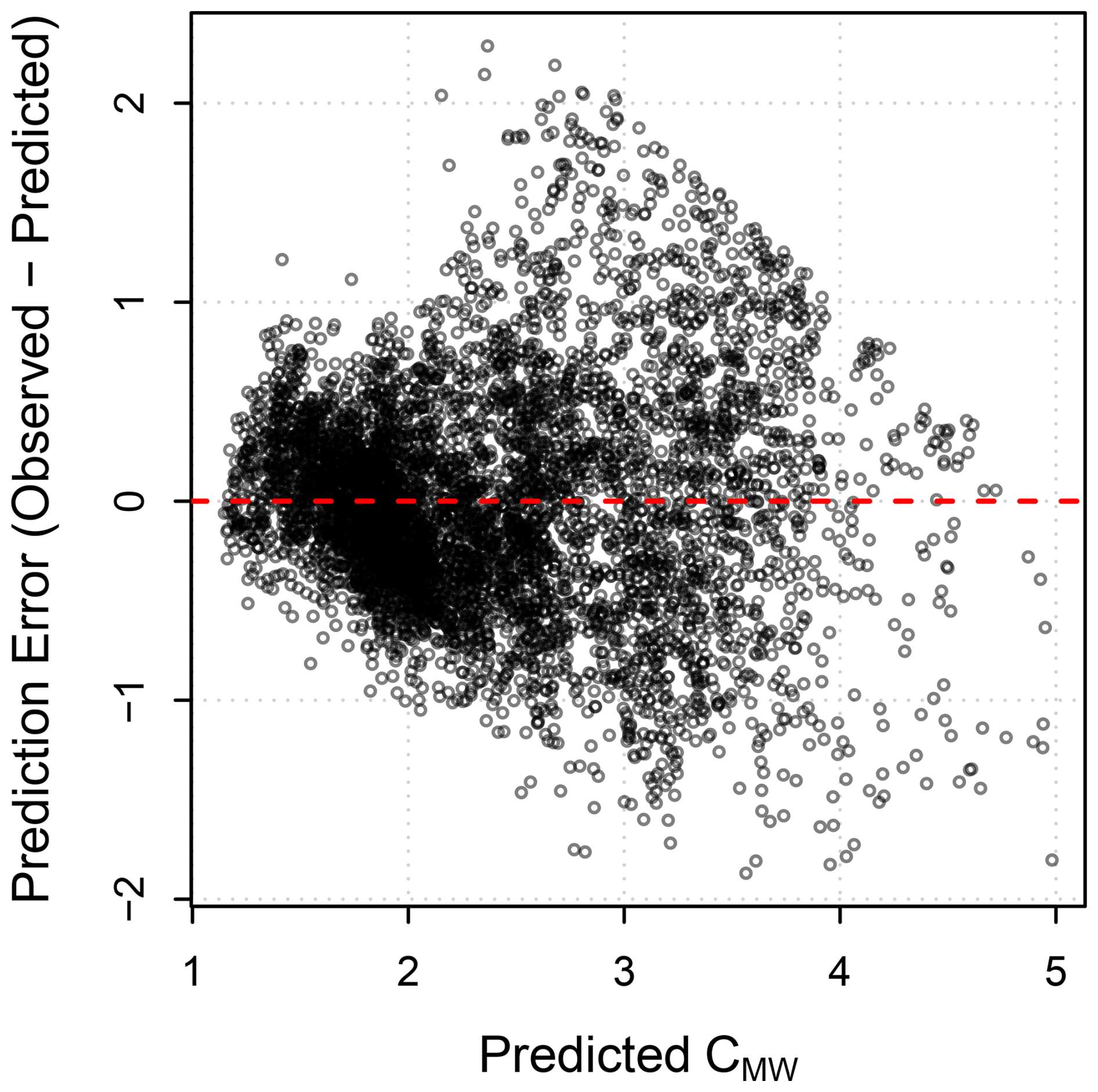
Modified model m₄ with log-normal likelihood

As we cannot conclusively exclude the appropriateness of a Log-Normal likelihood for C_MW, we modified the likelihood of model m₄ listed in Table (2) Eq. (9) to

$$\begin{array}{}\text{(G1)}& C_{{\mathrm{MW}}_i}\sim \text{Log-Normal}\left({\mathit{\mu }}_i,\mathit{\sigma }\right).\end{array}$$

This modification provides a new model $m_{\mathrm{4}}^{\log }$ and it entails that the linear predictor equation for μ_i now defines the mean on the log-scale. Although the mathematical notation of the equation does not change, the interpretation of the coefficients b_c,s, b_c,t, b_c,w, and b_c,r is now on a logarithmic scale which needs to be considered when comparing effect sizes later. Similarly, the priors are now applied to multiplicative effects. However, as we use weakly informative priors together with a large number of observations, the specific choice of prior scale is less critical for the posterior estimates.

Table G1 lists the resulting parameter estimates. To compare the parameter estimates thge table also lists the implied effect size for each predictor. This allows us to compare the parameter estimates even if the models use different mathematical scales. We calculated the implied effect size for the normal model as a percentage of the mean concentration, given by a_c:

$$\begin{array}{}\text{(G2)}& \text{Effect}\left(\mathit{\%}\right)={\displaystyle \frac{b_{c,\cdot }}{a_c}}\cdot \mathrm{100}.\end{array}$$

For the Log-Normal model, which is not additive but multiplicative, we calculated the implied effect size for each parameter by directly using the exponential function:

$$\begin{array}{}\text{(G3)}& \text{Effect}\left(\mathit{\%}\right)=\left(e^{b_{c,\cdot }}-\mathrm{1}\right)\cdot \mathrm{100}.\end{array}$$

The comparison suggests that although the log-normal is mathematically more rigorous, it has a very small effect on the parameter estimates, suggesting that the Normal assumption is a sufficient approximation for the data and that therefore the scientific conclusions regarding the effect sizes for mercury concentration are robust to the choice of likelihood. This robustness to the choice of the likelihood may stem from the small standard deviation compared to the average value for the concentration data (Limpert et al., 2001).

Table G1 Comparison of estimated parameters for C_MW between the Normal (m₄) and Log-Normal ($m_{\mathrm{4}}^{\log }$) models. The parameters are standardised. The implied effect is the change in % in C_MW per 1 SD increase in predictor.

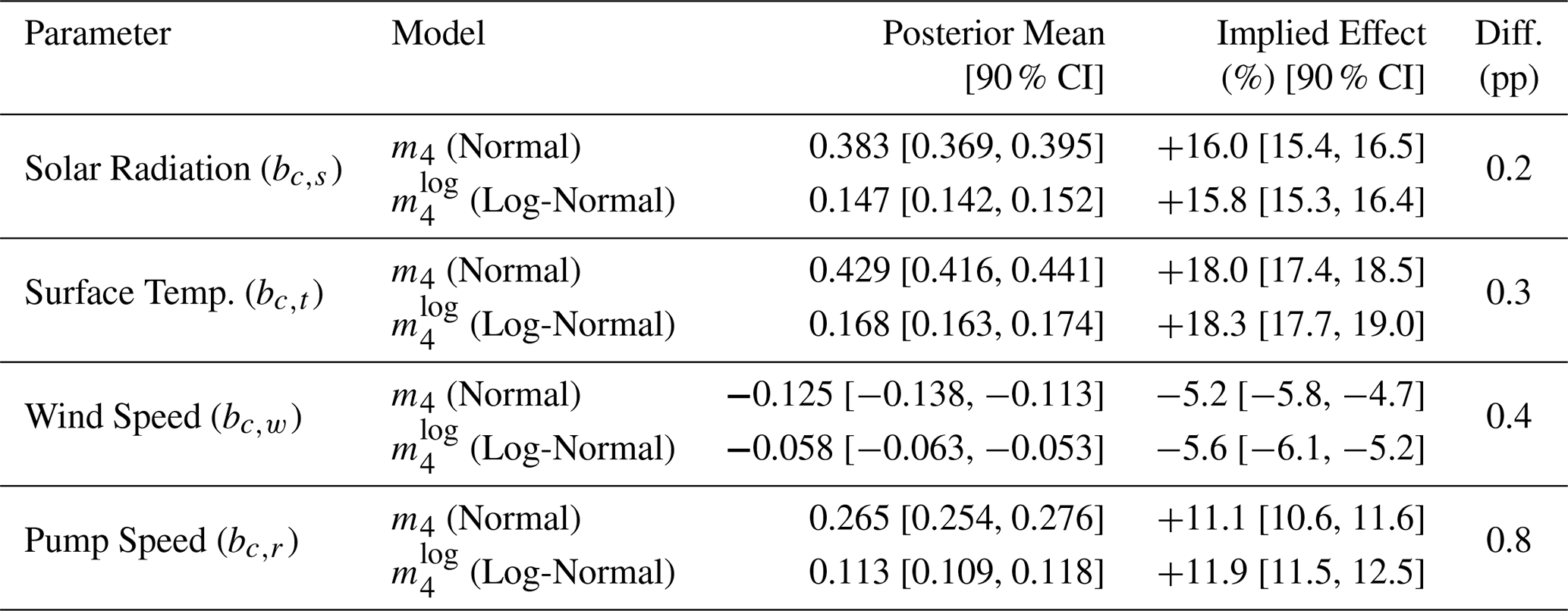
pp denotes percentage points. Implied effects for m₄ are approximate based on mean C_MW ≈ 2.39.

Appendix H: Workability: Assessing the convergence under Bayesian MCMC

We conducted Bayesian inference using a Markov Chain Monte Carlo (MCMC) sampling approach with Hamiltonian Monte Carlo implemented in Stan (Stan Development Team, 2024) using the rethinking interface by McElreath (2020). We assessed convergence using both quantitative diagnostics, including $\widehat{R}$ and the effective samples size (ESS/n_eff) as well as visual diagnostics, following standard recommendation for Bayesian workflows (Vehtari et al., 2021; Reich and Ghosh, 2019). First, the $\widehat{R}$ values for all parameters were close to 1 and < 1.01 as reported in Table F1. Second, all parameters have effective sample sizes (ESS/n_eff) exceeding 10 % of the total sample sizes which we assume sufficiently large (see Vehtari et al., 2021 and Furia et al., 2022 for a discussion on the sufficient ESS for BDA). Finally, we visually inspected the trace plots to verify adequate mixing, absence of strange divergent behaviour and stationarity. The trace plots are provided in Fig. H1 and show no indication of non-convergence such as slow trends, chain separation or autocorrelation. Together, these diagnostics provide evidence that the MCMC chains converged.

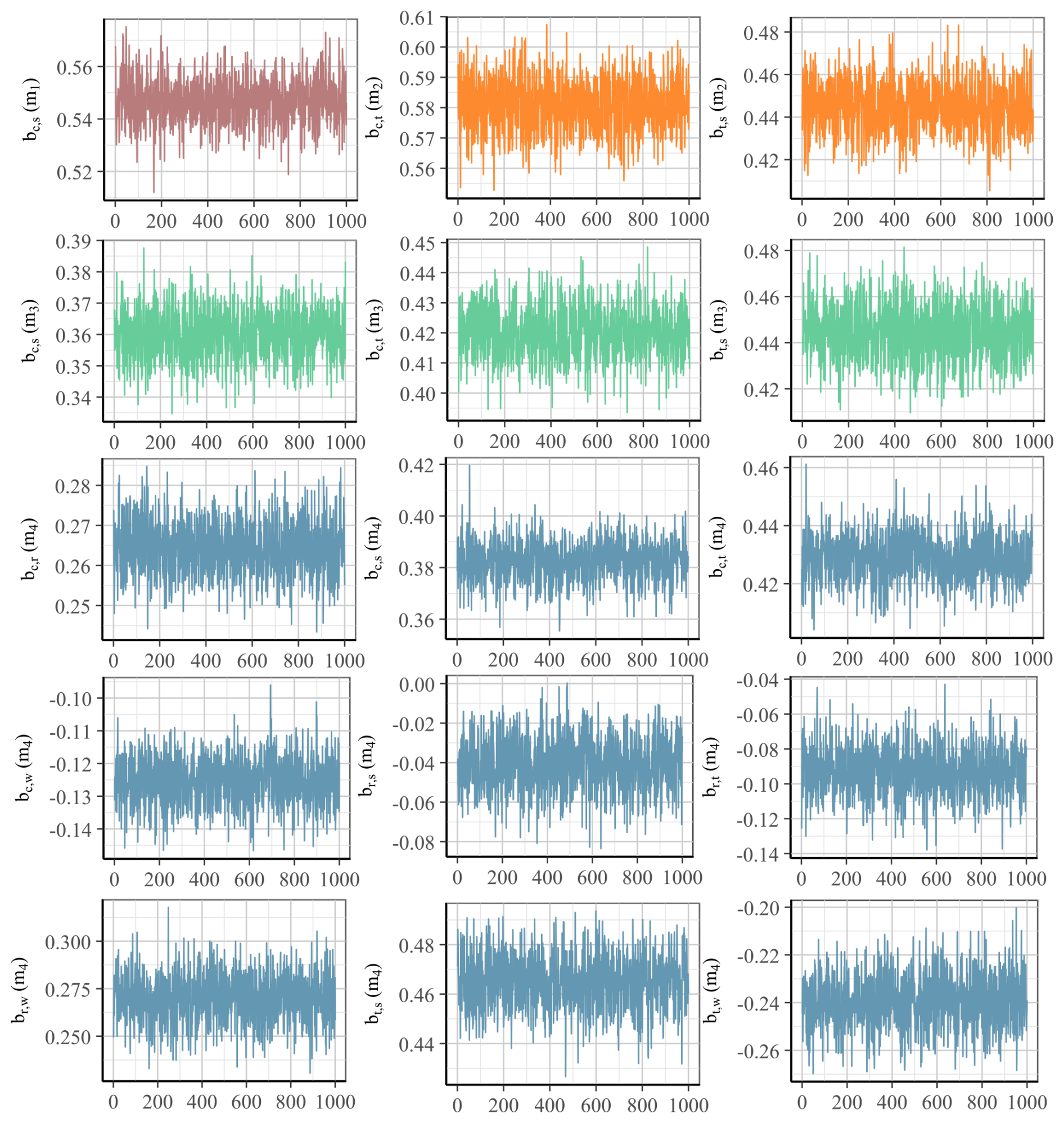
Figure H1 Trace plots for all effect size parameters of models m₁ (red), m₂ (orange), m₃ (green), and m₄ (blue).

Appendix I: Glossary of terms from causal inference and mercury chemistry

I1 Causal inference related terms

Causal inference	is the estimation of effect sizes under explicit assumptions about the causal structure underlying the data.
Causal models	are an explicit specification of assumed cause-effect relationships between variables in the data.
Confounder	is a variable that causally influences both an exposure and an outcome of interest which can lead to biased effect estimates.
Conditional independence	is the independence between two variables given a third variable.
d-separation	is a graphical method on DAGs for deriving conditional independence relations from a causal model.
Directed acyclic graphs (DAGs)	are a graphical representation of a causal model in which nodes represent variables and directed edges causal directions.
Direct effect	is the component of an effect that is represented by a direct causal path between two variables.
Indirect effect	is the component of an effect that is mediated by one or more intermediated variables.
Total effect	is the sum of direct and indirect effects.

I2 Mercury related terms

Dissolved gaseous mercury (DGM)	is gaseous mercury species dissolved in water.
Elemental mercury (Hg0)	is the volatile, gaseous form of mercury.
Measured gaseous mercury (CMW)	is the concentration of elemental mercury measured in the gas phase extracted from seawater.
Mercury evasion	is the emission of elemental mercury from seawater into the atmosphere.
Sea surface temperature (TS)	is the temperature of surface seawater at the influx to the measurement device.
Solar radiation (Sol)	is the incoming radiation from the sun measured at the experiment side.