Three-dimensional hollow tubular structure of rocket chemical depletion

The rocket launch process causes a series of disturbances in the ionosphere, among which a typical phenomenon is the formation of ionospheric electron density depletions caused by chemical reactions involving rocket exhaust, known as Holes in the Ionosphere from Rocket Exhaust (HIREs). Current research on the HIREs mainly focuses on the horizontal features observed from ground-based GNSS data. By utilizing COSMIC radio occultation data, we clearly observed the vertical structure of HIREs following the launch of an ATLAS-V rocket from Cape Canaveral Air Force Station on 22 May 2014. Additionally, combining ground-based GNSS, Swarm satellite observations, and numerical simulations, we delineated, for the first time, the three-dimensional “hollow tube” structure of the HIREs. Then, the spatiotemporal evolution of the HIREs is analyzed, and considered to mainly consist of three stages: “rapid formation, diffusion-driven growth, and diffusion-driven recovery”. The study contributes to a deeper understanding of the formation and development of artificial ionospheric plasma hollow-tubes.

1 Introduction

During rocket launches, the ionosphere undergoes a range of physical and chemical interactions, resulting in various disturbances. Rockets traveling at supersonic speeds through the mesosphere, alongside the explosive release of exhaust gases, generate shock waves and Atmospheric Acoustic-Gravity Waves (AGWs) (e.g., Arendt, 1971; Noble, 1990; Jacobson and Carlos, 1994; Li et al., 1994). These disturbances induce traveling ionospheric disturbances (TIDs), which are frequently observed within a certain range along the rocket's trajectory and have been extensively documented (e.g., Kakinami et al., 2013; Lin et al., 2017a, b; Chou et al., 2018; Yasyukevich et al., 2024). The rocket's propulsion relies on rapidly ejecting large volumes of combustion products, part of which are released into the atmosphere and can impact climate and stratospheric ozone (Barker et al., 2024). As the rocket ascends into the ionosphere, these exhaust gases expand rapidly in the ionosphere, they act like a “snowplow”, pushing background plasma outward and forming a density pile-up layer (e.g., Booker, 1961; Mendillo, 1988). Simultaneously, the exhaust pressure drops sharply to match the background ionosphere, transitioning into a free diffusion process. This exhaust, rich in H₂O, H₂, and CO₂, undergoes a series of chemical reactions during diffusion, further depleting ionospheric electrons and forming ionospheric electron density “holes” known as rocket-exhausted depletions (REDs) (e.g., Mendillo et al., 1975, 2008; Bernhardt et al., 2001). These chemical reactions produce excited oxygen atoms (O(¹D)) and hydroxyl radicals (OH), which emit 630 nm red light and 135.6 nm ultraviolet emissions, observable by airglow imagers, sounding rockets, and satellite instruments (e.g., Yau et al., 1985; Mendillo et al., 2008; Liu and Shepherd, 2006; Park et al., 2022).

REDs were first detected by sounding instruments (Booker, 1961) and through Faraday rotation of satellite signals (Mendillo et al., 1975; Wand and Mendillo, 1984). Subsequent studies primarily relied on GNSS-TEC data to capture the 2D horizontal distribution of REDs (e.g., Mendillo et al., 2008; Furuya and Heki, 2008; Nakashima and Heki, 2014). Furthermore, Park et al. (2015, 2016, 2022) observed associated electron density depletions using in situ satellite measurements even 6 h after the rocket launch, and captured 2D depletion distributions using satellite ultraviolet spectrometers. Numerous observations indicate that REDs typically emerge around 5–7 min after launch, persisting for 0.5 to 6 h (e.g., Bernhardt et al., 2001; Mendillo et al., 2008; Nakashima and Heki, 2014; Park et al., 2016). The depletion regions generally extend laterally along the rocket's trajectory, with widths of approximately 300–500 km and lengths exceeding 2000 km (e.g., Liu et al., 2018; Ozeki and Heki, 2010; Mendillo et al., 2008; Zhao et al., 2024). Inside REDs, total electron content (TEC) drops by 3–22 TECU compared to the background ionosphere (e.g., Liu et al., 2018; Park et al., 2022; Zhao et al., 2024), while maximum electron density reductions range from 20 % to 95 % (e.g., Furuya and Heki, 2008; Park et al., 2016; Wand and Mendillo, 1984; Mendillo et al., 2008; Zhao et al., 2024).

Current REDs observations largely rely on GNSS-TEC data, with a few nighttime launches observable through optical imaging (e.g., Mendillo et al., 2008; Park et al., 2022), which mainly capture horizontal 2D structures. Vertical structure observations remain scarce. A limited number of studies using incoherent scatter radar (e.g., Wand and Mendillo, 1984; Bernhardt et al., 1998, 2012; Zhao et al., 2024) have captured vertical profiles of REDs. Zhao et al. (2024) reported observations of ionospheric REDs structure during two rocket launches, and the results showed that REDs can extend to ∼200–700 km in altitude. The maximum depletion altitude for the afternoon event is 425 km, and the maximum depletion altitude for the midnight event is 283 km. Park et al. (2015, 2016) detected REDs diffusing to satellite orbit heights (450 and 518 km) through Swarm satellite in situ measurements. Park et al. (2022) also utilized the GOLD imager, Madrigal TEC, and multiple Low-Earth-Orbit satellites, with COSMIC-2 data suggesting an increase in ionospheric slab thickness at the depletion center, which may indirectly support the presence of vertical structural features. Meanwhile, the COSMIC-2 Gridded Ionospheric Specification (GIS) product offers some insight into the three-dimensional distribution of electron density depletions. However, given the relatively limited spatiotemporal resolution of the GIS data (5°×2.5° in latitude and longitude, with a temporal resolution of 1 h), which is somewhat coarse compared to the typical width (∼500 km) of REDs, it remains challenging to fully resolve the fine three-dimensional structure and evolutionary process of these features.

In this study, we obtained clear observations of the vertical structure of REDs using COSMIC-1 occultation data. Combining multi-source observations from COSMIC-1, Swarm satellites, and ground-based GNSS, we revealed the 3D hollow-tube structure of REDs and their evolutionary characteristics, offering a new perspective on rocket launch ionospheric disturbances. Additionally, high-resolution 3D simulations further validated the feasibility and reliability of the depletion modeling.

2 Data and simulation

2.1 Rocket launch event

Event-1: on 22 May 2014, an Atlas-V Rocket was launched from Cape Canaveral Air Force Station by United Launch Alliance (ULA) at 13:09 UT. Event-2: on 20 May 2015, a similar Atlas-V was launched at the same station by ULA at 15:09 UT. REDs from two launch events were reported by Park et al. (2016) using satellite in situ observations. This study primarily focuses on Event-1, while Event-2 serves as a supplementary case to provide horizontal observational data where Event-1 lacks coverage. Detailed trajectories of these two launches were not available; therefore, we derived the trajectories based on the rocket depletion observations by Park et al. (2015, 2016) and the Atlas-V user manual, as depicted in Fig. 1c. The launch information and Atlas-V user manual can be accessed from the ULA website: https://www.ulalaunch.com/missions (last access: 1 April 2026).

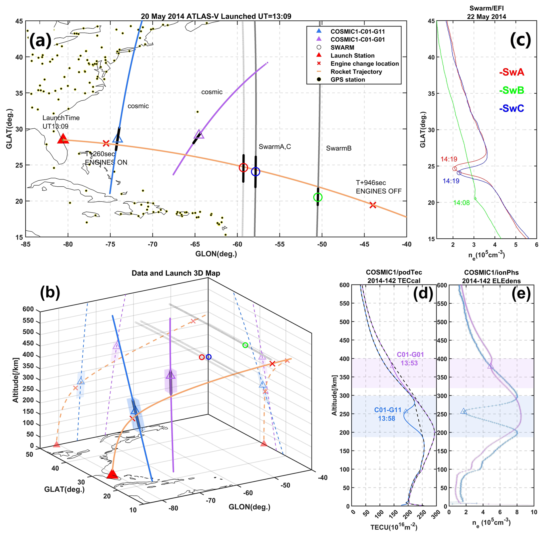
Figure 1 Observation Data Distribution and Details. (a) Map of rocket launch data distribution: the orange line represents the rocket trajectory, the red triangle marks the launch site, the red “×” indicates the start and end points of the rocket's second-stage engine working; The projection of COSMIC observation location points are shown as blue and purple lines, with triangular markers indicating detected depletion locations. The red/green/blue symbols represent REDs center observed by Swarm-Alpha/Bravo/Charlie, the gray dashed lines their trajectories. (b) 3D rocket trajectory (geographic projections) with COSMIC puncture-line shading indicating depletion extents. (c) Electron density measurements from Swarm satellites, with UT time at each marked point. (d) COSMIC TEC profile, with shaded REDs region and corresponding UT time. (e) COSMIC electron density profile.

2.2 Data and methods

The Constellation Observing System for Meteorology, Ionosphere, and Climate (COSMIC) radio occultation data have been widely applied in studies of the atmosphere, climate, and ionosphere. The gridded data products derived from COSMIC occultation observations have been used in rocket-induced depletion (RED) studies (Park et al., 2022). Moreover, COSMIC occultation data are frequently employed to monitor and investigate ionospheric disturbances caused by special events such as earthquakes, tsunamis, and sporadic Es layers (Astafyeva et al., 2011; Arras and Wickert, 2017; Yan et al., 2018, 2020, 2022; Qiu et al., 2021). A detailed assessment of the feasibility and reliability of COSMIC radio occultation data can be found in Lei et al. (2007) for COSMIC-1 and in Lin et al. (2020) for COSMIC-2. In this study, we utilize the electron density and total electron content (TEC) data derived from COSMIC-1 occultations (Level 1b, 1/60 Hz; product identifiers: ionPhs_repro and podTec_repro) to identify electron density depletions induced by rocket exhausts and to determine their corresponding altitude information. The COSMIC-1 datasets are provided by the COSMIC Data Analysis and Archive Center (CDAAC) and are available at https://data.cosmic.ucar.edu/gnss-ro/ (last access: 1 April 2026).

To investigate the horizontal spatial distribution of the REDs, we used data from ground-based GNSS receivers. The vertical total electron content (TEC) was calculated following the method described by Yan et al. (2017). The GNSS receiver data were obtained from the SOPAC & CSRC database service website (http://garner.ucsd.edu/, last access: 1 April 2026). The ionospheric total electron content (TEC), defined as the total number of electrons integrated along the signal path I (unit: m⁻² × 10¹⁶ m⁻² = 1 TECU), was derived from dual-frequency GPS carrier phase ($L_{\mathrm{1}}/L_{\mathrm{2}}$) and pseudorange ($P_{\mathrm{1}}/P_{\mathrm{2}}$) measurements. The computation was based on the ionospheric refraction model proposed by Klobuchar (1991):

$$\begin{array}{}\text{(1)}& {\displaystyle }& {\displaystyle }{\mathrm{STEC}}_{\mathrm{L}}=\left[\left({\displaystyle \frac{f_{\mathrm{2}}^{\mathrm{2}}}{f_{\mathrm{1}}^{\mathrm{2}}-f_{\mathrm{2}}^{\mathrm{2}}}}\right){\displaystyle \frac{f_{\mathrm{1}}^{\mathrm{2}}}{\mathrm{40.3}}}\right]\left(L_{\mathrm{1}}{\mathit{\lambda }}_{\mathrm{1}}-L_{\mathrm{2}}{\mathit{\lambda }}_{\mathrm{2}}\right)\text{(2)}& {\displaystyle }& {\displaystyle }{\mathrm{STEC}}_{\mathrm{P}}=\left[\left({\displaystyle \frac{f_{\mathrm{2}}^{\mathrm{2}}}{f_{\mathrm{1}}^{\mathrm{2}}-f_{\mathrm{2}}^{\mathrm{2}}}}\right){\displaystyle \frac{f_{\mathrm{1}}^{\mathrm{2}}}{\mathrm{40.3}}}\right]\left(L_{\mathrm{1}}{\mathit{\lambda }}_{\mathrm{1}}-L_{\mathrm{2}}{\mathit{\lambda }}_{\mathrm{2}}\right)\text{(3)}& {\displaystyle }& {\displaystyle }\mathrm{STEC}={\mathrm{STEC}}_{\mathrm{P}}+\sqrt{\sum _{i=\mathrm{1}}^N{\left({\mathrm{STEC}}_{\mathrm{L}}-{\mathrm{STEC}}_{\mathrm{P}}\right)}^{\mathrm{2}}/N}\end{array}$$

where f₁ and f₂ are GPS signal frequencies at 1.57542 and 1.2276 GHz, respectively; λ₁ and λ₂ are the corresponding wavelengths; N is the number of measurements sampled during a satellite pass.

The calculated STEC was projected onto the sub-ionospheric point (SIP) on the Earth's surface using an ionospheric single-layer model. The vertical TEC (VTEC) can then be derived from the following equation (Jin et al., 2008):

$$\begin{array}{}\text{(4)}& \mathrm{VTEC}=\left(\mathrm{STEC}-B^{\mathrm{S}}-B_{\mathrm{R}}\right)\times \sqrt{\mathrm{1}-{\left({\displaystyle \frac{r_{\mathrm{e}}\cos \mathit{\theta }}{r_{\mathrm{e}}+h_{\mathrm{ion}}}}\right)}^{\mathrm{2}}}\end{array}$$

where B^S and B_R are the instrumental biases related to GPS satellites and receivers, respectively; r_e=6371 km is the mean radius of the Earth; h is the elevation angle of a GPS satellite; h_ion is the height of the single ionosphere model, 350 km in this study. Below we use the TEC in place of VTEC for convenience.

Based on the TEC data, the identification method proposed by Pradipta et al. (2015) for ionospheric plasma bubbles was adopted and optimized using a third-order polynomial fitting to capture the specific characteristics of REDs. This approach allows for a more accurate extraction of the absolute vertical TEC depletion values and provides a clearer representation of the horizontal distribution features of the REDs.

The Swarm constellation, comprising three satellites at orbital altitudes of 450–550 km, is equipped with Langmuir probes to measure electron density, enabling the observation of REDs. Park et al. (2016) first reported Swarm observations of REDs, with detailed descriptions of the instruments and data available in their study. The Swarm data are sourced from the European Space Agency (ESA): https://swarm-diss.eo.esa.int/#swarm (last access: 1 April 2026).

2.3 Simulation of RED

The formation of ionospheric electron density depletion is closely linked to the diffusion patterns and chemical reactions of rocket-exhaust (e.g. Bowden et al., 2020; Zhao et al., 2024). Previous studies have shown that releasing around 4 kg of water vapor at 210 km altitude can cause significant depletions, with the affected area expanding at higher altitudes (e.g. Hu et al., 2010, 2011, 2013; Huang et al., 2011). Factors like release trajectory, exhaust flow rate, source speed, geomagnetic declination, and background winds further influence depletion patterns (e.g. Zhao et al., 2016; Feng et al., 2021; Gao et al., 2017). In this study, we also incorporate the effects of daytime electric fields and photoionization to improve simulation accuracy.

Rocket launches consume up to 79 % of their fuel below 80 km altitude, representing the predominant portion of total fuel consumption (Barker et al., 2024). The ATLAS-V first-stage core carries 284 t of fuel, with boosters attached to it, while the second stage carries 20.83 t. The first stage alone accounts for over 93 % of the total fuel load. As it releases most exhaust in the lower atmosphere and below the ionospheric D-region, the influence of first-stage exhaust on the REDs analyzed in this study is negligible. We selected the second stage ignition (∼260 s after launch at ∼200 km altitude) as the starting point of a 684 s exhaust release. The second-stage engine thrust for the ATLAS-V is approximately 22 890 lbs (equivalent to 10 382.73 kg), with a specific impulse (I_sp) of 449.7 s. Based on the standard formula relating thrust, specific impulse, and exhaust flow rate (Feng et al., 2021):

$$\begin{array}{}\text{(5)}& I_{\mathrm{sp}}={\displaystyle \frac{F}{g_{\mathrm{0}}\dot{m}}}\end{array}$$

where I_sp is the specific impulse, F represents thrust, and $\dot{m}$ is the released flow rate. The mass flow rate is calculated to be approximately 23.08 kg s⁻¹. Assuming a 5.5:1 oxidizer-to-fuel ratio, the mass fraction of water vapor in the exhaust is estimated to be ∼95 %, and hydrogen ∼5 % (Mendillo et al., 1975).

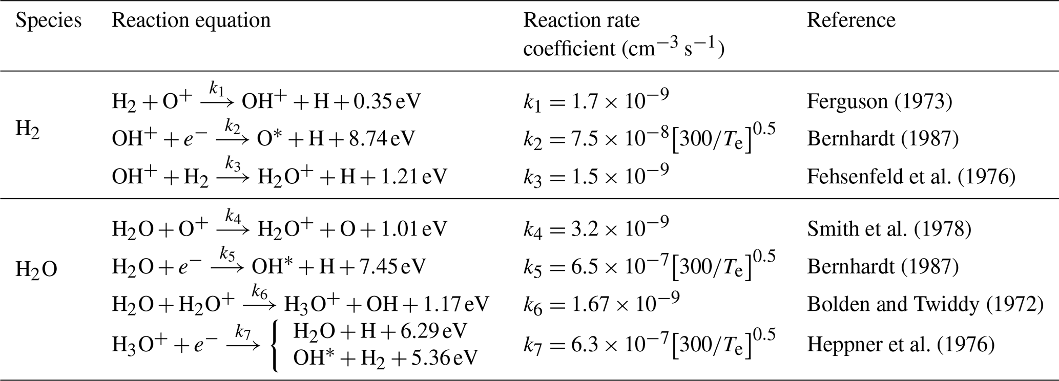
Table 1 The main chemical equations involved in the simulation release.

The diffusion equation proposed by Bernhardt (1976) for neutral material release calculates the molecular density of a point source as:

$$\begin{array}{}\text{(6)}& \begin{array}{rl}n(x,y,z,t)& ={\displaystyle \frac{N_{\mathrm{0}}}{{\left(\mathrm{4}\mathit{\pi }{D}_{\mathrm{0}}t\right)}^{\mathrm{1.5}}}}\exp \left\{-\left(z-z_{\mathrm{0}}\right)\left({\displaystyle \frac{\mathrm{3}}{\mathrm{4}{H}_{\mathrm{a}}}}+{\displaystyle \frac{\mathrm{1}}{\mathrm{2}{H}_{\mathrm{r}}}}\right)\right.\\ & -{\displaystyle \frac{H_{\mathrm{a}}^{\mathrm{2}}{\left\{-\left(z-z_{\mathrm{0}}\right)/\left(\mathrm{2}{H}_{\mathrm{a}}\right)\right\}}^{\mathrm{2}}}{D_{\mathrm{0}}t}}-\mathit{\beta }t\\ & -{\displaystyle \frac{\left(x^{\mathrm{2}}+y^{\mathrm{2}}\right)\exp \left[-\left(z-z_{\mathrm{0}}\right)/\left(\mathrm{2}{H}_{\mathrm{a}}\right)\right]}{\mathrm{4}{D}_{\mathrm{0}}t}}\\ & \left.-{\left({\displaystyle \frac{\mathrm{1}}{H_{\mathrm{a}}}}-{\displaystyle \frac{\mathrm{1}}{H_{\mathrm{r}}}}\right)}^{\mathrm{2}}{\displaystyle \frac{D_{\mathrm{0}}t\exp \left[\left(z-z_{\mathrm{0}}\right)/\left(\mathrm{2}{H}_{\mathrm{a}}\right)\right]}{\mathrm{4}}}\right\}.\end{array}\end{array}$$

D₀ is the diffusion coefficient follows Mendillo et al. (1993); H_a and H_r (H = kT mg⁻¹) are the atmospheric scale heights for air and the release substance, respectively; z₀ is the release altitude; where β is a loss coefficient that includes chemical reactions and photoionization.

The diffusion coefficient (D₀) is a key parameter controlling the temporal evolution and spatial distribution of neutral species. It depends on the molecular number density and ambient temperature of the background atmosphere at the release altitude. In the ionospheric region, the dominant neutral constituents are atomic oxygen (O), molecular nitrogen (N₂), and molecular oxygen (O₂). The diffusion coefficients of the released species, such as H₂O and H₂, are calculated following the method of Mendillo et al. (1993), and can be expressed in a simplified form as:

$$\begin{array}{}\text{(7)}& {\displaystyle }\begin{array}{rl}{D}_{{\mathrm{H}}_{\mathrm{2}}\mathrm{O}}& =\left[{\displaystyle \frac{n_{\mathrm{O}}}{\mathrm{8.46}\times {\mathrm{10}}^{\mathrm{17}}{T}_{\mathrm{n}}^{\mathrm{0.5}}}}+{\displaystyle \frac{n_{{\mathrm{N}}_{\mathrm{2}}}}{\mathrm{2.04}\times {\mathrm{10}}^{\mathrm{17}}{T}_{\mathrm{n}}^{\mathrm{0.632}}}}\right.\\ & {\left.+{\displaystyle \frac{n_{{\mathrm{O}}_{\mathrm{2}}}}{\mathrm{2.02}\times {\mathrm{10}}^{\mathrm{17}}{T}_{\mathrm{n}}^{\mathrm{0.632}}}}\right]}^{-\mathrm{1}}{\mathrm{cm}}^{\mathrm{2}}{\mathrm{s}}^{-\mathrm{1}}\end{array}\text{(8)}& {\displaystyle }\begin{array}{rl}{D}_{{\mathrm{H}}_{\mathrm{2}}}& =\left[{\displaystyle \frac{n_{\mathrm{O}}}{\mathrm{2.97}\times {\mathrm{10}}^{\mathrm{18}}{T}_{\mathrm{n}}^{\mathrm{0.5}}}}+{\displaystyle \frac{n_{{\mathrm{N}}_{\mathrm{2}}}}{\mathrm{2.8}\times {\mathrm{10}}^{\mathrm{17}}{T}_{\mathrm{n}}^{\mathrm{0.740}}}}\right.\\ & {\left.+{\displaystyle \frac{n_{{\mathrm{O}}_{\mathrm{2}}}}{\mathrm{3.06}\times {\mathrm{10}}^{\mathrm{17}}{T}_{\mathrm{n}}^{\mathrm{0.732}}}}\right]}^{-\mathrm{1}}{\mathrm{cm}}^{\mathrm{2}}{\mathrm{s}}^{-\mathrm{1}}\end{array}\end{array}$$

where n_O, $n_{{\mathrm{N}}_{\mathrm{2}}}$, $n_{{\mathrm{O}}_{\mathrm{2}}}$ denotes the number densities of O, N₂, and O₂, and T_n is the neutral atmospheric temperature.

By moving point sources along the rocket trajectory, we simulate continuous rocket exhaust diffusion (e.g. Zhao et al., 2016; Feng et al., 2021). H₂O and H₂ released into the ionosphere mainly participates in the following reactions as Table 1, to deplete ionospheric electrons:

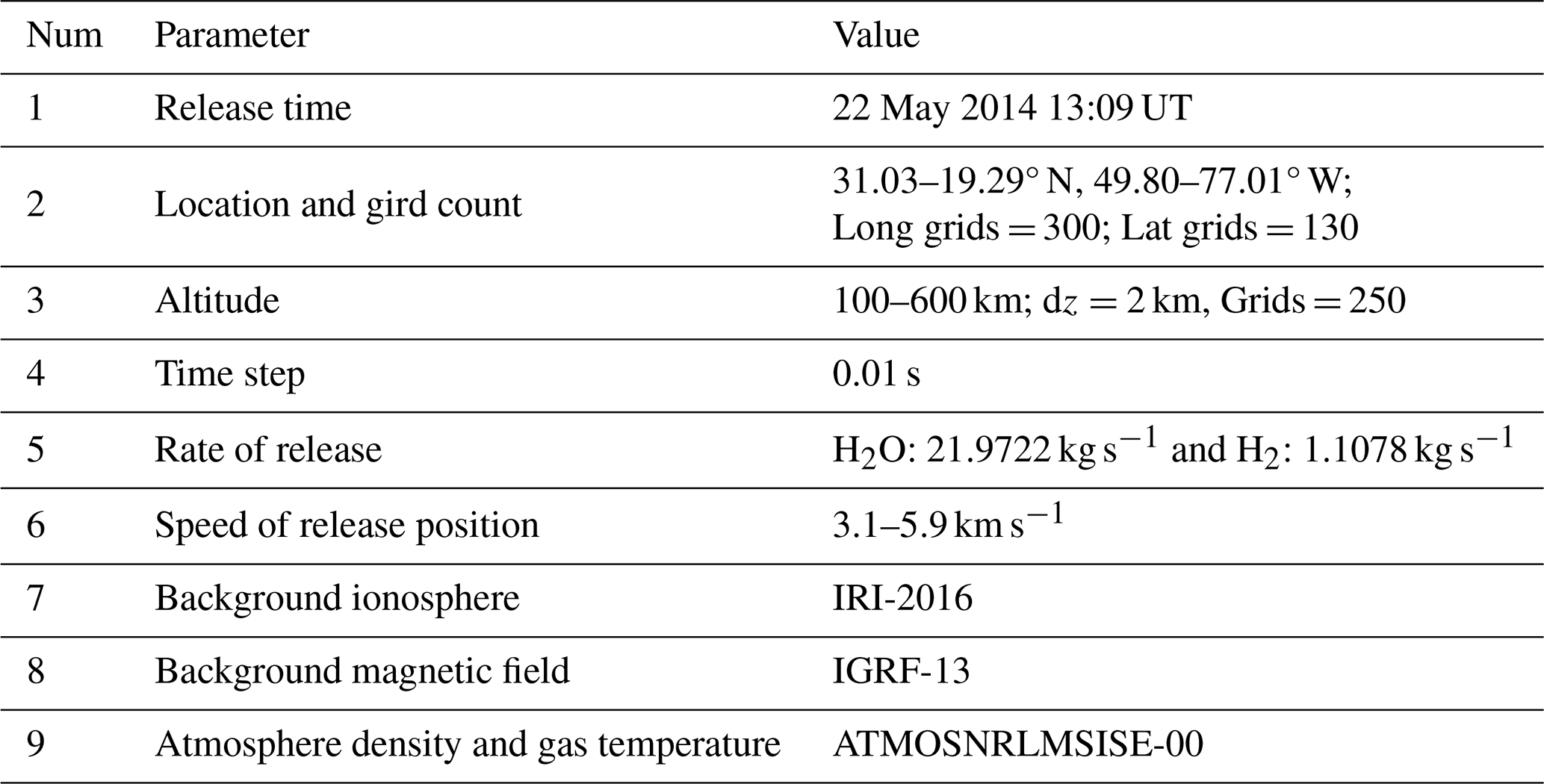
Table 2 Parameter settings and background model for numerical simulation.

k₁–k₇ represent chemical reaction rates; T_e is electron temperature. Based on the methodology of Mendillo et al. (1993), the electron density variation per time step Δt resulting from chemical reactions of the type $A+B\stackrel{k_i}{⟶}C+D$ (where k_i represents the reaction rate coefficient) is calculated. The expression for the concentration changes of reactants and products involved in the reaction per time step Δt is given as:

$$\begin{array}{}\text{(9)}& \mathrm{\Delta }{n}_i=k_i\cdot n_A\cdot n_B\cdot \mathrm{\Delta }t.\end{array}$$

Neutral release disrupts ionospheric equilibrium, inducing plasma diffusion. Assuming the dominant influence of the geomagnetic field, plasma diffusion is primarily motion along magnetic field lines, with its continuity equation expressed as:

$$\begin{array}{}\text{(10)}& {\displaystyle \frac{\partial n_{\mathrm{p}}}{\partial t}}=-\mathrm{\nabla }\cdot \left(n_{\mathrm{p}}{\mathit{v}}_{\perp }+n_{\mathrm{p}}{\mathit{v}}_{//}\right)+P_{\mathrm{p}}-L_{\mathrm{p}}\end{array}$$

where n_p is charged particle density distribution, P_p and L_p are particle production and loss terms; ${\mathit{v}}_{//}$ and v_⊥ are the velocity vector parallel and perpendicular to the magnetic field. Geomagnetic inclination (I) and declination (φ) define the field direction, with s along the magnetic field line. Plasma diffusion speed along the magnetic field is expressed as:

$$\begin{array}{}\text{(11)}& {\mathit{v}}_{//}=-D_{\mathrm{p}}\left[{\displaystyle \frac{\partial \ln \left(n_{\mathrm{p}}{T}_{\mathrm{p}}\right)}{\partial s}}+{\displaystyle \frac{\sin I}{H_{\mathrm{p}}}}\right]+v_{\mathrm{D}}\end{array}$$

$$\begin{array}{}\text{(12)}& {\mathit{v}}_{\perp }={\displaystyle \frac{\mathit{E}\times \mathit{B}}{B^{\mathrm{2}}}}+{\displaystyle \frac{m}{q}}{\displaystyle \frac{\mathit{g}\times \mathit{B}}{B^{\mathrm{2}}}}.\end{array}$$

D_p is the plasma diffusion coefficient, $D_{\mathrm{p}}=(\mathrm{1}+T_{\mathrm{e}}/T_{\mathrm{i}})D_{\mathrm{i}}$, where D_i is the ion diffusion coefficient; T_p is plasma temperature, $T_{\mathrm{p}}=(T_{\mathrm{i}}+T_{\mathrm{e}})/$2; H_p is the plasma scale height, $H_{\mathrm{p}}=k(T_{\mathrm{e}}+T_{\mathrm{i}})/m_{i}g$; v_D represents external drift velocity; g is gravitational acceleration, and q is the ion charge. The E×B drift velocity term for v_⊥ is provided by Anderson and Bernhardt (1978). Based on these equations, the plasma diffusion formula in a Cartesian coordinate system (x – east, y – north, z – up) is:

$$\begin{array}{}\text{(13)}& \begin{array}{rl}{\displaystyle \frac{\partial n_{\mathrm{p}}}{\partial t}}& ={\sin }^{\mathrm{2}}I\cdot \left[{\displaystyle \frac{\partial D_{\mathrm{p}}}{\partial z}}{\displaystyle \frac{\partial n_{\mathrm{p}}}{\partial z}}+{\displaystyle \frac{n_{\mathrm{p}}}{T_{\mathrm{p}}}}{\displaystyle \frac{\partial D_{\mathrm{p}}}{\partial z}}{\displaystyle \frac{\partial T_{\mathrm{p}}}{\partial z}}+{\displaystyle \frac{n_{\mathrm{p}}}{H_{\mathrm{p}}}}{\displaystyle \frac{\partial D_{\mathrm{p}}}{\partial z}}\right.\\ & +{\displaystyle \frac{D_{\mathrm{p}}}{T_{\mathrm{p}}}}{\displaystyle \frac{\partial n_{\mathrm{p}}}{\partial z}}{\displaystyle \frac{\partial T_{\mathrm{p}}}{\partial z}}+{\displaystyle \frac{D_{\mathrm{p}}}{H_{\mathrm{p}}}}{\displaystyle \frac{\partial n_{\mathrm{p}}}{\partial z}}+D_{\mathrm{p}}{n}_{\mathrm{p}}{\displaystyle \frac{\partial \left(\mathrm{1}/H_{\mathrm{p}}\right)}{\partial z}}\\ & \left.-{\displaystyle \frac{D_{\mathrm{p}}{n}_{\mathrm{p}}}{T_{\mathrm{p}}^{\mathrm{2}}}}{\left({\displaystyle \frac{\partial T_{\mathrm{p}}}{\partial z}}\right)}^{\mathrm{2}}+{\displaystyle \frac{D_{\mathrm{p}}{n}_{\mathrm{p}}}{T_{\mathrm{p}}}}{\displaystyle \frac{{\partial }^{\mathrm{2}}T}{\partial z^{\mathrm{2}}}}\right]+{\sin }^{\mathrm{2}}I\cdot D_{\mathrm{p}}{\displaystyle \frac{{\partial }^{\mathrm{2}}{n}_{\mathrm{p}}}{\partial z^{\mathrm{2}}}}\\ & -v_{\mathrm{D}}\sin I{\displaystyle \frac{\partial n_{\mathrm{p}}}{\partial z}}+{\cos }^{\mathrm{2}}I\sin \mathit{\varphi }\cdot D_{\mathrm{p}}{\displaystyle \frac{{\partial }^{\mathrm{2}}{n}_{\mathrm{p}}}{\partial x^{\mathrm{2}}}}\\ & +\sin I\sin \mathit{\varphi }{\displaystyle \frac{D_{\mathrm{p}}}{H_{\mathrm{p}}}}{\displaystyle \frac{\partial n_{\mathrm{p}}}{\partial x}}-v_{\mathrm{D}}\cos I\sin \mathit{\varphi }{\displaystyle \frac{\partial n_{\mathrm{p}}}{\partial x}}\\ & +{\cos }^{\mathrm{2}}I\cos \mathit{\varphi }\cdot D_{\mathrm{p}}{\displaystyle \frac{{\partial }^{\mathrm{2}}{n}_{\mathrm{p}}}{\partial y^{\mathrm{2}}}}+\sin I\cos I{\displaystyle \frac{D_{\mathrm{p}}}{H_{\mathrm{p}}}}{\displaystyle \frac{\partial n_{\mathrm{p}}}{\partial y}}\\ & -v_{\mathrm{D}}\cos I\cos \mathit{\varphi }{\displaystyle \frac{\partial n_{\mathrm{p}}}{\partial y}}+P-L+{\mathit{v}}_{\perp }\mathrm{\nabla }{n}_{\mathrm{p}}.\end{array}\end{array}$$

The numerical model, built upon the above theoretical framework, simulates the launch scenario of Event-1 using a central finite-difference scheme. Table 2 summarizes the background models and simulation parameters.

3 Result and discussion

3.1 Observation

Figure 1a and b presents the rocket trajectory and observed depletion locations for Event-1. Figure 1d and e presents the vertical profiles of TEC and electron density from COSMIC-1 satellite C01 paired with navigation satellites G01 and G11, labeled as C01–G11 and C01–G01. Both radio occultation events occurred within 10 min, with triangular markers indicating the depletion centers and corresponding UT timestamps. For the C01–G11 at UT 13:58, about 40 min after the ATLAS-V rocket's second-stage ignition, depletion was observed between 197–300 km altitude, showing a maximum TEC drop of ∼50 TECU and an electron density reduction of ∼75 % at 250 km. The C01–G01 at 13:53 UT recorded depletion between 310–400 km, with an electron density ∼15 % reduction at 375 km. The lower boundary, estimated using Pradipta et al. (2015), was between 250–320 km for C01–G01. Because the vertical profiles of occultation data not only record altitude information but also extend along the north–south direction across several thousand kilometers, an occultation ray may intersect the horizontal extent of the REDs region. Therefore, the upper and lower boundaries observed in occultation profiles do not necessarily represent the true vertical limits of the REDs. Furthermore, due to the asymmetric vertical distribution of REDs, the upper and lower boundaries of the depletion vertical scale derived from COSMIC radio occultation observations are subject to certain errors. Additionally, low-Earth-orbit occultation measurements are influenced by atmospheric refraction, leading to altitude-dependent spatial uncertainties. At the hmF2 altitude, the average deviation is approximately 33 km (Xu et al., 2010). Consequently, the altitude distribution of REDs derived from COSMIC occultation data contains uncertainties on small spatial scales.

As supporting evidence, these REDs were previously reported by Park et al. (2015, 2016) using Swarm in situ measurements, which are also retrieved in this study (Fig. 1c). Swarm-Alpha/Bravo/Charlie are marked in different colors, with times of minimum depletion labeled. The Swarm observations occurred around 14:00 UT. Altitudes are shown in Fig. 1c, where Swarm A and C orbited at 469.9 km, and Swarm B at 518.5 km. The north-south REDs lengths recorded by Swarm A, C, and B were 419, 491, and 277 km, respectively, with maximum electron density reductions of about 45 %, 39 %, and 5 %. The horizontal distribution of REDs measured by Swarm closely followed the rocket's projected ground track.

Figure 2 presents the REDs characteristics extracted from ground-based GNSS TEC data for Event-1 and Event-2. Figure 2a shows the GNSS data distribution for Event-1, Fig. 2b shows the corresponding time series of the identified REDs in differential TEC (DTEC). The vertical axis is arranged according to the closest distance from the observation points to the rocket trajectory, indicating the observed REDs' distance from the rocket path. Due to the offshore launch and limited temporal coverage, most GNSS data failed to capture the REDs. Some ionospheric piercing points (IPPs) near the second-stage ignition site and occultation region did not capture RED signatures because they arrived 2–3 h after launch, by which time the RED had drifted northward out of the area. To improve visualization, the data points without detected REDs signatures are semi-hidden. Figure 2a also shows the horizontal TEC distribution map, where red small triangles indicate the recording position for each data curve at the launch time, and black arrows mark the time sequence of data measurement. For Event-1, the GNSS effective observation data is sparse; the maximum depletion amplitude observed occurred approximately 1.5 h after the launch, with a magnitude of about 9 TECU (1 TECU = 10¹⁶ electrons square meter) at a distance of ∼200 km from the rocket trajectory, located near the C01–G01.

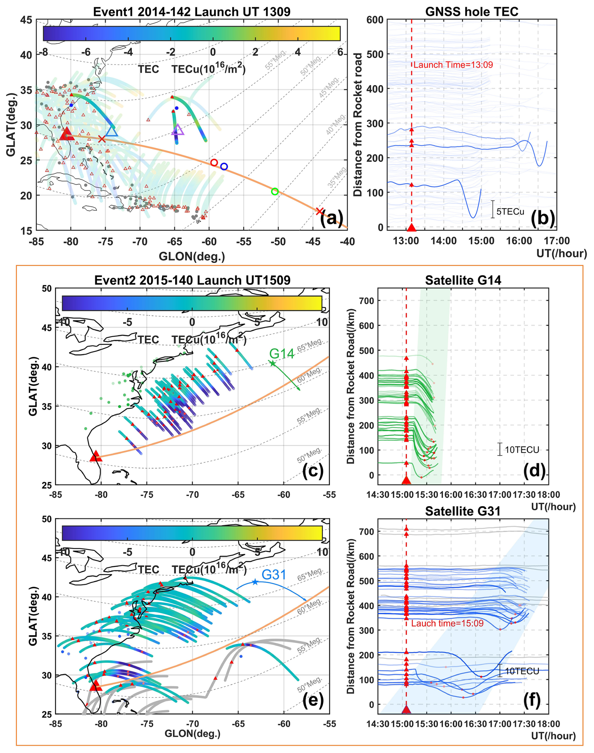
Figure 2 GNSS TEC data for Event-1 and Event-2. (a, c, e) TEC IPPs maps: the large red triangle marks the launch site, the orange line shows the rocket trajectory, small red triangles indicate IPPs at launch time, black arrows show their movement, and color represents depletion magnitude. (b, d, f) Time series of extracted TEC depletion; red dashed lines mark launch time. (a, b) Event-1: (a) IPPs distribution; (b) depletion time series. (c–f) Event-2: (c, e) IPPs from G14 and G31; (d, f) corresponding depletion time series.

Due to sparse GNSS coverage along Event-1's rocket trajectory, accurate horizontal depletion scales could not be determined. Therefore, Event-2 serves as a reference, given the identical rocket model, similar launch trajectory, and matching local time. Figure 2c–f depicts the horizontal TEC distribution and time-series depletion signals from Event-2. Figure 2c and e shows the IPPs for TEC observed at 300 km by the G14 and G31. The corresponding time-series signals in Fig. 2d and f are arranged by the shortest distance to the rocket trajectory, similar to Fig. 2b. For Event-2, the REDs extended up to ∼500 km across the trajectory and exceeded 2000 km in length, with a maximum TEC reduction of approximately 20 TECU, lasting over 2 h.

3.2 Simulation

Figure 3 shows the simulation result of H₂O release and electron density depletion for Event-1. Figure 3a–d illustrates the evolution of H₂O molecular density along the rocket flight path. Water vapor diffuses rapidly within the first few minutes, spreading laterally along the trajectory, with a vertical range of around 100 km. Molecular density decreases gradually as diffusion slows, reaching maximum spread at about 25 min, before gravitational settling pulls it to lower altitudes, ceasing its contribution to depletion consistent with Zhao et al. (2024). Figure 3e–h shows electron density changes during water release. Depletion forms within 1–2 min, spreading for about 20 min. And depletion mainly extends laterally along the trajectory, reaching 180 km upwards and 50 km downwards. Recovery follows, with faster recovery at lower altitudes due to higher background density, showing an upward drift pattern consistent with Zhao et al. (2024). At 50 min, the depletion reaches a thickness of 150–300 and 200–500 km in vertical range. We have included multiple detailed depletion evolution videos in the video materials (Videos S1–S3 in the Supplement), which visualize the simulated 3D spatiotemporal evolution processes.

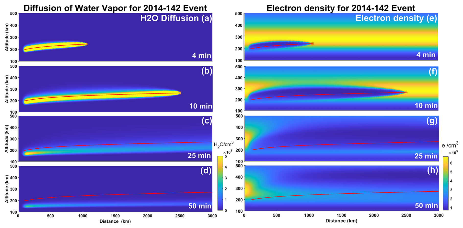
Figure 3 Simulation molecular density distribution of H₂O and electrons. (a–d) H₂O molecular density distribution along the rocket trajectory (height vs. flight distance). (e–h) Electron density distributions along the rocket trajectory. (a–h) Time (lower-right corners): minutes after second-stage ignition; red line is rocket trajectory; red star is current release position.

In the simulation results, Fig. 4a shown the distribution of the vertical TEC variation. The simulated TEC variation intensity is approximately 10 TECU, and the simulated depletion is primarily distributed along the release trajectory, with a horizontal width perpendicular to the trajectory of about 500 km. Figure 4b–d presents a comparison of electron density between the Swarm A, Swarm C, and Swarm B satellites and the simulations. The simulation results show that at the location corresponding to Swarm A, the electron density reduction amplitude is 1.6×10⁶ cm⁻³ (with an observed reduction of 1.9×10⁶ cm⁻³), and the background change rates are 65.6 % and 65.7 %, respectively, significantly higher than the depletion amplitudes of 45 % and 39 % observed by Swarm A and Swarm C. The background electron density observed by the satellites is significantly higher than that output by the IRI model; this discrepancy affects the chemical reaction efficiency and extent, representing a primary reason for the differences between the simulation and observations. Figure 4e and f shows a comparison between the integral of electron density along the simulated COSMIC radio occultation ray path and the podTEC from occultation observations. The simulated TEC variation is about 40 TECU, and the depletion altitude ranges are 120–305 and 220–450 km, respectively, which are broader than those observed in the two occultation events. The background TEC is significantly lower than the observed values, primarily due to the combined effects of the occultation ray path geometry and errors in the background electron density from the IRI model.

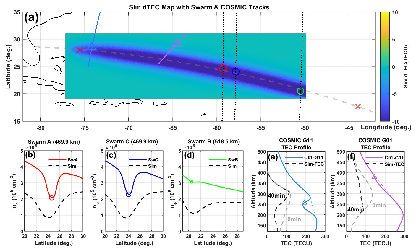
Figure 4 Comparison of the simulated dTEC calculation at the 40th minute with observational data. (a) The variation in the vertical integral of the simulated electron density, dTEC; (b–d) comparison of electron density between Swarm satellites and simulations; (e, f) comparison of the integral of electron density along the simulated COSMIC radio occultation ray path with the podTEC from occultation observations.

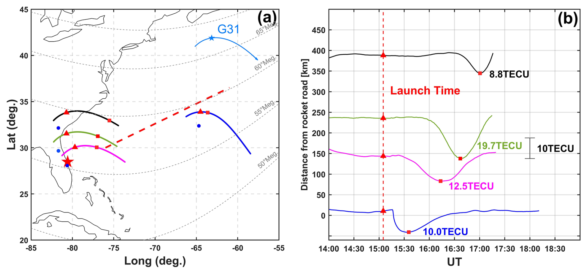
Figure 5 TEC signals of the depletion observed within the REDs at several different time intervals. (a) Map of piercing points: red triangles indicate the positions of piercing points at the rocket launch time; small red squares mark the positions where the maximum TEC values of the REDs were recorded; blue circles represent GPS stations; red pentagrams indicate the rocket launch site; red dashed lines show the central line of the REDs. (b) Extracted TEC profiles of the depletion: red dashed lines denote the rocket launch time; red triangles and squares in different shades correspond to the elements shown in the left panel.

3.3 The evaluation of ELE hole

The ionospheric piercing points (IPPs) for TEC data derived from ground-based GPS receivers shift over time, providing temporal sequences of REDs observations at different intervals. As shown in Fig. 5, for the IPPs closest to the rocket trajectory (blue line), the TEC begins to drop approximately 10 min after launch – this 10 min delay corresponds to the time required for the rocket to reach the vicinity of this IPPs. The decrease occurs rapidly within 3–5 min, followed by a slower decline. Since this location (blue line) is at the edge of the main REDs, the maximum depletion amplitude observed here is about 10 TECU, which is weaker than the values recorded later by IPPs that pass directly through the depletion (green and pink lines). For IPPs entering the REDs more than 20 min after launch, the TEC variations exhibit smoother curves. The maximum depletion amplitude for this entire event is recorded around 90 min post-launch. Furthermore, as indicated in Fig. 2, most TEC variations observed after 90 min are collectively weaker than the maximum amplitude captured by the green line. This suggests that the REDs subsequently entered a diffusion-driven recovery stage after 90 min, gradually returning to background levels.

The horizontal evolution of REDs in Event-1 is consistent with Event-2 (same rocket type) and prior cases (e.g. Mendillo et al.,2008), where depletions exceeded >2000 km in length and ∼500 km in width from the same launch site. The REDs evolution generally follows three stages: (i) formation within 5–7 min post-launch, with GNSS detecting rapid depletion; (ii) diffusion-driven growth over 25–30 min, expanding to 500–2200 km in length and 300–500 km in width; (iii) gradual recovery lasting over 50 min as density returns to background levels (e.g., Liu et al., 2018; Ozeki and Heki, 2010; Mendillo et al., 1975, 2008; Zhao et al., 2024). Vertical structures were observed by Wand and Mendillo (1984) between 200–500 km in a trajectory matching Event-1. Zhao et al. (2024) reported vertical ranges of ∼200–700 and ∼202–535 km from two rocket launches, classifying the vertical evolution into generation, diffusion, and recovery stages-consistent with horizontal evolution patterns.

Simulations show water vapor rapidly diffuses within 1–2 min, expand more slowly over ∼20 min, and eventually settle into lower atmospheric layers due to gravity; This aligns with previous studies (Hu et al., 2010, 2011; Gao et al., 2017; Zhao et al., 2024). The resulting REDs exhibit a vertically “top-wide, bottom-narrow” profile, consistent with Gao et al. (2017). This structure likely results from: (i) an exponential increase in diffusion coefficients with altitude, causing wider upper depletion; (ii) higher lower-altitude electron densities, promoting faster recovery and forming a narrower base. This matches Wand and Mendillo (1984) and aligns with COSMIC-1 occultation results, confirming the asymmetric vertical structure. GNSS data show TEC drops within 5–7 min of launch, lasting 1–2 min, and diffusing over 500 km in 15–25 min, consistent with simulations (Mendillo et al., 1975, 2008; Ozeki and Heki, 2010). Simulation began 260 s post-launch (second-stage ignition), showing rapid density drops within 2 min and peak diffusion at 20 min, closely matching GNSS observations. The simulated vertical range (200–500 km) matches Swarm A/C observations at 469 km and COSMIC-1 events, while Swarm B at 518 km, near the edge, recorded only ∼5 % variation, within simulation error margins.

3.4 The structure of ELE hole

Figure 1 shows COSMIC-1 occultation data and rocket data. Previous studies (Park et al., 2015, 2016) reported similar REDs lasting nearly 6 h using DMSP satellite data. For Event-1, GNSS data measured depletions ∼5 TECU even 3.5 h post-launch, indicating a prolonged lifetime. Both COSMIC-1 radio occultation events occurred within 50 min after the rocket launch, and the observed depletion regions were located within approximately 300 km of the rocket trajectory. This temporal and spatial proximity indicates that the observed ionospheric depletion was very likely caused by the rocket launch. For event C01–G11, the TEC depletion was about 50 TECU, with a corresponding electron density reduction exceeding 75 %; in contrast, event C01–G01 showed a weaker depletion, with a TEC decrease of about 13 TECU and an electron density reduction of less than 20 %. Previous studies have shown that the typical uncertainty of podTEC data derived from low Earth orbit radio occultation is about 2–3 TECU (Yue et al., 2011). In comparison, the depletion magnitudes observed in these two events are significantly larger than this uncertainty range, suggesting that the observed TEC depletions were mainly caused by rocket exhaust.

Swarm A and C, observing along the latter half of the trajectory, detected reductions around 40 %. Time differences between these four datasets were <30 min. The location of maximum depletion for C01–G11 was ∼110 km horizontally from the trajectory, while that for C01–G01 exceeded 300 km. This suggests that depletion strength depends on occultation proximity to the center. Similarly, Swarm B at 519 km altitude, near the depletion's edge, recorded ∼5 % variation, while Swarm A and C at 469 km, closer to the center, observed larger reductions. Multi-distance observations aided in positioning the 3D spatial structure of the REDs. However, the occultation tangent point reflects both vertical and horizontal variations, so it does not directly indicate depletion thickness. Since the occultation ray path is aligned east-west, matching the rocket trajectory, the associated uncertainty has minimal impact on the RED reconstruction. Therefore, the east-west systematic error in occultation observations can be neglected when estimating the 3D hollow-tube structure.

The observational period of the radio occultation data falls within the first 50 min after the rocket launch. Relative to the RED's total lifetime of nearly 6 h, this observational period places the RED in the early stage of its diffusion recovery phase, a period characterized by a considerable horizontal extent. According to previous studies summarized in Table 3, the horizontal width of the RED ranges from 150 to 520 km, depending on factors such as rocket type and launch trajectory. The RED generated by rockets of the same type performing the same orbital mission exhibit similar widths. Therefore, the REDs produced by Event-1 and Event-2 can be assumed to have comparable widths, approximately 500 km, which is used as the horizontal constraint for the three-dimensional RED structure.

Table 3 The Characteristics of RED by Rocket Launch Events in previous studies; TSLC is Taiyuan Satellite Launch Center of China (38.5° N, 111.6° E), KSC is Kennedy Space Center of USA (28.5° N, 80.7° W).

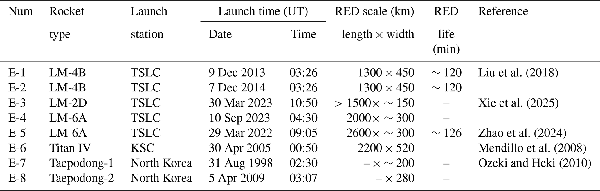
Figure 6 illustrates the simulated electron density distribution and the estimated spatial extent of the HIREs constrained by multi-dimensional observational data. The horizontal extent of the HIREs is constrained by GNSS TEC observations, while the vertical scale is jointly constrained by COSMIC and Swarm satellite altitude observations. The boundary of the vertical cross-section of the HIREs derived from numerical simulations is approximately elliptical. Based on the horizontal and vertical constraints, the ellipse-like boundaries are fitted to the COSMIC radio occultation and Swarm satellite observations. Polynomial fitting is then used to connect these boundaries, producing the red dashed tubular volume in Fig. 6, representing the observed HIREs extent. The three-dimensional simulated electron density distribution is displayed in cross-sectional view as six parallel colored panels in Fig. 6. By comparing the simulated HIREs with the fitted observational HIREs, the horizontal distance between the centers of the simulated and observed HIREs does not exceed 120 km, and for the COSMIC-1 C01–G11 occultation event, the distance between the observed and simulated HIREs centers is less than 30 km. The simulated HIREs is about 20 % wider than the observed electron depletion, likely due to discrepancies between the background parameters used in the simulation and the actual ionospheric conditions. Differences between IRI model outputs and real ionospheric TEC can exceed 20 % (He et al., 2023). As the HIREs extends over thousands of kilometers, it is subjected to varying background wind intensities and associated uncertainties at different locations. These variations, in turn, induce differential HIREs drift distances, resulting in positional discrepancies between the simulated HRIEs centerline and the observed 3D centerline.

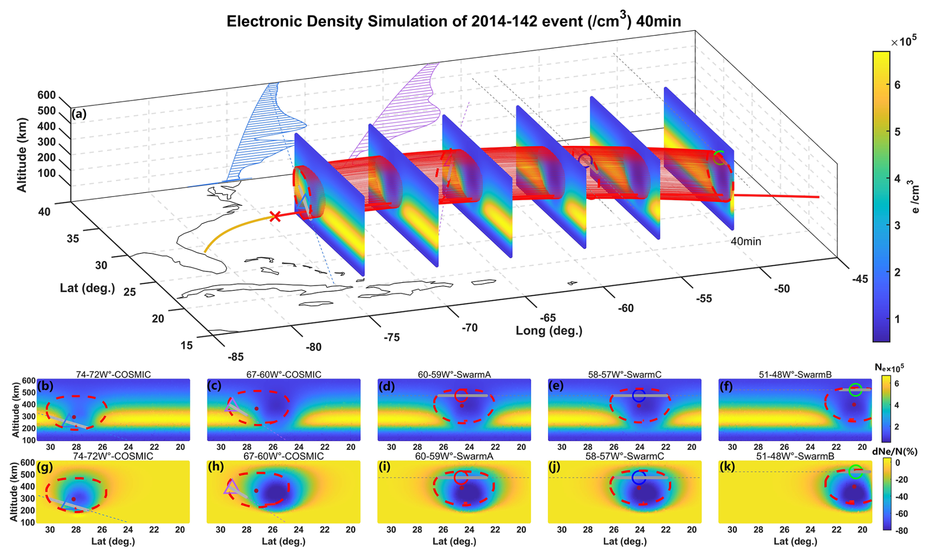
Figure 6 Simulated electron density distribution at 40 min and the range of HIREs. (a) The COSMIC-1 data tangent points (marked by dashed lines) with electron density profile projections on the 40° N vertical cross-section. The other marks are the same as Fig. 1. (b–f) The simulated and observed ranges in different latitudinal ranges; (g–k) the percentage change in electron density.

Combining simulation and observational results, the three-dimensional structure of the REDs is a “flattened hollow tube” with a wider top. The entire “flattened 3D hollow tube” envelops the launch trajectory, with the trajectory located closer to the lower side of the tube, resulting in an asymmetric vertical distribution of the RED along the trajectory. Simulation results indicate that the width and thickness of the “flattened 3D hollow tube” are primarily controlled by the amount and altitude of exhaust release and the background electron density distribution. The High-density area electron density layer is mainly located around 300 km in the ionospheric F₁ layer, where most chemical reactions of the rocket exhaust also occur, positioning the electron density depletion center near the F₁ layer. As atmospheric density decreases with altitude, the diffusion coefficient of the exhaust increases exponentially with height (Mendillo et al., 1975), causing upward diffusion to be faster and forming an upper-wide, lower-narrow, quasi-ellipsoidal shape. Exhaust released at lower altitudes can also diffuse upward toward the F₁ layer, producing stronger chemical reactions and generating larger amplitude electron density depletions at higher altitudes along the release trajectory.

By integrating the simulated vertical electron density, the equivalent vTEC as observed by ground-based GNSS can be obtained. In this study, equivalent observational integrals were also performed along the ray paths of two COSMIC radio occultation events, and the simulation results were compared with electron density measurements from the Swarm satellites, as shown in Fig. 4. The simulated vTEC depletion amplitude and spatial scale are generally consistent with ground-based GNSS observations; the discrepancies between the simulation and Swarm satellite observations primarily arise from the fact that the background electron density output by the IRI model is significantly lower than the observed values. In the chemical process of depletion formation, the recombination efficiency ($\mathrm{\Delta }{n}_i=k_i\cdot n_{\mathrm{A}}\cdot n_{\mathrm{A}}\mathrm{\Delta }t$) is related not only to the reaction rate constant k_i but also to the concentrations of the reacting species. A higher background electron density leads to a higher chemical recombination efficiency, resulting in a greater magnitude of electron density loss.The broader depletion range output from the simulation along the occultation ray path, compared to actual observations, is closely related to the diffusion coefficient of the released species. The diffusion coefficient is influenced by background atmospheric parameters, and the atmospheric component concentrations provided by the NRLMSISE model deviate from actual values, with a root mean square error of approximately 30 % and up to 100 % in extreme cases (Doornbos et al., 2008). This deviation affects the diffusion coefficient of the released species and further influences the concentration distribution of the diffusing species. Additionally, the IRI model exhibits errors in the background electron density and oxygen ion (O⁺) conditions, which further affect the efficiency and extent of the chemical reactions. The diffusion coefficient varies with altitude and local time, modulated by background atmospheric composition and temperature; lower atmospheric molecular concentrations or higher temperatures result in faster diffusion and broader distribution of the released species, leading to larger depletion scales (both width and thickness), but the accompanying concentration reduction results in a smaller depletion amplitude. Therefore, the primary mechanisms governing the characteristics of REDs can be attributed to the diffusion coefficient and background constituent concentrations, both of which are determined by the background conditions of the exhaust release.

4 Conclusion

This is the first study that utilizes COSMIC-1 occultation data to resolve the vertical structure of REDs, integrates Swarm and GNSS-TEC observations, and reconstructs its 3D hollowtube morphology. Observation-simulation comparisons validate model reliability and support a three-stage RED evolution framework: rapid formation, diffusion-driven growth, and recovery. The main conclusions are as follows:

1. Using COSMIC-1 radio occultation data, we for the first time observed the vertical distribution of REDs at different locations along the rocket trajectory. At a location 700 km from the launch site, the RED vertical extent is 197–300 km, while at another location 2600 km away, the observed vertical extent is 310–400 km.

2. By combining multi-dimensional observational data with three-dimensional numerical simulations, we reconstructed the three-dimensional tubular structure of the RED. Its vertical cross-section is an upper-wide, lower-narrow quasi-elliptical shape, with a vertical-to-horizontal thickness-to-width ratio of approximately 1:2. The horizontal width of the RED is mainly controlled by the amount and altitude of rocket exhaust release.

3. Based on observations and simulations, the evolution of rocket-exhausted ionospheric electron density depletion can be divided into three stages: rapid formation, diffusive growth, and diffusive recovery. During the first 3–5 min after exhaust release, the REDs undergoes rapid growth, with the fastest rate of electron density decrease. It then enters a 15–30 min diffusive growth stage, during which the REDs expands to its maximum spatial extent, with a vertical thickness ranging from 100–500 km and a horizontal width along the trajectory of 300–500 km. Finally, the REDs evolves into the diffusive recovery stage, lasting more than 50 min, longer than the preceding two stages. During this stage, the REDs slowly returns to background values while undergoing drift motions at different rates due to the influence of the magnetic field and background wind.

Due to the influence of factors such as local time, propellant characteristics, and orbital insertion, understanding of REDs' 3D evolution remains limited. Broader observational coverage and more diverse cases are needed to identify common patterns and better assess REDs' physical drivers and space weather impacts.