Temporal variability of NO_x emissions from power plants: a comparison of satellite- and inventory-based estimates

Satellite observations of nitrogen dioxide (NO₂) are a valuable tool for estimating nitrogen oxides (NO_x) emissions from point sources and can support carbon dioxide (CO₂) monitoring through emission ratios. We assess the capability of TROPOMI NO₂ measurements to quantify the seasonal and day-to-day temporal variability of NO_x emissions from eighteen power plants in Europe and the United States. Using the cross-sectional flux (CSF) method implemented in the ddeq Python library (version 1.1), we derive top-down emissions and compare two NO_x chemistry corrections approaches: a “local” method based on plume-resolving MicroHH simulations and a “global” method based on GEOS-Chem simulations. Annual top-down estimates using the local approach agree well with bottom-up estimates from the CORSO point source database, with a mean bias of 9 ± 20 % when aggregating point sources within 30 km. A regression analysis yields a slope of 1.05 ± 0.17 and a coefficient of determination of 0.68. The local correction yields emissions that are 58 ± 8 % higher than the global approach. Satellite-based estimates successfully captured seasonal and short-term variability in bottom-up emissions estimated from electricity generation in Europe and continuous emissions monitoring systems (CEMS) in the USA. However, limitations remain due to reduced winter coverage, emissions below the detection limit, overlapping plumes, and uncertainties in NO_x chemistry corrections especially for non-isolated facilities. Overall, our findings demonstrate that satellite NO₂ observations can effectively monitor the seasonality of NO_x emissions from power plants. Addressing remaining uncertainties will be essential for future emission monitoring systems and upcoming satellite missions targeting both NO₂ and CO₂.

1 Introduction

Anthropogenic emissions from power plants and industrial facilities are among the largest contributors to global emissions of air pollutants and greenhouse gases (GHGs), including carbon dioxide (CO₂) and nitrogen oxides (NO_x= NO₂+ NO) (Crippa et al., 2024). These emissions negatively impact air quality and drive climate change, significantly affecting human health, ecosystems, and global warming. Accurate and timely monitoring of these emissions is therefore essential for assessing progress toward air quality standards and climate mitigation targets. In particular, identifying and quantifying emission hot spots, i.e. cities, power plants and industrial facilities, is a key objective of the European CO₂ Monitoring and Verification Support (CO₂MVS) system. This system aims to support the European Union's climate policy by providing robust, independent emission estimates based on satellite observations (Janssens-Maenhout et al., 2020).

Emission quantification methods can broadly be categorized into bottom-up and top-down approaches. Bottom-up methods rely on direct measurements at emission sources using Continuous Emission Monitoring System networks (CEMS, e.g., Tang et al., 2020) or on estimates derived from activity data (e.g., fuel consumption) combined with emission factors (e.g., Guevara et al., 2024). While direct measurements based on CEMS can be accurate, they often have limited spatial and temporal coverage since only large point sources are mandated to be equipped with these monitoring systems. Estimates based on activity data are more scalable but typically involve larger uncertainties due to assumptions in emission factors and reporting practices (Super et al., 2020). Both approaches depend heavily on data provided by facility operators, which may be incomplete or inconsistent across regions. Top-down methods use atmospheric measurements such as remote sensing observations to infer point source emissions by linking observed trace gas concentrations to emission rates through inverse modeling (e.g., Kaminski et al., 2022; van der A et al., 2024) or mass balance techniques (e.g., Beirle et al., 2021; Kuhlmann et al., 2024; Hakkarainen et al., 2025; Leguijt et al., 2025; Varon et al., 2018). These methods leverage satellite instruments such as the Tropospheric Monitoring Instrument (TROPOMI) aboard Sentinel-5P, which provides high-resolution measurements of nitrogen dioxide (NO₂), carbon monoxide (CO), methane (CH₄), and other trace gases (Veefkind et al., 2012). By combining satellite observations with wind speed and atmospheric transport models, top-down approaches can offer independent, spatially and temporally resolved emission estimates. However, the accuracy of top-down approaches is limited by uncertainties in satellite observations and restrictions in spatial and temporal coverage (e.g., Santaren et al., 2025).

Given that CO₂MVS envisions assimilating individual emission estimates at the time of the satellite overpass, it is crucial to assess whether temporal variability in emissions can be captured using satellite instruments. This capability would enhance the system’s responsiveness to short-term changes in industrial activity, policy interventions, and episodic events such as maintenance shutdowns or fuel switching. In this context, satellite observations of NO₂ are of great interest because they are available daily from polar-orbiting satellites (e.g., TROPOMI) and hourly during the daytime from geostationary satellites (e.g., GEMS (Kim et al., 2020) and TEMPO (Zoogman et al., 2017)). Top-down NO_x emissions derived from these observations not only provide information on air quality but can also be combined with CO₂:NO_x emission ratios to estimate CO₂ emissions (e.g., Kuhlmann et al., 2021). NO_x emissions have been estimated, for example, from TROPOMI and TEMPO by Goldberg et al. (2019); Beirle et al. (2021, 2023); Lange et al. (2022); Sun et al. (2025). Although NO_x emission estimates derived from NO₂ observations are largely consistent across different quantification methods, comparisons with bottom-up CEMS measurements for power plants often reveal that top-down estimates systematically and substantially underestimate these reported emissions (Lange et al., 2022; Sun et al., 2025). Recent studies based on plume-resolving simulations with chemistry (Krol et al., 2024) suggest that the underestimation is caused by NO_x chemistry, where scaling factors used for NO₂-to-NO_x conversion and NO_x lifetime are too small and require larger values for strong point sources (Hakkarainen et al., 2024; Meier et al., 2024).

In this study, we focus on top-down estimates of NO_x emissions derived from TROPOMI NO₂ observations. We compare these satellite-based estimates with bottom-up emission inventories for Europe and the United States of America (USA), examining their consistency and discrepancies. Furthermore, we analyze the seasonal cycle of NO_x emissions and assess how well satellite data reflect known temporal patterns from bottom-up sources. Finally, we discuss the limitations of current top-down approaches and provide recommendations for methodological improvements.

2 Bottom-up emission estimates

This study analyzes emissions from a selection of large point sources: six power plants in Europe and twelve in the USA (Table 1). These facilities were chosen for their high emission rates (> 3 kt NO_x expressed as NO₂ a⁻¹) and the availability of high resolution temporal emission data derived from official sources (see paragraphs below). Annual bottom-up emission estimates were obtained from the CORSO point source database (Guevara et al., 2024, 2025), which provides annual emissions of CO₂, NO_x, CO, SO_x and CH₄ for the year 2021. The database includes emissions from power generation, iron and steel production and cement manufacturing per industrial facility at their exact geographical locations. For the European power plants, information on annual emissions is directly derived from the integrated Industrial Reporting Database provided by the European Environmental Agency (EEA, 2024), while for the U.S. power plants emissions are obtained from the Emissions and Generation Resource Integrated Database (eGRIDv2021;  US EPA, 2024). In addition to CORSO, we used the CAMS-GLOB-ANT (version 6.2) inventory (Soulie et al., 2024), which provides gridded anthropogenic emissions at global scale at 0.1° resolution for a total of 17 emission sectors, including power generation, manufacturing industry, road transport and residential and commercial combustion activities, among others. CAMS-GLOB-ANT is used to complement the point source data reported by CORSO and to provide context for regional background emissions.

Table 1 List of six power plants in Europe and twelve power plants in the USA analyzed in this study with emissions from CORSO point source database in kt NO_x expressed as NO₂ a⁻¹.

For U.S. power plants, daily NO_x emission reports were obtained from publicly available Clean Air Market Program Data (CAMPD) of the U.S. Environmental Protection Agency (EPA). These reports are based on CEMS installed at the facilities, providing high-frequency measurements of NO_x emissions. For European power plants, only annual emission totals are available because daily or hourly emission measurements are not publicly accessible. We therefore estimate hourly NO_x emissions by scaling annual totals using hourly actual electricity generation data from the ENTSO-E Transparency Platform (Hirth et al., 2018). This approach assumes a linear relationship between power output and NO_x emissions, which was also used by previous studies (Nassar et al., 2022).

According to EPA and EEA performance specifications, reported NO_x emissions are required to have a relative accuracy of 10 % (1σ) or better (US EPA, 2023; Brinkmann et al., 2018). We therefore assume that daily, monthly and annual reported NO_x emissions are accurate to within ±10 % of the annual totals. For European hourly and monthly estimates, additional uncertainties may arise from the assumed emission-power relationship and operational dynamics. However, for the purposes of this study, we consider these uncertainties to be encompassed within the 10 % range.

3 Top-down emission estimates

NO_x emissions of the European and U.S. power plants were estimated from NO₂ column images retrieved from the TROPOMI instrument aboard the Sentinel-5P satellite. TROPOMI is a nadir-viewing imaging spectrometer that measures back-scattered solar irradiance in the ultra-violet, visible, near-infrared and shortwave spectral range. It provides daily global coverage at a resolution of 3.5 km by 5 km at nadir, enabling the detection of localized NO₂ emission plumes of individual power plants. Tropospheric NO₂ vertical column densities (VCDs) are retrieved from the visible spectrum using differential optical absorption spectroscopy (DOAS) that provides slant column densities (SCDs). Following a troposphere-stratosphere separation, SCDs are converted to VCDs using air mass factors (AMFs) that correct for viewing geometry, surface reflectance, atmospheric scattering and the vertical distribution of NO₂ (Veefkind et al., 2012; van Geffen et al., 2022).

NO_x emissions were estimated using the cross-sectional flux (CSF) method, implemented in the open-source Python library for data-driven emission quantification (ddeq, Kuhlmann et al. (2024) for version 1.0). The ddeq library was originally developed for estimating CO₂ and NO_x emissions from synthetic satellite images of the Copernicus CO₂ Monitoring (CO₂M) mission (Kuhlmann et al., 2019, 2021). In the CoCO2 project, the library was extended with additional methods and was used for benchmarking different approaches for emission quantification of hot spots (Hakkarainen et al., 2024; Santaren et al., 2025). In this study, we use version 1.1 of the ddeq library, which includes several improvements over version 1.0. Notably, we have merged the two cross-sectional flux methods implemented in the ddeq library: the CSF (cross-sectional flux) implementation, which was originally developed by Kuhlmann et al. (2020) for CO₂M, and the light cross-sectional flux (LCSF) implementation, which was originally developed by Zheng et al. (2020) for OCO-2 and modified for CO₂M by Santaren et al. (2025). As a result, the CSF implementation can now identify the plume location based on the wind direction at the source, a feature we employed in this study.

3.1 Input data and pre-processing

The input data for emission quantification consists of the TROPOMI NO₂ data product (version 2.4.0) including the associated auxiliary product, which provides the a priori NO₂ profiles used in the AMF calculations. These datasets were obtained from the Copernicus Dataspace for the year 2021. Meteorological input is obtained from the ERA5 reanalysis product on single and pressure levels, including surface pressure, geopotential, temperature, specific humidity, mean surface net shortwave radiation flux, and the zonal and meridional wind at 10 m, 100 m and on pressure levels (Hersbach et al., 2020).

The CSF method requires an estimate of the effective wind speed, i.e., the mean transport wind speed in the plume. To compute this, ERA5 pressure levels were first converted to height above the surface. Any height levels below the surface, occasionally present in the dataset, were excluded. To enhance vertical resolution near the surface, wind vectors at 10 and 100 m were incorporated into the profile. The effective wind speed was then calculated as weighted mean using the GNFR-A standard emission profile for power plants (Bieser et al., 2011; Brunner et al., 2019). The profile provides a mean distribution for emissions from power plants. It assumes that the emissions are distribution between 170 and 990 m with about 50 % of emissions between 310 and 470 m. The profile provides a suitable estimate of the NO_x distribution near the source. A fixed profile is more robust and consistent than using, for example, the mean wind within the planetary boundary layer (PBL), which can be lower than the emission height, particularly in winter.

3.2 Cross-sectional flux method

The CSF method is used to estimate the NO_x emission rate Q (in kg NO₂ s⁻¹) from satellite observations. The emission rate is calculated as

$$\begin{array}{}\text{(1)}& Q={\displaystyle \frac{f}{D}}\cdot u\cdot q,\end{array}$$

where f is the NO₂-to-NO_x conversion factor, u is the effective wind speed, q is the line density (in kg m⁻¹), and D is the correction term for NO_x decay during transport. The decay term is computed as

$$\begin{array}{}\text{(2)}& D=\exp \left(-{\displaystyle \frac{x}{u\mathit{\tau }}}\right),\end{array}$$

where x is the distance from the source, and τ is the NO_x lifetime due to chemical decay (Kuhlmann et al., 2024). The combined correction factor $c=f/D$ accounts for both the conversion of NO₂ to NO_x and the decay of NO_x during transport as described in Sect. 3.4.

The NO₂ line density q is derived by fitting a Gaussian curve with a linear background to the NO₂ column data in the plume area downwind of each source. The fitted function is

$$\begin{array}{}\text{(3)}& g\left(y\right)={\displaystyle \frac{q}{\sqrt{\mathrm{2}\mathit{\pi }}\mathit{\sigma }}}\exp \left(-{\displaystyle \frac{(y-\mathit{\mu }{)}^{\mathrm{2}}}{\mathrm{2}{\mathit{\sigma }}^{\mathrm{2}}}}\right)+my+b,\end{array}$$

where y is the across-wind direction, μ and σ are center position and standard width of the Gaussian curve, and m and b are slope and intercept of the linear background.

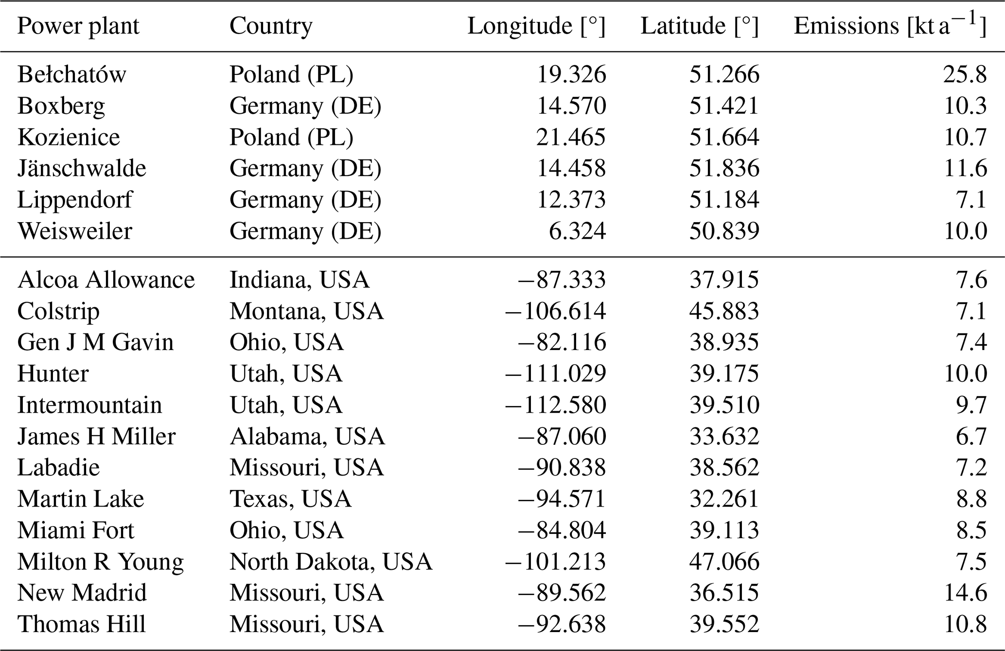
Figure 1 provides an illustration of the different steps of our approach. The plume area used for fitting the Gaussian curve is defined by following the wind direction from 1 to 30 km downwind of the source. In the across-wind direction, the plume area extends ±40 km perpendicular to the wind direction (Fig. 1a). This spatial window ensures that the plume is sufficiently captured while minimizing interference from neighboring sources or background variability.

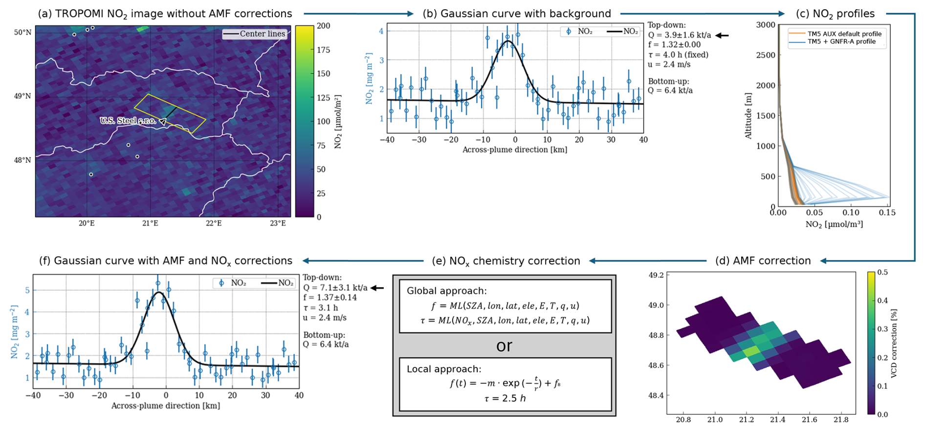
Figure 1 Top-down emission quantification method: (a) TROPOMI NO₂ image with 30 km long and 80 km wide plume area in yellow. (b) Gaussian curve with background (Eq. 3) fitted to the NO₂ columns in the plume area. (c) NO₂ profiles from the auxiliary default profiles from TM5 and profiles with added enhancement from Gaussian curve fit following the GNFR-A emission profile. (d) AMF correction for the pixels in the plume area using the updated profiles. (e) NO_x chemistry correction for f and τ using global or local approach. (f) Gaussian curve with background after AMF correction and final emission estimate Q with NO_x chemistry correction.

3.3 Air mass factor corrections

The air mass factors (AMFs) provided in the standard TROPOMI product are known to be biased in regions with strong local enhancements (Griffin et al., 2019; Verhoelst et al., 2021; Douros et al., 2023). This is because the global TM5 chemistry transport model, which provides the NO₂ profiles, has a coarse horizontal resolution of 1°, which is not sufficient to resolve narrow NO₂ plumes from individual point sources.

To address this limitation, we apply a correction to the AMFs using the averaging kernels (AKs) provided in the standard product and a modified vertical NO₂ profile (Eskes and Boersma, 2003). First, we fit the Gaussian curve with the linear background (Eq. 3) to the uncorrected NO₂ image (Fig. 1b). Next, we enhance the standard TM5 NO₂ profile by adding the fitted NO₂ enhancements to the TM5 profile of each pixel. The enhancements are vertically distributed according to the GNFR-A emission profile (Fig. 1c). Finally, we recalculate the AMFs by applying the AKs to the modified NO₂ profile. Figure 1d shows that this approach increases the VCDs in the plume center (by 30 %–40 % in this example), while background VCDs are not modified. The corrected AMFs are then used to update the NO₂ column densities. Subsequently, Eq. (3) is re-fitted to the corrected NO₂ columns to obtain the AMF-corrected line density q, which is used in the CSF method to compute the final NO_x emission estimates (Fig. 1f).

3.4 NO_x chemistry corrections

To derive NO_x emissions from NO₂ satellite observations, it is necessary to estimate the NO₂-to-NO_x conversion factor f and the NO_x lifetime τ. In this study, we use a global approach, which is based on global chemistry transport simulations with GEOS-Chem, and a local approach, which is based on plume-resolving simulations with the MicroHH large-eddy simulation (LES) model for the Jänschwalde power plant. We detail the two methods below.

3.4.1 Global approach: GEOS-Chem simulations

The emissions monitoring system developed for the CO₂MVS capacity will be based on the Integrated Forecasting System (IFS) operated by ECMWF (Inness et al., 2013). One of the envisioned capabilities of CO₂MVS is the assimilation of NO₂ satellite observations to constrain CO₂ emission using emission ratios. However, the greenhouse gas monitoring system will not perform full-chemistry simulations due to the high computational costs. Instead, a lightweight chemistry scheme based on machine learning would be used for predicting NO₂:NO_x concentration ratios and NO_x rate of change from meteorological variables available within the IFS.

As part of the CORSO project, a prototype of this scheme was developed for Europe using training data from the GEOS-Chem model. The machine learning model predicts NO₂:NO_x concentration ratios from solar zenith angle, longitude, latitude, height above surface, shortwave radiation, temperature, humidity and wind speed. To predict NO_x rate of change, the model additionally requires NO_x concentrations as input. This prototype model is described and validated in detail by Schooling et al. (2025).

In this study, we use an expanded version of the prototype, trained on global GEOS-Chem simulations for the year 2021 at a resolution of 2° by 2.5°. Meteorological input parameters for the machine-learning model were taken from ERA5 reanalysis. To estimate the NO_x rate of change, we converted the modified NO₂ profiles from the AMF calculation to NO_x using the predicted NO₂:NO_x concentration ratios from the machine-learning model. The NO_x lifetime is then calculated using $\mathit{\tau }=-\left[{\mathrm{NO}}_x\right]/R$, where [NO_x] is the NO_x concentration (in molec. cm⁻³) and R is the rate of change (in molec. cm⁻³ s⁻¹). Finally, the vertical profiles of ratios and lifetimes are weighted using the GNFR-A emission profile to compute column-averaged NO₂:NO_x ratios f and NO_x lifetimes τ (Fig. 1c and e)).

3.4.2 Local approach: MicroHH simulations

Recent high-resolution atmospheric chemistry simulations with the MicroHH LES model have shown that NO_x chemistry within emission plumes is highly complex, with chemical evolution strongly influenced by emission strength, wind speed, amount of turbulent mixing with the background atmosphere, and time since emissions (Krol et al., 2024). As a consequence, NO_x correction factors can vary significantly depending on the method and part of the plume used for emission quantification (Hakkarainen et al., 2024).

The MicroHH simulations were conducted for three power plants (Bełchatów in Poland, Jänschwalde in Germany, Matimba in South Africa) and one steel plant (Lipetsk in Russia). Due to the high computational cost of the simulations only 48 h could be simulated for each plant. Meier et al. (2024) analyzed these MicroHH simulations to improve the accuracy of NO_x emission estimates from TROPOMI NO₂ observations. Based on the simulations, an empirical formula was developed that predicts the NO_x:NO₂ ratio f as a function of time since emissions:

$$\begin{array}{}\text{(4)}& f\left(t\right)=m\cdot \exp \left(-{\displaystyle \frac{t}{r}}\right)+f_{\mathrm{0}},\end{array}$$

where m, r and f₀ are parameters fitted to the simulations. Furthermore, they also analyzed the lifetime in these simulation, which varied from 1 to 5 h with a mean value around 2.5 h for Bełchatów and Jänschwalde.

Since plume-resolving simulations for all power plants in this study are not available, we adopted the parameters derived for the Jänschwalde power plant (i.e.: m=1.6 ± 0.1, r=1638 ± 162 s, f₀=1.31 ± 0.01). The power plant was simulated for 22 and 23 May 2018 with an annual NO_x emission rate of 18 kt. This emission strength lies within the emission range of the power plants analyzed here, which is important because Krol et al. (2024) find that emission strength does impact the NO_x:NO₂ ratio. Additionally, we apply a fixed lifetime of 2.5 h for all sources.

This local approach allows us to explore the spatial and temporal generalizability of high-resolution plume simulations conducted at a single location. If we would use the parameters for the Bełchatów power plant, which was simulated with 30 kt a⁻¹, NO_x:NO₂ ratios would be about 10 % higher. Although the empirical formula was originally developed using data from only two simulation days, its application over a full year has already shown promising results with a significant reduction in the biases between bottom-up and top-down emission estimates for the Bełchatów and Jänschwalde power plants (Meier et al., 2024).

3.5 Quality filtering

To ensure the reliability of individual emission estimates, estimates were visually inspected to identify potential causes of failure in the quantification process. Based on this assessment, we excluded all cases where either the shift or the standard width of the fitted Gaussian curve exceeded 10 km. A large shift typically indicates a misalignment between the observed plume and the wind direction used to define the plume axis, while an excessively broad standard width suggests that the fitting algorithm may have captured a diffuse source region or background enhancement upstream of the actual emission source. We also filter out estimates for wind speeds lower than 2.0 m s⁻¹, because of the large relative uncertainty of the wind speed itself and the NO_x chemistry correction factors. In particular, the correction factors are exceeding 3 for the local approach under low wind speeds, which introduces substantial uncertainty and reduces the reliability of the emission estimates.

3.6 Monthly and annual emission estimates

Various approaches have been proposed to compute monthly and annual emission estimates from individual estimates (Santaren et al., 2025). One method involves fitting a smooth function through individual estimates to reconstruct a seasonal cycle, which can then be integrated to obtain monthly and annual means (Kuhlmann et al., 2020). However, we found that the time series of bottom-up reports is not consistently smooth, making this approach less suitable for our dataset. Another commonly used method applies weighted averaging based on estimated uncertainties, but this introduces bias because the uncertainties in the CSF method are proportional to the magnitude of the estimated emissions (see next section). As a result, lower emission estimates, associated with smaller uncertainties, would receive disproportionately high weights, resulting in an underestimation of the true emissions.

In this study, we therefore compute monthly emissions by calculating the arithmetic mean of all valid individual estimates for each month. We deliberately avoid weighted averaging for the reasons outlined above. To derive annual emissions, we linearly interpolate monthly means to fill gaps in months where no valid estimates are available. The final annual emission value is calculated as the median of the twelve monthly values. This approach mitigates the risk of bias from isolated extreme values, which can occur if only a single estimate is available in a given month, particularly in winter.

3.7 Uncertainties

The uncertainties in the top-down emission estimates are quantified using Monte Carlo simulations, which estimate the uncertainty by generating an ensemble of the input parameters for the CSF method. The Monte Carlo simulation assume that errors are uncorrelated, i.e., uncertainty reduces with the number of estimates. The uncertainty of line density q is derived from fitting the Gaussian curve using the precision of the TROPOMI NO₂ product. This precision is used to create an ensemble of line densities for each estimate. For wind speed, we assume an uncertainty of 1.0 m s⁻¹, consistent with the validation of the ERA5 reanalysis product (e.g., Vanella et al., 2022; Potisomporn et al., 2023). To avoid negative wind speeds in the ensemble, we use a lognormal distribution centered on the effective wind speed, with a standard deviation is 1.0 m s⁻¹.

Wind speed uncertainty has a direct impact on the uncertainty of the chemistry correction, because it is required to calculate the time since emissions used in Eqs. (4) and (2). For the local chemistry approach, we additionally include the uncertainties in the empirical parameters (m, r and f₀) used for the NO₂-to-NO_x conversion factor. The NO_x lifetime is modelled using a lognormal distribution with a mean of 2.5 h and a standard deviation of 0.6 h, consistent with the distribution in the two-day simulation for Jänschwalde (Meier et al., 2024). For the global approach, we use an uncertainty of 0.10 for the ratio, which was obtained by comparing the machine-learning with the GEOS-Chem simulations. The uncertainty in the rate of change is negligible compared to the uncertainty in the time since emissions; therefore, it is not included.

To quantify the uncertainties in the estimated emissions, we compute 16th, 50th and 84th percentile of the Monte Carlo ensemble, corresponding to the median and the ±1σ confidence interval. For monthly and annual estimates, we account for a temporal sampling error of 30 % for each estimate, which was estimated from the bottom-up time series and is consistent with previous studies (Hill and Nassar, 2019). The temporal sampling error is uncorrelated and decreased as the number of estimates increases. Finally, we account for a correlated error of 10 % in estimates that do not decrease with the number of estimates; this error is added to the uncertainty of the monthly and annual values.

4 Results

4.1 Example of emission at satellite overpass

The CSF method was applied to the six power plants in Europe and twelve power plants in the USA summarized in Table 1. Figure 2 shows three examples of NO_x emission estimates derived from TROPOMI NO₂ observations for the Jänschwalde (DE), Miami Fort (Ohio, USA) and Hunter (Utah, USA) power plants. The examples highlight some of the challenges associated with estimating NO_x emissions from satellite observations.

For the Jänschwalde power plant, the emission plume is clearly visible in the satellite image. Additional plumes from nearby plants (Schwarze Pumpe and Boxberg) can also be identified south of Jänschwalde. The plume area (yellow polygon), limited to 30 km downwind, effectively isolates the Jänschwalde power plant, minimizing the interference from neighboring sources. The across-plume NO₂ enhancement is well captured by the Gaussian curve, resulting in a top-down emission estimate of 16.2 ± 4.7 kt a⁻¹ using the local chemistry approach. This value is slightly larger but consistent with the bottom-up estimate of 13.5 ± 1.2 kt a⁻¹.

In contrast, the Miami Fort power plant example shows no discernible plume in the TROPOMI NO₂ image. On the day of observation, the reported emissions were very low with only 2.3 kt a⁻¹ and wind speeds were relatively high with 5 m s⁻¹, likely dispersing the weak plume below the detection limit. The top-down estimate was flagged as invalid, because both the center position and standard width of the Gaussian curve were larger than 10 km.

The third example is for the Hunter power plant and shows its emission plume with bottom-up reported emissions of 11.5 kt a⁻¹. There is also an additional enhancement from the Huntington power plant, which is located about 25 km north (point) of Hunter power plant (triangle) and has 6 kt a⁻¹ annual emissions. This case illustrates the complexity of accounting for NO_x chemistry in overlapping plumes. For an inert gas, like CO₂, the enhancements from multiple sources would simply add up, and the total emission estimate would reflect the sum of the individual contributions. However, for reactive species like NO_x, the chemistry correction introduces a non-linear effect. Since the correction factor is dominated by the decay term, a stronger correction is necessary for older plumes (cf. Sect. 4.3). In this example, the NO_x from Huntington is significantly younger than the NO_x from Hunter. Consequently, the NO_x correction, assuming an older plume, strongly overcorrects the emission estimate. The resulting top-down estimate is 36.7 ± 8.2 kt a⁻¹, which is substantially higher than the combined bottom-up emissions of the two power plants.

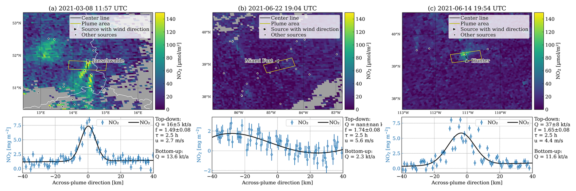
Figure 2 Three examples of NO_x emission estimates for (a) Jänschwalde, (b) Miami Fort and (c) Hunter power plant. The upper row shows the TROPOMI NO₂ image with location of the plume area. The lower row shows the NO₂ column densities in across-plume direction and the fitted Gaussian curve.

4.2 Annual emissions

Figure 3 and Table 2 compare the annual NO_x emission estimates from the bottom-up and top-down approaches for the 18 power plants. The bottom-up estimates are shown for the CAMS-GLOB-ANT inventory and the CORSO point source database. CAMS-GLOB-ANT emissions are integrated for the energy sector and all other sectors within a radius of 30 km around the power plant. CORSO emissions are shown for the power plant and for other facilities within a radius of 30 km. A radius of 30 km was used because top-down emissions are estimated using TROPOMI measurements from up to 30 km downstream of the facility. The top-down estimates use the local NO_x correction from the MicroHH simulations and the global correction from the GEOS-Chem simulations. To provide spatial context, Fig. 4 shows maps of total NO_x emissions from the CAMS-GLOB-ANT emission inventory and location of CORSO point sources in a 2° × 2° region around each power station.

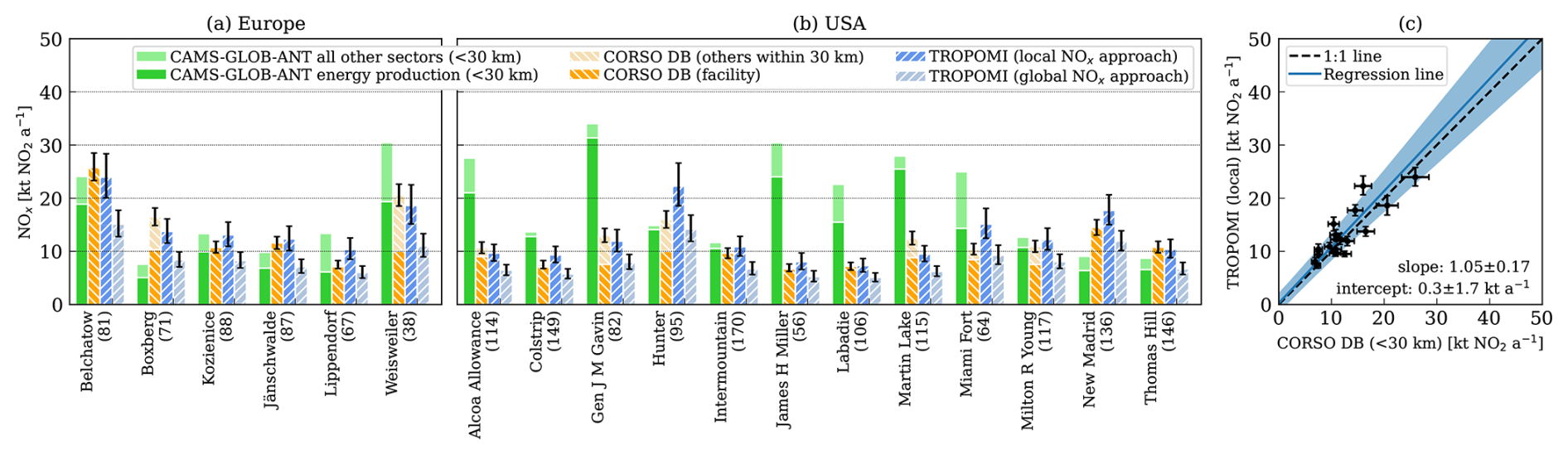
Figure 3 (a, b) Annual NO_x emissions from 18 power plants (in kt NO_x expressed as NO₂ a⁻¹), comparing bottom-up estimates from CAMS-GLOB-ANT (split between power generation and all other sectors) and the CORSO database, with top-down estimates derived from TROPOMI NO₂ observations using local and global chemistry correction approach. Numbers in brackets indicate the number of valid TROPOMI emission estimates in 2021 for each facility. (c) Scatter plot comparing bottom-up estimates from CORSO database (all within 30 km) with top-down from TROPOMI using local chemistry correction. For top-down estimates, error bars show 1σ confidence interval derived from Monte Carlo simulations.

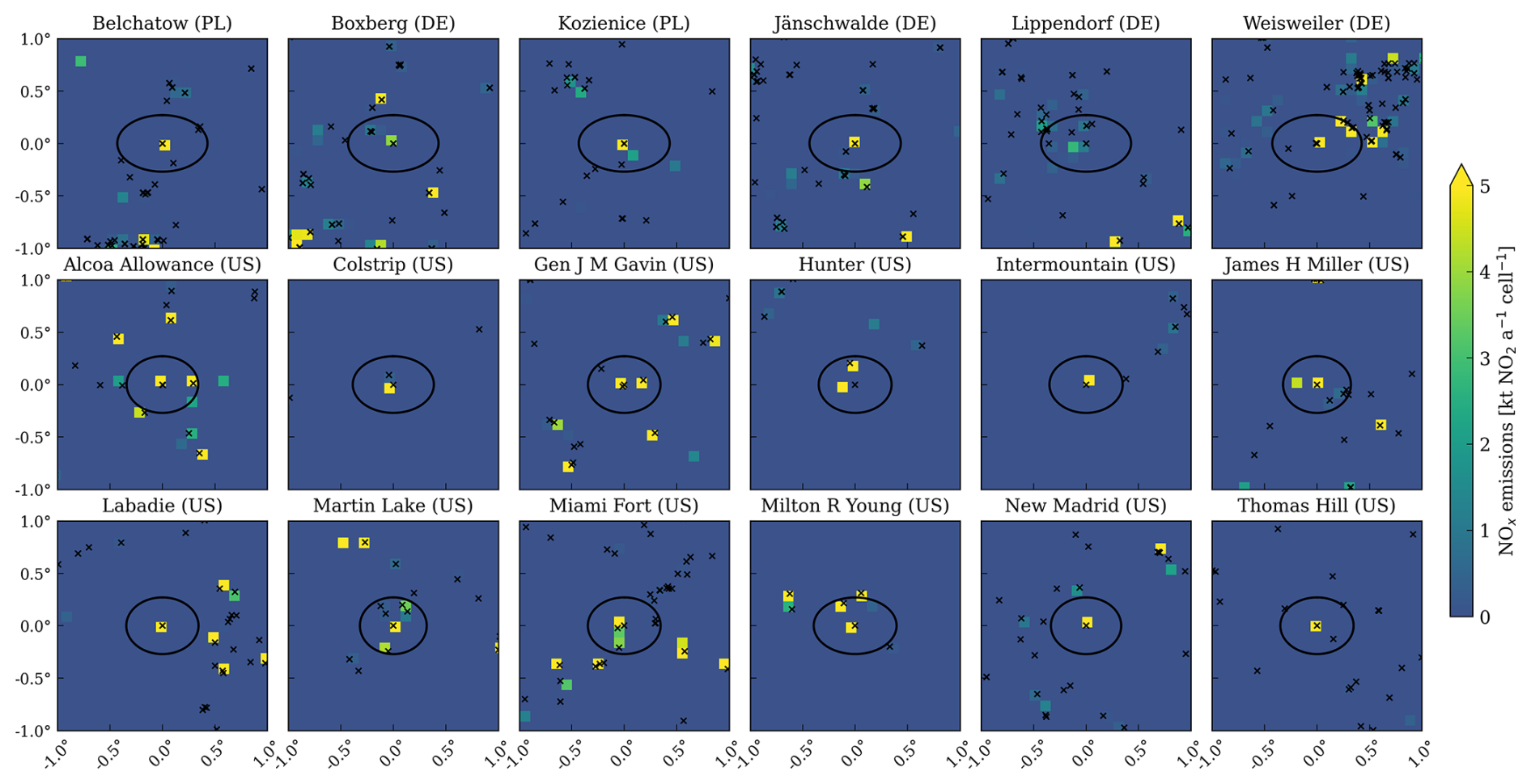
Figure 4 Emission maps of NO_x emissions in a 2° × 2° region around the power stations from the CAMS-GLOB-ANT inventory in 2021 (all sectors). Black crosses mark the locations of point sources in the CORSO database. The black circle shows a 30 km radius around the facility location.

Table 2 Annual top-down and bottom-up NO_x emission estimates in kt NO_x expressed as NO₂ a⁻¹.

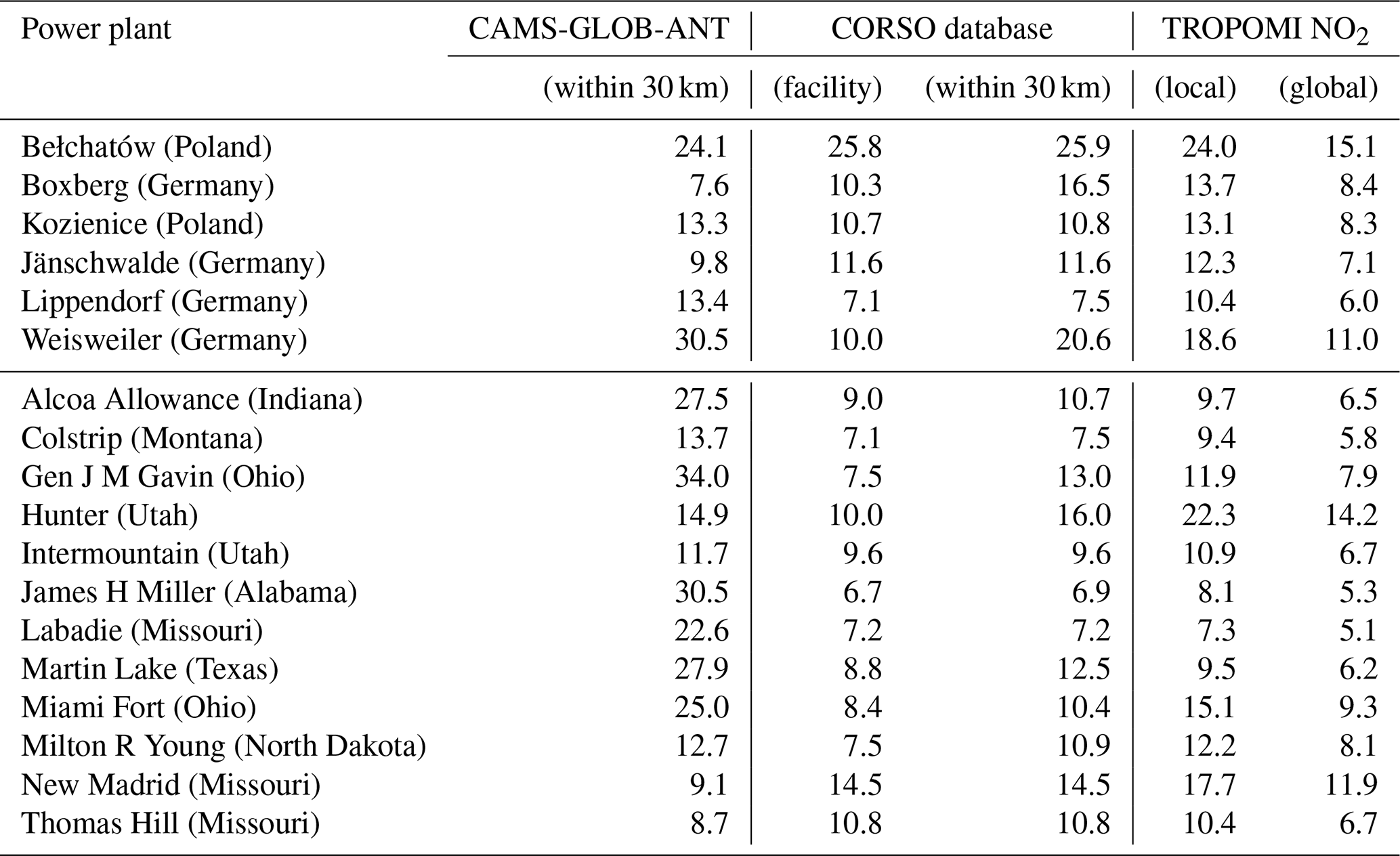
On average, total emissions from the CAMS-GLOB-ANT inventory are 70 ± 100 % larger than those reported in the CORSO database. The differences arise because CAMS-GLOB-ANT includes emissions not only from power plants, but also from other relevant NO_x combustion sources such as road transport, residential and commercial combustion and manufacturing industry, while CORSO is limited to major power plant, iron/steel production sites and cements plants. When considering only the CAMS-GLOB-ANT emissions reported for the power generation sector, differences with the CORSO database are much lower 30 ± 81 %, although significant discrepancies still exist at specific sites. For instance, emissions in CAMS-GLOB-ANT around Boxberg (Germany), which include the Schwarze Pumpe power plant, are only half of those reported in CORSO. Moreover, CAMS-GLOB-ANT includes emissions of some power plants that were decommissioned prior to 2021, such as the Gorgas power plant (reported at 4 kt a⁻¹ in CAMS-GLOB-ANT) east of James H Miller power plant in Alabama (Fig. 4), which was permanently closed in 2019. This is probably because the CAMS-GLOB-ANT is based on a version of the EDGAR inventory, which uses the outdated CARMA version 3 power plant database from 2009 (Soulie et al., 2024), whereas the CORSO database uses reported emissions from 2021. This issue has been resolved in more recent versions of EDGAR (Crippa et al., 2024). In addition, spatial mismatches are evident in CAMS-GLOB-ANT with emission locations sometimes offset from actual stack coordinates, for example, in the case of the Hunter power plant. This is also related to the use of CARMA in the EDGAR inventory. The spatial analysis also shows that several facilities are located near urban areas or industrial complexes, as observed for Lippendorf (Germany), Weisweiler, (Germany) Miami Fort (Ohio), and Labadie (Missouri).

The top-down estimates using the local NO_x correction approach are 58 ± 8 % higher than those obtained with the global approach, due to the larger correction factor of the local approach (see Sect. 4.3). When comparing CORSO bottom-up and top-down approaches for individual power plants, the local approach yields emissions 34 ± 34 % larger. However, satellite-based estimates are sensitive to the area surrounding the source. If we consider all point sources within 30 km of the power plant, the local approach is only 9 ± 20 % larger than bottom-up estimates. In contrast, the global approach still yields top-down estimates that are 31 ± 12 % lower than the bottom-up estimates within the same 30 km radius.

We find larger discrepancies for some power plants. One example is the Hunter power plant in Utah, which is located near the Huntington power plant (Fig. 2c), the NO_x correction appears to systematically overestimate emissions. Similarly, for the Miami Fort power plant in Ohio, top-down estimates exceed bottom-up values (cf. Table 2). This facility is also surrounded by several nearby point sources, which may contribute to the overcorrection effect similar to what was seen at Hunter. Additionally, emissions during the summer months at Miami Fort were low and frequently below the satellite detection threshold (Fig. 2b). Since non-emitting days are not included when averaging, this may lead to an overestimation of annual emissions.

Figure 3c shows that the regression between CORSO bottom-up estimates (within 30 km) and local top-down estimates yields a slope of 1.06 ± 0.17 and an intercept of 0.3 ± 1.7 kt a⁻¹, with a correlation coefficient of approximately 0.70, showing good agreement.

4.3 Impact of NO_x chemistry

To assess the influence of the NO_x chemistry on estimated emissions, Fig. 5 shows the temporal variability and the relationship between wind speed and the chemistry parameters (f, $\mathrm{1}/D$ and $c=f/D$) for the Jänschwalde power plant in Germany. A second version of the figure with narrower y-axes is provided in the Supplement.

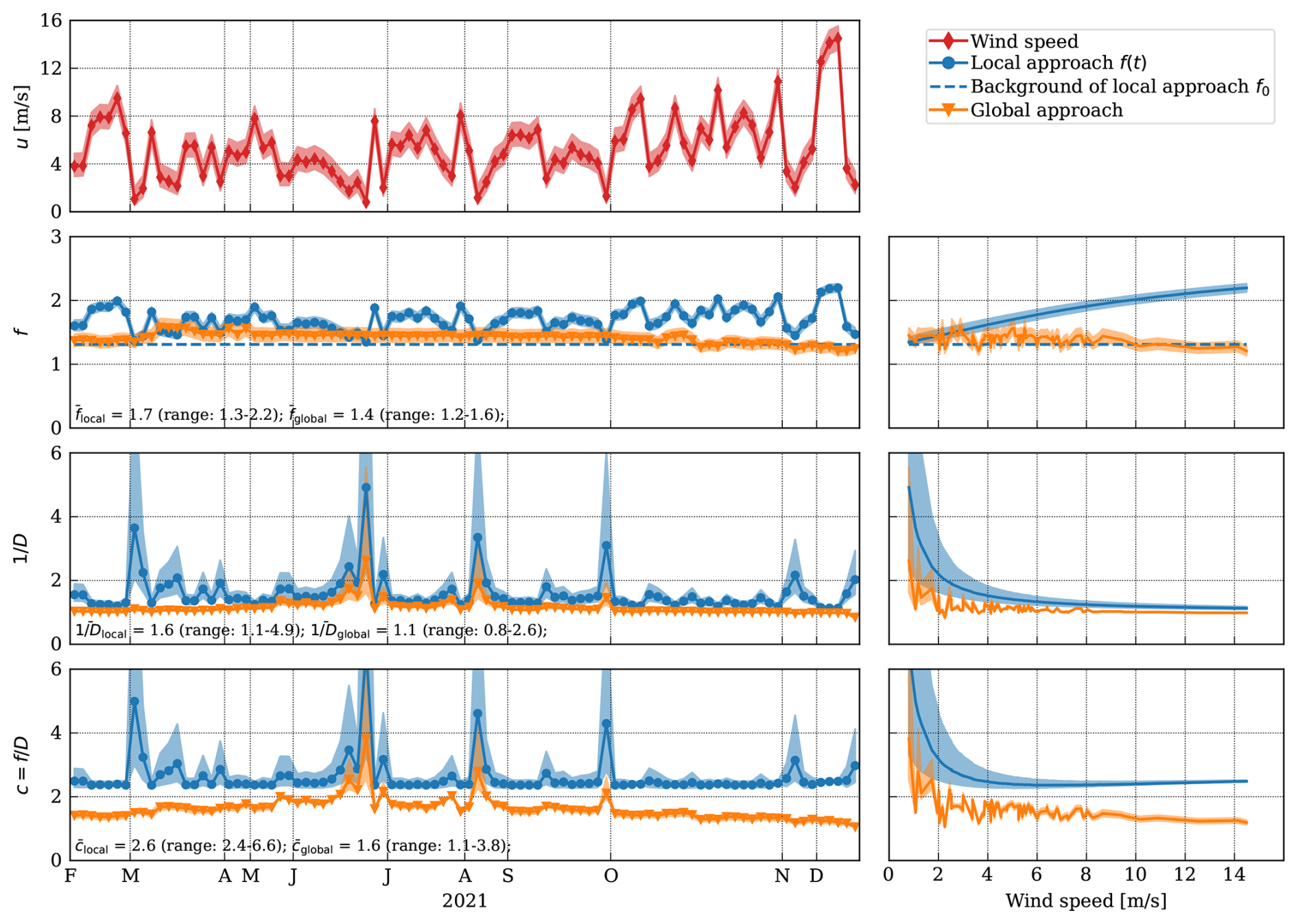
Figure 5 Comparison of NO_x chemistry parameters used for estimating NO_x emissions from TROPOMI NO₂ observations for the Jänschwalde power plant, using the local and global correction approach. Rows show wind speed u, NO₂-to-NO_x conversion factor f, NO_x decay correction term D (Eq. 2), and the combined correction $c=f/D$. The left column displays the time series of each parameter, while the right column shows the same data sorted by wind speed. The shaded area shows the 68 % confidence interval (CI) derived from the Monte Carlo simulations.

The conversion factor, f(t), derived from the local MicroHH simulations, shows strong temporal variability. This variability is driven by changes in wind speed, which affect the estimated time since emissions in Eq. (4) for a fixed plume area up to 30 km downstream. At low wind speeds, the plume remains longer in the area, allowing more time for converting NO to NO₂, resulting in lower conversion factors. Conversely, at higher wind speeds, less conversion occurs within the same area. Consequently, the conversion factor increases from 1.3 to 2.2 as wind speeds increase from 1 to 16 m s⁻¹. In contrast, the temporal variability of the conversion factor f for the global approach, based on GEOS-Chem, shows less temporal variability. The factor exhibits a weak seasonal cycle with smaller values during winter. However, it does not strongly depend on wind speed, as the approach lacks explicit information about time since emissions. The mean value of 1.4 is slightly larger than the background parameter f₀=1.31 from the MicroHH simulations.

The decay correction term $\mathrm{1}/D$ depends strongly on wind speed for both approaches, which is primarily driven by wind speed directly influences the time since emission in Eq. (2). In fact, a constant lifetime of 2.5 h was used for the local approach. The global approach has lifetimes of about 5 h in summer and even longer lifetimes in winter. As expected, the correction term is largest for low wind speeds, because more NO_x has decayed within the 30 km plume length. For the local approach, the term ranges from 4.0 at 1 m s⁻¹ to 1.2 at 16 m s⁻¹. For the global approach, the correction term is smaller with a mean value of 1.1. The correction term can even become smaller than 1 in winter, indicating net NO_x production.

The combined term $c=f/D$ is dominated by the decay term with larger values for low wind speeds. It ranges from 2.4 to 6.6 for the local approach and 1.1 to 3.8 for the global approach. The difference explains the systematic offset between the emission estimates using the two approaches. Importantly, the large correction factor associated with low wind speeds was the reason for filtering out top-down estimates with wind speeds below 2 m s⁻¹, because they introduce substantial uncertainty and potential overestimation.

4.4 Time series of emissions

The number of valid satellite overpasses per year ranges from 38 to 170, depending on the cloud frequency at the location and the isolation of the power plant. Fewer estimates are available for plants situated near other emission sources, as overlapping plumes and interference often lead to quality filtering and data rejection. For all European power plants, the number of valid top-down emission estimates during winter is notably low, with only 12 % of the total valid estimates occurring in that season. In January 2021, the Kozienice power plant in Poland is the only plant providing a valid estimate. For U.S. power plants, slightly more valid estimates (16 %) are available during winter (see Fig. S4 in the Supplement).

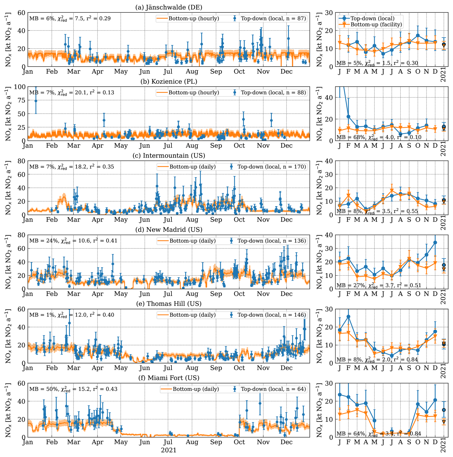
Figure 6 Time series of NO_x emission estimates from top-down (using the local NO_x correction approach) and bottom-up (based on reported values for the power plant). The left column shows individual satellite overpass estimates (n indicates the number of overpasses used), while the right column presents monthly averages. Error bars represent the 1σ confidence interval derived from Monte Carlo simulations. Numbers show relative mean bias (MB in %), reduced chi-squared values (${\mathit{\chi }}_{\mathrm{red}}^{\mathrm{2}}$) and Pearson correlation coefficient (r²) for each time series.

Figure 6 compares top-down and bottom-up NO_x emission time series for six selected power plants. The time series for all analyzed plants are shown in the Supplement. The left column displays individual estimates, while the right column shows monthly values. For European power plants, bottom-up estimates are derived from the CORSO annual values scaled by power generation data, whereas for U.S. plants, daily NO_x emissions directly taken from CEMS measurements. We further computed relative mean bias (MB in %), reduced chi-squared values (${\mathit{\chi }}_{\mathrm{red}}^{\mathrm{2}}$) and Pearson correlation coefficient (r²) for each time series.

For the Jänschwalde power plant, top-down estimates are slightly larger than bottom-up reports (MB ≈ 5 %). The correlation coefficients are low (r² ≈ 0.3) preliminary due to the low variability of emissions of the plant. The reduced chi-squared value is moderately high for individual estimates (${\mathit{\chi }}_{\mathrm{red}}^{\mathrm{2}}=\mathrm{7.5}$), while the monthly value (${\mathit{\chi }}_{\mathrm{red}}^{\mathrm{2}}=\mathrm{1.5}$) is close to unity, suggesting that the differences between bottom-up and top-down estimates are broadly consistent with their estimated uncertainties. The time series for the Kozienice power plant shows generally similar performance, except for a pronounced outlier in January. This outlier was not flagged by the automatic quality filtering, resulting in a large mean bias for monthly values and, consequently, lower reduced chi-squared values and correlation coefficients (MB =68 %, ${\mathit{\chi }}_{\mathrm{red}}^{\mathrm{2}}=\mathrm{4.0}$, r²=0.10). This highlights the importance of robust quality filtering in top-down approaches.

The four U.S. power plants exhibit strong variability in reported emission, which is reflected in the top-down estimates and results in high correlation coefficients (r² ranging from 0.51 to 0.84 for monthly values). The mean bias is small for Intermountain and Thomas Hill (8 %) but larger for New Madrid (27 %). Reduced chi-squared values range from 10 to 20 for individual overpasses and fall below 4 for monthly values, generally indicating good agreement at the monthly scale. The Miami Fort power plant has a strong seasonal cycle with very low emissions reported from May to October. Top-down estimates capture this pattern, although the number of valid estimates is limited during summer, because emissions frequently fall below the detection limit (e.g., Fig. 2b). While the correlation coefficient is high (r²=0.84 for monthly values), the mean bias is quite large (MB =64 %) due to the presence of other sources in the vicinity (see Fig. 4). This bias is reduced when considering all point sources within 30 km (Table 2).

Figure 7 shows MBs, ${\mathit{\chi }}_{\mathrm{red}}^{\mathrm{2}}$ and r² for individual estimates and monthly mean values (see Table S1 in the Supplement for all values). Since we compare bottom-up emissions for the power plant, MBs can be large when plants are not isolated because top-down values are sensitive to surrounding sources, (cf. Fig.4). The correlation coefficients span a large range, with low values for plants without a pronounced seasonal cycle and higher values for monthly averages. Reduced chi-squared values are generally below 5 for monthly values (${\overline{\mathit{\chi }}}_{\mathrm{red}}^{\mathrm{2}}=\mathrm{3.9}$, range: 1.5 to 11.5), with remaining deviation between top-down and bottom-up driven by the mean bias, due to missing neighboring sources, and uncertainties in the top-down method such as uncertainties in NO₂ columns (e.g., AMF correction), wind speed and NO_x chemistry correction.

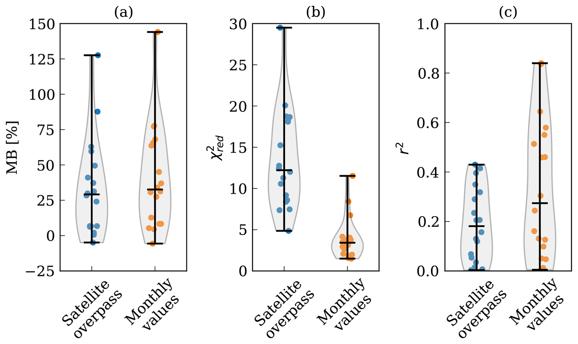
Figure 7 (a) Relative mean biases (MB), (b) reduced chi-squared values (${\mathit{\chi }}_{\mathrm{red}}^{\mathrm{2}}$) and (c) Pearson correlation coefficients (r²) comparing the time series of bottom-up and top-down NO_x emissions at satellite overpass and for monthly values.

5 Discussion and conclusions

This study investigates the potential of satellite-based TROPOMI NO₂ observations to quantify the seasonal and daily variability of NO_x emissions from point sources. We focus on eighteen power plants in Europe and the United States of America. Top-down emissions were derived using the cross-sectional flux method implemented in the ddeq Python library. To account for NO_x chemistry, we compared two approaches for converting NO₂ to NO_x and for correcting for NO_x lifetime: a “local” correction extrapolated from plume-resolving MicroHH simulations, and a “global” correction interpolated from GEOS-Chem simulations using a machine learning model. We evaluated the top-down estimates against bottom-up estimates from the CAMS-GLOB-ANT and the newly developed CORSO point source database. The CORSO database uses emissions data officially reported by the EEA in Europe and the EPA in the USA, providing more accurate representation of point sources. In contrast, the CAMS-GLOB-ANT inventory is based on the EDGAR inventory, which relies on country-level activity data and emission factors, making it less reliable for facility-level comparison.

Our results show that annual NO_x emissions can be determined from TROPOMI NO₂ observations with good accuracy when using the local correction approach and by aggregating all CORSO point sources within a 30 km radius to account for spatial representativeness. The comparison between the local and global correction approaches highlights the importance of resolving NO_x chemistry at the plume scale. The local correction approach generally yields higher emissions due to larger correction factors, resulting in better agreement with the bottom-up estimates. The NO₂-to-NO_x conversion factor of 1.70 ± 0.08 and the lifetime correction of 1.58 ± 0.38 at about 15 km downstream of the source are larger than the values of 1.38 ± 0.10 and 1.34 ± 0.25 used by Beirle et al. (2023). Consequentially, our estimates with the local approach are about 70 % larger than Beirle et al. (2023) (cf. Fig. S5 in the Supplement).

The accuracy of the corrections based on the MicroHH simulations for the Jänschwalde power plant in Germany depends on the representativeness of the underlying two-day simulations for the other power plants in this study. Since our study focused on Europe and the USA, regions with similar chemical environments, this approach seems to generalize reasonably well. Nevertheless, further work is needed to assess the applicability in regions with different chemical regimes using dedicated simulations. These simulations can be validated using satellite NO₂ observations, for example, by estimating NO_x decay times from TROPOMI, which is possible for long plumes but requires careful data selection.

The spatial representativeness with a radius of 30 km was chosen because TROPOMI NO₂ observations were used up to 30 km downstream of the source. In practice, the spatial sensitivity might be smaller and depend on the alignment of the sources with wind direction. The top-down approach is sensitive to the source in the radius depends on alignment of sources with wind direction, and the area might actually be smaller. Overlapping plumes from nearby sources present an additional challenge. Due to the dependency of NO_x chemistry on the time since emissions, such overlaps can lead to systematic overcorrection and overestimation of emissions. To improve the comparison, it might be necessary to have spatial representivness depend on wind direction using a smaller radius, resulting in lower values, and improve NO_x correction, likewise resulting in lower values.

Temporal variability in bottom-up emissions from the CORSO database was derived using electricity generation data for Europe and CEMS for the USA. This variability is captured in satellite-based NO_x estimates, although some limitations remain. Specifically, the detection limit of TROPOMI and the occurrence of non-emitting days can result in under-sampling and potentially overestimation of monthly or annual emissions if not properly accounted for. Winter months pose additional challenges due to frequent cloud cover, which reduces the number of valid satellite observations and increases uncertainty during periods of high variability in emissions. Despite these challenges, our results demonstrate that satellite observations can effectively resolve seasonal variability in NO_x emissions at the facility level. However, resolving short-term fluctuations from individual satellite images, which are typically only available once or a few times per day, remains more difficult due to data gaps and the high level of uncertainty in individual estimates. This necessitates careful filtering and verification of each estimate.

To support the development of a robust emissions monitoring system, improvements are needed in several areas: (1) better treatment of source clusters and overlapping plumes, (2) refined NO_x chemistry corrections that can be applied globally, and (3) enhanced quality filtering that reliably flags invalid estimates while retaining cases with emissions below the detection limit. Addressing these challenges would enable the quantitative use of NO₂ observations for monitoring NO_x emissions and for constraining co-emitted species such as CO₂. This is particularly relevant for upcoming satellite missions such as CO₂M (Sierk et al., 2021), GOSAT-GW (Tanimoto et al., 2025) and TANGO, which will measure both CO₂ and NO₂, as well as for geostationary air quality missions, such as GEMS, TEMPO and Sentinel-4, aiming to provide high temporal resolution of emissions.

While this study focused on power plants in Europe and North America – regions with relatively well-documented emissions from stack measurements – the same top-down framework can be applied to power plants in regions where bottom-up estimates are more uncertain, as well as to other hot spots such as urban areas and industrial facilities. This broader application is already supported by the ddeq Python library, which allows the user to adapt and modify the approach. For urban applications, different vertical NO₂ profiles need to be used for AMF corrections and the effective wind speed, and the NO_x chemistry correction would need to be adapted for urban plumes. Overall, this study demonstrates that satellite observations offer a unique opportunity to constrain emissions and highlights their crucial role in improving global emission inventories for cities, power plants, and a wide range of industrial sources.