Atmospheric CO₂ dynamics in a coastal megacity: spatiotemporal patterns, sea–land breeze impacts, and anthropogenic–biogenic emission partitioning

Attributing observed carbon dioxide (CO₂) to fossil-fuel emissions versus biogenic fluxes is essential for assessing urban mitigation, but in coastal megacities it is complicated by anthropogenic–biogenic coupling and sea–land breeze (SLB) circulation. Here we analyze Guangzhou using multi-site in situ CO₂ and CO measurements (January 2023–September 2024), transport footprints, and a site-specific ΔCO $/$ ΔCO₂ (R_CO) relationship to resolve spatiotemporal variability, quantify SLB effects, and partition fossil-fuel (CO₂ff) and biogenic (CO₂bio) contributions without assimilating emission inventories. Along a coastal–urban–suburban gradient, the coastal site shows the largest seasonal amplitude, the vegetated site exhibits strong summertime diurnal amplitude, and the urban core is combustion-dominated. These gradients reveal a “coastal CO₂ dome” that – unlike urban domes often conceptualized as core-anchored – is seasonally displaced, with peak concentrations shifting away from the core due to the interplay of coastal ventilation and biogenic exchange. SLB effects are seasonal: SLB ventilates CO₂ in spring–winter but promotes summertime accumulation (+2.08 ppm) under stable stratification, accompanied by pronounced CO enhancements, consistent with trapped/recirculated combustion plumes. Regression-derived urban R_CO is consistent with post-2013 broad tightening of coal/industrial and vehicle-emission controls. Winter-afternoon urban CO₂ff attribution remains robust to transport-model configurations and measurement/background uncertainty. Summer-afternoon CO₂bio shows substantial biogenic uptake, offsetting ∼ 60 % of concurrent CO₂ff. These results demonstrate that coastal dynamics and urban greening reshape observed CO₂ signals, highlighting that biogenic–anthropogenic decoupling and SLB-aware sampling are essential for the robust evaluation of carbon mitigation in coastal megacities.

1 Introduction

Atmospheric carbon dioxide (CO₂), the predominant anthropogenic driver of climate change, is accumulating at unprecedented rates in human history (WMO, 2024). Future CO₂ increments will exert stronger warming effects than equivalent past increases due to climate system feedbacks (He et al., 2023), making emission control imperative. Despite covering only 3 % of global land, urban areas generate over 70 % of carbon emissions (Crippa et al., 2021), positioning cities as critical arenas where mitigation policies, infrastructure transitions, and urban greening can drive measurable changes in urban carbon budgets (WMO, 2025).

Urban atmospheric CO₂ concentrations provide a complementary constraint to flux- or inventory-based assessments because they integrate surface emissions, biogenic exchange, and atmospheric transport over the upwind source area (Lin et al., 2003; Shusterman et al., 2018; Pitt et al., 2022). This integration, however, creates an attribution challenge because observed CO₂ variability reflects coupled effects of fossil-fuel emissions, biogenic fluxes, and meteorology/transport, and thus is not uniquely attributable to any single driver, although one factor may dominate in certain regimes, especially on diurnal to seasonal timescales (Xueref-Remy et al., 2018; Yang et al., 2021; Mitchell et al., 2018). The challenge is particularly acute in coastal megacities, where land–sea thermal contrasts and marine background inflow drive strong diurnal reversals in advection and boundary-layer structure (Leroyer et al., 2014; Lei et al., 2024). These dynamics complicate observational representativeness and source–sink separation, and can make inferred CO₂ enhancements sensitive to background selection under different transport regimes (Verhulst et al., 2017). Given their high exposure to climate-related hazards, especially flooding and storm impacts, coastal megacities are priority targets for climate-risk management, motivating robust, policy-relevant CO₂ emissions assessment (Kumar, 2021).

A range of approaches has been used to constrain urban carbon budgets, including bottom-up inventories, tower-based atmospheric observations, tracer/isotope measurements, and atmospheric inversions. Bottom-up inventories provide essential baselines, yet urban emissions remain uncertain and can differ across products because they depend on activity/emission-factor assumptions and proxy-based downscaling (Gately and Hutyra, 2017; Gurney et al., 2019). While radiocarbon (¹⁴C) measurements provide robust fossil-fuel/biogenic partitioning (Turnbull et al., 2015; Berhanu et al., 2017; Wang et al., 2022), their high cost and discontinuous sampling limit their applicability for long-term, high-frequency monitoring. Similarly, eddy covariance (EC) measurements quantify net CO₂ fluxes within tower footprints (typically 1–2 km radius), yet the derived flux partitioning reflects only local-scale dynamics and cannot fully represent city-wide carbon exchange processes (Velasco et al., 2013; Menzer and McFadden, 2017; Wu et al., 2022b). Fully three-dimensional (3-D) atmospheric inversions can assimilate concentration data to estimate city-scale emissions and quantify posterior uncertainty when observation networks adequately constrain boundary inflow and key transport uncertainties (Lauvaux et al., 2016; Lian et al., 2023). Yet in practice, urban inversions are often limited by incomplete observational coverage, representativeness (sub-grid) errors, and transport biases (Boon et al., 2016; Deng et al., 2017; Ye et al., 2020; Che et al., 2022b). They can also remain sensitive to choices of background/boundary conditions and prior assumptions, including those related to biogenic fluxes, which can be large and temporally variable during the growing season (Turnbull et al., 2018; Nalini et al., 2022; Ye et al., 2020). These constraints motivate complementary observation-driven frameworks that emphasize process-level interpretation of concentration variability while explicitly tracking uncertainty sources.

A defining coastal process is the sea–land breeze (SLB), a common mesoscale circulation driven by land–sea thermal contrast (Shen et al., 2021). In the Pearl River Estuary (PRE), SLB occurrence shows pronounced seasonality and spatial dependence, with spring–autumn maxima reported in parts of the region (You and Chi-Hung Fung, 2019; Mai et al., 2024b). SLB produces a clear diurnal reversal between onshore and offshore flow and can modify boundary-layer structure and mixing depth (Wu et al., 2013; Lei et al., 2024), complicating the interpretation of urban CO₂ variability. By contrast, inland basins/valleys lack marine inflow–outflow and may be shaped by lake–land breeze circulations (Yang et al., 2022) or other topography-modulated flows that can shift background conditions and the footprint representativeness of urban observations (Mitchell et al., 2018; Wang et al., 2021). Beyond the PRE, China's coastal basins exhibit distinct SLB seasonality (e.g., a summer maximum in the Bohai Rim, weak seasonality in the Yangtze River Delta, and an autumn maximum in the PRE) (Huang et al., 2025), likely driven by regional differences in large-scale wind fields and air–sea turbulent heat fluxes (Shen et al., 2024), and potentially modulated by coastline geometry and topographic constraints. Despite recognized impacts of SLB on air quality (Zhao et al., 2022; Wang et al., 2023; Zheng et al., 2024), only a few case studies have examined how SLB-driven recirculation of nocturnally respired CO₂ can perturb daytime coastal CO₂ measurements and may bias emission inversions (Ahmadov et al., 2007), and systematic quantification across coastal cities remains limited.

Urban greening reinforces the need for explicit source–sink separation because neglecting biogenic contributions can bias inferred urban emissions (Miller et al., 2020; Ye et al., 2020; Sargent et al., 2018). Moreover, urban vegetation is often highly fragmented and can be underrepresented in moderate-to-coarse remote-sensing land-cover/canopy products, which may miss fine-scale urban heterogeneity and thereby introduce additional uncertainty (and potential bias) into satellite-driven biogenic flux estimates (Ma et al., 2022; Corro et al., 2025; Glauch et al., 2025). Green coverage within built-up urban areas is similarly high across major Chinese coastal megacities (e.g., Guangzhou: 43.7 % in 2023; Shenzhen: 44.0 % in 2023; Qingdao: 44.0 % in 2023; Tianjin: 38.2 % in 2023) (Guangzhou Municipal Bureau of Statistics, 2024; Shenzhen Municipal Bureau of Statistics, 2024; Qingdao Municipal Bureau of Statistics, 2024; Tianjin Municipal Bureau of Statistics, 2024), implying that biogenic exchange can be non-negligible when interpreting urban observations. For example, in coastal North American cities, high-resolution vegetation modeling in New York City indicates that summertime biogenic uptake can offset up to 40 % of afternoon anthropogenic CO₂ enhancements and can fully balance on-road traffic contributions (Wei et al., 2022), while a dense-sensor analysis in Los Angeles suggests that daytime biogenic exchange can consume up to 60 % of fossil-fuel emissions during the peak growing season (Kim et al., 2025). Recent advances, including emerging atmospheric constraints such as carbonyl sulfide (COS), further demonstrate the feasibility and value of more robust biogenic quantification in city carbon budgets (Soininen et al., 2025).

Taken together, three knowledge gaps limit the interpretation of coastal megacity CO₂ observations and their use for mitigation assessment: (i) how spatiotemporal CO₂ patterns vary across a coastal–urban–suburban gradient; (ii) how SLB-driven transport and boundary-layer mixing reshape diurnal and seasonal CO₂ signals through seasonally varying ventilation, boundary-layer depth, and atmospheric stability, which may differ from inland-city regimes; and (iii) how fossil-fuel and biogenic contributions can be robustly separated, with quantified uncertainty, in a coastal setting. To bridge these gaps, we investigate Guangzhou (Pearl River Delta, China) as a living laboratory: high GDP and population indicate strong energy and mobility demand and thus substantial fossil-fuel CO₂ emissions, while evergreen urban vegetation, a long growing season, and frequent SLB circulation can produce non-negligible biogenic signals and complex coastal transport. The policy context further elevates the value of attribution: Guangdong's emissions-trading system (ETS) has operated since 2013, alongside measures targeting energy structure, vehicle emissions, building efficiency, and urban greening.

Given this imperative to track changes in urban emissions and net carbon exchange, we use an observation-driven framework that complements atmospheric inversion approaches and interprets diurnal–seasonal variability by combining multi-site in-situ CO₂ and CO measurements with footprint-informed transport analysis (Lin et al., 2003; Fasoli et al., 2018). Unlike a formal Bayesian 3-D inversion, our framework targets process attribution of observed variability and quantifies robustness through sensitivity tests rather than posterior flux estimates. This approach emphasizes process-level interpretation of concentration variability while explicitly evaluating key uncertainty sources. While CO is widely used to infer fossil-fuel CO₂, it carries inherent uncertainties due to varying emission ratios (R_CO), background variability, and atmospheric chemical processing (Turnbull et al., 2011; Chen et al., 2020; Griffin et al., 2007; Vimont et al., 2019). Footprint estimates are likewise sensitive to meteorological forcing and boundary-layer representation, and such transport sensitivities may be amplified under complex coastal mesoscale flows. We therefore quantify uncertainties associated with measurement and background selection, evaluate robustness to transport-model setup via STILT configuration tests, assess biogenic consistency using seasonal vegetation activity (e.g., NDVI), and utilize emission inventories for contextual comparison – using inter-inventory spread as a plausibility envelope for benchmarking rather than a validation target.

Accordingly, we aim to: (i) resolve spatiotemporal patterns of CO₂ across three sites spanning near-coastal (NS), urban-core (PY), and suburban (CH) environments; (ii) quantify how SLB modulates diurnal–seasonal CO₂ variability and interpret the contrasts in terms of changes in wind ventilation, boundary-layer depth, and seasonally varying atmospheric stability/stratification; and (iii) partition observed CO₂ enhancements at the urban site (PY) into fossil-fuel and biogenic components using CO and footprint information, with explicit uncertainty characterization via measurement/background terms and STILT configuration sensitivity tests.

2 Data and methodology

2.1 Observational sites

The high-precision greenhouse gas monitoring network in Guangzhou is illustrated in Fig. 1. Three stations – Nansha (NS), Panyu (PY), and Conghua (CH) are symmetrically distributed along the city's predominant south–north wind axis, representing coastal, urban, and suburban atmospheric conditions, respectively. Site selection criteria are detailed in the Supplement. All stations employ tower-based sampling at similar heights: NS and PY at 48 m, and CH at 40 m. Monitoring spanned from 1 January 2023 to 30 September 2024. From PY, the straight-line distances to NS and CH are 54 and 89 km, respectively.

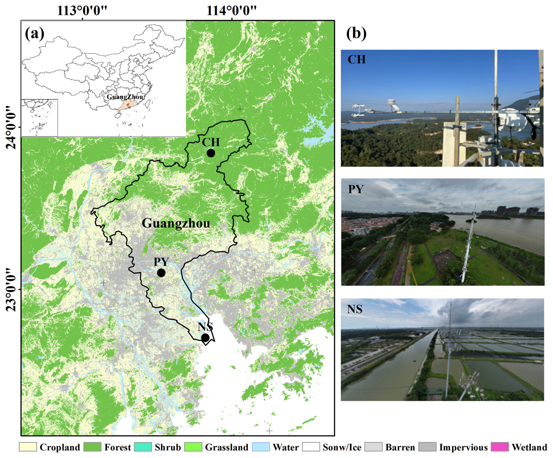
Figure 1 (a) Geographic locations of the NS, PY, and CH stations, with regional land use classification based on the 30 m resolution 2023 land cover product of China (CLCD) (Yang and Huang, 2025). (b) Photographs of each station.

The NS station (113.63° E, 22.61° N) is located < 5 km from the coastline. This coastal site is surrounded by aquaculture ponds and sparse wetlands. Infrastructure nearby includes the under-construction southern extension of Guangzhou Metro Line 18 (NW direction) and the S78 highway (∼ 2 km west). The PY station (113.38° E, 23.03° N) is situated in the densely populated urban core; the tower is adjacent to Guangzhou University Town (north) and the Pearl River (south). A city road (∼ 100 m north) and the S73 expressway (∼ 700 m west) contribute to local emissions. The CH station (113.78° E, 23.74° N) is positioned in the northern suburbs. The site is bordered by subtropical evergreen broadleaf forests (north), a tourist resort (south), and a tea processing plant. The G45 highway lies ∼ 3 km northwest. According to the Emissions Database for Global Atmospheric Research (EDGAR) Community GHG database (EDGAR_2024_GHG; 2023; 0.1° × 0.1°) (Crippa et al., 2024), grid-level CO₂ emission densities for NS, PY, and CH are 3456, 15 244, and 203 t km⁻² yr⁻¹, respectively (Fig. S1 in the Supplement).

2.2 Monitoring system

All three stations are equipped with similar monitoring systems, consisting of sampling modules, calibration modules, gas analyzers, and data acquisition systems. Notably, the NS and PY stations utilize Picarro G2401 greenhouse gas analyzers to measure CO₂ $/$ CH₄ $/$ CO $/$ H₂O, with a CO₂ measurement precision of < 20 ppb (5 min, 1σ). The CH station employs an ABB GLA331-GGA greenhouse gas analyzer to measure CO₂ $/$ CH₄ $/$ H₂O, with a CO₂ measurement precision of < 25 ppb (5 min, 1σ). N₂O and CO are measured using a GLA351-N2OCM analyzer. Detailed monitoring system and principles of the instruments are provided in the Supplement. Prior to field deployment, comparative tests were conducted in the laboratory to ensure the analytical performance consistency of the instruments. Additionally, meteorological sensors (measuring wind speed, direction, humidity, temperature, and pressure) are installed at the same height as the sampling inlets at NS and PY stations, while the CH station lacks such sensors. Detailed descriptions of wind field characteristics at NS and PY stations are included in the Supplement and illustrated in Fig. S2.

2.3 Calibration methods

The calibration module comprises two components: working standard curve establishment and target gas verification. High- and low-concentration standard gases are used to establish calibration curves, while a mid-concentration standard gas is used for target verification. The target and calibration gases are stored in inert-coated aluminum cylinders, uniformly supplied by the China National Environmental Monitoring Center. All stations follow the same calibration protocol: (1) weekly calibration curve establishment: high- and low-concentration gases are injected for 30 min each, with the final 5 min of instrument response used for calibration; (2) target gas verification every 12 h: mid-concentration gas is injected for 30 min, with the final 5 min of response used for verification; (3) re-calibration is triggered if the residual value (H) from target verification exceeds ±0.2 ppm.

Calibration curves are derived from the instrument's response to calibration gas, yielding a linear calibration equation:

$$\begin{array}{}\text{(1)}& Y=A\times X-B,\end{array}$$

where A, B are calibration coefficients. Calibrated CO₂ (CO_2,k) is calculated by:

$$\begin{array}{}\text{(2)}& {\mathrm{CO}}_{\mathrm{2},k}=A\times {\mathrm{CO}}_{\mathrm{2},\mathrm{m}}-B,\end{array}$$

where CO_2,m is the measured response. Daily 12 h target gas verification is conducted to assess analyzer accuracy and stability by calculating the residual H:

$$\begin{array}{}\text{(3)}& H=\left(A\times {\mathrm{CO}}_{\mathrm{2},c}-B\right)-{\mathrm{CO}}_{\mathrm{2},n},\end{array}$$

where CO_2,n is the standard CO₂ concentration of the target gas, and CO_2,c is the analyzer response/reading to the target gas.

To ensure high-precision and stable monitoring results, periods with $\left|H\right|$ ≤ 0.1 ppm are prioritized. Measurement uncertainties for the analyzers at NS, PY, and CH stations, calculated as the standard deviation (SD) of H (Yang et al., 2021), are 0.04, 0.02, and 0.04 ppm, respectively. In addition to daily calibration, maintenance personnel conduct weekly inspections of instruments and station facilities, including checks on power supply stability, data logger functionality, and industrial control computer status. Consumables (e.g., filters) are replaced as needed, and emergency repairs or instrument overhauls are performed when necessary. Any instrument downtime caused by internal or external factors is documented in maintenance logs, and affected data is flagged. Throughout the monitoring period, all three stations maintained data validity rates exceeding 90 %.

2.4 Sea–land breeze identification

The straight-line distances from the NS, PY, and CH stations to the coastline are 4, 58, and 130 km, respectively. The NS station, closest to the coast, was selected to study Guangzhou's sea–land breeze (SLB) circulation. Prior to SLB identification, local and background winds must be differentiated, as tower-measured winds (Fig. S2 in the Supplement) represent superimposed local and background wind fields, where strong background winds can obscure SLB signals (Qiu and Fan, 2013). The following equations distinguish background winds from local winds (Sun et al., 2022; Shen et al., 2019):

$$\begin{array}{}\text{(4)}& {\displaystyle }{U}_{\mathrm{b}}=\stackrel{\mathrm{‾}}{\sum _{i=\mathrm{0}}^{\mathrm{23}}{U}_i},\text{(5)}& {\displaystyle }{V}_{\mathrm{b}}=\stackrel{\mathrm{‾}}{\sum _{i=\mathrm{0}}^{\mathrm{23}}{V}_i},\text{(6)}& {\displaystyle }{U}_{\mathrm{l}}=U_{\mathrm{o}}-U_{\mathrm{b}},\text{(7)}& {\displaystyle }{V}_{\mathrm{l}}=V_{\mathrm{o}}-V_{\mathrm{b}},\end{array}$$

where U_o and V_o are the observed wind fields from the tower, U_b and V_b denote background winds, and U_l and V_l represent local winds.

A sea–land breeze day (SLBD) is defined as any 24 h period exhibiting a distinct transition from sea breezes during the day to land breezes at night (Xiao et al., 2023). SLB identification criteria vary regionally due to differences in topography and coastline geometry (Huang et al., 2025). Guided by the SLB criteria in Table S1 in the Supplement and historical patterns for the Pearl River Estuary (Qiu and Fan, 2013; Zhang et al., 2024; Mai et al., 2024b), we define for the north-shore site (NS) directional sectors of 112–202° for the sea breeze and 302–45° for the land breeze. The corresponding detection windows are 12:00–20:00 LT (sea breeze) and 01:00–09:00 LT (land breeze), consistent with regional SLB climatologies. Directional persistence is evaluated using the local-wind direction. The wind-speed screen is applied to the observed wind-speed magnitude at 48 m. A day is labeled as an SLB day only if all the following conditions are satisfied: (1) Directional persistence: within each window, the local wind direction (from the decomposed local component) stays inside the corresponding sector for ≥ 4 h, or for ≥ 4 h within any running 5 h window; and (2) Weak-forcing screen: for the same candidate SLB day, the observed wind-speed magnitude at 48 m must remain < 10 m s⁻¹ at every hour of that day (i.e., no hourly value exceeds 10 m s⁻¹). This conservative cap follows coastal-China SLB climatologies and is intended to exclude strongly forced days (Qiu and Fan, 2013; Sun et al., 2022; Huang et al., 2025; Zhang et al., 2024). Otherwise, the day is designated a non-SLB day (NSLBD).

Together, these two requirements reduce the likelihood of misclassification under strongly forced conditions. Days dominated by synoptic forcing or tropical-cyclone peripheries often show a prolonged anomalous wind regime rather than a clear diurnal reversal (Atkins and Wakimoto, 1997; Allouche et al., 2023). To explicitly assess residual tropical-cyclone (TC) contamination, we cross-referenced the SLB calendar with 2023 Pearl River Delta (PRD)/Guangzhou TC impact windows compiled from the official Guangdong–Hong Kong–Macao Greater Bay Area (GBA) Climate Monitoring Bulletin (Table S2). For each TC, impact start/end are defined as the first/last local dates on which the bulletin reports PRD/Guangzhou impacts or advisories attributable to that system (including peripheral rainbands/gusts). Because the bulletin is date-based, we conservatively treat the entire day within each window as potentially TC-influenced. Only one SLBD (2 September 2023) falls within these windows; excluding it leaves results unchanged.

2.5 Estimation of CO₂tot, CO₂ff, and CO₂bio

The observed CO₂ concentration enhancements at tall-tower receptor sites represent the integrated influence of upwind surface fluxes transported by atmospheric advection and mixing (Lin et al., 2003). Consequently, upwind carbon emissions can be inferred from site-specific enhancement measurements coupled with their corresponding atmospheric footprints. Here we apply an observation-driven framework that combines concentration-enhancement observations with transport-model footprints to estimate total CO₂ (CO₂tot) and CO (COtot) surface fluxes, and to further derive fossil-fuel (CO₂ff) and biogenic (CO₂bio) components using the site-specific ΔCO $/$ ΔCO₂ relationship (R_CO), without relying on any a priori emissions inventory. The required inputs are limited to enhancement observations at the receptor sites and atmospheric footprints, consistent with previous regional flux quantifications for CO₂, CH₄, and CO (Mitchell et al., 2018; Lin et al., 2021; Wu et al., 2022a). Emission inventories are used only for site-context characterization (Sect. 2.1) and, subsequently, for an independent bottom-up plausibility envelope for winter-afternoon flux estimates (Sect. 3.5), rather than as priors or validation targets. CO₂tot and COtot are calculated as:

$$\begin{array}{}\text{(8)}& {\displaystyle }{\mathrm{CO}}_{\mathrm{2}}\mathrm{tot}={\displaystyle \frac{{\mathrm{CO}}_{\mathrm{2},s}\mathrm{obs}-{\mathrm{CO}}_{\mathrm{2}}\mathrm{bg}}{{\sum }_i{\mathrm{Footprint}}_{i,s}}},\text{(9)}& {\displaystyle }\mathrm{COtot}={\displaystyle \frac{{\mathrm{CO}}_s\mathrm{obs}-\mathrm{CObg}}{{\sum }_i{\mathrm{Footprint}}_{i,s}}},\end{array}$$

The numerators are hourly CO₂ and CO concentration enhancements (ΔCO₂ and ΔCO) at station s, where CO_2,sobs and CO_sobs represent observed CO₂ and CO concentrations, while CO₂bg and CObg denote urban background concentrations (detailed in the Supplement). The denominators are hourly total atmospheric footprints $\left({\sum }_i{\mathrm{Footprint}}_{i,s}\right)$, where i denotes backward particle release time from the receptor. Due to challenges in modeling mixed-layer depths during nighttime, morning, and evening, flux analysis focuses on afternoon hours (12:00–16:00 LT) (Boon et al., 2016; Mitchell et al., 2018; Lin et al., 2021). Daily-scale CO₂tot and COtot are derived by dividing the mean afternoon ΔCO₂ and ΔCO by the corresponding mean ${\sum }_i{\mathrm{Footprint}}_{i,s}$. The footprint quantifies the sensitivity of concentration enhancements at the observation site to upwind surface fluxes, as detailed in Sect. 2.5.1. ΔCO₂ is in units of [ppm], while footprint is in [ppm (µmol m⁻² s⁻¹)⁻¹], so CO₂tot, the quotient between the two quantities, is in flux units of [µmol m⁻² s⁻¹].

Anthropogenic CO₂ emissions (CO₂ff) are derived from COtot and the CO $/$ CO₂ emission ratio (R_CO), where R_CO is determined from real-time tower-measured data, as described in detail in Sect. 3.4:

$$\begin{array}{}\text{(10)}& {\mathrm{CO}}_{\mathrm{2}}\mathrm{ff}={\displaystyle \frac{\mathrm{COtot}}{R_{\mathrm{CO}}}},\end{array}$$

Biogenic fluxes (CO₂bio) are calculated as residuals:

$$\begin{array}{}\text{(11)}& {\mathrm{CO}}_{\mathrm{2}}\mathrm{bio}={\mathrm{CO}}_{\mathrm{2}}\mathrm{tot}-{\mathrm{CO}}_{\mathrm{2}}\mathrm{ff}.\end{array}$$

Positive CO₂bio values indicate biogenic carbon emissions, while negative values denote carbon uptake, reflecting the dual role of urban biospheres as CO₂ sources and sinks (Kim et al., 2025).

2.5.1 Atmospheric transport model

To trace airmass sources entering the urban domain and reaching observation sites, and to assess CO₂ emissions corresponding to observed concentration enhancements, the Stochastic Time-Inverted Lagrangian Transport model (STILT-Rv2) was employed for atmospheric transport simulations, driven by meteorological fields from the Weather Research and Forecasting Model (WRFv4.1.1). In this study, STILT serves two purposes: (1) providing airmass trajectories for identifying marine background concentrations in Guangzhou, and (2) generating atmospheric footprints for quantifying total CO₂ and CO emissions.

The STILT model simulates atmospheric transport by releasing a set of air particles backward in time from the receptor location at the observation height. These particles are tracked spatially and temporally as they disperse upwind. The resulting trajectories delineate source regions influencing the receptor site and quantify the sensitivity of observed concentrations to upwind surface fluxes, termed “source–receptor relationships” or “atmospheric footprints” (Lin et al., 2003; Fasoli et al., 2018). Footprints represent the contribution of upwind sources/sinks to downwind concentration changes, with higher sensitivities near receptors or under stable wind conditions, where boundary layer airmasses interact more directly with surface fluxes (Wu et al., 2022a). For this study, 500 particles were released at 48 m (PY station) heights, and traced backwards in time for 72 h. Footprints were computed at 0.08° × 0.08° spatial resolution. Periods with total footprint sensitivities (∑_iFootprint_i) below the 10th percentile were excluded, indicating low sensitivity to regional surface fluxes (Lin et al., 2021).

To evaluate whether STILT setup choices could bias the inferred fluxes, we performed targeted wintertime sensitivity experiments at PY using paired daily comparisons (n = 18). Starting from the baseline (500 particles, 0.08° grid, 72 h backward), we independently varied (1) particle number (1000, 2000), (2) grid resolution (0.05, 0.10°), and (3) backward duration (96, 120 h). For each variant we recomputed footprints, reran the flux-estimation framework, and compared paired daily afternoon means (12:00–16:00 LT) of CO₂tot, CO₂ff and CO₂bio to the baseline using percent differences, Pearson r, and paired t-tests. Percent differences quantify effect size, Pearson r assesses day-to-day consistency, and paired t-tests evaluate detectability of systematic mean shifts. This paired-day design isolates transport-model parameter effects from day-to-day meteorology and observation sampling.

2.5.2 Uncertainty sources

Uncertainties associated with the emission estimates inferred from Eqs. (12)–(14) primarily arise from four sources: (1) observational uncertainty, (2) background concentration uncertainty, (3) atmospheric transport (footprint) uncertainty, and (4) R_CO-related uncertainty. We do not explicitly propagate transport/footprint uncertainty within the analytical error propagation of Eqs. (12)–(14); instead, we evaluate sensitivity to transport-model setup using a winter paired-day STILT sensitivity analysis (Sects. 2.5.1 and 3.5; Fig. 11). Residual transport biases (e.g., winds and boundary-layer mixing) remain unquantified and may bias the inferred fluxes, thereby contributing to inventory–observation differences when benchmarking against independent bottom-up inventories, alongside emission-inventory uncertainty and the representativeness mismatch between footprint-weighted enhancements and unweighted inventory means (discussed further in Sect. 3.5). Uncertainty associated with R_CO is not explicitly propagated as a formal regression-parameter uncertainty in this study; because R_CO is derived from CO and CO₂ enhancements, its uncertainty is expected to be driven mainly by uncertainties in the underlying enhancements (items 1–2) and scatter in the site-specific relationship. Among the quantified terms, uncertainties in CO₂tot are dominated by observational and background concentration errors. Uncertainties in CO₂ff are additionally affected by R_CO-related variability, while uncertainties in CO₂bio and the CO₂bio $/$ CO₂ff offset ratio are propagated from CO₂tot and CO₂ff. Accordingly, the combined uncertainty term is calculated as:

$$\begin{array}{}\text{(12)}& E_{\mathrm{u}}^{\mathrm{2}}={\mathrm{OBS}}_{\mathrm{u},c}^{\mathrm{2}}+{\mathrm{BG}}_{\mathrm{u}}^{\mathrm{2}},\end{array}$$

where OBS_u,c represents uncertainty in urban atmospheric observations, and BG_u represents uncertainty in urban background concentrations. We cannot accurately quantify all error sources involved in instrumental measurements; some minor error sources (e.g., uncertainty related to water vapor) may be negligible, while the primary uncertainty originates from discrepancies between measured concentrations and calibration standards (Verhulst et al., 2017). Here, OBS_u,c is calculated as the standard deviation (SD) of residuals H (Yang et al., 2021). For urban background uncertainties:

$$\begin{array}{}\text{(13)}& {\displaystyle }{\mathrm{BG}}_{\mathrm{u},\mathrm{co}\mathrm{2}}^{\mathrm{2}}={\mathrm{CT}}_{\mathrm{co}\mathrm{2},\mathrm{r}}^{\mathrm{2}}+{\mathrm{CT}}_{\mathrm{co}\mathrm{2},\mathrm{s}}^{\mathrm{2}},\text{(14)}& {\displaystyle }{\mathrm{BG}}_{\mathrm{u},\mathrm{co}}^{\mathrm{2}}={\mathrm{OBS}}_{\mathrm{co},\mathrm{r}}^{\mathrm{2}}+{\mathrm{OBS}}_{\mathrm{co},\mathrm{s}}^{\mathrm{2}}.\end{array}$$

CO₂ background uncertainty (BG_u,co2) combines the absolute monthly smoothed residuals (CT_co2,r) and variability (SD) of monthly CO₂ concentrations (CT_co2,s) from CarbonTracker (CT). Similarly, CO background uncertainty (BG_u,co) is derived from monthly smoothed residuals (OBS_co,r) and variability (OBS_co,s) of in situ observations.

To guard against bias from transport settings, the paired-day sensitivity analysis is conducted relative to the baseline; we treat effect sizes and 95 % confidence intervals (CIs) as primary quantities and report p-values only to indicate detectability given n = 18, with quantitative outcomes presented in Sect. 3.5 and Fig. 11.

3 Results and discussion

3.1 Spatiotemporal patterns of atmospheric CO₂

Figure 2 presents the hourly mean time series of atmospheric CO₂ concentrations at the NS, PY, and CH stations in Guangzhou from 1 January 2023 to 30 September 2024. To assess wind field impacts on CO₂ variability (Fig. S2), concentrations were classified into five categories: local (wind speed < 1.5 m s⁻¹) and four directional sectors (wind speed ≥ 1.5 m s⁻¹) defined as NE (0–90°), SE (90–180°), SW (180–270°), and NW (270–360°). All stations exhibited significant temporal variability, with standard deviations (SD) of 13.90 (NS), 15.92 (PY), and 16.05 ppm (CH), consistent with urban and suburban observations in Hangzhou, Beijing, Xi'an, and Seoul (Park et al., 2021; Yang et al., 2021; Chen et al., 2024; Liu et al., 2025). PY showed the highest CO₂ levels and variability, driven predominantly by local-type emissions under low wind speeds. In contrast, the NS coastal station exhibited elevated concentrations during northerly winds (NW/NE). Seasonal wind effects were pronounced: summer southerly winds (SW/SE) generally reduced CO₂ at PY and NS (most notably at NS near the coast), while winter northerly winds (NW/NE) often increased CO₂ at NS.

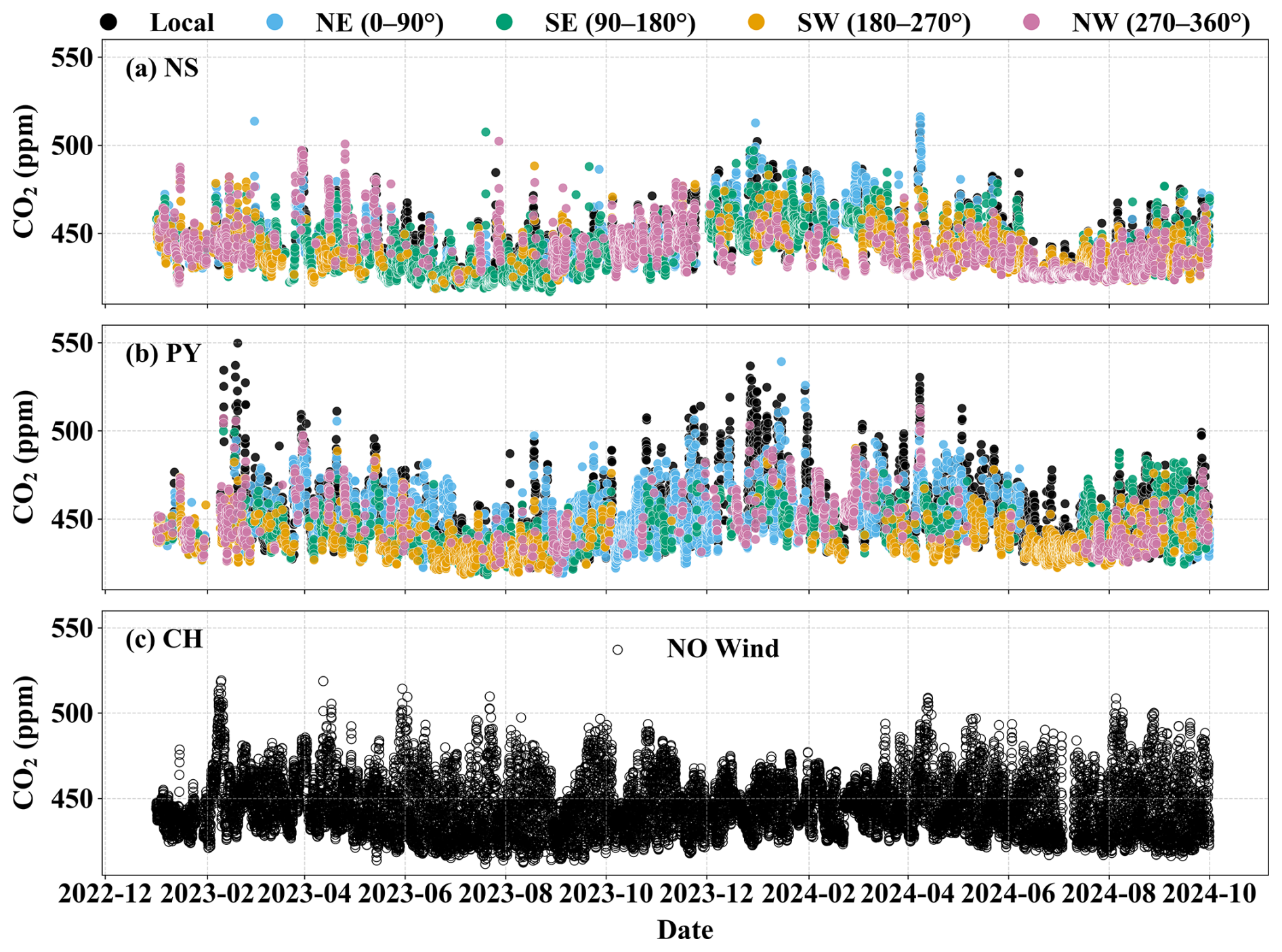
Figure 2 Time series of atmospheric CO₂ concentrations at the (a) NS, (b) PY, and (c) CH stations, points are color-coded by wind category: local conditions (wind speed < 1.5 m s⁻¹) and four directional sectors for winds ≥ 1.5 m s⁻¹ (NE, 0–90°; SE, 90–180°; SW, 180–270°; NW, 270–360°). For CH, wind-direction classification is not shown and the time series is plotted without sector coloring.

Urban–rural CO₂ gradients vary globally due to differences in economic activity, population density, land use, and energy infrastructure, reflecting heterogeneous urban carbon emissions (Gao et al., 2022). To further illustrate this spatial contrast and its seasonality, we summarized the urban–suburban/coastal gradients across the full record and report annual and seasonal means in Fig. 3. In Guangzhou, mean CO₂ concentration differences between PY and NS/CH were 6.67 and 3.43 ppm, respectively, forming a distinct “urban dome” (urban > suburban > coastal). The NS–CH difference (3.44 ppm) highlights comparable gradients between suburban and coastal zones. This gradient mirrors Los Angeles's coastal megacity profile but with a smaller magnitude (Verhulst et al., 2017). Guangzhou's urban–suburban difference (3.43 ppm) aligns with Hangzhou's 2021 observations (4.96 ppm) (Chen et al., 2024) but is lower than Nanjing (8.1 ppm, 2014) and Beijing (12.4 ppm, 2018–2019) (Gao et al., 2018; Yang et al., 2021). It remains far smaller than Shanghai (55.1 ppm, 2014) and Baltimore (66.0 ppm, 2002–2006) (Pan et al., 2016; George et al., 2007). Over time, urban emissions may stabilize as suburban populations and fossil fuel demand grow, potentially narrowing urban–suburban CO₂ differences (Mitchell et al., 2018). For instance, Hangzhou's reduced gradient reflects urbanization-driven energy consumption, where suburban monitoring captures urban emission influences (Chen et al., 2024).

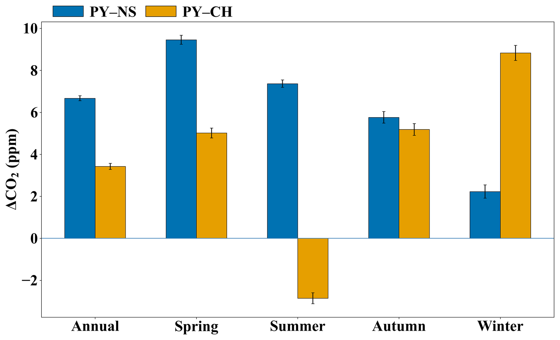
Figure 3 Urban–suburban/coastal CO₂ gradients in Guangzhou. Annual and seasonal mean concentration differences (ΔCO₂, ppm) between the urban site (PY) and the coastal site (NS) (PY–NS) and between PY and the suburban site (CH) (PY–CH). Seasons are defined as spring (March–May), summer (June–August), autumn (September–November), and winter (December–February). Error bars denote ±1 standard error (SE).

Figure 3 further shows that these spatial gradients are strongly season-dependent. PY–NS remains positive year-round but is smallest in winter (2.23 ppm), when prevailing northerlies elevate CO₂ at the coastal NS site and reduce the urban–coastal contrast, consistent with Fig. 2. PY–CH is more strongly seasonally modulated: it peaks in winter (8.83 ppm) but reverses sign in summer (−2.86 ppm), when southerly (marine-influenced) flow more frequently ventilates PY (SW/SE sectors in Fig. 2) and the CH summertime enhancement may reflect a northward-displaced urban influence plus biogenic/boundary-layer modulation (Sect. 3.1.1; Sect. 3.3). Spring and autumn show intermediate positive PY–CH (∼ 5 ppm), while PY–NS peaks in spring (9.46 ppm), consistent with enhanced coastal ventilation under southerly influence. Together, these gradients indicate a seasonally displaced CO₂ “dome” in this coastal setting, where the highest CO₂ within our network can occur outside the urban core, complementing the site-level seasonal cycles discussed in Sect. 3.1.1. This coastal, seasonally displaced CO₂ dome contrasts with patterns more commonly reported in inland megacity networks, where enhancements are typically strongest at the most urbanized sites relative to suburban/background stations (Xueref-Remy et al., 2018; Yang et al., 2021; Chen et al., 2024).

3.1.1 Seasonal variability of atmospheric CO₂

Figure 4 illustrates the monthly mean variations in atmospheric CO₂ concentrations at the NS, PY, and CH stations in Guangzhou, alongside their correlations with the Normalized Difference Vegetation Index (NDVI). NDVI data at 1 km × 1 km spatial resolution were obtained from NASA's EOSDIS Land Processes Distributed Active Archive Center (Didan, 2015), with values within a 3 km radius buffer around each station center used for comparative analysis. All three stations exhibited consistent seasonal CO₂ patterns, with higher concentrations in winter/spring and lower values in summer/autumn, mirroring observations in Hangzhou (Chen et al., 2024). These variations arise from the combined effects of (1) seasonal biogenic flux cycles, (2) anthropogenic emission variability, and (3) boundary layer height dynamics (Xueref-Remy et al., 2018). Enhanced vegetation photosynthesis during warmer months (summer/autumn, Table S3 in the Supplement) strengthens biogenic carbon sinks, while higher boundary layer depths (Fig. S6 in the Supplement) and southerly marine air masses (Fig. 2) promote atmospheric mixing and CO₂ dispersion.

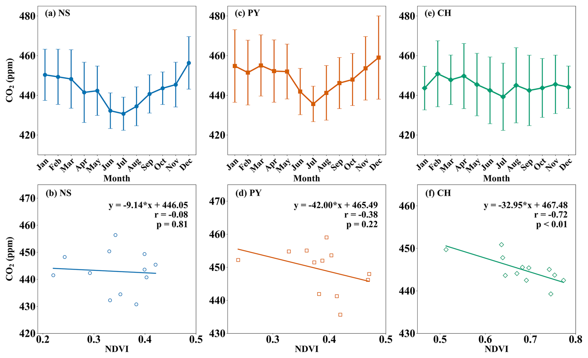
Figure 4 Monthly mean CO₂ concentrations (a, c, e) and their correlations with the Normalized Difference Vegetation Index (NDVI) (b, d, f) for the (a–b) NS, (c–d) PY, and (e–f) CH stations. Error bars indicate ±1 standard deviation (SD).

The amplitudes of the seasonal variation of CO₂ at NS, PY, and CH are 25.63, 23.38, and 11.59 ppm, respectively. NS and PY peaked in December and troughed in July, whereas CH peaked in February and troughed in July. NS's large amplitude reflects its extreme December highs and July lows. In December, prevailing northerly winds (Figs. 2a and S2a) transported urban emissions to downwind NS, narrowing its CO₂ difference with PY to 2.68 ppm. Conversely, July saw NS's CO₂ concentrations fall to the lowest among all stations – 4.93 and 8.56 ppm below PY and CH, respectively – establishing a south-to-north increasing gradient (coastal < urban < suburban). This gradient aligns with marine-influenced southerly air masses, which dilute coastal CO₂ while transporting urban emissions northward, potentially accumulating CO₂ in northern suburbs. This south–north pattern is consistent with the seasonal mean gradients in Fig. 3, which summarize how the urban–coastal contrast weakens in winter and how the urban–suburban gradient can be seasonally displaced in summer.

Although CH exhibits strong biogenic coupling (NDVI–CO₂ correlation: −0.72; Fig. 4f), NS shows an opposite seasonal contrast relative to CH (−9.80 ppm in summer; +5.80 ppm in winter), pointing to transport- and boundary-layer-driven variability at the coastal site. At NS, the NDVI–CO₂ correlation is weak (−0.08) and NDVI varies within a narrow range (0.22–0.42), indicating limited local biogenic control, whereas seasonal shifts in marine–continental transport (summer dilution vs. winter urban outflow) and boundary-layer depth jointly modulate dilution and accumulation (Figs. 2 and S6). In February, CH recorded its annual CO₂ maximum, driven by vegetation respiration during early growth stages and elevated emissions from fireworks around the Lunar New Year, as CH's location falls outside Guangzhou's fireworks restriction zones (https://www.gz.gov.cn/gfxwj/qjgfxwj/chq/qf/content/post_7198980.html, last access: 18 June 2025). This interpretation is supported by CO, a tracer for combustion-derived CO₂ (Newman et al., 2013; Che et al., 2022a): CH's CO concentrations also peaked in February due to firework emissions, whereas other sites peaked in December (Fig. S7 in the Supplement).

3.1.2 Diurnal variations of atmospheric CO₂

The diurnal patterns of atmospheric CO₂ concentrations at NS, PY, and CH stations in Guangzhou consistently exhibited lower daytime and higher nighttime values (Fig. 5). This is attributed to the shallow nocturnal boundary layer, which traps anthropogenic and biogenic fluxes near the surface, elevating CO₂ levels. After sunrise, surface heating deepens the boundary layer, diluting surface emissions and entraining free tropospheric air with lower CO₂ concentrations. Concurrently, daytime photosynthetic uptake further reduces near-surface CO₂ (Mitchell et al., 2018). We further evaluate urban–suburban–coastal differences in these processes. At PY, the CO₂ peak occurred at 08:00–09:00 LT, aligning with morning traffic peaks, reflecting dominant anthropogenic influences. CH's peak appeared 1–2 h earlier than PY due to its longitudinal and elevational position, where earlier sunrise accelerates the breakup of the nocturnal stable boundary layer. Both PY and CH reached minima at 16:00–17:00 LT, likely linked to afternoon photosynthetic activity. NS exhibited irregular peak/valley timing.

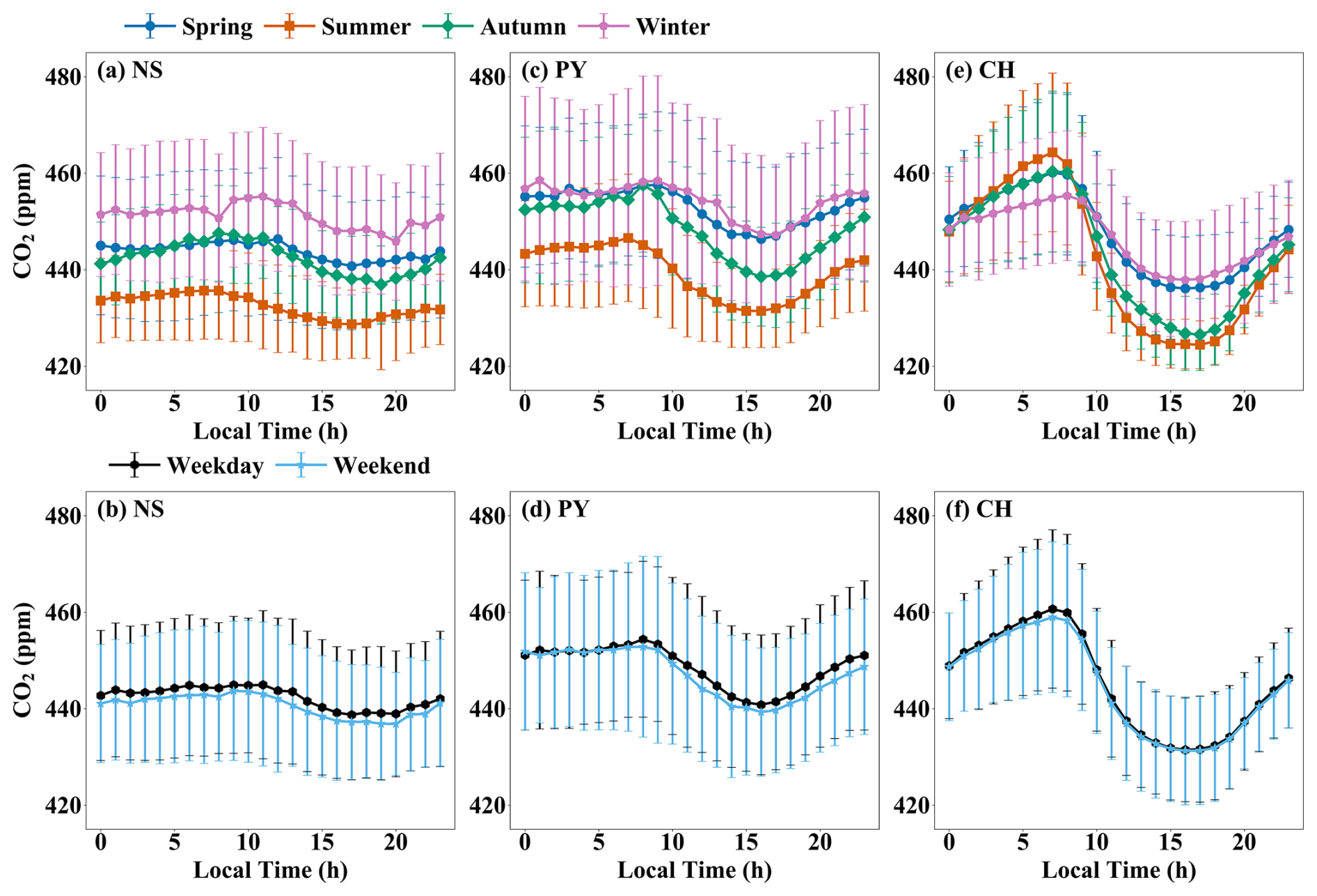
Figure 5 Diurnal CO₂ variations at the (a–b) NS, (c–d) PY, and (e–f) CH stations, shown across seasons (a, c, e) and weekdays/weekends (b, d, f). Seasons are defined as spring (March–May), summer (June–August), autumn (September–November), and winter (December–February). Error bars indicate ±1 SD. The corresponding CO diurnal cycles are shown in Fig. S9.

Diurnal amplitudes at CH and PY were larger in summer/autumn than winter/spring, driven by vegetation activity and boundary layer dynamics (Fig. S8 in the Supplement). Summer/autumn conditions in Guangzhou – abundant light, warmth, and rainfall – optimize vegetation growth, enhancing daytime photosynthesis and nighttime respiration (Dusenge et al., 2019). Optimal canopy temperatures for subtropical evergreen forests (∼ 30 °C) (Liu et al., 2015) align with CH/PY's summer/autumn daytime temperatures (Table S3), explaining their amplified amplitudes. However, the diurnal amplitude of CO₂ at CH in summer and autumn is 2.63 times and 1.77 times that at PY, respectively. The diurnal amplitude of atmospheric CO₂ concentration at CH in summer is 39.90 ppm, which is close to the diurnal amplitude of CO₂ concentration in the suburbs of Hangzhou in summer (35.29 ppm) (Chen et al., 2024). Despite similar temperatures, CH's larger NDVI range and stronger NDVI–CO₂ correlation (−0.72 vs. PY; Fig. 4d and f) highlight greater biogenic dominance, with pronounced daytime uptake and nighttime respiration. NS showed the smallest diurnal amplitudes across seasons (e.g., 5.60 ppm in summer), attributable to sparse vegetation (low NDVI: 0.22–0.42) and frequent summer southerly marine air masses, which dilute coastal CO₂.

Figure 5 contrasts weekday–weekend diurnal CO₂ patterns. All stations generally showed higher weekday concentrations, diverging from Hangzhou and Beijing (Yang et al., 2021; Chen et al., 2024) but aligning with Paris and Boston (Briber et al., 2013; Xueref-Remy et al., 2018). At CH, the daytime weekday–weekend contrast is small. This could reflect a weak anthropogenic weekday–weekend signal relative to other sources of variability, but it does not uniquely diagnose source dominance because transport and boundary-layer mixing may dilute or mask weekday–weekend differences. At PY, the clearer daytime weekend decrease is consistent with reduced on-road activity in the urban core. At NS, weekday CO₂ remains higher across much of the day, which may reflect weekday-intensified construction and port-related logistics in the surrounding area (for example, the Metro Line 18 extension and operations near the Nansha Container Terminal Phase III, ∼ 5 km east), superimposed on transport and mixing effects.

To corroborate the combustion contribution to the CO₂ diurnal cycle, we examined synchronous CO measurements (Fig. S9 in the Supplement). At all sites, CO shows a consistent seasonal ordering (winter highest, summer lowest), and its morning maximum at PY (typically 08:00–10:00 LT) coincides with the CO₂ morning peak (Fig. 5), supporting traffic/combustion control of the early-day enhancement. In contrast to CO₂, CO exhibits only a weak mid-afternoon minimum (including at CH), consistent with CO₂ being additionally depressed by photosynthetic uptake while CO is unaffected; both species remain modulated by transport and boundary-layer mixing. Weekday–weekend differences are small at CH but clearer at PY/NS (Fig. S9), indicating a stronger anthropogenic weekly-cycle imprint in the urban-core and coastal/port settings. Overall, the CO–CO₂ contrast reinforces our interpretation that the morning CO₂ maxima are primarily combustion-driven, whereas the pronounced mid-afternoon CO₂ minima at vegetated sites reflect biogenic uptake rather than reduced emissions.

3.2 Sea–land breeze impacts

Based on meteorological observations from the NS coastal tall tower, 84 sea–land breeze days (SLBD) were identified in Guangzhou between January 2023 and September 2024, accounting for 13.14 % of the monitoring period, with peaks in spring and autumn. These transitional seasons between summer and winter are characterized by weaker synoptic systems and lighter background winds, favoring SLBD occurrence (Mai et al., 2024b). Our results align with SLBD seasonal distributions for the Pearl River Estuary cities of Zhuhai and Guangzhou in 2022 (Zhang et al., 2024; Mai et al., 2024b). Figure 6 compares CO₂ concentrations during SLBD and non-SLB days (NSLBD) across stations. Overall, average CO₂ concentrations during SLBD were lower than during NSLBD by 5.87 ppm at NS, 3.08 ppm at PY, and 0.75 ppm at CH. This indicates that SLB circulation enhances ventilation and CO₂ dispersion, with the SLBD-related reduction decreasing from the coastal site to the urban core and being smallest at the suburban site (NS > PY > CH). This pattern is similar to SLB-driven dispersion reported for PM_2.5, PM₁₀, and ozone in Tianjin (Hao et al., 2017). Seasonal differences were pronounced: SLB promoted CO₂ dispersion at NS and PY in spring, winter, and autumn (spring > winter > autumn), but increased CO₂ accumulation in summer. Tianjin similarly observed summer PM_2.5 $/$ PM₁₀ accumulation under SLB (Hao et al., 2017). At CH, SLBD reduced CO₂ in spring, summer, and autumn but increased it in winter, likely due to limited inland SLB penetration and competing winter processes.

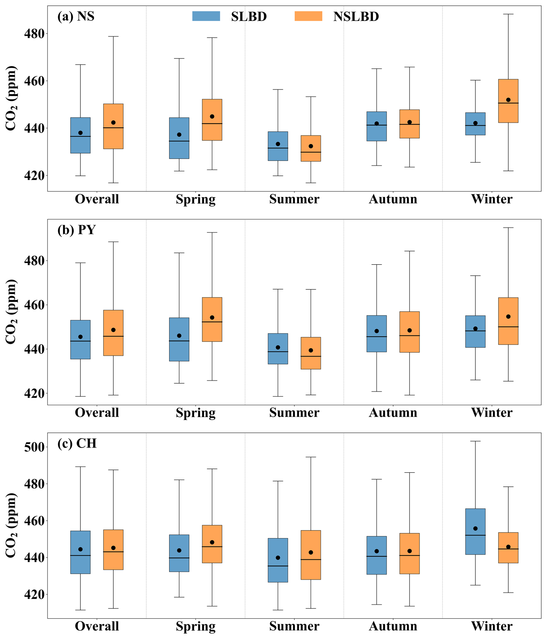
Figure 6 Boxplots of atmospheric CO₂ concentrations (black dots denote means; black lines denote medians) during sea–land breeze days (SLBD) and non-SLB days (NSLBD) across seasons (including overall) for the (a) NS, (b) PY, and (c) CH stations, with outliers excluded.

To resolve seasonal and diurnal SLB impacts, we analyzed CO₂ diurnal variations during SLBD and NSLBD (Fig. 7). Focusing on NS (due to similar PY–NS trends and space constraints), spring and winter SLBD reduced CO₂ concentrations by 7.76 and 9.77 ppm (hourly mean differences), respectively, driven by stronger winds (Fig. 7) and deeper boundary layers (Fig. S10 in the Supplement). Autumn SLB only reduced CO₂ during sea breeze hours (mean difference: 1.69 ppm). Autumn's weaker winds and boundary layers resulted in reduced dispersion compared to spring/winter. In summer, SLB increased CO₂ by 2.08 ppm (sea breeze hours) due to stable atmospheric stratification. Summer temperatures were 6.00 and 12.19 °C higher than spring and winter (Table S3), respectively. Under calm, rain-free conditions, the collision of moist marine air with dry-hot coastal land formed a thermal internal boundary layer (TIBL), inducing low-level temperature inversions near the SLB convergence zone (Liu et al., 2001; Reddy et al., 2021). These inversions suppressed horizontal/vertical mixing, trapping CO₂ (Stauffer et al., 2015; Hao et al., 2024). NS's summer SLBD winds averaged 1.05 m s⁻¹ (sea breeze) and 0.96 m s⁻¹ (land breeze) – 38.60 %, 63.16 %, and 15.32 % lower than spring, winter, and autumn winds, respectively – while boundary layer heights (590.54 m) were 9.51 % shallower than NSLBD (Fig. S10). Weak winds and shallow boundary layers stabilized atmospheric stratification, limiting CO₂ dispersion and elevating ground-level CO₂ by up to 4.03 ppm.

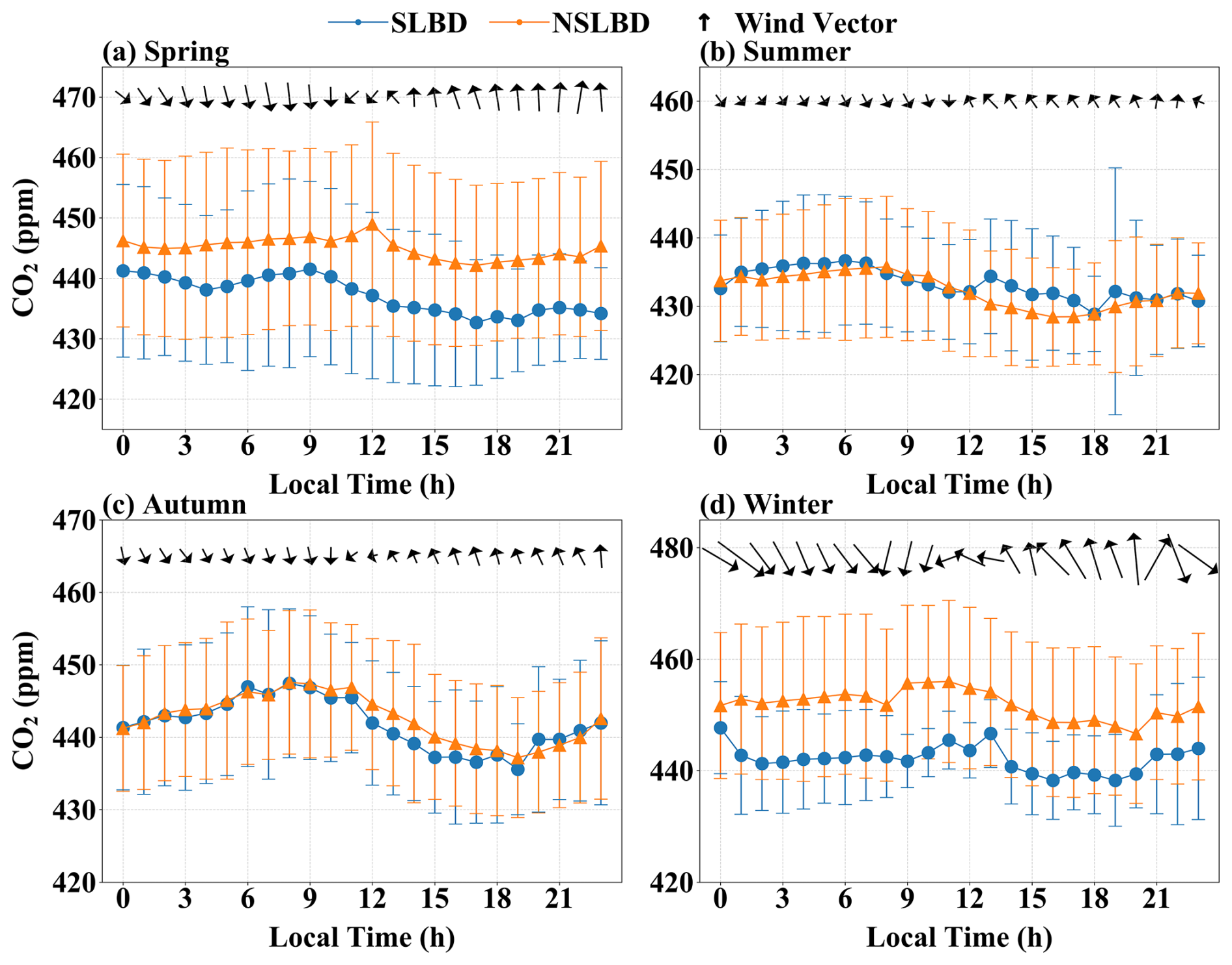
Figure 7 Diurnal variations in CO₂ concentrations, wind direction, and wind speed at the coastal station (NS) during sea–land breeze days (SLBD) and non-SLB days (NSLBD) for (a) spring (March–May), (b) summer (June–August), (c) autumn (September–November), and (d) winter (December–February). Error bars indicate ±1 SD. The corresponding CO diurnal cycles are shown in Fig. S11.

CO provides a combustion-specific tracer to further diagnose SLB modulation of anthropogenic signals (Fig. S11 in the Supplement). In spring and winter, CO is generally lower on SLBD than on NSLBD, consistent with enhanced dilution and export by the breeze circulation, broadly mirroring the CO₂ behavior (Fig. 7). In autumn, the CO response is weaker and transitional, with only modest daytime reductions. In summer, however, SLB days exhibit a pronounced afternoon CO build-up, with a much larger relative enhancement than CO₂ (relative to the seasonal 24 h mean on NSLBD: ∼ 10 % for CO versus ∼ 0.7 % for CO₂), implying trapping/recirculation of fresh combustion plumes under weak-wind, shallow-mixing conditions. Overall, the joint CO–CO₂ behavior confirms that SLB exerts a seasonally varying control on near-surface carbon signals – ventilating in cooler seasons but favoring accumulation under the stagnant summer regime.

3.3 CO₂ enhancements and uncertainties

Figure S12 (in the Supplement) presents the time series of observed CO₂ and CO concentrations at Guangzhou's stations relative to marine backgrounds from 1 January to 27 December 2023. Compared to urban observations with significant hourly variability, marine background concentrations in Guangzhou remained stable, with summer and winter CO₂ standard deviations of 0.94 and 0.67 ppm, respectively, indicating minimal local source/sink influences. Using Eqs. (13) and (14), marine background uncertainties were calculated (Table S4 in the Supplement). Summer and winter CO₂ marine background uncertainties were 0.96 and 0.70 ppm, respectively, constraining urban marine background uncertainties below 1 ppm – slightly lower than Los Angeles's 1.4 ppm (Verhulst et al., 2017). CO marine background uncertainties were 12.68 ppb (summer) and 18.36 ppb (winter).

Based on background concentrations, CO₂ enhancements were derived for all stations. Figure 8 shows enhancements across all hours, afternoon (12:00–16:00 LT), and midnight (00:00–05:00 LT) periods in 2023, summer, and winter. Annual median enhancements were 13.59 (NS), 17.70 (PY), and 16.29 ppm (CH), with pronounced spatiotemporal variability – closely aligning with the 10–20 ppm range observed annually in the Beijing–Tianjin–Hebei (BTH) urban cluster of China (Han et al., 2024). In summer, the all-hours enhancement followed a south-to-north gradient: 7.00 (NS), 13.23 (PY), and 16.91 ppm (CH). This inland maximum likely reflects the combined influence of coastal transport, biogenic exchange, and boundary-layer mixing, and is consistent with the seasonal gradient displacement discussed in Sect. 3.1 (Fig. 3). Afternoon enhancements peaked at PY (6.92 ppm), whereas midnight enhancements at CH reached 31.36 ppm. Winter afternoon enhancements reversed this pattern: 16.58 (NS), 12.37 (PY), and 7.45 ppm (CH), with NS and PY values 4.39 times and 1.79 times higher than summer. Midnight enhancements at CH remained highest in winter (18.87 ppm), despite a 38.93 % reduction from summer.

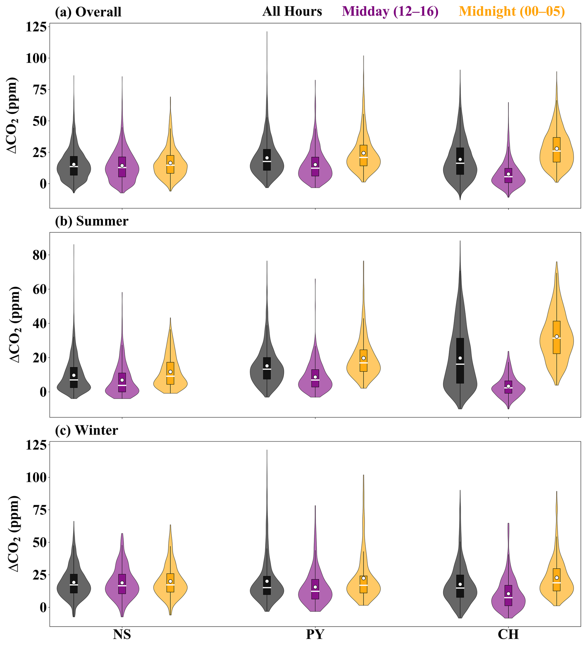
Figure 8 Distributions of hourly CO₂ enhancement (ΔCO₂) above the background concentrations at NS, PY, and CH during the (a) overall, (b) summer, and (c) winter periods, shown for all hours, midday (12:00–16:00 LT), and midnight (00:00–05:00 LT). White dots denote the mean values, and white horizontal lines denote the median values.

This spatiotemporal variability reflects divergent influences of anthropogenic emissions, biogenic fluxes, and atmospheric mixing. At CH, strong diurnal shifts in enhancements (e.g., 31.36 ppm summer midnight) highlight biogenic dominance, with long-tailed distributions (Fig. 8). Stable, shallow nighttime boundary layers trapped respiratory emissions near the surface, consistent with isotopic studies in Xi'an (32.80 ppm) and Switzerland (30.00 ppm) (Wang et al., 2021; Berhanu et al., 2017). At NS, transport dominated: summer southerly marine air masses reduced enhancements, while winter northerly winds transported urban emissions downstream, raising NS enhancements to PY levels (exceeding PY in afternoons). PY's enhancements were primarily anthropogenic, validated by CO co-variation. CO, a tracer for combustion-derived CO₂, showed significantly higher concentrations at PY (Fig. S12). PY's median midnight CO enhancements in summer were 2.04 times and 1.43 times higher than NS and CH (Fig. S13 in the Supplement). Shallow nocturnal boundary layers localized anthropogenic CO near the surface, with minimal vertical/horizontal transport, confirming PY's anthropogenic dominance.

3.4 Continuous observations of ΔCO $/$ ΔCO₂ ratios

Reduced Major Axis regression (Model II) was applied to analyze the relationship between CO (ΔCO) and CO₂ (ΔCO₂) concentration enhancements across stations, with the ΔCO $/$ ΔCO₂ emission ratio (R_CO) derived from regression slopes (Fig. 9). In 2023, R_CO values for NS, PY, and CH were 8.48 ± 1.81, 7.45 ± 1.38, and 4.16 ± 3.59 ppb ppm⁻¹, respectively, with correlation coefficients of 0.78, 0.72, and 0.33, indicating significant spatiotemporal heterogeneity. Summer R_CO was generally lower than winter, with CH exhibiting the lowest seasonal value (2.66 ± 0.83 ppb ppm⁻¹). Winter maxima occurred at NS (11.03 ± 1.49 ppb ppm⁻¹), followed by PY (9.08 ± 1.13 ppb ppm⁻¹) and CH (8.56 ± 1.82 ppb ppm⁻¹).

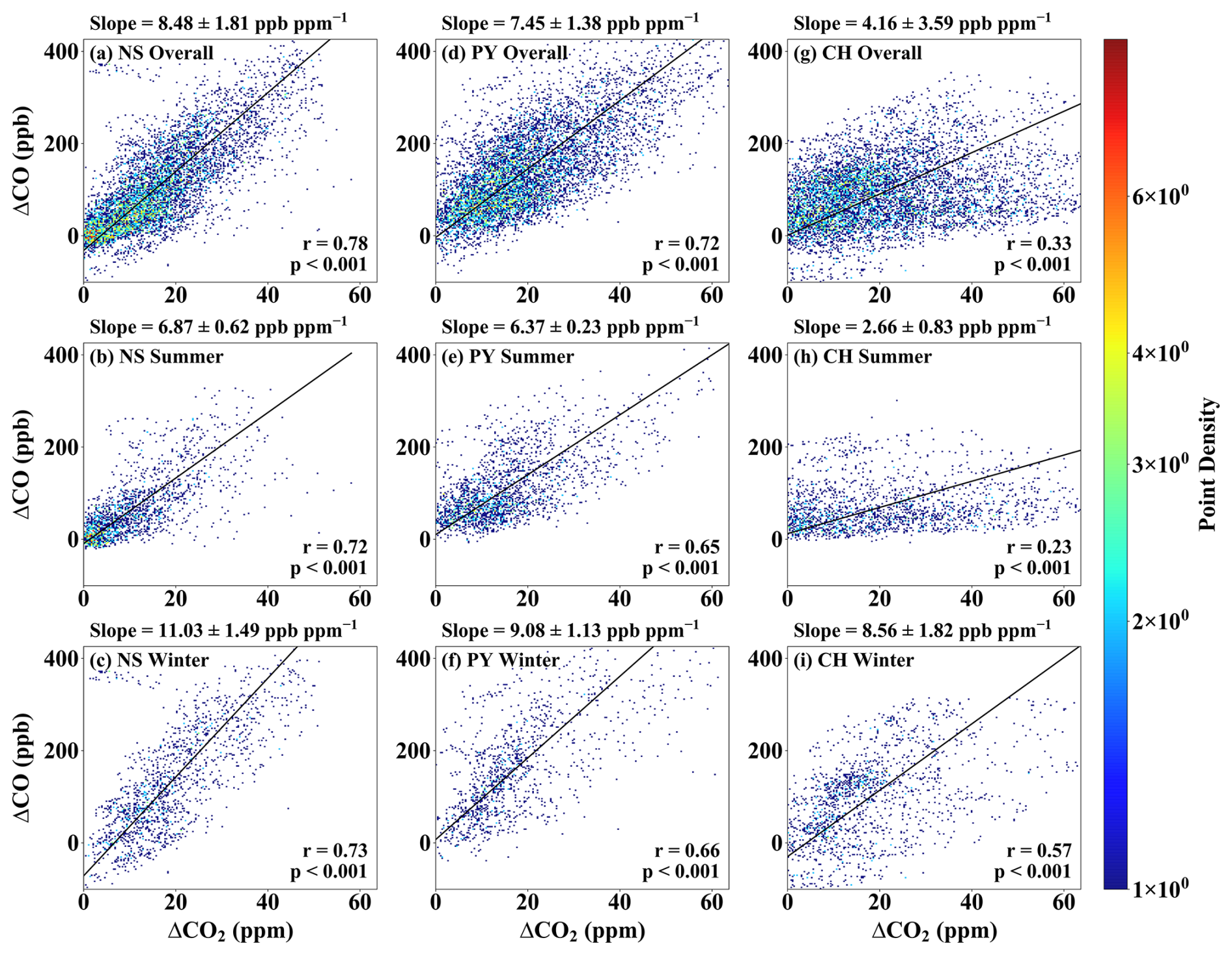
Figure 9 Seasonal relationships between ΔCO₂ and ΔCO enhancements at the (a–c) NS, (d–f) PY, and (g–i) CH stations, analyzed using geometric-mean regression. Panels are shown as two-dimensional (2-D) histogram density plots (hist2d; 200 × 200 bins), where color indicates the number of paired observations per bin. The fitted slope represents the ΔCO $/$ ΔCO₂ emission ratio (R_CO; ppb ppm⁻¹), reported as mean ±1 SD (reflecting temporal variability).

Comparatively, Beijing's urban R_CO in 2019 was measured at 10.46 ± 0.11 ppb ppm⁻¹ using portable Fourier-transform spectroscopy (Che et al., 2022a), while Shanghai and Los Angeles showed 10.22 ± 0.40 and 9.64 ± 0.46 ppb ppm⁻¹, respectively, based on satellite and model data (Wu et al., 2022a). Guangzhou's lower R_CO is consistent with the post-2013 tightening of China's air-quality management across the energy and transport sectors, rather than a single intervention. National action plans (2013–2017 Air Pollution Prevention and Control Action Plan; 2018–2020 Three-Year “Blue-Sky” Action Plan) strengthened coal/industrial and vehicle-emission controls with explicit targets and timelines. In parallel, ultra-low-emission (ULE) retrofits of coal-fired power units were rolled out through 2020, and China 6 (VI) on-road emission standards were phased in, with large cities (including Guangzhou) leading implementation; Guangdong's provincial Blue-Sky measures further reinforced industrial/mobile-source controls and promoted fleet electrification. These measures coincide with independent inventory evidence of declining national CO emissions (∼ 23 % during 2013–2017) (Zheng et al., 2018), plausibly reducing CO $/$ CO₂ emission ratios from dominant urban sources. Consistently, Beijing's R_CO decreased from > 30 ppb ppm⁻¹ in 2006 (Han et al., 2009) to 10.22 ± 0.40 ppb ppm⁻¹ by 2020 (Wu et al., 2022a), with additional reductions during the 2008 Olympics and 2020 COVID-19 lockdowns (Wang et al., 2010; Cai et al., 2021). In Guangdong, restrictions on coal plants, retirement of inefficient industries, and promotion of electric vehicles coincided with large declines in SO₂ and NO₂ (85 % and 35 % in 2019 relative to 2006) (Hu et al., 2021), and Mai et al. (2021) likewise reported improved combustion efficiency in the PRD associated with advances in gasoline vehicles. We emphasize that this interpretation is consistency-based rather than a formal causal identification; fuel mix, fleet composition, and atmospheric oxidation may also contribute (Young et al., 2023; Vimont et al., 2019).

Seasonal R_CO variations stem from biogenic exchange and transport dynamics. Summer's weaker ΔCO–ΔCO₂ correlations at CH reflect dominant biogenic influences (daytime uptake and nighttime respiration), as reported in Beijing, Indianapolis, and Switzerland (Turnbull et al., 2015; Berhanu et al., 2017; Che et al., 2022a). Biogenic impacts decreased from suburban > urban > coastal, aligning with vegetation gradients. Winter's higher R_CO at CH and NS correlated with reduced biogenic activity and northerly transport of urban emissions under stable boundary layers. Berhanu et al. (2017) attributed winter R_CO increases to cold-air advection and boundary layer accumulation. NS's winter R_CO (4.16 ppb ppm⁻¹ higher than summer) linked to urban airmass origins, while PY's seasonal shifts reflected suburban source–sink variations. Although secondary CO from upwind Volatile Organic Compounds (VOCs) and Methane (CH₄) oxidation could perturb R_CO, their combined contribution was merely 1 % in coastal urban regions (Griffin et al., 2007).

3.5 Partitioning anthropogenic and biogenic fluxes

Section 3.4 shows that the sites differ in how well the ΔCO–ΔCO₂ relationship reflects fossil-fuel combustion. At CH, especially in summer, CO₂ variability is strongly influenced by biogenic exchange, which weakens the combustion linkage implied by R_CO and can bias an R_CO-based fossil-fuel estimate. At NS, in contrast, variability is dominated by changing transport and upwind airmass origin, particularly in winter when urban plumes frequently reach the coastal site. We therefore select PY – the urban-core site with a comparatively robust combustion signal – to quantify the surface CO₂ emissions (CO₂tot) constrained by the observed concentration enhancements and footprint-informed transport. Using the PY-specific R_CO, we then partition CO₂tot into fossil-fuel (CO₂ff) and biogenic (CO₂bio) components.

Figure 10 summarizes mean afternoon (12:00–16:00 LT) CO₂tot, CO₂ff, and CO₂bio at PY for July 2023 (summer) and December 2023 (winter). Bars show monthly means of daily afternoon values. The plotted error bars indicate ±1 standard deviation (SD) across days and thus represent day-to-day variability in ventilation, mixing, and transport rather than uncertainty of the monthly mean. Mean uncertainty is quantified by the standard error (SE), which is distinct from the SD shown in Fig. 10. In July, CO₂tot = 2.38 ± 0.45, CO₂ff = 5.97 ± 0.75, and CO₂bio = −3.59 ± 0.63 µmol m⁻² s⁻¹ (mean ± SE), whereas in December CO₂tot = 13.50 ± 2.20, CO₂ff = 13.56 ± 2.40, and CO₂bio = −0.06 ± 1.13 µmol m⁻² s⁻¹ (Table S5). Because CO₂bio is diagnosed as a residual (CO₂bio = CO₂tot − CO₂ff), its uncertainty reflects propagated uncertainties from both CO₂tot and CO₂ff – including measurement and background-selection uncertainty and R_CO-related variability – rather than being independent. Notably, December CO₂bio is close to zero. The bootstrap 95 % CI of the monthly mean is [−2.28, 2.09] µmol m⁻² s⁻¹, which includes zero, indicating that the net biogenic flux was not statistically distinguishable from zero during winter afternoons, likely reflecting a near-neutral balance between photosynthesis and respiration. In contrast, the July mean CO₂bio remains clearly negative relative to its uncertainty, supporting robust summertime net biogenic uptake despite uncertainty propagation inherent to the residual calculation. When assessed using daily afternoon means, the July–December contrasts are statistically significant for CO₂tot, CO₂ff, and CO₂bio (Welch and Mann–Whitney tests; bootstrap 95 % confidence intervals; Table S5). Robust distributional metrics corroborate this significant seasonal increase despite partial day-to-day overlap: the CO₂ff median increases from 4.33 (IQR: 3.58–7.81) in July to 10.70 (IQR: 6.74–18.28) µmol m⁻² s⁻¹ in December. Across both months, CO₂ff is larger in magnitude than CO₂bio, implying that the PY afternoon enhancement is primarily fossil-fuel driven, consistent with fossil-dominated urban enhancements reported for other Chinese cities (Wang et al., 2022). The stronger winter CO₂ff relative to summer is explained mainly by atmospheric dynamics – reduced dilution under weaker marine ventilation and a shallower boundary layer – while seasonal emission changes (e.g., winter residential energy use) likely provide a secondary contribution. In contrast, CO₂bio is more negative in summer, consistent with higher summer NDVI (+11 %) and warmer conditions approaching optimal canopy temperatures (Table S3).

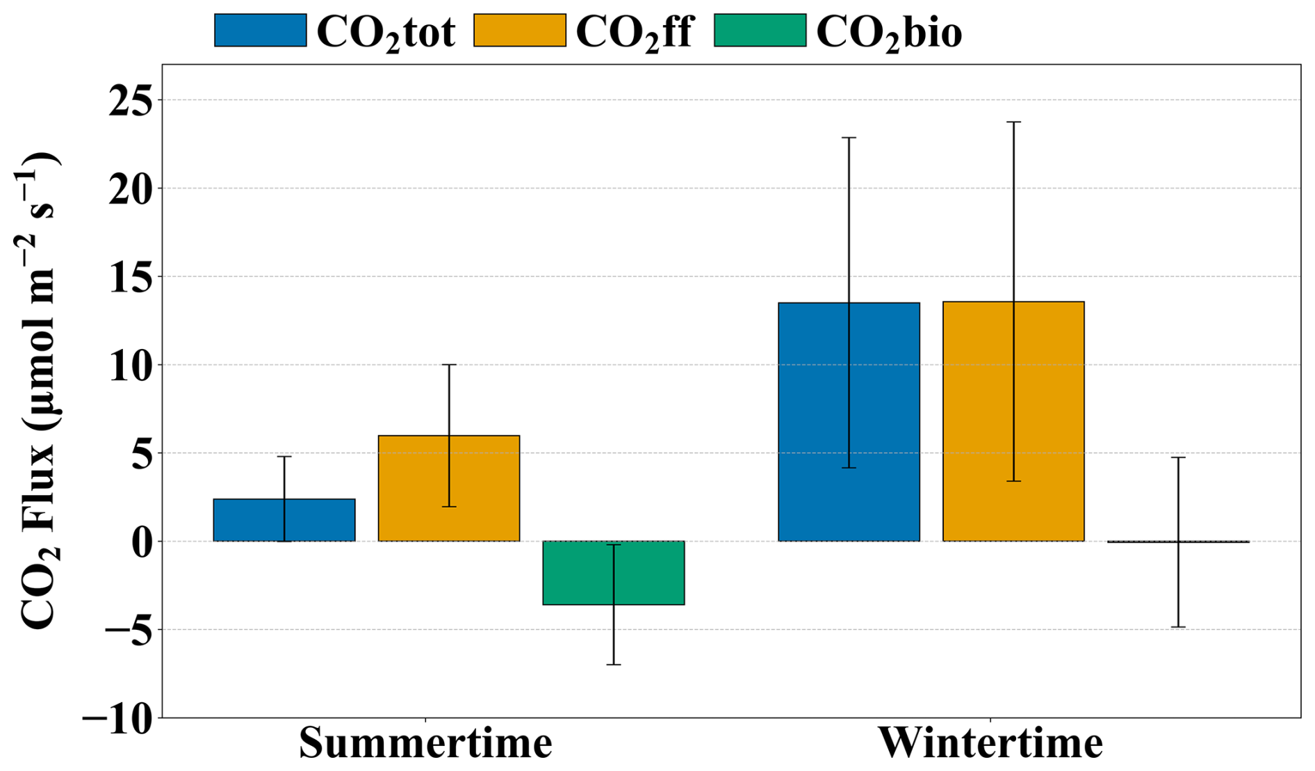
Figure 10 Average afternoon (12:00–16:00 LT) CO₂tot, CO₂ff, and CO₂bio at PY for July 2023 (summer; n = 29 valid days) and December 2023 (winter; n = 18 valid days). December has fewer valid days because objective QC excluded days with incomplete afternoon coverage (e.g., instrument downtime/maintenance), so the smaller winter sample reflects data availability rather than subjective selection. Bars show monthly means of daily afternoon values. Error bars indicate ±1 SD across daily afternoon means within each month (day-to-day atmospheric variability), not the SE of the monthly mean; SE and confidence intervals are reported in Table S5.

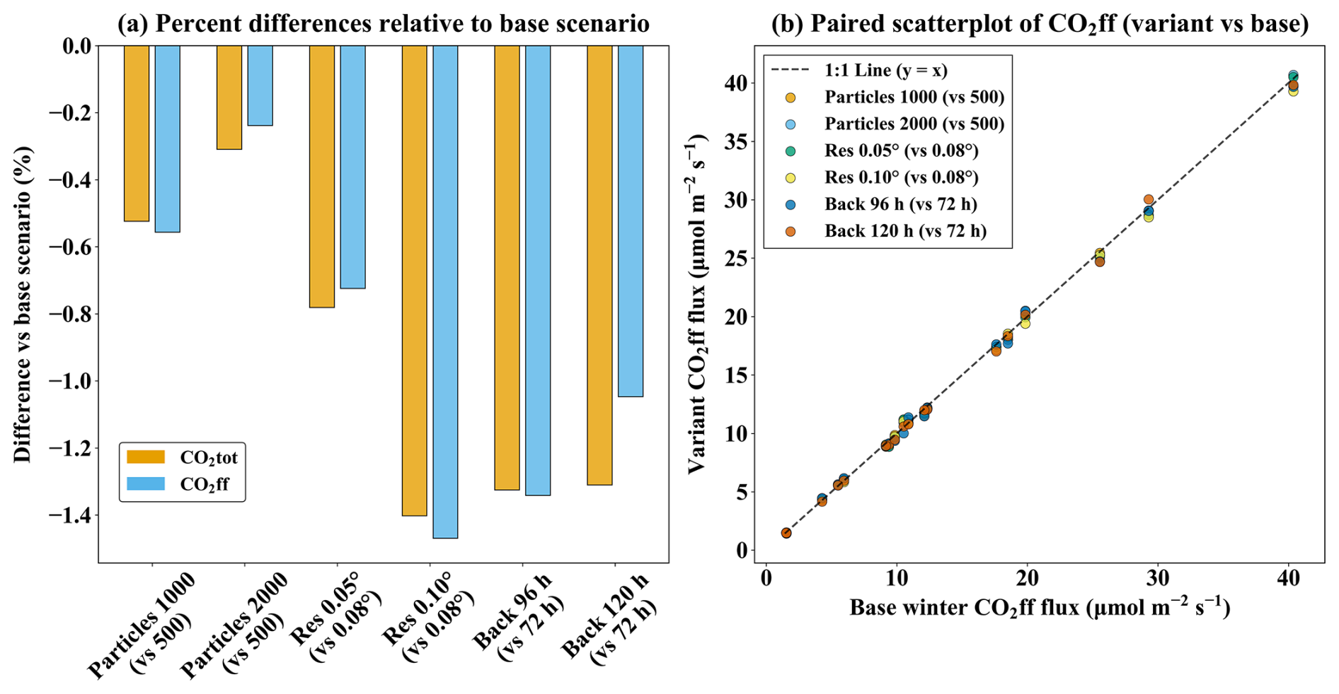
Figure 11 STILT parameter sensitivity at PY (winter). (a) Mean percent difference (variant − baseline) of inferred fluxes relative to the winter baseline (500 particles, 0.08°, 72 h), computed from paired daily afternoon means (12:00–16:00 LT; n = 18); Δ% = (variant − base) $/$ base × 100; negative values indicate lower than baseline. (b) Paired scatter of CO₂ff (µmol m⁻² s⁻¹) from each variant versus the baseline for the same days; solid line is 1 : 1 (y = x).

To test the robustness of the winter fossil-fuel dominance inferred at PY – when combustion signals are strongest – we reran the winter flux-estimation workflow using paired daily afternoon means (12:00–16:00 LT). We then varied (1) particle number (1000/2000), (2) grid spacing (0.05/0.10°), and (3) backward duration (96/120 h) relative to the baseline (500 particles, 0.08°, 72 h). Mean changes were small for both components (Table S6 in the Supplement; Fig. 11a). Increasing particle number to 1000/2000 changed CO₂ff by −0.56 %/−0.24 % and CO₂tot by −0.52 %/−0.31 %. Refining the grid to 0.05° yielded comparably small decreases (CO₂ff: −0.72 %; CO₂tot: −0.78 %). Extending the backward duration to 96/120 h produced changes of −1.34 %/−1.05 % for CO₂ff and −1.33 %/−1.31 % for CO₂tot. Only the coarser 0.10° grid produced a statistically detectable, yet small, decrease (CO₂ff: −1.47 %, p = 0.0269; CO₂tot: −1.40 %, p = 0.0164). All other settings yielded changes ≤ 1.34 % with 95 % CIs spanning zero (p ≥ 0.083), indicating no evidence of material bias at our sample size. Day-to-day consistency remained essentially unchanged across settings, with extremely high correlations (CO₂ff: r = 0.9993–0.9997; CO₂tot: r = 0.9992–0.9997) and small RMSE values (CO₂ff: 0.31–0.45 µmol m⁻² s⁻¹; CO₂tot: 0.28–0.45 µmol m⁻² s⁻¹), consistent with the near-1 : 1 paired scatter (Fig. 11b). Because wintertime CO₂bio at PY was close to zero, percent differences were not informative; in absolute terms, test–baseline differences in CO₂bio remained small (order 10⁻² µmol m⁻² s⁻¹) with 95 % CIs generally spanning zero, consistent with the tight across-run daily spread (median 0.045 µmol m⁻² s⁻¹; IQR 0.016–0.067 µmol m⁻² s⁻¹) (Table S7 in the Supplement). Across the baseline plus six variants, the day-by-day ensemble spread was tightly bounded (median 0.20–0.21 µmol m⁻² s⁻¹, median CV ≈ 1.8 %). Together, these results indicate that our baseline STILT configuration lies in a converged regime and that the inferred winter CO₂ff dominance is robust to reasonable transport-parameter choices.

For winter afternoons at PY, measurement and background-selection uncertainties – estimated by propagating their combined enhancement uncertainty through Eqs. (12)–(14) – contribute only ∼ 0.36 µmol m⁻² s⁻¹, i.e., ∼ 3 % of the mean winter-afternoon CO₂ff. Paired-day STILT sensitivity tests (Fig. 11) further indicate that the winter-afternoon CO₂ff attribution is robust to reasonable transport-parameter choices. The remaining uncertainty is thus more likely dominated by residual transport representation error and coastal mesoscale flow (e.g., wind and boundary-layer mixing biases), as documented for winter conditions in meteorological/transport modeling (Yadav et al., 2021; Lin et al., 2021). To provide independent context, we benchmark our winter-afternoon estimate against bottom-up inventories, which are used solely for contextual comparison and do not enter the CO₂ partitioning. We use 2023 inventories at 0.1° × 0.1° resolution, temporally disaggregate annual totals to hourly emissions using the same profiles (Crippa et al., 2020), and compute the winter-afternoon (12:00–16:00 LT) mean emission flux over the winter footprint-defined sensitivity region (Fig. 12). This yields 19.81 µmol m⁻² s⁻¹ from the EDGAR_2024_GHG (2023) inventory (Crippa et al., 2024) and 85.46 µmol m⁻² s⁻¹ from the MEIC-global-CO₂ (2023) inventory (Xu et al., 2024). While this aligns qualitatively with higher MEIC estimates reported for Guangdong Province (Yang et al., 2025), the contrast is larger for our winter-afternoon sensitivity region. This likely reflects differences in spatial disaggregation and point-source representation (e.g., road-network allocation and power-plant locations) that can be accentuated at sub-provincial scales (Yang et al., 2025).

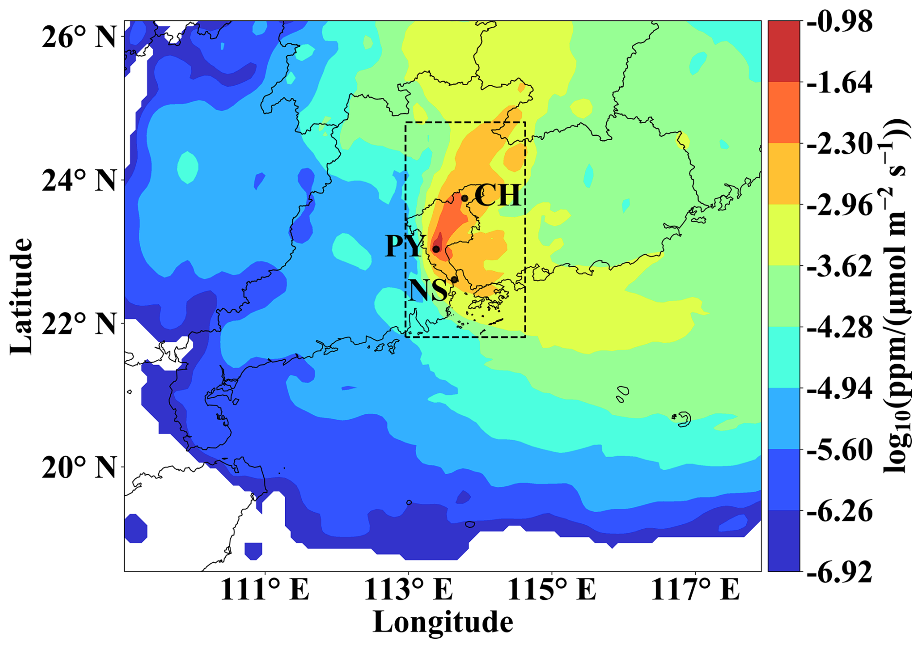
Figure 12 Spatial distribution of the mean winter-afternoon (12:00–16:00 LT) STILT footprint at the PY station, representing the receptor sensitivity to upwind surface fluxes. Colors denote the log10-transformed footprint sensitivity (ppm (µmol m⁻² s⁻¹)⁻¹). The dashed rectangle outlines the sensitivity region used for inventory flux aggregation and benchmarking in Sect. 3.5.

Notably, our observation-based CO₂ff reflects the footprint-weighted enhancement sampled at PY during winter afternoons after background removal, whereas inventories provide gridded emission fields from which an unweighted domain-mean afternoon flux can be computed over the sensitivity region. Because only grid cells with substantial STILT footprint influence contribute materially to the receptor enhancement – and these weights are highly heterogeneous and transport-dependent (Fig. 12) – the unweighted domain-mean inventory flux may be non-uniformly represented in the receptor signal under variable coastal transport (Gerbig et al., 2003; Lin et al., 2003; Fasoli et al., 2018). Accordingly, an effective footprint-weighted mean flux estimate inferred from the receptor enhancement can differ from the unweighted afternoon-mean inventory flux over the sensitivity region. This difference depends on the spatial alignment between heterogeneous transport footprints and spatially heterogeneous emissions (including localized hotspots), because under a given transport regime many grid cells within the domain may carry negligible footprint influence (Hüser et al., 2017; Kunik et al., 2019). We therefore interpret inventory comparisons as a plausibility envelope that reflects inter-inventory spread, rather than a validation target. Such inventory–observation differences are also reported for other coastal urban basins (e.g., Los Angeles) and are often sensitive to boundary-layer representation and meteorological inputs (Kim et al., 2025).

Beyond the winter fossil-fuel benchmark above, we further place the summer biogenic component and its offset ratio in the context of independent regional and urban estimates. Summer afternoons exhibited mean CO₂bio of −3.59 ± 0.63 µmol m⁻² s⁻¹, consistent with observation-based Pearl River Delta NEE (−0.1 to −12 µmol m⁻² s⁻¹) (Mai et al., 2024a), and with modeled urban biogenic flux ranges (0 to −15 µmol m⁻² s⁻¹) reported in previous studies (Wu et al., 2021; Wei et al., 2022; Kim et al., 2025). Consequently, summer-afternoon biogenic uptake offsets 60.13 % of concurrent CO₂ff at PY, with a bootstrap 95 % confidence interval of 48 %–72 %, highlighting substantial biogenic modulation of coastal urban CO₂ signals. Importantly, the inferred summertime offset remains substantial within the estimated uncertainty range, indicating robust biogenic modulation in magnitude. Comparable growing-season offsets have been reported for other coastal urban regions using independent approaches. A sensor-network combined with box-model analysis for Los Angeles suggests up to 60 % daytime offset; an inversion for the Boston coastal region indicates > 50 % summer-afternoon offset (Kim et al., 2025; Sargent et al., 2018). High-resolution vegetation modeling for New York City similarly suggests ∼ 40 % offset of afternoon anthropogenic enhancements and the potential to fully balance on-road traffic contributions (Wei et al., 2022). Overall, these contextual comparisons provide an external plausibility check and indicate that strong growing-season biogenic uptake is a plausible and important modulator of coastal-urban CO₂ signals in Guangzhou.

4 Conclusions

We develop an observation-driven framework to interpret coastal megacity CO₂ dynamics in Guangzhou (January 2023–September 2024) using multi-site CO₂ $/$ CO measurements, footprint-informed transport analysis, and a site-specific ΔCO $/$ ΔCO₂ (R_CO) relationship, without assimilating emission inventories. The three-site gradient reveals contrasting dominant controls by setting: transport governs the largest seasonal amplitude at the coastal site, biogenic exchange drives pronounced summertime daytime drawdown at the vegetated site, and combustion dominates variability in the urban core. This combustion signal is characterized by a regression-derived R_CO, broadly consistent with a regional shift toward cleaner fuels and stricter vehicle-emission controls. Importantly, these patterns point to a seasonally displaced “coastal CO₂ dome”. In contrast to the traditional paradigm in which the maximum CO₂ enhancement is anchored over the urban center, our results show that the dome peak can shift away from the urban core. This shift reflects the combined effects of seasonal coastal transport/mixing and seasonally varying biogenic exchange associated with urban greening, underscoring the dynamic nature of coastal greenhouse gas distributions.

Under prevailing fair-weather coastal mesoscale conditions, the SLB circulation exerts a key control on diurnal variability in near-surface CO₂ and CO, with a non-linear seasonal modulation. In spring and winter, SLB strengthens ventilation and lowers CO₂, whereas in summer it can favor accumulation under weak-wind, stable conditions. Consistent with this, CO exhibits a more pronounced daytime enhancement than CO₂ during SLB days in summer, supporting a trapping/recirculation regime in which combustion plumes are retained when coastal mesoscale flows coincide with shallow mixing and stable stratification. These seasonally opposing SLB impacts may be overlooked because many urban CO₂ studies focus on inland settings or annual-mean signals. Our results show that coastal mesoscale circulations can reverse the sign of SLB effects across seasons, highlighting important implications for inversion design and interpretation in coastal cities.

Source–sink attribution at PY indicates that winter-afternoon CO₂ff estimates are robust to measurement uncertainty and background selection, with only minor sensitivity to the tested transport-model configurations. This supports the reliability of our framework for this coastal megacity setting under the adopted sampling and background definition. In summer afternoons, inferred CO₂bio shows substantial biogenic uptake that offsets ∼ 60 % of the concurrent CO₂ff during the peak growing season. This summertime offset aligns with independent estimates for other coastal urban regions, supporting the plausibility of our source–sink separation and suggesting that strong biogenic modulation can persist even under complex SLB-driven coastal transport.

Several limitations remain. The three-site network cannot resolve hyperlocal source heterogeneity, and SLB identification relies on near-surface wind criteria rather than the full 3-D boundary-layer structure. Although configuration sensitivity is small, transport uncertainties associated with winds and boundary-layer mixing are not fully quantified here. In addition, CO-based attribution is sensitive to variability in R_CO arising from changing source mix, plume processing, and background definition, which propagates into inferred CO₂ff and the residual CO₂bio. Future work combining denser low-cost networks, boundary-layer profiling, and periodic isotopic constraints would further tighten coastal urban carbon budgets.

Overall, coastal mesoscale dynamics can invert the seasonal role of SLB – from ventilation in cool seasons to trapping/recirculation in summer – thereby reshaping urban CO₂ signals in coastal megacities. Meanwhile, a substantial summertime biogenic offset associated with urban greening can strongly damp apparent fossil-fuel signals and should be considered when evaluating mitigation trends. These findings have direct implications for coastal urban monitoring and policy evaluation: to avoid season-dependent biases in assessing mitigation progress, urban monitoring networks should prioritize the decoupling of biogenic signals – particularly during summer – to accurately isolate anthropogenic contributions and thus ensure reliable evaluation of mitigation progress. Furthermore, the strategic selection of monitoring sites in coastal megacities must explicitly account for the non-linear accumulation effects of SLB circulations to ensure long-term sampling representativeness. While our framework does not produce posterior flux fields as in a formal Bayesian inversion, it provides a complementary, observation-driven tool for rapid process attribution and consistency checking in coastal urban carbon monitoring and mitigation assessment.