Distinct spatiotemporal patterns of atmospheric total and soluble iron from three sources revealed by shipboard online observations in the Northwest Pacific

Non-dust emissions have been increasingly recognized as important contributors to atmospheric iron (Fe), influencing marine productivity through enhanced bioavailable Fe inputs. However, accurately quantifying the contributions and spatiotemporal variability of non-dust sources remains challenging due to relatively low time-resolution of traditional filter-based analytical methods. In this study, the contributions of non-dust emissions to atmospheric total and soluble Fe in the Northwest Pacific were quantified based on online measurements from three ship-based observation campaigns in 2021–2022. A Positive Matrix Factorization (PMF) model was applied for source apportionment. Results showed non-dust emissions were notable contributors to atmospheric total Fe, representing 24 %–41 % of total Fe in PM₁₀ and 30 %–56 % in PM_2.5 samples across different cruise legs. Importantly, their contributions to soluble Fe were significantly higher, reaching 88 %–97 % in PM₁₀ and 85 %–98 % in PM_2.5 samples. Among non-dust sources, land anthropogenic emissions contributed substantially to both total and soluble Fe, whereas ship emission contributed a small portion to total Fe but was a major source of soluble Fe, particularly in summer, when its contribution reached 79 % of soluble Fe in PM₁₀ samples in coastal regions. Additionally, Fe from non-dust sources exhibited stronger spatial variability than dust source. The concentrations of land anthropogenic Fe differed by 3–5 times between coastal and open-ocean areas during the same cruises, while ship-derived Fe varied by an order of magnitude or more. This study offers critical observational evidence to advance understanding of how diverse emission sources shape atmospheric composition in Asian continental outflow regions.

1 Introduction

Iron (Fe) in marine aerosols has been extensively studied over the past few decades due to its critical role in marine primary productivity enhancement and global climate regulation through the marine biological pump (Martin, 1990; Jickells et al., 2005; Myriokefalitakis et al., 2018; König et al., 2022). Over geological timescales, atmospheric Fe has been considered to originate mainly from dust emissions (Lambert et al., 2015). Since the industrial revolution, however, the intensity of Fe emissions from anthropogenic activities such as coal combustion, oil combustion, and industrial processes has increased significantly (Krishnamurthy et al., 2009). These sources have become important contributors to the global atmospheric Fe budget, especially in densely populated and fast-developing regions such as East Asia (Zhu et al., 2022; Chen et al., 2024) and its downwind Northwest Pacific Ocean (Zhang et al., 2024; Bunnell et al., 2025).

Iron from non-dust emissions generally exhibits higher solubility than that from mineral dust (Fu et al., 2012; Oakes et al., 2012). This makes non-dust emissions especially important for atmospheric soluble Fe, which is the bioavailable form that marine phytoplankton could more readily utilize (Gledhill and Buck, 2012; Tagliabue et al., 2017). Therefore, understanding the quantitative contributions and spatiotemporal variations of Fe from non-dust sources is essential for characterizing the supply of soluble Fe to the ocean and for evaluating the impacts of human activities on marine ecosystems and climate through Fe cycling.

Currently, quantitative estimates of Fe sources in the marine atmosphere rely primarily on numerical models (Myriokefalitakis et al., 2018; Ito et al., 2019). A variety of models such as the Integrated Massively Parallel Atmospheric Chemical Transport (IMPACT) (Ito, 2015; Ito et al., 2019), the Community Atmospheric Model (CAM) (Matsui et al., 2018; Scanza et al., 2018), the Goddard Earth Observing System-Chemical transport (GEOS-Chem) (Alexander et al., 2009; Johnson and Meskhidze, 2013), and the Community Multiscale Air Quality (CMAQ) (Lin et al., 2015; Jiang et al., 2024) have been applied to simulate atmospheric Fe concentrations and sources. Based on model simulation, it was found that non-dust sources play an important role in shaping the spatial and temporal distributions of atmospheric soluble Fe concentrations and deposition over the global ocean (Wang et al., 2015; Ito et al., 2019; Hamilton et al., 2020). Specifically, anthropogenic emissions from East Asia substantially contributed to soluble Fe over the North Pacific (Wang et al., 2015; Hamilton et al., 2020; Ito and Miyakawa, 2023), while wildfires were identified as a major soluble Fe source in the Southern Ocean (Matsui et al., 2018; Hamilton et al., 2020; Liu et al., 2022b).

In contrast to the rapid development of numerical models, direct observations of atmospheric Fe over the ocean remain scarce, particularly those providing quantitative evidence for source apportionment (Zhang and Zheng, 2024). Field measurements can provide valuable constraints and complementary insights to models by offering a more detailed understanding of Fe sources over oceanic regions. For example, field measurements in Chinese coastal cities and ship-based campaigns in Chinese marginal seas have revealed clear differences in the sources of total and soluble Fe in East Asian continental outflow, highlighting a more pronounced contribution from anthropogenic emissions to soluble Fe (Hsu et al., 2010; Li et al., 2025a). This anthropogenic influence remains evident farther downwind, as studies by Kurisu et al. (2021) and Pinedo-González et al. (2020), using ship-based sampling and Fe isotope analyses over the Northwest Pacific and the North Pacific, demonstrated a significant contribution of anthropogenic emissions from East Asia to soluble Fe in the marine atmosphere and even in surface seawater.

To date, ship-based aerosol observations have primarily relied on traditional filter-based sampling methods. These required long sampling durations and thus limited both the temporal resolution and the volume of data collected (Kurisu et al., 2021; Ge et al., 2024). To address this limitation, our previous work developed a shipborne online measurement approach for atmospheric Fe, which improved the temporal resolution of observations from daily to hourly scales. By integrating these continuous measurements with a source apportionment receptor model, we were able to quantitatively resolve contributions from multiple Fe sources in the marine atmosphere (Zhang et al., 2024). This approach proved highly effective in generating large, source-resolved datasets in marine environments. Nevertheless, observational datasets covering different seasons and oceanic regions remain limited, hindering comprehensive assessments of non-dust Fe variability and its ecological implications.

In this study, we present an analysis of atmospheric Fe based on online measurement data collected during three research cruises across the Chinese marginal seas and the open Northwest Pacific between 2021 and 2022. Combining a source apportionment receptor model and empirical Fe solubility parameters, the contributions of non-dust emissions to both total and soluble atmospheric Fe were evaluated. We further examined the spatial and seasonal variability of these sources and distinguished the relative contributions from land-based anthropogenic emissions and ship exhaust. These findings provide new observational constraints on the magnitude and distribution of total and soluble Fe from non-dust emissions, offering important insights into their role in regulating marine biogeochemistry in a major continental outflow region.

2 Methodology

2.1 Cruise information

This study incorporated data collected during three research cruises (BY, NWP1, and NWP2) conducted between May 2021 and July 2022. The cruise tracks are shown in Fig. 1. The BY cruise was carried out in the Chinese marginal seas, primarily in the Bohai Sea and Yellow Sea, aboard the R/V Lanhai 101 from 14 to 27 April 2022 (Fig. 1a). The NWP1 and NWP2 cruises covered the Yellow Sea, East China Sea, and areas south and east of Japan in the open Northwest Pacific. NWP1 was conducted aboard the R/V Dongfanghong 3 from 10 May to 17 June 2021 (Fig. 1c). During the NWP2 cruise, instrument malfunctions occurred. Therefore, this study focuses only on the cruise segment with normal instrument performance (Fig. 1d). This segment was conducted from 18 June to 6 July 2022, also aboard the R/V Dongfanghong 3.

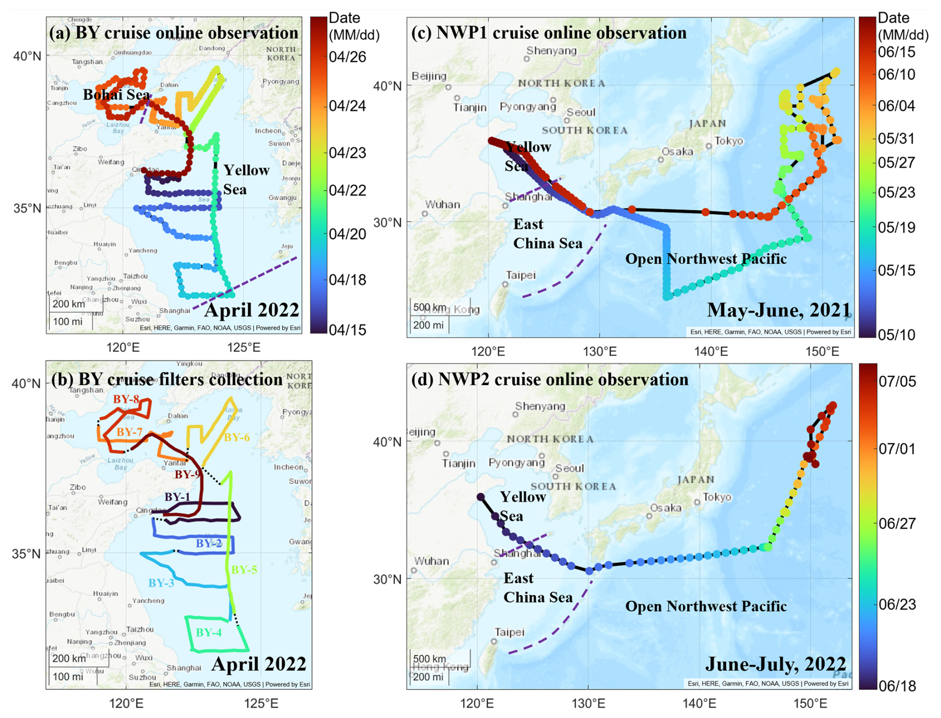
Figure 1 Cruise tracks in the Chinese marginal seas and the open Northwest Pacific during 2021–2022. (a) Shipborne online observations during the BY cruise, where each dot represents an online sample, and the colour indicates the sampling date; (b) Filter sample collection during the BY cruise, where each solid line represents an offline filter sample; (c) and (d) Shipborne online observations during the NWP1 and NWP2 cruises, respectively, analogous to panel (a). BY denotes the cruise conducted in 2022 over the Bohai Sea and Yellow Sea, while NWP1 and NWP2 denote cruises conducted in 2021 and 2022, respectively, in the Northwest Pacific. For the NWP2 cruise track, only periods when the instrument was functioning normally are shown.

2.2 Shipborne online observations

During the three cruises, an online multi-element analyzer (Xact 625) was used to continuously measure elemental concentrations in atmospheric aerosols. The Xact 625 (Cooper Environmental Services LLC) is designed to monitor aerosol elemental composition at high time resolution (Yanca et al., 2006) and has been certified by the U.S. Environmental Protection Agency (EPA) for ambient air monitoring (https://archive.epa.gov/nrmrl/archive-etv/web/pdf/p100fk6b.pdf, last access: 10 September 2025). The instrument operates at an air sampling flow rate of 16.7 L min⁻¹. Ambient aerosols pass through a size-selective inlet and then flow through the instrument tubing before being deposited onto a reel-to-reel polytetrafluoroethylene (PTFE) filter tape. The sampling duration (time resolution) of each sample is adjustable between 0.5 and 4 h. After each sampling cycle, the reel advances to move the filter tape segment with the sample spot to the analysis position. Elemental masses of various target elements at the sample spot are automatically determined using a built-in X-ray fluorescence (XRF) system. The instrument calculates ambient mass concentrations of each element based on the sampling duration and flow rate. The Xact 625 used in this study is capable of simultaneously analyzing 22 elements, including K, Fe, Ca, Zn, Mn, Ba, Cu, Pb, V, Ni, As, Se, Ag, Cd, Cr, Hg, Co, Sn, Sb, Ga, Au, and Tl.

During the NWP1 and NWP2 cruises, the Xact 625 instrument was installed inside a container on the foredeck, with the sampling inlet fixed to the container roof, approximately 12 m above sea level (m a.s.l.). As shown in Fig. S1, the inlets were positioned forward of the ship's funnel and at a lower height, minimizing the influence of the ship's exhaust plume, which typically dispersed aft and upward. During the BY cruise, the research vessel was not equipped with a foredeck container. Therefore, the Xact 625 had to be installed in a laboratory on the main deck, with the sampling inlet secured to the portside railing of the boat deck, approximately 10 m a.s.l. The relatively long sampling tubing connecting the inlet to the instrument may have caused particle losses due to impaction on the inner walls, likely leading to an underestimation of coarse-mode crustal elemental concentrations during periods of extremely high dust loadings. However, the impact of this underestimation on source apportionment results for this period is considered limited. Further discussion is provided in Sect. S1 in the Supplement.

For particle size selection, the Xact 625 was equipped with a PM_2.5 inlet during the NWP1 cruise, which selectively sampled fine particles with aerodynamic diameters less than or equal to 2.5 µm. In contrast, a PM₁₀ inlet was used during the BY and NWP2 cruises to extend the measurements to coarse particles with aerodynamic diameters less than or equal to 10 µm. This size range is also comparable to those covered in several aerosol models, such as CAM (0.1–10 µm), CMAQ (0.1–10 µm), GEOS-Chem (0.1–12 µm), and IMPACT (<1.26–20 µm) (Binkowski and Roselle, 2003; Myriokefalitakis et al., 2018).

The temporal resolution of the measurements was also adjusted according to ambient conditions. During the BY cruise, where elemental concentrations were relatively high and the cruise track was short, the resolution of Xact 625 was set to 1 h and further refined to 0.5 h in parts of the northern Yellow Sea to maximize data collection. In contrast, during the NWP1 cruise, the resolution was set to 2 h in marginal seas and 4 h over the open Northwest Pacific. In the summer NWP2 cruise, when elemental concentrations were lower, the resolution was set to 4 h, which ensured the lowest detection limits.

2.3 Filters collection and laboratory analysis

In addition to shipborne online observations, filter samples were collected during the BY cruise using a TH-16A sampler (Wuhan Tianhong Environmental Protection Industry Co., Ltd.). The TH-16A features four sampling channels, each operating at a constant flow rate of 16.7 L min⁻¹. In this cruise, each channel of the TH-16A was equipped with a PM₁₀ inlet, enabling the sampling of particulate matter with aerodynamic diameters ≤10 µm. PTFE filters (46.2 mm diameter, Whatman) were used to collect atmospheric particulate matter. As shown in Fig. S1, the sampler was installed on the compass deck, located away from the ship's funnel to reduce potential contamination. Sampling was carried out only during vessel navigation and was paused while the ship was anchored. Each filter sample represented a cumulative 24 h sampling period. In total, nine PM₁₀ filter samples were collected during the BY cruise (see BY1–BY9 in Fig. 1b).

Both total and soluble elements in the filters were analyzed. Detailed procedures are provided in the Supplementary Material (Sect. S2). Briefly, total elements were extracted by microwave-assisted acid digestion using a mixture of nitric acid (HNO₃), hydrogen peroxide (H₂O₂), and hydrofluoric acid (HF) (Zhang et al., 2022). After digestion, the solution was heated to near dryness and reconstituted with 20 mL of 1 % ($v/v$) HNO₃, followed by filtration through a 0.22 µm polyethersulfone (PES) syringe filter. Soluble elements were extracted by horizontally shaking the filter fragments for 2 h in an ammonium acetate–acetic acid buffer (pH 4.7) at room temperature. Compared to deionized water, this buffer better simulates Fe dissolution in ligand-added leaching conditions (Perron et al., 2020). The resulting solution was filtered through a 0.22 µm PES syringe filter and acidified to 1 % ($v/v$) HNO₃. Both total and soluble elemental extracts were analyzed using inductively coupled plasma mass spectrometry (ICP-MS; iCAP Q, Thermo Fisher Scientific) for the concentrations of Al, Fe, Ba, Mn, Cr, Cu, Zn, Pb, V, Ni, As, Se, Cd, and Sb.

2.4 Data quality control

2.4.1 Data quality control of Xact 625 online measurements

The data quality control procedures for the Xact 625 measurements are described in detail in our previous study (Zhang et al., 2024). In summary, the quality control process involved three key steps: (1) calibration of the Xact 625 instrument using elemental standards with certified concentrations, followed by verification of instrumental stability through manual review of automated quality control (QC) logs; (2) evaluation of the proportion of samples with elemental concentrations above the minimum detection limits (MDL) for 22 elements, alongside the identification and removal of outliers; and (3) exclusion of samples potentially influenced by ship exhaust, based on apparent wind direction and apparent wind speed criteria.

The quality control results from Step 1 indicated stable operation of the Xact 625 instrument during the BY and NWP1 cruises. However, a mid-cruise instrument malfunction occurred during the NWP2 cruise. As shown in Fig. S3, both the QA-Pd values (used to monitor XRF fluorescence intensity) and the stability of the built-in Cr, Pb, and Cd reference rods, which were automatically measured through daily QC protocols, deviated significantly after 6 July 2022. These deviations indicate that the instrument was no longer operating under normal conditions, resulting in unreliable measurements. Therefore, for the NWP2 cruise, only data collected between 18 June and 6 July were discussed in this study. In addition, blank tests were conducted on the PTFE filter rolls used in the Xact 625 during each cruise. The results showed abnormally high blank values for K in both the BY and NWP2 cruises. As a result, K data from these two cruises were excluded from further discussion in this study.

The quality control (QC) results from Step 2 showed that the concentrations of the target element (Fe) in all samples from the three cruises were above the MDL. In addition to Fe, other elements were mainly used as input variables in the Positive Matrix Factorization (PMF) receptor model to assist in source identification of Fe. According to Huang et al. (1999), chemical species used as input data for the PMF model should have more than 80 % of their values above the MDL. Therefore, twelve elements that met this criterion were initially selected. These included K (only for the NWP1 cruise), Ca, Mn, Fe, Ni, Cu, Zn, Se, Au, Cd, Ba, and Pb. Among these elements, Au was excluded due to the lack of understanding of its emission sources. Cd was further excluded due to low confidence in its concentration measurements, as its concentrations were significantly higher than those reported in previous studies (Table S3). Instead, the specific tracers of ship emission (V) (Zhao et al., 2013) and coal combustion (As) (Tian et al., 2015) were additionally selected, although they only have 75 % and 39 % values above detection limits. Based on the time series of these elemental concentrations, five outliers were identified. These included two for Ca, two for Ba, and one for Zn. The outliers were replaced with the average concentrations of the corresponding elements in the samples immediately before and after the outliers. Details on the definition and screening method of outliers are provided in Sect. S3 in the Supplement.

In Step 3, samples potentially contaminated by ship exhaust from the research vessel were identified through a two-step procedure. First, 8 samples with an average apparent wind speed (vector sum of real wind and ship wind) below 2 m s⁻¹ were excluded (Gao et al., 2013; Zhang et al., 2024). Second, 75 samples were selected only if, during the respective sampling cycle, the inlet was occasionally located downwind of the ship's funnel due to the apparent wind blowing from the stern toward the bow, and the apparent wind speed was maintained at a minimum of 2 m s⁻¹ for at least 5 min. Using V and Ni as tracers for ship smoke (Zhao et al., 2013), it was found that 14 of the 75 selected samples exhibited concentrations of V and Ni that exceeded the cruise-averaged values. These 14 samples were considered potentially contaminated by ship smoke and were excluded from further analysis. As a result, a total of 644 valid samples remained out of the original 666 samples.

2.4.2 Data quality control of filter chemical analysis

For elemental analysis of the filter samples in the laboratory, two certified standard reference materials of Luochuan loess from Shaanxi, China (GBW07454 (GSS-25), certified Fe content: 3.01 ± 0.05 %) were digested alongside the ambient aerosol samples. Based on the specific aliquots used, the certified total Fe contents of the two reference materials were 189.44–195.84 and 180.56–186.66 µg, respectively. The Fe concentrations measured by ICP-MS were 192.26 and 182.32 µg, respectively, both of which fell within the certified ranges, thereby confirming the accuracy of the analytical procedure. In addition, internal standard elements (Sc, Ge, Y, and In) were spiked into the test solutions during ICP-MS analysis. The recovery rates of these internal standards were consistently maintained within the range of 80 %–120 % across all samples, further validating the reliability of the analysis.

Four field blanks were analyzed, including two blanks for acid digestion and two for buffer extraction. Elemental concentrations in ambient samples were corrected by subtracting the corresponding blank values. For the elements discussed in this study (Al, Pb, V, Fe, and soluble Fe), concentrations in the blank samples contributed relatively little to those in ambient samples. Specifically, the average concentrations of Al, Pb, V, Fe, and soluble Fe in blank samples accounted for 1.7 %, 4.0 %, 7.2 %, 13.4 %, and 0.29 % of their respective concentrations in ambient samples.

2.5 Source apportionment receptor model

The Positive Matrix Factorization receptor model was applied using the U.S. EPA PMF version 5.0 software to apportion the sources of Fe in marine aerosols. As a multivariate factor analysis tool, the PMF model does not require the input of source profiles, but relies on chemical tracers to identify emission sources (Paatero and Tapper, 1994; Gary et al., 2014). The PMF model requires two key inputs: a measured species concentration matrix (X) and their associated uncertainty values, which are used to weight individual data points. The methodology for calculating uncertainties is provided in Sect. S4 in the Supplement. As shown in Eqs. (1) and (2), PMF decomposes the species concentration matrix (X) into a factor contribution matrix (G) and a factor profile matrix (F) by minimizing the objective function Q using a weighted least squares approach. Source identification is carried out by interpreting the chemical tracer signatures in the factor profiles (matrix F) and the factor contributions (matrix G) is used to quantitatively apportion contributions of each source.

$$\begin{array}{}\text{(1)}& {\displaystyle }\mathbf{X}=\mathbf{GF}+\mathbf{E}\text{(2)}& {\displaystyle }Q\left(\mathbf{E}\right)={\sum }_{i=\mathrm{1}}^n{\sum }_{j=\mathrm{1}}^m{\left[{\displaystyle \frac{e_{ij}}{u_{ij}}}\right]}^{\mathrm{2}}\end{array}$$

where matrix X (species concentrations) has dimensions n×m, where n is the number of samples and m is the number of chemical species; matrix G (factor contributions) has dimensions n×p, where p represents the number of factors (emission source types); matrix F (factor profiles) has dimensions p×m, describing the chemical composition of each factor; matrix E (residual matrix) also has dimensions n×m and represents the difference between the measured concentrations (X) and the model-reconstructed values (GF); e_ij and u_ij in Eq. (2) are the residuals and uncertainties of the species j in sample i, respectively.

The PMF has been successfully applied to investigate Fe sources in urban aerosols (Zhu et al., 2022; Meng et al., 2023; Zhang et al., 2025). However, PMF requires a relatively large sample size, typically at least five times the number of input chemical species, therefore generally requiring 50 samples or more (Cao, 2014). This requirement has consequently constrained its application in ship-based studies, where the number of offline filter samples is often insufficient. Therefore, the application of PMF in marine aerosols studies has primarily relied on the integration of multi-cruise offline datasets (Wang et al., 2013), long-term observations at fixed island stations (Li et al., 2023b), or shipborne online measurements (Zhang et al., 2024).

3 Results and discussions

3.1 Sources of total Fe in marine aerosols

3.1.1 Source apportionment of total Fe by PMF

As described in the Methodology section, quality-controlled datasets were incorporated into the PMF analysis. Specifically, 229 online PM_2.5 samples containing 12 elements from the NWP1 cruise, 97 online PM₁₀ samples containing 11 elements from the NWP2 cruise, and 318 online PM₁₀ samples containing 11 elements from the BY cruise were used. The NWP1 cruise uniquely included K in its elemental dataset, which was absent in the other two campaigns. In addition, NWP1 targeted PM_2.5 fraction measurements, whose source profiles may differ from those of PM₁₀ particles (Zhang et al., 2014b). For these reasons, the NWP2 and BY cruise datasets were processed together in the PMF model, whereas the NWP1 cruise data were processed separately. The optimal number of PMF factors was determined based on mathematical diagnostic indicators from the PMF Guide and on the variations of chemical tracers in each factor. Further details are provided in Sect. S5 in the Supplement. In brief, the results indicated that three factors provided the best fit. The corresponding factor profiles are presented in Fig. 2.

As depicted in Fig. 2a, the three-factor profiles derived from marine atmospheric PM₁₀ samples in this study exhibited three clearly distinct emission sources. Factor 1 showed a significant contribution (>50 %) to elements Ca, Fe, and Ba, indicating a clear dust source signature (Zhang et al., 2014b; Bi et al., 2019; Zhang et al., 2023b). Factor 2 demonstrated substantial contributions to multiple elements, including Mn, Cu, Zn, Pb, As, and Se, representing emissions from land anthropogenic activities, such as industrial processes and coal combustion (Tian et al., 2015; Liu et al., 2018). Factor 3 was characterized by high contributions to V and Ni, established tracers of heavy oil combustion, indicating its origin from ship emission (Zhao et al., 2013; Yu et al., 2021). The three-factor profiles for PM_2.5 samples, presented in Fig. 2b, were similar to those of PM₁₀, with only minor differences in the concentrations and contribution percentages of certain elements within the factors. These PM_2.5 factor profiles also represented the same three source categories, namely dust, land anthropogenic, and shipping sources.

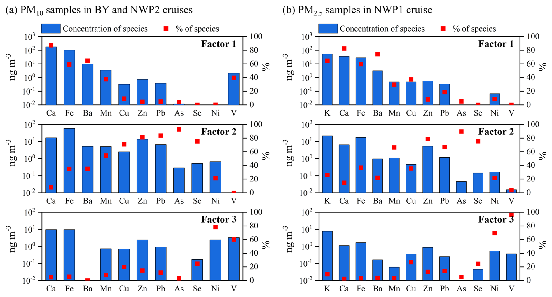
Figure 2 Factor profiles (blue bars) and average factor contributions (red squares) output by the PMF model. (a) PM₁₀ samples from the BY and NWP2 cruises. (b) PM_2.5 samples from the NWP1 cruise.

3.1.2 Comparison of filter-based chemical tracers with PMF results derived from online measurements

Previous traditional filter-based studies often had small sample sizes, which limited the use of receptor models in earlier work. Researchers therefore relied on chemical tracers for qualitative source identification of marine aerosols. Common choices included Al as a dust tracer, Pb as an indicator of land-based anthropogenic pollution, and V as an indicator of ship emission from heavy oil combustion (Hsu et al., 2010; Guo et al., 2014; Lee et al., 2017). In this study, we compared PMF-resolved Fe from the Xact 625 online measurements with these filter-based tracers during the BY cruise to evaluate how well these tracers captured source-specific Fe concentrations. The filter samples were aligned in sampling time with the online observations, and the PMF-resolved Fe concentrations were plotted against the concentrations of Al, Pb, and V measured on the filters (Fig. 3).

As shown in Fig. 3a and b, Al and Pb demonstrated strong capability as tracers for dust-derived Fe and land anthropogenic Fe, respectively. The corresponding linear regression analyses yielded R² of 0.99 and 0.83, respectively. In contrast, the R² for the linear regression between V and ship-derived Fe concentration was lower, at 0.68 (Fig. 3c). Inspection of the scatter plot for ship-derived Fe versus V identified an outlier (circled with a dashed line) positioned below the regression line, indicating a higher V concentration relative to its ship-derived Fe level. This suggests that an additional source contributed V to this sample. This sample (BY9, Fig. 1b) was collected during an intense dust event transported from East Asia (see Sect. 3.1.3). Filter analysis showed an Al concentration of 3011 ng m⁻³, indicating substantial dust influence. The $\mathrm{Al}/\mathrm{V}$ ratio for this sample was 420, close to the crustal ratio of 691 (Li and Yuan, 2011) and much higher than the average ratio in other samples (31.9 ± 31.9). These results suggest that intense dust events elevated V concentrations in this sample.

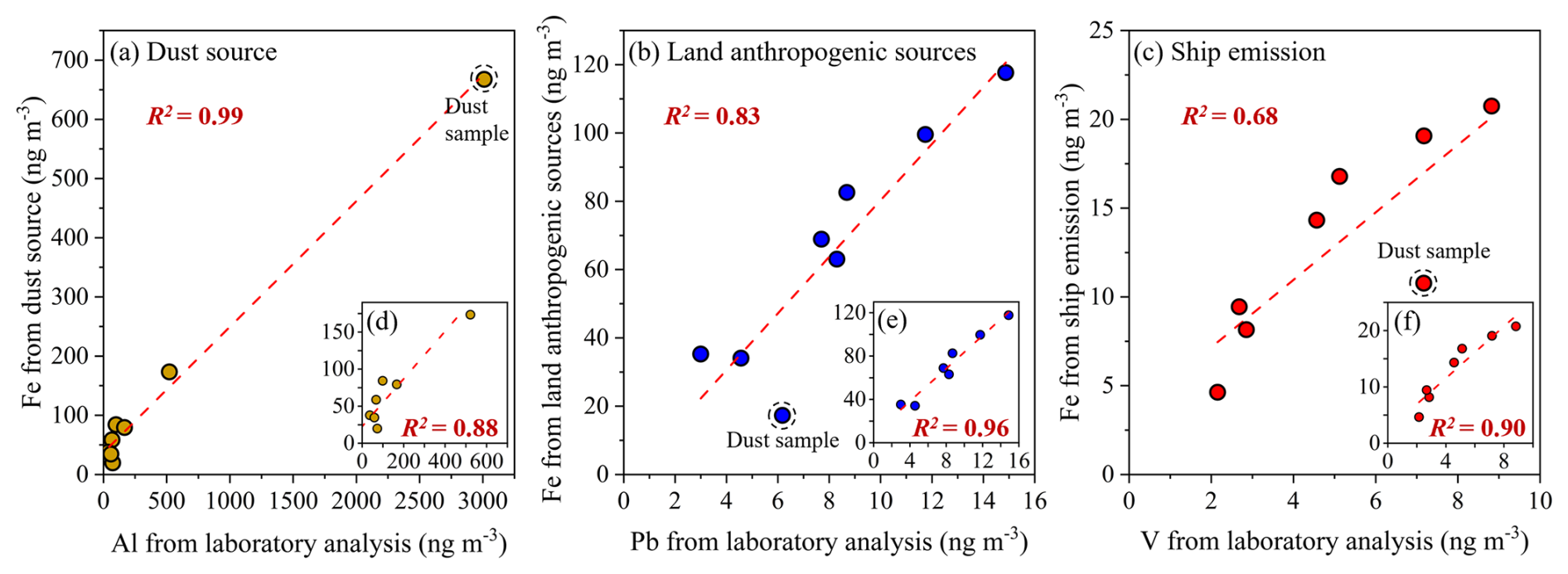
Figure 3 Comparing PMF results from Xact 625 online measurements with chemical tracers from offline filter analyses. (a) Fe concentration from dust source versus Al concentration. (b) Fe concentration from land anthropogenic sources versus Pb concentration. (c) Fe concentration from ship emission versus V concentration. (d)–(f) same as (a)–(c), but excluding the dust sample data point. The dashed circle represents the dust sample, and the red dashed lines represent the linear regression lines for these scatter plots.

When the dust-affected sample was excluded, the R² for ship-derived Fe versus V increased markedly from 0.68 to 0.90 (Fig. 3c and f), while the R² for land anthropogenic Fe versus Pb improved from 0.83 to 0.96 (Fig. 3b and e). Conversely, the R² for dust-derived Fe versus Al decreased slightly from 0.99 to 0.88 (Fig. 3a and d). This pattern reinforces that dust events strengthen the applicability of Al as a dust tracer but reduce the reliability of non-dust tracers, particularly V for ship emission. Using V to directly trace ship-derived particles during periods or in regions with high dust influence may therefore lead to overestimation. We further examined the relationship between ship-derived Fe and another commonly used tracer for ship emission, Ni. Excluding the dust-affected sample changed the R² of their linear regression from 0.55 to 0.60 (Fig. S5), indicating a limited dust influence on Ni. Nevertheless, the overall correlation between Ni and ship-derived Fe remained weaker than that between V and ship-derived Fe, which supports the higher relative contribution of ship emission to V than to Ni in the Northwest Pacific, as revealed by modelling (Jiang et al., 2024).

These findings illustrate the limitations of directly using filter-based chemical tracers to identify source-specific Fe (or other species). Receptor models such as PMF are preferable, as they provide quantitative source apportionment that accounts for tracer overlap among sources. While PMF still uses tracers to identify source categories, its results typically indicate that the traced source is the primary, but not the sole, contributor to the tracer. For example, in Fig. 2a, V had the highest loading in the ship emission factor (factor 3) but also appeared in the dust factor (factor 1) due to dust event interference. Such source apportionment better captures the complexity of the real-world atmospheric environment. Moreover, because PMF is driven by observational data, it generally yields more reliable results than purely numerical models.

3.1.3 Sources of atmospheric total Fe in Chinese marginal seas

The Bohai Sea and Yellow Sea lie adjacent to mainland China, roughly between 30 and 40° N. Under the prevailing westerlies, dust emissions from northern China and Mongolia can be transported to these regions (Zhang et al., 2023b; Ji et al., 2024). Owing to their proximity to the North China Plain, the Bohai Sea and Yellow Sea are also strongly influenced by anthropogenic pollutants (Liu et al., 2022a; Xu et al., 2023), resulting in complex aerosol sources.

Ship-based online measurements of atmospheric Fe conducted in April 2022 (Fig. 4a) showed Fe concentrations in PM₁₀ samples ranging from 25.34 to 2874 ng m⁻³, with a median value of 133.2 ng m⁻³. Along the cruise track, the mean Fe concentration was 130.9 ± 74.64 ng m⁻³ in the Bohai Sea and 247.6 ± 302.5 ng m⁻³ in the Yellow Sea. Overall, these values were comparable to recent shipborne observations in nearby sea areas. For example, Yang et al. (2020) reported an Fe concentration of 543.1 ng m⁻³ in atmospheric TSP (total suspended particulates) over the Yellow Sea–East China Sea region in spring 2017, and Ge et al. (2024) reported a value of 258 ng m⁻³ of Fe in atmospheric TSP over the East China Sea in autumn 2021.

However, compared with much earlier measurements, the Fe concentrations observed during this cruise were lower. For instance, Zhang et al. (2014a) reported a mean Fe concentration of 728.2 ng m⁻³ in PM_2.5 over Tuoji Island in the Bohai Sea in spring 2012, and Wang et al. (2013) reported a mean Fe concentration of 2102 ± 608.9 ng m⁻³ in atmospheric TSP over the northern Yellow Sea based on shipborne sampling in spring 2007. Such differences might reflect interannual variability in atmospheric Fe concentrations over the Chinese marginal seas. This inference was supported by the model-simulated decline in dust-derived Fe transport from East Asia to the oceans during 2001–2017 (Zhu et al., 2025) and with the reported decrease in anthropogenic metals deposition in Chinese marginal Seas from 2012 to 2019 (Zhang et al., 2023a).

During the BY cruise, three high-Fe-concentration episodes (EP1, EP2, and EP3) were identified. These episodes were defined as periods during which Fe concentrations exceeded the 75th percentile of all samples collected during the cruise (218.2 ng m⁻³) and persisted for more than 12 h. The spatial distribution and timing of these episodes are shown in Fig. 4a and b, respectively. EP1, EP2, and EP3 lasted 26.5, 16.5, and 23 h, respectively (EP3 observations were truncated due to cruise termination), with corresponding mean Fe concentrations of 482.4 ± 537.8, 416.2 ± 90.54, and 906.2 ± 286.2 ng m⁻³. As shown in Fig. S6, the crustal element Ca exhibited trends similar to Fe during these episodes, with elevated Ca levels indicating dust influence. However, in EP1, the increase in Ca was markedly smaller than that of Fe, implying substantial contributions from non-dust sources. In contrast, pollution-related elements (Zn, Pb, and As) were abundant during EP1 and EP2 but occurred at very low levels during EP3, suggesting that EP3 represented a pure dust event.

Satellite remote sensing and backward trajectory analyses confirmed that air masses during all three episodes originated from inland East Asia (Figs. S7 and S8), indicating that continental air masses transport can trigger rapid and substantial increases in marine atmospheric Fe concentrations. In particular, high-time-resolution measurements during EP3 recorded an approximately 13-fold increase in Fe concentration within just 9 h, rising from 80.50 to 1111 ng m⁻³. This sharp rise coincided with a large-scale dust outbreak over northern China. According to the China Meteorological Administration (2022), this dust event affected Inner Mongolia, Ningxia, Gansu, Beijing, and Liaoning from 25 to 27 April 2022. The subsequent transport of this dust-laden continental air mass to the Bohai Sea and Yellow Sea (Fig. S7e and f) played a dominant role in driving EP3.

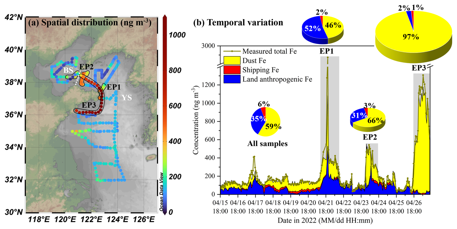
Figure 4 Spatiotemporal distribution of Fe concentrations in atmospheric PM₁₀ over the Bohai Sea and Yellow Sea in April 2022. (a) Spatial distribution of Fe concentrations. (b) Time series of measured total Fe and PMF-resolved Fe concentrations from different sources. EP1, EP2, and EP3 refer to three high-Fe-concentration episodes encountered during the observation period, whose spatial coverage and temporal ranges are indicated by black circles in (a) and shaded areas in (b), respectively. The four pie charts in (b) represent the proportion of Fe from different sources for the entire cruise and three episodes, respectively (figure generated using Ocean Data View; Schlitzer, 2025).

The PMF source apportionment results indicated that atmospheric Fe along the cruise tracks in Bohai-Yellow Sea primarily originated from dust source (mean contribution was 59 %), followed by land anthropogenic sources (35 %), with minimal input from ship emission (6 %). Figure 4b shows temporal variations in Fe concentrations from different sources. Non-dust sources contributions were significant in most samples except during EP3. During the three episodes of elevated Fe concentrations, distinct source characteristics were identified. EP1 exhibited a mixed dust–anthropogenic signature, with the highest non-dust contributions to individual sample reaching 85 % (mean was 54 %). EP2 initially showed dust dominance, later shifting toward non-dust sources (mean of non-dust contributions was 34 %). Conversely, EP3 was characterized by near-exclusive dust contributions (97 %). Because these episodes were associated with continental air mass transport, the proportion of ship-derived Fe during the events decreased to 1 %–3 %, below the cruise average (6 %).

Figure 5 shows the spatial distribution of Fe concentrations from different sources as determined by PMF analysis. Dust-derived Fe concentrations exhibited pronounced peaks during EP2 and EP3, reaching 283.5 ± 110.2 and 801.5 ± 283.6 ng m⁻³, respectively, while remaining much lower during other periods (55.71 ± 55.49 ng m⁻³). Although global model simulations have indicated that the meridional peak of East Asian dust transport to the ocean occurs near 40° N (Ito et al., 2019; Zhu et al., 2025), observations in this study showed higher dust-derived Fe contributions over the lower-latitude Yellow Sea (62 %) than over the Bohai Sea (34 %) (Fig. 5a). This largely resulted from two episodic high-dust events (EP2 and EP3), which substantially increased the average dust contribution in the Yellow Sea. However, even after excluding these two episodes, the average dust contribution in the Yellow Sea remained 40 %, slightly above that of the Bohai Sea, highlighting the relatively greater importance of non-dust sources in the Bohai Sea.

Figure 5 Spatial distributions of atmospheric Fe from different sources over the Bohai and Yellow Seas during the BY cruise. (a) Dust source Fe, (b) land anthropogenic source Fe, and (c) shipping source Fe. Pie charts in (a) show the mean percentage contributions of each source in the Bohai Sea (BS) and Yellow Sea (YS) (figures generated using Ocean Data View; Schlitzer, 2025).

The contrasting spatial distributions of Fe concentrations from different sources resulted in spatial variations of atmospheric source structures, with the non-dust contribution in the Bohai Sea (66 %) higher than that in the Yellow Sea (38 %) (Fig. 5a). The spatial patterns of land anthropogenic Fe and ship-derived Fe also differed. High ship-derived Fe concentrations were observed mainly in the Bohai Sea and the southern Yellow Sea. The Bohai Rim and the Yangtze River Delta hosted major port clusters, and the rapid growth of maritime trade caused substantial ship emission (Chen et al., 2017). As shown in Fig. S8, air mass back trajectories above the sampling area in southern Yellow Sea passed through the Yangtze River Delta, which explained the higher ship-derived Fe concentrations there.

In the central Yellow Sea, a south to north shipping route was associated with high ship-derived Fe concentrations during 19–20 April. During this period, numerous vessels, predominantly small fishing boats, were observed within visual range of the research vessel (Fig. S9). Although previous source tests indicated that small fishing boats had lower V emission factors than ocean-going vessels (Zhang et al., 2018), such a dense cluster of emission sources around the research vessel was likely one reason for the elevated concentrations of V (14.27 ± 8.75 ng m⁻³) and ship-derived Fe (22.34 ± 4.82 ng m⁻³) recorded along this transect. Similar observational results regarding the contribution of ship-derived Fe were reported by Qi et al. (2025), with ship emission contributing 10 % of atmospheric Fe in PM_2.5 over the Bohai and Yellow Seas in spring 2018, which is comparable to the 6 % contribution derived from PM₁₀ samples in this study.

3.1.4 Sources of atmospheric total Fe in Northwest Pacific Ocean

Located downwind of East Asia, the Northwest Pacific is strongly influenced by continental aerosols outflow (Yu et al., 2020). To characterize atmospheric Fe in the region, we conducted two shipboard campaigns with online measurements (Fig. 1c and d). The first campaign (NWP1) was carried out in May–June 2021 and measured PM_2.5 samples, and the second (NWP2) was conducted in June–July 2022 and measured PM₁₀ samples.

During the NWP1 cruise, Fe concentrations ranged from 2.60 to 401.7 ng m⁻³, with a median of 36.70 ng m⁻³ and a mean of 54.90 ± 52.48 ng m⁻³. Most high-Fe-concentration samples were clustered along the Yellow Sea and East China Sea (YES) leg (Fig. 6a). A few elevated values also appeared over the open Northwest Pacific, particularly in the mid-latitude oceanic area east of Japan between 37 and 39° N. A pronounced high-Fe-concentration episode occurred in this area from 26 to 28 May, with a peak of 401.7 ng m⁻³ (Fig. 6b). Similar to this phenomenon, our previous work reported two high-Fe-concentration events east of Japan during a spring 2015 cruise (Zhang et al., 2024), suggesting that this region served as an important receptor of continental aerosols outflow.

Source apportionment indicated that dust was the dominant contributor during NWP1, accounting for an average of 60 % of total Fe, followed by land anthropogenic sources (37 %) and ship emission (3 %). The non-dust contribution was higher in the YES region near the East Asian continent. During YES1 leg in May 2021, land anthropogenic sources and ship emission contributed 48 % and 4 % on average, respectively, and during YES2 leg in June 2021, they contributed 52 % and 16 %, respectively. Overall, non-dust sources contributed 40 % on average in NWP1 cruise, which was higher than our spring 2015 cruise result based on PM_2.5 online measurements and PMF analysis (31 %) (Zhang et al., 2024), but lower than the modeled contribution of 59 % simulated by CMAQ for the open Northwest Pacific in April 2017 (Jiang et al., 2024).

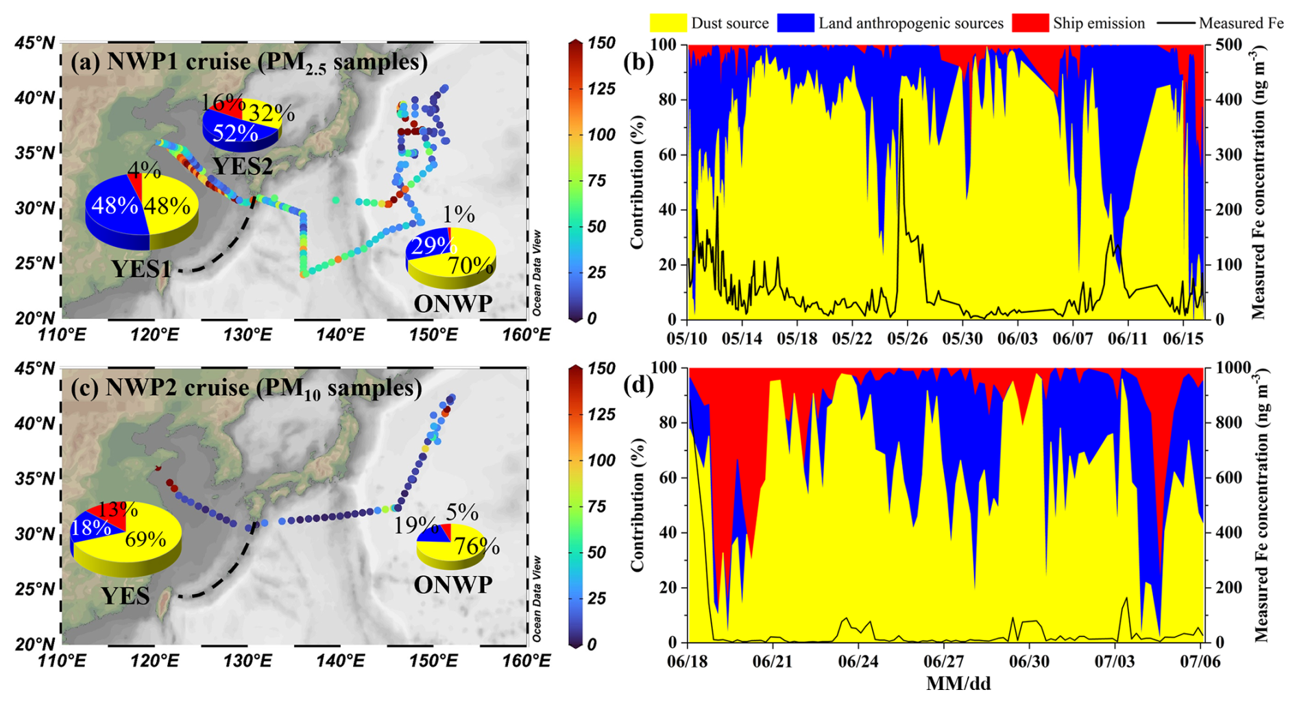
Figure 6 Concentration and sources of atmospheric total Fe over the Northwest Pacific. (a) Fe concentrations (ng m⁻³) in atmospheric PM_2.5 during the NWP1 cruise in 2021. (b) Time series of Fe concentration and source composition during NWP1 cruise. (c) and (d) correspond to (a) and (b), respectively, but represent Fe in atmospheric PM₁₀ during the NWP2 cruise in 2022. The pie charts in (a) and (c) show the average source proportions of Fe for different sea areas. YES denotes the Yellow Sea and East China Sea, and ONWP denotes the open Northwest Pacific east of the black dashed line in (a) and (c) (figures generated using Ocean Data View; Schlitzer, 2025).

During the NWP2 cruise, Fe concentrations ranged from 2.00 to 883.2 ng m⁻³, with a median of 10.58 ng m⁻³ and a mean of 35.56 ± 99.94 ng m⁻³. Although NWP2 collected PM₁₀ samples, both the mean and the median Fe concentrations were lower than those in PM_2.5 samples in NWP1. High concentrations of 145.9–883.2 ng m⁻³ were recorded on the departure day, 18 June, whereas subsequent samples along the Yellow Sea and East China Sea legs averaged only 7.97 ± 3.08 ng m⁻³, far below the values in YES region during NWP1 (76.35 ± 52.40 ng m⁻³). Meteorological observations on board indicated peak hourly rainfall intensities of 11.85, 8.30, and 30.9 mm h⁻¹ on 18, 19, and 20 June, respectively. Under the influence of precipitation, Fe concentrations dropped sharply to below 10 ng m⁻³. At the same time, PMF results showed a rapid decrease in the fractional contribution from dust and a relative increase in the contribution from ship emission (Fig. 6d). These patterns indicated that wet deposition effectively scavenged atmospheric Fe, reducing the relative contribution of continentally transported material while enhancing the relative influence of local emissions such as ship exhaust. Consequently, rainfall-induced wet deposition was the primary reason for the lower Fe concentrations observed along the subsequent YES leg during NWP2. Regarding sources, non-dust contributions in NWP2 were lower than in NWP1, averaging 27 % over the entire cruise. Similarly, within NWP2, the coastal leg also showed a higher non-dust contribution (31 %) than the open-ocean leg (24 %) (Fig. 6c).

This study presents a further analysis of the causes of a high-Fe-concentration episode (EP) observed in the open Northwest Pacific Ocean during the NWP1 cruise. The episode, defined by Fe concentrations exceeding the 75th percentile (65.63 ng m⁻³) of the entire cruise dataset, persisted for approximately 48 h. During this period, Fe concentrations rose sharply, increasing from 52.36 ng m⁻³ at 02:00 GMT+8 on 26 May (prior to the EP) to 401.7 ng m⁻³ at 10:00 GMT+8 on the same day (Fig. 7c), representing nearly a 7-fold increase within just eight hours.

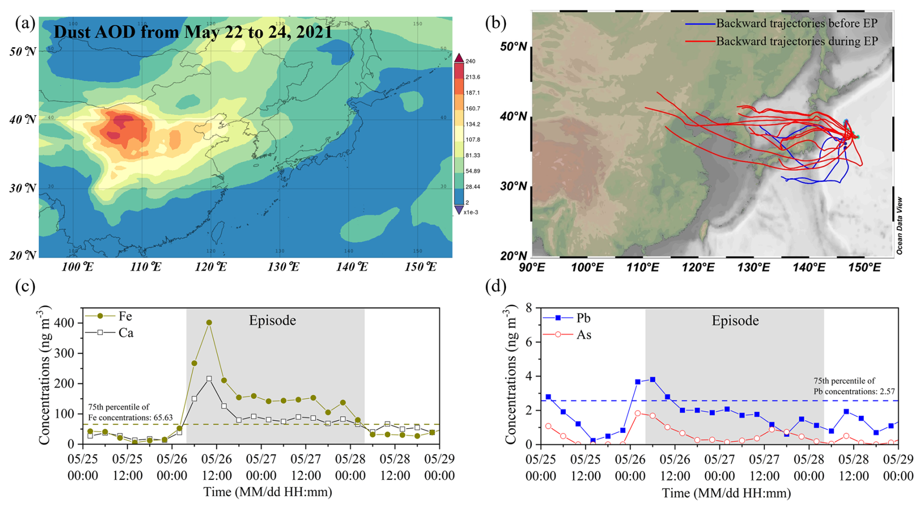
Figure 7 Chemical components and air mass origins of high-Fe-concentration episode in open Northwest Pacific. (a) Dust aerosols optical depth in East Asia during 22–24 May 2021, generated using the Giovanni online tool with MERRA-2 reanalysis data. (b) Seventy-two-hour backward air mass trajectories at 500 m altitude, with red lines representing trajectories during the high-concentration episode and blue lines representing those prior to the episode. (c) and (d) Variations in the concentrations of crustal elements (Fe, Ca) and pollution-derived elements (Pb, As) during and outside high-concentration episode, respectively (figure generated using Ocean Data View; Schlitzer, 2025).

The episode was likely associated with a dust event in northern China. According to the Chinese Meteorological Bulletin of Atmospheric Environment, a dust event affected central-western Inner Mongolia, Ningxia, northern Shanxi, Hebei, Beijing, and Tianjin from 22 to 24 May in 2021 (China Meteorological Administration, 2021). Dust aerosol optical depth (AOD) data from the Modern-Era Retrospective analysis for Research and Applications, Version 2 (MERRA-2) for the same period revealed the spatial extent of dust aerosols during the event (Fig. 7a). Backward trajectory analysis showed that, before the episode, air masses over the sampling region originated mainly from oceanic areas south of Japan and the Sea of Japan, whereas during the episode they were predominantly from the East Asian continent (Fig. 7b). This suggested that the long-range transport of dust-laden air masses from the continent was a significant contributor to the elevated Fe levels measured during the episode.

Compositional analysis of aerosols during the episode (Fig. 7c–d) further supported this conclusion. Fe showed a similar variation pattern to Ca, a crustal element, indicating a substantial contribution from dust to the elevated Fe. During the episode, average Fe and Ca concentrations were 3.2 and 2.2 times their respective mean values in the entire cruise. In contrast, pollution-related elements such as Pb and As exhibited smaller fluctuations, with average concentrations of 1.87 ± 0.83 and 0.58 ± 0.45 ng m⁻³, corresponding to only 1.0 and 1.5 times their respective cruise means. PMF results further indicated that the dust source accounted for 79 %–92 % of Fe in samples collected during the episode (Fig. 6b). Collectively, these results demonstrate that the high Fe concentrations observed in the open Northwest Pacific during this episode were predominantly driven by dust particles, with non-dust sources playing a comparatively minor role.

3.2 Sources of soluble Fe in marine aerosols

3.2.1 Apportioning soluble Fe sources by integrating total Fe sources and Fe solubility

Drawing on previous experimental (Fu et al., 2012; Tang et al., 2023), observational (Sholkovitz et al., 2012; Shi et al., 2020), and modelling studies (Ito, 2015; Ito and Miyakawa, 2023), which collectively demonstrate that both source and atmospheric aging processes are pivotal in regulating Fe solubility in aerosols, this study posited that Fe solubility in ambient aerosols is principally determined by initial source characteristics and atmospheric processing. This dependence can be quantitatively described by Eq. (3):

$$\begin{array}{}\text{(3)}& \mathrm{SFe}{\mathit{\%}}_i=\sum _{j=\mathrm{1}}^n\left(f_{i,j}\times \mathrm{SFe}{\mathit{\%}}_{j,\mathrm{e}}\right)+R\end{array}$$

where SFe %_i represents the Fe solubility in ambient aerosol sample i; f_i,j denotes the relative contribution of emission source j to total Fe content in sample i; SFe %_j,eindicates the initial Fe solubility from source j at emission; n is the number of source categories; R accounts for atmospheric aging processes, including acid dissolution, photo-induced redox reactions, and organic ligand-mediated solubility changes (Ito et al., 2021), which are difficult to quantify directly in current observational research.

To resolve source-specific effects of atmospheric aging on Fe solubility, we decomposed the aging parameter R, as formalized in Eq. (4). During transport from source regions to receptor sites, Fe from each emission source underwent atmospheric processing that increased its solubility. Equation (5) quantifies this enhancement of each source, where SFe %_j,e represents the initial Fe solubility from source j at emission, while SFe %_j,r denotes the Fe solubility at the receptor after atmospheric processing. After obtaining SFe %_j,r from Eq. (5), the calculation formula for Fe solubility in ambient aerosol samples is updated from Eqs. (3) to (6).

$$\begin{array}{}\text{(4)}& {\displaystyle }R=\sum _{j=\mathrm{1}}^n{R}_j\text{(5)}& {\displaystyle }\mathrm{SFe}{\mathit{\%}}_{j,\mathrm{r}}=\mathrm{SFe}{\mathit{\%}}_{j,\mathrm{e}}+R_j\text{(6)}& {\displaystyle }\mathrm{SFe}{\mathit{\%}}_i=\sum _{j=\mathrm{1}}^n\left(f_{i,j}\times \mathrm{SFe}{\mathit{\%}}_{j,\mathrm{r}}\right)\end{array}$$

Meanwhile, the relative contribution of source j to soluble Fe can be determined by combining total Fe sources and SFe %_j,r, as expressed in Eq. (7):

$$\begin{array}{}\text{(7)}& {\mathrm{Sf}}_{i,j}={\displaystyle \frac{f_{i,j}\times \mathrm{SFe}{\mathit{\%}}_{j,\mathrm{r}}}{\sum _{j=\mathrm{1}}^n(f_{i,j}\times \mathrm{SFe}{\mathit{\%}}_{j,\mathrm{r}})}}\end{array}$$

where Sf_i,j denotes the contribution of source j to soluble Fe in sample i; f_i,j represents the contribution of source j to total Fe in sample i; SFe %_j,r indicates the Fe solubility from source j at receptor following atmospheric aging.

In summary, two key inputs are required to determine the sources of soluble Fe using Eq. (7). The first is the fractional contribution of each emission source to total Fe in the ambient sample (f_i,j), and the second is the source-specific Fe solubility at the receptor (SFe %_j,r). In this study, f_i,j was obtained from the output of the PMF receptor model, and the determination and validation of SFe %_j,r are described in the next section.

3.2.2 Fe solubility parameterization and validation

Dust-source Fe solubility at receptor sites over oceanic regions was assessed by integrating observations from this study with those reported in previous literature. As described in Sect. 3.1.3, a severe dust event (EP3) occurred during the BY cruise, and the Fe solubility in the collected aerosol filter sample was 0.42 %. Using Fe isotope source apportionment method, Kurisu et al. (2021) quantified total and soluble dust-derived Fe over the open Northwest Pacific and reported a dust-derived Fe solubility of 0.9 %–1.3 % in the marine atmosphere, higher than our measurements in the Chinese marginal seas. Similarly, Takahashi et al. (2011) observed that, during transport of an East Asian dust plume from northwestern China to Japan, Fe solubility increased from 0.28 % to 1.1 %. Integrating these findings, the solubility of dust-derived Fe in aerosols over Chinese marginal seas was set at 0.5 % and that in the open Northwest Pacific was 1.0 %.

Observational data on the solubility of anthropogenic Fe in marine aerosols remain limited. This study referenced the solubility of combustion-derived Fe (11 %) over the open Northwest Pacific reported by Kurisu et al. (2021), setting the solubility of land anthropogenic Fe at 11 %. To be noted that, land anthropogenic Fe may originate from multiple sources, such as coal combustion, industrial emissions, and biomass burning (Chen et al., 2021; Zhang et al., 2025), with varied solubility of Fe. For example, PMF-based source apportionment of total and soluble Fe in PM_2.5 collected in Qingdao, China showed fly ash with 1 % solubility, while aged industrial emissions reached 12.5 % (Li et al., 2023a). Treating these diverse sources as a single category with one assigned solubility inevitably introduces uncertainty, representing a limitation of this approach. Future ship-based studies integrating online metal measurements with additional chemical tracers, such as water-soluble ions and organic species, are needed to resolve more detailed source categories.

For ship emission, which primarily originates from heavy oil combustion, the relatively short-range transport from ship emission sources to the receptors in marine atmosphere likely resulted in limited atmospheric aging. Therefore, we referred to source test results for heavy oil combustion, including 38 % (Desboeufs et al., 2001), 74.1 % and 85.9 % (Fu et al., 2012), and 77 % and 81 % (Schroth et al., 2009). In addition, Li et al. (2025a) reported a PMF-derived Fe solubility of 93.1 % for ship emission based on field observations in Qingdao, China. Based on these evidences, a ship-derived Fe solubility of 70 % was assumed as a conservative value in this study. For subsequent calculations, we assumed spatially uniform solubilities for land anthropogenic Fe and ship-derived Fe across the study domain and applied the same values to both the Chinese marginal seas and the open Northwest Pacific.

Using the SFe %_j,r parameters defined above, Fe solubility of ambient samples from the three cruises was calculated using Eq. (6). The calculated results were then compared with direct laboratory analysis of filters to validate the parameter settings. For the BY cruise, filter-based Fe solubility was compared with values calculated from online data. As shown in Fig. 8a, the two methods exhibited a strong linear correlation (R²=0.84). Their ranges and mean values were also closely matched, with 0.42 %–18.4 % (mean 10.9 % ± 5.4 %) for the laboratory analysis and 1.8 %–14.0 % (mean 10.7 % ± 4.2 %) for the calculations. The overall mean difference was only 0.2 percentage points.

Nevertheless, the measured Fe solubility during the BY cruise showed greater variability than the calculated values. For example, for samples BY3–BY6, the measured Fe solubility ranged from 11.5 % to 18.4 %, whereas the calculated values were in a narrower range (13.2 %–14.0 %). These four samples were collected from the southern, central, and northern Yellow Sea (Fig. 1b), and the greater variability in measured solubility likely reflects slight variations in atmospheric processing influence (R_j) and source-specific Fe solubility (SFe %_j,r) across the Yellow Sea. Such variations were relatively limited at this spatial scale. Therefore, using fixed SFe %_j,r still yield Fe solubility comparable to observations. At larger spatial scales (especially for global scale), however, such variations should be considered. As previously mentioned, to account for this, dust-derived Fe was assigned SFe %_j,r values of 0.5 % over the Chinese marginal seas and 1.0 % over the open Northwest Pacific, while land anthropogenic and ship-derived Fe were assigned to be constants due to insufficient observational constraints.

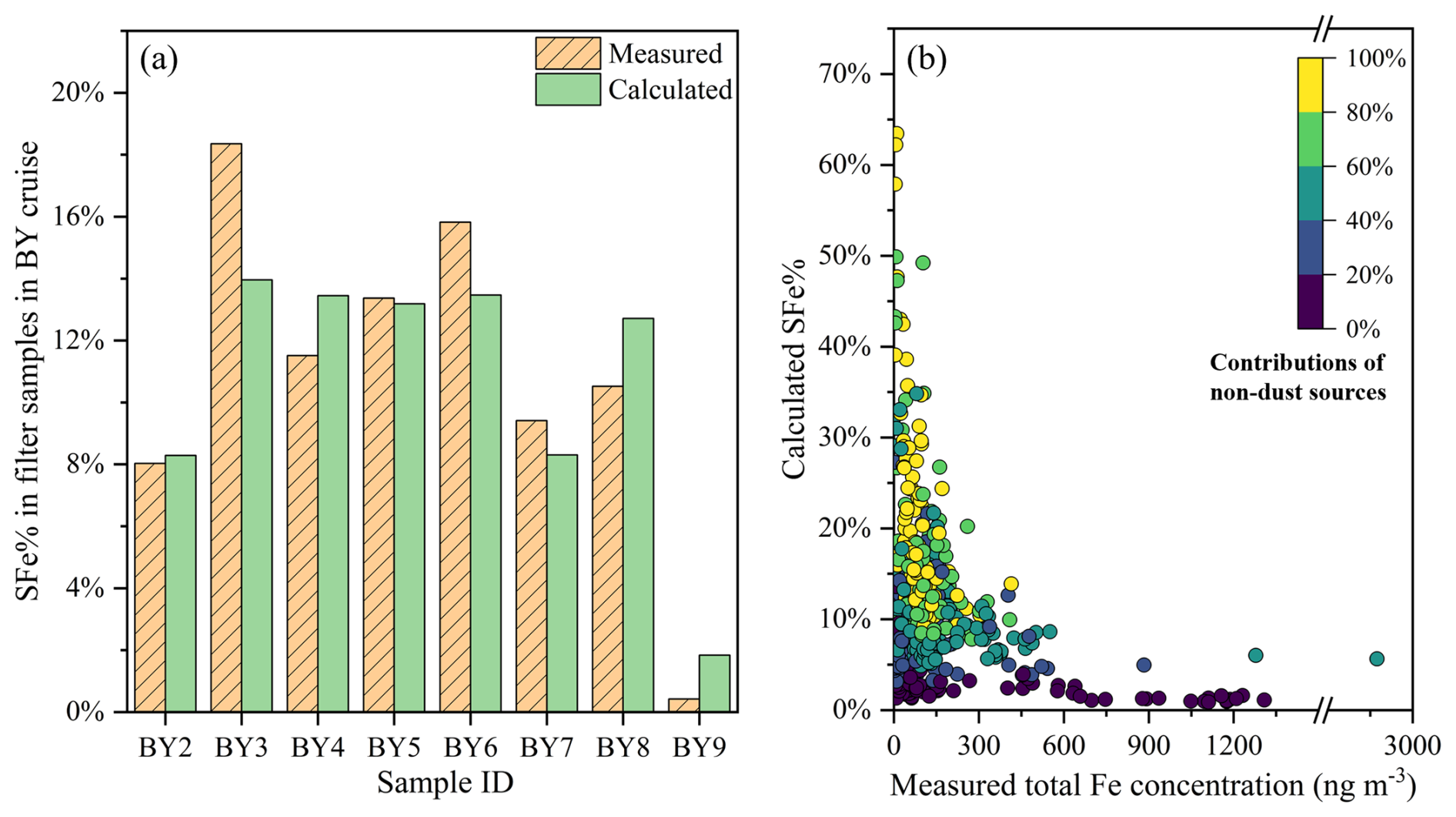
Figure 8 Validation of Fe solubility calculations. (a) Bar chart comparing measured and calculated Fe solubility for samples collected during the BY cruise; the BY1 filter sample was excluded because the online instrument data were incomplete during its sampling period. (b) Scatter plot of calculated Fe solubility versus measured total Fe for all three cruises; point colour indicates the fraction of non-dust Fe (sum of land anthropogenic and ship-derived sources) in total Fe.

Across 644 online samples collected during the three cruises, the calculated Fe solubility ranged from 0.89 % to 63.5 %. This range was comparable to our previous estimate of 1.1 % to 56.1 % in the Northwest Pacific during spring 2015 (Zhang et al., 2024), and it was consistent with Sholkovitz et al. (2012), who reported Fe solubility of 132 samples in the North Pacific spanning from below 1 % to greater than 50 %. Moreover, a decline in Fe solubility with increasing total Fe mass concentration, as reported by Sholkovitz et al. (2012), was also observed in this study (Fig. 8b). This inverse relationship has been widely used in models to constrain simulations of soluble Fe in the marine atmosphere (Mahowald et al., 2018), which further supported the calculation approach adopted here.

Two complementary mechanisms have been proposed to explain the inverse relationship between Fe solubility and total Fe concentration. Baker and Jickells (2006) emphasized the role of atmospheric aging. During downwind transport, coarse particles are removed more rapidly by gravitational settling, leading to progressively lower total Fe concentrations and an increasing relative contribution of fine particles. The larger specific surface area of fine particles facilitated atmospheric chemical reactions, which enhanced Fe solubility in air masses with lower Fe concentrations. In addition, Sholkovitz et al. (2012) highlighted source effects. They posited that low Fe concentration plumes were dominated by high solubility combustion sources, whereas high Fe concentration plumes were dominated by low solubility dust emissions. Variable mixing of these plumes yielded the observed inverse relationship. Combining the PMF source apportionment, our results provided clear observational support for the latter interpretation. As shown in Fig. 8b, high solubility samples generally showed larger non-dust Fe fractions, whereas low solubility samples were typically dominated by dust-derived Fe.

3.2.3 Sources of atmospheric soluble Fe in Chinese marginal seas and the open Northwest Pacific

The Fe solubility, soluble Fe concentrations, and sources of soluble Fe for all online samples across the three cruises are presented in Fig. 9. As shown in Fig. 9a–c, PM₁₀ samples from the spring BY cruise exhibited Fe solubility of 12.4 % ± 7.1 %, comparable to PM₁₀ samples from the summer NWP2 cruise (13.0 % ± 13.8 %) and higher than PM_2.5 samples from NWP1 cruise (7.1 % ± 7.0 %). Overall, the calculated Fe solubility across the three cruises here agrees with recent ship-based measurements of TSP in similar regions. Yang et al. (2020) reported 8 % and 15 % over the Chinese marginal seas (Yellow Sea and East China Sea) and the Northwest Pacific, respectively, while Li et al. (2025b) reported 11 % ± 9.3 % and 14 % ± 7.7 % (non-dust days) in these two regions. These results differ from global model simulations. Using the IMPACT model, Ito et al. (2021) reported atmospheric Fe solubility of 2 %–4 % over the Chinese marginal seas and 4 %–6 % over the open Northwest Pacific. Hamilton et al. (2019), employing the CMA model, reported Fe solubility of 4 %–6 % for both regions. Across the study domain, model-simulated Fe solubility was consistently lower than results in our study and previous measurements, likely reflecting the underestimation of modelled contributions from non-dust emissions in regions strongly influenced by human activities.

The calculated atmospheric soluble Fe concentrations for each cruise are shown in Fig. 9d–f, spanning 0.15 to 61.29 ng m⁻³. The BY cruise exhibited the highest mean soluble Fe concentration, reaching 17.20 ± 7.92 ng m⁻³. The NWP1 and NWP2 cruises had comparable mean concentrations, and both showed a rapid decline in soluble Fe concentrations from the Chinese marginal seas (NWP1: 7.53 ± 4.56 ng m⁻³; NWP2: 10.23 ± 11.51 ng m⁻³) to the open Northwest Pacific Ocean (NWP1: 1.88 ± 2.12 ng m⁻³; NWP2: 1.16 ± 1.02 ng m⁻³), corresponding to a decrease of nearly one order of magnitude. Such a nearshore-to-offshore decline in soluble Fe concentrations (or deposition fluxes) has been captured by most model studies (Hamilton et al., 2020; Rathod et al., 2020; Ito et al., 2021). In particular, Rathod et al. (2020) using the CAM model and a newly developed anthropogenic Fe emission inventory, simulated soluble Fe concentrations of 10–100 ng m⁻³ over the Chinese marginal seas, which were higher than the 1–10 ng m⁻³ over the open Northwest Pacific. These results were generally consistent with those from the present study.

Source apportionment of atmospheric soluble Fe was conducted using Eq. (7). Coloured dots in Fig. 9g–i indicate the fractional contributions of non-dust sources, comprising land anthropogenic emissions and ship emission, to soluble Fe. The results showed that non-dust sources accounted for more than 90 % of soluble Fe in most samples during the observation period. In the Chinese marginal seas, mean contributions from non-dust sources reached 96 %–99 % across five coastal cruise legs (BS and YS legs in BY cruise; YES1 and YES2 legs in NWP1 cruise; YES leg in NWP2 cruise). In contrast, contributions decreased over the open Northwest Pacific Ocean with increasing distance from the East Asian continent. For example, mean contributions declined to 85 % and 88 % in the ONWP legs of the NWP1 within PM_2.5 size fractions and NWP2 cruises within PM₁₀ size fractions, respectively.

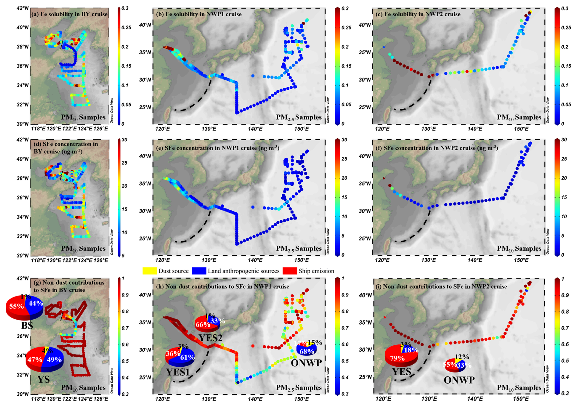
Figure 9 Iron solubility, soluble Fe concentration, and soluble Fe sources in three cruises. (a–c) Coloured dots represent atmospheric Fe solubility (dimensionless) for the BY cruise (PM₁₀ samples), NWP1 cruise (PM_2.5 samples), and NWP2 cruise (PM₁₀ samples), respectively. (d–f) Coloured dots represent atmospheric soluble Fe concentrations (ng m⁻³) for the three cruises. (g–i) Coloured dots represent the fractional contribution of non-dust sources to soluble Fe (dimensionless). Pie charts in (g)–(i) depict the average contributions of different sources to soluble Fe in different cruise legs (figures generated using Ocean Data View; Schlitzer, 2025).

The trend of higher contributions from non-dust sources to soluble Fe in coastal regions than in open ocean has also been captured by most models. However, the specific contribution values vary considerably among studies due to differences in emission inventories and atmospheric chemical processing schemes. For example, Wang et al. (2015) reported that non-dust sources (combustion-related) accounted for more than 95 % of soluble Fe deposition in Chinese marginal seas and over 85 % in the open Northwest Pacific. In comparison, Ito et al. (2019) simulated contributions exceeding 80 % and 70 % for these two regions, respectively. Lower estimates have also been reported, such as 40 %–60 % when considering anthropogenic sources alone (Matsui et al., 2018), and 20 %–60 % when anthropogenic and wildfire sources were combined (Rathod et al., 2020).

In addition to the zonal gradient, a pronounced meridional variation was also observed in the open Northwest Pacific. During the NWP1 cruise, the contribution of non-dust sources to atmospheric soluble Fe concentrations was lower in low-latitude regions. For PM_2.5 samples collected south of 26° N, the non-dust contribution averaged 49.5 % ± 10.8 % (Fig. 9h). Some models have reproduced such meridional variations in non-dust contributions (Lin et al., 2015; Wang et al., 2015), whereas others have shown little or no such pattern in this region (Matsui et al., 2018; Ito et al., 2019).

Both land anthropogenic emissions and ship emission exerted substantial influences on marine atmospheric soluble Fe. During the BY cruise, contributions from these two sources were comparable, with ship emission slightly exceeding land anthropogenic contributions in the Bohai Sea (Fig. 9g). In comparison, shipping contributions markedly exceeded those from land anthropogenic sources during the YES2 leg of the NWP1 cruise and the YES and ONWP legs of the NWP2 cruise (Fig. 9h and i). As these three legs took place in June–July, this may indicate that the contribution of ship emission to marine atmospheric soluble Fe increases markedly in summer. This pattern was probably attributable to the suppression of land-derived aerosols transport to the ocean by the East Asian Summer Monsoon (southwesterly to southerly winds), which in turn enhanced the relative contribution from local ship emission. In addition, Jiang et al. (2024) reported that metal emissions from ships in this region were higher in summer than in spring, which may also contribute to the observed seasonal variations. Collectively, these findings indicate that the sources of marine atmospheric soluble Fe exhibit not only spatial differences but also temporal variability.

3.3 Spatiotemporal variations of Fe sources

3.3.1 Spatial distribution of Fe concentration from different sources

Across all cruises, atmospheric total Fe concentrations generally ranged from 10 to 300 ng m⁻³ (10th–90th percentile: 10.17–300.4 ng m⁻³), while dust-derived Fe, identified via PMF analysis, ranged from 3 to 130 ng m⁻³ (10th–90th percentile: 2.61–128.4 ng m⁻³). Total Fe and dust-derived Fe exhibited broadly similar spatial patterns (Fig. 10a and c), with higher values in the Bohai and Yellow Seas, along with sporadic elevated values detected in open-ocean regions east and south of Japan. The highest levels occurred near the Shandong Peninsula during a major dust event (EP3, detailed in Sect. 3.1.3) during the BY cruise, when mean dust-derived Fe reached 801.5 ± 283.6 ng m⁻³, which was nearly 17 times the average of other samples (47.45 ± 67.04 ng m⁻³). Consequently, dust-derived Fe concentrations in the YS leg of the BY cruise were significantly higher than in other legs (Fig. 10d).

The comparisons of Fe concentration gradients between the Chinese marginal seas and the open Northwest Pacific during the same cruise showed that, during NWP1 cruise (PM_2.5 samples), the average concentrations of total Fe and dust-derived Fe over coastal waters were approximately 1.6 and 1.1 times higher, respectively, than those in the open ocean. These contrasts were less pronounced than model simulations. For example, Zhu et al. (2025) using the CAM model to simulate spring dust concentrations for 2015–2017, reported dust mass concentrations of 20–60 µg m⁻³ over the Bohai and Yellow Seas, markedly higher than the 5–20 µg m⁻³ over the open Northwest Pacific. The relatively weak gradient observed during the NWP1 cruise is likely attributable to the prevailing East Asian summer monsoon, which transported air masses over the sampling region from oceanic regions rather than the continent (Fig. S10a), thereby limiting dust input from East Asia.

In comparison, during NWP2 cruise (PM₁₀ samples), although air mass trajectories were also dominated by marine origins (Fig. S10b), the nearshore-offshore differences in both total Fe and dust-derived Fe were more pronounced than those during NWP1 cruise. This pattern was partly driven by enhanced coastal Fe concentrations associated with the larger aerosol size sampled in NWP2. During the YES leg of NWP2, total Fe in PM₁₀ reached 108.2 ± 248.3 ng m⁻³, exceeding those measured in PM_2.5 during the YES leg of NWP1 (76.35 ± 52.40 ng m⁻³). In contrast, over the open ocean, total Fe concentrations during NWP2 (23.30 ± 29.42 ng m⁻³) were lower than those in PM_2.5 during NWP1 (47.46 ± 50.57 ng m⁻³). This anomaly was likely driven by wet scavenging associated with precipitation. Substantial rainfall over the open Northwest Pacific south of Japan (130–144° E) during the NWP2 period (Fig. S11) likely removed atmospheric particles efficiently, resulting in extremely low Fe concentrations (7.81 ± 7.62 ng m⁻³) in this region. Such precipitation-induced wet scavenging over the open ocean further amplified the nearshore–offshore Fe gradient during NWP2.

During the three cruises, substantial amounts of land anthropogenic Fe were detected in the marine atmosphere, typically ranging from 1 to 100 ng m⁻³ (10th–90th percentile: 1.12–106.8 ng m⁻³). Compared with dust-derived Fe, land-anthropogenic Fe showed greater variability among cruises. As shown in Fig. 10e, concentrations during the BY cruise were significantly higher than those during the Northwest Pacific cruises. Similar to dust-derived Fe, occasional high concentrations were also observed over open-ocean regions. For example, during the NWP1 cruise, persistently elevated levels (66.19–104.5 ng m⁻³) were recorded southeast of Japan for approximately 32 h. These samples were notably enriched in pollution-related elements such as As, Zn, and Pb, reaching 4.5, 3.5, and 2.7 times the cruise averages, respectively, suggesting substantial influence from coal combustion and industrial emissions on land. Cruise-leg comparisons (Fig. 10f) show that land anthropogenic Fe concentrations were significantly higher in the Bohai Sea (72.34 ± 39.97 ng m⁻³) and Yellow Sea (75.70 ± 60.79 ng m⁻³) legs than in other legs. In both Northwest Pacific cruises, pronounced contrasts were observed between the coastal and open-ocean legs. During NWP1, the mean land anthropogenic Fe concentration in the YES leg was 3.0 times higher than that in the ONWP leg, and during NWP2 the difference increased to 4.7 times.

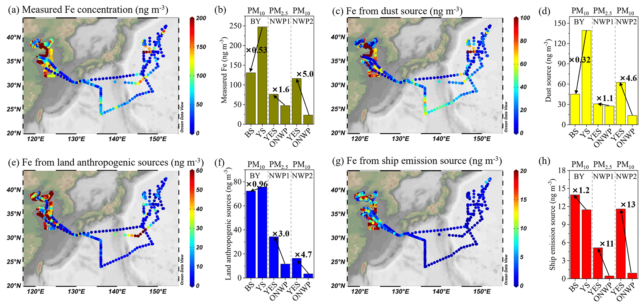
Figure 10 Spatial distribution of Fe concentrations from different sources. (a), (c), (e), (g) represent spatial distributions of measured total Fe, and PMF-resolved dust Fe, land anthropogenic Fe, and shipping Fe concentrations, respectively. (b), (d), (f), (h) represent mean concentrations of the corresponding Fe categories for different cruise legs, respectively; the three cruises are separated by dashed lines. Arrows and labels between bars indicate multiples of concentration differences between legs within the same cruise (figures generated using Ocean Data View; Schlitzer, 2025).

As shown in Fig. 10g, Fe concentrations from ship emission were generally much lower than those from other sources, typically below 20 ng m⁻³ (10th–90th percentile: 0.01–20.04 ng m⁻³). Unlike land-based dust and anthropogenic emissions, ship emission originates in marine areas and are primarily concentrated around ports and along major shipping routes (Chen et al., 2017; Johansson et al., 2017; Zhang et al., 2017). Consequently, the spatial variability in ship emission intensity over the ocean likely exerts a strong influence on the spatial distribution of ship-sourced Fe concentrations in marine aerosols. Source apportionment results from the three cruises indicate that elevated concentrations of shipping Fe were primarily observed in legs within the Chinese marginal seas (Fig. 10g), reflecting the high density of maritime traffic in these regions. The coastal sampling tracks in this study were located near more than a dozen major ports, including Dalian, Yingkou, Qinhuangdao, Tangshan, Tianjin, Huanghua, Yantai, Qingdao, Rizhao, Lianyungang, Nantong, and Shanghai (Chen et al., 2017). Ship emission in these port areas, as well as along the shipping lanes connecting them, contributed substantially to ship-sourced Fe, resulting in generally high concentrations in coastal legs. Mean ship-sourced Fe concentrations across different legs in marginal seas ranged from 5.15 ng m⁻³ in PM_2.5 samples to 13.95 ng m⁻³ in PM₁₀ samples (Fig. 10h). These values were higher than those simulated by Jiang et al. (2024) using the CMAQ model, which estimated ship-sourced Fe concentrations in the Bohai and Yellow Seas at around 3 ng m⁻³, with high-concentration zones exceeding 6 ng m⁻³. However, the average concentrations observed in our two open-ocean legs (0.46 and 0.92 ng m⁻³) were comparable to Jiang's simulation results for these regions, which were generally below 1 ng m⁻³.

Compared to dust-derived and land anthropogenic Fe, ship-sourced Fe exhibited a much sharper nearshore-offshore gradient. As shown in Fig. 10h, during NWP1 cruise and NWP2 cruise, the YES legs exhibited ship-sourced Fe concentrations up to 11 and 13 times higher, respectively, than those in the corresponding open-ocean legs. This pattern was consistent with spatial differences in ship emission intensities. For example, the ship emission inventory of Johansson et al. (2017) indicates that PM_2.5 emissions from ships in the Chinese marginal seas were several tens of times higher than those in the open Northwest Pacific east of Japan.

3.3.2 Spatiotemporal variations of atmospheric total Fe and soluble Fe sources

The differing spatial patterns of Fe concentrations from various sources lead to marked spatial variability in the source structure of Fe in marine aerosols. The source structure of atmospheric total Fe in individual samples is shown in Fig. 11a. Most samples are distributed between the vertices representing land anthropogenic sources and dust source, indicating that these two sources were the dominant contributors to total Fe during the observation period. Samples from the open Northwest Pacific generally plot closer to the dust-source vertex, both for PM₁₀ samples in NWP2 cruise and PM_2.5 samples in NWP1 cruise. Most of these samples fall to the right of the yellow diagonal line in Fig. 11a, indicating a dust contribution exceeding 50 %. In contrast, ship emission contributions to total Fe were generally low (<25 %). Samples with ship source contributions above 25 % were mainly collected in coastal regions. Notably, among the 11 samples with ship contributions exceeding 50 % (to the left of the red diagonal line in Fig. 11a), seven were collected in coastal seas during the summer NWP2 cruise, highlighting the elevated role of ship emission in coastal regions during summer.

In comparison, Fig. 11b illustrates the source structure of atmospheric soluble Fe in individual samples. Most sample points are located between the vertices representing land anthropogenic sources and ship emission, indicating that soluble Fe during the observation period was primarily derived from non-dust sources. Samples with dust-source contributions exceeding 25 % were primarily PM_2.5 samples collected during the NWP1 cruise over the open Northwest Pacific, with a few additional PM₁₀ samples collected during the BY cruise and the open ocean segment of NWP2 cruise.

The average source structure of total Fe and soluble Fe for each cruise leg is shown in Fig. 11c and d. Overall, dust remained the dominant source of total Fe, accounting for 59 %–76 % in three PM₁₀-sampling cruise legs (BY, coastal NWP2, and open NWP2) and 44 %–70 % in two PM_2.5-sampling cruise legs (coastal and open NWP1). For both size fractions, dust contributions were higher in the open Northwest Pacific (≥70 %) than in coastal sea regions. These results are generally comparable to recent Fe source analysis (based on PMF) in Qingdao, a coastal city in the Yellow Sea, where dust (including fresh and aged dust) accounted for 71 % of total Fe in spring PM_2.5 samples (Li et al., 2025a) and 46 %–80 % in coarse particles (PM_>1) across seasons (Chen et al., 2024).

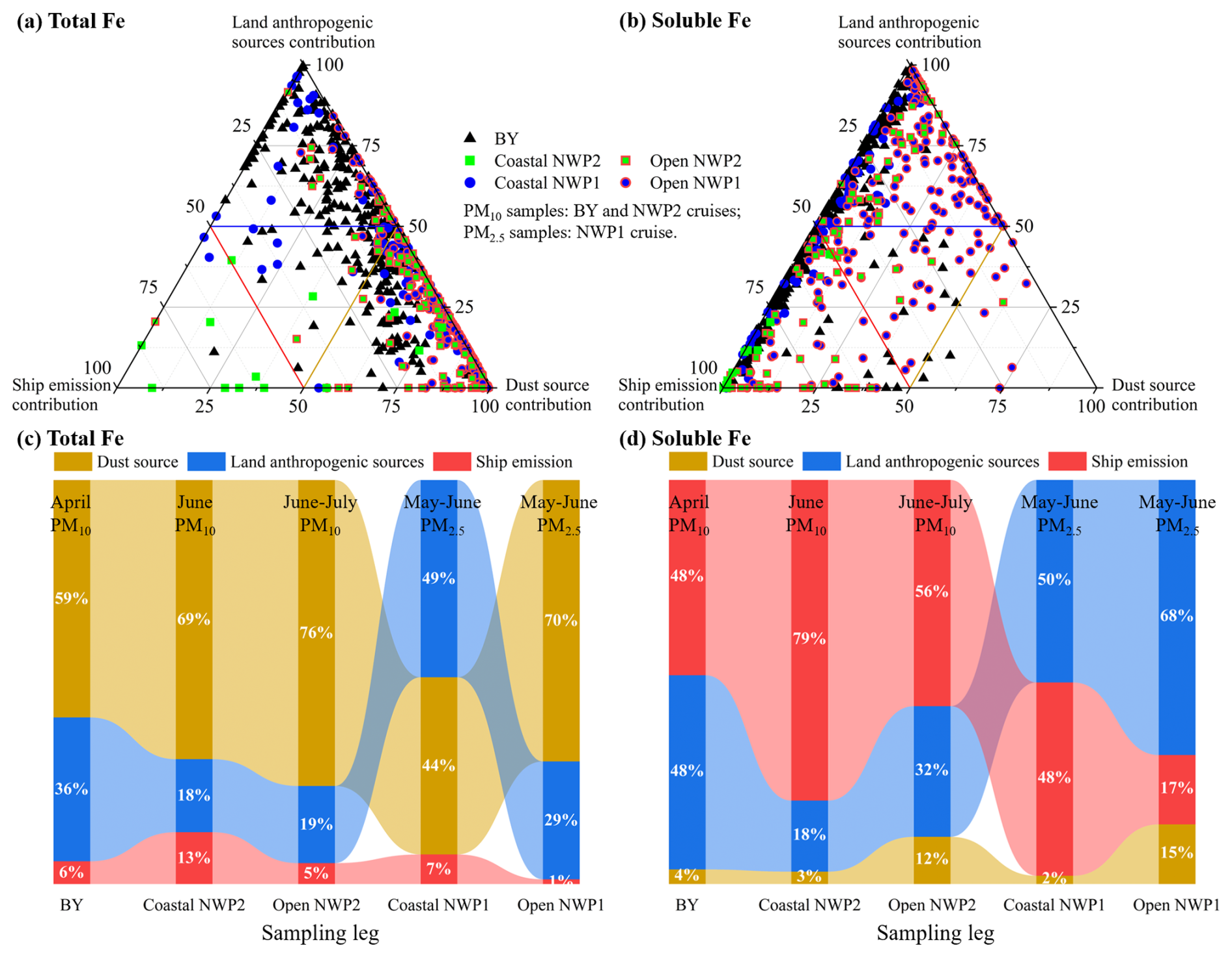
Figure 11 Source structure of total Fe and soluble Fe across different cruises and sea areas. (a) and (b) are ternary plots illustrating the source structure of total Fe and soluble Fe, respectively; the three vertices represent the three sources; the closer a sample point is to a given vertex, the greater the relative contribution of that source to the sample. (c) and (d) show the average contributions of the three sources to total Fe and soluble Fe, respectively, across different sampling legs. BY refers to all samples collected during the BY cruise. Coastal NWP2 (or NWP1) represents samples collected from coastal regions, including the Yellow Sea and East China Sea, during the NWP2 (or NWP1) cruise, while Open NWP2 (or NWP1) refers to samples collected from the open Northwest Pacific.

However, non-dust sources, including land anthropogenic sources and ship emission, dominated atmospheric soluble Fe consistently in this study, with contributions to soluble Fe reaching 88 %–97 % in three PM₁₀-sampling cruise legs and 85 %–98 % in two PM_2.5-sampling cruise legs. These results were comparable with previous PMF-based studies in coastal cities (Chen et al., 2024; Li et al., 2025a), but were notably higher than recent Fe isotope–based estimates. For example, Hsieh and Ho (2024) reported 35 %–99 % anthropogenic contribution to soluble Fe in the 0.57–1.0 µm size fraction (ammonium acetate buffer leach) at Pengjia Island, while Kurisu et al. (2024) found 0 %–45 % in bulk aerosols (ultrapure water leach) over the North Pacific. Isotope-based source apportionment is highly sensitive to end-member selection. Bunnell et al. (2025) showed that using two different anthropogenic Fe isotope end-members could result in nearly a threefold difference in the inferred anthropogenic contribution to soluble Fe over the North Pacific. This sensitivity and the associated uncertainties may limit the quantitative comparability of isotope-based estimates with PMF-derived results.

Among non-dust sources, land anthropogenic sources were important contributors to both total Fe and soluble Fe, with relatively higher contributions to PM_2.5 samples than to PM₁₀ samples (Fig. 11c and d). For PM_2.5 samples in coastal NWP1 (May–June), the contribution to total Fe (49 %) is comparable to that reported by Qi et al. (2025) during coastal cruise in spring (44.5 % for total Fe in PM_2.5), but lower than their coastal cruise in summer (80.5 %). For PM_2.5 samples in open NWP1, land anthropogenic sources contributed 29 % to total Fe and 68 % to soluble Fe, which are slightly lower than our previous observations of Fe in PM_2.5 in the open Northwest Pacific during spring 2015 (36 % and 77 %, respectively) (Zhang et al., 2024).

Compared with land anthropogenic sources, ship emission contributed much less to total Fe, but their contribution to soluble Fe was substantial, particularly in the three coastal cruise legs (BY, Coastal NWP2, and Coastal NWP1), ranging from 48 % to 79 %, and peaking in summer (Coastal NWP2, 79 %). The predominance of ship emission as the main source of soluble Fe in coastal regions during summer can be attributed to two main factors. First, intensive shipping activity in Chinese marginal seas results in relatively high absolute concentrations of ship-derived Fe (Fig. 10g). Second, increased precipitation during summer suppresses dust emissions, and the East Asian summer monsoon reduces the transport of aerosols from land to sea. For example, Ito (2013) reported that under low Asian dust conditions, ship emission could account for up to 40 % of soluble Fe deposition over the Northeast Pacific in summer based on model simulations. Based on observations from the eastern coastal region of South Korea, Seo and Kim (2023) found that ship emissions contributed as much as 45 % of atmospheric soluble Fe concentration.

Given the significant reductions in land anthropogenic emissions and coastal ship emission resulting from China's recent air pollution control policies (Dong et al., 2025; Zhang et al., 2025), along with the interannual variability of dust activity (Tai et al., 2021; Zhu et al., 2025), the future source structure of atmospheric total Fe and soluble Fe over the ocean remains uncertain. Therefore, more observations, particularly from shipborne measurements, are essential for improving our understanding of real-world changes in the marine atmosphere. Such data are also critical for optimizing atmospheric models and providing accurate inputs to ocean biogeochemical models to assess the environmental impacts of atmospheric composition changes.

4 Summary and conclusions

This study provides a comprehensive assessment of the sources and spatiotemporal variability of atmospheric Fe over the Chinese marginal seas and the open Northwest Pacific Ocean, based on shipborne high-time-resolution measurements from three observation campaigns. Our results demonstrate that dust remains the most important contributor to total Fe, particularly in the open ocean, whereas non-dust sources (including land anthropogenic sources and ship emission) are the primary contributors to soluble Fe, especially in coastal regions. Among non-dust sources, land anthropogenic sources contributed substantially to both total Fe and soluble Fe, with its highest contributions being 49 % to total Fe in coastal PM_2.5 and 68 % to soluble Fe in open Northwest Pacific PM_2.5, both were observed during the NWP1 cruise. In contrast, the contribution of ship emission to total Fe was relatively minor, yet it was a notable source of soluble Fe, reaching a mean contribution of 79 % in coastal PM₁₀ samples during the NWP2 cruise. Additionally, non-dust Fe concentrations exhibited stronger spatial variability than dust-derived Fe. For instance, the average concentration of land anthropogenic Fe in the Chinese marginal seas was 3–5 times higher than in the open Northwest Pacific during the same cruises, and shipping Fe showed even greater contrasts, with coastal concentrations exceeding open Northwest Pacific values by more than an order of magnitude.

Methodologically, this study validated and advanced approaches for atmospheric Fe source apportionment in marine environment. By comparing PMF-resolved source-specific total Fe derived from online measurements with traditional filter-based chemical tracers, we confirmed the utility of Al as a reliable tracer for dust-derived Fe in marine atmosphere, particularly during intense dust events. However, our results also highlight that dust input can interfere with the source attribution of tracers for non-dust sources by increasing their concentrations, particularly evident for V, and to a lesser extent for Pb. We further estimated Fe solubility and apportioned soluble Fe sources using empirical solubility factors assigned to different sources. These estimates showed strong agreement with laboratory-based solubility measurements from filter samples (R²=0.84), supporting the robustness of the proposed parameterization approach. In addition, comparison with previous modeling studies suggests that some models may underestimate the high solubility of Fe in the Northwest Pacific and may have limitations in capturing the meridional variation of soluble Fe sources in this region.

Overall, the findings highlight the important role of non-dust sources in shaping the bioavailable Fe pool in the marine atmosphere, both from anthropogenic activities on land and oceanic regions (ship emission). The distinct spatial and seasonal variations in Fe sources revealed in this study provide valuable observational constraints for improving Fe deposition models, and offer new insights into the biogeochemical impacts of land anthropogenic and ship emission on marine ecosystems.