Cross-Seasonal Impact of SST Anomalies over the Tropical Central Pacific Ocean on the Antarctic Stratosphere

In this study we examine the cross–seasonal effects of boreal winter sea surface temperature (SST) anomalies over the tropical central Pacific (Niño 4 region) on Antarctic stratospheric circulation and ozone transport during the subsequent austral winter using ERA5 reanalysis of 45 years (1980–2024). Our analyses show that warm (cold) SST anomalies in the Niño 4 region during December–February are associated with mid- and high-latitude stratospheric warming (cooling), a contracted (expanded) stratospheric polar vortex (SPV), and enhanced (suppressed) polar ozone concentrations in the subsequent July–September period. This delayed response is mediated by the Pacific–South America (PSA) teleconnection pattern, which excites planetary waves that propagate upward into the stratosphere, thereby modifying the Brewer–Dobson circulation and enhancing ozone poleward transport, ultimately warming polar stratosphere. In addition, as the influence of the Niño 4 SST anomalies on the PSA teleconnection pattern diminishes during July–September, surface heat feedback at mid- and high-latitude becomes critically important for planetary waves. For example, persistent southeastern Pacific SST warming and sea–ice loss over the Amundsen and Ross Seas reinforce planetary waves by releasing heat from ocean into atmosphere. A multivariate regression statistical model using factors of boreal winter Niño 4 SST and June PSA indices explains approximately 32 % of the variance in austral winter stratospheric temperatures. These findings highlight a previously underexplored pathway through which tropical Pacific SST anomalies modulate Antarctic stratospheric dynamics on cross-seasonal timescales.

1 Introduction

The Antarctic stratospheric circulation is largely governed by the wintertime Stratospheric Polar Vortex (SPV), which is a major driver of weather and climate variability across the Southern Hemisphere (Baldwin et al., 2021). Compared to its Northern Hemisphere counterpart, the Antarctic SPV is generally more stable, owing to weaker thermal contrasts between the ocean and land. Despite this stability, the Antarctic SPV exhibits considerable interannual variability (Domeisen et al., 2019; Baldwin et al., 2021). Therefore, the Antarctic stratosphere plays a crucial role in modulating weather and climate in the Southern Hemisphere through the seasonal evolution of SPV and its dynamics processes and interaction with ozone chemistry (Thompson et al., 2005; Solomon et al., 2016).

Previous studies revealed large interannual variations and long-term trends in the SPV, stratospheric temperatures, and ozone concentrations (Karpetchko et al., 2005; Hu et al., 2022). Superimposed on the long-term trends of SPV are substantial interannual variations and extreme events (Shen et al., 2020; Zi et al., 2025; Lim et al., 2026). For instance, exceptionally weak SPV episodes triggered by sudden stratospheric warmings (SSWs) occurred respectively in 2002, 2010, 2019, and 2024 (Thompson and Solomon, 2002; Esler et al., 2006; Laat and Weele 2011; Shen et al., 2020; Zi et al., 2025; Lim et al., 2026), and an unusually strong SPV event driven by the pronounced ozone depletion occurred in 2020 (Lim et al., 2024).

Several natural factors contribute to the above-mentioned SPV variability. The phase of the Quasi–Biennial Oscillation (QBO), for instance, modulates planetary wave propagation and can either strengthen or weaken the SPV (Kuroda et al., 2007). El Niño–Southern Oscillation (ENSO) events also leave distinct warm- and cold-year signatures on Antarctic stratospheric temperatures through changes in tropospheric wave forcing and the Brewer–Dobson (B–D) circulation (Yang et al., 2015; Stone et al., 2022; Rao et al., 2023; Wang et al., 2025). Previous studies also suggest sea–ice can have significant impact on the SPV (Rea et al., 2024; Song et al., 2025; Sun et al., 2015), with implications for Southern Hemisphere climate variability. In addition, solar-cycle variability contributes to interannual modulation by altering ultraviolet irradiance and stratospheric heating rates (Kuroda et al., 2007). Alongside these natural drivers, fluctuations in the atmospheric burdens of ozone-depleting substances and greenhouse gases continue to influence both the magnitude and nature of Antarctic stratospheric variability (Singh and Bhargawa, 2019).

ENSO is the most prominent mode of interannual climate variability (Wang, 2018). Developing in boreal autumn and peaking in winter, ENSO influences the global weather patterns through atmospheric teleconnections (McPhaden et al., 2006). It also modulates the SPV primarily via the Pacific–North America (PNA) and the Pacific–South America (PSA) wave trains (Garfinkel and Hartmann, 2008; Ineson and Scaife, 2009; Barriopedro and Calvo, 2014; Polvani et al., 2017; Song and Son, 2018; Zhang et al., 2022). In the Northern Hemisphere, El Niño events enhance tropical convection and amplify the PNA pattern, strengthening the Aleutian Low, which in turn increases upward wave activity and weakens the SPV (Garfinkel and Hartmann, 2008; Butler and Polvani, 2011; Zhang et al., 2022). In the Southern Hemisphere, central Pacific (CP-type) El Niño events during September–February enhance convection near the South Pacific Convergence Zone (SPCZ), which triggers the PSA wave trains that can weaken the Antarctic SPV, resulting in polar stratospheric warming and enhanced ozone concentration (Hurwitz et al., 2011a, b; Yang et al., 2015; Manatsa and Mukwada, 2017; Domeisen et al., 2019; Ma et al., 2022). In contrast, Eastern Pacific (EP-type) El Niño events have been found to produce weaker Antarctic stratospheric responses (Hurwitz et al., 2011a; Zubiaurre and Calvo, 2012).

Although many studies have examined the Antarctic stratosphere's simultaneous or 1–2 months lagged responses to ENSO from September to February of following year (L'Heureux and Thompson, 2006; Silvestri and Vera, 2009; Hu and Fu, 2010; Fogt et al., 2011; Lin et al., 2012; Kim et al., 2017; Ma et al., 2022), our knowledge remains very limited on the ENSO's cross-seasonal and delayed effects (Manatsa and Mukwada, 2017; Niu et al., 2023). Some previous studies have found that delayed ozone responses occur in the year following an ENSO event (Lin and Qian, 2019), while others have suggested that tropical sea surface temperature (SST) anomalies as early as June can influence stratospheric circulation later in the year (Grassi et al., 2008; Evtushevsky et al., 2015; Lim et al., 2018; Stone et al., 2022). Yang et al. (2015) examined correlations between ENSO and Antarctic stratospheric temperatures during July–September, but these were primarily interpreted as concurrent responses. Despite these studies, the physical mechanisms by which ENSO events in boreal winter influence the Antarctic stratosphere during the following austral winter (July–September) remain poorly understood. During the austral winter, the SPV reaches its maximum strength and is also particularly susceptible to dynamical disturbances. Consequently, a deeper understanding of the delayed impacts of El Niño is crucial for improving prediction of Antarctic stratospheric extreme events (Lin et al., 2009; Thompson et al., 2011).

The primary objective of this study is to examine how the boreal winter tropical central Pacific SST anomalies (SSTa) influence the Antarctic stratosphere during the following austral winter, with particular emphasis on the mechanisms through which tropical central Pacific SSTa modulate Antarctic stratospheric dynamics, and associated planetary wave propagation and mid-latitude sea–air interactions. The structure of this paper is as follows. Section 2 describes the data and methodology; Sect. 3 quantifies the relationship between the tropical central Pacific SST and Antarctic stratosphere; Sect. 4 examines the underlying dynamical mechanisms; Sect. 5 presents the multivariate regression analysis; Sect. 6 evaluates CMIP6 model validation; Sect. 7 provides a summary and conclusion.

2 Data and methods

2.1 Data

The 6 hourly and monthly-mean atmospheric variables over the 45-year period (1980–2024) extracted from the ERA5 reanalysis (Hersbach et al., 2023a, b) are used in this study. This reanalysis with a horizontal resolution of 1°×1° was generated by the European Centre for Medium-Range Weather Forecasts (ECMWF). These atmospheric variables include the geopotential height, horizontal and vertical winds, temperature and ozone mass mixing ratio with 37 vertical pressure levels; sea level pressure (SLP), total column ozone (TCO₃), net surface downward short-wave radiation flux, net surface upward long-wave radiation flux, latent and sensible heat fluxes, outgoing long-wave radiation flux (OLR) with single level. The monthly sea surface temperature (SST) and sea–ice concentration (SIC) during the same study period were also extracted from ERA5 reanalysis.

Several indices (such as Niño 3, Niño 3.4, and Niño 4) based on SST anomalies averaged over a given region have been used to monitor the dynamic activities in the tropic Pacific (Bamston et al., 1997; Trenberth, 1997). The Niño 3 index represents the SST anomalies averaged over 5° N–5° S and 150–90° W, and is used for monitoring and predicting El Niño and La Niña events (Trenberth, 1997). The Niño 3.4 index is the SST anomalies averaged over 5° N–5° S and 170–120° W, and is used as the primary index for monitoring ENSO due to its ability to capture basin-scale variability (Bamston et al., 1997). The Niño 4 index is the SST anomalies averaged over 5° N–5° S and 160° E–150° W, which is used to monitor SST anomalies in the tropical central Pacific. In this study, the SST indices for Niño 3, Niño 3.4, and Niño 4 were obtained from the HadISST1.1 dataset (Rayner et al., 2003).

The Pacific–South America pattern (PSA) index is used to examine stratosphere and troposphere interactions, and is derived by projecting area-weighted SLP anomalies south of 20° S onto the second Empirical Orthogonal Function (EOF) mode (Mo and Higgins, 1998). All anomalies are calculated relative to the 1991–2020 daily and monthly climatology, and all data have been detrended. Since results obtained after filtering the decadal component are similar, no filtering has been applied. Statistical significance is assessed using the Student's t test.

2.2 Method

2.2.1 Eliassen–Palm flux

The Eliassen–Palm (E–P) flux is used to diagnose interactions between eddies and the zonal–mean flow in both the stratosphere and troposphere (Andrews et al., 1987). The E–P flux (F) and its divergence (∇⋅F) are defined as:

$$\begin{array}{}\text{(1)}& {\displaystyle }\mathit{F}=({\mathit{F}}_{\mathit{\phi }},{\mathit{F}}_{\mathrm{p}})=r_{\mathrm{0}}\cos \mathit{\phi }\left\{-\left[u^{\prime }{v}^{\prime }\right],{\displaystyle \frac{f}{\left[{\mathit{\theta }}_{\mathrm{p}}\right]}}\left[v^{\prime }{\mathit{\theta }}^{\prime }\right]\right\},\text{(2)}& {\displaystyle }\mathrm{\nabla }\cdot \mathit{F}={\displaystyle \frac{\mathrm{1}}{r_{\mathrm{0}}\cos \mathit{\phi }}}{\displaystyle \frac{\partial }{\partial \mathit{\phi }}}\left({\mathit{F}}_{\mathit{\phi }}\cos \mathit{\phi }\right)+{\displaystyle \frac{\partial }{\partial p}}\left({\mathit{F}}_{\mathrm{p}}\right),\end{array}$$

where u and v are the zonal and meridional wind components, respectively, and θ is the potential temperature. φ and p denote latitude and pressure, respectively. f is the Coriolis parameter, and r₀ is Earth's radius. Square brackets [ ] indicate zonal averages, and primes (′) denote deviations from the zonal mean.

2.2.2 Takaya–Nakamura wave activity flux

The Takaya–Nakamura (2001) wave activity flux (TN01 flux) is used to determine the horizontal propagation of quasi-stationary Rossby waves in a zonally varying background flow (Takaya and Nakamura, 2001). The zonal (F_x) and meridional (F_y) components of TN01 are defined as:

$$\begin{array}{}\text{(3)}& {\displaystyle }\begin{array}{rl}{F}_x=& {\displaystyle \frac{p}{\mathrm{2}\left|U^{\times }\right|r_{\mathrm{0}}^{\mathrm{2}}}}\left({\displaystyle \frac{U}{\cos \mathit{\phi }}}\left({\left({\displaystyle \frac{\partial {\mathit{\psi }}^{\prime }}{\partial \mathit{\lambda }}}\right)}^{\mathrm{2}}-{\mathit{\psi }}^{\prime }{\displaystyle \frac{{\partial }^{\mathrm{2}}{\mathit{\psi }}^{\prime }}{\partial {\mathit{\lambda }}^{\mathrm{2}}}}\right)\right.\\ & \left.+V\left({\displaystyle \frac{\partial {\mathit{\psi }}^{\prime }}{\partial \mathit{\lambda }}}{\displaystyle \frac{\partial {\mathit{\psi }}^{\prime }}{\partial \mathit{\phi }}}-{\mathit{\psi }}^{\prime }{\displaystyle \frac{{\partial }^{\mathrm{2}}{\mathit{\psi }}^{\prime }}{\partial \mathit{\lambda }\partial \mathit{\phi }}}\right)\right)\end{array},\text{(4)}& {\displaystyle }\begin{array}{rl}{F}_y=& {\displaystyle \frac{p}{\mathrm{2}\left|U^{\times }\right|r_{\mathrm{0}}^{\mathrm{2}}}}\left(U\left({\displaystyle \frac{\partial {\mathit{\psi }}^{\prime }}{\partial \mathit{\lambda }}}{\displaystyle \frac{\partial {\mathit{\psi }}^{\prime }}{\partial \mathit{\phi }}}-{\mathit{\psi }}^{\prime }{\displaystyle \frac{{\partial }^{\mathrm{2}}{\mathit{\psi }}^{\prime }}{\partial \mathit{\lambda }\partial \mathit{\phi }}}\right)\right.\\ & \left.+V\cos \mathit{\phi }\left({\left({\displaystyle \frac{\partial {\mathit{\psi }}^{\prime }}{\partial \mathit{\phi }}}\right)}^{\mathrm{2}}-{\mathit{\psi }}^{\prime }{\displaystyle \frac{{\partial }^{\mathrm{2}}{\mathit{\psi }}^{\prime }}{\partial {\mathit{\phi }}^{\mathrm{2}}}}\right)\right),\end{array}\end{array}$$

where ψ represents the stream function, λ and φ denote longitude and latitude, respectively, and $\left|U^{\times }\right|$ is the magnitude of the total horizontal wind velocity. U and V are the climatological mean zonal and meridional wind components, respectively, while p is pressure, and r₀ is Earth's radius.

2.2.3 Residual mean meridional circulation

The Transformed Eulerian-Mean (TEM) formulation proposed by Andrews and McIntyre (1976, 1978) has widely been used to diagnose large-scale circulation in the middle atmosphere. Unlike the conventional Eulerian mean, the TEM framework accounts for eddy heat and momentum fluxes, thereby providing a more accurate representation of actual mass transport. In particular, the residual mean meridional circulation captures the net effect of both mean flow and wave-induced eddy motions, making it especially useful for diagnosing stratospheric processes, such as B–D circulation and wave-driven anomalies associated with stratospheric warming. It is defined as:

$$\begin{array}{}\text{(5)}& {\displaystyle }[v{]}^{\ast }=[v]-{\displaystyle \frac{\mathrm{1}}{{\mathit{\rho }}_{\mathrm{0}}}}{\displaystyle \frac{\partial }{\partial z}}\left({\displaystyle \frac{{\mathit{\rho }}_{\mathrm{0}}\left[v^{\prime }{\mathit{\theta }}^{\prime }\right]}{\left[{\mathit{\theta }}_z\right]}}\right),\text{(6)}& {\displaystyle }[w{]}^{\ast }=[w]-{\displaystyle \frac{\mathrm{1}}{r_{\mathrm{0}}\cos \mathit{\phi }}}{\displaystyle \frac{\partial }{\partial \mathit{\phi }}}\left({\displaystyle \frac{\cos \mathit{\phi }\left[v^{\prime }{\mathit{\theta }}^{\prime }\right]}{\left[{\mathit{\theta }}_z\right]}}\right),\end{array}$$

where [v]^∗ and [w]^∗ denote the meridional and vertical components of the residual velocity, respectively. The vertical coordinate z is the log-pressure height defined as z = $-H\log \frac{p}{\mathrm{1000}\mathrm{hPa}}$, where H is the scale height (≈ 7 km). All other variables are consistent with those defined in Eqs. (1)–(4).

2.2.4 Quasi-geostrophic wave refraction index

The quasi-geostrophic wave refraction index (n²) is also used to diagnose the propagation characteristics of planetary waves (O'Neill and Youngblut, 1982). In general, planetary waves tend to propagate toward regions with a larger value of the refraction index. The formula is given as follows:

$$\begin{array}{}\text{(7)}& n^{\mathrm{2}}=\left[{\displaystyle \frac{{\stackrel{\mathrm{‾}}{q}}_{\mathit{\phi }}}{r_{\mathrm{0}}(\stackrel{\mathrm{‾}}{u}-c)}}-{\left({\displaystyle \frac{k}{r_{\mathrm{0}}\cos \mathit{\phi }}}\right)}^{\mathrm{2}}-{\left({\displaystyle \frac{f}{\mathrm{2}NH}}\right)}^{\mathrm{2}}\right]r_{\mathrm{0}}^{\mathrm{2}},\end{array}$$

where the meridional gradient of the zonal mean potential vorticity ${\stackrel{\mathrm{‾}}{q}}_{\mathit{\phi }}$ is (Albers and Birner, 2014):

$$\begin{array}{}\text{(8)}& {\stackrel{\mathrm{‾}}{q}}_{\mathit{\phi }}=\mathrm{2}\mathrm{\Omega }\cos \mathit{\phi }-{\left[{\displaystyle \frac{(\stackrel{\mathrm{‾}}{u}\cos \mathit{\phi }{)}_{\mathit{\phi }}}{r_{\mathrm{0}}\cos \mathit{\phi }}}\right]}_{\mathit{\phi }}+{\displaystyle \frac{r_{\mathrm{0}}{f}^{\mathrm{2}}}{R_{\mathrm{d}}}}{\left({\displaystyle \frac{p\mathit{\theta }}{T}}{\displaystyle \frac{\stackrel{\mathrm{‾}}{u_{\mathrm{p}}}}{\stackrel{\mathrm{‾}}{{\mathit{\theta }}_{\mathrm{p}}}}}\right)}_{\mathrm{p}},\end{array}$$

where u is the zonal-mean zonal wind; NH, k, f, φ, r₀ and Ω are the buoyancy frequency, scale height, zonal wave number, the Coriolis parameter, latitude, Earth's radius and angular frequency of Earth, respectively. The subscripts indicate derivatives with respect to the corresponding variables (φ and p) and the prime denotes deviation from the zonal mean.

2.2.5 CMIP6 datasets

To validate the observational results against model simulations, output from Phase 6 of the Coupled Model Intercomparison Project (CMIP6) are examined. Historical simulations were performed using fully coupled sea–air models forced with observed external drivers, including greenhouse gases, aerosols, volcanic eruptions, and solar variability. The analysis focuses on monthly mean SST, SIC, and temperature at 10 hPa over the period 1950–2014. A total of 24 fully coupled CMIP6 models are included: CESM2, CESM2-FV2, CESM2-WACCM, CESM2-WACCM-FV2, E3SM-1-0, E3SM-1-1, E3SM-2-0, E3SM-2-1, CanESM5, CanESM5-1, HadGEM3-GC31-LL, HadGEM3-GC31-MM, CNRM-CM6-1, CNRM-ESM2-1, EC-Earth3-Veg, EC-Earth3-AerChem, ACCESS-CM2, BCC-CSM2-MR, CAS-ESM2-0, FIO-ESM-2-0, IPSL-CM6A-LR, NESM3, MRI-ESM2-0, and MPI-ESM-1-2-HAM. Because the selected CMIP6 models differ in their horizontal resolutions, all fields are interpolated onto a uniform 1°×1° latitude–longitude grid to ensure consistency across datasets.

3 Impacts of SST anomalies on stratospheric atmospheric circulation

To quantify the cross-seasonal response of the Antarctic stratospheric circulation to tropical Pacific SST anomalies, we first correlate three ENSO indices: Niño 4, Niño 3.4, and Niño 3, with the stratospheric temperature (T₁₀₋₃₀) and zonal wind (U₁₀₋₃₀) over Antarctica during the subsequent July–September period. Here, T₁₀₋₃₀ refers to the zonal-mean temperature averaged over 60–90° S at 10–30 hPa, and U₁₀₋₃₀ refers to the zonal-mean zonal wind averaged over 40–50° S at the same pressure levels (Table 1).

Table 1 Correlation coefficients between the Niño 4, Niño 3.4 and Niño 3 indices and the zonal-mean temperature index (T₁₀₋₃₀) averaged over 60–90° S as well as the zonal wind index (U₁₀₋₃₀) averaged over 40–50° S at 10–30 hPa.

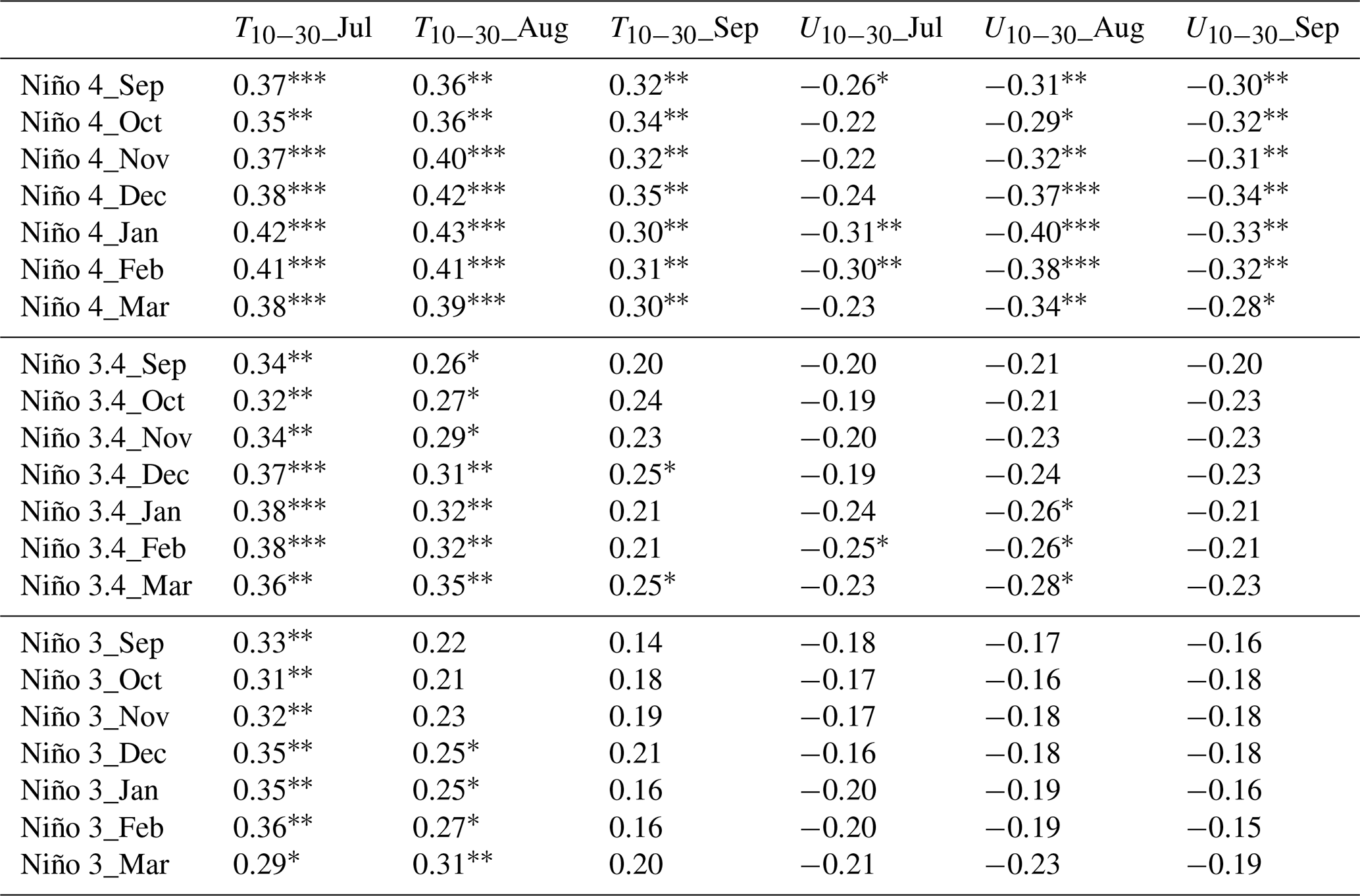
Note: asterisks indicate statistical significance: ${}^{***}$ represent 99 % confidence level, ${}^{**}$ for 95 %, and ^* for 90 %.

Among the three indices, the Niño 4 index shows the strongest correlation with Antarctic stratospheric circulations (Table 1). In particular, the Niño 4 index exhibits a significant positive correlation (R≥0.30, p<0.05) with the subsequent July–September T₁₀₋₃₀ index, with correlations from September–March reaching the 95 % confidence level. The largest correlation occurs during the boreal winter (December–February), with the January Niño 4 index showing the highest correlation with August T₁₀₋₃₀ (R=0.43, p<0.01). Additionally, the December–February Niño 4 index is significantly negatively correlated with the July–September U₁₀₋₃₀ index, with the strongest negative correlation between the January Niño 4 and August U₁₀₋₃₀ ($R=-\mathrm{0.40}$, p<0.01). These correlations are consistent with stratospheric warming (cooling) and a weakened (strong) Stratospheric polar vortex (SPV) associated with warm (cold) SSTa in the tropical central Pacific.

In comparison with the Niño 4 index, the Niño 3.4 index shows weaker correlations with stratospheric temperature and zonal wind. The January and February Niño 3.4 indices have the highest correlation with July T₁₀₋₃₀ (R=0.38, p<0.01), while the correlation with September T₁₀₋₃₀ is not statistically significant. Similarly, its correlation with U₁₀₋₃₀ is weak, with only a marginally significant negative correlation between the January–March Niño 3.4 index and August U₁₀₋₃₀ at the 90 % confidence level. However, the Niño 3 index exhibits the weakest correlations with polar stratospheric temperature and zonal wind. While a moderate correlation with T₁₀₋₃₀ is observed during July–August, correlations in September are very weak and do not exceed the 90 % significance threshold.

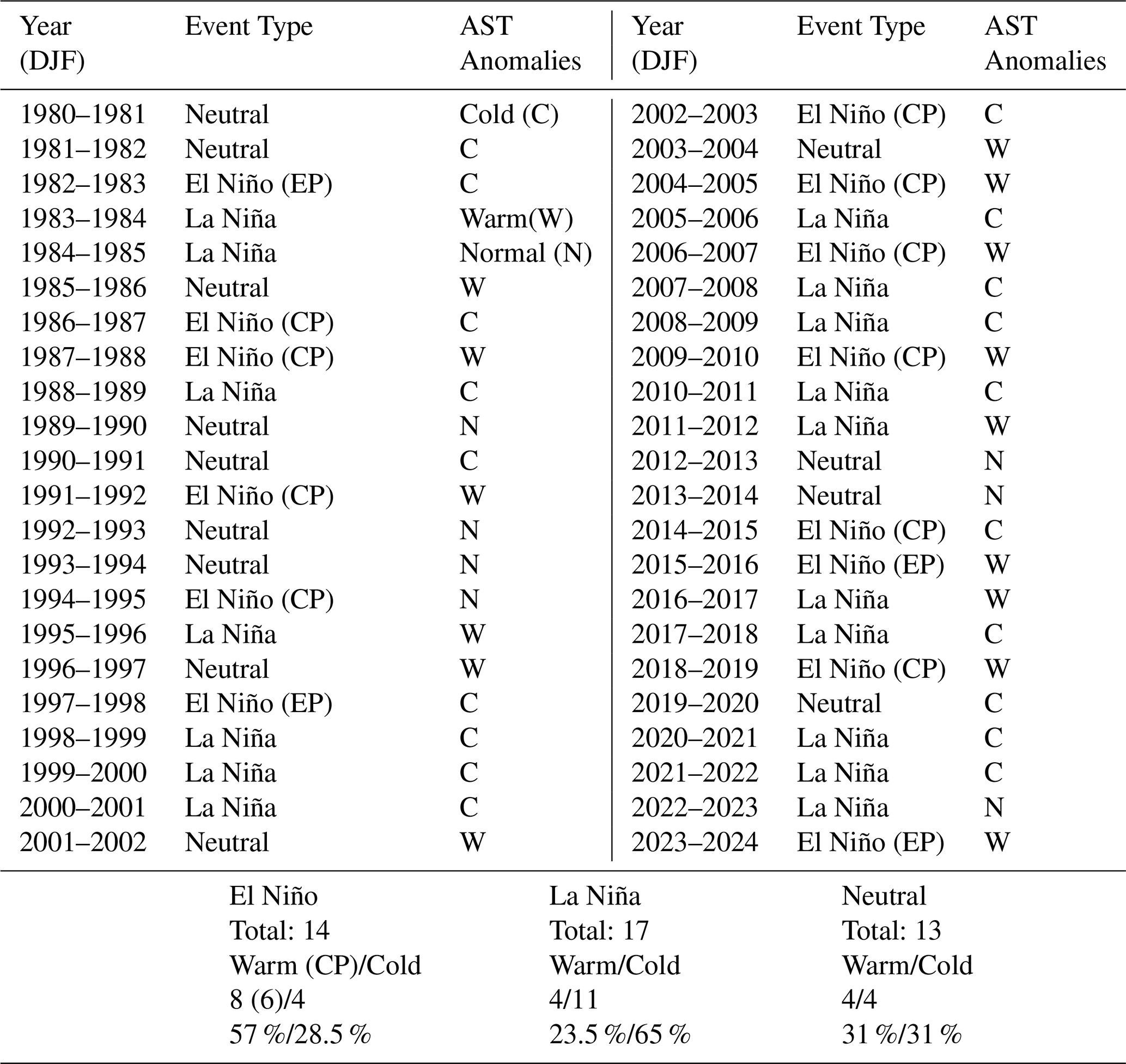
We next examine the relationship between ENSO phases in the preceding boreal winter and the Antarctic stratospheric circulation anomalies in July–September over the 45-year period 1980–2024 (Table 2). A warm (cold) stratospheric year is defined as one in which the July–September mean T₁₀₋₃₀ index is ≥0.5 ($\le -\mathrm{0.5}$) standard deviations (σ) or the U₁₀₋₃₀ index is $\le -\mathrm{0.5}\mathit{\sigma }$ (≥0.5σ). During the study period, 14 boreal winter El Niño years occur, of which 8 are followed by stratospheric warming events and 4 by cooling events, corresponding to occurrence rates of 57 % and 28.5 %, respectively. Notably, 6 of these 8 warming cases occur after central Pacific El Niño events. The remaining two cases, 2015/2016 and 2023/2024, are classified as eastern Pacific El Niño events, but are also accompanied by warm SSTa in the tropical central Pacific. By comparison, among 17 boreal winter La Niña years, 11 are followed by stratospheric cooling events and 4 by warming events, corresponding to occurrence rates of 65 % and 23.5 %, respectively. Of the 13 ENSO-neutral years, four are associated with stratospheric warming and another four with cooling, indicating no clear preference during neutral years.

Table 2 Relationship between ENSO phases in the preceding boreal winter and Antarctic stratospheric temperature (AST) anomalies during July–September over the 45 year period (1980–2024).

Correlation coefficients between the July–September mean T₁₀₋₃₀ index and the global SST field from the preceding boreal winter are shown in Fig. 1a. The highest correlation coefficients are observed in the central Pacific, particularly over the Niño 4 region. Additionally, significant positive correlations appear over the North Indian Ocean and the South Pacific, likely reflecting remote responses to ENSO (Alexander et al., 2002).

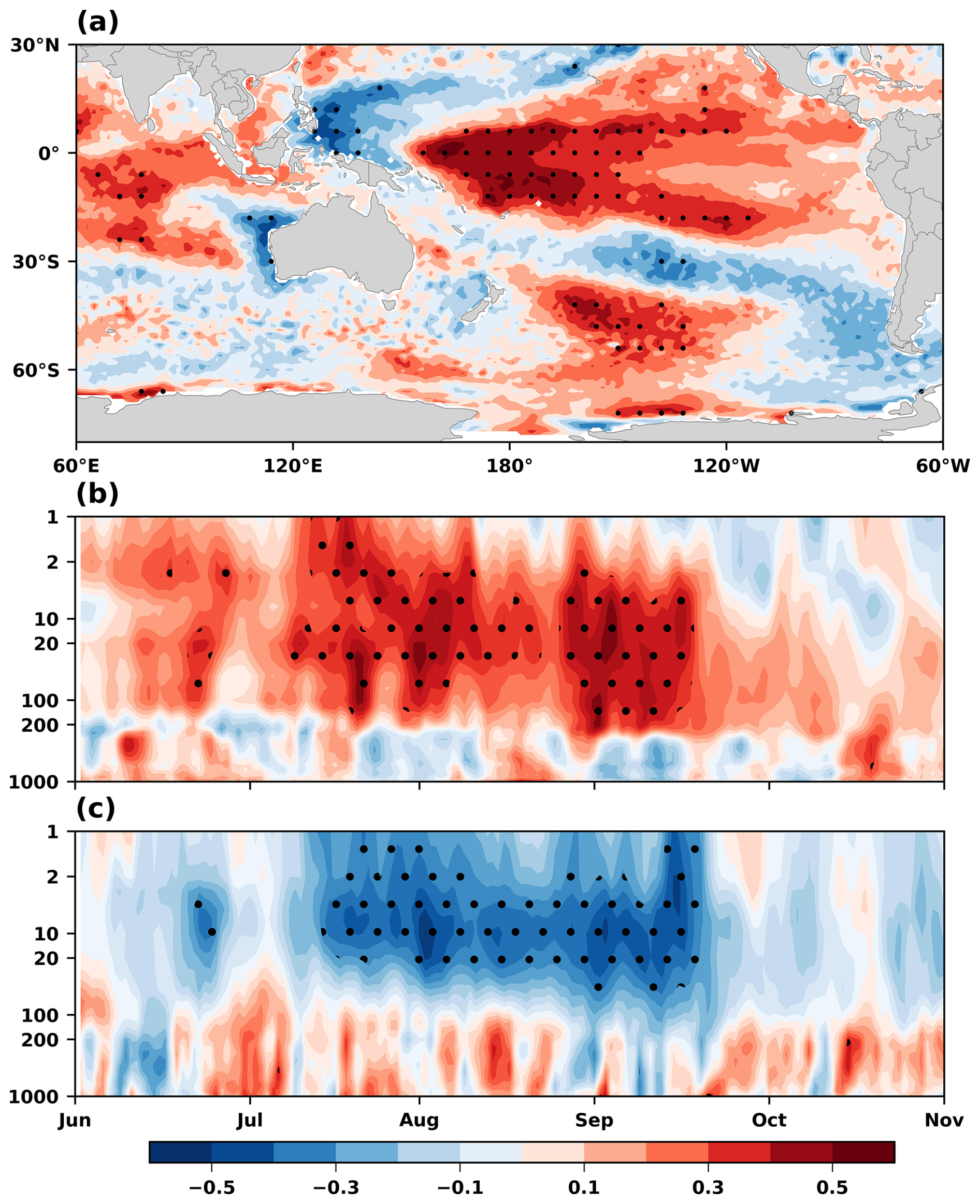
Figure 1 (a) Correlation coefficients between the July–September mean T₁₀₋₃₀ index and January–March mean SST, (b) Correlation coefficients between the December–February mean Niño 4 index and daily Temperature averaged over 60–90° S, and (c) same as (b), but for the zonal-mean zonal wind averaged over 40–50° S. Black dots represent the 95 % confidence level.

The most pronounced impacts of SSTa over the Niño 4 region occur, however, above 100 hPa during the austral winter of the following year. Figure 1b and c present the correlations between the boreal winter Niño 4 index and the Antarctic daily zonal-mean temperature (averaged over 60–90° S) and zonal-mean zonal wind (averaged over 40–50° S) from June–September of the following year. The Niño 4 index exhibits significant positive correlations with stratospheric temperature and negative correlations with zonal wind during July–September (Fig. 1b and c), consistent with the stratospheric warming and weakened SPV.

To further examine the impacts of the Niño 4 SST anomalies on the stratospheric temperatures and the SPV, 17 warm years and 14 cold years defined by ±0.5σ of the Niño 4 index are selected to calculate composite differences in vertical zonal-mean temperature and zonal wind (Fig. 2). The ±0.5σ of threshold value is chosen to capture relatively strong warm and cold events, but the results are not sensitive to the specific threshold value. In June, warming is primarily observed in the upper polar stratosphere and the tropical troposphere, with the strongest signal at 1–5 hPa (Fig. 2a). As the season progresses, the warming intensifies and gradually propagates downward and poleward, with peak anomalies centered around ∼50 ° S in July–August (Fig. 2b and c). This warming reaches its maximum at 10 hPa over 70–90° S in September (Fig. 2d).

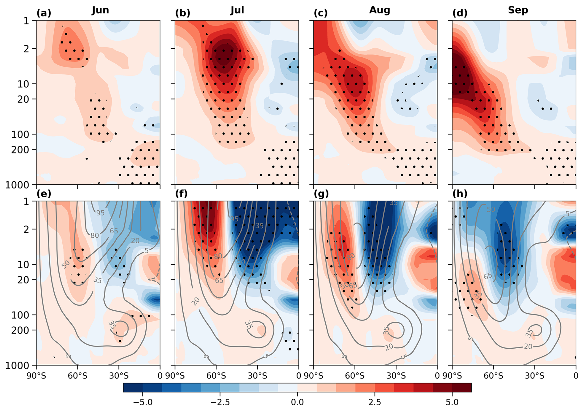
Figure 2 Composite differences between warm and cold Niño 4 years for (a, e) June, (b, f) July, (c, g) August, and (d, h) September. (a–d) Zonal–mean temperature (shaded, unit: K), and (e–h) zonal-mean zonal winds (shaded, unit: m s⁻¹), where the zonal-mean zonal wind climatology is the long-term mean averaged over 1991–2020 (contour, unit: m s⁻¹). Black dots indicate regions statistically significant at the 95 % confidence level.

In general, the stratospheric warming anomalies are accompanied by a significant weakening of the stratospheric westerlies. Under climatological conditions, the polar night jet typically forms and strengthens gradually from June–July, centered near 1 hPa and around 45° S (Fig. 2e, and f). The jet core then migrates poleward and downward in August and weakens in September (Fig. 2g and h). However, during warm Niño 4 years, anomalous easterlies emerge north of 45° S and anomalous westerlies develop south of 45° S as early as June (Fig. 2e), while anomalous easterlies progressively shift poleward from July to September, substantially weakening the climatological westerlies (Fig. 2f–h), indicating a notable poleward contraction and shift of the SPV (Fig. 2f–h). This pattern reflects a delayed yet robust stratospheric response to warm SST anomalies in the tropical central Pacific.

Moreover, the atmospheric responses exhibit the maximum stratospheric warming over the Indian Ocean during June–September, while no significant warming is observed in the South Pacific (Fig. 3a–d). This warming pattern tends to weaken mid-latitude baroclinicity, producing a westerly anomaly at high-latitude and easterly anomalies in the mid-latitude in stratosphere, indicative of a contraction of the jet stream (Fig. 3e and h). Meanwhile, the stratospheric geopotential height show a zonal wave-1 pattern, with a positive center over the Indian Ocean and a negative center over the Pacific and Atlantic, suggesting a role of planetary wave (Fig. 3i–l). The responses intensify from June–September and gradually propagate eastward and poleward (Fig. 3). For example, the maximum westerly anomalies extend into the Pacific polar region by September, while pronounced easterly anomalies develop over the mid-latitude Pacific (Fig. 3h).

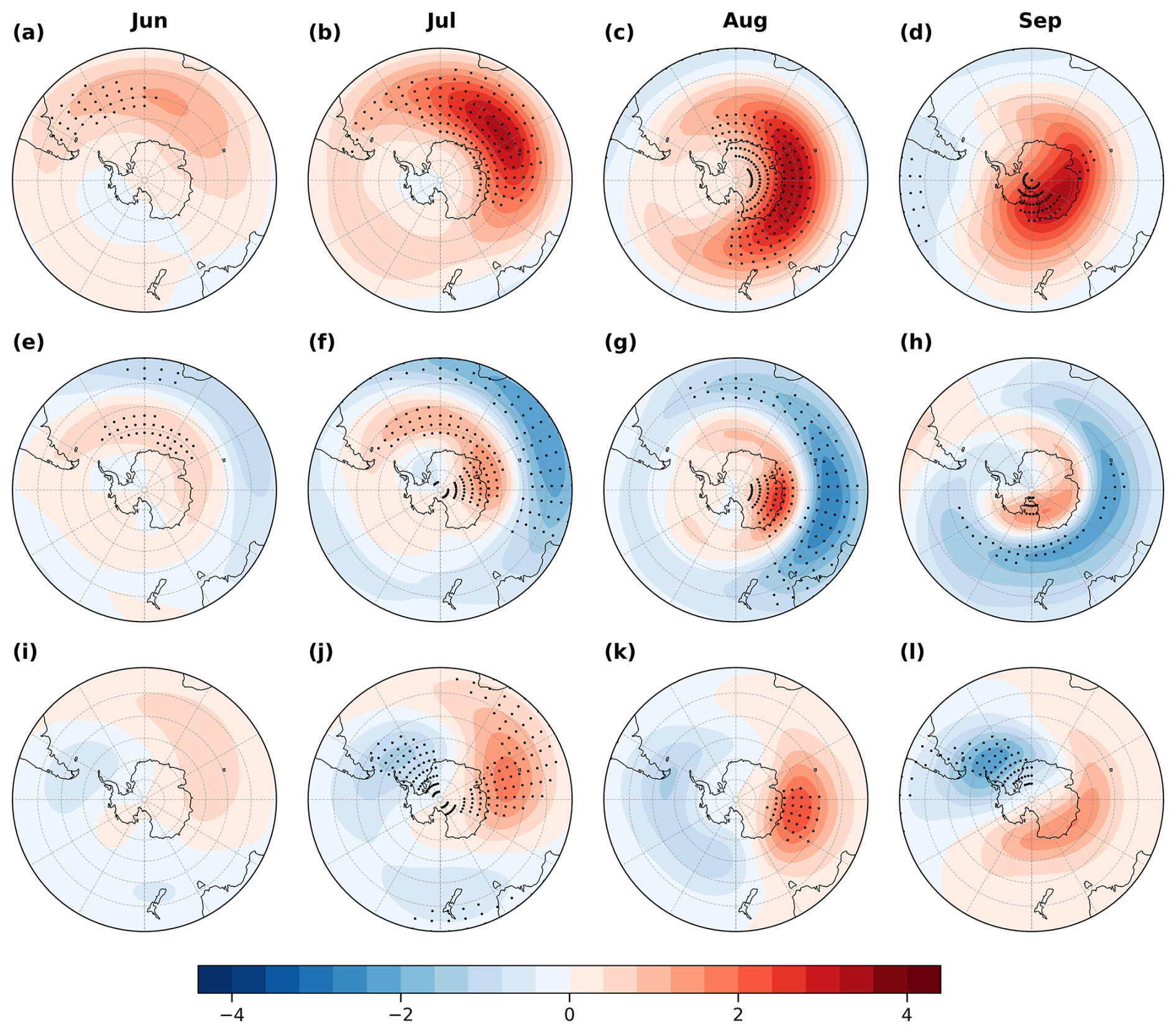
Figure 3 Composite differences between warm and cold Niño 4 years for (a, e, i) June, (b, f, j) July, (c, g, k) August, and (d, h, l) September. (a–d) Temperature averaged over 10–30 hPa (shaded, unit: 2 K), (e–h) zonal wind averaged over 10–30 hPa (shaded, unit: 5 m s⁻¹), and (i–l) geopotential height averaged over 10–30 hPa (shaded, unit: 10 dagpm). Black dots indicate regions statistically significant at the 95 % confidence level.

Following previous studies (Rao et al., 2020; Baldwin et al., 2021; Zi et al., 2025; Lim et al., 2026), the Antarctic stratospheric temperature index (T₁₀₋₃₀) is used to examine the stratospheric response. Although the strongest and most statistically significant correlations between the December–February Niño 4 index and the subsequent July–September Antarctic stratospheric temperature are found over the region spanning approximately 30° E–160° W and 55–75° S (Fig. 3b–d), the T₁₀₋₃₀ index provides a robust and representative diagnostic of Antarctic stratospheric warming, exhibiting a high correlation coefficient (R=0.93) with the temperature index averaged over 30° E–160° W and 55–75° S.

Figure 4a and b present time series of the boreal winter Niño 4 index alongside the July–September mean T₁₀₋₃₀ and U₁₀₋₃₀ indices from 1980–2024. The Niño 4 index exhibits a significant positive correlation with the T₁₀₋₃₀ index (R=0.43, p<0.01) (Fig. 4a) and a significant negative correlation with the U₁₀₋₃₀ index ($R=-\mathrm{0.38}$, p<0.01) (Fig. 4b), both significant at the 99 % confidence level, indicating that a warm (cold) Niño 4 SSTa is typically associated with a warmer (colder) polar stratosphere and contracted (expanded) SPV. Notably, several prominent sudden stratospheric warming (SSW) events (e.g., 1988, 2019, 2024) coincide with positive Niño 4 SSTa (Fig. 4a). The associated stratospheric changes also influence Antarctic ozone concentrations (Wang et al., 2025). For instance, TCO₃ index shows a strong positive correlation with both the T₁₀₋₃₀ index (R=0.56, p<0.01) and the boreal winter Niño 4 index (R=0.36, p<0.01), both statistically significant at the 99 % confidence level (Fig. 4c). This relationship suggests that warm (cold) Niño 4 events enhance (suppress) poleward ozone transport, thereby increasing (decreasing) ozone concentrations over Antarctica.

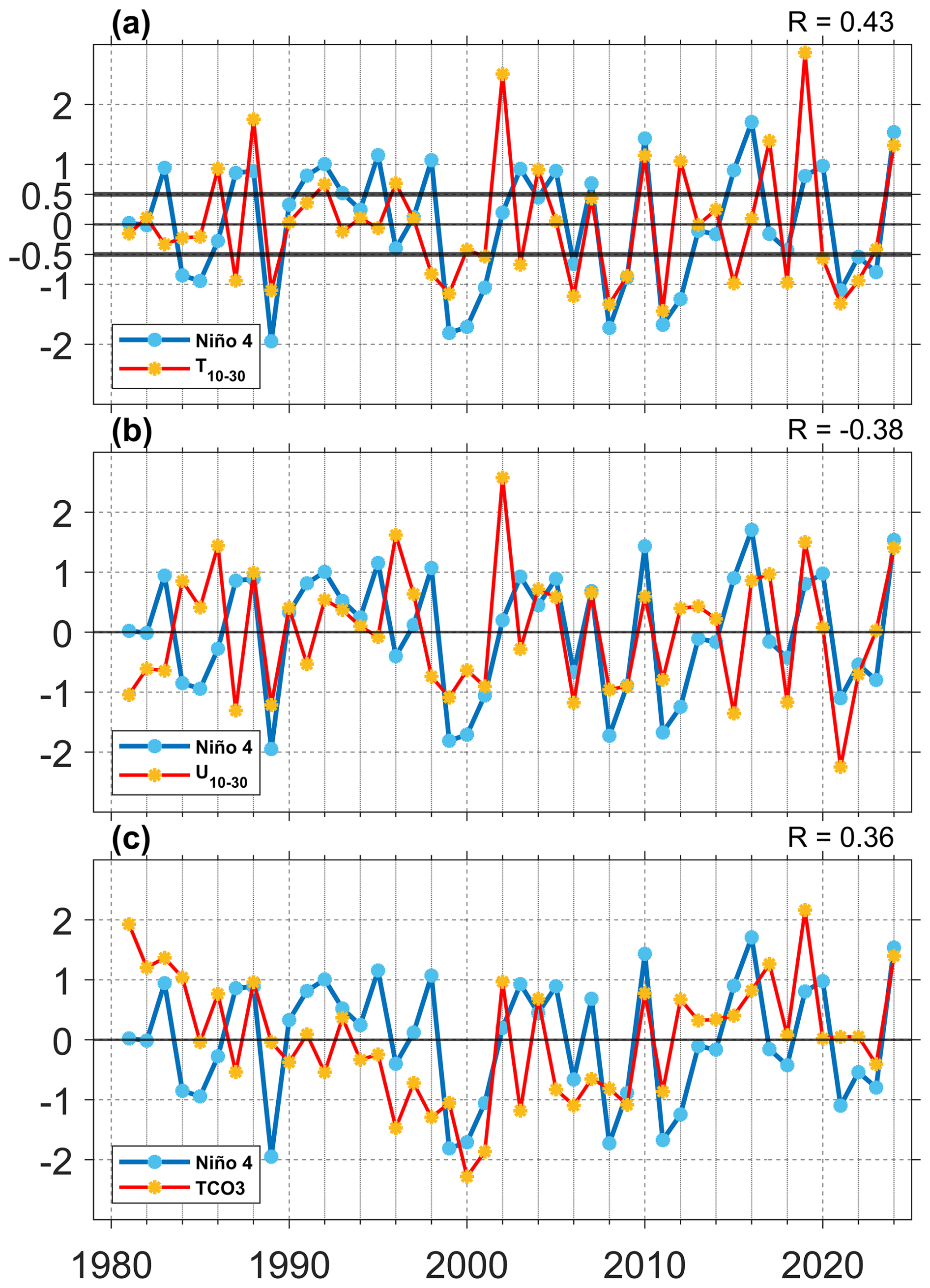
Figure 4 Time series of standardized Niño 4 index (blue line), along with (a) the July–September mean T₁₀₋₃₀ index (red line), (b) the July–September mean U₁₀₋₃₀ index (red line, multiplied by −1), and (c) the July–September mean TCO₃ index (red line) from 1981–2024. R in the upper right corner denotes the correlation coefficient between the Niño 4 index and the T₁₀₋₃₀, $U_{\mathrm{10}-\mathrm{30},}$ and TCO₃ indices, respectively.

4 Effects of anomalous planetary waves

4.1 Stratospheric temperature and zonal wind

Previous studies have suggested that polar stratospheric warming is primarily driven by the upward propagation of planetary waves from the troposphere, which disturb the SPV through wave-mean flow interactions (Baldwin et al., 2021). To evaluate the effect of planetary wave activity on Antarctic stratospheric temperature anomalies during different Niño 4 SST anomalies events, composite differences of key atmospheric variables are calculated between warm and cold Niño 4 years, averaged over consecutive 3-month periods from January to September of the following year.

During the mature phase of El Niño (January–March), positive SST anomalies develop in the tropical central and eastern Pacific (Fig. 5a). As SSTa increases, convection intensifies in the central Pacific (Fig. 5d), accompanied by a negative SLP anomalies and a positive geopotential height anomalies at 250 hPa over the tropical central Pacific, indicating a baroclinic response (Fig. 5g and j). Furthermore, the convection anomaly triggers a southward-propagating teleconnection wave train at 250 hPa, as suggested by the TN01 flux (Vector, Fig. 5j). This wave train, known as the PSA teleconnection (Mo and Higgins, 1998), features a positive geopotential height anomaly over the southeastern Pacific (near 110° W, 60° S) and a negative geopotential height anomaly over the southwestern Pacific (near 150° W, 40° S) (Fig. 5j). The warm Niño 4 SSTa and their associated convection responses over the tropical central Pacific persist into April–June (Fig. 5b, e, h and k). Although the amplitude of the positive and negative height centers over the southeastern and southwestern Pacific weakens, the PSA wave train remains active (Fig. 5k). By July–September (austral winter), however, the warm Niño 4 SSTa and their associated baroclinic responses begin to dissipate (Fig. 5c, i and l). Nevertheless, the negative and positive height centers persists in the southwestern and southeastern Pacific regions, respectively, as indicated by the TN01 flux (Fig. 5l).

Figure 5 Composite differences between warm and cold Niño 4 years. The panels show 3-month means for January–March (left column), April–June (middle column), and July–September (right column). (a–c) Sea surface temperature (SST, shaded, unit: K), (d–f) outgoing longwave radiation (OLR, shaded, unit: $\mathrm{1.5}\times {\mathrm{10}}^{\mathrm{6}}\mathrm{W}{\mathrm{m}}^{-\mathrm{2}}$), (g–i) sea level pressure (SLP, shaded, unit: 300 Pa), (j–l) Geopotential heights (shaded, unit: 5 dagpm) and TN01 flux (vector, unit: 0.1 m² s⁻²) at 250 hPa. Black dots indicate regions statistically significant at the 95 % confidence level.

The geopotential height anomalies extends into the lower stratosphere and remain statistically significant at 100 hPa (Fig. 6a–f). The climatological geopotential height at 100 hPa is characterized by a wave-1 pattern, featuring a positive height center over the South Pacific and a negative height center over the South Atlantic Ocean and South Indian Ocean sectors (contour lines in Fig. 6a–f). During January–February–March (JFM) (austral summer), geopotential height anomalies associated with warm tropical central Pacific SSTa form a wave train, with two positive centers over the southeastern Indian Ocean and southeastern Pacific, and two negative centers over the southwestern Pacific and the southern Atlantic (Fig. 6a). However, the wave-1 pattern at high-latitude is not statistically significant (Fig. 6d). Although the wave-1 component of the geopotential height shows a westward tilt with altiqtude and broadly resembles the climatological structure, this vertical alignment is only statistically significant below 500 hPa (Fig. 6g). As a result, planetary waves are not substantially amplified in the lower stratosphere, primarily due to the prevailing easterly winds in the upper stratosphere over Antarctica during JFM (contours, Fig. 7a), which inhibit upward propagation of planetary waves (Baldwin et al., 2021). This interpretation is further supported by the E–P flux vectors, which show that planetary wave propagation is largely confined below 50 hPa in the mid- and low-latitudes (Fig. 7a).

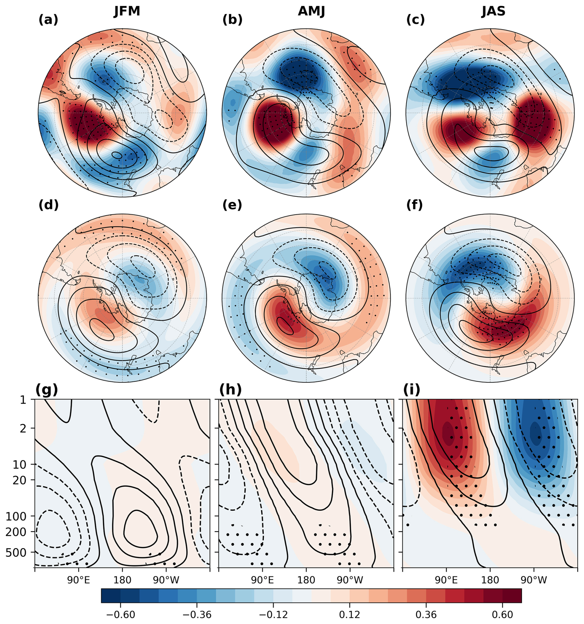
Figure 6 Composite differences between warm and cold Niño 4 years. The panels show 3-month means for January–March (left column), April–June (middle column), and July–September (right column). (a–c) Geopotential heights at 100 hPa (shaded, unit: 5 dagpm), (d–f) wave-1 of geopotential heights at 100 hPa (shaded, unit: 5 dagpm), and (g–i) wave-1 of geopotential heights averaged over 45–75° S at 1000–1 hPa (shaded, unit: 30 dagpm). The climatological geopotential height is the long-term mean averaged over 1991–2020 (contours, unit: dagpm). Black dots indicate regions statistically significant at the 95 % confidence level.

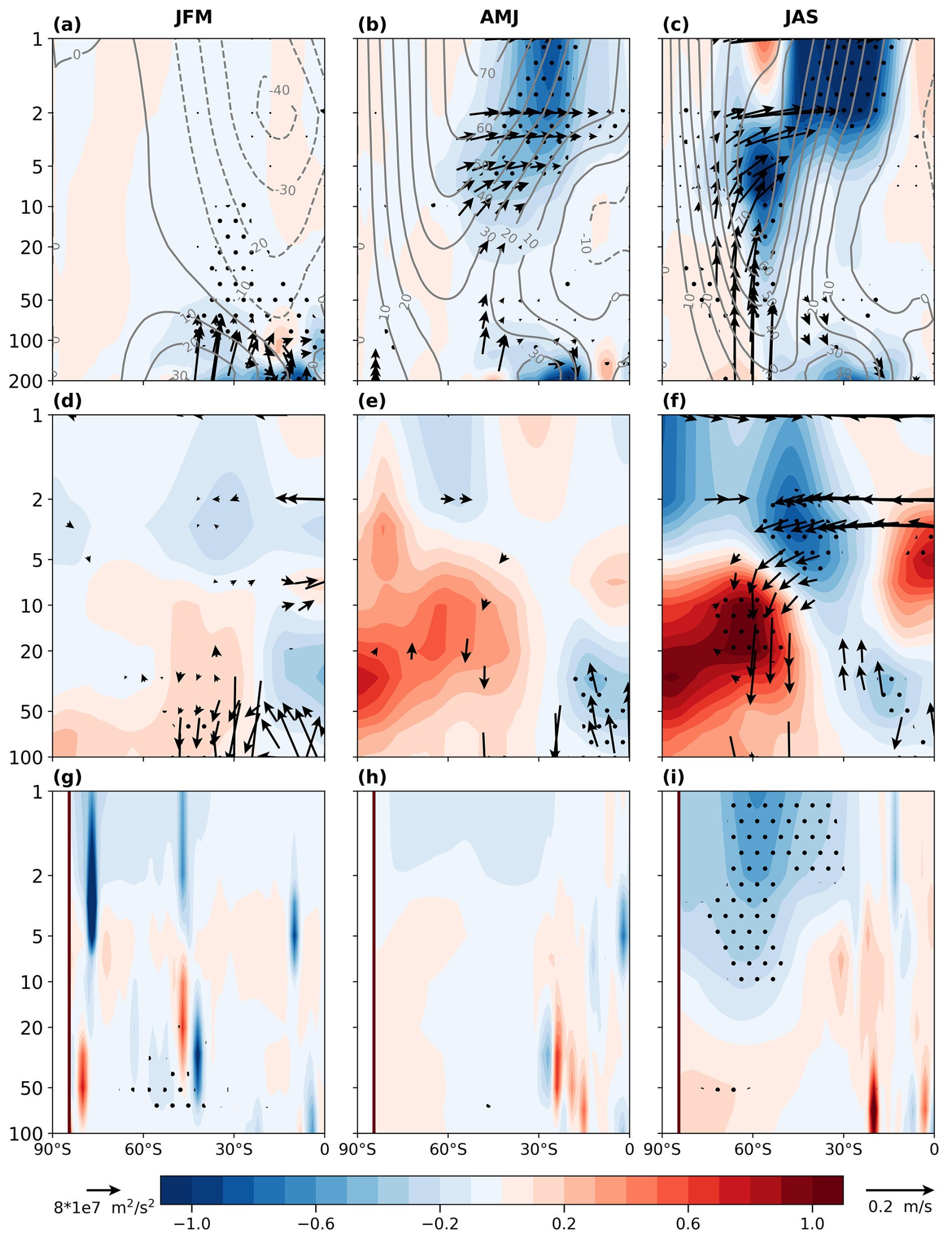
Figure 7 Composite differences between warm and cold Niño 4 years. The panels show 3-month means for January–March (left column), April–June (middle column), and July–September (right column). (a–c) E–P flux (vector: m² s⁻²) and its divergence (shaded, unit: 60 $\mathrm{m}{\mathrm{s}}^{-\mathrm{1}}{\mathrm{d}}^{-\mathrm{1}}$), where the zonal-mean zonal wind climatology is the long-term mean averaged over 1991–2020 (contours, unit: m s⁻¹), (d–f) ozone mass mixing ratio (shaded, unit: $\mathrm{3}\times {\mathrm{10}}^{-\mathrm{6}}$ kg kg⁻¹) and residual mean circulation (vector, unit: m s⁻¹), and (g–i) wave reflective index (shaded, unit: %). Black dots indicate regions statistically significant at the 95 % confidence level.

During April–May–June (AMJ), the positive geopotential height center over the southeastern Pacific and the negative center over the southern Atlantic become more pronounced (Fig. 6b), aligning more closely with the climatological wave-1 pattern (Fig. 6e). This alignment contributes to a westward tilt of the geopotential height field with altitude (Fig. 6h). However, this vertical tilt is only statistically significant below 100 hPa (Fig. 6h). During this period, stratospheric zonal winds gradually transition to a westerly regime, but large portions of the upper polar stratosphere continue to experience weak westerlies or even easterlies (contours, Fig. 7b). As a result, a significant portion of the planetary waves is refracted equatorward, and their ability to disturb the polar stratosphere remains limited (Fig. 7b).

During July–August–September (JAS), the positive height center over the southeastern Pacific weaken, while the positive height center over the southern Indian Ocean strengthens significantly (Fig. 6c). This spatial pattern enhances the climatological wave-1 trough and ridge structure (Fig. 6f) and exhibits a westward tilt of the geopotential height field with altitude, which becomes statistically significant in the stratosphere (Fig. 6i). Although the wave-2 pattern exhibits a strong amplitude, it is nearly orthogonal to the climatological wave-2 phase (figures not shown). Therefore, the wave-2 component is not reinforced, and the process is mainly dominated by the wave-1 pattern. During this period, the polar regions enter the polar night, with minimal solar heating, which increases baroclinicity in the mid- and high-latitude. The stratosphere becomes largely dominated by westerly winds, creating favorable conditions for upward propagation of planetary waves into the polar stratosphere (contour lines, Fig. 7c). In addition, the wave reflection index exhibits a significant negative anomaly south of 30° S in the upper stratosphere (Fig. 7i). This further indicates that planetary waves are strongly refracted toward the mid- and high-latitude stratosphere (Fig. 7c). Based on the E–P flux theorem (Matsuno, 1971), when E–P flux convergence occurs in the mid-latitudes, the jet stream tends to weaken and poleward heat transport increases. During this stage, the strong SPV inhibits the poleward propagation of planetary waves, resulting in relatively weak polar warming and stronger warming in the subpolar and mid-latitude regions. As a result, significant mid- and high-latitude warming and contraction of the SPV are observed (Fig. 3).

This relationship is reversed under cold Niño 4 SSTa conditions. Specifically, when cold SSTa occur in the central tropical Pacific, planetary wave activity and their associated disturbances to the stratosphere are suppressed, leading to polar stratospheric cooling and a extended SPV.

4.2 Mid-latitude sea–air interactions

4.2.1 Ocean responses

The Niño 4 SSTa influence mid-latitude SSTa through atmospheric teleconnections. During JFM, a positive Niño 4 SSTa trigger a PSA teleconnection pattern, resulting in a positive geopotential height anomaly centered near 110° W, 60° S over the southeastern Pacific (Figs. 5j and 7g). The associated poleward surface winds and adiabatic subsidence warm the lower troposphere (Fig. 8a and d). Therefore, the ocean gains heat, as indicated by the negative net heat flux anomaly, leading to a localized SST warming (Fig. 8g). Here net heat flux is defined as the sum of latent and sensible heat fluxes, long-wave radiation and short-wave radiation (Fig. 8m). Simultaneously, there is a modest reduction in SIC in the Amundsen and Ross Seas (Fig. 8j).

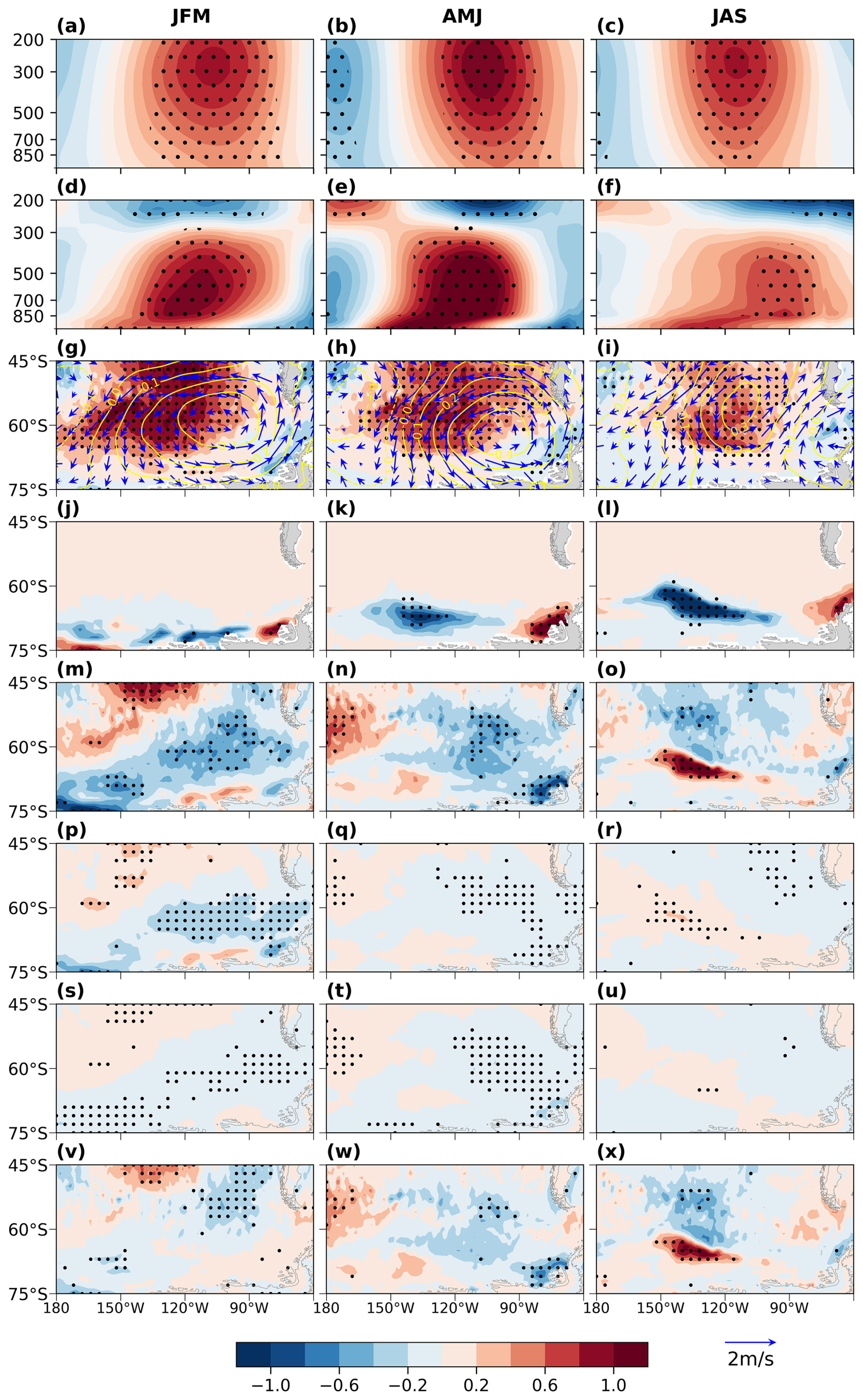
Figure 8 Composite differences between warm and cold Niño 4 years. The panels show 3-month means for January–March (left column), April–June (middle column), and July–September (right column). (a–c) Geopotential heights (shaded, unit: 5 dagpm), averaged over 45–75° S, (d–f) temperatures (shaded, unit: K), averaged over 45–75° S, (g–i) SST (shaded, unit: K), SLP (contours, unit: 1000 Pa), and 10 m winds (vector, unit: 2 m s⁻¹), (j–l) sea ice concentration (SIC, unit: 30 %), (m–o) net upward total heat flux (the sum of turbulence heat flux, upward long-wave heat flux and net downward short-wave radiation, shaded, unit: 3 W m⁻²), (p–r) net downward short-wave radiation (shaded, unit: 3 W m⁻²), (s–u) upward long-wave radiation (shaded, unit: 3 W m⁻²), and (v–x) turbulence heat flux (the sum of latent and sensible heat flux; shaded, unit: 3 W m⁻²). Black dots indicate regions statistically significant at the 95 % confidence level.

A similar pattern persists during AMJ (Fig. 8b and e). The PSA pattern associated with warm Niño 4 SSTa remains evident (Fig. 5k), although the area of negative net heat flux contracts (Fig. 8n), and continues to support SST warming in the southeastern Pacific through ongoing sea–air heat exchange (Fig. 8h). As a result, SIC in the Amundsen and the Ross Seas declines further (Fig. 8k). Additionally, sustained tropospheric warming enhances geopotential height anomalies in both the troposphere and lower stratosphere (Fig. 8b and e).

4.2.2 Ocean feedback to the atmosphere

The tropospheric warming center is located between 500 and 850 hPa during JFM, while the maximum warming shifts below 850 hPa in AMJ and JAS, suggesting an enhanced influence from the ocean surface (Fig. 8d–f). During JAS, Niño 4 SST anomalies weaken (Fig. 5c), indicating a reduced influence of tropical central Pacific SST forcing. Nevertheless, owing to the ocean's large heat capacity, warm SST anomalies in the southeastern Pacific persist (Fig. 8i). As the amplitude of Niño 4 SST anomalies declines, the accumulated heat in the southeastern Pacific is gradually released (Fig. 8o). This heat is transported upward by atmospheric transient eddies and planetary waves generated by enhanced local baroclinicity in the lower troposphere, thereby influencing upper-atmospheric circulation (Nakamura et al., 2008; Sampe et al., 2010). Consequently, a pronounced positive geopotential height anomaly associated with the PSA pattern persists over this region (Fig. 5l).

During JAS, surface net heat flux is largely driven by sea–ice loss in the Amundsen and Ross Seas (Fig. 8l and o). Specifically, the sustained warm SSTa drive substantial sea–ice loss. Comparison between surface heat flux (Fig. 8o) and SIC (Fig. 8l) shows sea–ice loss has a pronounced impacts on surface heat flux. During JAS, solar short-wave radiation reaches its minimum, and its contribution to the net heat flux is relatively small (Fig. 8r). Meanwhile, the contribution from longwave radiation also is relatively weak (Fig. 8u). The primary contributions come from turbulence heat fluxes (Fig. 8x) and temperature advection (Fig. 8i).

During this stage, northerly anomalies dominate the region over 40–60° S, 90–140° W, which transport warm air advection from tropical regions to the mid-latitudes and enhance ocean heat uptake from atmosphere. Although the negative net heat flux anomalies persist north of 60° S, their intensity is relatively weak. In contrast, significant oceanic heat is released to the atmosphere in the regions where sea–ice has retreated (Fig. 8o), warming the lower troposphere (Fig. 8f). In addition, the enhanced heat in the lower troposphere is transported upward, sustaining the positive geopotential height anomaly through the upward displacement of isobaric surfaces (Fig. 8c), consistent with previous studies (Honda et al., 2009; Kim et al., 2014; Yang et al., 2016; Hoshi et al., 2017).

Moreover, near-surface heating associated with sea–ice loss acts as an effective source of planetary wave under wintertime background conditions, contributing to the amplification of zonal wave patterns and enhanced planetary wave propagation (Kim et al., 2014; Nakamura et al., 2015). Notably, while net heat flux is dominated by ocean heat uptake during JFM and AMJ, the influence of sea–ice loss becomes predominant in JAS, resulting in net heat release from the ocean to the atmosphere (Fig. 8m–o). This positive feedback reinforces the Southern Hemisphere zonal-wave pattern and amplifies the planetary wave anomalies (Zi et al., 2025). Recent modeling studies also suggest that sea–ice loss in the Amundsen Sea and the broader Antarctic region can have pronounced impacts on the SPV (Song et al., 2025). Therefore, the sea–ice loss tends to sustain the influence of the Niño 4 SSTa on stratospheric temperatures during JAS by enhancing surface heat fluxes (Fig. 8).

4.3 Ozone transport

The enhanced planetary wave associated with the warm Niño 4 SSTa not only warms the polar stratosphere but also significantly alters the B–D circulation and polar ozone transport (Wang et al., 2025). Figures 7d–f present the composite differences in the zonal-mean residual circulation and ozone mass mixing ratio between warm and cold Niño 4 years, averaged over consecutive 3-month periods from January–September of the following year.

During JFM, convective anomalies in the tropical Pacific Ocean drive changes in the residual circulation (Fig. 5d), resulting in decreased ozone mass mixing ratio in the tropical lower stratosphere and increased values in the mid-latitude lower stratosphere (Fig. 7d). However, upward–propagating planetary waves are largely confined below 50 hPa in the mid- and low-latitude (Fig. 7a), strengthening the residual circulation primarily north of 60° S. As a result, ozone transport to higher altitudes and into the polar region remains limited (Fig. 7d). During AMJ, although convective anomalies in the tropical Pacific Ocean persist and planetary wave increases in the upper stratosphere (Fig. 7b), many of the waves are refracted equatorward, resulting in only modest enhancement of polar ozone transport (Fig. 7e). During JAS, however, upward–propagating planetary waves are strongly refracted toward mid- and high-latitude, enhancing the residual circulation and promoting poleward ozone transport (Fig. 7f). The increased poleward ozone transport enhances solar radiation absorption, playing an important role in the polar stratospheric warming through dynamical–chemical coupling (Solomon et al., 2016). In addition, adiabatic warming associated with descending motion in the residual circulation further contributes to the stratospheric warming over the polar region.

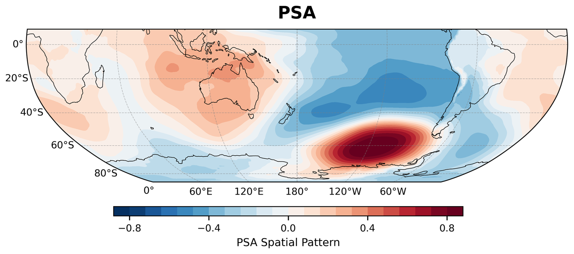
Figure 9 PSA teleconnection pattern represented by the second EOF mode of monthly SLP.

5 Multivariate regression model

The preceding analyses reveal that boreal winter Niño 4 SSTa exert a significant lagged influence on the Antarctic stratospheric circulation during the subsequent austral winter. This finding has important implications for the seasonal prediction of stratospheric variability. However, although the boreal winter Niño 4 index is significantly correlated with the July–September mean T₁₀₋₃₀ index, it accounts for only 18.5 % of the variance in stratospheric temperature (R²=0.185). To better interpret variability in the Antarctic stratosphere, additional factors need to be considered.

Previous studies have found that the PSA teleconnection associated with the Niño 4 SSTa is a key mechanism influencing the Antarctic stratosphere. The PSA pattern is represented by the second EOF mode of monthly SLP anomalies (Fig. 9). The corresponding PSA index is defined as the time series of this EOF mode. During boreal winter, the PSA index is significantly and simultaneously correlated with the Niño 4 index (R=0.40, p<0.01), suggesting that the Niño 4 SSTa modulate the PSA pattern. However, the correlation between the June PSA index and the boreal winter Niño 4 index is relatively weak (R=0.28, p<0.05). In addition, the June PSA index is significantly correlated with May–June mean Antarctic sea–ice (R=0.49, p<0.01), suggesting that the June PSA pattern may be maintained by sea–ice anomalies and other factors. Furthermore, correlations between the PSA index from December through the following September and the July–September mean T₁₀₋₃₀ index shows that the June PSA index exhibits the strongest relationship with Antarctic stratospheric temperature during JAS (R=0.47, p<0.01, Table 3).

Table 3 Correlation coefficients between the July–September mean T₁₀₋₃₀ index and the SIC index (SIC_AR) averaged over the Amundsen and Ross Seas (180–90° W), the SST index over the South Pacific (SST_SP) and the PSA index.

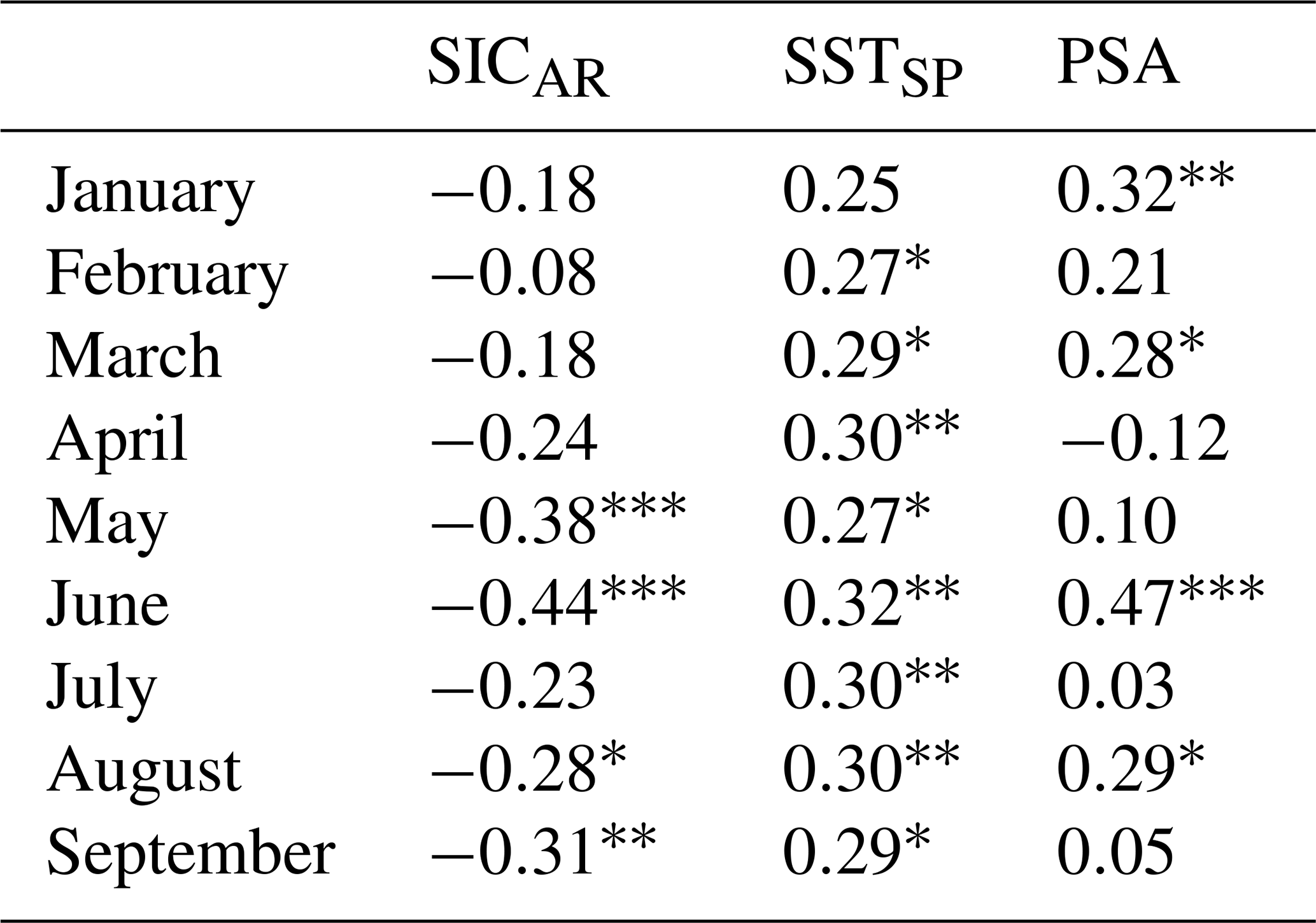
Note: asterisks denote statistical significance: ${}^{***}$ represent 99 % confidence level, ${}^{**}$ for 95 %, and ^* for 90 %.

As a result, a multivariate linear regression (MLR) model is used to quantitatively assess the linear relationship between the stratospheric temperature index (T₁₀₋₃₀) and potential factors including the Niño 4 and PSA indices. We have

$$\begin{array}{}\text{(9)}& T_{\mathrm{10}-\mathrm{30}}={\mathit{\beta }}_{\mathrm{0}}+{\mathit{\beta }}_{\mathrm{1}}\text{Niño4}+{\mathit{\beta }}_{\mathrm{2}}\text{PSA}+\mathit{\epsilon },\end{array}$$

where β₀ is the intercept, β₁, β₂ are the regression coefficients associated with each factor, and ε denotes the residual error term. Prior to the regression analysis based on Eq. (9), all input time series are standardized. The regression analysis is performed using MATLAB's fitlm function, which yields estimates of regression coefficients, standard errors, t statistics, and p values, along with overall model diagnostics, such as the coefficient of determination (R²) and the F-statistic. To evaluate the significance of individual factors, three confidence levels are adopted: 90 %, 95 %, and 99 %, corresponding to p-value thresholds of 0.1, 0.05, and 0.01, respectively. Factors with p values below these thresholds are considered statistically significant. The overall performance and goodness-of-fit of the model are assessed using the R² metric.

To better predict the July–September mean T₁₀₋₃₀ index, the boreal winter Niño 4 (Niño4_DJF) index and the June PSA (PSA_Jun) index are used as predictors in Eq. (9). The resulting regression relationship is

$$\begin{array}{}\text{(10)}& T_{\mathrm{10}-\mathrm{30}}=\mathrm{0.324}\text{Niño4\_DJF}+\mathrm{0.384}\text{PSA\_Jun}+\mathit{\epsilon },\end{array}$$

where β₀=0. This linear regression model yields a coefficient of determination (R²) of 0.321, indicating that the predictors collectively explain approximately 32 % of the variance in the July–September mean T₁₀₋₃₀ index. The model's F-statistic is 9.71 with a corresponding p value of 0.00035, which is significant at the 99 % confidence level. Among the predictors, the Niño4_DJF and PSA_Jun exhibit statistically significant regression coefficients (p=0.0201 and p=0.0065, respectively), confirming their dominant roles in modulating stratospheric temperature variability.

To assess model performance, the regression–based fitted index (referred to as NP_fit) is compared with the observed July–September mean T₁₀₋₃₀, U₁₀₋₃₀, and TCO₃ (Fig. 10). The NP_fit index shows significant correlation with the observed values for T₁₀₋₃₀ (R=0.57, p<0.01), U₁₀₋₃₀ ($R=-\mathrm{0.55}$, p<0.01), and TCO₃ (R=0.32, p<0.05). The correlations are stronger than those obtained using the Niño 4 index alone for T₁₀₋₃₀ and U₁₀₋₃₀ (R=0.43 and −0.38, respectively), except for TCO₃ (R=0.36), which the improvement is modest (Fig. 4). While the boreal winter Niño 4 index plays a key role in Antarctic stratospheric temperature variability, incorporating the June PSA index further improves the representation of this variability. This underscores the importance of both tropical forcing and extratropical feedback processes in modulating polar stratospheric circulation.

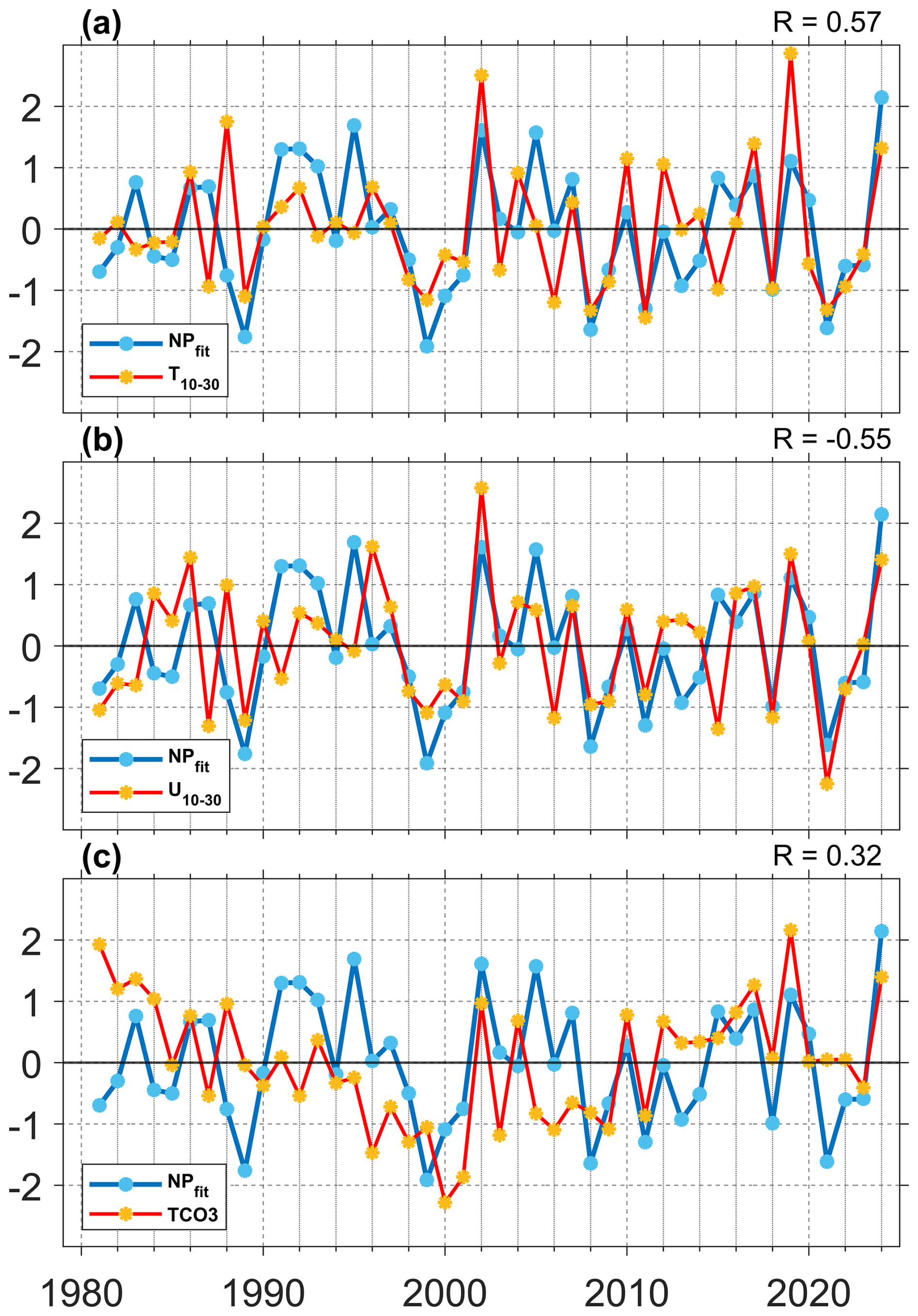
Figure 10 Time series of the standardized NP_fit index (blue line), along with (a) the July–September mean T₁₀₋₃₀ index (red line), (b) the July–September mean U₁₀₋₃₀ index (red line, multiplied by −1), and (c) the July–September mean TCO₃ index (red line) from 1981–2024. R in the upper right corner is the correlation coefficient between NP_fit index and T₁₀₋₃₀, $U_{\mathrm{10}-\mathrm{30},}$ and TCO₃ indices, respectively.

6 CMIP6 results

To further assess the cross-seasonal effects of tropical central Pacific SSTa on Antarctic stratospheric temperature, we analyze 24 CMIP6 historical fully coupled model simulations covering the period 1951–2014. For each model, the Niño 4 index is first calculated following the same procedure used in the observational analysis. Warm and cold Niño 4 years are identified using a threshold of ±0.5σ. Composite differences between warm and cold years are then constructed for DJF mean SST (Fig. 11), JAS mean temperatures at 10 hPa (Fig. 12), JAS mean SST (Fig. 13), and JAS mean Antarctic SIC (Fig. 14).

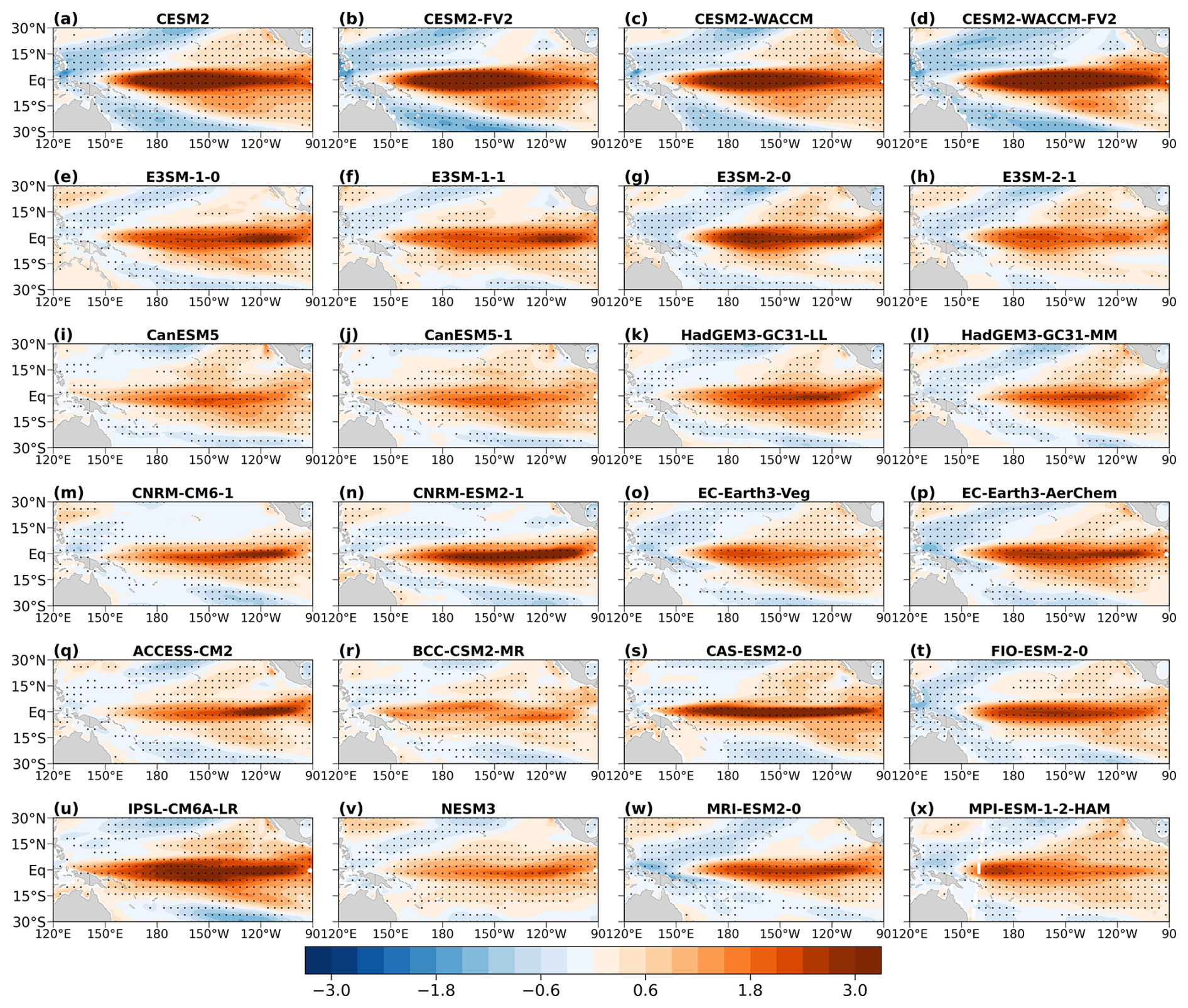
Figure 11 Composite differences in December–February mean SST (shaded, unit: K) between warm and cold Niño 4 years in 24 CMIP6 experiments. Black dots indicate regions statistically significant at the 95 % confidence level.

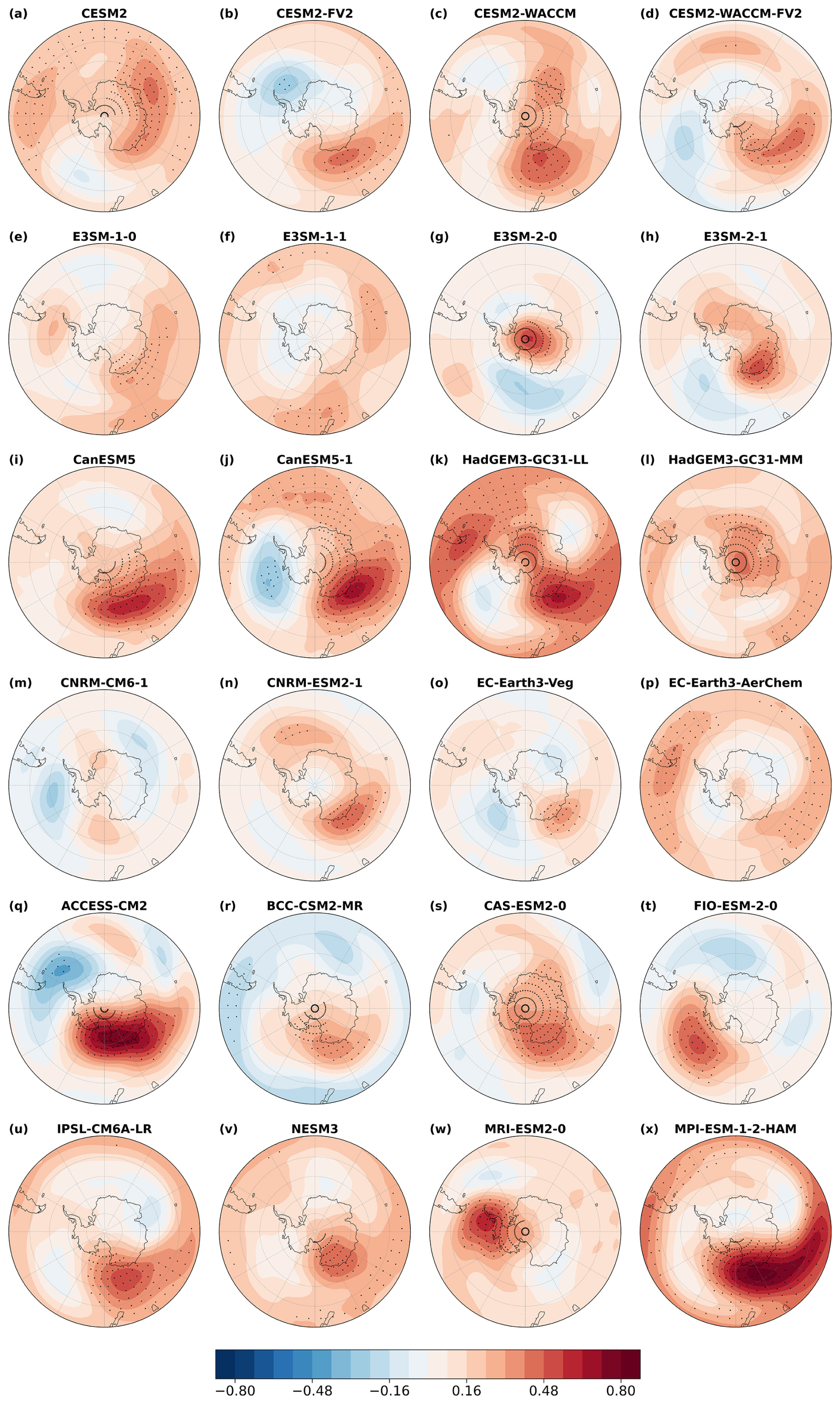
Figure 12 Composite differences in July–September mean temperature (shaded, unit: K) at 10 hPa between warm and cold Niño 4 years in 24 CMIP6 experiments. Black dots indicate regions statistically significant at the 95 % confidence level.

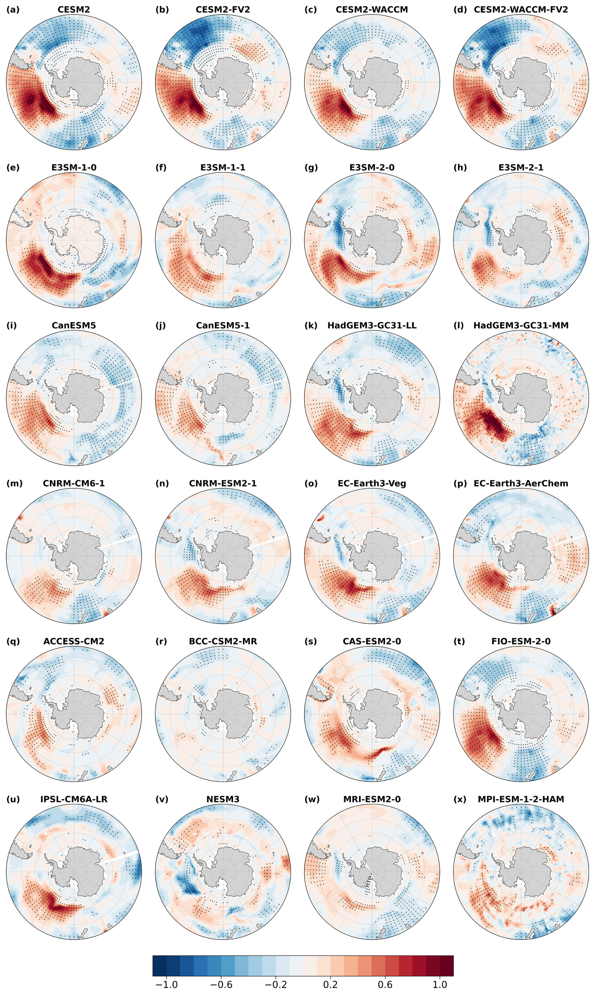
Figure 13 Composite differences in July–September mean SST (shaded, unit: K) between warm and cold Niño 4 years in 24 CMIP6 experiments. Black dots indicate regions statistically significant at the 95 % confidence level.

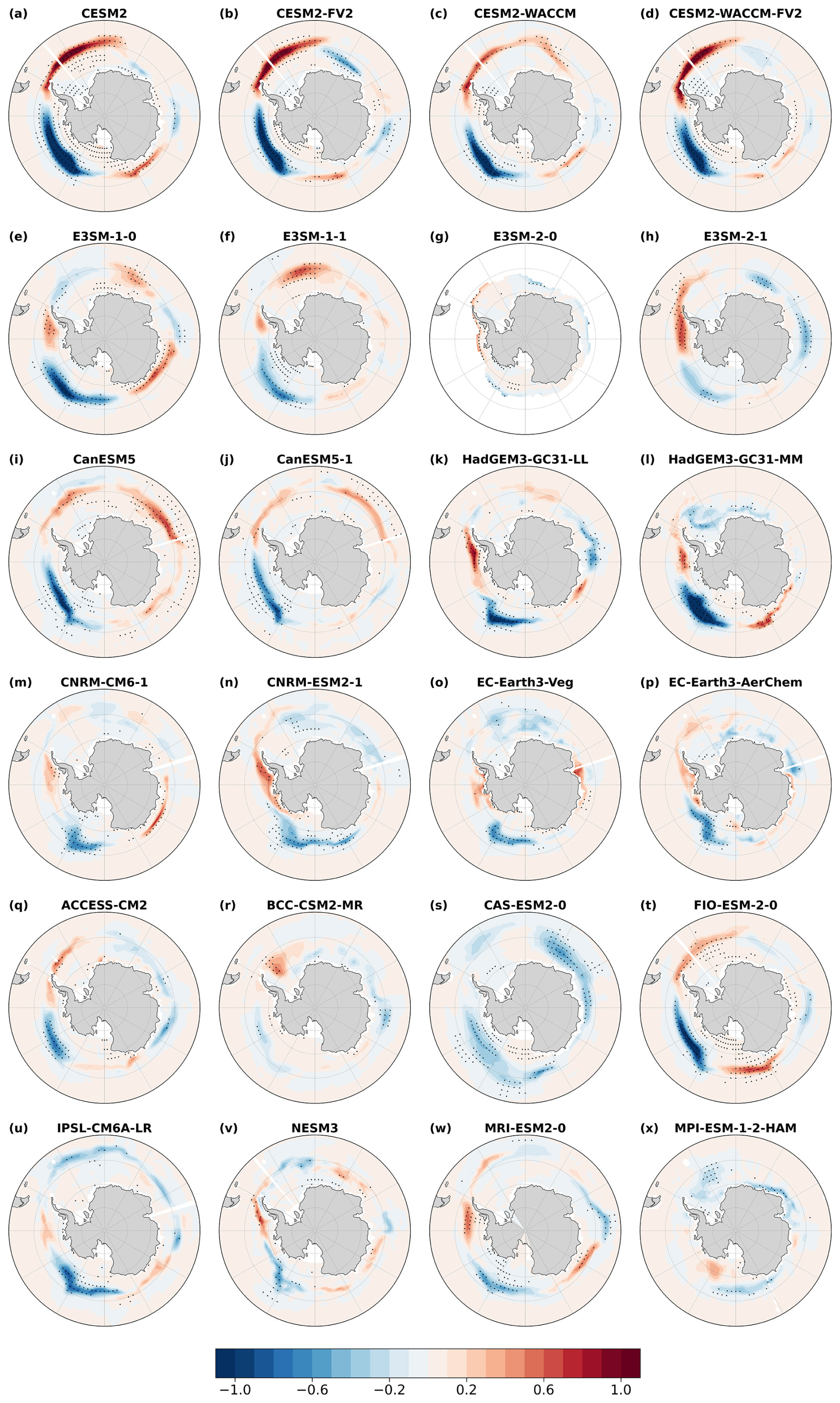
Figure 14 Composite differences in July–September mean SIC (shaded, unit: 30 %) between warm and cold Niño 4 years in 24 CMIP6 experiments. Black dots indicate regions statistically significant at the 95 % confidence level.

In the DJF mean SST, significant warm SSTa consistently emerge over the tropical central Pacific in all models (Fig. 11). Consistent with the observational results, warm SSTa over the tropical central Pacific during the boreal winter are significantly associated with Antarctic stratospheric warming in the subsequent austral winter (Fig. 12). Although the magnitude of the JAS mean Antarctic stratospheric warming at 10 hPa varies among models, for example, relatively stronger warming is simulated in CanESM5, CanESM5-1, HadGEM3-GC31-LL, ACCESS-CM2, and MPI-ESM-1-2-HAM (Fig. 12i, j, k, q and x), whereas weaker warming is evident in models such as E3SM-1-1, CNRM-CM6-1, and EC-Earth3-Veg (Fig. 12f, m and o). Nevertheless, most models exhibit statistically significant warm anomalies. Moreover, consistent with the observations, the warming signal in most models is predominantly located in the Eastern Hemisphere (Figs. 12 and 3b–d), with only a few models (e.g., CNRM-CM6-1, FIO-ESM-2-0, and MRI-ESM2-0) showing warming maxima in the Western Hemisphere (Fig. 12m, t and w).

In addition, the July–September mean SST exhibits a statistically significant positive anomalies over the southeastern Pacific (Fig. 13). Similarly, Antarctic SIC shows pronounced negative anomalies over the Amundsen Sea and Ross Sea sectors (Fig. 14), indicating reduced sea–ice concentration. Although a small number of models (e.g., E3SM-2-0, BCC-CSM2-MR, and MPI-ESM-1-2-HAM) display relatively weaker sea–ice loss (Fig. 14g, r and x), the overall response is consistent across models.

Therefore, these results are consistent with observations and support the existence of a cross-seasonal linkage between tropical central Pacific SSTa and Antarctic stratospheric polar temperature anomalies.

7 Conclusions and discussions

The cross-seasonal influence of tropical central Pacific sea surface temperature (SST) on Antarctic stratospheric circulation has been investigated in this study using 45 years (1980–2024) ERA5 reanalysis. Our analysis reveals that warm (cold) SSTa in the Niño 4 region (Central Pacific) during boreal winter are followed by significantly warming (cooling) of the Antarctic stratosphere in the subsequent austral winter (July–September), accompanied by a contracted (expanded) stratospheric polar vortex (SPV). Among the ENSO indices examined (Niño 3, Niño 3.4, Niño 4), the boreal winter Niño 4 index exhibits the strongest and most robust correlation with the July–September polar stratospheric temperature (T₁₀₋₃₀) index, reaching R≈0.43 (p<0.01). In contrast, correlations with the Niño 3.4 and Niño 3 indices (Eastern Pacific) are substantially weaker, suggesting that the Niño 4 SSTa are the primary drivers of the observed Antarctic stratospheric responses. In addition to the observational analyses, fully coupled simulations from 24 CMIP6 models also reproduce the cross-seasonal linkage between tropical central Pacific SSTa and Antarctic stratospheric temperature variability, providing further evidence for the robustness of the identified teleconnection.

In this study, both the tropical central Pacific SST and the Antarctic stratospheric indices exhibit notable variability on decadal timescales (Fig. 4a). To account for the influence of the decadal variability, a 10-year low-pass filter is applied to the Niño 4 and T₁₀₋₃₀ indices to extract their decadal components (Fig. 15a). The interannual components are then obtained by subtracting the decadal signals from the original time series (Fig. 15b). The decadal components exhibit a much stronger correlation of 0.82 (p<0.01), indicating that a pronounced decadal-scale relationship exists between the two indices. Importantly, the interannual components also remain significantly correlated, with a correlation coefficient of 0.41 (p<0.01). Although this correlation is slightly weaker than that of the original series (Fig. 4a), it remains statistically robust, demonstrating the tropical central Pacific SSTa exert a significant influence on Antarctic stratospheric temperature variability at interannual timescales.

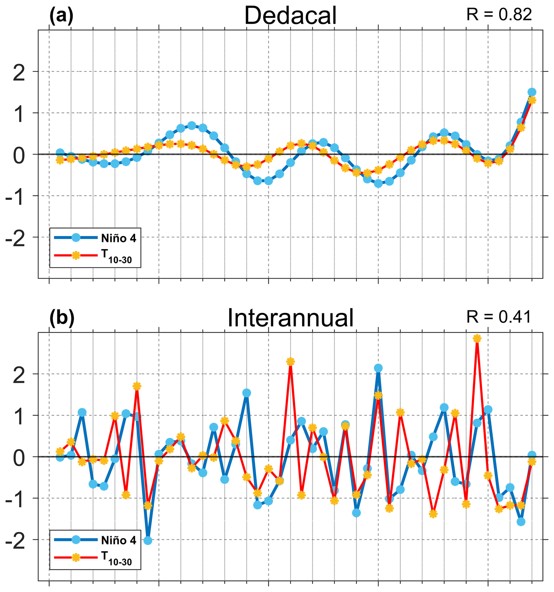
Figure 15 Time series of standardized Niño 4 index (blue line) and the July–September mean T₁₀₋₃₀ index (red line). Panels (a) and (b) show the decadal and interannual components, respectively. The value R in the upper right corner denotes the correlation coefficient between the Niño 4 and T₁₀₋₃₀ indices.

The underlying dynamics involve the Pacific–South America (PSA) teleconnection pattern triggered by the Niño 4 SSTa and mediated through wave-mean flow interactions. During boreal winter, warm SSTa in the Niño 4 region enhance convection near the dateline, exciting a Rossby wave train that propagates poleward and eastward across the Southern Hemisphere. This wave activity generates a positive geopotential height anomaly over the southeastern South Pacific and a negative anomaly over the South Atlantic, thereby reinforcing the climatological wave-1 ridge and trough structure. As the seasonal transition toward austral summer and winter progresses, the Antarctic stratospheric circulation shifts toward a predominantly westerly regime, creating favorable conditions for the upward propagation of planetary waves into the polar stratosphere. Subsequent convergence of Eliassen–Palm (E–P) flux, followed by wave breaking, induces stratospheric warming and a deceleration of the SPV.

It is also found that warm SSTa in the South Pacific and sea–ice loss over the Amundsen and Ross Seas can reinforce the mid- and high-latitude zonal wave train through sea–air interactions. Specially, the PSA teleconnection associated with Niño 4 warming drives ocean heat uptake and rising SSTa in the southeast Pacific from January–March through April–June. With progression of seasons, this remote tropical forcing weakens during June–September, and a local sea–air feedback becomes dominant. Persistent warm waters accelerate sea–ice melt, and the subsequent oceanic heat release sustains the positive geopotential height anomalies, thereby strengthening the planetary wave response.

Furthermore, stronger planetary wave anomalies induced by warm Niño 4 SSTa play a crucial role in modulating Antarctic ozone transport. These waves enhance the Brewer–Dobson circulation, facilitating the ozone transport from the tropics to the polar stratosphere and leading to elevated ozone concentrations over Antarctica. The increased ozone concentrations enhance ultraviolet absorption, further amplifying stratospheric warming. Simultaneously, the warmer stratosphere inhibits the formation of polar stratospheric clouds (PSCs), thereby suppressing the heterogeneous chemical reactions responsible for ozone depletion and mitigating Antarctic ozone loss (Solomon et al., 2016).

To synthesize these processes, Fig. 16 provides a schematic of the proposed physical mechanism. It illustrates how boreal winter Niño 4 SST anomalies trigger a sequence of dynamical and thermodynamical responses, including enhanced tropical convection, the PSA teleconnection, planetary wave propagation, mid-latitude air–sea feedbacks, strengthened Brewer–Dobson circulation, and ozone transport, which collectively lead to Antarctic stratospheric warming during the subsequent austral winter.

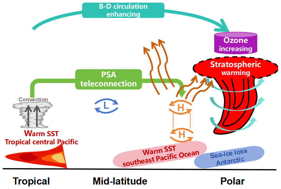
Figure 16 Schematic diagram illustrating the proposed physical mechanism linking boreal winter Niño 4 SST anomalies to Antarctic stratospheric warming in the subsequent austral winter.

A multivariate regression statistical model was used in this study to quantify the linear relationship between stratospheric temperature variations and Niño 4 SSTa. The boreal winter Niño 4 index alone accounts for approximately 18 % of the variance in July–September polar stratospheric temperatures. However, including the June PSA index nearly doubles the explained variance to 32 %. This highlights the combined role of tropical forcing and mid-latitude atmospheric responses in shaoing stratospheric temperature variability. Nonetheless, a substantial portion of stratospheric variability remains unexplained. This reflects the internal influence of atmospheric internal dynamics, as well as contributions from other drivers such as the Quasi-Biennial Oscillation (QBO), solar activity, and mid-latitude tropospheric wave sources. Additional factors may be identified through a range of approaches, including numerical modeling, machine learning, and causal inference.