
the Creative Commons Attribution 4.0 License.
the Creative Commons Attribution 4.0 License.
 | 19 Nov 2026
Insights into the chemical and physical drivers of surface ozone in the Trans-Himalaya

Mehul R. Pandya
Tabish Ansari
Sonam Angmo
Subrat Sharma
Bipasha Paul Shukla
Aditya Vaishya
Lokesh Kumar Sahu
Tim Butler
Narendra Ojha
The Trans-Himalaya, located between the Great Himalaya and the Tibetan Plateau, is ecologically fragile and one of the most climate-sensitive regions. However, lack of systematic in situ measurements have hindered the evaluation of chemistry–climate models and constrained our understanding of the global-to-regional influences over this region. To address this, we present a comprehensive analysis by combining first yearlong (October 2024–September 2025) surface ozone (O3) measurements at Leh (3.4 km above mean sea level) with satellite data and numerical simulations (global model: CAM4-Chem, regional model: WRF-Chem). Our measurements revealed a noontime O3 build-up (∼ 3–7 ppbv), a feature typically absent over high altitude mountains. WRF-Chem suggests that this feature is driven by photochemical production (NOx-VOC transition regime for higher O3) and entrainment. Despite partial compensation of nighttime loss by noontime build-up, the region acts as a net chemical sink. Seasonal cycle peaks in June (∼ 65 ± 6 ppbv; touching air quality threshold), unlike typical premonsoon peaks over Gangetic and Himalayan regions. CAM4-Chem simulation with CAMS-derived stratospheric contribution, captured the O3 seasonality, but overestimated the wintertime levels by 10–15 ppbv. Tagged O3-tracer analysis shows significant contributions of anthropogenic NOx emissions from South Asia (15 %–18 %) and other regions (32 %–37 %) to O3 levels. Additionally, stratospheric inputs and biogenic emissions shape the seasonal cycle. This study provides insight into the chemistry and dynamics governing O3 over the Trans-Himalaya across different time scales. These findings are invaluable for designing future field observations, model improvements, and policy planning for this region.
- Article
(12422 KB) - Full-text XML
-
Supplement
(3379 KB) - BibTeX
- EndNote


Tropospheric ozone (O3) plays a tripartite role: a primary controller of the atmosphere's oxidative capacity, a significant short-lived climate forcer, and a secondary air pollutant (Seinfeld and Pandis, 2016). High levels of ground level O3 adversely impact human health, vegetation, crop yield and ecosystem (Chuwah et al., 2015; US EPA, 2013). Tropospheric O3 also acts as a greenhouse gas, produced photochemically by methane (CH4), carbon monoxide (CO), and non-methane hydrocarbons (NMHCs) in the presence of nitrogen oxides (NOx). Thus, O3 is considered an important link between air quality and climate. O3 has a longer lifetime (6–27 d) in the free troposphere compared to the boundary layer (few hours to ∼ 1 week), due to weaker loss processes associated with lower water vapour and negligible deposition (Prather and Zhu, 2024). Therefore, free-tropospheric O3 levels can sustain more than those within the urban or rural local boundary layers, and hence such observations would be better representative of regional conditions. In addition, free tropospheric O3 variations can provide insights into vertical transport including stratospheric intrusions as well as in situ or en-route O3 formation through convectively transported precursors (Ansari et al., 2025; Nalam et al., 2025; Ojha et al., 2012; Sahu et al., 2009; Sinha et al., 2016). O3 mixing ratios generally increase with altitude owing to more intense solar radiation and low concentrations of the titrating gases, for example, NO (Chevalier et al., 2007). The intrusions of O3-rich stratospheric air also enhance O3 levels more at higher altitudes compared to low-altitude plain regions (Cristofanelli et al., 2010). Therefore, studies on O3 variations at high-altitude remote stations are critical to obtain comprehensive insights into the roles of regional emissions, photochemistry, long-range transport, and stratospheric intrusions (Kumar et al., 2010; Sarangi et al., 2014).
Ladakh is a Union Territory (a region directly governed by the central government) and the northern-most part of India, situated in the Trans-Himalayan region between the Karakoram and Great Himalayan ranges. It is one of the coldest, driest and most sparsely populated regions in South Asia and is suggested to be one of the most climate-sensitive, highly vulnerable, and ecologically fragile regions of the world (Goodrich et al., 2019; Wester et al., 2019). Ladakh lies in one of the three sub-divisions of Hindu Kush Himalaya (HKH), i.e., north-western Himalaya and Karakoram range (32–39° N; 71–79° E). The International Centre for Integrated Mountain Development (ICIMOD) have reported that HKH is warming faster than the average rate of global warming with adverse impacts on the cryosphere, hydrology, ecology, vegetation, wildlife, and human society (Nair et al., 2024; Wester et al., 2019). Annual mean temperature has risen by more than 2 °C in Leh region over the period of 13 years (1995–2009; Chevuturi et al., 2018). This region is already experiencing substantial consequences of the climate change, e.g., increased glacier retreating, water scarcity, heatwaves, landslides, flash floods, debris flows, and soil erosion, etc (Bhattacharjee and Dutta, 2023; Dubey et al., 2025; Khanday et al., 2024; Pandit, 2013; Ziegler et al., 2016). Being a high-altitude region, remote from major anthropogenic emissions, Ladakh experiences a cleaner background atmospheric conditions, as compared to the densely populated and global hotspot of emissions – the Indo–Gangetic Plain (IGP) in its immediate south. Due to spatial proximity plus strong atmospheric dynamics, the transport of trace gases and aerosols from IGP can potentially influence the Trans-Himalaya also, as observed for the Himalayan region (Das et al., 2022; Hassan et al., 2023; Ojha et al., 2012; Sarangi et al., 2014). Signatures of aged background aerosols as well as new-particle formation from gaseous precursors suggest a unique chemical environment over Trans-Himalaya (Ningombam et al., 2014).
Variations in O3 over the high-altitude Ladakh region can provide invaluable insights into the regional background, long-range transport, stratospheric intrusions, besides into photochemistry intensified by higher solar radiation. This region also falls under one of the global hotspots of Stratosphere–Troposphere Exchange (STE; Škerlak et al., 2014). In other words, this region – one among a few places in the globe (e.g., Mt. Bachelor Observatory, Pico Mountain Observatory; (Okamoto and Tanimoto, 2016), is unique as the amalgamation of regional emission with the influx from free-troposphere and stratosphere is interacting with intense solar radiation at such a high elevation. Besides its role in photochemistry and atmospheric dynamics, O3 monitoring is crucial from an air-quality perspective, as elevated O3 levels pose significant respiratory risks to populations already exposed to low oxygen conditions at high altitudes (∼ 3.4 km above mean sea level and higher). Moreover, even moderate O3 concentrations can have prolonged ecological impacts on the fragile ecosystems of the Trans-Himalaya.
Despite the discussed significance, to the best of our knowledge, comprehensive studies combining systematic in situ measurements, satellite data, and chemistry-transport modeling are lacking over the Trans-Himalaya. Tourism and urbanization have been increasing in Ladakh particularly since it became a union territory in October 2019. Therefore, it is timely to initiate studies on air quality and chemistry–climate processes in this unique environment of the world. In this regard, here, we present the first detailed investigation into the chemistry and dynamics of O3 over Ladakh by exploiting the potentials of field measurements, satellite data, and regional and global atmospheric chemistry-transport modeling.
The remainder of the manuscript is organised in three sections. In Sect. 2, we describe the study region, in situ measurements, satellite data, models, and air quality indices used in the study. In Sect. 3, we present the results and discussion on diurnal variations, daytime O3 build-up, day-to-day changes, air quality assessment, photochemical regime of O3 formation, seasonal variation and its drivers, and long-term trends. In Sect. 4, we present the summary and conclusions of our study.
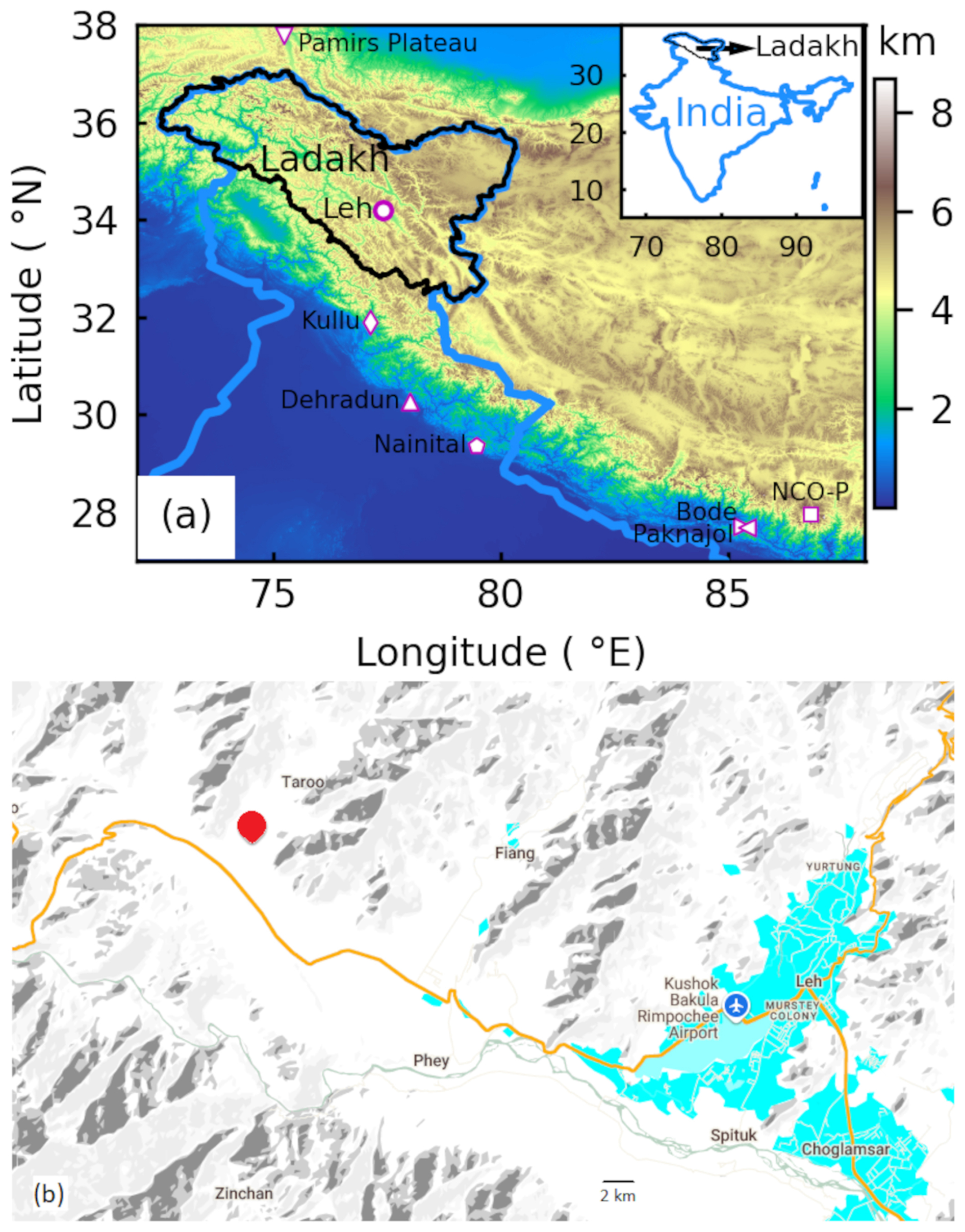
Figure 1(a) Elevation map of the northern Indian Subcontinent. The location of the measurement site (Leh, Ladakh) is marked as a magenta circle. Other nearby sites are also shown which are used for comparison of O3 variations. Inset in (a) shows a wider view, depicting Ladakh region in northern most part of India. (b) Zoomed map around measurement location, i.e., University of Ladakh (red symbol) and adjacent Leh town (big cyan patch). A highway is shown with an orange curve.
2.1 Study region and in situ measurements
Surface O3 measurements has been carried out since October 2024 at the University of Ladakh (34.185° N; 77.412° E; ∼ 3.4 ), which is ∼ 16 km (aerial distance) away from the Leh town (Fig. 1b; modified from https://maps.google.com, last access: 16 November 2026). No major local anthropogenic activity occurs within the radius of ∼ 2 km. Temperature, relative humidity, surface pressure and daily accumulated rain were observed in the range of −10 to 24 °C, 6 %–98 %, 651–668 hPa, 0–36.5 mm, respectively at Leh as per the India Meteorology Department. Temporal variations in these meteorological parameters are shown in Fig. S1 in the Supplement. A few days (23–28 October 2024) of wind measurements were also carried out at the study site. The synoptic winds at 600 hPa, obtained from the European Centre for Medium-Range Weather Forecasts (ECMWF) Reanalysis 5 (ERA5; Hersbach et al., 2020), show jumbled winds (owing to the complex topography) with downdrafts during winter and pre-monsoon. However, north-westerly or westerly winds prevailed without downdrafts during the monsoon and post-monsoon seasons (Fig. S2). Further details on the climate of the Leh region are available elsewhere (e.g., Chevuturi et al., 2018).
In situ O3 measurements have been carried out using a factory-calibrated (NIST Traceable) ultraviolet (UV) photometric analyser (2B Tech, USA; Model: 106-L). Air samples were drawn from a height of ∼ 10.6 m above the ground using a Teflon tube through a 5 µm non-reactive polytetrafluoroethylene hydrophobic dust filter. The analyser measures O3 based on the absorption of UV radiation at ∼ 245 nm applying the Beer–Lambert law. The lower detection limit, linearity, and minimum response time are 3 ppbv, ± 1 %, and 20 s, respectively. The measurement uncertainty of the UV photometric analyser is reported to be approximately 5 % (Tanimoto et al., 2007). The instrument was continuously operated in a temperature controlled environment maintaining its permissible limits of temperature (0–50 °C). Inter-comparison of this instrument with a calibrated O3 analyser (Thermo Scientific, USA) using a common inlet system showed an excellent agreement (Fig. S3), prior to its deployment at the site. Measurements were recorded at an averaging interval of 5 min and were converted to hourly averages for the analysis.
2.2 Satellite observations
To interpret the observed O3 variability and assess long-term changes, the study utilized tropospheric columns of HCHO and NO2, along with total column CO, derived from TROPOMI (TROPOspheric Monitoring Instrument) aboard the polar-orbiting Sentinel-5 Precursor satellite (equator crossing time: ∼ 13:30 LT). NO2, CO and HCHO are derived from the spectral measurements in 405–465 nm, around 2.3 µm and 328–359 nm, respectively. The retrieval algorithms and validations have been described in previous literature (Borsdorff et al., 2018; De Smedt et al., 2018; Landgraf et al., 2016; Van Geffen et al., 2022). Offline level-3 products of NO2 and HCHO are available at spatial resolution of 3.5 × 5.5 km2 and CO is available at spatial resolution of 7.5 × 5.5 km2 (across × along track) since 28 June 2018. Data with quality assurance greater than or equal to 0.50 (0.75 for NO2) were obtained from Google Earth Engine, https://code.earthengine.google.com (last access: 16 November 2026).
To consider the possible influences of cloudiness on atmospheric chemistry, we have also utilized data from the Indian geostationary satellite, INSAT-3DS (Indian National Satellite – 3D second repeat). Level-2B cloud mask (L2B CMK) is derived from three infrared channels of the imager (Mid-wave infrared: 3.9 (3.80–4.00) µm, Thermal infrared-1: 10.8 (10.3–11.3) µm, Thermal infrared-2: 12 (11.5–12.5) µm) and data is available at 30 min intervals with a spatial resolution of 4 km. Details of the algorithm can be found here: https://mosdac.gov.in/docs/INSAT_3D_ATBD_MAY_2015.pdf (last access: 16 November 2026). We considered 25 pixels with a central pixel lying over the study site during the morning hours (08:30–14:00 IST – Indian Standard Time) and summed up the number of cloudy pixels on a daily basis. These daily sum values were used to obtain the monthly averages of the number of cloudy pixels.
2.3 Reanalysis datasets
Surface O3 and stratospheric ozone tracer from the Copernicus Atmosphere Monitoring Service (CAMS; Inness et al., 2019), available at 3 h interval with a spatial resolution of 0.75° × 0.75°, have been used to analyse the seasonal pattern, stratospheric contribution, and long-term trend during the 2015–2024 period. This is the fourth generation ECMWF global reanalysis of atmospheric composition (EAC4). Monthly mean vertical wind from ERA5 – ECMWF Reanalysis 5 (hourly interval; 0.25° × 0.25°; Hersbach et al., 2020) is used to understand the prevailing downdraft/updraft. Both CAMS and ERA5 utilise the ECMWF Integrated Forecasting System (IFS) with 4D-var data assimilation. CAMS employs a fully integrated chemistry framework based on the Carbon Bond (CB05) mechanism, comprising 54 species and 126 reactions (Huijnen et al., 2010), with assimilation of satellite observations. Further details of the evaluation of these reanalyses can be found elsewhere (Harithasree et al., 2024; Inness et al., 2019; Park et al., 2020). The CAMS time series at grid, 33.75° N; 78.25° E, closest to the study region is considered for the analysis.
2.4 Global model simulations and source tagging
We have utilized output from dual-source tagging-enabled global model CAM4-Chem (Community Atmosphere Model with Chemistry version-4; Butler et al., 2020) available for a 19-year period of 2000–2018, as described in Ansari et al. (2025) and Nalam et al. (2025). Hourly surface O3 mixing ratios along with its tagged contributions have been analysed at the grid cell, closest to the observation site. The model calculates O3 contributions from both NOx as well as VOC (including CO and CH4) through two separately tagged simulations. Geographic definitions of specific source regions are shown in Fig. S4. Monthly varying gridded anthropogenic emissions of NOx, CO, SO2, NH3, OC, BC and NMVOCs, input to the model, are based on the HTAP (Hemispheric Transport of Air Pollution) v3.1 global mosaic inventory for the 2000–2018 period (Crippa et al., 2023). Biogenic emissions are included from the CAMS-GLOB-BIO-v3.0 (Sindelarova et al., 2022) while biogenic soil NOx is specified as in Tilmes et al. (2015). Biomass burning emissions are prescribed from GFED-v4 inventory (Van Der Werf et al., 2010). The model has a horizontal resolution of 1.9° × 2.5°, with 56 vertical levels extending up to model top at approximately 1.86 hPa. The model setup and evaluation results assessing the same global simulations have been discussed in recent studies over North America and Europe (Ansari et al., 2025), East and Southeast Asia (Lu et al., 2025), and the global troposphere (Nalam et al., 2025). In this analysis, stratospheric O3 (O3s) contribution to surface O3 has been considered from CAMS reanalysis as this adjustment improved the agreement of CAM4-Chem simulation with observations. For this, CAM4-Chem estimated O3s has been subtracted from CAM4-Chem estimated O3 and then CAMS derived O3s has been added.
Here, O3 source attribution is performed using the TOAST 1.0 tagging system developed by Butler et al. (2018). The system introduces additional tagged species into the model's chemical mechanism and physical process routines, allowing them to be transported and processed alongside the original chemical species that represent the total baseline emissions. Two parallel simulations are conducted: one tracking the contributions of NOx emissions and the other tracking those of volatile organic compounds (VOCs). In each simulation, tagged species represent emissions from a specific source region or sector, with the corresponding tag indicated by a variable suffix (see Table S1 in the Supplement and Fig. S4 for the regional and sectoral definitions). For example, NO_NAM, NO_SAS, and NO_EAS represent NO emitted from North America, South Asia, and East Asia, respectively. As tagged species participate in chemical reactions, their source labels are propagated through the reaction pathways and ultimately assigned to the resulting O3 molecules. Thus, O3 formed from NOx originating in South Asia is represented as O3_SAS in the NOx-tagging simulation, while O3 formed through the oxidation of VOCs originating in the same region is represented as O3_SAS in the VOC-tagging simulation.
Separate simulations are necessary because O3 formation involves interactions between NOx and VOCs that may originate from different regions or sectors. A single O3 molecule can therefore be associated with both a NOx source and a VOC source; the two simulations independently quantify these contributions. The tagging system also distinguishes between NO2 formed through the oxidation of NO and NO2 formed through O3 titration. When a tagged NO molecule (e.g., NO_NAM) reacts with an O3 molecule carrying a different regional tag (e.g., O3_SAS), the resulting NO2 is assigned the O3 molecule's tag (NO2_SAS), rather than the NO molecule's tag (NO2_NAM). This convention preserves the source attribution of O3 consumed through titration and distinguishes it from NO2 produced through NO oxidation. Further details of the tagging methodology and simulation configurations are provided by Ansari et al. (2025) and Butler et al. (2018).
Note that since the latest emissions for 2024–2025 are unavailable, we have used simulation results from previous years, 2009–2018, as climatological mean.
2.5 Regional model simulations
We have performed regional-scale numerical simulations of meteorological parameters and atmospheric composition at spatial resolution of 12 km × 12 km, by applying the Weather Research and Forecasting model coupled with Chemistry (WRF-Chem; Grell et al., 2005; Skamarock et al., 2019) version-4.5.1. Simulations have been conducted for 2 full months, February representing winter and September representing monsoon. Meteorological fields input to the model are based on ERA5 reanalysis (Hersbach et al., 2020). For parametrizing cumulus physics and boundary layer processes, the Grell 3D (Grell and Dévényi, 2002) and Yonsei University (Hong et al., 2006) schemes, respectively, have been utilized. To limit errors in large-scale meteorological and dynamical variations, the temperature, horizontal winds, and water vapour have been nudged at all vertical levels with nudging coefficients of 3 × 10⁻⁴ s−1 (Otte, 2008; Sharma et al., 2017). Here, nudging coefficient is kept lower than previous studies over South Asia (6 × 10⁻⁴ s−1; Kumar et al., 2012a, b), to minimise the potential suppression of fine-scale local circulations simulated by the WRF dynamics.
Anthropogenic emissions are based on the EDGAR (Emissions Database for Global Atmospheric Research) inventory for year 2015 (Crippa et al., 2020; Mogno and Marvin, 2022) and fire emissions are based on FINN v2.5 (Fire INventory from NCAR (National Center for Atmospheric Research); Wiedinmyer et al., 2023) for year 2021. Natural biogenic emissions are computed online using the MEGAN (Model of Emissions of Gases and Aerosols from Nature Guenther et al., 2006). Gas-phase chemistry is represented by the MOZART (Model for Ozone and Related chemical Tracers) mechanism (Emmons et al., 2010) and aerosols are calculated using the MOSAIC (Model for Simulating Aerosol Interactions and Chemistry; Zaveri et al., 2008). Initial and lateral boundary conditions for the chemical fields have been provided from the WACCM (Whole Atmosphere Community Climate Model) global simulations (Gettelman et al., 2019). We have noted a systematic overestimation of O3 in remote environments of India and that reducing inflow from the global model by about 40 % leads to better agreement between WRF-Chem output versus measurements. Comparison of model simulated surface O3 with measured O3 shows a good agreement (r = 0.4–0.8) with smaller negative bias of 7–9 ppbv (Fig. S5). This shows the model's capability to capture the observed variations reasonably and hence it can be used to gain deeper insights into the various processes contributing to observed variations. The tendency terms in the WRF-Chem (Barth et al., 2012; Girach et al., 2017) have been analysed to quantify the roles of various chemical and dynamical processes in influencing O3 variations. More detailed description of the WRF-Chem model (Grell et al., 2005) and its evaluations and diverse applications over Indian subcontinent can be found elsewhere (Ghude et al., 2025; Girach et al., 2017; Kumar et al., 2012a, b; Sharma et al., 2017).
Here, EDGAR inventory for the year 2015 has been used due to the lack of up-to-date emission changes over this region in inventories. As discussed in Sect. 3.7, the anthropogenic emissions are increasing over the study region and hence actual emission could be different. Nevertheless, here we use WRF-Chem simulation only to infer the main processes influencing the diurnal and day-to-day changes in O3.
2.6 Indices for air quality assessment
Maximum Daily 8 h Average ozone (MDA8) is related to short-term health impact with a threshold value of 100 µg m−3 set by the World Health Organization (WHO, 2021) as well as by India's National Ambient Air Quality Standards (NAAQS; https://cpcb.gov.in/uploads/National_Ambient_Air_Quality_Standards.pdf, last access: 16 November 2026). MDA8 is a maximum value of 8 h running averages obtained using hourly O3 on a daily basis. Hourly O3 mixing ratio (ppbv) is converted to concentration (µg m−3) using measured pressure and temperature (Fig. S1). To quantify health impacts due to long-term O3 exposure, another metric OSDMA8 (ozone season daily maximum 8 h average) has been estimated, which is basically the annual maximum of 6 month running mean of MDA8 (GBD 2019 Risk Factors Collaborators, 2020). The risk to vegetation/crops and ecosystems can be assessed based on the estimation of four different metrics: M7 (7 h Mean, averaged during daytime, 09:00–16:00 IST), AOT40 (Accumulated exposure to Ozone above a threshold of 40 ppbv), SUM06 (the sum of all hourly O3 concentrations ≥ 0.06 ppm) and W126 (hourly concentrations weighed by a sigmoidal weighting function). AOT40, SUM06 and W126 are calculated for daylight hours, 07:00–18:00 IST (Fuhrer et al., 1997; Hogsett et al., 1988; Lee et al., 1988; Lefohn and Runeckles, 1987; Mills et al., 2007). SUM06 and W126 better represent the crop loss as found in the experimental studies in the US (Kaylor et al., 2023). Threshold value or safe limit for AOT40 is 1 ppmv h as defined by UNECE (United Nations Economic Commission for Europe), 1996 (Fuhrer et al., 1997; https://www.umweltbundesamt.de/system/files/medien/4038/dokumente/manual_complete_english.pdf, last access: 16 November 2026). There are no thresholds defined for M7, W126 and SUM06 as lower levels of O3 can also have adverse impacts on vegetation. Formulae for these exposure indices are given in Sect. S1 in the Supplement.
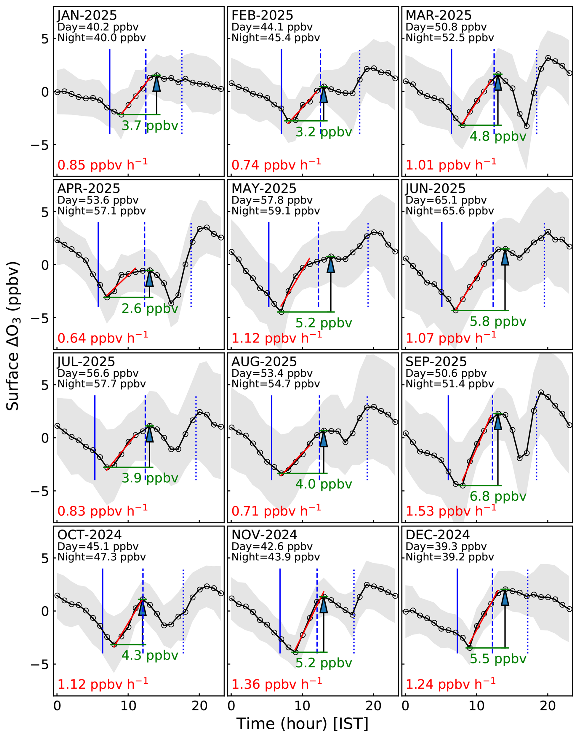
Figure 2Monthly mean diurnal variations of ΔO3 over the Trans-Himalaya. The shaded grey region shows the standard deviation. The red line shows the linear fit over the 5 h period from the morning minimum. The slope representing net O3 production rate (ppbv h−1) is given in red colour font. Total daytime build-up, noontime maximum minus morning minimum, is marked in green colour. Vertical blue lines represent sunrise (continuous line), local noon (dashed line) and sunset (dotted line). Mean values of daytime and nighttime O3 are also mentioned. Here, daytime is defined as 2 h after sunrise until 2 h before sunset. Likewise, night is defined.
3.1 Diurnal variations and daytime O3 build-up
ΔO3 for a given day is obtained by subtracting the daily mean from the hourly values of the corresponding day. The mean diurnal patterns of ΔO3 for different months are shown in Fig. 2. The average diurnal variations for different seasons are shown in Fig. S6. The diurnal patterns of ΔO3 are observed to be quite unique in this region, nevertheless, similar across different months, with three important features: (a) nighttime (22:00–07:00 IST) decline, (b) build up after sunrise to the noontime (07:00–14:00 IST) followed by decline in the afternoon (13:00–17:00 IST), and (c) increase in the evening (17:00–20:00 IST). Noontime peak values are comparable or lower than midnight/nighttime values. Since daytime values are generally lower than nighttime values by 0–3 ppbv, there appears to be a net chemical loss on a daily scale. However, to a certain extent, this shows that O3 loss occurring during nighttime (20:00–06:00 IST) is partially compensated by daytime photochemical production. The day-to-day variability, as represented by the standard deviation (shaded region in Fig. 2) is seen to be larger (3–5 ppbv) during monsoon, as compared to other seasons (1–4 ppbv). This is likely due to sporadic mixing of different air masses owing to changes in meteorological conditions, especially day-to-day changes in convection strengths during July to September (Romatschke and Houze, 2011).
The rate of increase from morning (07:00–09:00 IST) to afternoon (12:00–14:00 IST) is estimated as the slope of linear fit to five successive hourly values from the morning minimum value, which ranged between 0.6–1.5 ppbv h−1. The photochemical O3 build-up, estimated as the noontime maximum minus morning minimum, ranged from 2.6–6.8 ppbv. O3 concentration starts increasing in the morning 1.5–2 h after sunrise. The O3 curve attains its peak 0–2 h after the local noon (zenith). The evening increase is mostly before sunset (Fig. 2). Interestingly, the evening O3 peak is higher than the noontime peak for most of the months, except during winter.
It is important to note that the study region experiences a photochemical O3 build-up after sunrise, a feature typically unseen over other high-altitude sites such as Nainital (1.9 , Sarangi et al., 2014), Mount Abu (24.6° N, 72.7° E, 1.7 , Naja, 2003), Mount Fuji (35.4° N, 138.7° E, 3.7 ; Tsutsumi et al., 1994), Ooty (11.4° N, 76.7° E, 2.5 ; Udayasoorian et al., 2013) and Ponmudi (8.76° N, 77.11° E, 1 ; Ajayakumar et al., 2024). In particular, the ΔO3 diurnal patterns show decline after the sunrise or remain nearly stable throughout the day over high-altitude sites in the Himalaya (Nainital and NCO-P; Fig. S6). Afternoon time O3 enhancements at Nainital was attributed to transport of pollutants from adjoining low-altitude IGP (Indo–Gangetic Plain) through boundary layer mixing. This comparison suggests that unlike the central/eastern Himalaya, there are significant precursors over the Trans-Himalaya which can result in observed photochemical O3 production in the presence of intense solar radiation. Note that due to its higher elevation, the Trans-Himalaya region receives more intense solar radiation (7 ) than central Himalayas or other lower elevation sites (5.6 ) in India (Santra, 2016). Note that here O3 production rate is slower (0.6–1.5 ppbv h−1) than that in polluted valleys and foothills of the Himalaya (4.7–10.1 ppbv h−1; Ojha et al., 2019). For further insight into photochemistry, we analysed co-located satellite observations to identify O3 formation regime which are discussed later in Sect. 3.4.
Qualitatively, the models reproduce the diurnal ΔO3 pattern, except missing the late evening-time enhancement. Quantitatively, diurnal amplitude in CAM4-Chem as well as WRF-Chem models matches with the observations (∼ 3 ppbv) during February. Both models do show an increase in diurnal amplitude in September but overestimate its magnitude (12–15 ppbv) than observed values (7 ppbv). However, chemistry appears much more intense in the CAMS reanalysis particularly during September. Our results suggest that simulations from CAM4-Chem and WRF-Chem may be analysed for deriving further insights into the factors governing O3 magnitude and variations. Few other limitations which we are reporting here, although are not quite surprising, would be useful for future improvements and fine-tuning of the models. It is likely that the evening surge is associated with mesoscale dynamics, transport of O3 rich air from higher altitudes due to mountain-valley circulation (Sarangi et al., 2014) or through other orographic influences unresolved even at high resolutions (Singh et al., 2021) in complex Himalayas. Alternatively, the afternoon dip (13:00–17:00 IST) could have been associated with local-scale dynamics, which could not be represented adequately in the model.
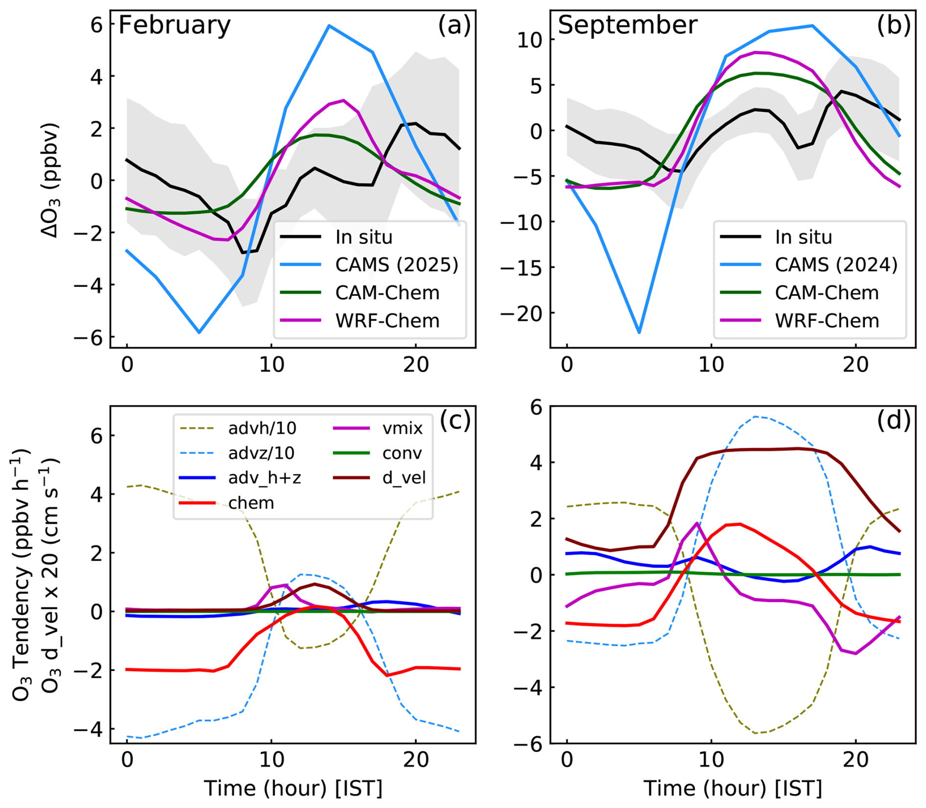
Figure 3(a, b) Comparison of observed diurnal ΔO3 variation at Leh with simulations from global (CAMS and CAM4-Chem) and regional (WRF-Chem) models. WRF-Chem inferred deposition velocity (d_vel) and mean tendencies due to different processes: horizontal advection (advh), vertical advection (advz), convection (conv), chemistry (chem), and vertical mixing (vmix) are shown in panels (c) and (d).
The tendency terms from WRF-Chem simulations have been analysed to infer the main processes governing O3 diurnal variation during two contrasting seasons (Fig. 3c and d). The daytime build-up during winter is linked with decreased chemical loss and increased contribution through vertical mixing in the morning hours (Fig. 3c). Small contributions from the advection are seen in the evening hours. Contrary to winter, larger photochemical production drives daytime increase of O3 during monsoon season (Fig. 3d). Interestingly, while vertical mixing positively contributes to enhanced O3 in the morning hours, it reduces O3 in the evening hours in the model. Positive advective contributions help to sustain O3 levels during the monsoon throughout the day, except near noontime. The deposition velocity of O3 is elevated during daytime, especially in the monsoon, but it is negligible during nighttime in both seasons. The results suggest higher depositional loss of O3 in summer as compared to the winter. A slow decrease in O3 during nighttime is due to chemical loss plus vertical mixing as seen by negative chemical tendencies during both seasons (Fig. 3c and d). Thus, the model fields provided key insights into the relative roles of different processes shaping O3 diurnal pattern, besides indicating the factors that may need improvements to reduce the model-measurement differences such as in late evening or night.
The diurnal pattern of O3 is also linked with the wind direction, which would transport different airmasses during the course of the day. To infer this effect, a few days of collocated measurements of wind and ΔO3 (23–28 October 2025) have been analysed (Fig. 4). While the lower O3 in the morning hours are associated with mainly wind direction 0–60° N, higher values are associated with the wind from 90–315° N (Northwest, southwest and southeast sectors) during noon to late night hours. Further, the standard deviation (Fig. 4c) estimated by following Yamartino, 1984 suggests significant variability in the wind direction. The climatologies of satellite observed precursors, NO2 and CO, also show relatively higher levels over valley regions of the Trans-Himalaya (Fig. 5a and c), indicating local emissions. Relatively higher anthropogenic activities including vehicular emission (note the national highway in valley region, south of the measurement site; Fig. 1b) is evident from the relatively higher concentration of NO2 and CO (Fig. 5d and f). Therefore, the noontime higher O3 or noontime build-up corresponding to wind directions 90–315° N (Fig. 4), is likely to be contributed by emissions in the adjoining areas (Fig. 5d an f; south and southwest of the measurement site). Tropospheric column NO2 over the observational site is in the range of ∼ 0.2–1.7 , which translates to the boundary layer mixing ratio of 0.1–0.9 ppbv with assumption that 90 % of tropospheric NO2 is within 1 km of boundary layer height. This would contribute to the observed daytime build-up of O3. In addition, there exists afternoon dip in O3 over the same wind sector which could be due to titration by fresh emissions. The lower O3 in the morning hours is likely to have minimal local influence as precursors are lower in the north of the study site (0–60° N; Figs. 4a, b and 5d, f). The higher NO2 in the east or southeast of the study site represents Leh town and its direct influence on the study site is unlikely due to mountains in-between (Fig. 1b). Additionally, the lower HCHO levels (proxy of VOCs) would limit the in situ photochemical production of O3 over the site. Nevertheless, further observations in the Trans-Himalaya related to chemical composition and dynamics would be needed for pinpointing the role of local emissions and fine-scale dynamical processes.
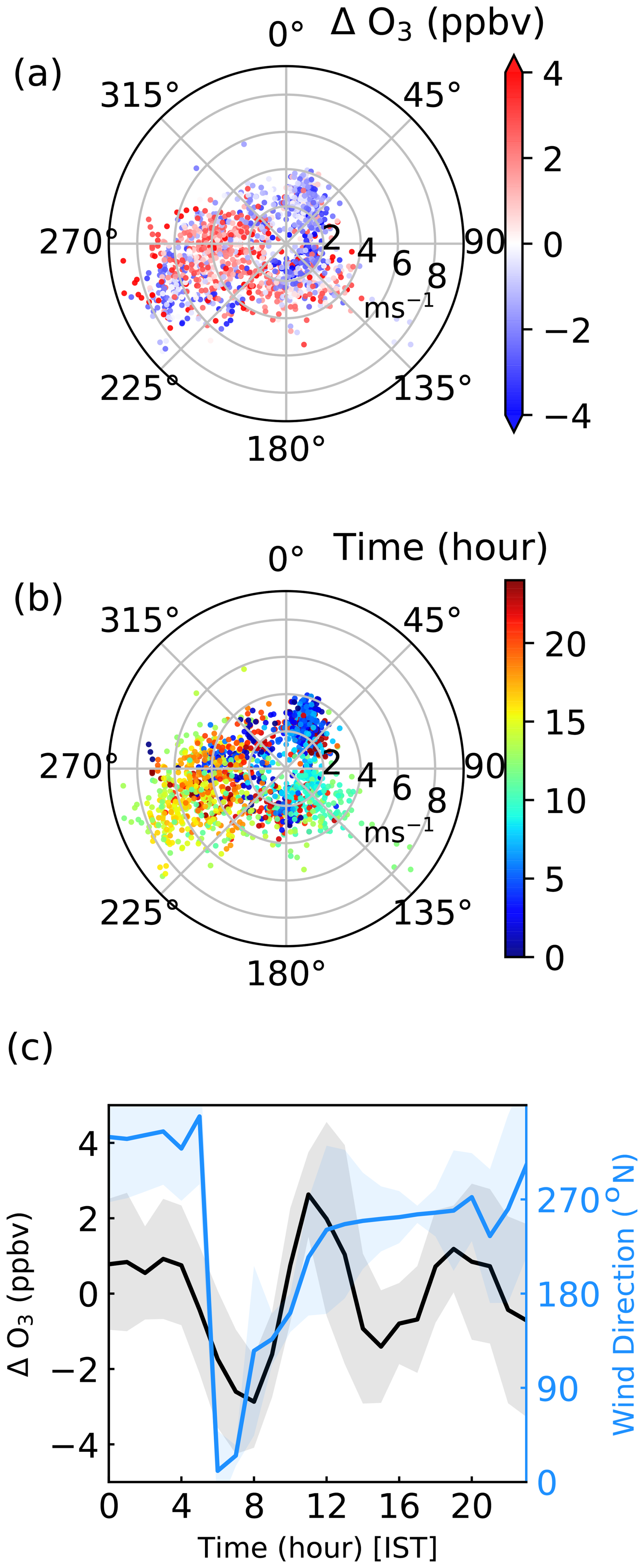
Figure 4Wind rose colour coded with ΔO3 and time (a, b) and diurnal variations in ΔO3 and wind direction (c) over the study region during 23–28 October 2024. Shaded regions in panel (c) represent standard deviation.
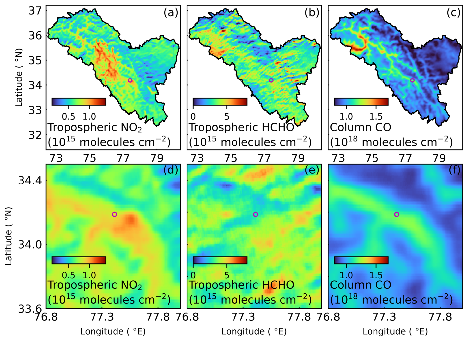
Figure 5Mean distribution of TROPOMI observed NO2, HCHO and CO over the study region during October 2018–September 2026. Magenta circle marks the study site. Panels (d)–(f) are the zoomed view around the study site.
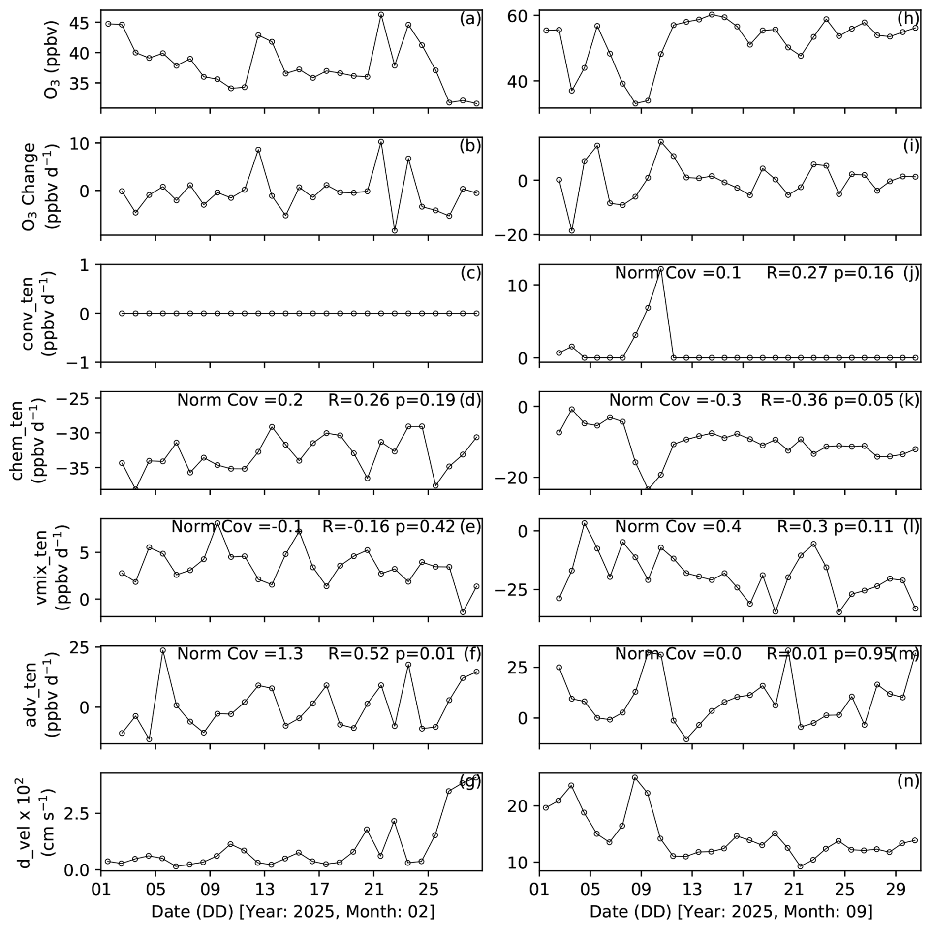
Figure 6Noontime O3 (13:00 IST), its changes with respect to the previous day, various tendencies and deposition velocity during representative months of winter (a–g) and summer monsoon (h–n) seasons. The y-axis labels, conv_ten, chem_ten, vmix_ten, adv_ten, and d_vel, represent O3 tendencies (ppbv d−1) due to convection, chemistry, vertical mixing, advection, and O3 deposition velocity (cm s−1). Correlation coefficient (R) and normalised covariance are between O3 change (ppbv d−1; b, i) and tendencies (c–f and j–m). Here, covariance is normalised with respect to variance in O3 change (b, i). The p value is also marked along with R.
3.2 Day-to-day variations and contributing processes
The day-to-day changes in noontime (13:00 IST) values of O3 and different tendency terms, as derived from the WRF-Chem simulation, are shown in Fig. 6. For this, change in O3 is obtained by subtracting values at 13:00 IST on (n−1)th day from value at the same time on nth day. Similarly, tendencies shown here are obtained the same way from WRF-chem simulated accumulated tendencies. Generally, the tendencies (difference between consecutive values of cumulative tendency at hourly interval) oscillate around a baseline reflecting embedded diurnal changes and the sum of all tendencies (conv_ten, chem_ten, vmix_ten, and adv_ten) represent the hourly net change in O3. Here, day-to-day changes in O3 have been analysed by estimating the tendencies at the daily scale (ppbv d−1; Fig. 6). To assess the role of different tendencies in changing O3, correlation coefficient and normalised covariance are also estimated between tendencies versus O3 change as mentioned in the figure. Day-to-day changes in noontime O3 are smaller in February (up to 10 ppbv d−1) compared to September (up to 20 ppbv d−1), as seen in Fig. 6b and i. Chemical tendencies are typically negative over this region (figure 6-d and k), being −30 to −40 ppbv d−1 in February but 0 to −10 ppbv d−1 in September (except during convective episode; 8–11 September). This indicates that the region acts as a net chemical sink of O3 during both the seasons, being a stronger sink during the winter season. The gradual nighttime (20:00–06:00 IST) declines seen in the observations (Fig. 2) also support the role of titration of O3. Monthly sum of hourly changes in observed O3 turns out to be negative during most of the months, except in January, March, June, and August (Fig. S7). This is consistent with the model-based inference that the region acts as a net chemical sink. Dynamics (convection plus advection) compensated more than the stronger chemical losses during 8–10 September, leading to overall O3 increase. Little variations in chemical losses in other days but strong anti-correlation in this period led to an overall negative correlation between chemical tendencies and O3 change in September.
The advection tendencies are generally positive and cause an increase in O3. Transport due to advection has a greater bearing on O3 change during winter, as inferred from the higher correlation and covariance (Fig. 6f; R=0.5, normalised covariance 1.3). In contrast, no single process dominates day-to-day O3 changes during monsoon. The contributions from multiple processes govern the O3 changes during monsoon.
Convection is not a key factor in general, except during a large increase in O3 during 8–11 September when it exceeded 10 ppbv d−1 (Fig. 6c and j). Deposition velocity also shows significant variations (February: 0.01 ± 0.01 cm s−1; September: 0.15 ± 0.04 cm s−1) with enhancements during convective episodes (e.g., around 9 September 2025).
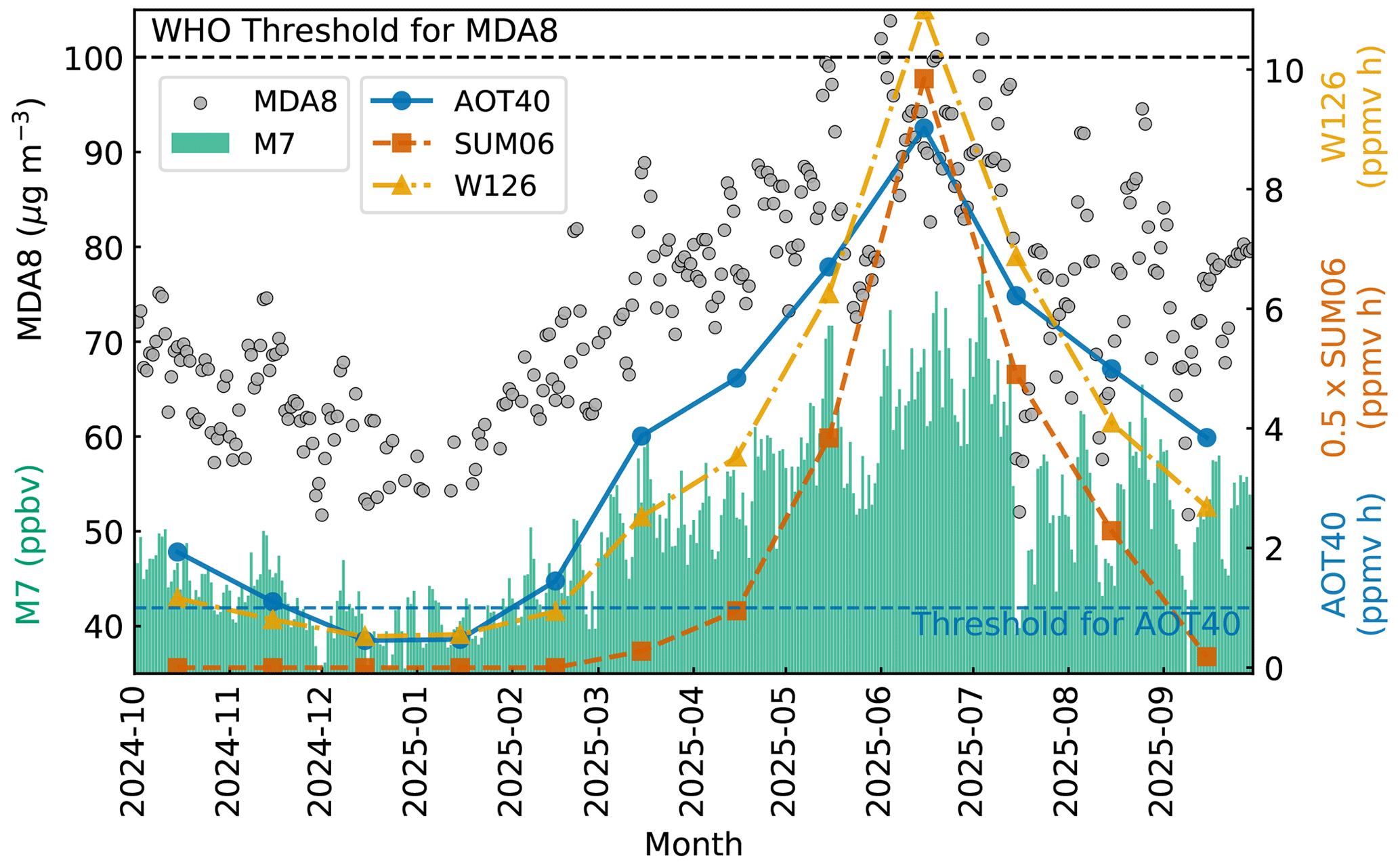
Figure 7Variations in various ozone exposure metrics during the study period. Threshold values of MDA8 (100 µg m−3) and AOT40 (1 ppmv h) are indicated by horizontal dashed lines.
3.3 Air quality impacts
Our first systematic O3 measurements can provide insights into O3 impacts on the public health and vegetation over the Leh region. In this regard, several standard and widely applied exposure metrics have been estimated and compared with the thresholds (Fig. 7). All O3 exposure indices are observed to be higher during May–July, peaking in the month of June. MDA8 values ranged from 52–104 µg m−3 (37–80 ppbv) during the study period. MDA8 values are very close to the threshold of 100 µg m−3, with 33 d experiencing values above 90 µg m−3 and thrice exceeding the threshold during May–July. OSDMA8 is 82 µg m−3 (or 61 ppbv), which is significantly higher than the minimum risk level of 32.4 ppbv (Turnock et al., 2025). The AOT40 values are above the threshold of 1 ppmv h except during November–February. Annual cumulative values of AOT40, SUM06 and W126 are estimated to be 44.9, 44.6, and 40.9 ppmv h, respectively. Magnitudes of these indices are comparable with those over the US and South Korea (Kaylor et al., 2023; Lee et al., 2023). AOT40, SUM06 and W126 have been reported to range between 0–5, 1–20, and 1–15 ppmv h, respectively, over China during the crop growing season of winter (Jiao et al., 2025), which are comparable or slightly higher than the present study region. Increase in AOT40 between 13 to 17 ppmv h is also reported over the Indian region during wheat growing season (January–March) of 2005–2021 (Anagha and Kuttippurath, 2026). With increasing global baseline O3 and anthropogenic emissions across South Asia, our results indicate likelihood of more frequent exceedance of air quality standards in this region. In this regard, O3 formation regime (Sect. 3.4) and long-term trends (Sect. 3.7) have been analysed for informing the policies.
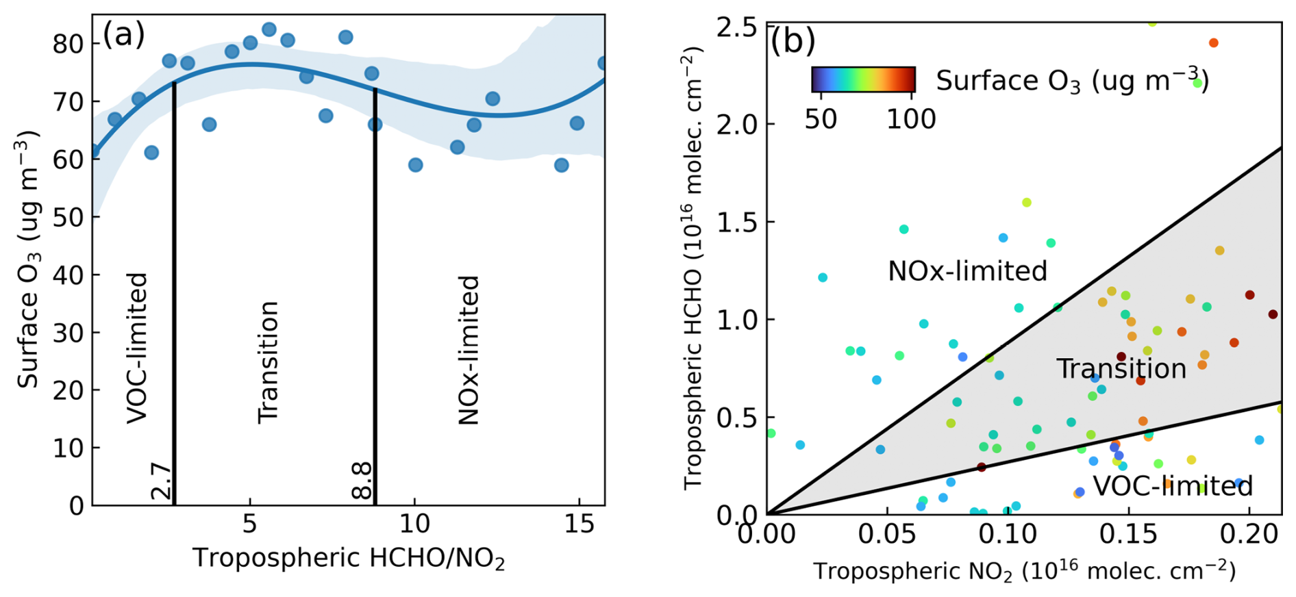
Figure 8(a) Variations of surface O3 with collocated tropospheric ratio over the study region. Blue curve represents the 3rd order polynomial fit with 95 % confidence level (shaded region). (b) Scatterplot of tropospheric HCHO versus NO2 colour-coded with surface O3. Black lines in panels (a) and (b) demarcate O3 formation regimes, as labelled.
3.4 O3 formation regime
TROPOMI observations of tropospheric HCHO and NO2 have been used to determine the threshold values of the ratio to demarcate NOx and VOC-limited regimes suitable for the study region, following the literature (Jin et al., 2017; Martin et al., 2004). TROPOMI observations at a single pixel strictly co-located with ground-site are considered for the spatial co-location. Surface O3 values are averaged over a ± 15 min time window with respect to the satellite overpass (i.e., 30 min centred on the overpass time). The ratio is divided into 400 bins, and corresponding averages of O3 are fitted with a 3rd order polynomial as shown in Fig. 8a. Since the peak of the fitted curve is the central value in the transition regime, i.e., ridge of O3 isopleths, a slope from −3 to +3 of the fitted curve demarcates the VOC-limited versus NOx-limited regimes (Ren et al., 2022), corresponding to ratios of 2.7 and 8.8, respectively (Fig. 8a). Therefore, the values less than 2.7 represent a VOC-limited regime, whereas the values higher than 8.8 represent NOx-limited regime. Most of the higher values of O3 lie in the transition regime (Fig. 8b) suggesting that the O3 formation corresponding to higher values is contributed by both NOx and VOCs, and hence the effective mitigation will require reductions in both NOx and VOCs. In addition, since the O3 levels are particularly higher during May–July (Fig. 7), when ratio suggests prevalence of “relatively” fresh airmasses (compared to winter season; see Fig. S8), reduction in regional emissions in addition to local emissions would be essential to contain the O3 level within safe limits.
Here, it is worth mentioning that while satellite-retrieved ratios do provide insights into the chemical regimes, the inferences could have uncertainties. In this regard, particularly important factors include (a) higher retrieval noise under low concentrations over mountain region, which could result in uncertainty by > 100 % in ratio, (b) inherent chemistry assumption leading to 20 % standard error due to inaccurate description of the ROx–HOx cycle, (c) column-to-boundary layer translation, and (d) limited representativeness due to coarse spatial resolution missing sharp gradients in concentration across the satellite pixel (Acdan et al., 2023; Souri et al., 2023). Few studies have reported positive biases of ∼ 26 % and 9.5 % in TROPOMI HCHO and NO2, respectively for cleaner regions (HCHO < 2.5 × 10¹⁵ and NO2 < 2 × 10¹⁵ ) (De Smedt et al., 2021; Pasternak et al., 2026). Thus, further in situ measurements would be needed for validation of the results derived from satellite retrievals for this environment having strong heterogeneity in topography and tracer's distribution.
3.5 Seasonal variation: role of stratospheric intrusion and photochemistry
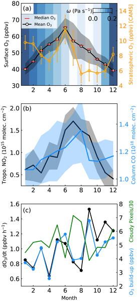
Figure 9 shows the seasonal variations of observed O3 and related parameters derived from reanalysis and satellite observations over the study region. O3 levels are lower during winter (39.2 ± 3.9 ppbv in December), increase in spring and attain maximum in June, just before the summer monsoon (65.2 ± 5.8 ppbv). Note that since summer monsoon onset is late, July rather than June, here monsoon period is from July to September (Bhan et al., 2015). The amplitude of the observed O3 seasonal cycle is 26 ppbv. CAMS derived O3s climatology shows its peak (11.4 ppbv) during June explaining about 18 % of the seasonal maximum of O3 over this region (Fig. 9a). This result is broadly consistent with more stratospheric intrusions over the Tibetan Plateau/China in the month of June (Liao et al., 2025). The stratospheric contribution is also substantial in winter (8–10 ppbv) but lower during other seasons (5–6 ppbv). Vertical wind at 650 hPa (close to the observed surface pressure of 651–668 hPa; Fig. S1) from ERA5 shows that the study region experiences downdraft consistently, except during the monsoon (see background colours in Fig. 9a). Strong downdrafts during winter with higher potential vorticity (5–10 × 10−6 ; Fig. S9) provide conducive conditions for downward transport of O3-rich air, in line with the analysis of CAMS O3s. During June 2025 when O3 peaked, potential vorticity remained above 2 × 10⁻⁶ suggesting the presence of stratospheric influence. The spatial distribution of O3s (not shown here) suggests that its enhanced contribution during June is not due to direct downward transport, instead it is due to horizontal transport from the Tibetan Plateau region. Stratospheric intrusions have been shown to increase surface O3 over Tibetan Plateau (e.g., Liao et al., 2025) with which this model-based inference is consistent.
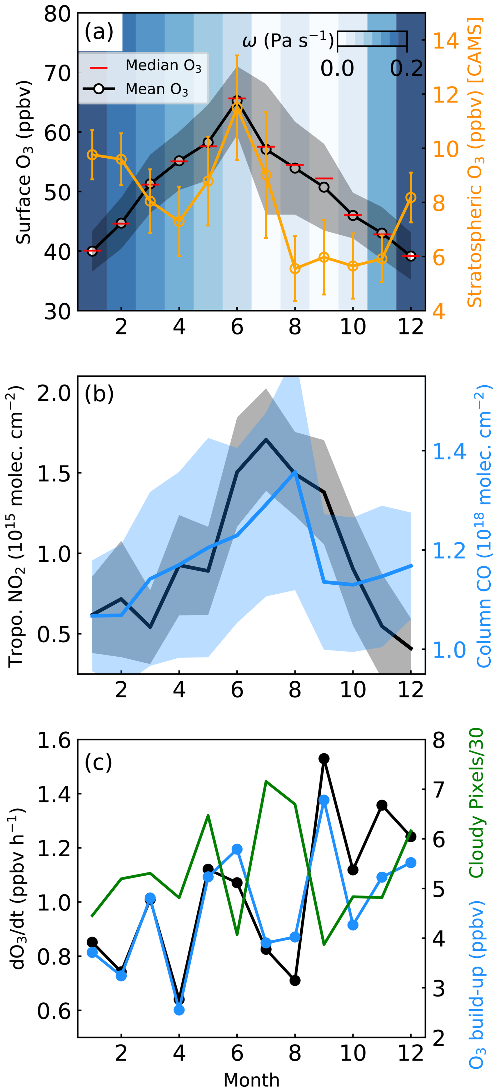
Figure 9Seasonal variation in (a) observed O3, vertical wind, and stratospheric O3 tracer (O3s), (b) satellite-derived tropospheric column NO2 and total CO column, and (c) observed rate of O3 increase (), daytime O3 build-up, and number of cloudy pixels derived from INSAT-3DS (08:30–14:00 IST) over the Leh region. All parameters are for the measurement period (October 2024–September 2025), except O3s for which climatology (2015–2024) is shown. The shaded region in panel (b) shows the standard deviation. Here, O3 build-up is the same as in Fig. 2.
Tropospheric NO2 and total CO columns from TROPOMI over the study region show higher values (NO2: 1.4–1.7 × 10¹⁵ ; CO: 1.2–1.4 × 10¹⁸ ) during monsoon (Fig. 9b). ratio peaks during June–July (Fig. S8) suggesting presence of photochemically “fresh” airmass likely transported from nearby regions, besides local emissions. The tourist activities are generally higher during summer (May–September) peaking in June, as compared to winter (Dolma, 2020). Larger abundances of the precursors in presence of intense solar radiation provide conducive conditions for photochemical O3 production during June. Figure 9c shows that higher rate of increase in O3 (: 1.1–1.5 ppbv h−1) and O3 build-up (6–7 ppbv; Fig. 2) during June and September but lower values during July–August (0.7–0.8 ppbv h−1; ∼ 4 ppbv) despite availability of precursors (Fig. 9b). The average number of cloudy pixels during morning hours (08:30–14:00 IST) obtained from INSAT-3DS shows more frequent cloudy conditions during July–August, which suppress the photochemistry leading to weaker noontime build-up. In addition, rain events during July–August (Fig. S1) would have washed out the precursors, inhibiting the O3 production.
O3 seasonal variation observed at Leh is compared with those at seven stations across Himalaya (Kullu, Dehradun, Nainital, Paknajol, Bode, NCO-P, and Pamir Plateau; marked in Fig. 1a), as shown in Fig. 10a. Monthly mean values are adopted from the literature (Cristofanelli et al., 2010; Harithasree et al., 2024; Mahata et al., 2018; Putero et al., 2015; Sarangi et al., 2014; Sharma et al., 2013; Yongde and Xinchun, 2025). O3 at Leh peaks in June, unlike other Himalayan sites where it peaks during pre-monsoon season (April–May) except over the Pamir Plateau (Yongde and Xinchun, 2025). Similar to the aforementioned regions, the pre-monsoon peak is ubiquitous in the Gangetic region or northern Indian subcontinent, owing to the regional pollution and intense solar radiation (Lal et al., 2017; Ojha et al., 2022). It is important to note that central Himalaya and its foothills are influenced by transport of precursors from the IGP during pre-monsoon, causing a peak in the seasonal pattern (Kumar et al., 2010; Sarangi et al., 2014). The O3 level reduces by a large magnitude of 10–25 ppbv during summer monsoon, with reference to pre- and post-monsoon values (dotted line in Fig. 10a), over most of the sites. The dotted line is derived by connecting pre-monsoon to post-monsoon months. Pre-monsoon month is chosen just before sharper monsoonal decline (April, May or June) and post-monsoon month (September, October or November) is chosen as corresponding to the peak after the monsoonal trough. The influence of the monsoon is absent or negligibly small over Leh as well as Pamir Plateau. In addition to the difference in the timing of the seasonal peak, the absence of strong monsoonal reduction is another key feature of the Trans-Himalaya.
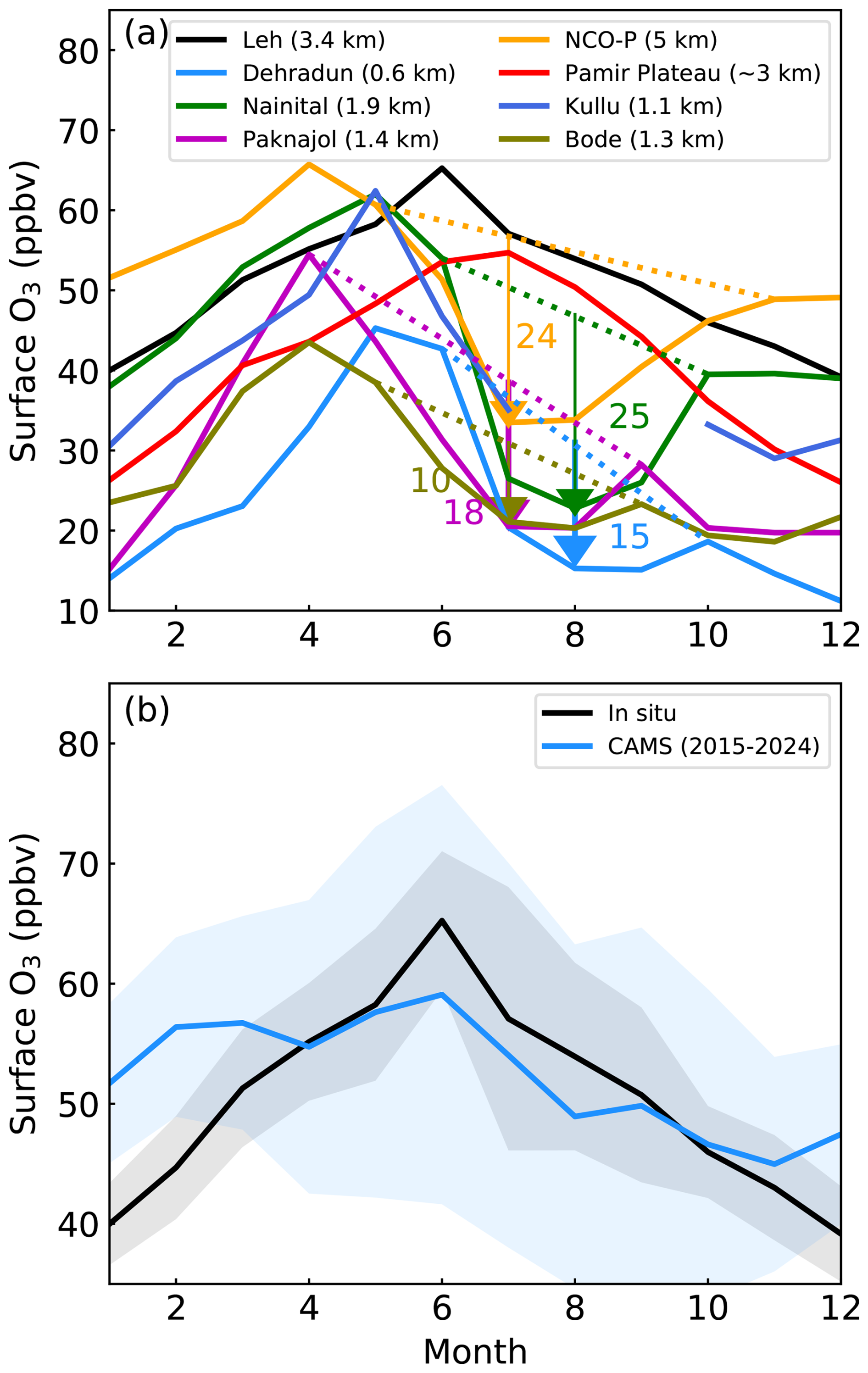
Figure 10(a) Comparison of O3 seasonal cycle over Leh with observations in the Himalaya, its foothills and Pamir Plateau. The altitudes of the sites are shown in the legend. Numbers in different colours show the approximate drop in O3 concentration during monsoon with respect to the hypothetical reference curve (dotted line) connecting pre- and post-monsoon values. (b) Seasonal variation of O3 from measurements and CAMS reanalysis over the study region. Stations shown in panel (a) are marked in Fig. 1a.
Figure 10b shows the monthly mean variations of observed O3 concentrations during 2024–2025 against the climatological mean O3 (2015–2024) derived from CAMS reanalysis for the study region. The CAMS-derived seasonal climatology agrees well with the observations except during winter. We do not have further parameters from the reanalysis for a deeper analysis of various contributing factors. To find the contributing factors responsible for the observed O3 variation, we analysed the results from the global chemistry–climate model as discussed in the following section.
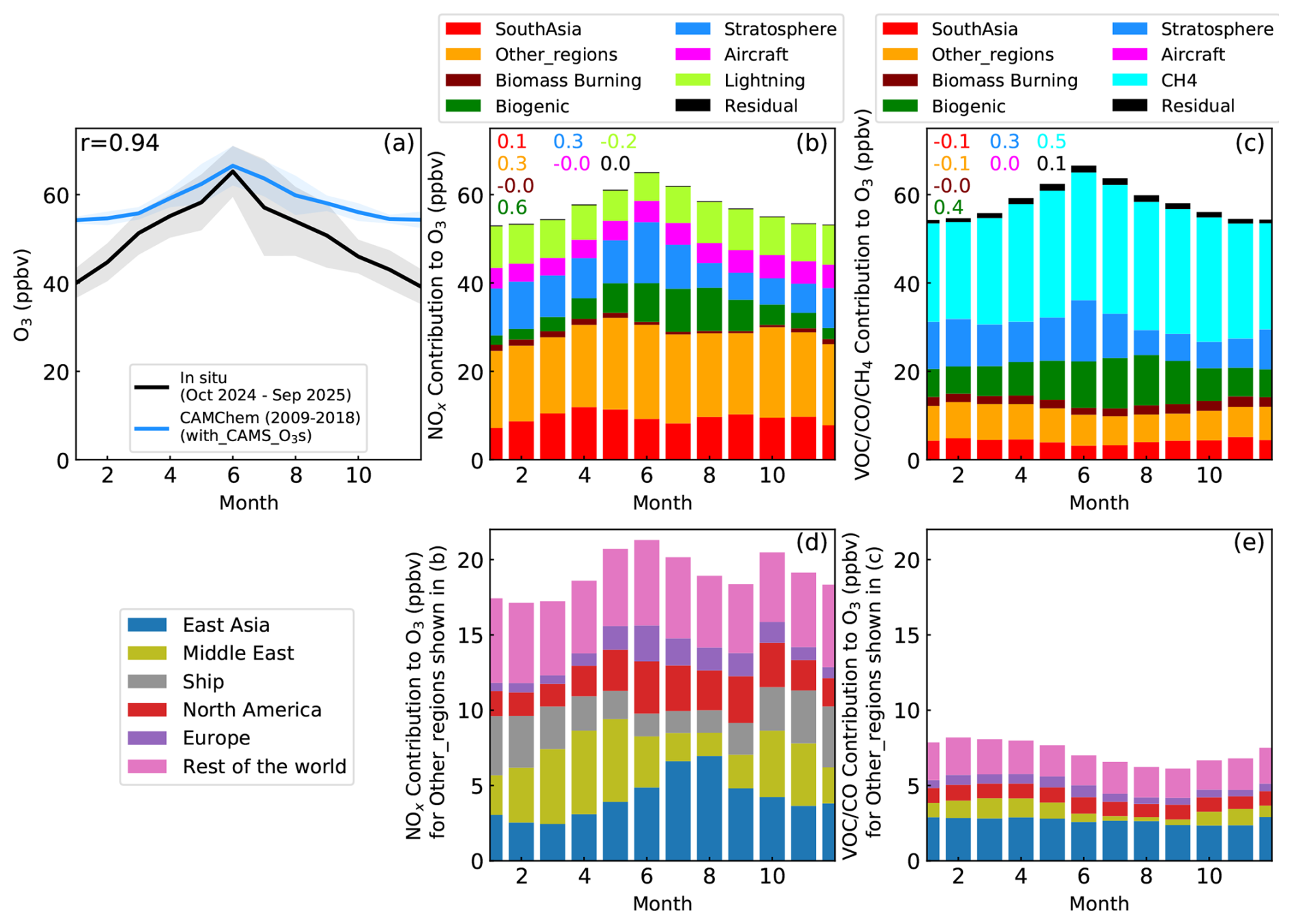
Figure 11(a) Seasonal variations of surface O3 from in situ measurements and from CAM4-Chem derived climatology (2009–2018) with stratospheric contribution updated by CAMS O3s, and CAM4-Chem derived contributions to O3 from (b) NOx sources and (c) VOC/CO/CH4 sources. Covariances of different sources normalised with variance in modelled O3 are marked with respective colours as in the legends in panels (b) and (c). The shaded region in panel (a) shows the standard deviations. Note that stratosphere in panels (b) and (c) refer to stratospheric O3, rather than contribution from stratospheric NOx or other precursors. Panels (d) and (e) provides further splits for different regions outside South Asia shown in panels (b) and (c). The definition of geographic regions is shown in Fig. S4. Here, “Rest of the world” in panels (d) and (e) includes contributions from all the regions (Fig. S4), other than those shown in legends.
3.6 Source attribution inferred from global model simulations
Figure 11 shows the observed and CAM4-Chem simulated seasonal variation of O3 concentrations over the Trans-Himalaya. The model broadly captures the seasonal pattern (r = 0.94) with a positive bias of 1–15 ppbv. The lowest bias is seen during the seasonal peak in June. Winter time overestimation (here, 10–15 ppbv) is commonly seen in most of the global models (Ansari et al., 2025; Gao et al., 2025 and references therein), including CAMS (Fig. 10b). A winter-time positive bias has also been reported for other regions in previous studies (Liu et al., 2022; Miyazaki et al., 2025). This high bias could be attributed to factors such as the inappropriate representation of temperature-dependent chemical and physical processes, and photolysis rates impacted by clouds. Unresolved topography could also contribute to bias as air masses are trapped in the shallow boundary layer during winter and the associated dynamics may not be captured at the coarse resolutions of the model. A recent study (Wild and Ryan, 2026) used an ensemble of atmospheric model runs with perturbed process parameters and found that the photochemical kinetic parameters and deposition rates, particularly over water and unvegetated surfaces (which largely define our study region), have been the largest source of uncertainty in simulating surface O3 (Emmerichs et al., 2021). More detailed investigations, especially model intercomparison exercises with perturbed process parameters, and not only with perturbed emissions, are required to pinpoint the causes of model biases (Carslaw et al., 2025).
O3 contributions are highly distributed across diverse NOx sources: global anthropogenic, South Asian, biomass burning, biogenic, lightning, and stratospheric O3, highlighting the background characteristic of this region. Interestingly, based on the NOx tagging (Fig. 11b), the largest contribution to O3 in CAM4-Chem model is seen from the anthropogenic sources outside the South Asia (Fig. S4), accounting for 30.9 %–36.6 % (17.1–21.3 ppbv). Other major contributions were from anthropogenic NOx emitted in South Asia (12.9 %–20.1 %; 7.1–11.9 ppbv), lightning (9.5 %–17.3 %; 6.3–9.4 ppb), and stratospheric intrusion (9.4 %–20.7 %; 5.6–13.8 ppbv). Smaller contributors were global aircraft NOx emission (7.1 %–9.8 %; 3.9–5.3 ppbv), biogenic (soil) emissions (3.9 %–16.3 %; 2.1–9.8 ppbv), and biomass burning emissions (0.8 %–2.6 %; 0.5–1.4 ppbv). Note that the O3 contribution from global shipping NOx is included here in the “other regions” segment. The residual is estimated to be negligible (0.14–0.19 ppbv). The NOx contribution from the regions outside South Asia (17.1–21.3 ppbv, i.e., orange segment in Fig. 11b), is further bifurcated into different regions (Fig. 11d), as follows: East Asia: 4 %–12 % (2–7 ppbv), Middle East: 3 %–10 % (2–6 ppbv), Ocean: 2 %–8 % (1–4 ppbv), North America: 3 %–5 % (2–3 ppbv), Europe: 1 %–4 % (1–2 ppbv), and Rest of the world: 8 %–11 % (5–6 ppbv). This suggests that NOx emission from East Asia and Middle East have greater influences over the Trans-Himalaya. The seasonal pattern of contributions from East Asia, Europe, and North America are similar, i.e., lower during winter and higher during summer. Whereas for Middle East and international shipping, contribution is lower in summer and higher in spring/winter. It is interesting to note that the contribution from East Asia during July–August (7–8 ppbv) is comparable to those from South Asia (8–10 ppbv), and East Asian contribution peaks when South Asian contribution is lower during July–August.
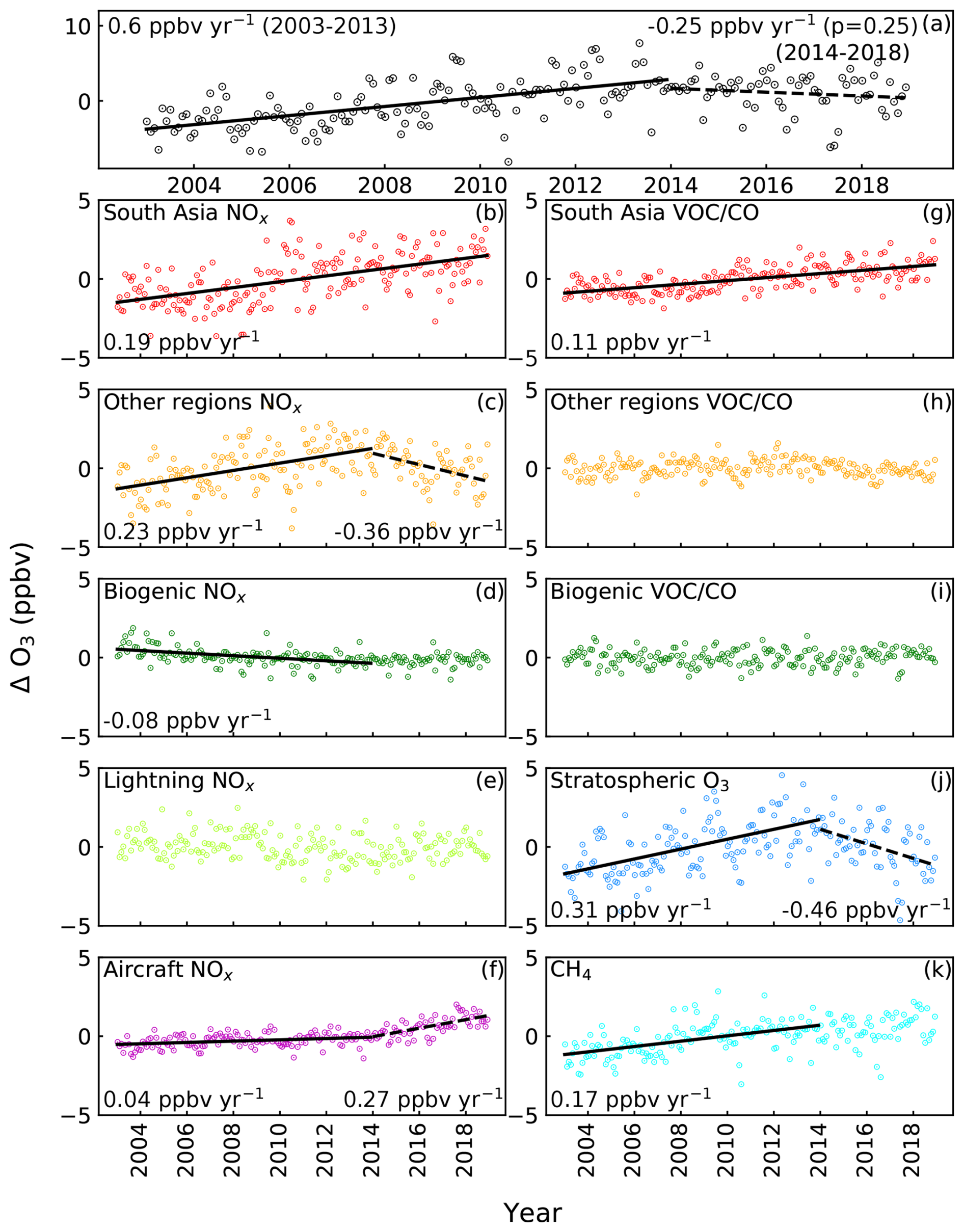
Figure 12Time series of CAM4-Chem simulated de-seasonalised O3 (ΔO3) and contributions from its sources NOx and VOC/CO/CH4 as labelled in each panel during 2003–2018. Black lines show linear regressions and corresponding trend values are shown in respective panels for 2003–2013 (continuous line) and 2014–2018 (dashed line). All trends are statistically significant (p value < 0.01), except for a trend in O3 during 2014–2018 shown in panel (a). Colours of the scatters are chosen the same as in the Fig. 11b and c.
Based on VOC/CO/CH4 tagging (Fig. 11c), largest contribution of 40.1 %–50.3 % (21.9–21.2 ppbv) is from oxidation of CH4, followed by biogenic (11.3 %–19.0 %; 6.2–11.4 ppbv), anthropogenic NMVOC emissions from foreign regions outside South Asia (10.3 %–14.9 %; 6.0–8.1 ppbv), stratospheric intrusion (9.4 %–20.7 %; 5.6–13.8 ppbv). Minor contributors were South Asian anthropogenic NMVOC emissions (4.8 %–9.5 %; 3.1–5.1 ppbv), and biomass burning (2.3 %–4.4 %; 1.6–2.4 ppbv). The contribution of VOC emissions from aircrafts and ships is negligible (< 0.03 ppbv) and the residual is small, 1.4 %–2.5 % (0.8–1.5 ppbv). Contribution from outside South Asia is 10 %–15 % (6–8 ppbv) and further bifurcation of different regional sources (Fig. 11e) shows that East Asia (4 %–5 %; 2–3 ppbv), Middle East (0 %–2 %; 0–1 ppbv), and North America (1 %–2 %; ∼ 1 ppb) have smaller contributions. This suggests that much of the foreign-transported O3 is due to foreign anthropogenic NOx but not due to foreign anthropogenic VOC + CO (Fig. 11d and e). Season-wise contributions from various factors are shown as pie charts in Fig. S10. Among these different sources, the O3 contributions from CH4 oxidation, from biogenic emissions, stratospheric contribution, and from anthropogenic NOx emissions outside South Asia show larger variations (covariance normalised with variance of O3: 0.3–0.6; see coloured text in Fig. 11b and c), and hence these four contributors largely shape the observed seasonal O3 pattern. While stratospheric intrusion in June, 20.7 % (13.8 ppbv), largely drives the peak in O3, biogenic emissions help in maintaining O3 levels during the monsoon season. In other words, global anthropogenic influences plus contributions of natural sources (biogenic + stratospheric intrusion) in conjunction with distinct meteorology of the region sustain substantial O3 even during the monsoon, a quite unique feature in South Asia (Fig. 10a). Since the model shows larger bias during winter, interpretations of source attributions need to be made cautiously.
3.7 Long-term trend in O3 and its precursors
We have analysed CAM4-Chem long-term simulations to know how O3 and its sources have changed over the study region for 1.5 decades, during 2003–2018. Figure 12 shows a time series of de-seasonalised O3 and contributions to O3 from most of the sources as discussed in the previous section. The minor contributors to the study regions (i.e., biomass burning and VOCs from ships) are not shown here. Here, de-seasonalisation is carried out by removing the mean seasonal cycle from monthly average values. Linear regression is shown where the trend is statistically significant (p<0.01). O3 increased over the study region until 2013 with a rate of 0.6 ppbv yr−1 and slightly declined afterwards and the trend is statistically insignificant for the period of 2014–2018 (Fig. 12a). The increasing trend during 2003–2013 is attributed to increasing contributions from NOx from South Asia (0.19 ppbv yr−1) and outside South Asia (0.23 ppbv yr−1), VOC + CO from South Asia (0.11 ppbv yr−1), CH4 (0.17 ppbv yr−1) and stratospheric O3 (0.31 ppbv yr−1). These increasing contributions were partially offset by a small declining contribution from biogenic NOx (−0.08 ppbv yr−1) during 2003–2013. The increase and decrease in NOx contributions from the regions outside South Asia before and after 2013 are due to increasing NOx emission in the Northern Hemisphere until 2013 and decline afterwards (Ansari et al., 2025; Lu et al., 2025). Interestingly, stratospheric O3 also showed a decline during 2014–2018, which is unexpected and needs separate investigations. Thus, slight decline or stationary levels of O3 during 2014–2018 is due to counterbalance between increasing trend in NOx and VOC + CO over South Asia and aircraft NOx emissions; and decreasing trend in NOx emissions outside South Asia and stratospheric contributions.
In view of the significantly higher values of O3, nearing air quality thresholds (Sect. 3.3), we have also analyzed the long-term trend in surface O3 (from CAMS reanalysis) and precursors (from TROPOMI considering region: 77.41–77.70° E; 34.08–34.23° N) during the past few years, as shown in Fig. 13. CAMS O3 shows a positive trend of 0.69 ppbv yr−1 (1.4 % yr−1 with respect to an annual mean level of 50.6 ppbv during 2015). This trend value is larger than previously reported trend over the Indian region at a similar vertical level (0.1 ppbv yr−1 during 1994–2019; Gaudel et al., 2024). The magnitude of the trend over the study region is also higher as compared to the observations of surface O3, 0.1–0.4 ppbv yr−1 (1973–2014) at Thiruvananthapuram (8.5° N; 77.9° E, Nair et al., 2018). Trend at 600 hPa over three locations in India (Thiruvananthapuram, Delhi and Pune) ranged −0.1 to 2.3 % yr−1 during 1989–2001 (Saraf and Beig, 2004). If only June values of CAMS O3 are considered where it closely matches with observations, an increasing trend of 0.74 ppbv yr−1 is found, which is however statistically insignificant during 2015–2024.
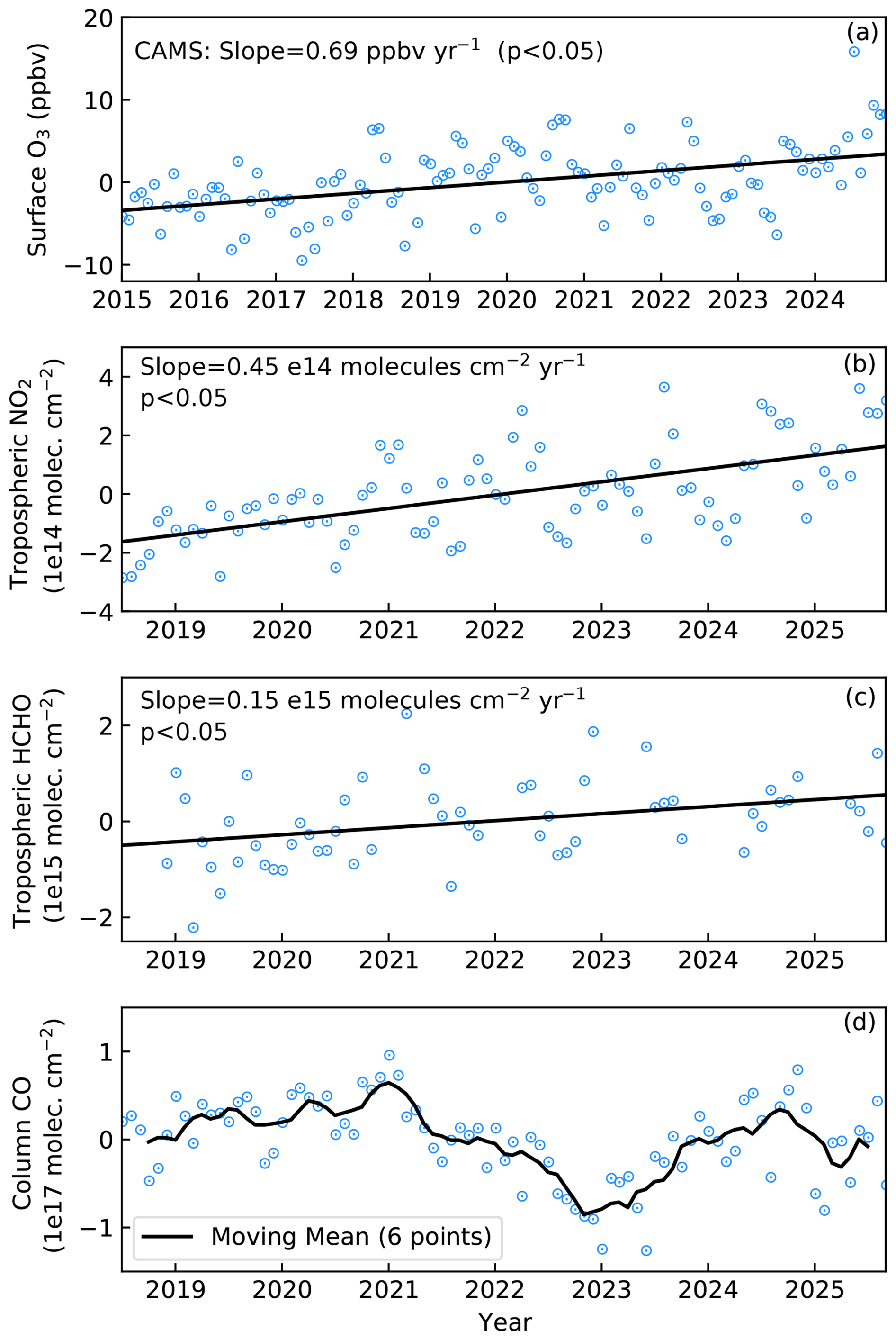
Figure 13Long-term trend in de-seasonalised monthly mean surface O3 from reanalyses (2015–2025) and tropospheric NO2, HCHO and column CO from TROPOMI (2018–2025) over the study region. Trend magnitude, i.e., slope of linear fit, is marked in the top-left corner along with p value.
Satellite-derived NO2 and HCHO, show statistically significant trends of 0.45 × 10¹⁴ (∼ 7 % yr−1 with respect to annual mean 6.44× 10¹⁵ for year 2019) and 0.15 × 10¹⁵ (∼ 4 % yr−1 with respect to annual mean 6.44× 10¹⁵ for year 2019), respectively, during 2018–2025 (Fig. 13b and c). However, since the rate of increase in NO2 is much higher than HCHO, the ratio is declining at the rate of 0.03 per year (Fig. S11), leading to a reduction from 0.65 in 2019 to 0.45 in 2025. This decline is pushing the O3 formation regime towards the VOC-limited regime. If this scenario or trend continues further, local production of O3 is expected to reduce over Leh according to Fig. 8a, however, regional contribution through transport would decide the net increase/decrease scenario. The observed increase in NO2 could be partly attributed to the recent increase in anthropogenic activities including the tourism over the region. Number of tourists in Ladakh have increased over the recent years: 0.28, 0.33, 0.28, 0.52, 0.38, and 0.33 million in 2017, 2018, 2019, 2023, 2024, and 2025, respectively (Dolma, 2020; https://www.ibef.org/states/ladakh-presentation, last access: 16 November 2026; https://lokniwas.ladakh.gov.in/press-details/369, last access: 16 November 2026). Satellite (Resourcesat-2 LISS-IV) based estimation of build-up area over Leh town (77.55–77.63° E; 34.08–34.20° N) shows increase from 1249.9 h (12.5 km2) in 2016 to 1755.3 h (17.5 km2) in 2025 (https://vedas.sac.gov.in/vapps/lama/main.html?app=urban, last access: 16 November 2026; https://vedas.sac.gov.in/vapps/lama/assets/LAMA-interim-report.pdf#page=16, last access: 16 November 2026). Therefore, local anthropogenic emissions would have contributed to the observed increasing trend in precursors (Fig. 13). However, CO does not show consistent increase or decline over the study region (Fig. 13d), and since it has a longer lifetime of a week to 2 months, the regional variation of CO needs to be investigated further.
The dynamics of surface O3 over the Trans-Himalayan region has been comprehensively investigated by combining year-long in situ measurements, analysis of satellite observations, and results from global and regional models. The key findings are summarised as follows.
-
Trans-Himalaya is observed to be a unique environment exhibiting a daytime O3 build-up of 2.6–6.8 ppbv (with rate of 0.6–1.5 ppbv h−1), a feature not observed at high-altitude mountain regions. Despite a daytime build-up partially offsetting the nighttime losses, the region remains a net chemical sink. While photochemistry and vertical entrainment are major drivers of diurnal pattern during winter, advection is an additional contributor during monsoon season.
-
WRF-Chem-derived tendencies suggest that advection is largely responsible for day-to-day changes in O3 during winter, whereas variabilities during monsoon arise from multiple competing processes rather than a single dominant factor.
-
The O3 seasonal cycle peaked in June (65.2 ± 5.8 ppbv) unlike the ubiquitous pre-monsoon peak (April–May) observed over the Himalaya and Gangetic regions. The monsoonal dip (July to September) is much smaller compared to those observed over the Himalaya region. MDA8 is close to and occasionally crosses the WHO threshold of 100 µg m−3 during May–July along with higher values of vegetation-related O3 exposure indices. The photochemistry, fueled by the higher levels of precursors, falling in the NOx-VOC transition regime leads to higher O3 values during May–July.
-
Surface O3 varied from 39–65 ppbv with seasonal amplitude of 26 ppbv, being lower during winter. The CAM4-Chem O3 climatology, after revising stratospheric contribution from CAMS, agrees with the observed seasonal pattern, however, model overestimated wintertime levels by 10–15 ppbv. Nearly half of the O3 in Trans-Himalaya is contributed by anthropogenic NOx emissions from South Asia (15 %–18 %) and outside South Asia (32 %–37 %) throughout the year. From a VOC/CO/CH4 perspective, nearly half of O3 is driven by oxidation of CH4. Among various sources, the following four major contributors largely shape the observed seasonal pattern over the Trans-Himalaya: CH4 oxidation, biogenic emissions of NOx and VOCs, stratospheric O3, and anthropogenic NOx emission from regions outside South Asia. The contribution of NOx emission (17–21 ppbv) is greater than VOC/CO contributions (6–8 ppbv) from the regions outside South Asia. Besides these regional and global photochemical contributions, seasonal peak in O3 is significantly influenced by stratospheric inputs.
-
The study can serve as a reference for designing future field experiments and improvement of global and regional models over the Himalayan region. In particular, measurements of NOx, CH4 and other VOCs, studying the dynamics enhancing O3 in the evening hours, and reducing wintertime biases in the model could be crucial. This study also represents the need for continuation of O3 measurements for air quality monitoring as its levels are close to the threshold.
Overall, the study highlights the varying roles of chemistry, dynamics and regional-to-global anthropogenic sources in controlling the O3 magnitude and variations over the Trans-Himalaya. The rising levels of O3 and its precursors – with surface O3 at 1.4 % yr−1, NO2 at ∼ 7 % yr−1 and HCHO at ∼ 4 % yr−1 – highlight the impact of rapid urbanization and/or tourism, and underscore the need of monitoring of O3 and its precursors along with high-resolution chemistry-transport modeling over this climate-sensitive region of the Trans-Himalaya. Comprehensive measurements of atmospheric composition along with meteorological parameters in this data-sparse region would be crucial for validating satellite-based insights and improving models. This is important as O3 impacts are found substantial in this region although the public health-centric O3 monitoring has been focused mostly in urban and rural areas across India. Observed higher values of O3 are sensitive to NOx as well as VOCs, hence monitoring of various NOx and VOCs besides other precursors is essential for better quantification of the gradient between local emissions and background levels. With new observation-based insights and evaluation of models, future field studies can be designed more strategically and improve the model simulations to further advance the understanding of atmospheric chemistry and dynamics of the Trans-Himalayan region.
In situ measured surface O3 (monthly means) is provided in supplementary (Table S2). Hourly interval O3 (measured and WRF-Chem modelled) and monthly O3 (CAM4-Chem) are available at https://doi.org/10.5281/zenodo.23916482 (Girach et al., 2026).
The supplement related to this article is available online at https://doi.org/10.5194/acp-26-16521-2026-supplement.
IAG and MP conceptualised and designed the study. IAG and SA performed the measurements, with support from AV, LKS, BPS and SS. TA, TB, and NO contributed to the model results and related inputs. IAG led the study and prepared the first draft of the manuscript. All co-authors contributed to the discussions, reviews, and editing.
At least one of the (co-)authors is a member of the editorial board of Atmospheric Chemistry and Physics. The peer-review process was guided by an independent editor, and the authors also have no other competing interests to declare.
Publisher's note: Copernicus Publications remains neutral with regard to jurisdictional claims made in the text, published maps, institutional affiliations, or any other geographical representation in this paper. The authors bear the ultimate responsibility for providing appropriate place names. Views expressed in the text are those of the authors and do not necessarily reflect the views of the publisher.
We gratefully acknowledge Dr. Rashmi Sharma, Deputy Director of EPSA, SAC; Director SAC; Vice-Chancellor of University of Ladakh; and Ladakh Autonomous Hill Development Council for supporting this research activity. We are thankful to India Meteorological Department (IMD) for providing meteorological observations recorded at Leh, Ladakh. We thank Copernicus Atmosphere Monitoring Service (CAMS), ERA-5 reanalysis of the European Center for Medium range Weather Forecasting (ECMWF) for making chemical and meteorological fields from their websites, https://ads.atmosphere.copernicus.eu/datasets/cams-global-reanalysis-eac4?tab=overview (last access: 16 November 2026), and https://cds.climate.copernicus.eu/datasets/reanalysis-era5-pressure-levels?tab=overview (last access: 16 November 2026), respectively. Cloud cover data of INSAT-3DS was obtained from ISRO's MOSDAC website, https://mosdac.gov.in/catalog/satellite (last access: 16 November 2026). We gratefully acknowledge the Sentinel-5p's TROPOMI observations, which were obtained from https://developers.google.com/earth-engine/datasets/catalog/sentinel-5p (last access: 16 November 2026). TA utilized the high-performance computing resources made possible by funding from the Ministry of Science, Research and Culture of the State of Brandenburg (MWFK) and are operated by the IT Services and Operations unit of the Helmholtz Centre Potsdam. TA would like to thank Edward Chan at RIFS for his technical assistance in setting-up the CAM4-Chem model on the GFZ GLIC supercluster. We acknowledge use of the WRF-Chem model preprocessor tools (anthro_emis, mozbc, fire_emiss, etc.) provided by the Atmospheric Chemistry Observations and Modeling Lab of NCAR (National Centre for Atmospheric Research), USA. WRF-Chem simulations were performed on the Param Vikram-1000 High Performance Computing Cluster of the Physical Research Laboratory (PRL), which is a unit of Department of Space, Government of India.
This research has been supported by the LAMA (LAdakh specific Modelling and space Applications) project (https://vedas.sac.gov.in/vapps/lama/, last access: 16 November 2026) under TDP/Adv. R&D programme of Space Applications Centre, Indian Space Research Organisation, Department of Space, Government of India.
This paper was edited by Tanja Schuck and reviewed by two anonymous referees.
Acdan, J. J. M., Pierce, R. B., Dickens, A. F., Adelman, Z., and Nergui, T.: Examining TROPOMI formaldehyde to nitrogen dioxide ratios in the Lake Michigan region: implications for ozone exceedances, Atmos. Chem. Phys., 23, 7867–7885, https://doi.org/10.5194/acp-23-7867-2023, 2023.
Ajayakumar, R. S., Girach, I. A., Soni, M., Ojha, N., and Babu, S. S.: Processes governing the surface ozone over a tropical hill station in the Western Ghats, Atmos. Environ., 319, 120286, https://doi.org/10.1016/j.atmosenv.2023.120286, 2024.
Anagha, K. S. and Kuttippurath, J.: Rising ozone pollution as a threat to wheat yield in India: insights from a concentration-based approach, Environ. Sci. Process. Impacts, 28, 1047–1063, https://doi.org/10.1039/D5EM00850F, 2026.
Ansari, T., Nalam, A., Lupaşcu, A., Hinz, C., Grasse, S., and Butler, T.: Explaining trends and changing seasonal cycles of surface ozone in North America and Europe over the 2000–2018 period: a global modelling study with NOx and VOC tagging, Atmos. Chem. Phys., 25, 16833–16876, https://doi.org/10.5194/acp-25-16833-2025, 2025.
Barth, M. C., Lee, J., Hodzic, A., Pfister, G., Skamarock, W. C., Worden, J., Wong, J., and Noone, D.: Thunderstorms and upper troposphere chemistry during the early stages of the 2006 North American Monsoon, Atmos. Chem. Phys., 12, 11003–11026, https://doi.org/10.5194/acp-12-11003-2012, 2012.
Bhan, S. C., Devrani, A. K., and Sinha, V.: An analysis of monthly rainfall and the meteorological conditions associated with cloudburst over the dry region of Leh (Ladakh), India, MAUSAM, 66, 107–122, https://doi.org/10.54302/mausam.v66i1.371, 2015.
Bhattacharjee, D. and Dutta, R. K.: Mountainous Hazards and Sustainable Livelihood in Leh Valley, in: Indigenous Knowledge and Disaster Risk Reduction, edited by: Panda, G. K., Chatterjee, U., Bandyopadhyay, N., Setiawati, M. D., and Banerjee, D., Springer International Publishing, Cham, 83–105, https://doi.org/10.1007/978-3-031-26143-5_5, 2023.
Borsdorff, T., Aan de Brugh, J., Hu, H., Aben, I., Hasekamp, O., and Landgraf, J.: Measuring Carbon Monoxide With TROPOMI: First Results and a Comparison With ECMWF-IFS Analysis Data, Geophys. Res. Lett., 45, 2826–2832, https://doi.org/10.1002/2018GL077045, 2018.
Butler, T., Lupascu, A., Coates, J., and Zhu, S.: TOAST 1.0: Tropospheric Ozone Attribution of Sources with Tagging for CESM 1.2.2, Geosci. Model Dev., 11, 2825–2840, https://doi.org/10.5194/gmd-11-2825-2018, 2018.
Butler, T., Lupascu, A., and Nalam, A.: Attribution of ground-level ozone to anthropogenic and natural sources of nitrogen oxides and reactive carbon in a global chemical transport model, Atmos. Chem. Phys., 20, 10707–10731, https://doi.org/10.5194/acp-20-10707-2020, 2020.
Carslaw, K. S., Regayre, L. A., Proske, U., Gettelman, A., Sexton, D. M. H., Qian, Y., Marshall, L. R., Wild, O., van Lier-Walqui, M., Oertel, A., Peatier, S., Yang, B., Johnson, J. S., Li, S., McCoy, D. T., Sanderson, B. M., Williamson, C. J., Elsaesser, G. S., Yamazaki, K., and Booth, B. B. B.: Opinion: The importance and future development of perturbed parameter ensembles in climate and atmospheric science, Atmos. Chem. Phys., 26, 4651–4667, https://doi.org/10.5194/acp-26-4651-2026, 2026.
Chevalier, A., Gheusi, F., Delmas, R., Ordóñez, C., Sarrat, C., Zbinden, R., Thouret, V., Athier, G., and Cousin, J.-M.: Influence of altitude on ozone levels and variability in the lower troposphere: a ground-based study for western Europe over the period 2001–2004, Atmos. Chem. Phys., 7, 4311–4326, https://doi.org/10.5194/acp-7-4311-2007, 2007.
Chevuturi, A., Dimri, A. P., and Thayyen, R. J.: Climate change over Leh (Ladakh), India, Theor. Appl. Climatol., 131, 531–545, https://doi.org/10.1007/s00704-016-1989-1, 2018.
Chuwah, C., Van Noije, T., Van Vuuren, D. P., Stehfest, E., and Hazeleger, W.: Global impacts of surface ozone changes on crop yields and land use, Atmos. Environ., 106, 11–23, https://doi.org/10.1016/j.atmosenv.2015.01.062, 2015.
Crippa, M., Guizzardi, D., Oreggioni, G., Muntean, M., and Schaaf, E.: EDGARv5.0 Air Pollutant Emissions, PANGAEA [data set], https://doi.org/10.1594/PANGAEA.921922, 2020.
Crippa, M., Guizzardi, D., Butler, T., Keating, T., Wu, R., Kaminski, J., Kuenen, J., Kurokawa, J., Chatani, S., Morikawa, T., Pouliot, G., Racine, J., Moran, M. D., Klimont, Z., Manseau, P. M., Mashayekhi, R., Henderson, B. H., Smith, S. J., Suchyta, H., Muntean, M., Solazzo, E., Banja, M., Schaaf, E., Pagani, F., Woo, J.-H., Kim, J., Monforti-Ferrario, F., Pisoni, E., Zhang, J., Niemi, D., Sassi, M., Ansari, T., and Foley, K.: The HTAP_v3 emission mosaic: merging regional and global monthly emissions (2000–2018) to support air quality modelling and policies, Earth Syst. Sci. Data, 15, 2667–2694, https://doi.org/10.5194/essd-15-2667-2023, 2023.
Cristofanelli, P., Bracci, A., Sprenger, M., Marinoni, A., Bonafè, U., Calzolari, F., Duchi, R., Laj, P., Pichon, J. M., Roccato, F., Venzac, H., Vuillermoz, E., and Bonasoni, P.: Tropospheric ozone variations at the Nepal Climate Observatory-Pyramid (Himalayas, 5079 ) and influence of deep stratospheric intrusion events, Atmos. Chem. Phys., 10, 6537–6549, https://doi.org/10.5194/acp-10-6537-2010, 2010.
Das, S., Giorgi, F., Coppola, E., Panicker, A. S., Gautam, A. S., Nair, V. S., and Giuliani, G.: Linkage between the absorbing aerosol-induced snow darkening effects over the Himalayas-Tibetan Plateau and the pre-monsoon climate over northern India, Theor. Appl. Climatol., 147, 1033–1048, https://doi.org/10.1007/s00704-021-03871-y, 2022.
De Smedt, I., Theys, N., Yu, H., Danckaert, T., Lerot, C., Compernolle, S., Van Roozendael, M., Richter, A., Hilboll, A., Peters, E., Pedergnana, M., Loyola, D., Beirle, S., Wagner, T., Eskes, H., van Geffen, J., Boersma, K. F., and Veefkind, P.: Algorithm theoretical baseline for formaldehyde retrievals from S5P TROPOMI and from the QA4ECV project, Atmos. Meas. Tech., 11, 2395–2426, https://doi.org/10.5194/amt-11-2395-2018, 2018.
De Smedt, I., Pinardi, G., Vigouroux, C., Compernolle, S., Bais, A., Benavent, N., Boersma, F., Chan, K.-L., Donner, S., Eichmann, K.-U., Hedelt, P., Hendrick, F., Irie, H., Kumar, V., Lambert, J.-C., Langerock, B., Lerot, C., Liu, C., Loyola, D., Piters, A., Richter, A., Rivera Cárdenas, C., Romahn, F., Ryan, R. G., Sinha, V., Theys, N., Vlietinck, J., Wagner, T., Wang, T., Yu, H., and Van Roozendael, M.: Comparative assessment of TROPOMI and OMI formaldehyde observations and validation against MAX-DOAS network column measurements, Atmos. Chem. Phys., 21, 12561–12593, https://doi.org/10.5194/acp-21-12561-2021, 2021.
Dolma, Y.: Tourism in Ladakh: Trends and composition, International Journal of Research in Social Sciences, 10, 127–140, https://www.ijmra.us/2020ijrss_december.php (last access: 16 November 2026), 2020.
Dubey, J., Singh, D. S., and Sati, S. P.: Cryosphere Response to Climate Change and Disaster Risk Reduction in the Arid Northwestern Ladakh Himalaya, in: Ecosystem-based Approaches for Resilience Building in Himalayan Landscapes, edited by: Khan, Y. D. I., Goswami, M., and Nautiyal, S., Springer Nature Singapore, Singapore, 3–27, https://doi.org/10.1007/978-981-95-2007-7_1, 2025.
Emmerichs, T., Kerkweg, A., Ouwersloot, H., Fares, S., Mammarella, I., and Taraborrelli, D.: A revised dry deposition scheme for land–atmosphere exchange of trace gases in ECHAM/MESSy v2.54, Geosci. Model Dev., 14, 495–519, https://doi.org/10.5194/gmd-14-495-2021, 2021.
Emmons, L. K., Walters, S., Hess, P. G., Lamarque, J.-F., Pfister, G. G., Fillmore, D., Granier, C., Guenther, A., Kinnison, D., Laepple, T., Orlando, J., Tie, X., Tyndall, G., Wiedinmyer, C., Baughcum, S. L., and Kloster, S.: Description and evaluation of the Model for Ozone and Related chemical Tracers, version 4 (MOZART-4), Geosci. Model Dev., 3, 43–67, https://doi.org/10.5194/gmd-3-43-2010, 2010.
Fuhrer, J., Skärby, L., and Ashmore, M. R.: Critical levels for ozone effects on vegetation in Europe, Environ. Pollut., 97, 91–106, https://doi.org/10.1016/S0269-7491(97)00067-5, 1997.
Gao, Y., Kou, W., Cheng, W., Guo, X., Qu, B., Wu, Y., Zhang, S., Liao, H., Chen, D., Leung, L. R., Wild, O., Zhang, J., Lin, G., Su, H., Cheng, Y., Pöschl, U., Pozzer, A., Zhang, L., Lamarque, J., Guenther, A. B., Brasseur, G., Liu, Z., Lu, H., Li, C., Zhao, B., Wang, S., Huang, X., Pan, J., Liu, G., Liu, X., Lin, H., Zhao, Y., Zhao, C., Meng, J., Yao, X., Gao, H., and Wu, L.: Reducing Long-Standing Surface Ozone Overestimation in Earth System Modeling by High-Resolution Simulation and Dry Deposition Improvement, J. Adv. Model. Earth Sy., 17, e2023MS004192, https://doi.org/10.1029/2023MS004192, 2025.
Gaudel, A., Bourgeois, I., Li, M., Chang, K.-L., Ziemke, J., Sauvage, B., Stauffer, R. M., Thompson, A. M., Kollonige, D. E., Smith, N., Hubert, D., Keppens, A., Cuesta, J., Heue, K.-P., Veefkind, P., Aikin, K., Peischl, J., Thompson, C. R., Ryerson, T. B., Frost, G. J., McDonald, B. C., and Cooper, O. R.: Tropical tropospheric ozone distribution and trends from in situ and satellite data, Atmos. Chem. Phys., 24, 9975–10000, https://doi.org/10.5194/acp-24-9975-2024, 2024.
GBD 2019 Risk Factors Collaborators: Global burden of 87 risk factors in 204 countries and territories, 1990–2019: a systematic analysis for the Global Burden of Disease Study 2019, Lancet, 396, 1223–1249, https://doi.org/10.1016/S0140-6736(20)30752-2, 2020.
Gettelman, A., Mills, M. J., Kinnison, D. E., Garcia, R. R., Smith, A. K., Marsh, D. R., Tilmes, S., Vitt, F., Bardeen, C. G., McInerny, J., Liu, H. -L., Solomon, S. C., Polvani, L. M., Emmons, L. K., Lamarque, J. -F., Richter, J. H., Glanville, A. S., Bacmeister, J. T., Phillips, A. S., Neale, R. B., Simpson, I. R., DuVivier, A. K., Hodzic, A., and Randel, W. J.: The Whole Atmosphere Community Climate Model Version 6 (WACCM6), J. Geophys. Res.-Atmos., 124, 12380–12403, https://doi.org/10.1029/2019JD030943, 2019.
Ghude, S. D., Kalita, G., Jat, R., Govardhan, G., Debnath, S., Yadav, P. P., Ambulkar, R., Kumar, R., and Attri, S. D.: The role of atmospheric feedback and groundwater conservation policies in degrading air quality in Delhi, npj Clean Air, 1, 12, https://doi.org/10.1038/s44407-025-00012-x, 2025.
Girach, I. A., Ojha, N., Nair, P. R., Pozzer, A., Tiwari, Y. K., Kumar, K. R., and Lelieveld, J.: Variations in O3, CO, and CH4 over the Bay of Bengal during the summer monsoon season: shipborne measurements and model simulations, Atmos. Chem. Phys., 17, 257–275, https://doi.org/10.5194/acp-17-257-2017, 2017.
Girach, I., Ojha, N., and Ansari, T.: Surface ozone over the Trans-Himalaya (In situ, WRF-Chem, and CAM4-Chem), Zenodo [data set], https://doi.org/10.5281/zenodo.23916482, 2026.
Goodrich, C. G., Udas, P. B., and Larrington-Spencer, H.: Conceptualizing gendered vulnerability to climate change in the Hindu Kush Himalaya: Contextual conditions and drivers of change, Environ. Dev., 31, 9–18, https://doi.org/10.1016/j.envdev.2018.11.003, 2019.
Grell, G. A. and Dévényi, D.: A generalized approach to parameterizing convection combining ensemble and data assimilation techniques, Geophys. Res. Lett., 29, https://doi.org/10.1029/2002GL015311, 2002.
Grell, G. A., Peckham, S. E., Schmitz, R., McKeen, S. A., Frost, G., Skamarock, W. C., and Eder, B.: Fully coupled “online” chemistry within the WRF model, Atmos. Environ., 39, 6957–6975, https://doi.org/10.1016/j.atmosenv.2005.04.027, 2005.
Guenther, A., Karl, T., Harley, P., Wiedinmyer, C., Palmer, P. I., and Geron, C.: Estimates of global terrestrial isoprene emissions using MEGAN (Model of Emissions of Gases and Aerosols from Nature), Atmos. Chem. Phys., 6, 3181–3210, https://doi.org/10.5194/acp-6-3181-2006, 2006.
Harithasree, S., Sharma, K., Girach, I. A., Sahu, L. K., Nair, P. R., Singh, N., Flemming, J., Babu, S. S., and Ojha, N.: Surface ozone over Doon valley of the Indian Himalaya: Characteristics, impact assessment, and model results, Atmospheric Environment X, 21, 100247, https://doi.org/10.1016/j.aeaoa.2024.100247, 2024.
Hassan, M. A., Mehmood, T., Liu, J., Luo, X., Li, X., Tanveer, M., Faheem, M., Shakoor, A., Dar, A. A., and Abid, M.: A review of particulate pollution over Himalaya region: Characteristics and salient factors contributing ambient PM pollution, Atmos. Environ., 294, 119472, https://doi.org/10.1016/j.atmosenv.2022.119472, 2023.
Hersbach, H., Bell, B., Berrisford, P., Hirahara, S., Horányi, A., Muñoz-Sabater, J., Nicolas, J., Peubey, C., Radu, R., Schepers, D., Simmons, A., Soci, C., Abdalla, S., Abellan, X., Balsamo, G., Bechtold, P., Biavati, G., Bidlot, J., Bonavita, M., De Chiara, G., Dahlgren, P., Dee, D., Diamantakis, M., Dragani, R., Flemming, J., Forbes, R., Fuentes, M., Geer, A., Haimberger, L., Healy, S., Hogan, R. J., Hólm, E., Janisková, M., Keeley, S., Laloyaux, P., Lopez, P., Lupu, C., Radnoti, G., De Rosnay, P., Rozum, I., Vamborg, F., Villaume, S., and Thépaut, J.: The ERA5 global reanalysis, Q. J. Roy. Meteor. Soc., 146, 1999–2049, https://doi.org/10.1002/qj.3803, 2020.
Hogsett, W. E., Tingey, D. T., and Lee, E. H.: Ozone Exposure Indices: Concepts for Development and Evaluation of their Use, in: Assessment of Crop Loss From Air Pollutants, edited by: Heck, W. W., Taylor, O. C., and Tingey, D. T., Springer Netherlands, Dordrecht, 107–138, https://doi.org/10.1007/978-94-009-1367-7_7, 1988.
Hong, S.-Y., Noh, Y., and Dudhia, J.: A New Vertical Diffusion Package with an Explicit Treatment of Entrainment Processes, Mon. Weather Rev., 134, 2318–2341, https://doi.org/10.1175/MWR3199.1, 2006.
Huijnen, V., Williams, J., van Weele, M., van Noije, T., Krol, M., Dentener, F., Segers, A., Houweling, S., Peters, W., de Laat, J., Boersma, F., Bergamaschi, P., van Velthoven, P., Le Sager, P., Eskes, H., Alkemade, F., Scheele, R., Nédélec, P., and Pätz, H.-W.: The global chemistry transport model TM5: description and evaluation of the tropospheric chemistry version 3.0, Geosci. Model Dev., 3, 445–473, https://doi.org/10.5194/gmd-3-445-2010, 2010.
Inness, A., Ades, M., Agustí-Panareda, A., Barré, J., Benedictow, A., Blechschmidt, A.-M., Dominguez, J. J., Engelen, R., Eskes, H., Flemming, J., Huijnen, V., Jones, L., Kipling, Z., Massart, S., Parrington, M., Peuch, V.-H., Razinger, M., Remy, S., Schulz, M., and Suttie, M.: The CAMS reanalysis of atmospheric composition, Atmos. Chem. Phys., 19, 3515–3556, https://doi.org/10.5194/acp-19-3515-2019, 2019.
Jiao, G., Chen, L., Li, K., Zhu, J., Dong, X., Zhu, X., Yang, Y., Yue, X., and Liao, H.: Worsened Ozone Pollution Exacerbates the Loss of Agricultural Production in China, J. Geophys. Res.-Atmos., 130, e2024JD042781, https://doi.org/10.1029/2024JD042781, 2025.
Jin, X., Fiore, A. M., Murray, L. T., Valin, L. C., Lamsal, L. N., Duncan, B., Folkert Boersma, K., De Smedt, I., Abad, G. G., Chance, K., and Tonnesen, G. S.: Evaluating a Space-Based Indicator of Surface Ozone-NOx-VOC Sensitivity Over Midlatitude Source Regions and Application to Decadal Trends, J. Geophys. Res.-Atmos., 122, https://doi.org/10.1002/2017JD026720, 2017.
Kaylor, S. D., Snell Taylor, S. J., and Herrick, J. D.: Estimates of biomass reductions of ozone sensitive herbaceous plants in California, Sci. Total Environ., 878, 163134, https://doi.org/10.1016/j.scitotenv.2023.163134, 2023.
Khanday, A. A., Rather, G. M., Kumar, M. A., and Lone, A. H.: Environmental Sustainability and Its Impact on Public Health in Ladakh-India, in: Sustainability and Health Informatics, edited by: Tripathi, G., Shakya, A., Kanga, S., Guite, L. T. S., and Singh, S. K., Springer Nature Singapore, Singapore, 183–198, https://doi.org/10.1007/978-981-97-6706-9_9, 2024.
Kumar, R., Naja, M., Venkataramani, S., and Wild, O.: Variations in surface ozone at Nainital: A high-altitude site in the central Himalayas, J. Geophys. Res.-Atmos., 115, 2009JD013715, https://doi.org/10.1029/2009JD013715, 2010.
Kumar, R., Naja, M., Pfister, G. G., Barth, M. C., and Brasseur, G. P.: Simulations over South Asia using the Weather Research and Forecasting model with Chemistry (WRF-Chem): set-up and meteorological evaluation, Geosci. Model Dev., 5, 321–343, https://doi.org/10.5194/gmd-5-321-2012, 2012a.
Kumar, R., Naja, M., Pfister, G. G., Barth, M. C., Wiedinmyer, C., and Brasseur, G. P.: Simulations over South Asia using the Weather Research and Forecasting model with Chemistry (WRF-Chem): chemistry evaluation and initial results, Geosci. Model Dev., 5, 619–648, https://doi.org/10.5194/gmd-5-619-2012, 2012b.
Lal, S., Peshin, S. K., Naja, M., and Venkataramani, S.: Variability of Ozone and Related Trace Gases Over India, in: Observed Climate Variability and Change over the Indian Region, edited by: Rajeevan, M. N. and Nayak, S., Springer Singapore, Singapore, 249–269, https://doi.org/10.1007/978-981-10-2531-0_14, 2017.
Landgraf, J., aan de Brugh, J., Scheepmaker, R., Borsdorff, T., Hu, H., Houweling, S., Butz, A., Aben, I., and Hasekamp, O.: Carbon monoxide total column retrievals from TROPOMI shortwave infrared measurements, Atmos. Meas. Tech., 9, 4955–4975, https://doi.org/10.5194/amt-9-4955-2016, 2016.
Lee, E. H., Tingey, D. T., and Hogsett, W. E.: Evaluation of ozone exposure indices in exposure-response modeling, Environ. Pollut., 53, 43–62, https://doi.org/10.1016/0269-7491(88)90024-3, 1988.
Lee, J., Han, J., Park, J., Ahn, J.-Y., and Lee, G.: Long-term changes of rice yield loss estimated with AOT40 and M7 metrics using comprehensive ozone and rice cultivation data over South Korea, Asian J. Atmospheric Environ., 17, 21, https://doi.org/10.1007/s44273-023-00021-w, 2023.
Lefohn, A. S. and Runeckles, V. C.: Establishing standards to protect vegetation–ozone exposure/dose considerations, Atmos. Environ. 1967, 21, 561–568, https://doi.org/10.1016/0004-6981(87)90038-2, 1987.
Liao, Z., Zhang, J., Gao, M., and Ma, Z.: Widespread stratospheric intrusion influence on summer ozone pollution over China revealed by multi-site ozonesonde and validated EAC4 reanalysis, Atmos. Chem. Phys., 25, 14865–14877, https://doi.org/10.5194/acp-25-14865-2025, 2025.
Liu, Z., Doherty, R. M., Wild, O., O'Connor, F. M., and Turnock, S. T.: Correcting ozone biases in a global chemistry–climate model: implications for future ozone, Atmos. Chem. Phys., 22, 12543–12557, https://doi.org/10.5194/acp-22-12543-2022, 2022.
Lu, X., Liu, Y., Su, J., Weng, X., Ansari, T., Zhang, Y., He, G., Zhu, Y., Wang, H., Zeng, G., Li, J., He, C., Li, S., Amnuaylojaroen, T., Butler, T., Fan, Q., Fan, S., Forster, G. L., Gao, M., Hu, J., Kanaya, Y., Latif, M. T., Lu, K., Nédélec, P., Nowack, P., Sauvage, B., Xu, X., Zhang, L., Li, K., Koo, J.-H., and Nagashima, T.: Tropospheric ozone trends and attributions over East and Southeast Asia in 1995–2019: an integrated assessment using statistical methods, machine learning models, and multiple chemical transport models, Atmos. Chem. Phys., 25, 7991–8028, https://doi.org/10.5194/acp-25-7991-2025, 2025.
Mahata, K. S., Rupakheti, M., Panday, A. K., Bhardwaj, P., Naja, M., Singh, A., Mues, A., Cristofanelli, P., Pudasainee, D., Bonasoni, P., and Lawrence, M. G.: Observation and analysis of spatiotemporal characteristics of surface ozone and carbon monoxide at multiple sites in the Kathmandu Valley, Nepal, Atmos. Chem. Phys., 18, 14113–14132, https://doi.org/10.5194/acp-18-14113-2018, 2018.
Martin, R. V., Fiore, A. M., and Van Donkelaar, A.: Space-based diagnosis of surface ozone sensitivity to anthropogenic emissions, Geophys. Res. Lett., 31, 2004GL019416, https://doi.org/10.1029/2004GL019416, 2004.
Mills, G., Buse, A., Gimeno, B., Bermejo, V., Holland, M., Emberson, L., and Pleijel, H.: A synthesis of AOT40-based response functions and critical levels of ozone for agricultural and horticultural crops, Atmos. Environ., 41, 2630–2643, https://doi.org/10.1016/j.atmosenv.2006.11.016, 2007.
Miyazaki, K., Marchetti, Y., Montgomery, J., Lu, S., and Bowman, K.: Identifying drivers of surface ozone bias in global chemical reanalysis with explainable machine learning, Atmos. Chem. Phys., 25, 8507–8532, https://doi.org/10.5194/acp-25-8507-2025, 2025.
Mogno, C. and Marvin, M. R.: EDGAR v5.0 emissions inventory speciated for the MOZART chemical mechanism (v1.0.0), Zenodo [data set], https://doi.org/10.5281/zenodo.6130621, 2022.
Nair, P. R., Ajayakumar, R. S., David, L. M., Girach, I. A., and Mottungan, K.: Decadal changes in surface ozone at the tropical station Thiruvananthapuram (8.542° N, 76.858° E), India: effects of anthropogenic activities and meteorological variability, Environ. Sci. Pollut. Res., 25, 14827–14843, https://doi.org/10.1007/s11356-018-1695-x, 2018.
Nair, V. S., Usha, K. H., and Babu, S. S.: Elevation-dependence of warming due to aerosol-induced snow darkening over the Himalayan-Tibetan region, Environ. Res. Lett., 19, 014049, https://doi.org/10.1088/1748-9326/ad1346, 2024.
Naja, M.: Diurnal and seasonal variabilities in surface ozone at a high altitude site Mt Abu (24.6° N, 72.7° E, 1680 m asl) in India, Atmos. Environ., 37, 4205–4215, https://doi.org/10.1016/S1352-2310(03)00565-X, 2003.
Nalam, A., Lupaşcu, A., Ansari, T., and Butler, T.: Regional and sectoral contributions of NOx and reactive carbon emission sources to global trends in tropospheric ozone during the 2000–2018 period, Atmos. Chem. Phys., 25, 5287–5311, https://doi.org/10.5194/acp-25-5287-2025, 2025.
Ningombam, S. S., Bagare, S. P., Srivastava, A. K., Kanawade, V. P., Singh, R. B., and Padhy, S. K.: Temporal asymmetry in aerosol optical characteristics: A case study at a high-altitude station, Hanle, in Ladakh region, J. Atmos. Sol.-Terr. Phy., 121, 123–131, https://doi.org/10.1016/j.jastp.2014.10.012, 2014.
Ojha, N., Naja, M., Singh, K. P., Sarangi, T., Kumar, R., Lal, S., Lawrence, M. G., Butler, T. M., and Chandola, H. C.: Variabilities in ozone at a semi-urban site in the Indo-Gangetic Plain region: Association with the meteorology and regional processes, J. Geophys. Res.-Atmos., 117, 2012JD017716, https://doi.org/10.1029/2012JD017716, 2012.
Ojha, N., Girach, I., Sharma, K., Nair, P., Singh, J., Sharma, N., Singh, N., Flemming, J., Inness, A., and Subrahmanyam, K. V.: Surface ozone in the Doon Valley of the Himalayan foothills during spring, Environ. Sci. Pollut. Res., 26, 19155–19170, https://doi.org/10.1007/s11356-019-05085-2, 2019.
Ojha, N., Girach, I., Soni, M., and Singh, N.: Distribution of reactive trace gases over South Asia: Observations and modeling, in: Asian Atmospheric Pollution, edited by: Singh, R. P., Elsevier, 147–169, https://doi.org/10.1016/B978-0-12-816693-2.00022-6, 2022.
Okamoto, S. and Tanimoto, H.: A review of atmospheric chemistry observations at mountain sites, Prog. Earth Planet. Sci., 3, 34, https://doi.org/10.1186/s40645-016-0109-2, 2016.
Otte, T. L.: The Impact of Nudging in the Meteorological Model for Retrospective Air Quality Simulations. Part I: Evaluation against National Observation Networks, J. Appl. Meteorol. Clim., 47, 1853–1867, https://doi.org/10.1175/2007JAMC1790.1, 2008.
Pandit, M. K.: The Himalayas must be protected, Nature, 501, 283–283, https://doi.org/10.1038/501283a, 2013.
Park, S., Son, S.-W., Jung, M.-I., Park, J., and Park, S. S.: Evaluation of tropospheric ozone reanalyses with independent ozonesonde observations in East Asia, Geosci. Lett., 7, 12, https://doi.org/10.1186/s40562-020-00161-9, 2020.
Pasternak, A., Müller, J.-F., Poraicu, C., Merlaud, A., Tack, F., and Stavrakou, T.: Validation of TROPOMI and WRF-Chem NO2 across seasons using SWING+ and surface observations over Bucharest, Atmos. Chem. Phys., 26, 5185–5212, https://doi.org/10.5194/acp-26-5185-2026, 2026.
Prather, M. J. and Zhu, X.: Lifetimes and timescales of tropospheric ozone, Elementa Sci. Anth., 12, 00112, https://doi.org/10.1525/elementa.2023.00112, 2024.
Putero, D., Cristofanelli, P., Marinoni, A., Adhikary, B., Duchi, R., Shrestha, S. D., Verza, G. P., Landi, T. C., Calzolari, F., Busetto, M., Agrillo, G., Biancofiore, F., Di Carlo, P., Panday, A. K., Rupakheti, M., and Bonasoni, P.: Seasonal variation of ozone and black carbon observed at Paknajol, an urban site in the Kathmandu Valley, Nepal, Atmos. Chem. Phys., 15, 13957–13971, https://doi.org/10.5194/acp-15-13957-2015, 2015.
Ren, J., Guo, F., and Xie, S.: Diagnosing ozone–NOx–VOC sensitivity and revealing causes of ozone increases in China based on 2013–2021 satellite retrievals, Atmos. Chem. Phys., 22, 15035–15047, https://doi.org/10.5194/acp-22-15035-2022, 2022.
Romatschke, U. and Houze, R. A.: Characteristics of Precipitating Convective Systems in the South Asian Monsoon, J. Hydrometeorol., 12, 3–26, https://doi.org/10.1175/2010JHM1289.1, 2011.
Sahu, L. K., Lal, S., Thouret, V., and Smit, H. G.: Seasonality of tropospheric ozone and water vapor over Delhi, India: a study based on MOZAIC measurement data, J. Atmos. Chem., 62, 151–174, https://doi.org/10.1007/s10874-010-9146-1, 2009.
Santra, P.: Scope of Solar Energy in Cold Arid Region of India at Leh Ladakh, Ann. Arid Zone, 54, https://doi.org/10.56093/aaz.v54i3-4.63046, 2016.
Saraf, N. and Beig, G.: Long-term trends in tropospheric ozone over the Indian tropical region, Geophys. Res. Lett., 31, 2003GL018516, https://doi.org/10.1029/2003GL018516, 2004.
Sarangi, T., Naja, M., Ojha, N., Kumar, R., Lal, S., Venkataramani, S., Kumar, A., Sagar, R., and Chandola, H. C.: First simultaneous measurements of ozone, CO, and NOy at a high-altitude regional representative site in the central Himalayas, J. Geophys. Res.-Atmos., 119, 1592–1611, https://doi.org/10.1002/2013JD020631, 2014.
Seinfeld, J. H. and Pandis, S. N.: Atmospheric Chemistry and Physics: From Air Pollution to Climate Change, Wiley, USA, ISBN 978-1-118-94740-1, 2016.
Sharma, A., Ojha, N., Pozzer, A., Mar, K. A., Beig, G., Lelieveld, J., and Gunthe, S. S.: WRF-Chem simulated surface ozone over south Asia during the pre-monsoon: effects of emission inventories and chemical mechanisms, Atmos. Chem. Phys., 17, 14393–14413, https://doi.org/10.5194/acp-17-14393-2017, 2017.
Sharma, P., Kuniyal, J. C., Chand, K., Guleria, R. P., Dhyani, P. P., and Chauhan, C.: Surface ozone concentration and its behaviour with aerosols in the northwestern Himalaya, India, Atmos. Environ., 71, 44–53, https://doi.org/10.1016/j.atmosenv.2012.12.042, 2013.
Sindelarova, K., Markova, J., Simpson, D., Huszar, P., Karlicky, J., Darras, S., and Granier, C.: High-resolution biogenic global emission inventory for the time period 2000–2019 for air quality modelling, Earth Syst. Sci. Data, 14, 251–270, https://doi.org/10.5194/essd-14-251-2022, 2022.
Singh, J., Singh, N., Ojha, N., Sharma, A., Pozzer, A., Kiran Kumar, N., Rajeev, K., Gunthe, S. S., and Kotamarthi, V. R.: Effects of spatial resolution on WRF v3.8.1 simulated meteorology over the central Himalaya, Geosci. Model Dev., 14, 1427–1443, https://doi.org/10.5194/gmd-14-1427-2021, 2021.
Sinha, P. R., Sahu, L. K., Manchanda, R. K., Sheel, V., Deushi, M., Kajino, M., Schultz, M. G., Nagendra, N., Kumar, P., Trivedi, D. B., Koli, S. K., Peshin, S. K., Swamy, Y. V., Tzanis, C. G., and Sreenivasan, S.: Transport of tropospheric and stratospheric ozone over India: Balloon-borne observations and modeling analysis, Atmos. Environ., 131, 228–242, https://doi.org/10.1016/j.atmosenv.2016.02.001, 2016.
Skamarock, W. C., Klemp, J. B., Dudhia, J., Gill, D. O., Liu, Z., Berner, J., Wang, W., Powers, J. G., Duda, M. G., Barker, D. M., and Huang, X.-Y.: A Description of the Advanced Research WRF Model Version 4, NSF National Center for Atmospheric Research, https://doi.org/10.5065/1DFH-6P97, 2019.
Škerlak, B., Sprenger, M., and Wernli, H.: A global climatology of stratosphere–troposphere exchange using the ERA-Interim data set from 1979 to 2011, Atmos. Chem. Phys., 14, 913–937, https://doi.org/10.5194/acp-14-913-2014, 2014.
Souri, A. H., Johnson, M. S., Wolfe, G. M., Crawford, J. H., Fried, A., Wisthaler, A., Brune, W. H., Blake, D. R., Weinheimer, A. J., Verhoelst, T., Compernolle, S., Pinardi, G., Vigouroux, C., Langerock, B., Choi, S., Lamsal, L., Zhu, L., Sun, S., Cohen, R. C., Min, K.-E., Cho, C., Philip, S., Liu, X., and Chance, K.: Characterization of errors in satellite-based tropospheric column ratios with respect to chemistry, column-to-PBL translation, spatial representation, and retrieval uncertainties, Atmos. Chem. Phys., 23, 1963–1986, https://doi.org/10.5194/acp-23-1963-2023, 2023.
Tanimoto, H., Mukai, H., Sawa, Y., Matsueda, H., Yonemura, S., Wang, T., Poon, S., Wong, A., Lee, G., Jung, J. Y., Kim, K. R., Lee, M. H., Lin, N. H., Wang, J. L., Ou-Yang, C. F., Wu, C. F., Akimoto, H., Pochanart, P., Tsuboi, K., Doi, H., Zellweger, C., and Klausen, J.: Direct assessment of international consistency of standards for ground-level ozone: strategy and implementation toward metrological traceability network in Asia, J. Environ. Monit., 9, 1183, https://doi.org/10.1039/b701230f, 2007.
Tilmes, S., Lamarque, J.-F., Emmons, L. K., Kinnison, D. E., Ma, P.-L., Liu, X., Ghan, S., Bardeen, C., Arnold, S., Deeter, M., Vitt, F., Ryerson, T., Elkins, J. W., Moore, F., Spackman, J. R., and Val Martin, M.: Description and evaluation of tropospheric chemistry and aerosols in the Community Earth System Model (CESM1.2), Geosci. Model Dev., 8, 1395–1426, https://doi.org/10.5194/gmd-8-1395-2015, 2015.
Tsutsumi, Y., Zaizen, Y., and Makino, Y.: Tropospheric ozone measurement at the top of Mt. Fuji, Geophys. Res. Lett., 21, 1727–1730, https://doi.org/10.1029/94GL01107, 1994.
Turnock, S. T., Akritidis, D., Horowitz, L., Mertens, M., Pozzer, A., Reddington, C. L., Wang, H., Zhou, P., and O'Connor, F.: Drivers of change in peak-season surface ozone concentrations and impacts on human health over the historical period (1850–2014), Atmos. Chem. Phys., 25, 7111–7136, https://doi.org/10.5194/acp-25-7111-2025, 2025.
Udayasoorian, C., Jayabalakrishnan, R. M., Suguna, A. R., Venkataramani, S., and Lal, S.: Diurnal and seasonal characteristics of ozone and NOx over a high-altitude western Ghats location in southern India, Advances in Applied Science Research, 4, 309–320, https://www.primescholars.com/abstract/diurnal-and-seasonal-characteristics-of-ozone-and-nox-over-a-high-altitudewestern-ghats-location-in-southern-india-89717.html (last access: 16 November 2026), 2013.
US EPA: Integrated Science Assessment (ISA) for Ozone and Related Photochemical Oxidants, https://assessments.epa.gov/isa/document/&deid%3D247492 (last access: 16 November 2026), 2013.
van der Werf, G. R., Randerson, J. T., Giglio, L., Collatz, G. J., Mu, M., Kasibhatla, P. S., Morton, D. C., DeFries, R. S., Jin, Y., and van Leeuwen, T. T.: Global fire emissions and the contribution of deforestation, savanna, forest, agricultural, and peat fires (1997–2009), Atmos. Chem. Phys., 10, 11707–11735, https://doi.org/10.5194/acp-10-11707-2010, 2010.
van Geffen, J., Eskes, H., Compernolle, S., Pinardi, G., Verhoelst, T., Lambert, J.-C., Sneep, M., ter Linden, M., Ludewig, A., Boersma, K. F., and Veefkind, J. P.: Sentinel-5P TROPOMI NO2 retrieval: impact of version v2.2 improvements and comparisons with OMI and ground-based data, Atmos. Meas. Tech., 15, 2037–2060, https://doi.org/10.5194/amt-15-2037-2022, 2022.
Wester, P., Mishra, A., Mukherji, A., and Shrestha, A. B. (Eds.): The Hindu Kush Himalaya Assessment: Mountains, Climate Change, Sustainability and People, Springer International Publishing, Cham, https://doi.org/10.1007/978-3-319-92288-1, 2019.
WHO: WHO global air quality guidelines: particulate matter (PM2.5 and PM10), ozone, nitrogen dioxide, sulfur dioxide and carbon monoxide, World Health Organization, https://www.who.int/publications/i/item/9789240034228 (last access: 16 November 2026), 2021.
Wiedinmyer, C., Kimura, Y., McDonald-Buller, E. C., Emmons, L. K., Buchholz, R. R., Tang, W., Seto, K., Joseph, M. B., Barsanti, K. C., Carlton, A. G., and Yokelson, R.: The Fire Inventory from NCAR version 2.5: an updated global fire emissions model for climate and chemistry applications, Geosci. Model Dev., 16, 3873–3891, https://doi.org/10.5194/gmd-16-3873-2023, 2023.
Wild, O. and Ryan, E. M.: Quantifying and addressing the uncertainties in tropospheric ozone and OH in a global chemistry transport model, Atmos. Chem. Phys., 26, 2255–2273, https://doi.org/10.5194/acp-26-2255-2026, 2026.
Yamartino, R. J.: A Comparison of Several “Single-Pass” Estimators of the Standard Deviation of Wind Direction, J. Clim. Appl. Meteorol., 23, 1362–1366, https://doi.org/10.1175/1520-0450(1984)023<1362:ACOSPE>2.0.CO;2, 1984.
Yongde, K. and Xinchun, L.: Characteristics and potential source areas of ozone pollution in Pamir Plateau, Sci. Total Environ., 967, 178783, https://doi.org/10.1016/j.scitotenv.2025.178783, 2025.
Zaveri, R. A., Easter, R. C., Fast, J. D., and Peters, L. K.: Model for Simulating Aerosol Interactions and Chemistry (MOSAIC), J. Geophys. Res.-Atmos., 113, 2007JD008782, https://doi.org/10.1029/2007JD008782, 2008.
Ziegler, A. D., Cantarero, S. I., Wasson, R. J., Srivastava, P., Spalzin, S., Chow, W. T. L., and Gillen, J.: A clear and present danger: Ladakh's increasing vulnerability to flash floods and debris flows, Hydrol. Process., 30, 4214–4223, https://doi.org/10.1002/hyp.10919, 2016.