Probabilities of detection of methane plumes by remote sensing and implications for inferred emissions distributions

Strategies for mitigating methane emissions rely on understanding the underlying drivers of methane emissions to the atmosphere. Observations of methane plumes emerging from point sources, combined with correct statistical interpretation, can provide key information. In this work, we examine a critical parameter, the probability of detection of a plume. For a given observing system, probability of detection is affected by the properties of the sensor, plume detection algorithm, observing conditions, and emission rate of the source. We parameterize relevant aspects of remotely sensed scenes containing plumes using a nondimensional observability parameter that predicts probability of detection. Our probability of detection model is trained using simulated plumes to capture natural variability in different meteorological conditions, and validated with data from controlled release experiments. We model probability of detection for two airborne imaging spectrometer systems, MethaneAIR and Insight M LeakSurveyor™, and one high resolution satellite system, MethaneSAT. Monte Carlo simulations of emissions distributions implied by data from the extensive 2023 MAIRX campaign of MethaneAIR demonstrate the importance of an accurate probability of detection model to analyze observations from systems with higher emission rate thresholds for detection, due to the heavy tailed emission rate distribution found in most North American oil and gas basins. Additionally, we find that the frequency of rare, high impact emission events drives high uncertainty in distributions of total emissions by emission rate.

1 Introduction

Remotely sensed observations of methane (CH₄) plumes offer fundamental insight into the crucial climate challenge of methane emissions (Varon et al., 2018). Observations from CH₄ imaging spectrometers take the form of images of column averaged CH₄ concentrations (XCH₄). To understand the underlying drivers of CH₄ emissions, we need to characterize contributions from different emission rates and processes to total CH₄ emissions. The emission rate distribution with respect to emission rate can inform mitigation strategy. For example, an emissions distribution is dominated by a few high emission rate “superemitters” (Cusworth et al., 2022), requires a different approach to mitigation than a distribution dominated by numerous low emission rates (Williams et al., 2025). The instantaneous total CH₄ emissions of a region can be separated into two components: area or dispersed emissions and plume, point, or discrete emissions (Jacob et al., 2022; MacKay et al., 2026). Dispersed emissions present as diffuse enhancements over a region. Plumes are emissions that can be associated with emitters at various spatial scales (Pandey et al., 2024). When discussing emissions distributions in this study, we consider facitility scale plumes and emissions, following other studies (Sherwin et al., 2024) Plume emission rates can be quantified with mass integration and Gauss's divergence theorem methods (Varon et al., 2018; Chulakadabba et al., 2023). Plumes can give direct insight to emissions distributions and mechanisms (Warren et al., 2024).

When an XCH₄ image overlaps a CH₄ plume, there is a probability of detection (P_d) that the plume is able to be isolated from background variability in XCH₄ from XCH₄ noise or other emissions. Here, P_d only accounts for false negatives and true positives. Higher emission rates accumulate CH₄ faster, resulting in plumes with higher contrast over larger areas, which are easier to discern in XCH₄ images. Without consideration of P_d, plumes which are more likely to be detected will be overcounted. More broadly, emission rate distributions can be adjusted by scaling the number of plumes of observed at a given emission rate N_obs to account for the number of plumes implied by P_d, $N_{\mathrm{imp}.}=\frac{N_{\mathrm{obs}}}{P_{\mathrm{d}}}$ (Sherwin et al., 2024). P_d depends on emission rates, sensor characteristics including spatial resolution and XCH₄ sensitivity, observing conditions including wind speed and available solar radiation, and the skill of the plume detection algorithm (Conrad et al., 2023). As such, the P_d of a CH₄ plume by different imaging spectrometers in different observing conditions is a key piece of information needed for interpretation of plume observations by different observing systems, as well as emission rate distribution assessments.

An effective P_d model enables intercomparison of XCH₄ scenes from different observing systems by accounting for: (1) the sensors' XCH₄ sensitivity and spatial resolution (2) the skill of plume detection algorithms and (3) the observing conditions of each scene. The choice of the functional form of modeled P_d will affect the interpretation of plume observations. Some analyses of plume observations rely on an emission rate detection threshold, i.e. P_d=0 for emission rate below the detection threshold, and P_d=1 when the emission rate is greater (Sherwin et al., 2023). This is a useful shorthand for communicating the scales at which observing systems are effective. Continuous probability of detection functions add the capability to scale up emissions distributions in the marginal detection zone, where P_d is not arbitrarily close to 0 or 1. A continuous P_d may be defined as a function of emission rate scaled by wind speed (Sherwin et al., 2021; El Abbadi et al., 2024). Increasing the complexity of the P_d model allows it to account for observing conditions beyond wind speed (Conrad et al., 2023; Thorpe et al., 2024). The general form of a P_d model is a combination of an inverse link function $F:\mathbb{R}\to [\mathrm{0},\mathrm{1}]$ and a predictor function $g:\mathbf{x}\to \mathbb{R}$ (Conrad et al., 2023):

$$\begin{array}{}\text{(1)}& {\displaystyle }{P}_{\mathrm{d}}=F\left(g\right(\mathbf{x},\mathit{\varphi }),\mathit{\theta })\end{array}$$

where x is the set of variables that affect P_d and ϕ and θ are the coefficients for F and g. The predictor function g parameterizes the factors that affect plume observability, while the inverse link function $F:\mathbb{R}\to [\mathrm{0},\mathrm{1}]$ converts g to a probability.

Data in the form of successful and failed detections by observing systems at different emission rates and observing conditions are needed to fit P_d models. These data may come from controlled release experiments. In controlled release experiments, one group of researchers release CH₄ at a known rate while other research groups operating observing systems attmempt to recover the emissions rate (Sherwin et al., 2021; El Abbadi et al., 2024). The observing group is often blinded to the emission rate. Both airborne and satellite observing systems have been characterized via controlled release (Sherwin et al., 2023).

Using controlled release experiments, Conrad et al. (2023) tested a variety of functional forms for F and g and used Akaike Information Criterion (AIC) ranking to select the optimal model for each observing system in each controlled release experiment (Akaike, 1992). The chosen parameters varied between observing system and between controlled release experiment by the same system. Conrad et al. (2023)'s chosen functional forms depend on above ground altitude of the sensor (a.g.l.). Thorpe et al. (2024) also fit a dimensional functional for P_d, to controlled release data, and found an approach that was robust across different observing altitudes and conditions. Selecting from many different functional forms yields a close P_d fit for each controlled release experiment. However, when trying to extend the P_d model from the controlled release to analysis of observations, this close fit may be a detriment if the controlled release conditions are not representative of those in the field. Data from controlled release experiments are valuable because they provide well constrained emission rates and windspeeds, which are needed to model P_d. However, these data are rare and expensive, with most experiments producing at most hundreds of observations Conrad et al. (2023); Thorpe et al. (2024). As a result, they can only describe a subset of the natural variability found in observing conditions.

If they are available, coincident observations by higher and lower detection threshold observing systems can be used to estimate P_d for the lower detection threshold system (Ayasse et al., 2024). This helps to solve the problem of representability of controlled release experiments. However, similar to controlled release data, these data are rare. For some observing systems of interest, such as planned satellites, there are no controlled data or coincident measurements to train P_d models.

With care, simulated plumes may be used to train P_d models. The Weather Research Forecasting, Large Eddy Simulation (WRF-LES) model effectively captures the stochastic behavior of plumes due to boundary layer turbulence Gaudet et al. (2017); Varon et al. (2018); Chulakadabba et al. (2023). Simulated plumes have been used train plume detection algorithms (Rouet-Leduc and Hulbert, 2024) and P_d models (Roger et al., 2025). Roger et al. (2025) use a different set of simulated plumes, and a dimensional functional form for their P_d model.

We develop an approach to train P_d models that does not require controlled release data and captures a wide range of wind speeds and observing conditions. We apply it to observations by MethaneAIR, MethaneSAT, and Insight M LeakSurveyor. We utilize data from controlled release experiments, to validate the fitted P_d models. Our approach enables us to model systems lacking available controlled release data such as MethaneSAT. Using MethaneAIR observations of the Permian Basin, we demonstrate the importance the P_d correction term to emissions distribution analyses of observations from lower detection capability systems. Finally, we use these P_d models for an emissions distribution analysis of a comprehensive North American observation campaign by MethaneAIR.

2 Methods

2.1 Imaging Spectrometers

We studied three imaging spectrometers: MethaneAIR, MethaneSAT, and Insight M's LeakSurveyor™. The MethaneAIR observing system is an imaging spectrometer flown at a 12 km nominal observing altitude above ground level Staebell et al. (2021). At this altitude, the footprint of a single XCH₄ sounding is 5 m × 25 m. MethaneAIR flew the MAIR (summer 2021) and MAIR-E (summer 2022) research campaigns to develop emissions quantification algorithms. The MAIRX campaign quantified emissions from basins across North America in May–October 2023. Targets for the MAIRX campaign are shown in Fig. 3. There have been two MethaneAIR aircraft: the NSF Gulfstream GV operated by NCAR used for MAIR and MAIR-E, and a Learjet Model 35 operated by IO Aerospace for MAIRX. The MethaneAIR spectral retrieval is detailed in Conway et al. (2024). XCH₄ is inverted from retrieved backscattered solar spectra following the XCO₂ proxy method described by Chan Miller et al. (2024), with the prior XCO₂ derived from profiles generated using the GINPUT algorithm (Laughner et al., 2023). MethaneAIR XCH₄ retrievals have been validated with ∼ 1 % precision against ground based measurements (Chan Miller et al., 2024).

MethaneAIR is the airborne precursor for the MethaneSAT mission. MethaneSAT was a satellite regional XCH₄ mapper that can also detect CH₄ plumes. It was launched in March 2024, and made observations at ∼ 590 km observing altitude until the satellite lost power in June 2025. MethaneSAT observations have nominal pixel dimensions of 110 m × 450 m at nadir, with a wider swath of ∼ 200 km compared to MethaneAIR's 5 km.

Insight M LeakSurveyor™ is an imaging spectrometer flown on light aircraft at observation altitudes of 370–900 m. At 370 m, this observation altitude results in a smaller pixel area of ∼ 5 m², at the cost of a narrower swath width. The LeakSurveyor retrieval algorithms, XCH₄ images, and XCH₄ sensitivities are all proprietary. Insight M was previously known as “Kairos Aerospace”, the name under which LeakSurveyor™ data were analyzed in Conrad et al. (2023) and Sherwin et al. (2024). Insight M was acquired by Zeitview in February of 2026.

2.2 Controlled Release Experiments

In controlled release experiments, one group of researchers release CH₄ at a known rate while other research groups operating observing systems attmempt to recover the emissions rate. There is uncertainty in the metered release rate (Chulakadabba et al., 2023), for our validation of the P_d model using controlled release scenes (Sect. 3.1), we do not use include this uncertainty. MethaneAIR flew blinded controlled release experiments in 2021 in the Permian Basin, Texas, USA (MAIR) and in 2022 in central Arizona, USA (MAIR-E). For both controlled release experiments, CH₄ was released at a metered rate from a field station that also collected wind data; further details on the release methods can be found in Chulakadabba et al. (2023) and El Abbadi et al. (2024). A team from Stanford University released the CH₄ at rates unknown to the teams operating the observing systems. Details of each controlled release overpass can be found in Tables S2–S6 in Chulakadabba et al. (2023). The maximum observed wind speed in the 2021 and 2022 controlled release experiments was 3.3 m s⁻¹ (Chulakadabba et al., 2023). In the summer of 2023, MAIRX saw HRRR wind speeds up to 7.9 m s⁻¹. Controlled release data are not available for MethaneSAT.

LeakSurveyor™ also participated in the 2022 experiment (Sherwin et al., 2023; El Abbadi et al., 2024). For these two experiments, the research teams knew the emission location but not whether it was emitting for each overpass. LeakSurveyor™ flew at 900 m above ground level for the 2021 experiment, but at 370–540 m for the 2022 experiment (Conrad et al., 2023; El Abbadi et al., 2024).

Table 1 Numbers of idealized WRF-LES, simulated, and image processed plume scenes.

2.3 Simulated Plumes

In the following sections, we explain how we fit our P_d model on simulated data, and validated the model on image processing enhanced controlled release scenes. We produced a training set of ∼ 80 000 simulated scenes and a validation data set of ∼ 62 000 scenes derived from ∼ 40 controlled release overpasses (Table 1). These plume simulations and image manipulations extend our analysis to wind conditions and emission rates that span the wider range of conditions observed in nature. In this way, effective simulation better represents reality than our limited observations of reality.

To generate artificial plumes, we used the WRF-LES model and image processing. To reduce computation times, we used an idealized version of WRF-LES, which uses a time invariant upwind boundary condition. Idealized WRF-LES has been used to accurately quantify emission rates from plume images, indicating that it is a realistic representation of plumes in the atmosphere (Varon et al., 2018; Chulakadabba et al., 2023). Using idealized WRF-LES, we simulated plumes evolving under wind speeds between 0 and 15 m s⁻¹ in the WRF model. We created 16 WRF-LES simulations, one for each 1 m s⁻¹ increment, each simulating a total of eight hours of plume evolution beginning with two hours of spinup. For each wind speed, we took five time points 100 min apart to capture multiple plume realizations. Despite the wind speed at the boundary remaining fixed, wind speed at the emitter fluctuates over the course of the simulation. This produces 80 WRF-LES simulated plumes with varying wind speed, but constant emission rate, pixel area, and gas concentration noise.

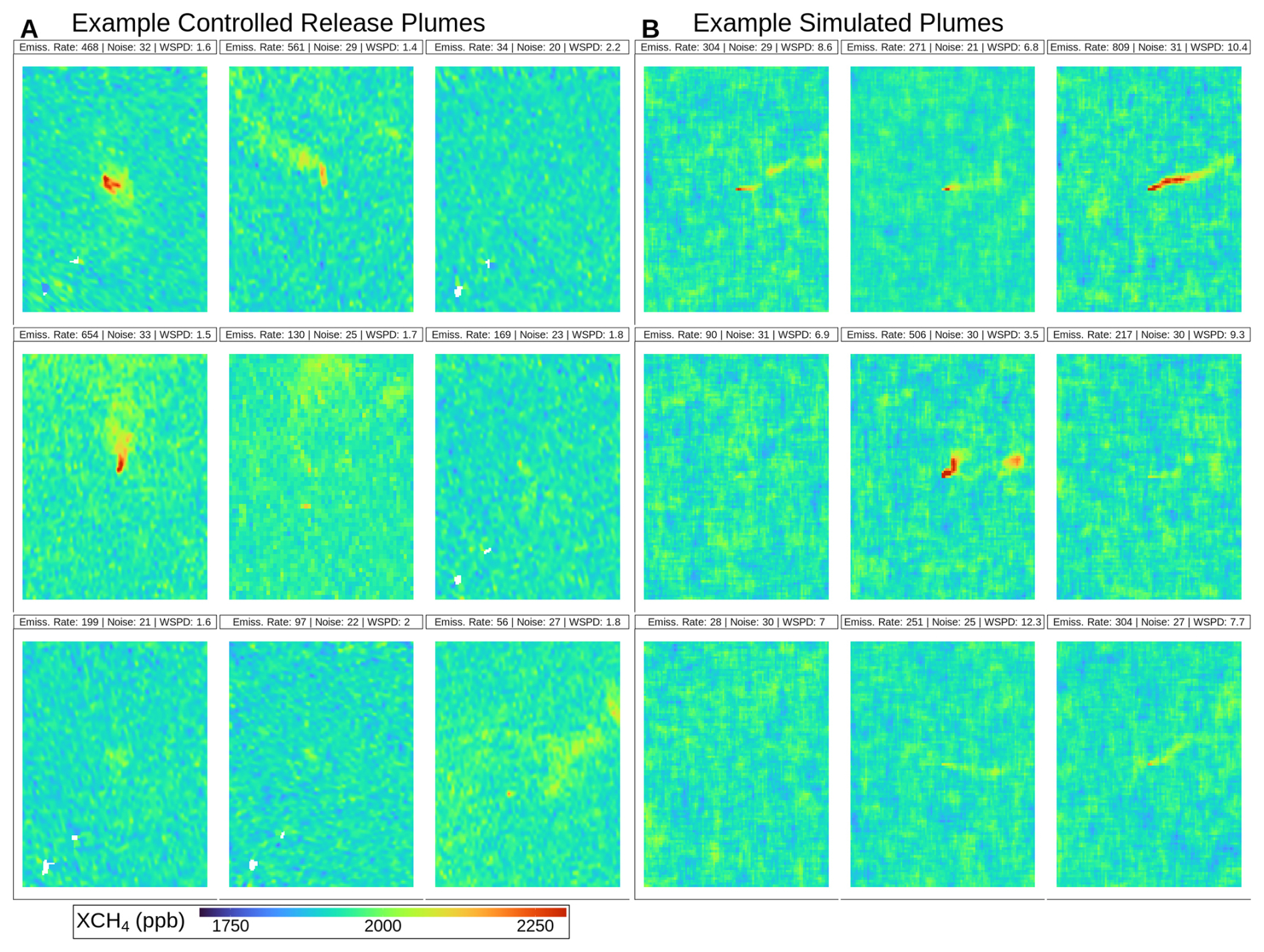
Figure 1 Example simulated plumes. Color represents XCH₄. Each plume has a different combination of emission rate (kg h⁻¹), pixel area (m²), gas concentration noise (ppb), and wind speed (m s⁻¹). (A) Scenes from controlled release experiments. (B) Scenes from simulated plumes.

To further extend the training scenes, we used image processing to change the emission rate, pixel area, and gas concentration noise of each of the 80 idealized WRF-LES scenes. First, we produced plumes of varying emission rates by scaling the XCH₄ of each pixel by the ratio of the original WRF-LES emission rate to the desired emission rate. This scaling relies on the linearity of CH₄ transport. Next, we aggregated pixels to vary their area. Finally, we added Gaussian noise, and a background XCH₄ value of 1800 ppb. Plume detection relies on contrast, and is not sensitive to the background value. The Gaussian noise included a spatial correlation between adjacent pixels of .7 to match the spatial correlation observed in MethaneAIR controlled release scenes. We did not vary cloud fraction or any other source of missing data in the simulated scenes. We do not explicitly vary aerosol optical depth, which varies with gas concentration noise. Each simulated scene contained only one source. This process generated a training data set of ∼ 80 000 simulated plumes. Figure 1 shows examples of the simulated plumes with different parameters.

We applied the same method of scaling noise and emission rate to controlled release scenes to create a more widely varying validation dataset. For MethaneAIR controlled release scenes, we scaled the XCH₄ values only within the plume, only for overpasses where the plume was successfully identified and masked. We scaled the XCH₄ values only within the masked area of the plume both up and down to vary the emission rate. We are also able to add Guassian noise to the scenes in the same way as the WRF-LES plumes. However, the wind speed of the controlled release scenes cannot be changed without changing the shape of the plume. Thus, these enhanced controlled release scenes have varying emission rate, pixel area, and gas concentration noise, but the same set of wind speeds as the original controlled release experiment.

2.4 Detection Algorithms

We analyzed two plume detection algorithms used by MethaneAIR and MethaneSAT, the divergence integral and wavelet methods. The divergence integral method uses Gauss's theorem to measure the amount of CH₄ leaving a small area (Chulakadabba et al., 2023; Warren et al., 2024). First, we threshold, where pixels 1.8 scene standard deviations above the mean XCH₄ value in the scene are retained. Next, thresholded pixels are clumped, where only pixels attached to clusters of at least 40 pixels are retained. Then, for each clump, a growing box Gaussian integral method is applied, where the wind speed and direction implied inflow and outflow of CH₄ across succesively larger boxes of pixels gives an emission rate and uncertainty for the plume (See Supplement of Chulakadabba et al., 2023 for full mathmatical details). If this emission rate is not positive to 1σ uncertainty, the clump is discarded. For more detail on the divergence integral method, see Chulakadabba et al. (2023). Adapted from medical imagery applications, the wavelet method isolates high frequency XCH₄ variation, interpreted as noise, and subtracts that structure from the observations. This leaves behind structured low frequency variation, interpreted as plumes. Further details on the wavelet algorthim can be found in Zhang et al. (2026). Both the divergence integral and wavelet are applied to both MethaneAIR and MethaneSAT observations.

We applied the plume detection algorithms to the training set of simulated plumes and recorded the successful and failed detections as binary outcomes. When generating the training data set, plume detection is fully automated; there is no manual quality assurance step to identify false positives, which are not a focus of this study. The main sources of false positives are terrain shadows, clouds/shadows, and surface albedo contrasts which will definitely not affect simulated plumes and almost definitely not affect controlled release scenes because of manual examination. A positive false positive rate seems to imply a positive P_d at q=0. However, P_d is defined as successful detection of a true plume, so by construction if q=0, then P_d=0. The plume observations from the MAIRX campaign are manually reviewed to remove false plume identifications (Warren et al., 2024). However, for a fully automated plume observation pipeline, not considering false positives would potentially bias with either sign, depending on what the most common false positive is. However, false plume identifications would not affect the P_d correction to the emissions distribution, which is the focus of this study.

We also analyze output from the Insight M algorithm used to detect plumes in LeakSurveyor scenes. Insight M provided the data required for our analysis from the 2022 Arizona controlled release experiment, including gas concentration noise, pixel area, and detection success. Their detection algorithm and controlled release scenes are not available to the public.

2.5 Logistic Regression on Parameterized Plume Observability

Following Bruno et al. (2024), we use a single log-linear form for g: for all systems and scenes

$$\begin{array}{}\text{(2)}& \text{Observability}\equiv g(q,a_{\mathrm{p}},\stackrel{\mathrm{̃}}{n},u)=\log \left({\displaystyle \frac{q}{\sqrt{a_{\mathrm{p}}}\stackrel{\mathrm{̃}}{n}u}}\right)\end{array}$$

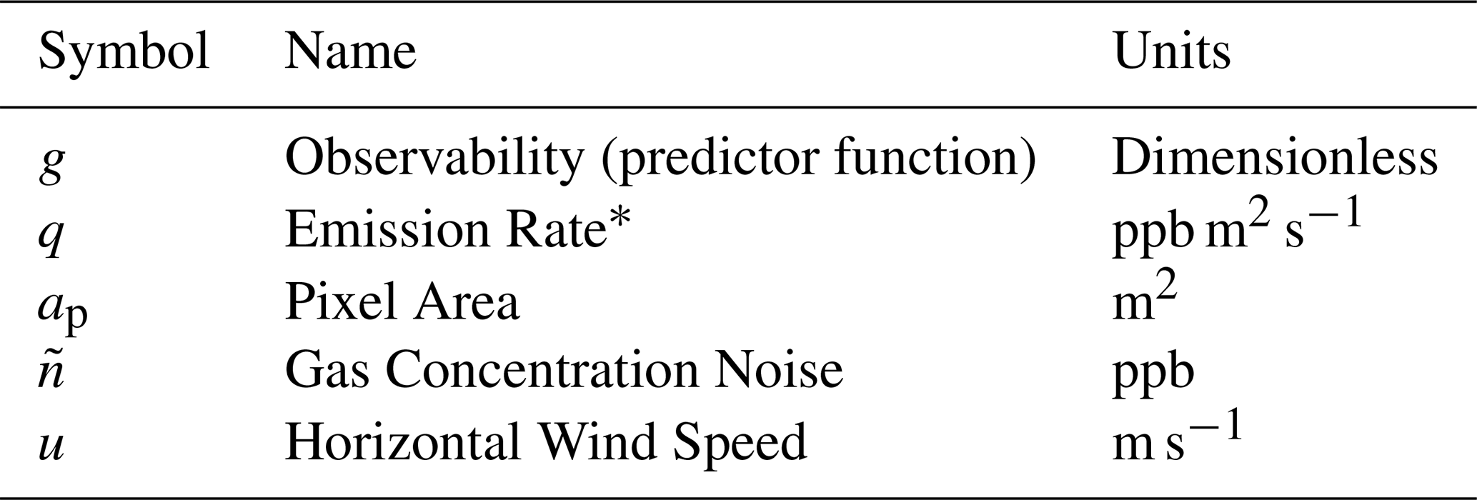
Table 2 Variables and units used in equation 2.

^* Here ppb refers to the enhancement of the column mean dry mole fraction (plume excess XCH₄). To convert to kg s⁻¹, multiply q by $M_{\mathrm{air}}/M_{{\mathrm{CH}}_{\mathrm{4}}}\times {\mathrm{10}}^{-\mathrm{9}}/g\times P_{\mathrm{surf}}\times (\mathrm{1}-{\mathrm{XH}}_{\mathrm{2}}\mathrm{O})$.

Observability g parameterizes the observing conditions and observing system characteristics into a single dimensionless term. Variable names and units for Eq. (2) can be found in Table 2. The lack of dimension enables ease of translation between observability space and relevant features like emission rate and wind speed. We expect the eddy scale wind speed to be the boundary of viability for the observability parameter. As such, this approach should not necessarily be applied to low wind night time conditions without further investigation. We further note that the observability parameterization is applicable to passive remote sensing systems, while active systems would require an additional scaling with the inverse square of observation altitude to account for power loss over distance. The observability link function is passed to the inverse function F, following Conrad et al. (2023). Differing from Conrad et al. (2023) and Thorpe et al. (2024), and following Bruno et al. (2024), we do not use different functional forms for F for different systems and release experiments.

We used a single, nondimensional form for two reasons: to enhance generalizability to systems without controlled release data, and to avoid overfitting. For example, a model trained with observability calculated for MethaneAIR scenes could be applied to MethaneSAT by recalculating observability based on the different pixel area and XCH₄ sensitivity. Tuning the functional form as well as the parameters will make a model that more closely fits training data than our form. However, we were concerned about overfitting to specific conditions, and preferred a less closely fitting model that is less likely to be an overfit. Thorpe et al. (2024) find that the more complex forms are robust to different observing conditions, however, this result is derived from controlled release data, which will always be limited in observing condition variety. In Fig. 2, we show that the models used in Conrad et al. (2023) and this paper do not perform significantly differently when applied to controlled release data.

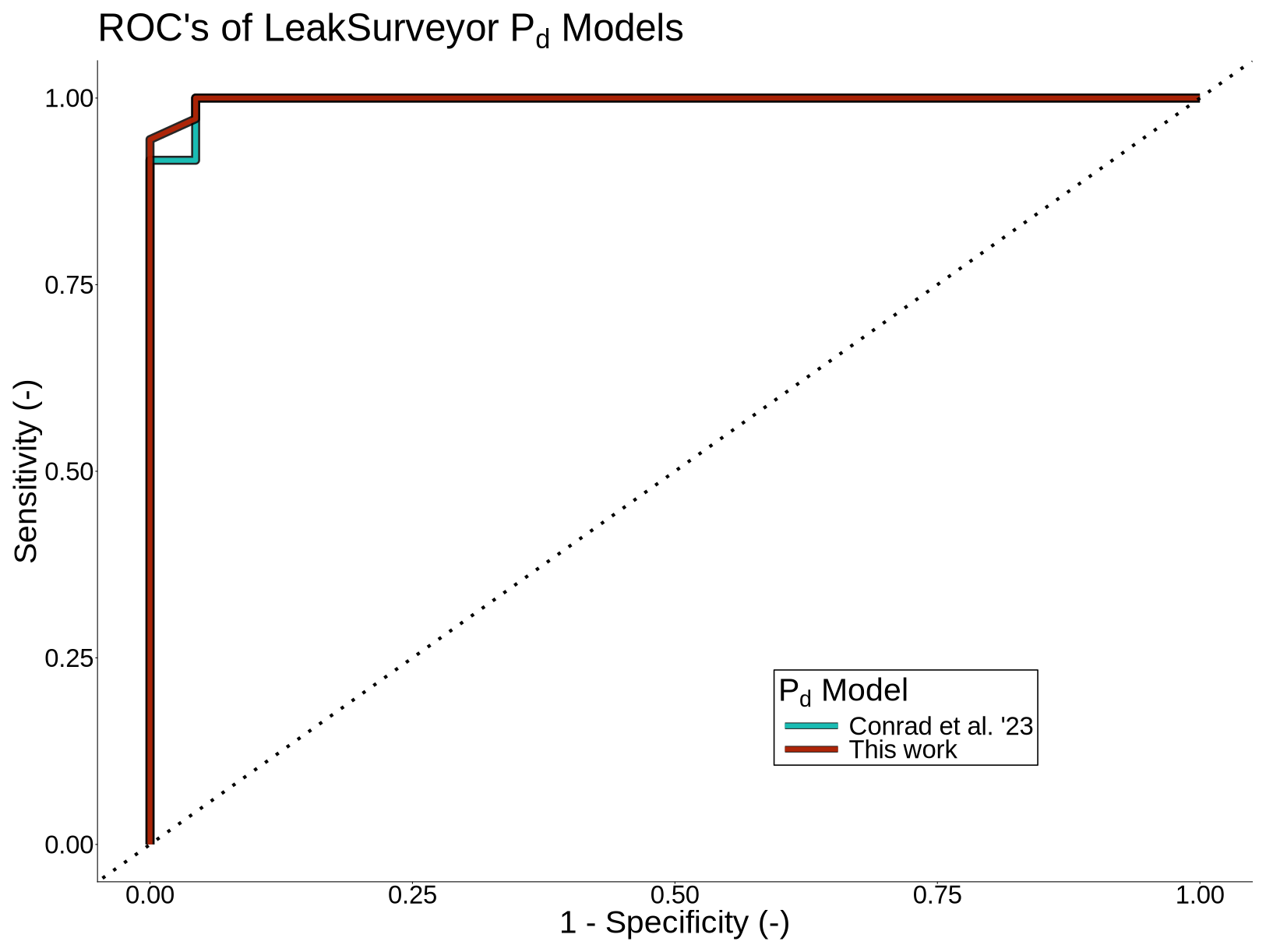
Figure 2 Receiver Operator Curve of fitted P_d models tested on controlled release data. X-axis is the true positive rate, or sensitivity, y-axis is the false positive rate, or the complement of specificity. Teal curve is for the model fitted by Conrad et al. (2023). Red curve is for the model fitted in this work.

Figure 2 shows receiver operator curves (ROC) generated by predicting P_d of LeakSurveyor's controlled release detection results from the 2022 controlled release using our methodology and Conrad et al. (2023)'s P_d model fit with 2021 controlled release data. Receiver operator curves are a commonly used tool for evaluating models of binary outcomes. Predictive skill of a model is captured by area of the ROC in sensitivity/specificity space above the 1:1 line, which represents an indiscriminate model. Our model has more area under the ROC than Conrad et al. (2023)'s, indicating more predictive skill. However, this difference is not statistically significant. This is because we only were able to use ∼ 100 controlled release overpasses from the 2022 Arizona controlled release for comparison of the two models. With more data, the two ROC's may diverge further. The Conrad et al. (2023) model is fit to the observing conditions of the 2021 controlled release experiment. Additionally, it was fit at the 2021 900 m observing altitude, while in 2022, they flew at a much lower altitude, resulting in a smaller native pixel area and higher P_d's. The best fit P_d model for Insight M reported in Table 2 of Conrad et al. (2023) (under the name Kairos) is

$$\begin{array}{}\text{(3)}& P_{\mathrm{d}}=\mathrm{1}-{\left(\mathrm{1}+{\left({\displaystyle \frac{\mathrm{8.5}\times {\mathrm{10}}^{-\mathrm{3}}{q}^{\mathrm{1.99}}}{(u+\mathrm{0.534}{)}^{\mathrm{1.92}}}}\right)}^{\mathrm{2}}\right)}^{-\mathrm{1.5}}\end{array}$$

This form does not have a term to adjust the observing altitude, pixel area, or gas concentration noise. Another fitted P_d model for partial detections by Insight M in the same table has the same functional form and does not include altitude or gas concentration noise. This demonstrates a potential pitfall in tuning the functional form of the P_d model to obtain the best possible fit with controlled release data.

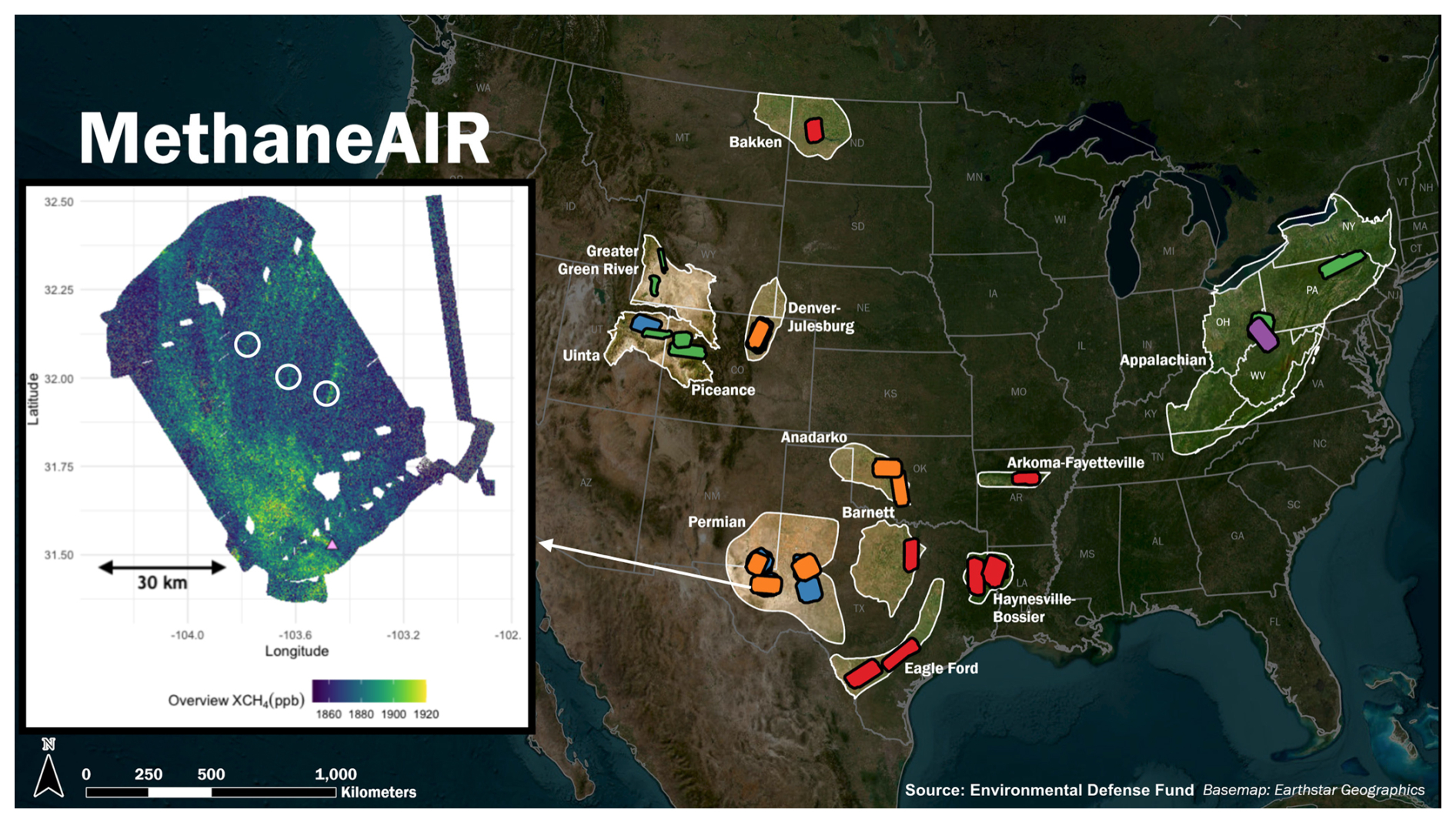
Figure 3 Map of MAIRX targets. Each colored shape is a flight pattern flown by MAIRX. The major oil and gas basins in the contiguous United States are marked. Inset: an example MAIR XCH₄ scene, in which large CH₄ plumes are circled in white. Each colored flight pattern on the map produced an XCH₄ scene like the inset example.

For fitting and validating P_d models, the emission rate q is known from a controlled release meter or prescribed when simulating the plume. For each scene, fitted P_d models predicted P_d for a range of emission rates. Pixel area is calculated from the XCH₄ scene. The gas concentration noise ($\stackrel{\mathrm{̃}}{n}$) contains noise contributions from the instrument as well as the observing conditions, including disturbances from upwind sources. For a given scene, $\stackrel{\mathrm{̃}}{n}$ is the standard deviation of the XCH₄ values of a “clean” portion of the scene. In this context, clean means that there is no variability from proximate emissions. Finding a clean portion of a scene can be done by visual inspection or by taking the pixels below an XCH₄ quantile cutoff. We collected the pixels below the 10th percentile. For a MAIR-E controlled release scene in Arizona with no proximal emissions, gas concentration noise shows low sensitivity to the choice of XCH₄ quantile (Fig. A1). Clean portions of scenes can be found in many ways, but they are confirmed clean by checking that the XCH₄ values are normally distributed for the pixels selected. This means that clean XCH₄ pixels are unstructured, but unaffected by local emissions. Proximate emissions are a valid source of gas concentration noise – it is harder to identify a plume in a scene with many sources than a plume from an isolated source. In large scenes, there may be multiple gas concentration noise values, in which case a more accurate P_d may be calculated by considering subscenes. We used wind speed measured by the anemometer at the controlled release site (Chulakadabba et al., 2023). To predict P_d with a fitted model for MAIRX scenes, we used the lowest-level High Resolution Rapid Refresh (HRRR) winds averaged for each scene.

We calculated observability for each simulated training scene. Then, we fitted a logistic regression on the binary successful/failed detection outcome of the wavelet and divergence integral detection algorithms applied to the simulated scenes.

2.6 MAIRX Steady State Emissions Distribution

In the summer of 2023, MethaneAIR flew the MAIRX observation campaign. It covered ∼ 80 % of the oil and gas production in the continental United States (Warren et al., 2024). Figure 3 shows the MAIRX targets over the Permian and contiguous United States. Plumes were detected via the wavelet and divergence integral methods, and their emission rates quantified by divergence integral (Chulakadabba et al., 2023; Warren et al., 2024). The emissions distribution was calculated following the ergodic, or steady state assumption (Sherwin et al., 2024). The steady state assumption posits a constant underlying distribution of plumes, which can be approximated given enough samples. This will produce distributions that do not take source persistence into account. In addition to CH₄ plumes, MethaneAIR also observes regional XCH₄ gradients, which can be used to infer dispersed emissions. Dispersed emissions can be thought of as the regional XCH₄ enhancement due to the combination of plumes too small to be detected as a discrete sources and larger plumes that have spread out after the source has stopped emitting. We quantify these emissions using an inverse method that combines gridded area enhancements with an atmospheric transport model, Stochastic Time Integrated Lagrangian Transport (Lin et al., 2003; MacKay et al., 2026).

We apply our analysis of the effects of P_d on inferred emissions distributions to the example of the Permian Basin, and an analysis of other N. American basins. We took the average dispersed emissions estimate of all the valid scenes for each MAIRX sampled basin. The total emissions were defined as the sum of all plume and dispersed emissions. The emissions distribution was defined as the fraction of total emissions associated with plumes of different binned emission rates. To investigate the effects of P_d of different systems on the emissions distribution, we performed Monte Carlo simulation of the analysis. For 1000 simulations, we resampled with replacement from the MAIRX observed plumes, with quantified emission rates. We then calculated the cumulative fraction of total emissions (plume emisssions + area emissions) due at a spectrum of emission rates, We included a Gaussian error term to represent uncertainty in the area emissions, with zero mean and standard deviation equal to the sample standard deviation, if MAIRX included more than three scenes in a given basin. To aggregate the results we took the mean of all realizations, and to quantify uncertainty, we set the confidence interval as the middle 95 % quantile.

Additionally, we calculated P_d using our fitted models, gas concentration noises and wind speeds from MAIRX scene. This enabled an emissions distribution with a P_d correction term, as described in the introduction. We examined MethaneAIR, MethaneSAT, and a hypothetical satellite with the same spatial resolution as MethaneSAT but worse CH₄ sensitivity, represented by a higher nominal gas concentration noise. We calculated the P_d of these three systems for all observed emission rates for each MAIRX scene, and generated bootstrap samples from MethaneAIR observed plumes. In this analysis, we used the probability of either method detecting the plume $P_{\mathrm{d}}=\mathrm{1}-\left(\mathrm{1}-P_{\mathrm{d}}^{\text{div.int.}}\right)\left(\mathrm{1}-P_{\mathrm{d}}^{\text{wave.}}\right)$. To simulate the observations of MethaneSAT and the hypothetical satellite, each plume was included in the bootstrap sample with probability P_d.

3 Results and Discussion

3.1 Probability of Detection Model

Figure 4 shows the validation comparison for MethaneAIR, using the model trained on the LES simulations. Each point represents image processed controlled release data binned by detection rate. The divergence integral algorithm's P_d model best fit line has a slope of 1.22, an intercept of 0.05, and an adjusted R² of 0.83. The wavelet algorithm's P_d model's best fit line has a slope of 0.91, an intercept of 0.36, and an adjusted R² of 0.99. The P_d model works well for the wavelet algorithm applied to MethaneAIR data, but not as well for the divergence integral algorithm. The difficulty for the divergence integral algorithm likely reflects its sensitivity to missing data, which were not present in the training set. This is because the divergence integral algorithm needs intact boxes of XCH₄ pixels of various sizes within the scene, while the wavelet does not. For example, clouds prevent imaging spectrometers from measuring reflected solar light, and leave regions of missing data in real XCH₄ scenes. We did not validate P_d model performance for either Insight M or MethaneSAT, because we did not have access to controlled XCH₄ images.

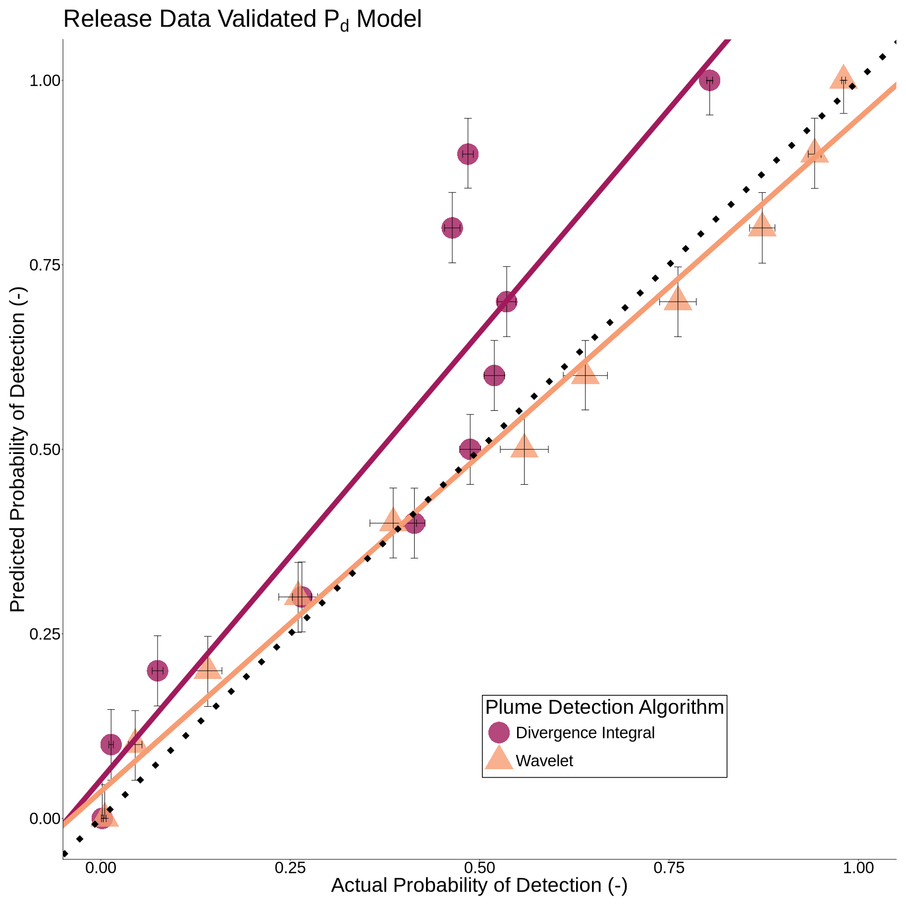
Figure 4 Validation of the probability of detection model using multiplexed affected release plumes and two detection algorithms: divergence integral and wavelet. Each point represents the binned model predicted detection rate (x-axis) compared with the true probability of detection (y-axis). Uncertainty estimates are derived from the binomial central limit theorem. The dotted 1:1 line represents perfect agreement between model predicted and validation P_d. Points above the dotted line represent the model overestimating the probability of detection. The thin colored lines are the best fit lines for each of the detection algorithms.

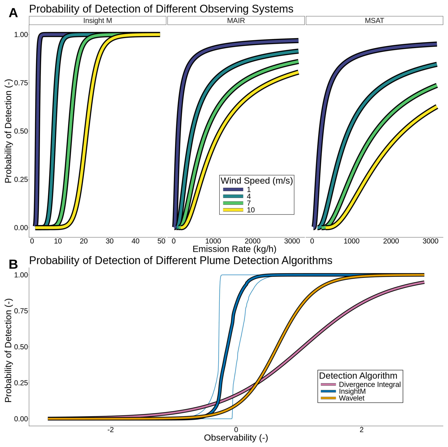
Figure 5 (A) Intercomparison of probability of detection between different observing systems (MethaneAIR, MethaneSAT, Insight M) for a range of emission rates and wind speeds. Gas concentration noise was set to the system average for controlled release scenes (MethaneAIR, LeakSurveyor™) or a sample of observational scenes (MethaneSAT). For MethaneAIR and MethaneSAT, the reported P_d is for the wavelet algorithm. (B) P_d curves for divergence integral, wavelet, and proprietary LeakSurveyor algorithm in observability space. Thick lines are the mean and thin lines are the 95 % CI inferred via bootstrap.

3.2 Observing System Intercomparison

Our probability of detection model quantifies the differences in plume detection capabilities between observing systems and detection algorithms. Figure 5A shows P_d curves modeled for various emission rates and wind speeds for LeakSurveyor™, MethaneAIR, and MethaneSAT. As anticipated, LeakSurveyor's™ lower observation altitude allows it to detect lower emission rate plumes with higher probability than MethaneAIR or MethaneSAT.

In the MAIRX campaign, wind speed controlled P_d more than gas concentration noise. This might not be true for other observing systems with less sensitivity to XCH₄. Although controlled release data for MethaneSAT is not available, g enables prediction of P_d for the divergence integral and wavelet algorithms applied to MethaneSAT scenes. The predicted difference in P_d between MethaneAIR and MethaneSAT is relatively small at low wind speeds compared to high wind speeds. The coarser spatial resolution of MethaneSAT is compensated by higher sensitivity to XCH₄, resulting in lower GCN, and slightly higher P_d.

Because observability normalizes for all observing system features apart from the algorithm, P_d curves in observability space can be used to compare the skill of plume detection algorithms. Figure 5B shows the P_d curves from three different plume detection algorithms. These curves are fitted using simulated XCH₄ scenes (divergence integral and wavelet) and controlled release trials (Insight M). The wavelet algorithm performs better on simulated plumes than the divergence integral. When applied to scenes from the MAIRX campaign, the wavelet algorithm also found more plumes and more low emission rate plumes. The Insight M algorithm and controlled release XCH₄ images are proprietary, and we were not able to fit a P_d model to simulated plumes like we were for the divergence integral and wavelet. However, by calculating the observability of the controlled release plumes, we are able to compare the divergence integral, wavelet, and Insight M algorithms.

Figure 5 suggests that proprietary Insight M plume detection algorithms are slightly more skillful than the divergence integral and wavelet, independent of the lower observation altitude of Insight M XCH₄ images. However, because the Insight M P_d was only fit on limited controlled release scenes, and the detection algorithms and XCH₄ images are proprietary, a complete analysis is impossible. The Insight M probability of detection curve has much higher uncertainty than the other algorithms' curves because it is derived from ∼ 100 controlled release scenes rather than ∼ 80 000 simulated scenes. Ideally, Insight M images and algorithms would be available for testing. However, our method offers the next best alternative to isolate the effects of detection algorithm, spectrometer, and altitude on P_d.

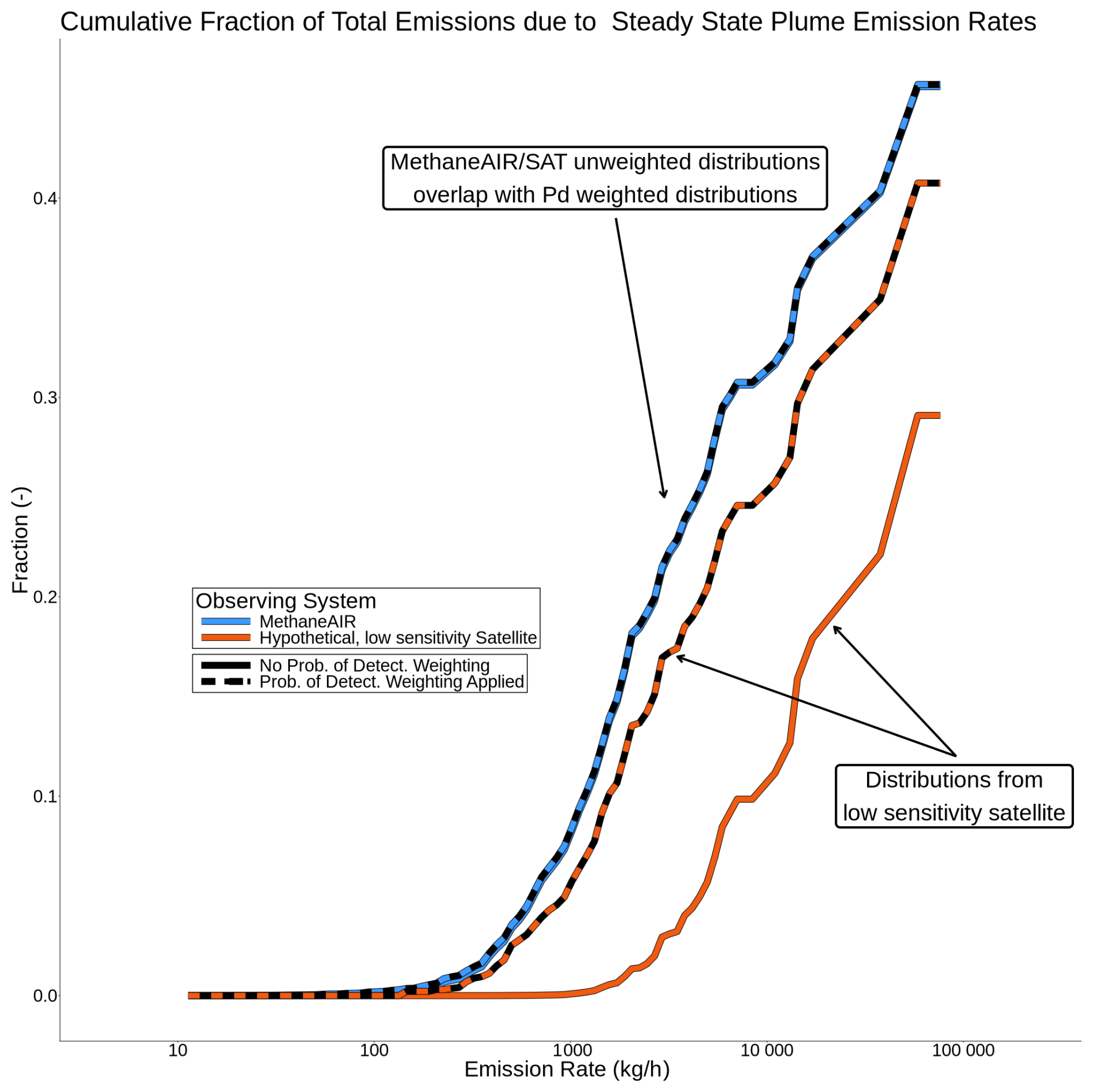
Figure 6 Steady state cumulative fractional contributions to total emissions (y-axis) of events of different emission rates (x-axis) observed in the Permian, during MAIRX. Distributions are colored to indicate observing system. Dashed distributions include P_d weighting, solid distributions do not. For uncertainties, see Table 3.

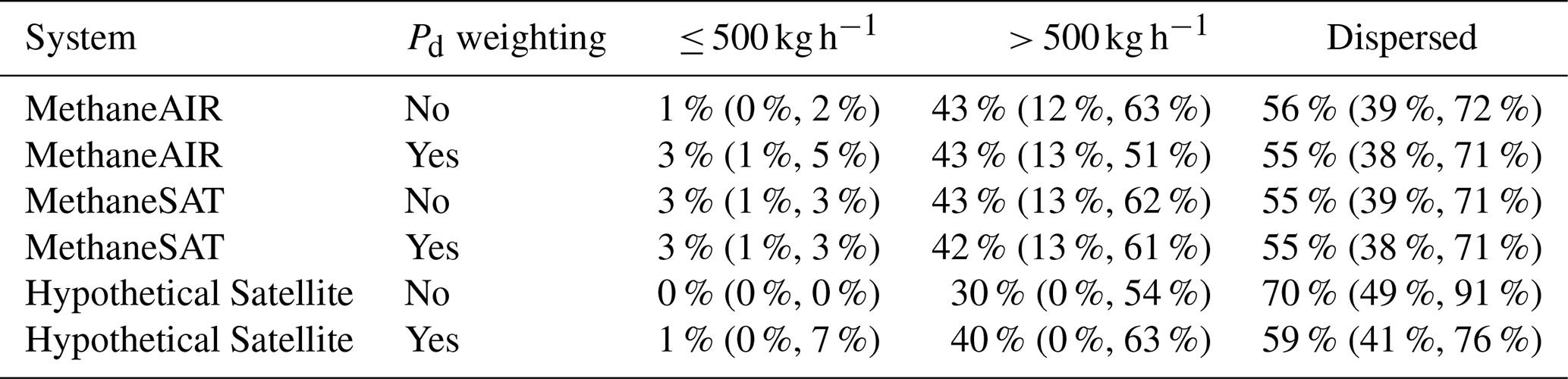
Table 3 Fraction of Total Permian Emissions Due to Small and Large Plumes, and Dispersed Emissions, During MAIRX.

3.3 MAIRX Steady State Emissions Distribution

Figure 6 shows the observed cumulative emissions distributions for MAIRX, and distributions from simulated observations from MethaneSAT and a hypothetical satellite with the same spatial resolution as MethaneSAT but lower XCH₄ sensitivity. Each system has two observed emission distributions, one with P_d weighting (dashed) and one without (solid). Figure 6 shows how including a P_d reduces the heaviness of the tail of the emission rate distribution. Due to heavy tailed oil and gas emissions distributions, the value of an accurate model of the probability of detection increases with higher detection thresholds.

Table 3 contains the fraction of total emissions attributed to plumes < 500 kg h⁻¹, plumes > 500 kg h⁻¹, and dispersed emissions, for each observing system. The dispersed emissions represent CH₄ from current plumes too small to be detected and from extinct plumes that have dispersed. For MethaneAIR, there is close agreement between the cumulative distribution with P_d weighting and the one without, indicating that measurements capture the most significant plumes. The P_d term shifts a small fractional contribution of ∼ 1 % from dispersed emissions to plumes < 500 kg h⁻¹ (Table 3). These results indicate that for the Permian, an observing system with a nominal P_d inflecting in the hundreds of kg h⁻¹ CH₄ range is sufficient for characterizing the small population of plumes > 500 kg h⁻¹ that control total plume associated emissions. This assessment is contingent on well constrained dispersed emissions – in this case, generated by MethaneAIR. MethaneSAT has coarser spatial resolution than MethaneAIR, but higher XCH₄ sensitivity, resulting in a lower average scene gas concentration noise. It retains the ability to detect moderate plumes, inflecting at ∼ 500 kg h⁻¹ compared to MethaneAIR's ∼ 200 kg h⁻¹ at 5 m s⁻¹ wind speed (Fig. 5A). This difference in P_d is not enough for P_d to materially affect the inferred contribution of emission rates > 500 kg h⁻¹ to total emissions.

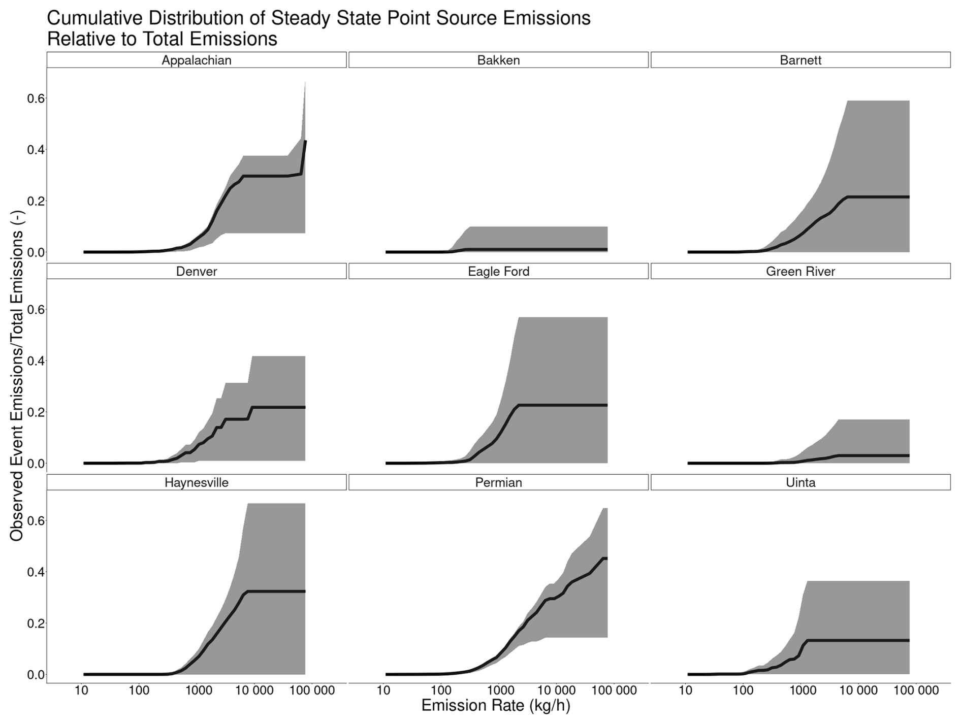
Figure 7 North American oil and gas basins cumulative emission rate distributions. Steady state cumulative fractional contributions to total emissions (y-axis) of events of different emission rates (x-axis) observed in each basin. The grey intervals are the 95 % confidence interval inferred from Monte Carlo simulations.

We also analyze a hypothetical satellite with lower XCH₄ sensitivity to show a case where the P_d term is important. The lower XCH₄ sensitivity is reflected in a higher characteristic gas concentration noise (∼ 10 ppb) than MethaneSAT (∼ 100 ppb), but the same pixel area. This is an excercise to demonstrate that P_d is relevant to emissions distributions when the observing system no longer has near perfect detection of emission rates above 500 kg h⁻¹ . The choice to change gas concentration noise to achieve this effect is arbitrary, and the hypothetical satellite is not meant to represent any particular real world satellite, though the result is generalizable to satellites without perfect detection above 500 kg h⁻¹. In Fig. 6, the distribution produced by the hypothetical lower sensitivity instrument (orange) diverges from those produced by the higher sensitivity instruments (yellow and blue). However, the P_d weighted distribution (dashed orange) is more similar to the “ground truth” from MethaneAIR (yellow), indicating that the P_d term recovers most of the missed emissions from both large and small plumes (Table 3). However, these P_d weighted estimates have much wider CI's, (0 %–63 % of total emissions from > 500 kg h⁻¹ compared to 12 %–63 % for MethaneAIR) due to fewer plume observations. Pandey et al. (2024) also note P_d controlled transfer between dispersed and plume emissions. Analysis of low XCH₄ sensitivity systems is relevant to projects attempting to detect CH₄ plumes with multispectral satellites, which may only have one radiation band with CH₄ absorption, such as Rouet-Leduc and Hulbert (2024).

Our estimated emissions distributions differ from a different analysis of MethaneAIR plume observations of the Permian (Warren et al., 2024). We find a higher fraction of total emissions due to plumes. One explanantion is that Warren et al. (2024) only used plumes detected by the divergence integral, while we included both wavelet and divergence integral detected plumes. Additionally, Warren et al. (2024) use a persistence weighting approach (Cusworth et al., 2021). Persistence weighting accounts for intermittency of sources by multiplying their steady state emission rate by $\frac{N_{\mathrm{e}}}{N_{\mathrm{o}}}$, where N_e is the number of times the source was observed emitting and N_o is the number of times it was observed. This would decrease the inferred fraction of total emission from plumes.

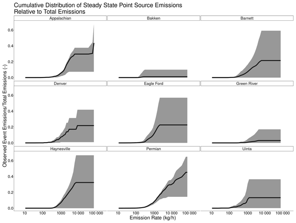
In our consideration of the effect of P_d on emissions distributions, we adopted the steady state assumption. In the Permian, there are large uncertainties in the steady state fraction of emissions attributable to rare, high emission rate events (Table 3). This result is generalizable to other North American basins. In Figure 7, we show MAIRX derived emissions distributions for the North American oil and gas basins shown in Fig. 3. The confidence intervals are derived using the same Monte Carlo method described in Sect. 2.6, without a P_d correction. We do not attempt to estimate contributions or uncertanties for unobserved emission rates, resulting in the discontinuities in the curves in Fig. 7.

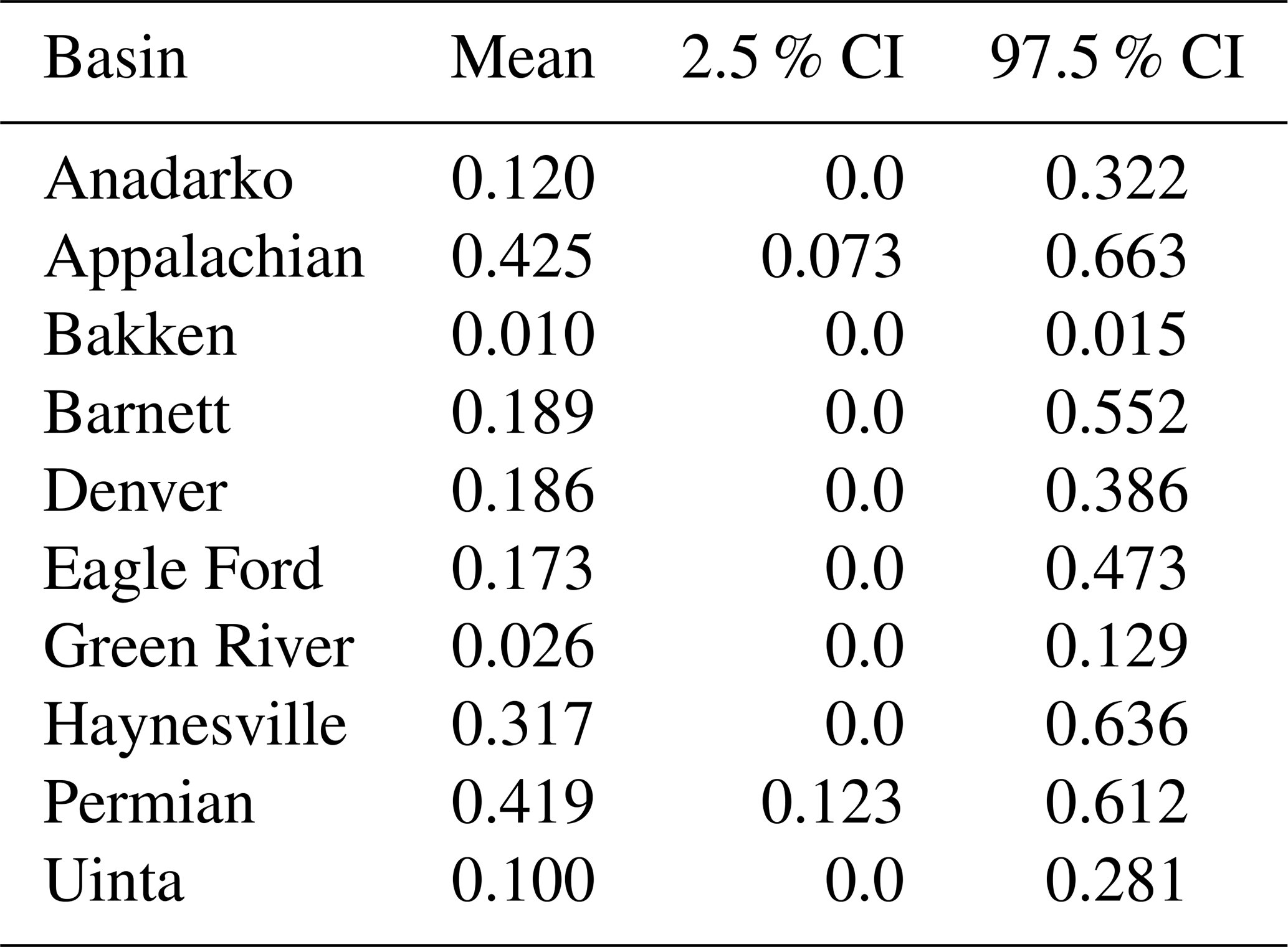
Based on the contributions from high emission rate events, the basins can be divided into three groups: possibly dominant, at most moderate, and negligible. Table 4 shows the fraction from each, and confidence intervals derived using the same Monte Carlo method described in Sect. 2.6. The possibly dominant group includes the Permian, Appalachian, Haynesville, and Barnett basins. In these basins, the 97.5 % CI contribution from high emission rate events is more than half of the basin total. However, the 2.5 % CI's of basins in this group are less than 10 %. Anadarko, Denver, Eagle Ford, and Uinta make up the moderate group. Their 97.5 % CI's are more than 25 % but less than 50 %. Green River and Bakken had negligible contributions from high emission rate events, with the 97.5 % CI less than 10 %. Apart from the Bakken, all of the studied basins are poorly constrained – they have CI's going from more than .1 to less than 1.5 times the mean.

Table 4 The fraction of total basin emissions due to emission events with emission rate greater than 500 kg h⁻¹. 95 % Confidence intervals inferred via bootstrap.

The Monte Carlo uncertainties in Fig. 7 indicate that the total emissions are sensitive to small shifts in the steady state prevalence of high emission rate events. This is a manifestation of the heavy tailed oil and gas CH₄ emission rate distribution (Brandt et al., 2016). The uncertainties from the frequencies of rare high impact emission events are larger than the change in emissions distribution due to the P_d correction for MethaneAIR in Fig. 6. The cumulative contribution curves of all of these basins begin to rapidly rise beyond ∼ 500 kg h⁻¹, before flattening abruptly beyond the maximum observed emission rate. Is it reasonable to expect that the true underlying emission rate distribution contains zero probability for emission rates beyond the maximum MAIRX observed? Indeed, in Fig. 7, the cumulative contribution curves of the moderate basins could be expected to converge to the curves of the possibly dominant basins with more observations. It is not clear how many repeat observations of the same domain are needed for a steady state model to reliably recover the true emissions distribution. In light of high uncertainties around the frequency of rare events and differences with emissions distributions that incorporate persistence weighting (Warren et al., 2024), a more complex model of the frequency and durations of high emission rate plumes may be justified.

4 Conclusions

Probability of detection is critical for interpretation of observations of plumes and inference of emissions distributions. Controlled release data should still be considered a gold standard for estimating P_d. Our approach to modeling P_d does not require controlled release data, which makes it is particularly relevant to planning future missions and systems without controlled release data, such as MethaneSAT. The simulated plume approach also allows for consideration of higher variability in observing conditions. Our approach could also be used to predict the probability of detection of plumes of gasses other than CH₄, such as carbon dioxide plumes emitted by combustion power plants. This study demonstrates the value of simultaneously estimating emissions from plumes and area emissions, which enable estimating aggregated emissions from undetectable plumes.

We find that considering P_d increases in importantance as the observing system decreases in sensitivity to plumes. For systems that can capture 500 kg h⁻¹ with high P_d, the emission rates heavy tail means that coverage and area emissions capability are more important than driving down emission rate detection thresholds. We find that uncertainty in emissions distributions in North American basins is driven more by frequency of rare high impact events than ability to constrain. Future work should more deeply evaluate uncertainties associated with the steady state assumption and persistence weighting method.

Appendix A

Table A1 Fitted Logistic Regression Parameters for MethaneAIR, MethaneSAT, and Insight M.

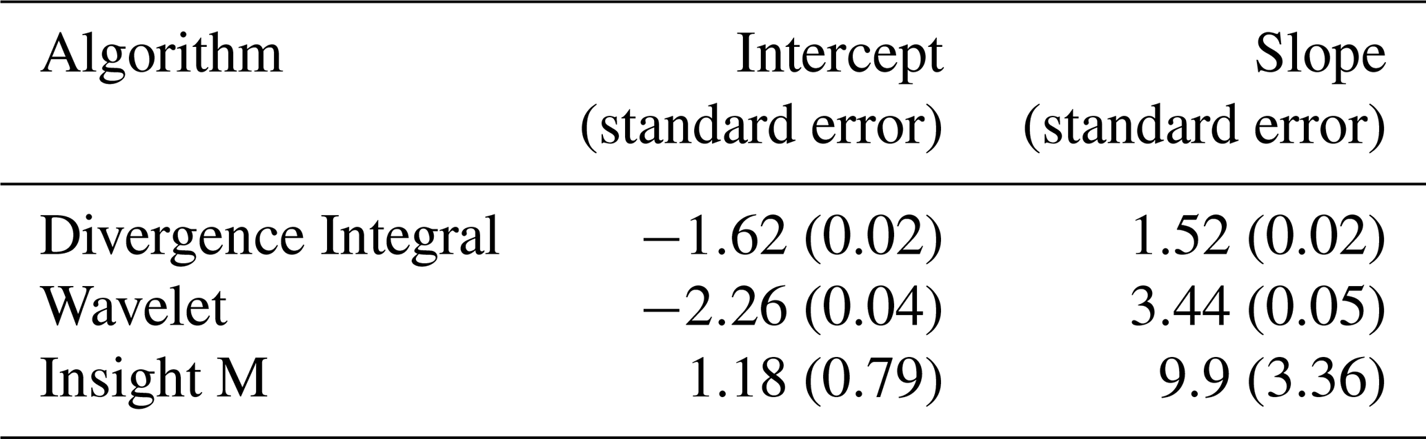
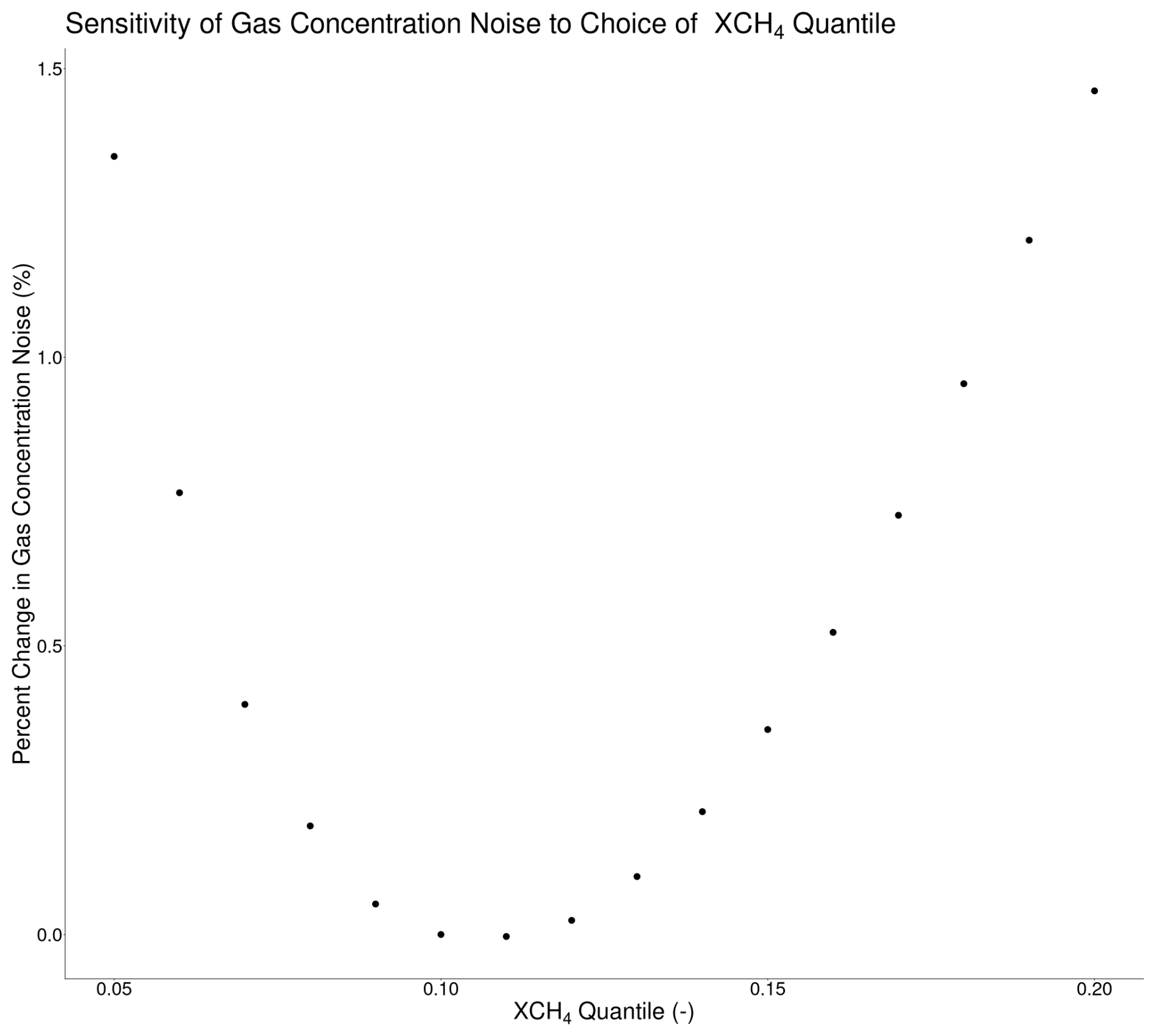
Figure A1 The sensitivity of gas concentration noise, in percent change from a baseline XCH₄ quantile of 0.1 (y-axis), to the choice of XCH₄ quantile used to define the clean background (x-axis). This curve is derived from a MAIR-E 2022 controlled release overpass, with no proximal CH₄ sources.