Assessing the consistency of XCO₂ products from DQ-1 ACDL and passive satellites using a unified comparison framework

Da Qi-1 (DQ-1) carries the Aerosol and Carbon Dioxide Lidar (ACDL), a spaceborne integrated path differential absorption (IPDA) lidar that retrieves the column-averaged dry-air mole fraction of carbon dioxide (XCO₂) using active laser measurements. Unlike passive near-infrared/shortwave-infrared sensors that rely on reflected sunlight, ACDL can observe at night and high latitudes, but its sampling and effective column definition differ from passive XCO₂ products. Evaluation is therefore needed before active and passive observations can be interpreted jointly. We compare DQ-1 ACDL with the Orbiting Carbon Observatory (OCO-2 and OCO-3) and Greenhouse gases Observing SATellite (GOSAT and GOSAT-2) missions from June 2022–December 2024 using a unified framework that combines Copernicus Atmosphere Monitoring Service (CAMS)-based coherence assessment, sampling availability, daily 2° aggregation, spatiotemporal collocation, and correction for XCO₂ column-definition differences. Validation against the Total Carbon Column Observing Network (TCCON) gives R=0.92, a mean bias of 0.21 ppm, and a root-mean-square error (RMSE) of 1.49 ppm for daytime DQ-1, comparable to GOSAT. Over coherent and well-sampled regions, DQ-1 is broadly consistent with OCO-2 and OCO-3, with mean differences generally below 0.5 ppm and similar spatial and meridional structures. Over ocean, the DQ-1–OCO differences vary with surface reflectance and wind speed, with different reflectance relationships for OCO-2 and OCO-3. Nighttime DQ-1 is also broadly consistent with CAMS-derived XCO₂. Regional analyses show complementary DQ-1 coverage where passive observations are limited. These results support DQ-1 ACDL as a quantitatively comparable and complementary component of the satellite XCO₂ observing system.

1 Introduction

The continued accumulation of atmospheric carbon dioxide (CO₂) is one of the primary drivers of anthropogenic climate change and is a key variable for characterizing changes in the global carbon cycle, constraining surface sources and sinks, and assessing emission changes (Friedlingstein et al., 2026). Due to the high background concentration of atmospheric CO₂, perturbations caused by surface fluxes and atmospheric transport are typically only of ppm magnitude. Therefore, carbon-budget assessments, source–sink attribution, and emission estimates all rely on CO₂ observations with high precision and accuracy (Crowell et al., 2018; Kulawik et al., 2016). Ground-based observations provide high precision and temporal continuity and serve as an important foundation for carbon-cycle studies and satellite validation. However, their spatial coverage is limited and unevenly distributed. Satellite observations of the column-averaged dry-air mole fraction of CO₂ (XCO₂) can provide broader spatial coverage than ground-based observations and be assimilated into atmospheric inversion systems to constrain and quantify natural CO₂ fluxes and anthropogenic CO₂ emissions (Basu et al., 2018; Buchwitz et al., 2017; Keppel-Aleks et al., 2013; Wunch et al., 2011). Beyond regional carbon-cycle applications, satellite XCO₂ observations are also being explored for emission monitoring, with high-resolution observations providing complementary capabilities for facility-scale quantification (Han et al., 2026; Zhang et al., 2026).

Over the past two decades, passive satellite observations based on solar-reflected near-infrared and shortwave-infrared (NIR/SWIR) spectra have developed into a relatively mature XCO₂ observing system and have become an important reference for evaluating new CO₂ remote-sensing techniques. The development of missions from SCIAMACHY to GOSAT, OCO-2/OCO-3, GOSAT-2, and TanSat has continuously improved global XCO₂ observing capability, retrieval algorithms, and the validation framework based on the Total Carbon Column Observing Network (TCCON) (Buchwitz et al., 2005; Kuze et al., 2016; Noël et al., 2021, 2022; O'Dell et al., 2018; Taylor et al., 2023; Yang et al., 2020). However, passive NIR/SWIR retrievals rely on radiance reflected by the surface or cloud tops under solar illumination, and their data availability and retrieval errors are influenced by solar zenith angle, surface reflectance, clouds and aerosols, and quality control. For example, although OCO-2 can acquire nearly one million soundings per day, typically only about 7 %–12 % of these soundings are retained after quality control and used for XCO₂ retrieval on monthly timescales (Crisp et al., 2017). Therefore, differences among passive XCO₂ products cannot be attributed simply to sensor biases. They usually reflect the combined effects of retrieval algorithms, quality control, sampling representativeness, and bias correction.

Active CO₂ remote sensing based on integrated path differential absorption (IPDA) lidar provides a physically distinct approach to XCO₂ observation compared with passive remote sensing based on reflected sunlight. This technique has been systematically investigated in earlier mission concepts and airborne demonstrations, including ASCENDS and A-SCOPE (Abshire et al., 2010, 2014; Amediek et al., 2017; Wang et al., 2014). For China's CO₂-IPDA satellite mission, previous studies have assessed instrument performance and the feasibility of urban CO₂ detection (Han et al., 2017, 2018). In April 2022, the Aerosol and Carbon Dioxide Lidar (ACDL) onboard the Atmospheric Environment Monitoring Satellite Da Qi-1 (DQ-1) was launched into orbit, bringing spaceborne active IPDA CO₂ sensing into on-orbit application. The CO₂ channel of ACDL operates near 1.57 µm and retrieves XCO₂ by measuring differential CO₂ absorption along the optical path with online and offline laser pulses (Mao et al., 2018; Zhang et al., 2024). For each CO₂-IPDA measurement, the online and offline laser pulses propagate through the atmosphere and are reflected by a hard target, typically the surface or an optically thick cloud top, before the return signals are collected by the telescope. Their differential attenuation therefore provides an integrated differential absorption optical depth along the two-way path. Although the lidar return is range resolved for locating the reflecting target, the CO₂ absorption measurement is path integrated and does not provide independent layer-by-layer CO₂ information; instead, the ACDL weighting function describes the vertical sensitivity of the integrated column measurement, from which XCO₂ is retrieved (Shi et al., 2023; Han et al., 2025). Because its active light source does not depend on solar illumination, ACDL has potential sampling advantages at night and at high latitudes, providing observations under conditions in which passive NIR/SWIR measurements are limited by solar illumination (Wang et al., 2014). Recent studies have reported the XCO₂ retrieval framework, global XCO₂ observation characteristics, and validation of DQ-1 ACDL against TCCON and passive satellite products, and have demonstrated its potential for diagnosing strong point sources, urban fossil-fuel CO₂ emissions, and power-plant emissions (Han et al., 2024, 2025; Shi et al., 2023; Yi et al., 2025, 2026; Zhang et al., 2024; Zhang et al., 2025). However, ACDL is not a simple alternative to passive NIR/SWIR sensors for XCO₂ measurements. They differ systematically in light-source dependence, footprint scale, day–night sampling, vertical sensitivity, and effective column definition. As a result, differences between their XCO₂ products may reflect contributions from real atmospheric variability, sampling representativeness, and observation-operator differences.

Beyond the independent validation of individual XCO₂ products, a more critical question is how active and passive XCO₂ products can be compared within a unified measurement-definition and sampling framework. Previous studies have examined the retrieval and validation of GOSAT/GOSAT-2 products (Noël et al., 2021, 2022), the consistency of OCO-2 and OCO-3 (Taylor et al., 2023), intercomparisons among multiple passive XCO₂ products (Fang et al., 2023; Kong et al., 2019; Liang et al., 2017; Yoshida et al., 2013), and the validation and emission applications of DQ-1 ACDL products (Han et al., 2024, 2025; Zhang et al., 2024; Zhang et al., 2025). These studies provide an important basis for understanding the error characteristics and application potential of different XCO₂ products. To our knowledge, no previous study has systematically compared DQ-1 ACDL with OCO-2, OCO-3, GOSAT, and GOSAT-2 within a unified active–passive framework that jointly accounts for background-field coherence, multi-satellite sampling availability, spatiotemporal collocation, and XCO₂ column-definition differences. This unified framework provides a consistent basis for interpreting inter-product differences between active and passive satellite XCO₂ observations.

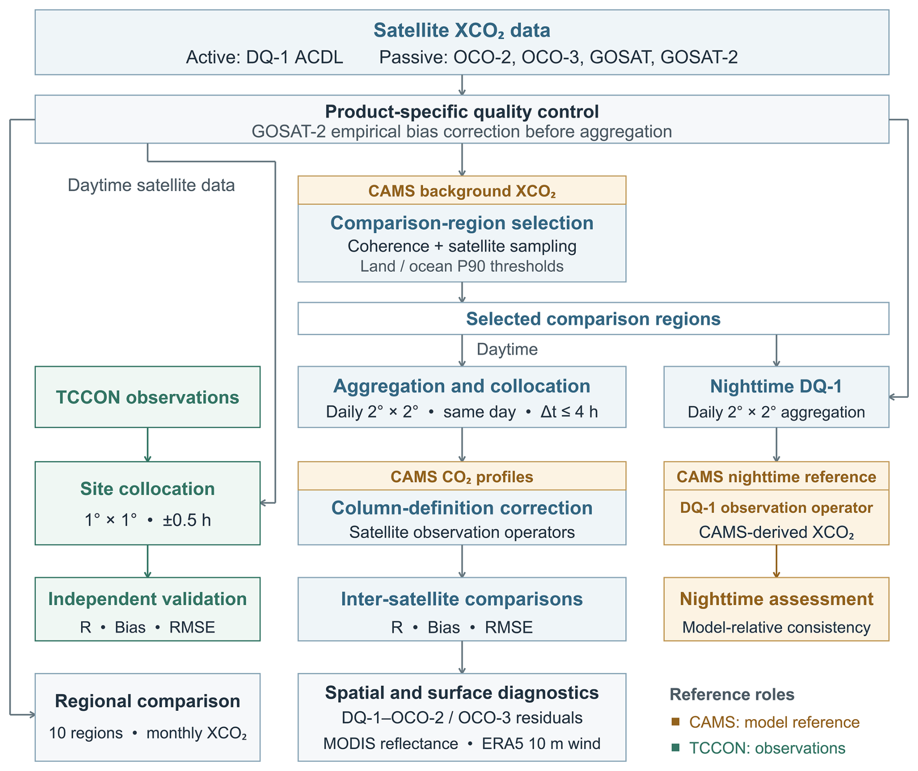
In this study, we compare DQ-1 ACDL with OCO-2, OCO-3, GOSAT, and GOSAT-2 XCO₂ products from June 2022–December 2024 within a unified active–passive framework. We first identify coherent and well-sampled comparison regions, evaluate the satellite products against TCCON, and quantify inter-satellite consistency after daily 2° aggregation, collocation, and correction for XCO₂ column-definition differences. We then diagnose the remaining regional differences, assess nighttime DQ-1 against CAMS-derived XCO₂, and examine regional monthly variability and sampling continuity. The overall workflow is summarized in Fig. 1. Our objective is to evaluate the comparability and complementarity of DQ-1 active IPDA XCO₂ observations relative to passive NIR/SWIR products and to support future active–passive joint XCO₂ analyses, flux inversions, and emission monitoring.

Figure 1 Workflow of the unified active–passive XCO₂ comparison framework.

2 Data and methods

2.1 Datasets

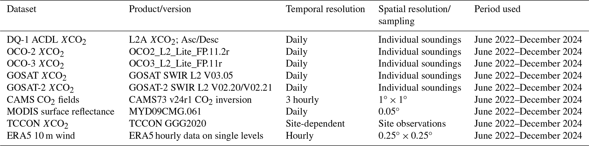
The satellite XCO₂ products, CAMS CO₂ data, MODIS surface reflectance data, ERA5 10 m wind data, and TCCON ground-based observations used in this study are summarized in Table 1. This section introduces these datasets in relation to the active–passive XCO₂ consistency assessment, while the detailed processing and comparison methods are described in Sect. 2.2.

2.1.1 DQ-1 ACDL L2A XCO₂ product

The DQ-1/ACDL L2A XCO₂ product is used as the active lidar dataset in this study. The retrieval algorithm, error characterization, and quality-control procedure of the product are described in detail by Han et al. (2025). Ascending (Asc) and descending (Desc) observations correspond to daytime and nighttime overpasses, respectively, and are processed separately. Quality filtering retains only valid retrievals with QAflag=1 or 5, where QAflag=1 denotes a normal retrieval and QAflag=5 denotes a normal retrieval with a high signal-to-noise ratio. Because the released ACDL L2A product does not provide a dedicated flag for missing hard targets, QAflag=3, which denotes abnormal retrievals associated with low echo intensity, is used here only as an operational proxy for insufficient return signal rather than as a direct identification of missing hard targets. During June 2022–December 2024, QAflag=3 accounted for 15.60 % of the examined L2A records, with monthly fractions ranging from 13.80 %–17.68 % and no clear recurring seasonal cycle. These records lack valid footprint geolocation in the released L2A product, preventing a robust assessment of their geographical distribution.

The main variables used in this study include XCO₂, XCO₂_uncertainty, Hour, Day_Flag, SurfacePressure, PressureLevel, and the vertical weighting function (WF). Here, XCO₂ represents the column-averaged CO₂ dry-air mole fraction for each valid ACDL observation, and XCO₂_uncertainty denotes the retrieval uncertainty reported in the product. Hour and Day_Flag are used to determine the observation time and day–night condition. SurfacePressure, PressureLevel, and WF characterize the effective ACDL integration column and its vertical sensitivity, and are used in the correction for XCO₂ column-definition differences in Sect. 2.2.3. Because DQ-1 active lidar observations do not rely on solar illumination, daytime DQ-1 samples are used for the active–passive consistency assessment with passive satellite products, whereas nighttime DQ-1 samples are analyzed separately for the external model-reference diagnosis described in Sect. 2.2.7.

2.1.2 Passive satellite XCO₂ products

To evaluate the consistency between DQ-1 ACDL XCO₂ and passive NIR/SWIR satellite XCO₂ products, we use XCO₂ products from OCO-2, OCO-3, GOSAT, and GOSAT-2 as comparison datasets. These products mainly retrieve XCO₂ from solar-reflected near-infrared and shortwave-infrared absorption spectra; therefore, the observations generally correspond to daytime clear-sky or near-clear-sky conditions.

OCO-2 and OCO-3 are NASA Orbiting Carbon Observatory missions designed to retrieve XCO₂ from reflected solar spectra using three-channel high-resolution grating spectrometers and full-physics retrieval algorithms (Crisp et al., 2017; Eldering et al., 2017; O'Dell et al., 2018; Taylor et al., 2023). GOSAT and GOSAT-2 carry the Thermal And Near-infrared Sensor for carbon Observation Fourier Transform Spectrometer (TANSO-FTS) and its successor TANSO-FTS-2, respectively. Their instrument characteristics, retrieval algorithms, and XCO₂ products have been described in previous studies (Kuze et al., 2009, 2016; Noël et al., 2021, 2022; Suto et al., 2021; Yoshida et al., 2023). For GOSAT-2, the official land- and ocean-specific empirical bias corrections were applied to the individual XCO₂ retrievals following the V02.20 and V02.21 release notes (NIES GOSAT-2 Project, 2026a, b). The official correction coefficients were derived using TCCON GGG2020 as the reference. GOSAT-2 V02.20 was used through February 2024 and V02.21 from March 2024 onward. The empirical bias correction was applied to each quality-controlled individual retrieval before daily 2° aggregation and collocation, whereas the CAMS-based column-definition correction was subsequently applied to the collocated samples. The passive satellite products are provided as individual soundings and provide the XCO₂ observations for comparison with DQ-1. The corresponding quality-control criteria are summarized in Table 2, and the spatiotemporal collocation and column-definition correction are described in Sects. 2.2.2 and 2.2.3. Although all products report XCO₂, their effective column definitions are not identical because the passive products use product-specific prior profiles, pressure weights, and column averaging kernels, whereas DQ-1 ACDL uses its weighting function and effective pressure layers. These differences are accounted for in Sect. 2.2.3.

2.1.3 CAMS CO₂ profiles and column-averaged XCO₂ fields

We use the Copernicus Atmosphere Monitoring Service (CAMS) global greenhouse gas inversion CO₂ product as an external model reference field. The CAMS CO₂ inversion product used here is constrained by surface air-sample observations and generated by the PYVAR atmospheric inversion system, which is based on the LMDZ offline global atmospheric transport model. The product provides surface fluxes, model-level CO₂ dry-air mole fractions, and column-averaged XCO₂, among other variables (Chevallier et al., 2005, 2010).

CAMS is used in three main ways in this study. First, CAMS column-averaged XCO₂ is used to evaluate the spatial homogeneity and short-term temporal coherence within each 2° candidate grid cell, thereby identifying background regions that are more suitable for inter-satellite comparison. Second, CAMS model-level CO₂ profiles are used as a common external profile and are passed through the observation operators of different satellites to construct CAMS-derived XCO₂ values consistent with each satellite's column definition. This allows us to estimate the theoretical differences caused by differences in vertical sensitivity and effective column definition. Third, for nighttime DQ-1 observations, CAMS-derived XCO₂ is used as an external model reference to evaluate the consistency between nighttime DQ-1 XCO₂ and the model reference field. Throughout this study, TCCON is used as the ground-based observational reference for daytime validation, whereas CAMS is used as a model-based common reference for comparison-region selection, column-definition harmonization, and diagnostic analyses. CAMS is not treated as observational truth. The specific uses of CAMS are described in Sects. 2.2.1, 2.2.3, and 2.2.7.

2.1.4 MODIS Band 6 shortwave-infrared surface reflectance

To examine the potential influence of shortwave-infrared surface reflectance on the differences between DQ-1 and passive satellite XCO₂, we use the Aqua MODIS MYD09CMG.061 daily surface reflectance product. MYD09CMG is a Level-3 Climate Modeling Grid product that provides atmospherically corrected surface reflectance in the visible, near-infrared, and shortwave-infrared spectral regions (Vermote et al., 1997, 2002; Vermote and Kotchenova, 2008).

We select MYD09CMG Band 6 (1628–1652 nm) as a proxy for surface reflectance near the 1.6 µm CO₂ absorption region. This band is not the actual retrieval channel of any of the XCO₂ sensors and is not used for any XCO₂ correction. Instead, it is used only as a common indicator of surface optical conditions to diagnose whether the bias and RMSE between DQ-1 and passive satellite XCO₂ vary systematically with surface reflectance. The MODIS quality filtering, spatial aggregation, and reflectance binning methods are described in Sect. 2.2.4.

2.1.5 ERA5 10 m wind

To examine the potential influence of ocean surface conditions on the differences between DQ-1 and passive satellite XCO₂, we use hourly 10 m wind data from the fifth-generation European Centre for Medium-Range Weather Forecasts (ECMWF) reanalysis, ERA5 (Hersbach et al., 2020). ERA5 provides globally complete atmospheric fields on a regular 0.25°×0.25° latitude–longitude grid. We use the 10 m zonal and meridional wind components (u10 and v10) to derive 10 m wind speed. Over the ocean, near-surface wind influences sea-surface roughness and thus the sun-glint reflectance relevant to passive NIR/SWIR observations (Nelson et al., 2020). ERA5 10 m wind speed is therefore used as an auxiliary indicator of ocean surface conditions to diagnose whether the DQ-1–OCO-2/OCO-3 bias and RMSE vary systematically with surface wind conditions.

2.1.6 TCCON ground-based XCO₂ observations

We use the Total Carbon Column Observing Network (TCCON) GGG2020 data product as a ground-based validation reference. TCCON retrieves the column-averaged dry-air mole fraction of CO₂ from ground-based Fourier transform spectrometer measurements of solar near-infrared absorption spectra, and it is widely used for the validation of OCO-2/OCO-3, GOSAT/GOSAT-2, and other satellite XCO₂ products (Noël et al., 2022; Taylor et al., 2023; Wunch et al., 2010, 2011).

Only TCCON XCO₂ observations that pass the official quality control are used in this study. Because TCCON relies on direct solar spectra, it is mainly used for the validation of daytime DQ-1 observations and passive satellite XCO₂ products. The satellite–TCCON collocations analyzed in this study were not used to derive any additional bias correction. The TCCON sites and valid observation periods used for validation are listed in Table A2. The satellite–TCCON spatiotemporal matching method is described in Sect. 2.2.6.

Table 1 Overview of the datasets used in this study.

2.2 Methods

To reduce the influence of real atmospheric gradients, observation-time differences, and uneven sensor sampling on inter-satellite XCO₂ comparisons, we first identify coherent and well-sampled comparison regions on a global 2°×2° grid. Candidate grid cells are required to satisfy three conditions: weak spatial gradients in the CAMS background field within the grid cell, high consistency in short-term temporal variations among subgrid cells, and sufficient effective multi-sensor observational coverage. For this purpose, we construct a CAMS-based spatiotemporal coherence score and a satellite sampling availability score, and then determine the final comparison regions using a combined score. Based on these selected regions, all active–passive satellite comparisons are based on daily samples aggregated within selected 2° comparison grid cells, rather than direct footprint-level or point-by-point matching.

2.2.1 Selection of coherent and well-sampled comparison regions

(1) CAMS-based spatiotemporal coherence score

CAMS XCO₂ is first averaged to daily fields and then used to evaluate the internal consistency of each 2°×2° grid cell. Because the native horizontal resolution of CAMS is 1°×1°, each 2° grid cell contains up to four 1° subgrid cells. For day d and 2° grid cell g, the spatial dispersion of subgrid XCO₂ relative to the 2° grid-cell mean is defined as:

$$\begin{array}{}\text{(1)}& {\mathit{\sigma }}_{\text{sp}}(d,g)={\left[{\displaystyle \frac{\mathrm{1}}{N_{\mathrm{g}}}}\sum _{k=\mathrm{1}}^{N_{\mathrm{g}}}(X_{d,k}-{\stackrel{\mathrm{‾}}{X}}_d(g){)}^{\mathrm{2}}\right]}^{\mathrm{1}/\mathrm{2}}\end{array}$$

where X_d,k denotes the daily mean XCO₂ for the 1° subgrid cell k on day d, ${\stackrel{\mathrm{‾}}{X}}_d\left(g\right)$ is the daily mean XCO₂ of the corresponding 2° grid cell, and N_g is the number of valid subgrid cells. The quantity σ_sp(d,g) represents the subgrid heterogeneity within a 2° grid cell on a given day. Over the study period, the median and 95th percentile of σ_sp(d,g) are denoted as σ_sp,med(g) and σ_sp,95(g), respectively, and are used to characterize spatial heterogeneity under typical and highly dispersed conditions.

To evaluate whether short-term temporal variations are consistent among the 1° subgrid cells within the same 2° grid cell, a 30 d moving-mean background is removed from the daily XCO₂ time series of each subgrid cell to obtain a high-pass anomaly series:

$$\begin{array}{}\text{(2)}& X_{d,k}^{\prime }=X_{d,k}-{\stackrel{\mathrm{̃}}{X}}_{d,k}^{\mathrm{30}}\end{array}$$

where $X_{d,k}^{\prime }$ denotes the high-pass XCO₂ anomaly for kth subgrid cell on day d, and ${\stackrel{\mathrm{̃}}{X}}_{d,k}^{\mathrm{30}}$ denotes the 30 d moving-mean background. Let P be the set of pairwise combinations of 1° subgrid cells within the 2° grid cell g. The temporal consistency index is then defined as:

$$\begin{array}{}\text{(3)}& \text{TCI}\left(g\right)={\displaystyle \frac{\mathrm{1}}{N_P}}\sum _{(p,q)\in P}{\text{corr}}_d(X_{d,p}^{\prime },X_{d,q}^{\prime })\end{array}$$

where corr_d denotes the Pearson correlation coefficient calculated from the daily anomaly series. A higher TCI(g) indicates more consistent short-term XCO₂ temporal variations within the grid cell.

To describe whether the relative differences among subgrid cells remain stable over time, the stability of internal spatial differences is defined as:

$$\begin{array}{}\text{(4)}& \text{SDI}\left(g\right)={\displaystyle \frac{\mathrm{1}}{N_P}}\sum _{(p,q)\in P}{\text{std}}_d(X_{d,p}-X_{d,q})\end{array}$$

where std_d denotes the standard deviation calculated along the time dimension. Grid cells with fewer than 60 valid days are excluded from the scoring procedure to avoid unstable correlation and percentile statistics caused by overly short time series.

The quantities σ_sp,med, σ_sp,95, TCI, and SDI are then normalized using the 5th and 95th percentiles across all valid 2° grid cells and clipped to the range 0–1. Lower values of σ_sp,med, σ_sp,95, and SDI indicate higher coherence; therefore, their normalized values are reversed. In contrast, higher TCI values indicate stronger temporal consistency. The final CAMS-based spatiotemporal coherence score is defined as:

$$\begin{array}{}\text{(5)}& \begin{array}{rl}& S_{\text{CAMS}}\left(g\right)=\\ & {\displaystyle \frac{H_{\text{sp,med}}\left(g\right)+H_{\text{sp},\mathrm{95}}\left(g\right)+C_{\text{TCI}}\left(g\right)+H_{\text{SDI}}\left(g\right)}{\mathrm{4}}}\end{array}\end{array}$$

where H_sp,med(g), H_sp,95(g), C_TCI(g), and H_SDI(g) are the four normalized components. A higher S_CAMS(g) indicates that the CAMS XCO₂ field within the 2° grid cell has lower spatial dispersion, more stable internal spatial differences, and more coherent short-term temporal variability.

(2) Multi-satellite sampling availability score

To ensure stable multi-satellite observational coverage in the candidate 2° grid cells, we construct a satellite sampling availability score. For each satellite, daily XCO₂ observations after quality control are first assigned to the same 2° grid according to the latitude and longitude of the observation center. Following the grid-based spatial-coverage method of Han et al. (2024) and the path-length-based definition of valid gridded observations described by Han et al. (2025), we do not use the raw number of observations as the only criterion for determining valid gridded observations. Instead, for each sensor, day, and grid cell, we calculate the along-track sampling length by accumulating the great-circle distances between adjacent valid observation centers along the same orbit track. For each sensor and day, only grid cells with an accumulated sampling length greater than or equal to half of the diagonal length of the local 2° grid cell are counted as one valid observation. DQ-1 Asc and Desc are counted separately, and DQ-1 Total (Asc+Desc) is calculated as the direct sum of the two counts. The number of valid observations is then accumulated over the study period and normalized to the range 0–1 using the 95th percentile among grid cells with positive values, yielding the satellite sampling availability score.

On this basis, the mean sampling availability of the main sensors is calculated by averaging A_s(g):

$$\begin{array}{}\text{(6)}& A_{\text{mean}}\left(g\right)={\displaystyle \frac{\mathrm{1}}{n_s}}\sum _{s=\mathrm{1}}^{n_s}{A}_{\mathrm{s}}\left(g\right)\end{array}$$

where A_mean(g) represents the overall sampling sufficiency of grid cell g, A_s(g) is the normalized sampling-availability score derived from the accumulated number of valid observations for sensor s, and n_s is the number of sensors included in the main score (n_s=5). These sensors include daytime DQ-1, OCO-2, OCO-3, GOSAT, and GOSAT-2.

To avoid high scores being dominated by a single sensor, we further calculate the sampling evenness among sensors:

$$\begin{array}{}\text{(7)}& {\displaystyle }& {\displaystyle }{E}_{\text{sensor}}\left(g\right)=-{\displaystyle \frac{{\sum }_{s=\mathrm{1}}^{n_s}{p}_s\left(g\right)\ln p_s\left(g\right)}{\ln n_s}}\text{(8)}& {\displaystyle }& {\displaystyle }{p}_s\left(g\right)={\displaystyle \frac{H_s\left(g\right)}{{\sum }_{s=\mathrm{1}}^{n_s}{H}_s\left(g\right)}}\end{array}$$

where E_sensor(g) is the Shannon evenness calculated from the sensor contribution fractions. It is higher when the contributions from multiple sensors are more balanced and lower when the valid observations are dominated by a single sensor. Here, p_s(g) denotes the fraction of valid observations contributed by sensor s in grid cell g, calculated as the accumulated number of valid observations H_s(g) of sensor s divided by the total accumulated valid observation days from all sensors.

The multi-sensor same-day sampling support is defined as:

$$\begin{array}{}\text{(9)}& C_{\text{multi}}\left(g\right)=min\left[{\displaystyle \frac{D_{\text{multi}}\left(g\right)}{P_{\mathrm{95}}(D_{\text{multi}}>\mathrm{0})}},\mathrm{1}\right]\end{array}$$

where C_multi(g) represents the same-day multi-sensor observation support for grid cell g. It is obtained by normalizing D_multi(g), the accumulated number of days on which at least two main sensors satisfy the valid-observation condition on the same day, using its 95th percentile.

The final satellite sampling availability score is defined as:

$$\begin{array}{}\text{(10)}& S_{\text{SAT}}\left(g\right)={\displaystyle \frac{A_{\text{mean}}\left(g\right)+E_{\text{sensor}}\left(g\right)+C_{\text{multi}}\left(g\right)}{\mathrm{3}}}\end{array}$$

where S_SAT(g) accounts for mean sampling sufficiency, sampling evenness among sensors, and same-day multi-sensor observation support.

(3) Final score and selection of comparison regions

The final comparison-region score is determined jointly by the CAMS-based spatiotemporal coherence score and the satellite sampling availability score. To ensure both background-field coherence and sufficient multi-satellite sampling, we define the final score as the geometric mean of the two component scores:

$$\begin{array}{}\text{(11)}& S_{\text{final}}\left(g\right)=\sqrt{S_{\text{CAMS}}\left(g\right)S_{\text{SAT}}\left(g\right)}\end{array}$$

where S_final(g) denotes the final score for grid cell g. For the final selection, the 90th percentile of S_final is calculated separately for land and ocean grid cells. The 2° grid cells with S_final greater than or equal to the corresponding land or ocean threshold are retained as the final comparison regions. The P90 threshold was adopted as a conservative reference criterion. It prioritizes grid cells with relatively high background-field coherence and sufficient multi-satellite sampling. This choice was not intended to imply that P90 is an empirically optimized threshold. To test the sensitivity to this choice, we repeated the inter-satellite comparisons using P80 and P70 thresholds. These thresholds retain approximately the upper 20 % and 30 % of eligible land and ocean grid cells, respectively. All other processing and collocation procedures were kept unchanged. The sensitivity cases and results are presented in Appendix A2.

2.2.2 Inter-satellite spatiotemporal collocation and sample selection

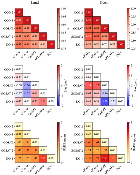
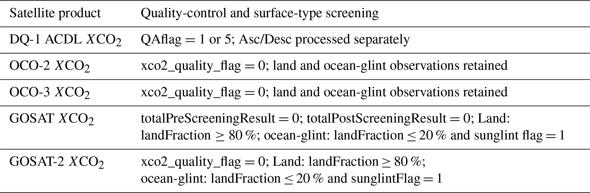
The quality-control criteria applied to each satellite XCO₂ product are listed in Table 2. Inter-satellite comparisons are based on daily samples aggregated within selected 2° comparison grid cells, rather than on matching individual soundings or footprints. After quality control, valid XCO₂ observations are assigned to the selected 2° comparison grid cells according to the latitude and longitude of their observation centers. For each date and selected grid cell, the daily XCO₂ and mean observation time are calculated using simple arithmetic averaging over all valid observations within the grid cell. A sample pair is considered a candidate pair only when the two products fall within the same selected 2° comparison grid cell on the same date and both satisfy the valid-observation criterion defined in Sect. 2.2.1. Candidate pairs are retained as final paired samples only if the difference between their daily mean observation times does not exceed 4 h. For the pairwise statistics shown in Fig. 4 and Table S3 in the Supplement, bias is defined as XCO₂(y-axis product) − XCO₂(x-axis product).

The 2° aggregation was chosen as a common analysis scale for sensors with different footprint sizes and sampling densities. It is also consistent with the CAMS-based coherence analysis, because each 2° grid cell contains up to four native 1° CAMS grid cells. A finer 1° grid would therefore not preserve the same within-cell coherence assessment. The 4 h temporal window was selected to balance temporal representativeness with the availability of valid collocations among satellites with different sampling characteristics. A comparable 4 h criterion has also been used in direct OCO-2/OCO-3 XCO₂ comparisons (Taylor et al., 2023). We therefore retained the 2° grid and tested temporal windows of 3, 2, and 1 h while keeping the P90 spatial criterion fixed. The sensitivity cases and results are presented in Appendix A2. Unless otherwise stated, the inter-satellite comparison results presented in the main text are based on the Main case, which uses the P90 spatial-selection threshold and a maximum temporal difference of 4 h.

Table 2 Quality-control criteria for the satellite XCO₂ products.

2.2.3 Correction for XCO₂ column-definition differences among satellites

The active and passive satellite XCO₂ products do not necessarily share the same effective column definition because they differ in prior profiles, pressure weighting functions, column averaging kernels, and vertical sensitivities. If the retrieved XCO₂ values are compared directly, part of the difference may arise from differences in the observation operators, rather than from real atmospheric CO₂ differences. To reduce this effect, we use CAMS 3 hourly CO₂ profiles as a common external reference profile and apply the observation operator of each satellite to these profiles to estimate the theoretical difference caused by XCO₂ column-definition differences.

For a given satellite s, the CAMS-derived XCO₂ under the column definition of that satellite is expressed as:

$$\begin{array}{}\text{(12)}& X_s^{\text{CAMS}}={\mathcal{H}}_s\left(c^{\text{CAMS}}\right)\end{array}$$

where ℋ_s is the XCO₂ observation operator of satellite s, and c^CAMS is the CAMS CO₂ profile.

For the passive products from OCO-2, OCO-3, GOSAT, and GOSAT-2, c^CAMS is interpolated to the pressure levels of the corresponding product and then used together with the product-specific pressure weights and column averaging kernels to calculate XCO₂:

$$\begin{array}{}\text{(13)}& X_s^{\text{CAMS}}=X_s^a+\sum _{k=\mathrm{1}}^{n_s}{w}_{s,k}{A}_{s,k}\left[c_k^{\text{CAMS}}-c_{s,k}^a\right]\end{array}$$

where $X_s^a$ is the prior XCO₂ of satellite s, w_s,k and A_s,k are the pressure weight and column averaging kernel for layer k, respectively, $c_{s,k}^a$ is the prior CO₂ mixing ratio, and $c_k^{\text{CAMS}}$ is the CAMS CO₂ mixing ratio interpolated to the corresponding pressure level p_s,k.

For DQ-1/ACDL, the active lidar retrieval uses the weighting function (WF) to describe vertical sensitivity. The CAMS profile is therefore integrated using the DQ-1 WF and the effective pressure thickness:

$$\begin{array}{}\text{(14)}& X_{\text{DQ1}}^{\text{CAMS}}={\displaystyle \frac{{\sum }_{k=\mathrm{1}}^m{c}^{\text{CAMS}}\left(p_k\right){\text{WF}}_k\mathrm{\Delta }{p}_k}{{\sum }_{k=\mathrm{1}}^m{\text{WF}}_k\mathrm{\Delta }{p}_k}}\end{array}$$

where WF_k is the DQ-1 weighting function for layer k, and Δp_k is the effective pressure thickness of that layer.

For each satellite sample pair satisfying the spatiotemporal collocation criteria, s denote the product under evaluation and r denote the reference product. The theoretical XCO₂ column-definition difference caused by differences in the observation operators is then defined as:

$$\begin{array}{}\text{(15)}& \mathrm{\Delta }{X}_{r-s}^{\text{def}}=X_r^{\text{CAMS}}-X_s^{\text{CAMS}}\end{array}$$

This definition difference is subsequently added to the observed XCO₂ of the product under evaluation, thereby converting it to the XCO₂ definition of the reference product:

$$\begin{array}{}\text{(16)}& X_{s\to r}^{\text{corr}}=X_s^{\text{obs}}+\mathrm{\Delta }{X}_{r-s}^{\text{def}}\end{array}$$

This correction only accounts for the theoretical difference produced when the same CO₂ profile is represented under different satellite column definitions. CAMS is used only to estimate column-definition differences and is not treated as a truth reference for correcting satellite biases. The term $\mathrm{\Delta }{X}_{r-s}^{\text{def}}$ reflects only differences in the observation operators and effective column definitions. The differences after this correction may still include contributions from instrumental errors, retrieval errors, spatiotemporal sampling differences, and uncertainties in the CAMS CO₂ profiles.

2.2.4 Diagnosis of DQ-1–OCO-2/OCO-3 XCO₂ residuals using MODIS surface reflectance

The MODIS MYD09CMG Band 6 shortwave-infrared surface reflectance is used only to diagnose the influence of surface optical conditions on the DQ-1–OCO-2/OCO-3 XCO₂ differences. It is not used for any XCO₂ correction. For the DQ-1–OCO-2 and DQ-1–OCO-3 paired samples that have passed the spatiotemporal collocation and XCO₂ column-definition correction procedures, we extract the mean MODIS Band 6 reflectance within the same selected 2° comparison grid cell on the same day. Only samples with reflectance values between 0 and 1 and with at least 10 valid MODIS subpixels are retained, to reduce the influence of anomalous reflectance values on the statistics.

For each selected 2° grid cell, we then calculate the mean reflectance, mean bias, and RMSE. The RMSE is defined as the square root of the mean squared residuals of all valid paired samples within the same grid cell. Based on these 2° grid-cell statistics, the samples are further binned according to the grid-cell mean reflectance. A reflectance bin width of 0.05 is used for all samples and land samples, whereas a bin width of 0.02 is used for ocean samples to account for the smaller range of shortwave-infrared reflectance over the ocean. Statistics are calculated for a reflectance bin only when it contains at least 10 valid 2° grid cells. Within each reflectance bin, bias and RMSE are reported as the arithmetic means of the grid-cell mean bias values and grid-cell RMSE values, respectively. The error bars indicate the standard deviations of the corresponding 2° grid-cell statistics within the same reflectance bin. The linear least-squares fits and Pearson correlation coefficients shown in Figs. 6 and 7 are calculated from the displayed reflectance-bin means.

2.2.5 Diagnosis of oceanic residuals using ERA5 10 m wind speed

To further examine the potential influence of ocean surface conditions on the DQ-1–OCO-2/OCO-3 differences, ERA5 10 m zonal and meridional wind components (u10 and v10) are collocated in space and time with the oceanic paired samples and used to derive 10 m wind speed. For each selected 2° ocean grid cell, the mean wind speed, mean bias, and RMSE are calculated, and the resulting grid-cell statistics are further grouped into wind-speed bins. The mean bias and RMSE within each bin are used to assess whether the active–passive XCO₂ differences vary systematically with near-surface wind conditions. Wind-speed bins have a width of 1 m s⁻¹. Linear least-squares fits and Pearson correlation coefficients are calculated separately for the individual 2° grid-cell statistics and for the wind-speed-bin means shown in Fig. S6 in the Supplement.

2.2.6 Validation with TCCON observations

TCCON is used as a common ground-based reference for satellite XCO₂ validation. Following the validation approach for DQ-1/ACDL described by Han et al. (2025), we construct a 1°×1° spatial matching window centered on each TCCON site and extract quality-controlled TCCON XCO₂ observations within ±0.5 h of the satellite overpass time. If multiple TCCON observations are available within the matching window, their median value is used as the reference. For the matched satellite samples, we estimate and correct the definition difference caused by differences in XCO₂ column definition and vertical sensitivity following Sect. 2.2.3. The corrected satellite XCO₂ is then compared with the TCCON reference value, and bias, RMSE, and the Pearson correlation coefficient (R) are calculated. To assess site-to-site variability and the potential influence of uneven collocation numbers across TCCON sites, we additionally calculated site-level validation statistics. The interstation bias was defined as the standard deviation of the mean biases calculated separately for individual TCCON sites, while the site-mean RMSE was defined as the mean of the site-specific RMSE values, with each TCCON site weighted equally. The 95 % confidence intervals of the pooled bias and RMSE were estimated using a TCCON-site cluster bootstrap with 20 000 resamples, in which contributing sites were sampled with replacement and all collocations from each selected site were retained together.

2.2.7 Comparison of nighttime DQ-1 XCO₂ with CAMS-derived XCO₂

Because passive shortwave-infrared satellites and TCCON do not provide nighttime XCO₂ observations, CAMS CO₂ is used as an external model reference field for evaluating nighttime DQ-1 XCO₂. We first select nighttime DQ-1 L2A observations that pass quality control, are located within the selected comparison regions, and satisfy the valid-observation criterion defined in Sect. 2.2.1. These observations are then aggregated by date and selected 2° comparison grid cell. XCO₂, WF, SurfacePressure, and Hour are averaged arithmetically over the valid observations within each grid cell.

The nearest CAMS CO₂ profile is then matched according to the mean DQ-1 observation time. Using the aggregated WF and SurfacePressure, the CAMS profile is converted to XCO₂ under the DQ-1 column definition. The resulting CAMS-derived XCO₂ is finally paired with nighttime DQ-1 XCO₂, and bias, RMSE, and the Pearson correlation coefficient are calculated. The difference is defined as DQ-1 minus CAMS-derived XCO₂. This comparison is used to evaluate the consistency and stability of nighttime DQ-1 relative to an external model reference field, and should not be interpreted as an independent absolute validation against observations. As an additional diagnostic of possible day–night retrieval differences, we also compare the zonal-mean daytime–nighttime XCO₂ difference in DQ-1 with the corresponding difference in CAMS-derived XCO₂ under the DQ-1 column definition. Because direct spatial overlap between daytime and nighttime ACDL ground tracks is sparse, this analysis is performed at the zonal-mean level rather than using strict point-by-point daytime–nighttime collocation.

3 Results

3.1 Coherent and well-sampled comparison regions

Figure 2 shows the CAMS-based spatiotemporal coherence score (CAMS score), the satellite sampling availability score (SAT score), the final score, and the selected 2° comparison grid cells. The CAMS score is generally higher over open-ocean regions and areas with weak XCO₂ background gradients, including parts of the low- and middle-latitude oceans and the open Southern Hemisphere oceans. In contrast, lower CAMS scores occur over land–ocean transition zones, strong source–sink regions, complex-terrain areas, and land regions with strong XCO₂ spatial gradients, indicating larger subregional XCO₂ variability in these areas. The spatial distribution of the SAT score is mainly controlled by multi-sensor sampling availability. High SAT scores are concentrated in regions with relatively frequent repeated observations from multiple satellites, including North Africa–Arabia, Europe–Central Asia, East Asia, Australia, and several oceanic sampling bands. In contrast, lower SAT scores occur at high latitudes, in regions strongly affected by cloud and aerosol filtering, and over sparsely sampled ocean areas.

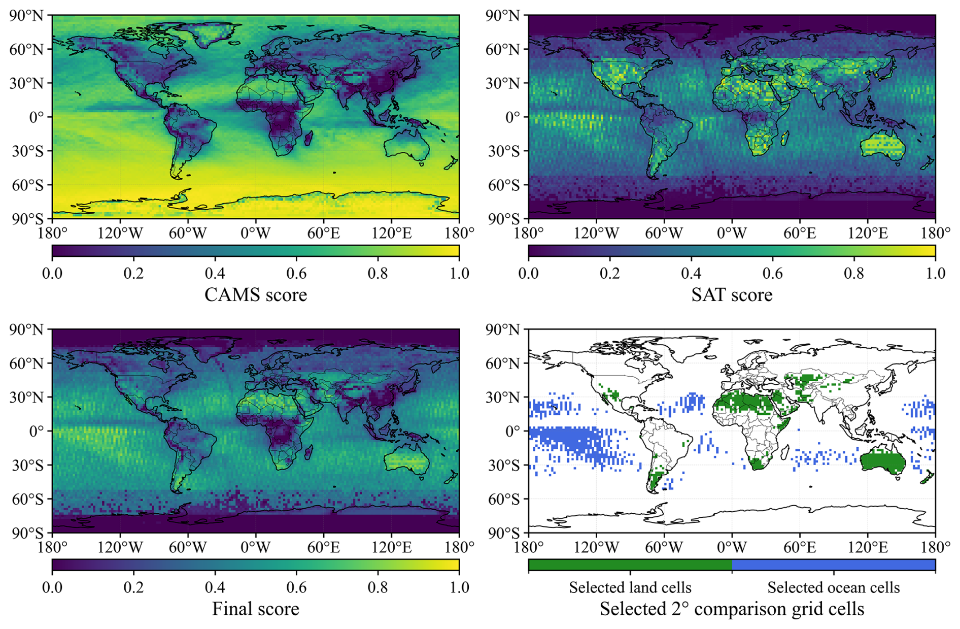
Figure 2 Spatial distributions of the CAMS-based coherence score, satellite sampling availability score, final score, and selected 2° comparison grid cells.

The final score jointly reflects background-field coherence and multi-satellite sampling availability. Based on this score, we selected 1297 2° comparison grid cells, including 540 land grid cells and 757 ocean grid cells. The selected land regions are mainly distributed over North Africa–Arabia, Central Asia, Europe, Australia, and parts of North America, whereas the selected ocean regions are mainly located over open oceans at low and middle latitudes. These selected regions define the spatial domain for the subsequent daily paired comparisons between active DQ-1 and passive XCO₂ products, and provide a set of regional samples with relatively stable background conditions and sufficient sampling support for the inter-satellite consistency assessment.

3.2 Validation of satellite XCO₂ products against TCCON observations

We first compare the five satellite XCO₂ products with TCCON observations to assess their overall agreement with a common ground-based reference. Figure 3 shows that OCO-2 and OCO-3 have the strongest agreement with TCCON, with correlation coefficients of R=0.95 and 0.94, mean biases of −0.18 and 0.08 ppm, and RMSE values of 1.09 and 1.12 ppm, respectively. These results indicate small systematic biases and random scatter for the OCO products, consistent with the validation results for OCO-2 and OCO-3 reported by Taylor et al. (2023). GOSAT also agrees well with TCCON, with R=0.91, a mean bias of −0.28 ppm, and an RMSE of 1.45 ppm. Overall, OCO-2, OCO-3, and GOSAT show close agreement with TCCON, with absolute mean biases below 0.3 ppm and RMSE values below 1.5 ppm.

For GOSAT-2, the uncorrected XCO₂ product shows a pronounced positive bias relative to TCCON, with R=0.91, a mean bias of 3.56 ppm, and an RMSE of 3.98 ppm (gray symbols in Fig. 3d). Similar positive biases of GOSAT-2 XCO₂ relative to TCCON have also been reported in previous studies (Ji et al., 2024; Yang et al., 2025). After applying the official empirical bias correction to the pixel-level GOSAT-2 XCO₂ data, the mean bias decreases to 0.01 ppm and the RMSE to 1.54 ppm, while R changes only slightly to 0.92 (colored symbols in Fig. 3d). The substantial reductions in bias and RMSE indicate that the pronounced overestimation in the uncorrected product is largely associated with systematic biases addressed by the empirical correction. After correction, GOSAT-2 shows good agreement with TCCON.

The comparison between DQ-1 and TCCON shows that, although the number of valid collocations is smaller than that for the passive satellites, DQ-1 still has R=0.92, a mean bias of 0.21 ppm, and an RMSE of 1.49 ppm. These statistics are comparable to those of GOSAT and empirically corrected GOSAT-2, although the OCO-2 and OCO-3 comparisons show slightly lower RMSE values, indicating that daytime DQ-1 ACDL XCO₂ is consistent with TCCON observations. This result is consistent with the initial validation of ACDL XCO₂ by Han et al. (2025), who reported a near-zero mean bias and an RMSE of about 1.4 ppm. The relatively limited number of DQ-1–TCCON collocations is mainly constrained by the point-sampling geometry of the active lidar observations. Unlike passive sensors with wider swaths or denser sampling, DQ-1/ACDL samples only along its ground track, which reduces the probability of close spatiotemporal coincidence with TCCON sites.

Additional information on the site-level sampling and validation statistics is provided in Tables S1 and S2 in the Supplement. The site-mean RMSE differs from the corresponding overall RMSE by no more than 0.16 ppm across the satellite products, suggesting that the overall RMSE is not strongly affected by the unequal numbers of collocations among TCCON sites. The interstation bias ranges from 0.56–1.40 ppm, with the largest value found for GOSAT, indicating greater site-to-site variability. GOSAT also shows a more concentrated distribution of collocations among a small number of sites. In contrast, the DQ-1 collocations are distributed across 24 TCCON sites, and no individual site accounts for more than 11.4 % of the total, indicating that the DQ-1 validation statistics are not driven by a single site. The 95 % confidence intervals further quantify the uncertainty of the pooled validation statistics. For DQ-1, the bias is 0.21 ppm (95 % CI: $-\mathrm{0.08}-\mathrm{0.48}\mathrm{ppm}$) and the RMSE is 1.49 ppm (95 % CI: 1.25–1.74 ppm). GOSAT shows the widest bias interval ($-\mathrm{0.72}-\mathrm{0.60}\mathrm{ppm}$), consistent with its greater site-to-site variability and more concentrated station sampling.

Overall, the TCCON comparisons show that OCO-2, OCO-3, GOSAT, and empirically corrected GOSAT-2 are in good agreement with the ground-based reference. Daytime DQ-1 ACDL XCO₂ also agrees well with TCCON, providing independent validation of the DQ-1 product and supporting its role as a complement to passive satellite XCO₂ observations.

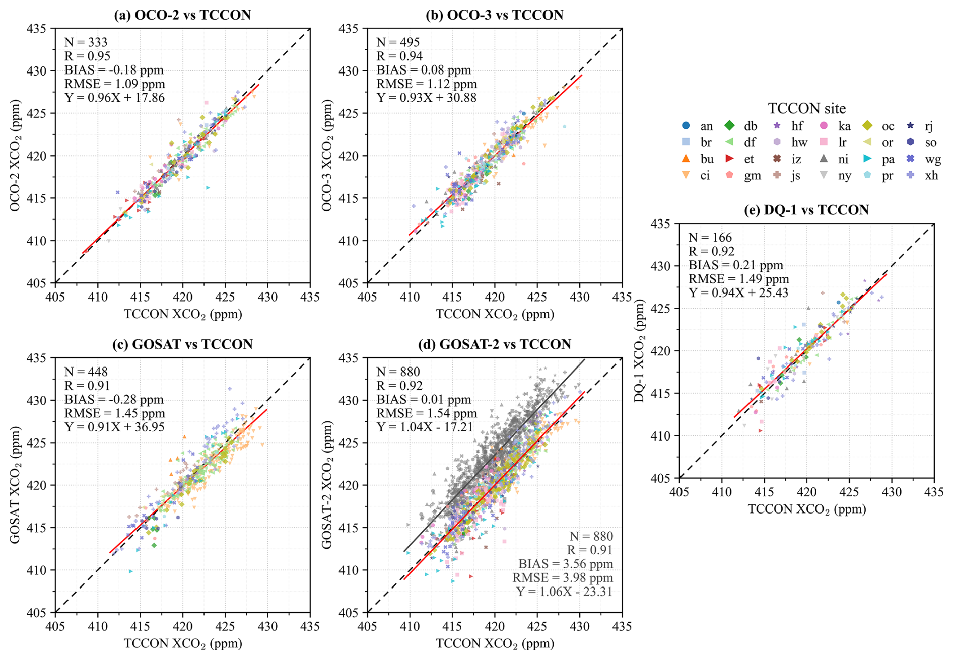
Figure 3 Comparison of satellite XCO₂ products with TCCON observations. (a–e) OCO-2, OCO-3, GOSAT, GOSAT-2, and DQ-1 XCO₂ compared with collocated TCCON XCO₂, respectively. Different colors and symbols denote individual TCCON sites. In panel (d), colored and gray symbols denote empirically bias-corrected and uncorrected GOSAT-2 XCO₂, respectively, with the corresponding linear least-squares fits shown by the red and gray solid lines. Red solid lines in panels (a–c, e) indicate linear least-squares fits, and black dashed lines indicate the 1:1 relationship. The TCCON site abbreviations are defined in Table A2.

3.3 Inter-satellite XCO₂ consistency over the selected comparison regions

Following the independent TCCON evaluation, we next examine the relative consistency among satellite XCO₂ products over the coherent and well-sampled comparison regions. Figure 4 summarizes the pairwise consistency statistics for the five satellite XCO₂ products over the selected comparison regions. Figure S1 in the Supplement shows the spatial distributions of the CAMS-derived column-definition differences, and Table S3 reports the pairwise statistics before and after the column-definition correction. The mean DQ-1-minus-OCO-2, OCO-3, GOSAT, and GOSAT-2 column-definition differences are 0.44, 0.44, 1.30, and 0.49 ppm, respectively. The correction changes the correlation coefficients by no more than 0.01 in most comparisons, while the bias and RMSE can change more noticeably.

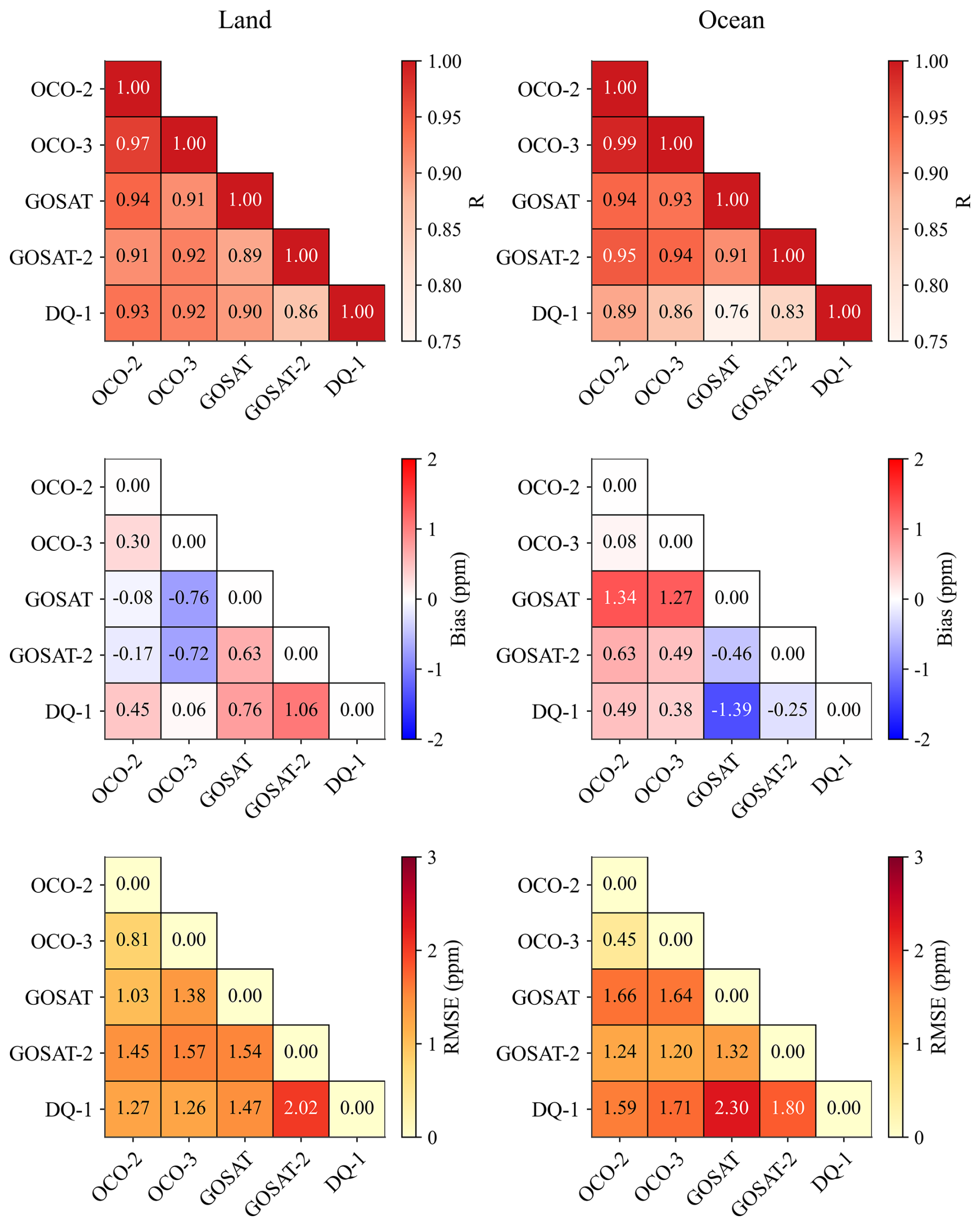
Figure 4 Pairwise consistency metrics for the satellite XCO₂ products over land and ocean in the selected comparison regions. Empirically corrected GOSAT-2 XCO₂ is used in these comparisons. Bias is defined as the y-axis product minus the x-axis product.

The passive satellite products generally show high consistency with one another, with correlation coefficients R mostly around 0.9 for both land and ocean samples. The agreement between OCO-2 and OCO-3 is the strongest, with R=0.97 over land and R=0.99 over ocean, mean biases of −0.30 and −0.08 ppm, and RMSE values of 0.81 and 0.45 ppm, respectively. GOSAT is also broadly consistent with OCO-2 and OCO-3 over land, with $R=\mathrm{0.91}-\mathrm{0.94}$ and RMSE values of 1.03–1.38 ppm. Over ocean, however, GOSAT is approximately 1.3 ppm higher than OCO-2 and OCO-3, indicating that differences among passive satellite XCO₂ products remain over ocean scenes.

The uncorrected GOSAT-2 retrievals show substantially larger differences from the other passive satellite products. After application of the official empirical bias correction, the absolute mean biases across the comparisons with OCO-2, OCO-3, and GOSAT decrease to 0.17–0.72 ppm, with RMSE values of 1.20–1.57 ppm (Table S3). This indicates that the positive differences in the original GOSAT-2 product are largely associated with the systematic component addressed by the empirical correction.

For the comparisons between DQ-1 and the passive satellite products, DQ-1 is generally consistent with OCO-2, OCO-3, and GOSAT. The DQ-1 comparisons with the OCO series show the closest agreement. For land and ocean samples, the DQ-1–OCO-2/OCO-3 comparisons yield $R=\mathrm{0.86}-\mathrm{0.93}$, mean biases of 0.06–0.49 ppm, and RMSE values of 1.26–1.71 ppm. In particular, the mean biases of DQ-1 relative to OCO-2 and OCO-3 are both smaller than 0.5 ppm, indicating that active IPDA XCO₂ from DQ-1 is broadly consistent with the passive OCO products over the selected comparison regions. Compared with GOSAT, DQ-1 also shows high consistency over land, with R=0.90, mean bias=0.76 ppm, and RMSE=1.47 ppm. Over ocean, however, DQ-1 is lower than GOSAT by approximately 1.39 ppm, and the RMSE increases to 2.30 ppm, consistent with the result that GOSAT is higher than the OCO products over ocean.

We further assessed the robustness of the pairwise statistics using different spatial-selection thresholds and temporal-collocation windows (Appendix A2). Using P80 and P70 instead of P90 increased the number of collocations (N) for nearly all satellite pairs because more comparison grid cells were included. However, the corresponding R, bias, and RMSE values remained close to those of the Main case. When the temporal window was narrowed from 4 h to 3, 2, and 1 h, N decreased, especially for satellite pairs with relatively sparse sampling. Despite these changes in sample size, R, bias, and RMSE changed only slightly. These results indicate that the main inter-satellite consistency statistics are robust to reasonable changes in the spatial-selection and temporal-collocation criteria.

Overall, the RMSE values for the DQ-1 comparisons with passive satellite products are higher over ocean than over land, indicating larger scatter in the ocean samples. Because DQ-1 shows the highest consistency with OCO-2 and OCO-3 and these comparisons have the largest matched sample sizes, the subsequent analysis focuses on the spatial distributions of the DQ-1–OCO-2 and DQ-1–OCO-3 residuals and their relationships with MODIS Band 6 surface reflectance.

3.4 Spatial characteristics and diagnosis of DQ-1–OCO-2/OCO-3 XCO₂ differences

3.4.1 Spatial and zonal characteristics of DQ-1–OCO-2/OCO-3 differences

Figure S2 in the Supplement compares the spatial distributions of DQ-1, OCO-2, and OCO-3 XCO₂ over the selected 2° comparison grid cells. Overall, the three products show similar large-scale XCO₂ gradients, with higher values mainly over Northern Hemisphere land and lower values over Southern Hemisphere oceans. The high- and low-XCO₂ patterns in DQ-1 are broadly consistent with those of OCO-2 and OCO-3, indicating that active IPDA and passive NIR/SWIR XCO₂ products have similar spatial structures over the selected comparison regions.

Figure 5 further shows the spatial distributions of the mean DQ-1–OCO-2 and DQ-1–OCO-3 differences, together with the corresponding zonal-mean results. Spatially, most DQ-1–OCO-2 and DQ-1–OCO-3 differences are within approximately ±1 ppm, with no clear global-scale systematic bias. Local positive differences occur mainly over several oceanic sampling bands, Australia, and some low- and middle-latitude land regions, whereas negative differences are scattered over North Africa, Eurasia, and parts of the tropical oceans. Although most grid-cell differences remain within approximately ±1 ppm, several regional features are evident (Fig. 5). Over Australia, the mean DQ-1–OCO-2 and DQ-1–OCO-3 biases are +0.76 and +0.57 ppm, respectively, compared with +0.46 and +0.15 ppm over all selected land grid cells. The tropical Pacific shows a different pattern. For DQ-1–OCO-2, the regional mean bias is +0.58 ppm, slightly higher than the all-ocean value of +0.51 ppm, whereas for DQ-1–OCO-3 the regional mean bias is +0.30 ppm, lower than the corresponding all-ocean value of +0.40 ppm. Thus, an enhanced regional mean bias is not common to both tropical-Pacific comparisons. In contrast, the mean grid-cell RMSE values are 1.27 and 1.26 ppm, respectively, both 0.06 ppm higher than the corresponding all-ocean values of 1.21 and 1.20 ppm (Table S4 in the Supplement). These regional differences are examined further in Sects. 3.4.2 and 3.4.3 using CAMS-derived XCO₂, surface reflectance, and ocean wind-speed diagnostics.

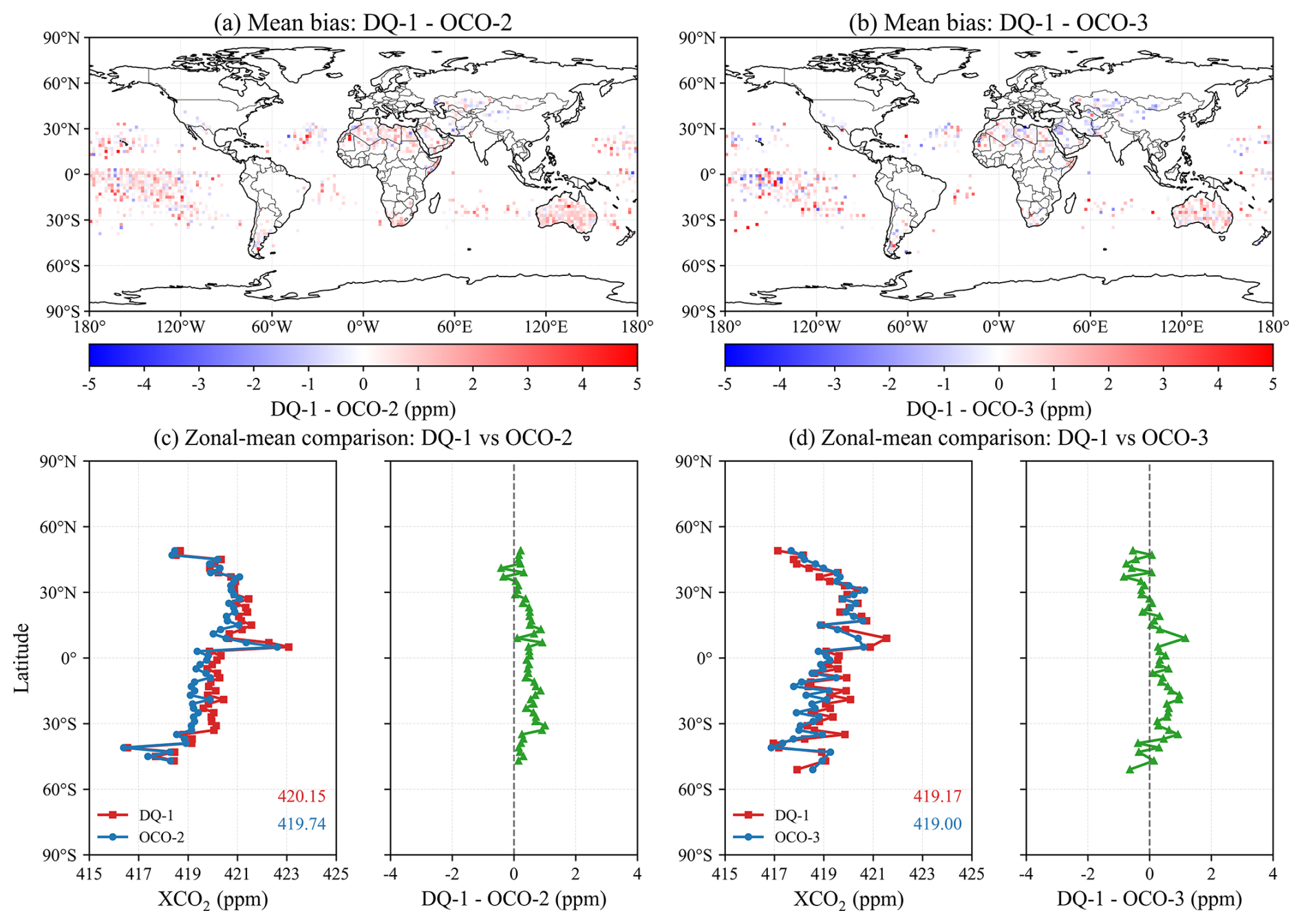
Figure 5 Spatial and zonal differences between DQ-1 and OCO-2/OCO-3 XCO₂ over the selected comparison regions. (a, b) Spatial distributions of the mean DQ-1–OCO-2 and DQ-1–OCO-3 differences, respectively. (c, d) Corresponding zonal-mean XCO₂ values and zonal-mean differences.

The zonal-mean results show that DQ-1 and OCO-2/OCO-3 have broadly consistent meridional XCO₂ variations, with higher values in the Northern Hemisphere mid-latitudes and lower values in the Southern Hemisphere. The zonal-mean values of DQ-1 and OCO-2 are approximately 420.15 and 419.74 ppm, respectively, corresponding to a mean difference of about 0.41 ppm. For the DQ-1–OCO-3 comparison, the corresponding values are approximately 419.17 and 419.00 ppm, with a mean difference of about 0.17 ppm. In most latitude bands, the DQ-1–OCO-2/OCO-3 differences are close to zero, with only small positive or negative deviations in some low- and middle-latitude regions. Overall, DQ-1 is consistent with OCO-2 and OCO-3 in both spatial distribution and meridional structure, indicating that the residual differences between active and passive XCO₂ products are generally small after applying unified filtering, aggregation, collocation, and column-definition correction.

3.4.2 Diagnosis using CAMS-derived XCO₂ as a common diagnostic reference

To further diagnose these regional differences, DQ-1 and OCO-2/OCO-3 were independently compared with CAMS-derived XCO₂ using exactly the same collocated samples (Figs. S3–S4 and Table S5 in the Supplement). Over Australia, DQ-1 shows small positive biases of +0.22 and +0.23 ppm relative to CAMS-derived XCO₂ for the OCO-2 and OCO-3 collocations, respectively, whereas OCO-2 and OCO-3 show negative biases of −0.53 and −0.35 ppm. Thus, the positive DQ-1–OCO differences over Australia are accompanied by opposite-signed departures of DQ-1 and the OCO products from the common CAMS-derived reference. A site-based comparison with TCCON at Darwin and Wollongong provides an independent regional diagnostic and likewise shows a positive DQ-1 bias, although only 10 DQ-1 collocations are available (Fig. S5 in the Supplement). Over the tropical Pacific, the DQ-1–CAMS-derived XCO₂ RMSE values are 1.09 and 1.08 ppm, compared with 0.41 and 0.42 ppm for OCO-2 and OCO-3, respectively. In contrast, over the Sahara, both DQ-1 and the OCO products show RMSE values below 1 ppm relative to CAMS-derived XCO₂, and the contrast between the two products is much smaller than that over the tropical Pacific (Table S5). Over the tropical Pacific, the substantially larger DQ-1 RMSE relative to the common CAMS-derived reference indicates that the enhanced scatter is more evident on the DQ-1 side under these collocated conditions. This differs from Australia, where DQ-1 and the OCO products show opposite-signed mean departures from CAMS. CAMS is used here only as a common diagnostic reference rather than as observational truth; these comparisons therefore help identify relative product behavior but do not uniquely attribute retrieval errors.

3.4.3 Relationships with surface reflectance and ocean wind speed

Figures 6 and 7 show, respectively, the relationships between MODIS Band 6 shortwave-infrared surface reflectance and the bias and RMSE of DQ-1 relative to OCO-2 and OCO-3. Spatially, MODIS reflectance is substantially higher over land than over ocean, especially in arid and semi-arid regions such as North Africa–the Middle East, Australia, and Central Asia, whereas ocean reflectance is generally low and has a narrower range. In contrast, the spatial distribution of bias is more heterogeneous, with positive and negative residuals spatially mixed and no clear correspondence with the reflectance field. The RMSE distribution also does not simply follow the regions of high reflectance. Higher RMSE values occur not only over some high-reflectance land areas and regions with complex surface conditions, but also over parts of the Southern Hemisphere oceans, the tropical Pacific, and coastal regions. Because the ocean residuals cannot be explained consistently by surface reflectance alone, we further examine whether they covary with ERA5 10 m wind speed.

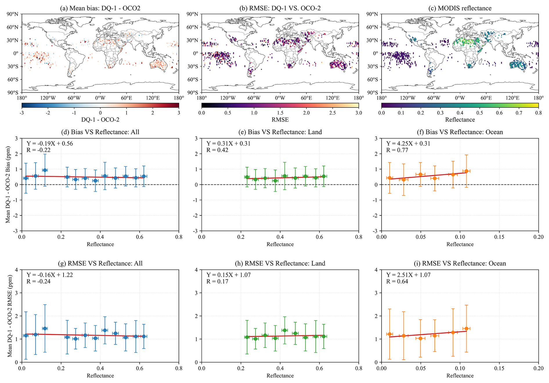
Figure 6 Spatial distributions and reflectance-binned statistics of DQ-1–OCO-2 XCO₂ residuals and MODIS Band 6 surface reflectance. (a–c) Spatial distributions of the mean DQ-1–OCO-2 bias, RMSE, and MODIS Band 6 reflectance, respectively. (d–f) Reflectance-binned mean bias for all, land, and ocean samples, respectively. (g–i) Corresponding reflectance-binned RMSE.

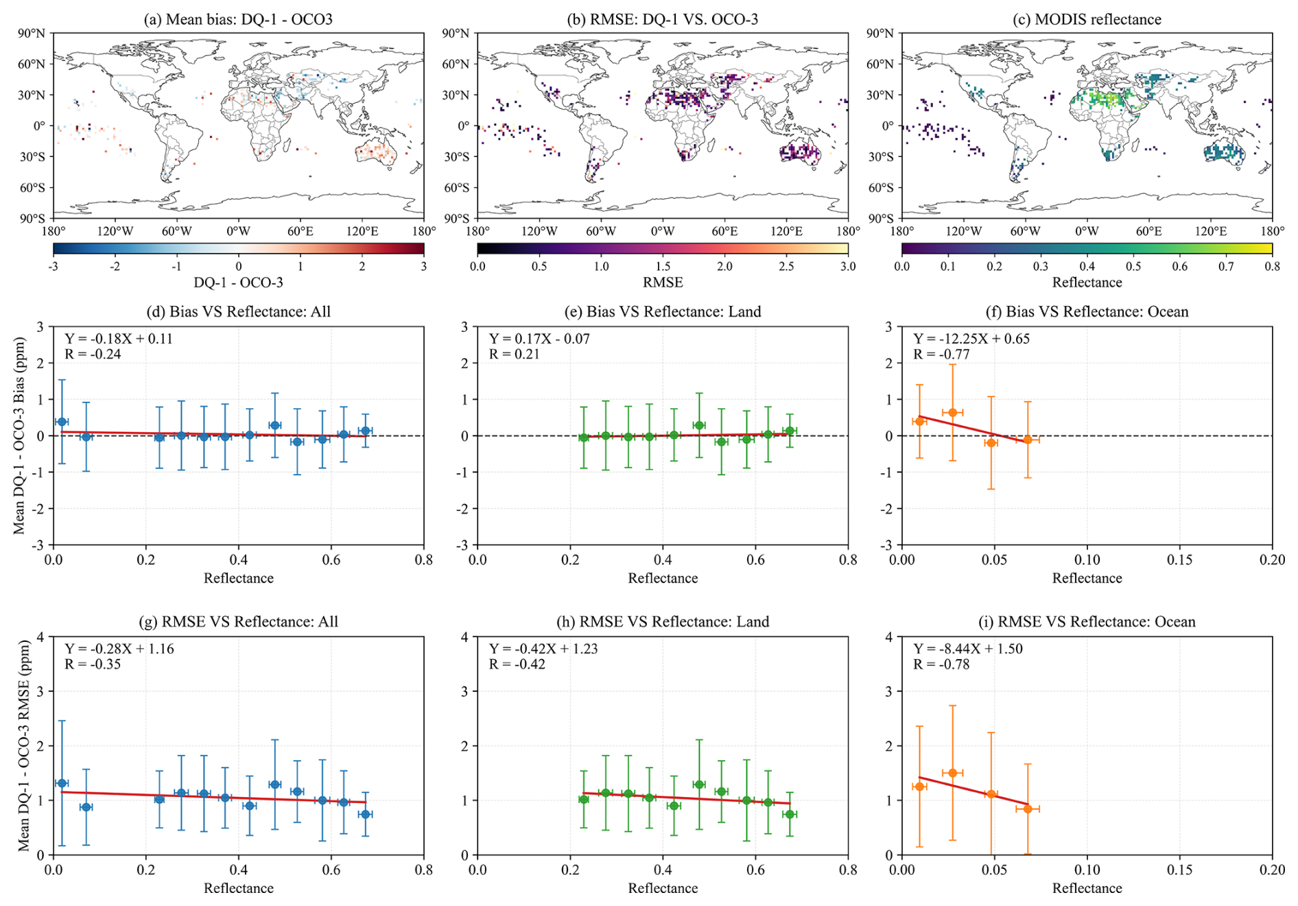
Figure 7 Spatial distributions and reflectance-binned statistics of DQ-1–OCO-3 XCO₂ residuals and MODIS Band 6 surface reflectance. (a–c) Spatial distributions of the mean DQ-1–OCO-3 bias, RMSE, and MODIS Band 6 reflectance, respectively. (d–f) Reflectance-binned mean bias for all, land, and ocean samples, respectively. (g–i) Corresponding reflectance-binned RMSE.

To further diagnose the influence of surface reflectance on the residuals, we calculate reflectance-binned statistics for the bias and RMSE of DQ-1–OCO-2 and DQ-1–OCO-3. For all samples, the linear relationship between bias and reflectance is weak, with correlation coefficients of approximately $R=-\mathrm{0.22}$ for DQ-1–OCO-2 and $R=-\mathrm{0.24}$ for DQ-1–OCO-3. This indicates that, when all samples are considered, reflectance is not the dominant factor controlling the mean bias. For samples over land, the DQ-1–OCO-2 bias increases slightly with reflectance, with R=0.42, whereas the DQ-1–OCO-3 bias shows a weaker relationship with reflectance, with $R=-\mathrm{0.21}$. For samples over ocean, the correlations are stronger, but the two comparison pairs show opposite trends: the DQ-1–OCO-2 bias increases with reflectance, with R=0.77, whereas the DQ-1–OCO-3 bias decreases with reflectance, with $R=-\mathrm{0.77}$. Thus, surface reflectance is clearly associated with the oceanic bias statistics, but the direction of the association is pair dependent: positive for DQ-1–OCO-2 and negative for DQ-1–OCO-3.

RMSE shows a similar pattern. For all samples, the correlations between RMSE and reflectance are weak for both DQ-1–OCO-2 and DQ-1–OCO-3, with correlation coefficients of approximately $R=-\mathrm{0.24}$ and $R=-\mathrm{0.35}$, respectively. The correlations remain limited for samples over land, with $R=-\mathrm{0.17}$ and $R=-\mathrm{0.42}$, respectively. By contrast, the RMSE–reflectance relationships are more pronounced for samples over ocean, but again show opposite trends for the two comparison pairs: the RMSE of DQ-1–OCO-2 over ocean increases with reflectance, with R=0.64, whereas that of DQ-1–OCO-3 decreases with reflectance, with $R=-\mathrm{0.78}.$ The corresponding RMSE relationships show the same pair dependence. Taken together, the ocean results indicate pronounced but opposite-signed reflectance associations rather than a common reflectance response across the two OCO comparisons.

The ERA5 wind-speed analysis reveals different behavior at the individual-grid-cell and binned levels (Fig. S6). At the individual 2° grid-cell scale, the correlations with wind speed are weak, with $R=-\mathrm{0.16}$ and −0.29 for bias and $R=-\mathrm{0.03}$ and −0.08 for RMSE for DQ-1–OCO-2 and DQ-1–OCO-3, respectively. After grouping the grid cells into 1 m s⁻¹ wind-speed bins, however, both the bin-mean bias and RMSE decrease with increasing wind speed, with $R=-\mathrm{0.97}$ and −0.81 for DQ-1–OCO-2 and $R=-\mathrm{0.94}$ and −0.89 for DQ-1–OCO-3, respectively. The strong binned relationships, together with the large spread of individual grid cells within the bins, indicate a systematic change in the mean residual statistics with wind speed, while substantial grid-cell variability remains.

The tropical Pacific has slightly higher mean wind speeds than the selected ocean samples as a whole, but its mean grid-cell RMSE is also slightly higher (Table S4). Thus, the elevated tropical-Pacific RMSE cannot be explained simply by stronger near-surface winds. Moreover, ERA5 10 m wind speed is only an indirect indicator of sea-surface roughness and does not describe the instantaneous sun–sensor glint geometry of individual OCO observations. The present diagnostics therefore indicate that ocean-surface conditions are associated with the residual statistics, but they do not identify a single reflectance- or wind-related mechanism that explains the tropical-Pacific differences.

3.5 Nighttime DQ-1 XCO₂ compared with CAMS-derived XCO₂

Figure 8 shows the spatial distributions of nighttime DQ-1 XCO₂ and CAMS-derived XCO₂ under the DQ-1 column definition, together with the mean bias, RMSE, and zonal-mean comparisons. Their spatial distributions are generally consistent, with relatively high XCO₂ over low- and middle-latitude land regions in the Northern Hemisphere and lower XCO₂ over the Southern Hemisphere oceans and the tropical Pacific. The bias distribution indicates that the overall difference between DQ-1 and CAMS is small, with most grid cells within ±1 ppm and no clear global-scale positive or negative bias. Local positive biases are mainly found over North Africa and the Middle East, East Asia, and parts of the North Pacific, whereas negative biases occur more frequently over the tropical Pacific, the Southern Hemisphere oceans, and regions near Australia.

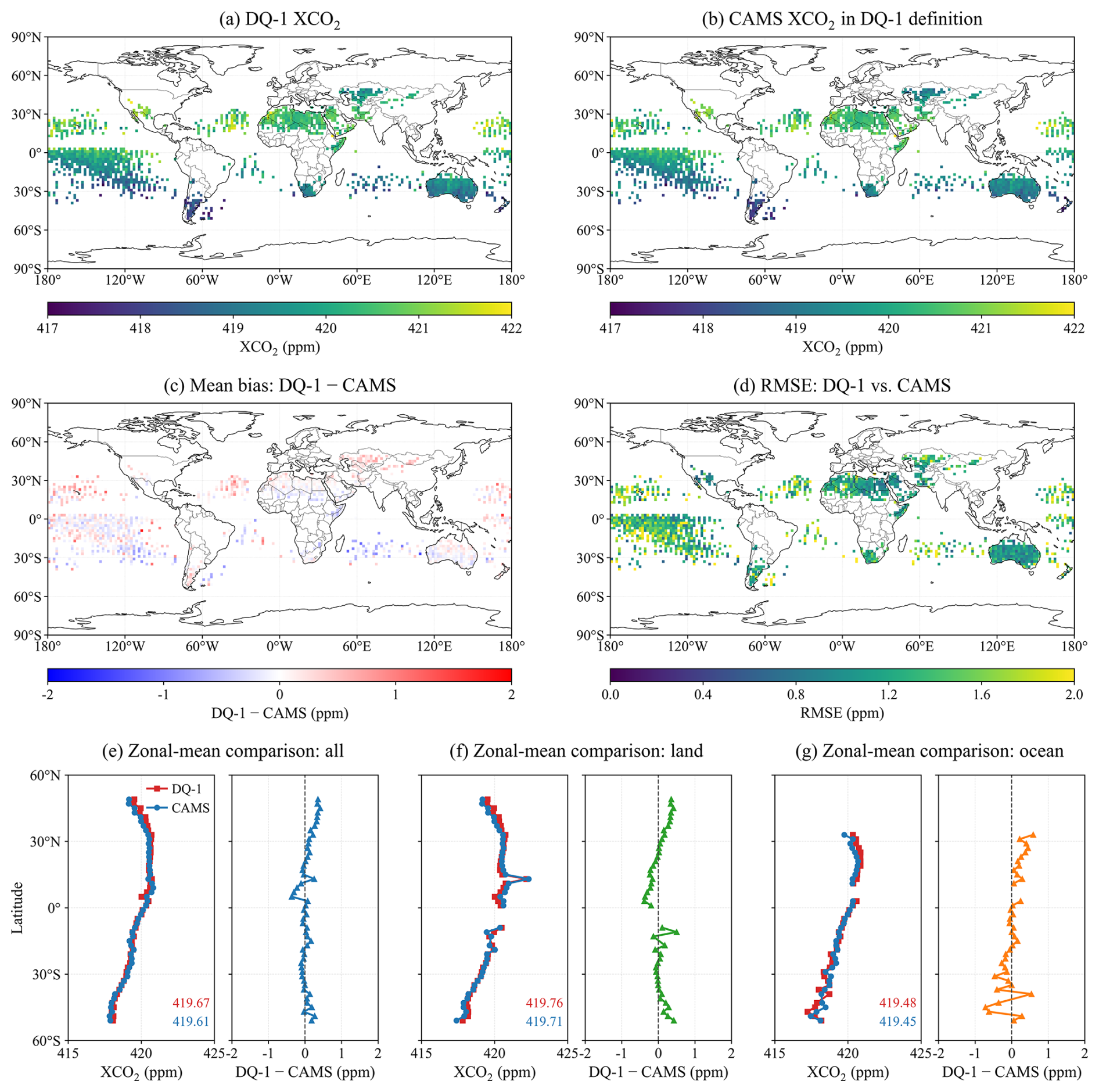
Figure 8 Spatial, residual, and zonal comparisons between nighttime DQ-1 XCO₂ and CAMS-derived XCO₂ under the DQ-1 column definition. (a, b) Spatial distributions of nighttime DQ-1 XCO₂ and CAMS-derived XCO₂, respectively. (c, d) Spatial distributions of the mean bias and RMSE. (e–g) Zonal-mean comparisons for all, land, and ocean samples.

The spatial distribution of RMSE shows generally smaller discrepancies over land, with most land grid cells below approximately 1.2 ppm. Higher RMSE values occur over the tropical Pacific, the Southern Hemisphere oceans, and some coastal regions. Because CAMS-derived XCO₂ is used here as an external model reference rather than observational truth, these spatial differences alone do not identify the source of the residuals.

The zonal-mean comparisons show consistent latitudinal variations between DQ-1 and CAMS. For all samples, the mean XCO₂ values of DQ-1 and CAMS are 419.67 and 419.61 ppm, respectively. The corresponding values are 419.76 and 419.71 ppm over land, and 419.48 and 419.45 ppm over ocean. The mean differences are therefore smaller than 0.1 ppm for all three sample groups. The scatterplots further show a strong linear relationship between nighttime DQ-1 XCO₂ and CAMS-derived XCO₂ for daily 2° paired samples (Fig. S7 in the Supplement). For all samples, R=0.91, mean bias=0.04 ppm, and RMSE=1.33 ppm. The land samples show better agreement, with R=0.93 and RMSE=1.18 ppm, whereas the ocean samples show larger scatter, with R=0.87 and RMSE=1.50 ppm. Overall, nighttime DQ-1 XCO₂ is broadly consistent with CAMS-derived XCO₂ in terms of spatial distribution, zonal variation, and daily 2° paired statistics, indicating good consistency with the CAMS-derived XCO₂ reference field.

To examine whether a residual daytime retrieval effect is evident at the zonal scale, we compared the ascending-minus-descending (daytime-minus-nighttime) XCO₂ differences in DQ-1 with the corresponding CAMS-derived differences for June and December 2022 (Fig. S8 in the Supplement). Over 60° S–60° N, the differences between the DQ-1 and CAMS-derived day–night signals are +0.09 ppm in June and −0.05 ppm in December, with RMSE values of 0.17 and 0.18 ppm, respectively. The small magnitudes and opposite signs do not indicate a persistent systematic daytime-low bias at the zonal-mean scale. This diagnostic does not fully isolate residual solar-background effects at the individual-column level, but it provides no evidence of a large systematic day–night offset in these two months.

3.6 Monthly regional XCO₂ comparisons in representative regions

Figure 9 shows the monthly regional mean XCO₂ variations of DQ-1, OCO-2, OCO-3, GOSAT, and empirically corrected GOSAT-2 in ten representative regions from June 2022–December 2024. Overall, the five regions in the left column, namely Western America, North Atlantic, Sahara, Equatorial Pacific, and Australia, show relatively good consistency among the satellite products. The five products broadly capture similar seasonal variability and the overall increase in regional XCO₂. Their regional mean XCO₂ values are approximately 419.9–420.9, 419.3–420.8, 418.5–420.5, 418.4–419.7, and 417.3–419.1 ppm in these five regions, respectively. Over Australia, DQ-1 also tends to show higher regional monthly XCO₂ than OCO-2 and OCO-3, consistent in sign with the positive DQ-1–OCO differences identified from the collocated analysis in Sect. 3.4. This indicates that, in regions with relatively stable background conditions and sufficient multi-satellite sampling, DQ-1 active observations are comparable to passive optical XCO₂ products at the monthly regional scale. After empirical correction, GOSAT-2 no longer shows the systematic positive offset evident in the original product, consistent with the TCCON and pairwise comparisons in Sects. 3.2 and 3.3.

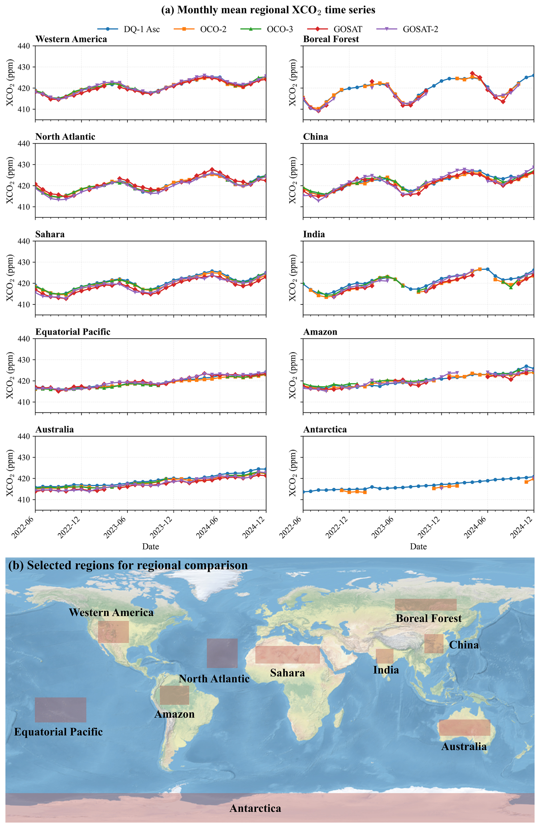
Figure 9 Monthly regional mean XCO₂ time series for selected representative regions and their locations. (a) Monthly mean regional XCO₂ time series from DQ-1, OCO-2, OCO-3, GOSAT, and empirically corrected GOSAT-2. (b) Locations of the ten selected regions used for regional comparison.

The five regions in the right column more clearly highlight the complementary role of DQ-1 relative to passive satellite observations. Passive NIR/SWIR products provide fewer valid monthly XCO₂ values in regions such as the Boreal Forest, India, the Amazon, and Antarctica. These regional sampling differences are interpreted together with the mission-specific sampling characteristics discussed in Appendix A1 rather than being attributed to a single cause. For OCO-3, a separate interruption in data availability was associated with its temporary storage on the International Space Station (ISS), as discussed in Appendix A1 and Fig. A2. Using the criterion that a monthly regional mean is valid only when at least 5 valid observation days are available in that month, DQ-1 provides valid monthly means for all 31 months in all ten regions. In contrast, OCO-3 has no valid monthly means in the Boreal Forest and Antarctica, and only 20 and 22 valid months in India and the Amazon, respectively. The contrast is most evident in Antarctica: DQ-1 provides valid monthly means for all 31 months during the study period, whereas OCO-2 has only 10 valid months, OCO-3 and GOSAT have no valid monthly means, and GOSAT-2 has only 2 valid months.

These results indicate that DQ-1 provides more continuous complementary XCO₂ observational coverage in several high-latitude and passive-observation-limited regions. This finding is consistent with Han et al. (2024), who showed that ACDL/DQ-1 can acquire XCO₂ observations under nighttime, high-aerosol, and high-latitude conditions, suggesting that active IPDA observations can provide an effective complement when passive NIR/SWIR observations are limited.

4 Discussion

4.1 Performance and complementary role of DQ-1 ACDL in satellite XCO₂ observations

The inter-satellite comparisons, TCCON validation, and nighttime model-reference diagnosis consistently show good agreement of DQ-1 ACDL with the corresponding satellite, ground-based, and model references. DQ-1 shows small mean differences relative to OCO-2 and OCO-3, remains consistent with passive optical satellite products in large-scale spatial distributions, meridional structures, and regional monthly variations, and shows daytime TCCON validation performance comparable to that of GOSAT. These results support the use of DQ-1 ACDL as a quantitatively comparable active component of the existing passive optical XCO₂ observing system.

Regional diagnostics further show that the remaining active–passive differences have region-dependent characteristics. Over Australia, the positive DQ-1–OCO differences are accompanied by opposite-signed departures of DQ-1 and the OCO products from the common CAMS-derived reference, whereas over the tropical Pacific the larger scatter is more evident for DQ-1 relative to the same reference. The ocean-surface diagnostics show pair-dependent reflectance relationships and consistent decreases in the wind-speed-binned residual statistics, while substantial grid-cell variability remains. These results indicate that ocean-surface conditions are associated with the residuals, but neither reflectance nor wind speed alone explains their regional spatial structure. DQ-1 also provides complementary XCO₂ sampling under conditions where passive NIR/SWIR observations are limited, particularly at night and at high latitudes. This complementary sampling can help improve the spatiotemporal continuity of satellite greenhouse-gas observations and provide additional support for future active–passive joint XCO₂ analyses, regional carbon flux inversions, and emission monitoring.

4.2 Limitations of the comparison framework

The results should be interpreted within the limitations of the unified comparison framework. First, CAMS CO₂ fields are used for coherent-region selection, estimation of XCO₂ column-definition differences, and nighttime DQ-1 XCO₂ diagnosis. Therefore, the reported differences should be regarded as consistency between satellite products after model-assisted correction for XCO₂ column-definition differences, rather than as a fully model-independent assessment of absolute errors. In addition, daily 2° aggregation and the 4 h temporal matching criterion reduce footprint-scale noise and sampling imbalance, but may smooth real XCO₂ gradients in strong-emission regions, land–ocean transition zones, complex terrain, and regions affected by rapidly changing transport. Although the common comparison-region selection and same-day, same-grid collocation reduce sampling mismatch, the retained pairs still reflect sensor-specific spatial and temporal sampling characteristics. Periods without observations, such as the OCO-3 data gap, do not enter directly into the pairwise statistics but reduce the number of collocations and may alter their spatiotemporal representativeness. Because the primary assessment focuses on coherent and relatively well-sampled regions, the reported inter-satellite agreement is most directly applicable to these conditions. Nevertheless, the P80/P70 and 1–3 h sensitivity tests show that the main statistics remain stable under reasonable changes in the selection and collocation criteria.

Further uncertainties arise from differences in retrieval algorithms, quality filtering, product versions, and bias-correction status among the satellite products. Because the official GOSAT-2 empirical bias correction was developed using TCCON GGG2020 as the reference, the corrected GOSAT-2–TCCON comparison is not fully independent of TCCON. Finally, because TCCON relies on direct solar spectra and therefore does not provide nighttime XCO₂ observations, the nighttime DQ-1 comparison with CAMS-derived XCO₂ should be interpreted as a comparison relative to an external model reference, rather than as an independent observational validation.

5 Conclusions

In this study, we compared DQ-1 ACDL XCO₂ with passive optical satellite XCO₂ products from OCO-2, OCO-3, GOSAT, and GOSAT-2 from June 2022–December 2024. The comparison was conducted within a unified framework that combines CAMS-based spatiotemporal coherence assessment, multi-satellite sampling availability, daily 2° aggregation, spatiotemporal collocation, and correction for XCO₂ column-definition differences. By reducing the influence of sampling representativeness and observation-operator differences, this framework provides a common basis for interpreting inter-product XCO₂ differences.

The results show that DQ-1 ACDL is broadly consistent with OCO-2 and OCO-3 over coherent and well-sampled comparison regions. The mean DQ-1–OCO-2/OCO-3 differences are generally below 0.5 ppm, and the products show similar large-scale spatial distributions, meridional structures, and regional monthly variations. Independent validation against TCCON shows that daytime DQ-1 XCO₂ has a correlation coefficient of 0.92, a mean bias of 0.21 ppm, and an RMSE of 1.49 ppm, with validation statistics comparable to those of GOSAT. The nighttime comparison further shows that, under the DQ-1 column definition, DQ-1 XCO₂ is broadly consistent with CAMS-derived XCO₂. The uncorrected GOSAT-2 retrievals show a clear positive bias, whereas the official empirical correction substantially reduces this bias in both the TCCON and inter-satellite comparisons, highlighting the importance of accounting for product-specific bias-correction status in multi-satellite XCO₂ applications. Ocean diagnostics show pronounced but pair-dependent reflectance associations and consistent decreases in the wind-speed-binned residual statistics, while neither factor alone explains the regional residual pattern, including the elevated RMSE over the tropical Pacific.

Compared with previous studies that mainly evaluated individual XCO₂ products or intercomparisons among passive satellites, the principal contribution of this study is a unified active–passive comparison framework that jointly accounts for background-field coherence, multi-satellite sampling availability, spatiotemporal collocation, and effective XCO₂ column-definition differences. Within this framework, the small differences between DQ-1 and OCO-2/OCO-3 indicate that DQ-1 ACDL XCO₂ is quantitatively comparable to OCO-2 and OCO-3 over the selected comparison regions. These results apply primarily to the selected coherent and well-sampled regions and should be interpreted as product-level consistency after model-assisted treatment of column-definition differences rather than as a fully model-independent assessment of absolute retrieval errors. The nighttime result likewise represents comparison with an external model reference rather than independent observational validation.

Overall, DQ-1 ACDL provides an important active XCO₂ observational capability for the satellite CO₂ observing system. Its agreement with TCCON and product-level consistency with the passive satellite products support its role as a complementary active component of the multi-satellite XCO₂ observing system. In addition, DQ-1 provides complementary sampling at night, at high latitudes, and in regions where passive NIR/SWIR observations are limited. Future work should extend active–passive XCO₂ comparisons at higher spatiotemporal resolution and use joint assimilation and flux-inversion experiments to quantify the added value of combined XCO₂ constraints for regional carbon fluxes and anthropogenic emissions.

Appendix A: Supporting analyses and information

A1 Multi-satellite XCO₂ sampling coverage and temporal variability

Figure A1 shows the cumulative number of valid observations for each satellite product on the unified 2° grid, revealing substantial differences in spatial sampling capability among the sensors. DQ-1 Asc and Desc both show relatively continuous global coverage, with stable sampling coverage between 60° S and 60° N. The two orbital directions exhibit similar spatial patterns but different local sampling intensities, indicating complementary sampling by the ascending and descending observations. OCO-2 provides relatively broad and regular latitudinal coverage because of its sun-synchronous orbit, although orbital-track structure and the effects of observation-mode and quality screening remain evident. In contrast, the precessing ISS orbit of OCO-3 restricts its coverage to approximately 52° S–52° N and produces a strongly nonuniform latitudinal sampling pattern. Sampling density increases toward the orbital turning latitudes near 50°, consistent with the enhanced OCO-3 sampling over parts of North America and Asia in the 40–50° N latitude band seen in Fig. A1 (Taylor et al., 2023). GOSAT and GOSAT-2 exhibit much sparser point-sampling patterns, with GOSAT-2 providing more valid gridded observations than GOSAT, although both remain substantially sparser than the OCO series.

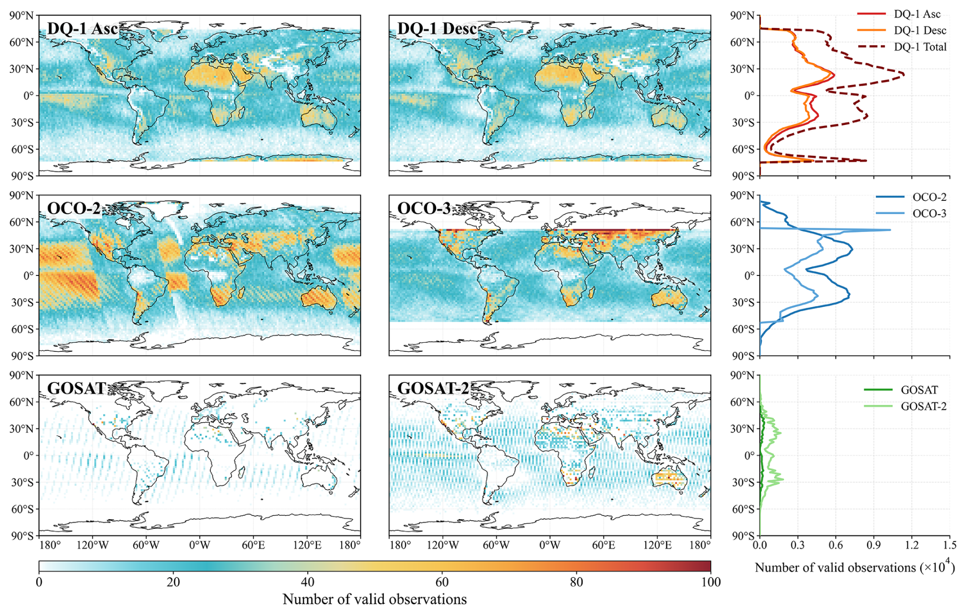
Figure A1 Spatial distributions and zonal totals of cumulative number of valid observations for the satellite XCO₂ products at 2°×2° resolution.

The zonal totals further show that DQ-1 provides more spatially uniform sampling across most latitude bands. The number of valid observations for DQ-1 Total is markedly higher than that for either Asc or Desc alone and exceeds that of any single passive satellite product in most latitude bands. Compared with OCO-2, OCO-3 provides fewer valid observations over much of the ocean, including the tropical Pacific. This pattern is consistent with the lower sampling rate of OCO-3 in glint mode, which is constrained by the pointing geometry and operational requirements of the ISS platform (Taylor et al., 2023). During normal science operations, clouds, aerosols, solar-illumination conditions, and quality screening can further modulate the number of valid passive retrievals, but these retrieval-related effects are distinct from the sampling patterns imposed by orbital and viewing geometry.

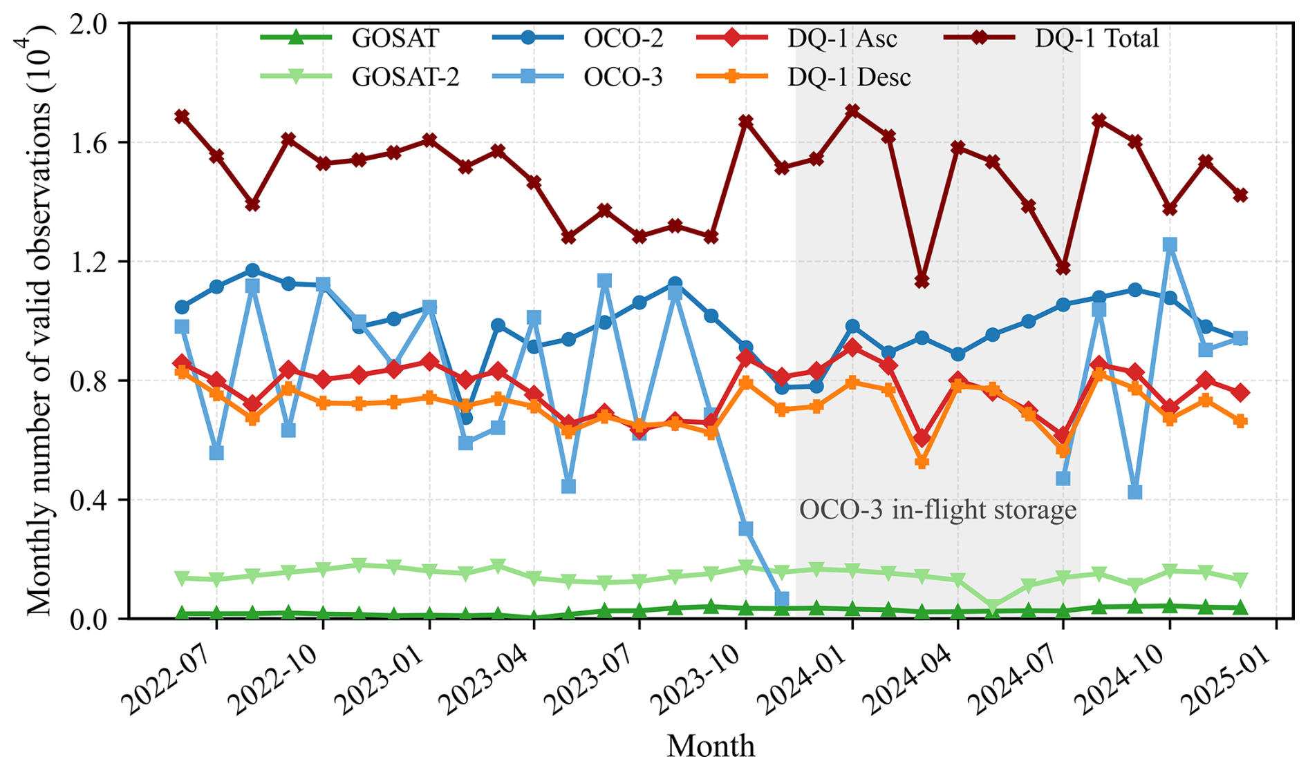
Figure A2 Monthly variations in the number of valid observations for the satellite XCO₂ products. The gray-shaded region indicates the OCO-3 data gap associated with its temporary storage on the ISS.

The monthly statistics are shown in Fig. A2. The mean monthly numbers of valid observations for DQ-1 Asc and Desc are 0.77×10⁴ and 0.71×10⁴, respectively, and the corresponding value for DQ-1 Total is approximately 1.48×10⁴. This value is higher than the corresponding OCO-2 value of 0.99×10⁴. OCO-3 has a mean monthly number of valid observations of approximately 0.61×10⁴ but exhibits substantial month-to-month variability. Reduced sampling is evident in October and early November 2023, followed by a prolonged data gap until mid-July 2024. The gray-shaded region in Fig. A2 marks the OCO-3 data gap associated with its temporary storage on the ISS. This was a mission-level interruption rather than an ocean-specific instrument malfunction. During normal science operations, OCO-3 ocean sampling is additionally constrained by viewing and glint-pointing geometry and ISS operational requirements, while clouds, aerosols, solar-illumination conditions, and quality screening further affect retrieval availability (Taylor et al., 2023). The prolonged data gap nevertheless contributed to the lower overall number of valid OCO-3 observations relative to OCO-2 over the study period.

To assess whether the reduced tropical-Pacific sampling was primarily caused by this interruption, we repeated the comparison using only common-operation full months, excluding October 2023–July 2024. During the remaining 21 months, OCO-2 and OCO-3 provided 17 127 and 8734 valid observations, respectively, corresponding to monthly means of 815.6 and 415.9. OCO-3 sampling therefore remained approximately 51 % of OCO-2 sampling outside the interruption period, indicating that the interruption contributed to, but did not fully explain, the lower tropical-Pacific sampling. We further assessed whether the OCO-3 interruption affected the regional DQ-1–OCO comparison over the tropical Pacific by recalculating the bias and RMSE for the same 21 common-operation months. For DQ-1–OCO-2, the bias and RMSE changed from 0.58 and 1.27 ppm for the full period to 0.61 and 1.26 ppm, respectively; for DQ-1–OCO-3, the corresponding values changed from 0.30 and 1.26 ppm to 0.30 and 1.28 ppm. These small changes indicate that the OCO-3 interruption had little influence on the tropical-Pacific bias and RMSE. GOSAT-2 and GOSAT have much lower mean monthly numbers of valid observations, approximately 0.14×10⁴ and 0.03×10⁴, respectively. Overall, these results highlight the complementarity of multi-satellite observations in spatial coverage and temporal continuity.

A2 Sensitivity of inter-satellite XCO₂ comparisons to spatial-selection and temporal-collocation criteria

Table A1 Sensitivity cases for the spatial-selection and temporal-collocation criteria used in the satellite XCO₂ intercomparison.

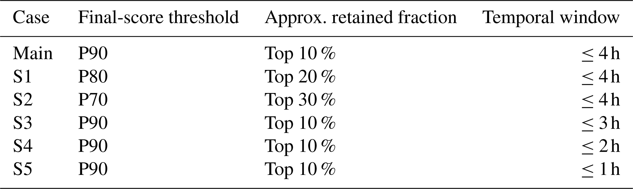
Note: P90, P80, and P70 denote the 90th, 80th, and 70th percentiles of the final score, respectively, calculated separately for land and ocean grid cells. S1–S2 test the spatial-selection criterion, whereas S3–S5 test the temporal-collocation criterion.

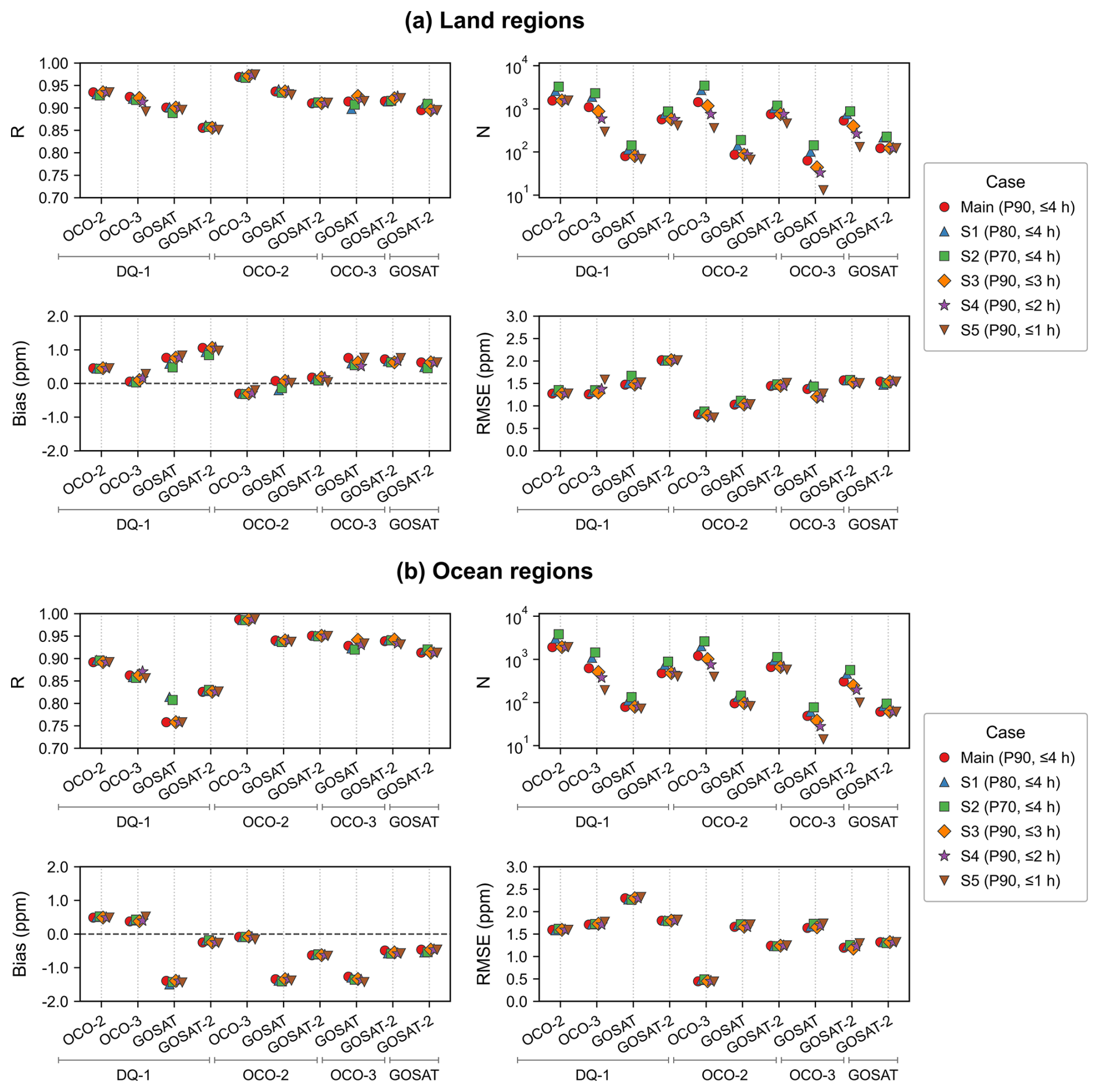
Figure A3 Sensitivity of satellite XCO₂ intercomparison statistics to the spatial-selection and temporal-collocation criteria over (a) land and (b) ocean regions. The four panels for each surface type show the correlation coefficient (R), number of collocations (N), mean bias, and RMSE for the six sensitivity cases defined in Table A1. Satellite pairs are organized by the horizontal brackets: the satellite name below each bracket denotes the first product in the pair, while the individual satellite labels above the bracket denote the second product. Bias is defined as XCO₂(first product)–XCO₂ (second product). Main denotes the reference configuration (P90, ≤4 h); S1–S2 relax the spatial-selection threshold, whereas S3–S5 progressively tighten the temporal-collocation window.

A3 TCCON site information and valid observation periods

Table A2 Abbreviated names, geographic information, and valid observation periods of the TCCON sites used for validation. The valid observation period denotes the overlap between data availability at each site and the study period (1 June 2022–31 December 2024).

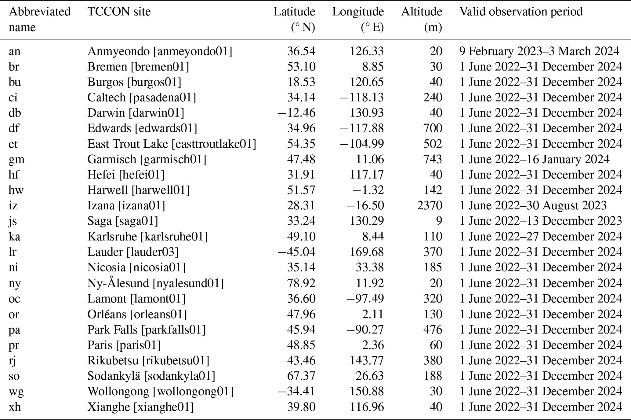
Data references: an: Bu et al. (2026); br: Notholt et al. (2026); bu: Morino et al. (2022b); ci: Wennberg et al. (2022a); db: Deutscher et al. (2023b); df: Iraci et al. (2022); et: Wunch et al. (2022a); gm: Sussmann et al. (2025); hf: Liu et al. (2023); hw: Weidmann et al. (2023); iz: García et al. (2022); js: Shiomi et al. (2022); ka: Hase et al. (2024); lr: Pollard et al. (2022); ni: Petri et al. (2024); ny: Buschmann et al. (2022); oc: Wennberg et al. (2025); or: Warneke et al. (2024); pa: Wennberg et al. (2022b); pr: Té et al. (2022); rj: Morino et al. (2022a); so: Kivi et al. (2026); wg: Deutscher et al. (2023a); and xh: Zhou et al. (2022).