Interacting effects of droplet number and ice formation processes on mixed-phase cold-air outbreak clouds

Shallow, mixed-phase clouds associated with cold-air outbreak (CAO) events are natural laboratories for studying mixed-phase cloud processes which are important for estimating cloud-phase feedback in the warming climate. Recent studies show that CAO clouds are sensitive to aerosol-cloud interactions and ice formation processes, but many modelling studies perturbed model parameters individually, limiting the investigation of joint effects from multiple processes on cloud properties. Here we investigated how six cloud microphysics parameters jointly affect CAO cloud properties by building model emulators trained on output from perturbed parameter ensembles of a high-resolution regional model. The parameters are cloud droplet number concentration (N_d), ice-nucleating particle concentration (N_INP), efficiencies of three secondary ice production processes, as well as the mixed-phase overlap factor (mpof). For the CAO case studied, N_d and N_INP most strongly control the cloud radiative properties in the stratocumulus region; whereas in the cumulus region, effects from varying N_d and mpof are the strongest. Our results show that these parameters have non-linear joint effects such that the magnitude and even sign of cloud responses to a parameter are highly dependent on the values of other parameters. For example, the sensitivity of cloud albedo to increases in N_INP varies between near zero to strongly negative across the sampled parameter space. Therefore, perturbing parameters individually is an inadequate method for determining the cloud responses to model parameters. This work demonstrates the power of model emulation and the importance of a full exploration of parameter space in order to understand the factors controlling cloud properties.

1 Introduction

Low-level, mixed-phase clouds at mid and high latitudes play a key role in the low-cloud optical depth feedback through their phase changes in a warming climate and affect the Earth's radiation budget (Ceppi et al., 2017), which is referred to as the cloud-phase feedback (Mitchell et al., 1989; Storelvmo et al., 2015; Ceppi et al., 2017; Murray et al., 2021). In these mixed-phase clouds, liquid and ice hydrometeors exist at the same time, and the radiative properties of these clouds are strongly controlled by the characteristics and interactions of these hydrometeors at the microphysical scale (Wegener, 1911; Bergeron, 1935; Findeisen et al., 2015; Findeisen and Findeisen, 1943; Pruppacher and Klett, 1996; Korolev et al., 2017). However, because current global climate models are generally poor in representing mixed-phase cloud microphysics (Bodas-Salcedo et al., 2019; Sherwood et al., 2020), uncertainties persist in both the direction and magnitude of the cloud-phase feedback (Sherwood et al., 2020; Zelinka et al., 2020; Forster et al., 2021; Murray et al., 2021). In fact, cloud microphysical processes are subject to large uncertainties due to their highly parametrized and complicated nature (Morrison et al., 2020), even within high-resolution models such as cloud-resolving models and large-eddy simulations.

In this study, we focused on a specific synoptic-scale meteorological event called a cold-air outbreak (CAO). During a CAO event, air masses flow from cold and dry high-latitude continents or ice-covered regions to the warm, open and sea-ice free ocean, leading to instability of the marine boundary layer and strong atmospheric convection for cloud formation (Brümmer, 1996, 1999; Renfrew and Moore, 1999; Kolstad and Bracegirdle, 2008; Kolstad et al., 2009; Fletcher et al., 2016a, b). As the temperature during CAO events is low and normally below 0 °C, extensive mixed-phase clouds form. These mixed-phase CAO clouds have a well-defined flow, which makes them ideal natural laboratories for understanding the mixed-phase processes that are important for modelling the behaviour of mixed-phase clouds under the warming climate. The CAO clouds usually begin with a form of “cloud street” or stratocumulus-like clouds, and then transition into cumulus-like clouds downwind (Brümmer, 1999; McCoy et al., 2017), which can have very different radiative properties (McCoy et al., 2017).

Cloud microphysics strongly controls mixed phase CAO cloud properties. Several high-resolution modelling studies have been conducted to understand the effect of various cloud microphysics processes and parameters on CAO clouds (Field et al., 2014; Abel et al., 2017; Vergara-Temprado et al., 2018; de Roode et al., 2019; Tornow et al., 2021; Karalis et al., 2022; Li et al., 2023; Possner et al., 2024; Huang et al., 2025). These studies show that the cloud properties are very sensitive to aerosols including those that can act as cloud condensation nuclei (CCN) and ice-nucleating particles (INPs), as well as ice formation processes including primary ice production and secondary ice production (SIP). However, all of these studies were conducted by perturbing parameters individually, often called a one-at-a-time (OAT) sensitivity approach. Such an OAT test only allows the responses of cloud properties around a control simulation to be quantified, lacking full exploration of the parameter space and interactions between the parameters. For example, Johnson et al. (2015) has shown that the responses of modelled precipitation in deep convective clouds to the concentration of Aitken and accumulation modes of aerosols and the collection efficiency of drops by graupel are strongly dependent on the values of each other.

A large number of simulations are needed to explore multiple combinations of parameters, which is computationally expensive and impractical for a large number of parameters. To obtain the responses of model variables over the whole parameter space, we applied the approach of model emulation with Gaussian Process (GP) emulators, which is a Bayesian machine learning approach that statistically learns the relationship between model inputs and outputs and acts as a surrogate model of the complex numerical model (Oakley and O'Hagan, 2002; O'Hagan, 2006). The training data are produced by running PPE (perturbed parameter ensemble) simulations of a numerical model, where parameters are perturbed in combinations that are well-designed for training the emulators. The model emulation approach has been recently applied in many complex climate and atmospheric models, including understanding the magnitude and causes of uncertainty in aerosol radiative forcing (Lee et al., 2011, 2012, 2013, 2016; Regayre et al., 2014, 2015, 2018; Johnson et al., 2018; Marshall et al., 2019), assessing potential model simplification of cloud microphysics in global climate models (Proske et al., 2022, 2023), constraining model parametric uncertainties with observations (Johnson et al., 2020; Regayre et al., 2023), identifying the potential existence of structural deficiencies (Regayre et al., 2023; Prévost et al., 2026) and parameter calibration (Elsaesser et al., 2025) in climate models. Besides global models, this approach has also been used in regional models such as investigating the environmental controls on sea breeze circulations (Igel et al., 2018; Park et al., 2020), understanding the controls of cloud properties for deep convective clouds (Johnson et al., 2015; Wellmann et al., 2018, 2020; Hawker et al., 2021) and stratocumulus clouds (Glassmeier et al., 2019; Sansom, 2021; Sansom et al., 2024, 2026). With the model response surface generated from the GP emulators, a variance-based sensitivity analysis (Saltelli et al., 2000) can be applied to quantify the sensitivities of model variables to the investigated parameters.

Here we focus on the influences of aerosol-cloud interactions and ice formation processes on a CAO cloud system over the Labrador Sea on 24 October 2022. This is the warmer case studied in our previous OAT test work (Huang et al., 2025), which showed similar cloud responses to previous studies of aerosol-cloud interactions and ice formation processes in CAO clouds. We explore the joint effects of 6 parameters: (1) fixed in-cloud droplet number concentration, (2) INP concentration, (3–5) three parameters from SIP processes including the Hallett–Mossop process, ice-ice collision and droplet shattering, as well as (6) a parameter controlling the extent of spatial overlap between liquid and ice clouds. The parameters for ice-ice collision, droplet shattering and the extent of spatial overlap between liquid and ice clouds are additional to the parameters studied in Huang et al. (2025). All three SIP mechanisms have been shown to be important for CAO cloud morphology (Karalis et al., 2022) and ice crystal number concentrations in Arctic stratocumulus clouds (Sotiropoulou et al., 2020). It is also suggested that changing the degree of spatial overlap between liquid and ice, which can be estimated with observations, can exert a strong influence on the liquid water path (LWP) and radiative properties of mixed-phase CAO clouds (Abel et al., 2017; Evans et al., 2025).

This paper is structured as follows. In Sect. 2, we describe the numerical model setup, PPE design, training, validation and testing of the GP emulators. In Sect. 3, we present the results starting with example PPE output, and then emulated model responses from the emulators, as well as the multiple OAT tests across the whole parameter space from emulators, followed by summary and discussion on the results of our study compared to previous work, limitations of this study and potential future work in Sect. 4.

2 Methods

Our overall approach was to use PPEs (perturbed parameter ensembles) and GP (Gaussian Process) emulators to understand the joint effects of six cloud microphysics parameters at different stages of a CAO (cold-air outbreak) event. A flow chart of methods involved in this work is shown in Appendix D.

2.1 Model setup and case description

The nested UM (Unified Model) (Brown et al., 2012a) from the UK Met Office was coupled with a double-moment cloud microphysics scheme CASIM (Cloud AeroSol Interacting Microphysics) (Field et al., 2023). We used UM version 13.0 with the RAL (Regional Atmosphere and Land) 3.2 configuration (Bush et al., 2025). The boundary conditions of the nested domains were provided hourly by a global model (N216) with the GAL (Global Atmosphere and Land) 6.1 configuration (Walters et al., 2017). The cloud parameterisation in the nested model was from the bimodal cloud scheme (Van Weverberg et al., 2021a, b). This approach uses subgrid turbulent kinetic energy to diagnose the subgrid humidity distribution and hence cloudy fraction. The cloud cover was derived using cloud fractions in a column with the maximum-random overlap assumption. The radiative processes were from SOCRATES (Suite Of Community Radiative Transfer codes based on Edwards and Slingo) (Manners et al., 2023), and mass mixing ratio and number concentration of ice hydrometeors were both considered when calculating the single-scattering albedo of ice in SOCRATES (Baran et al., 2025). The parameterisation of boundary layer processes in our model is from Lock et al. (2000).

The selected CAO event occurred on 24 October 2022 over the Labrador Sea, which coincided with two flights (C322 and C323) during the M-Phase aircraft campaign (Murray and the M-Phase Team, 2024; Clarke et al., 2026). Figure 1 shows the tracks of both flights, the corresponding nested model domains, and the analysis domains. Flight C322 measured regions dominated by stratocumulus (Sc) clouds, while Flight C323 focused on regions dominated by cumulus (Cu) clouds.

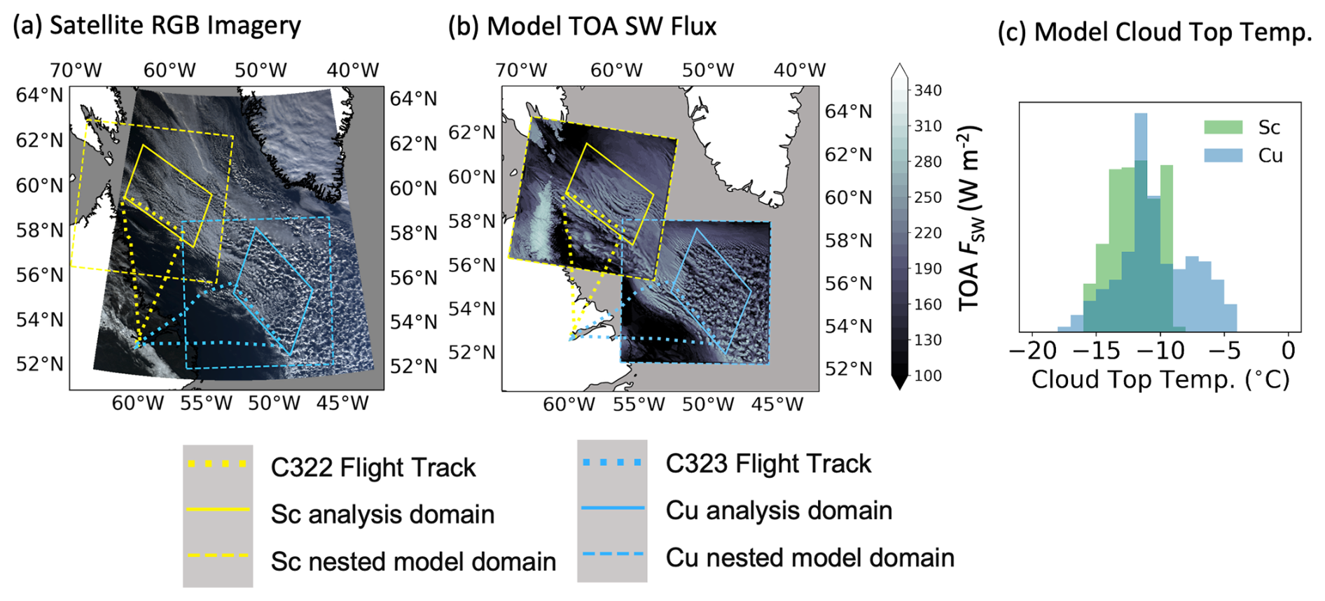
Figure 1 Flight tracks (dotted line), nested model domains (dashed squares) and model analysis domains (solid rectangles) for Sc region (yellow) and Cu region (blue) on 24 October 2022 over the Labrador Sea: (a) the RGB satellite imagery created using bands 1 (620–670 nm), 3 (459–479 nm), and 4 (545–565 nm) from MODIS (Moderate Resolution Imaging Spectroradiometer) Level 1B Calibrated Radiances Product (Collection 6.1) (MODIS Characterization Support Team (MCST), 2017) onboard the Aqua satellite, (b) the SW (shortwave) reflectance at the top-of-the-atmosphere from the control simulations. The selected model time is the same as the satellite retrieval time at 17:00 UTC and the model output fields are instantaneous. Cloud top temperatures in the two analysis domains are shown in (c). The cloud top temperatures were derived using the air temperature at the highest model grid in a column, with a cloudy grid defined using total cloud water content $\ge {\mathrm{10}}^{-\mathrm{6}}$ kg kg⁻¹. The model output time for CTT in the Sc region is 14:00 UTC and is 19:00 UTC in the Cu region for the corresponding times of flights. The temperature profiles were evaluated in our previous work (Huang et al., 2025).

Both nested model domains contain 500×500 gridpoints with a horizontal grid spacing of 1.5 km, centred at 60° N, 60.5° W for capturing the early stage and Sc region and 56° N, 51° W for the Cu region. Field et al. (2017) has demonstrated that this grid spacing is capable of reproducing the general cloud features of a CAO event. The nested model domains were designed to ensure the model analysis domains remained sufficiently distant from the domain boundaries, allowing cloud fields to fully develop when they leave the ice edge and before entering the model analysis domains. At this point, the model has already spun up from the boundaries. The regional model has 90 vertical levels capped at 40 km with 16 model levels below 1 km and 28 model levels below 3 km. The model is set to the atmosphere-only configuration with prescribed sea surface temperature (SST) and fixed surface fluxes. The mean SST in the Sc region is 277.5 K and is 280.5 K in the Cu region.

The simulations were initialized at 00:00 UTC and performed for 24 h, with the model output from the first 12 h excluded from the analysis due to model spin-up.

2.2 Perturbed parameters and PPE design

Six parameters were investigated in this study: N_d (cloud droplet number concentration), $N_{\text{INP}}^{-\mathrm{15}}$ (INP concentration at −15 °C), E_HM (efficiency of the Hallett–Mossop process), E_BR (leading coefficient controlling the efficiency of the ice-ice collisional breakup process), E_DS (efficiency of the droplet shattering process), and mpof (mixed-phase overlap factor). All the parameters are within the CASIM scheme. A description of each perturbed parameter and the selection of their perturbed ranges are introduced in this section. The combinations of the six parameter values were designed with the maximin Latin hypercube sampling method. The single OAT test was performed for every parameter before running the PPEs to investigate the effects of perturbing each parameter individually around the control simulation (not shown).

Figure 2 shows the five hydrometeors and the main processes in CASIM with relevant processes for the perturbed parameters in this work highlighted. Not all processes in CASIM are shown here (e.g. self-collection, sedimentation, evaporation and sublimation); see Field et al. (2023) for a complete description of CASIM implementation in the UM. To keep the consistency of symbols, we used the same symbol for mass tendency (P) and number tendency (N) in the description of parameters below. In CASIM, cloud ice is represented as a spherical particle (m∝D³, where m is mass and D is diameter of a hydrometeor) and snow is represented as aggregate particles (m∝D²) based on findings from Cotton et al. (2013) (Field et al., 2023). Details for terminal fall speed, mass-dimension and shape of the particle size distribution of each hydrometeor in CASIM can be found in Table A1 in Field et al. (2023) and the calculation of the ventilation coefficient is presented in Eq. (A23) in Field et al. (2023).

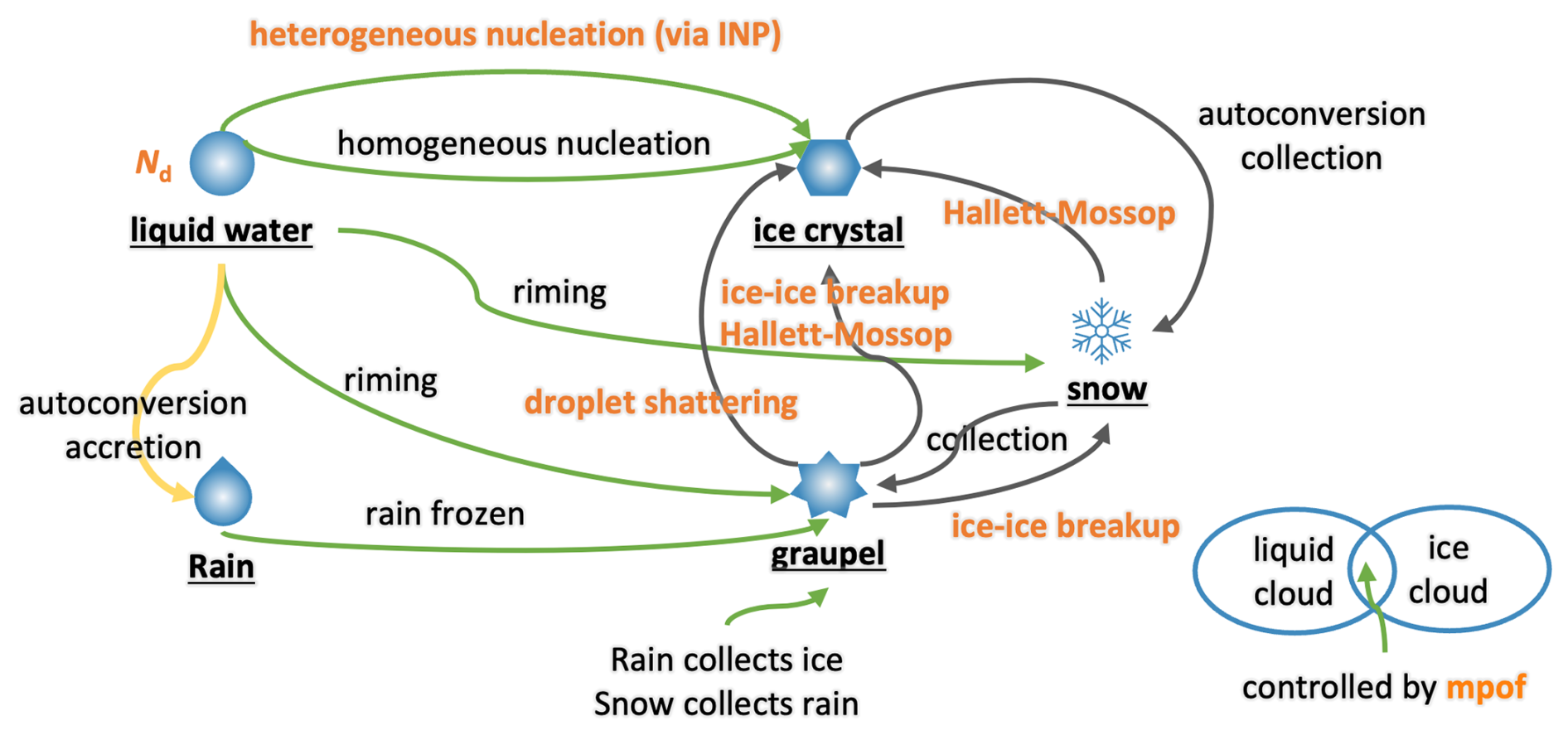
Figure 2 Key processes among the five CASIM hydrometeors: liquid water, rain, ice crystal, snow and graupel. Processes which contain the parameters investigated in this work are highlighted in orange. Liquid-liquid processes are highlighted in yellow, mixed-phase processes are highlighted in green and ice-ice processes are in dark grey. Details of the treatment of SIP processes are shown in the Methods section. Not all the cloud microphysical processes in CASIM are shown here; see Field et al. (2023) for detailed information about the implementation of CASIM in the UM.

2.2.1 N_d (cloud droplet number concentration)

N_d is a fixed vertical profile of in-cloud droplet number concentration set in CASIM if aerosols are not used for deriving the cloud droplet number concentration. We did not select the option to use aerosol-derived N_d in this study to avoid extra complexity for parameter perturbation and model output interpretation. N_d was set to 35 cm⁻³ in the control simulation and perturbed over the range from 5 to 75 cm⁻³ in the PPE design to cover the observed N_d ranges calculated using satellite retrievals from MODIS instrument onboard the Aqua satellite with the method from Grosvenor et al. (2018) (Fig. 3a). The satellite-derived N_d ranges agree well with the N_d ranges from the CDP (cloud droplet probe) instrument onboard M-Phase C322 and C323 (Fig. 3a). The 1 Hz CDP measurements were averaged to match the model resolution (1.5 km) and those with N_d less than 1 cm⁻³ were removed before averaging.

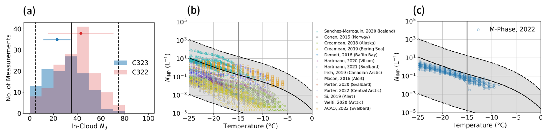
Figure 3 Comparison between the perturbed range and the measurements: (a) N_d with measured in-cloud N_d from M-Phase C322 and C323 using the CDP (cloud droplet probe) onboard, and N_d (mean ± one standard deviation) calculated based on retrievals from MODIS instrument onboard the Aqua satellite; (b) perturbed temperature-dependent N_INP ranges compared to INP measurements at high latitudes in the Northern Hemisphere (Sanchez-Marroquin et al., 2020; Franz Conen, 2016; Creamean et al., 2018, 2019; DeMott et al., 2016; Hartmann et al., 2020, 2021; Irish et al., 2019; Mason et al., 2016; Porter et al., 2020, 2022; Si et al., 2019; Welti et al., 2020; Raif et al., 2024); (c) perturbed temperature-dependent N_INP ranges compared to all INP measurements from the M-Phase campaign (Tarn et al., 2025). Boundaries of each perturbed range (maximum and minimum values) are shown with dashed black lines, and the values used for the control simulations are shown with solid black lines. Cloud top temperatures are around −15 °C for the CAO clouds in this case and −15 °C is marked with bold gray solid line in (b) and (c).

The range of N_d was chosen to understand how much the variation of N_d in a CAO event affects the cloud properties, which arises from the natural variability of aerosols and limited by the fixed N_d setup. We did not select the bigger range as in Huang et al. (2025) because the domain-mean N_d can be constrained approximately from satellite retrievals (e.g. Grosvenor et al., 2018).

2.2.2 $N_{\text{INP}}^{-\mathrm{15}}$ (INP concentration at −15 °C)

INP concentration (N_INP) was perturbed by scaling a temperature-dependent INP parameterisation as shown in Fig. 3b and c. The temperature-dependent INP parameterisation over the Labrador Sea region was derived based on n_s(T) (active site density) parameterisations for sea-spray aerosols (McCluskey et al., 2018) and soil dusts (see Appendix A) that accounts for the biogenic component associated with the dust (Herbert et al., 2025). The sea-spray aerosol and dust concentrations from a separate global model over the Labrador Sea region during the M-Phase aircraft campaign period were used with the above parameterisations to derive the temperature-dependent INP parameterisation in this study. The global model used for the aerosol concentrations was performed with a global configuration of the UM (Brown et al., 2012a) version 12.1 which includes Global Atmosphere version 8.0 and Global Land model version 9.0 (Willett et al., 2026). Appendix B shows the details of the global model and the INP concentration in the control simulation, which agrees well with INP measurements from the M-Phase aircraft campaign as in Fig. 3c.

N_INP in the regional model was directly linked to the number concentration of ice crystals produced by heterogenous ice nucleation, assuming that one INP produces one ice crystal. No aerosols were included for the INP calculation in the regional model. Therefore, when perturbing N_d and N_INP, we are effectively directly changing cloud hydrometeor concentrations rather than explicitly modelling the interaction between evolving aerosol fields and clouds. We chose to not use aerosol-interactive N_d and N_INP in this study to reduce the complexity of interpretation over the multi-dimensional parameter space and the computational resources required for running a large number of simulations for PPEs. However, there are several limitations of such choice (e.g. missing potential feedback with aerosol processing) which are further discussed in the Discussion and Conclusions.

INP concentrations were perturbed by the same scale factor at all temperatures. For ease of reference to typical values we define the parameter in the PPE as $N_{\text{INP}}^{-\mathrm{15}}$ (INP concentration at −15 °C, L⁻¹), which is around 0.17 L⁻¹ (170 m⁻³) in the control simulation. The range of $N_{\text{INP}}^{-\mathrm{15}}$ in the PPE is shown in Fig. 3b. The $N_{\text{INP}}^{-\mathrm{15}}$ were perturbed with a range from $\mathrm{1.7}\times {\mathrm{10}}^{-\mathrm{5}}$ L⁻¹ (0.017 m⁻³) to 17 L⁻¹ (17 000 m⁻³) (factor of 0.0001–100 relative to the control value).

Such a large range of INP concentration (six orders of magnitude) was selected to represent the range of possible INPs based on our knowledge prior to the in-situ measurements of INPs from the aircraft campaign. This is because, unlike N_d, the INP concentration cannot be constrained using satellite retrievals or other remote-sensing observations. The ranges for N_d and N_INP were therefore based on different sources of information available before the aircraft campaign. The aim was to examine how these natural ranges in these two quantities interactively affect CAO clouds.

2.2.3 E_HM (efficiency of the Hallett–Mossop process)

The Hallett–Mossop process (also called rime splintering) produces small ice splinters during the riming of liquid droplets onto existing ice hydrometeors (Hallett and Mossop, 1974). The efficiency of the Hallett–Mossop process (E_HM) is defined as the number of splinters produced per milligram of rimed liquid, with the mass of each splinter (M_I0) set as 10⁻¹⁸ kg. The mass tendency of ice created by the Hallett–Mossop process in CASIM (P_ihal) is based on the mass tendencies of graupel-cloud water (P_gacw) and snow-cloud water riming (P_sacw) with the number of splinters per milligram of rime varying according to a triangular function (f(T)) between −2.5 and −7.5 °C (outside of which the value is zero) with the peak at −5 °C (Field et al., 2023).

$$\begin{array}{}\text{(1)}& {\displaystyle }{\displaystyle }{P}_{\text{ihal}}=E_{\text{HM}}{M}_{\text{I0}}(P_{\text{gacw}}+P_{\text{sacw}})f\left(T\right)\end{array}$$

E_HM was set to 350 mg⁻¹ in the control simulation and perturbed from 35 to 3500 mg⁻¹ (factor of 0.1–10). This range was defined based on previous findings that simulations with a factor of 10 higher efficiency than the default value agree well with observed ice crystal number concentrations (Young et al., 2019). The lower limit was chosen to ensure that the default value remains sufficiently distant from the boundary of the parameter space, where emulator predictions are typically subject to higher uncertainties. The multiple OAT test (Sect. 3.3) and global sensitivity analysis (Appendix G) were performed with a different range of E_HM from the range of PPE design, which is from 350 to 3500 mg⁻¹ rather than from 35 to 3500 mg⁻¹.

2.2.4 E_BR (coefficient controlling the efficiency of the ice-ice collisional breakup)

E_BR is a coefficient controlling the efficiency of the ice-ice collisional breakup (χ_BR), which is the number of fragments produced from hydrometeor collisions. The number tendency of ice-ice collisional breakup (N_iics,xy, where x denotes the colliding hydrometeor and y the hydrometeor being collided with) used in this study follows the temperature-dependent approach in Takahashi et al. (1995) and Sullivan et al. (2018).

$$\begin{array}{}\text{(2)}& {\displaystyle }& {\displaystyle }{N}_{\text{iics},xy}=-{\mathit{\chi }}_{\text{BR}}{N}_{\text{xacy}}\text{(3)}& {\displaystyle }& {\displaystyle }{\mathit{\chi }}_{\text{BR}}=E_{\text{BR}}(T-T_{\text{min}}{)}^{\mathrm{1.2}}\exp \left[-{\displaystyle \frac{(T-T_{\text{min}})}{{\mathit{\gamma }}_{\text{BR}}}}\right]\end{array}$$

The minimum temperature (T_min) for ice-ice break-up is set at −21 °C and a decay rate (γ_BR) of fragment number at warmer subzero temperatures is set to 5. The collisions involve ice and snow particles breaking up through collisions with graupel. N_xacy are the existing number tendencies from graupel collecting ice and graupel collecting snow. Detailed description of mixed-phase and cold-phase collection between particles of different hydrometeors in CASIM can be found in Field et al. (2023).

E_BR was set to 280 in the control simulation and perturbed with a range from 2.8 to 2800 (factor of 0.01–10 relative to the control value). The lower limit of the perturbation range is similar to the scaling factors in Sotiropoulou et al. (2020), considering that the original value from Takahashi et al. (1995) overestimates the number of fragments as their experiments were conducted with hails. Although the upper limit is highly unlikely for ice and snow particles due to the excessive number of fragments it implies, it was retained to ensure that the default value remains sufficiently distant from the boundary of the parameter space, where emulator predictions are generally associated with greater uncertainties. The multiple OAT test (Sect. 3.3) and global sensitivity analysis (Appendix G) were performed with the realistic range of E_BR from 2.8 to 280.

Compared to the parameterisation from Phillips et al. (2017), which is based on collision kinetic energy, our approach here is simplified and only considered the broad type II of collision with graupel. Such choice was made to avoid extra complexity for parameter perturbation of the ice-ice collision process and future work is recommended to investigate with the parametrization from Phillips et al. (2017) for a more comprehensive understanding of the role of ice-ice breakup.

2.2.5 E_DS (efficiency of the droplet shattering process)

During the freezing of large supercooled droplets, the pressure inside the freezing droplets increases which can lead to the breakup of the frozen droplets and ice crystal formation (Leisner et al., 2014). Our approach follows the droplet shattering parameterisation from Sullivan et al. (2018), in which the droplet shattering tendency is dependent on the number of fragments produced for each droplet shattering (E_DS), a temperature-dependent shattering probability (p_DS) and the Bigg droplet freezing rate (Bigg, 1953) (N_Bigg). The equation below shows the calculation of the number tendency of ice (N_idps) from the droplet shattering process. Details on p_DS can be found in Sullivan et al. (2018) and the Bigg droplet freezing in CASIM can be found in Field et al. (2023).

$$\begin{array}{}\text{(4)}& {\displaystyle }{\displaystyle }{N}_{\text{idps}}=(\mathrm{1}+p_{\text{DS}}{E}_{\text{DS}})N_{\text{Bigg}}\end{array}$$

The shattering probability was set to the same as the default one in Sullivan et al. (2018) with the shattering probability centred at −15 °C and the maximum probability set at 20 %. E_BR was set to 5 in the control simulation with a perturbed range from 2 to 10 in the PPE design, following the sensitivity test values in Sullivan et al. (2018).

2.2.6 mpof (mixed-phase overlap factor)

When both ice and liquid clouds exist in the same model grid box, the mpof (mixed-phase overlap factor) is used for determining the extent to which ice and liquid co-exist in the same air in CASIM, which is important for mixed-phase processes (Field et al., 2023; Evans et al., 2025). We followed the naming of this parameter the same as in Field et al. (2023) and Evans et al. (2025) for consistency.

The mpof controls a function that quantifies the fractional overlap during the run time of the model rather than being a fixed value in a model grid box. When mpof is 1, the sub-grid liquid and ice cloud are maximally overlapped. When mpof is 0, the sub-grid liquid and ice are not overlapped as long as ${\text{CF}}_{\text{liq}}+{\text{CF}}_{\text{ice}}<\mathrm{1}$, where CF refers to cloud volume fraction in a model grid box. Once the combined cloud fraction goes above 1, there will be overlap. For an mpof of 0, the overlap is minimised. Values of mpof in between lead to increasing overlap, but once either the liquid or ice cloud fraction reaches 1, then mixed-phase overlap is maximum whatever mpof is set to. See Sect. A.6 in the documentation of CASIM implementation in the UM from Field et al. (2023) for more information. The mpof was set to 0.5 in the control simulation with a perturbed range from 0 to 1 in the PPE design.

2.2.7 Parameter design of PPE members

The maximin Latin hypercube sampling method was used to generate random combinations of parameter values across the 6-dimensional space for PPE simulations. The ranges of each parameter are discussed above. The maximin design maximizes the minimum distances between the points in parameter space. Each PPE contains 66 members following the guidance from Loeppky et al. (2009) that at least 10×n (where n is the number of parameters) simulations are required for training GP emulators. Two 6-member testing sets of simulations were also performed with parameter values from another maximin Latin hypercube sampling design. The testing simulations were used for assessing the performance of emulators trained with PPE output. The values of parameters in the testing simulations were different from the ones in the PPE simulations which were used for training the emulators. Figure 4 shows the PPE and testing set input values.

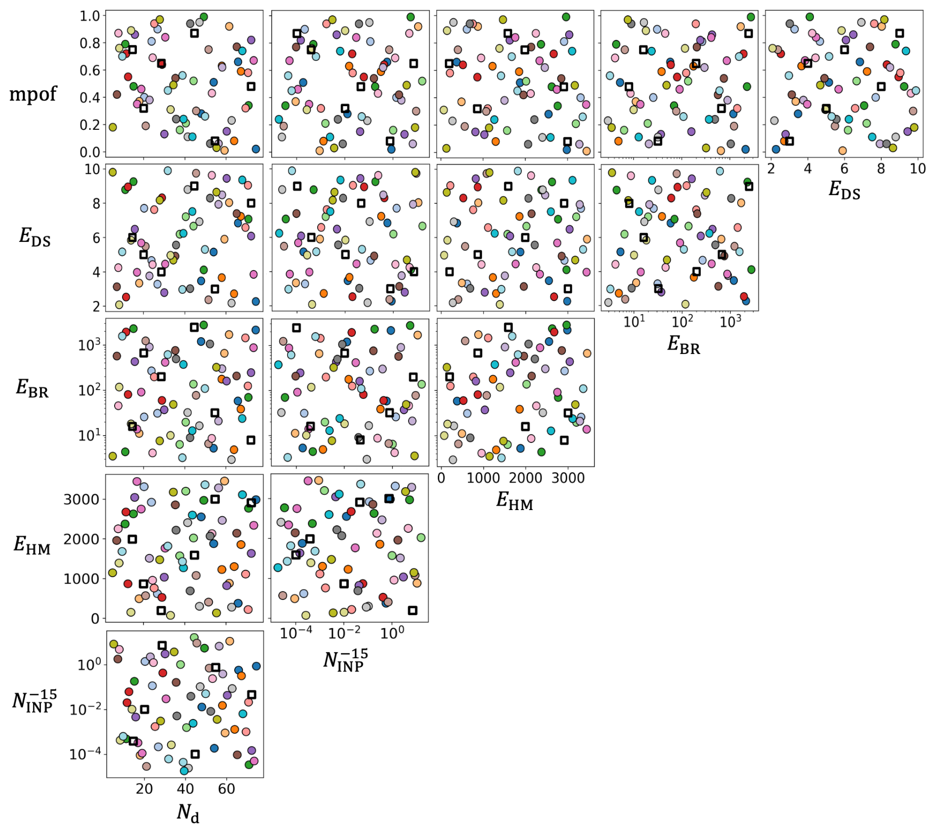
Figure 4 Paired combinations of parameters perturbed in this study. Colour filled circles are the 66 PPE members used for training the GP emulators, and the unfilled squares are the six testing members used for testing the trained GP emulators. Each colour suggests a set of parameter values. Results of kernel selection, validation and testing are shown in Appendix C.

2.3 Gaussian Process (GP) emulators

Gaussian Process (GP) emulation is a non-parametric supervised machine learning method that learns the relationship between model input parameters and outputs of interest (Oakley and O'Hagan, 2002; O'Hagan, 2006). GP emulators were constructed on the output from the PPE simulations and acted as a statistical “surrogate” model for the computationally-expensive numerical model. The GP emulators enabled efficient exploration of the entire parameter space with dense sampling, allowing for construction of multi-dimensional response surfaces and a variance-based sensitivity analysis to assess the importance of the perturbed parameters to the cloud variables. Detailed methodologies and explanations on building GP emulators for climate and atmospheric models can be found in Lee et al. (2011) and Johnson et al. (2015).

A GP emulator consists of a mean function and a covariance function, also called the kernel. To obtain a good GP emulator of each variable of interest we tested four commonly-used stationary kernels: the Radial Basis Function (RBF) kernel and three Matérn kernels with different smoothness parameters: the Matérn12 kernel (0.5), the Matérn32 kernel (1.5), and the Matérn52 kernel (2.5), implemented in the GP Jax Python library for Gaussian processes (Pinder and Dodd, 2022). When the smoothness parameter becomes infinite in a Matérn kernel, it becomes equivalent to the RBF kernel. For each variable, we conducted cross-validation by dividing the 66 PPE members into 11 sets with 60 training and 6 validation data points per set. The cross-validation was used here to maximise the use of our limited data due to the high computational cost of running the numerical simulations. Emulator performance was assessed with graphical diagnostics including individual standardized error plots and Q-Q plots following the guidance from Bastos and O'Hagan (2009), as well as the RMSE (root mean squared error) and R² (coefficient of determination). The kernel selection was mainly based on the RMSE values, with the Q-Q plots and R² for supporting the assessment. Once the best-performing kernel was selected for each variable, we trained the GP emulator with the best kernel on all 66 PPE members and tested it with the corresponding testing set. Appendix C describes and discusses the emulator performances from the kernel selection and testing steps, as well as the dependency of the RMSE on the different numbers of training points.

3 Results

3.1 Example response from PPE simulations: TOA albedo

Before analysing emulated response surfaces of domain-mean outputs in the next section, we first illustrate the strength of perturbing parameters in a PPE design and use TOA albedo here as an example in Fig. 5. Note that the emulators (Sect. 3.2) define the relationship between input parameters and mean output variables (e.g. domain-mean albedo) and cannot describe the specific cloud patterns shown here, hence why we start by showing the results of some PPE members. We selected two parameters to demonstrate the PPE results: N_d and $N_{\text{INP}}^{-\mathrm{15}}$ for the Sc region, and N_d and mpof for the Cu region. These parameter pairs were chosen only for illustration because, as we show in Sect. 3.2, they have the strongest joint effects on cloud albedo in each region.

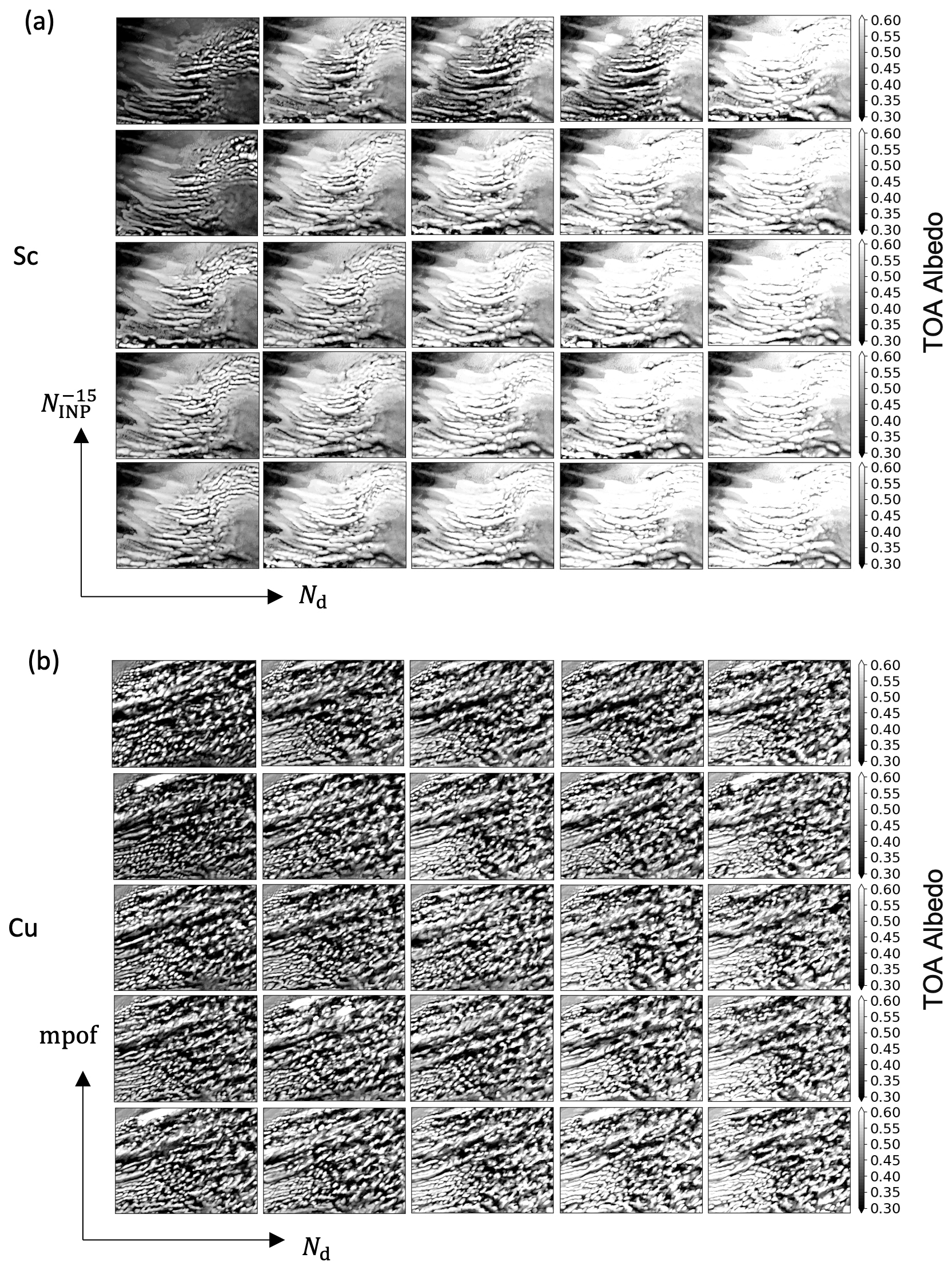
Figure 5 Responses of TOA albedo for maps of (a) the Sc region ordered according to N_d and $N_{\text{INP}}^{-\mathrm{15}}$ and (b) the Cu region ordered according to N_d and mpof. The selected model output time is 16:00 UTC. The selected domains are the same as the regions shown in Fig. 1. Note that each image shows a different simulation, and only 25 out of the 66 PPE parameters are shown here. Because of the Latin hypercube design method used for sampling the parameter space, the subplots shown here are only ordered using the values of the selected two parameters with the values of other four parameters ignored and the intervals between of these subplots for each parameter are not the same.

Figure 5 shows the maps of TOA albedo in 25 of the 66 PPE simulations over the two regions. The intervals between each PPE output are not equal in Fig. 5 because of the Latin hypercube design method used for sampling the parameter space, and the subplots shown in Fig. 5 are only ordered using the values of the selected parameters with the values of other four parameters ignored.

In both regions, the selected parameters jointly affect the TOA albedo. For example, in the Sc region (Fig. 5a), low N_d and high $N_{\text{INP}}^{-\mathrm{15}}$ (top left subplot) result in the lowest TOA albedo, while high N_d and low $N_{\text{INP}}^{-\mathrm{15}}$ (bottom right subplot) result in the highest TOA albedo. With PPE simulations, we can see clear joint effects of parameters on cloud properties. However, the number of simulations is too small to identify whether the joint effects are linear (combined effects) that could be predicted from combinations of OAT simulations, or non-linear (interactive effects) (Sansom, 2023). See Appendix E for a simple illustration of linear and non-linear joint effects between two parameters. Using the emulators enables a much denser sampling of the parameter space and, as we show in Sect. 3.2, exposure of non-linear effects (interactions) of combinations of parameters that are not apparent in Fig. 5.

3.2 Emulated model response surface

The PPE members provide considerable information about cloud behaviour across the 6-D parameter space, but the data sparseness (just 66 points in 6-D space) limits our ability to visualise joint parameter effects or to perform statistical analysis. Therefore, we built emulators of temporally and spatially averaged cloud properties, which enable 6-D continuous response surfaces to be created. The time of averaging for variables (except the cloud top temperature) is from 12:00 to 19:00 UTC, and the domains of averaging are shown as analysis domains in Fig. 1. Cloud top temperature (CTT) is derived from the air temperature at the highest model level in a column with total cloud water content $\ge {\mathrm{10}}^{-\mathrm{6}}$ kg kg⁻¹. The model output is taken at 14:00 UTC for the Sc region and 19:00 UTC for the Cu region, corresponding to the times of the M-Phase C322 and C323 flights respectively. An evaluation of modelled air temperature against aircraft measurements can be found in Huang et al. (2025). The response surfaces were generated by predicting one million output values from the emulators across the parameter space.

Figure 6 shows the distributions of TOA albedo, cloud cover, all-sky LWP (liquid water path), all-sky IWP (ice water path), all-sky TWP (total water path), and CTT from one million combinations of parameters drawn from the GP emulators. By perturbing all 6 parameters in the Sc region, the TOA albedo ranges from 0.43 to 0.54 (inter-percentile range from 5 % to 95 %), cloud cover from 0.84 to 0.91, LWP from 74.5 to 149.5 g m⁻², IWP from 0.0 to 38.1 g m⁻², TWP from 97.6 to 148.4 g m⁻² and CTT from −12.3 to −11.2 °C. In the Cu region, the TOA albedo ranges from 0.37 to 0.44, cloud cover from 0.78 to 0.84, LWP from 47.9 to 98.4 g m⁻², IWP from 71.3 to 186.1 g m⁻², TWP from 147.8 to 244.4 g m⁻² and CTT from −11.0 to −9.3 °C.

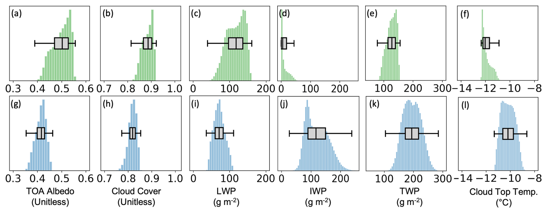
Figure 6 Distributions of cloud variables from 1 million combinations of parameter values for (a, g) all-sky TOA albedo (unitless), (b, h) cloud cover (unitless), (c, i) all-sky LWP (g m⁻²); (d, j) all-sky IWP (g m⁻²), (e, k) TWP (g m⁻²) which is the sum of LWP and IWP, and (f, l) cloud top temperature (°C). Separate distributions are shown for the Sc (top row) and Cu (bottom row) regions.

Figures 7 and 8 show the joint effects of each combination of two parameters with the other parameter effects averaged for TOA albedo and all-sky LWP, which are two key properties for cloud-phase feedback, respectively over the two selected regions. These are known as “paired projections”. Paired projections for cloud cover, all-sky IWP, all-sky TWP, and CTT are shown in Appendix F. The values shown on the paired projection plots are calculated by averaging over the other four dimensions, and therefore describe the mean response of each variable to each paired parameter set.

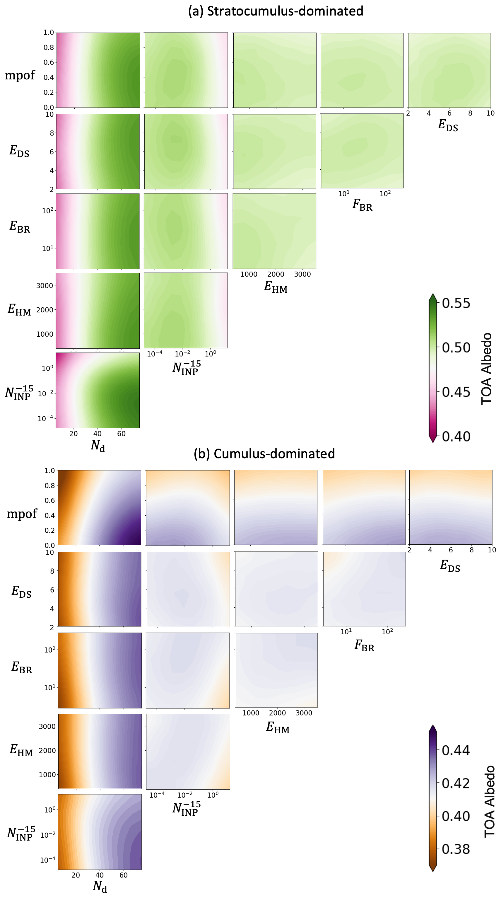
Figure 7 Emulated mean model responses of all-sky TOA albedo to paired parameters in (a) the Sc region and (b) the Cu region. The values shown on the paired projection plots are calculated by averaging over the other four dimensions, and therefore describe the mean response of each variable to each paired parameter set.

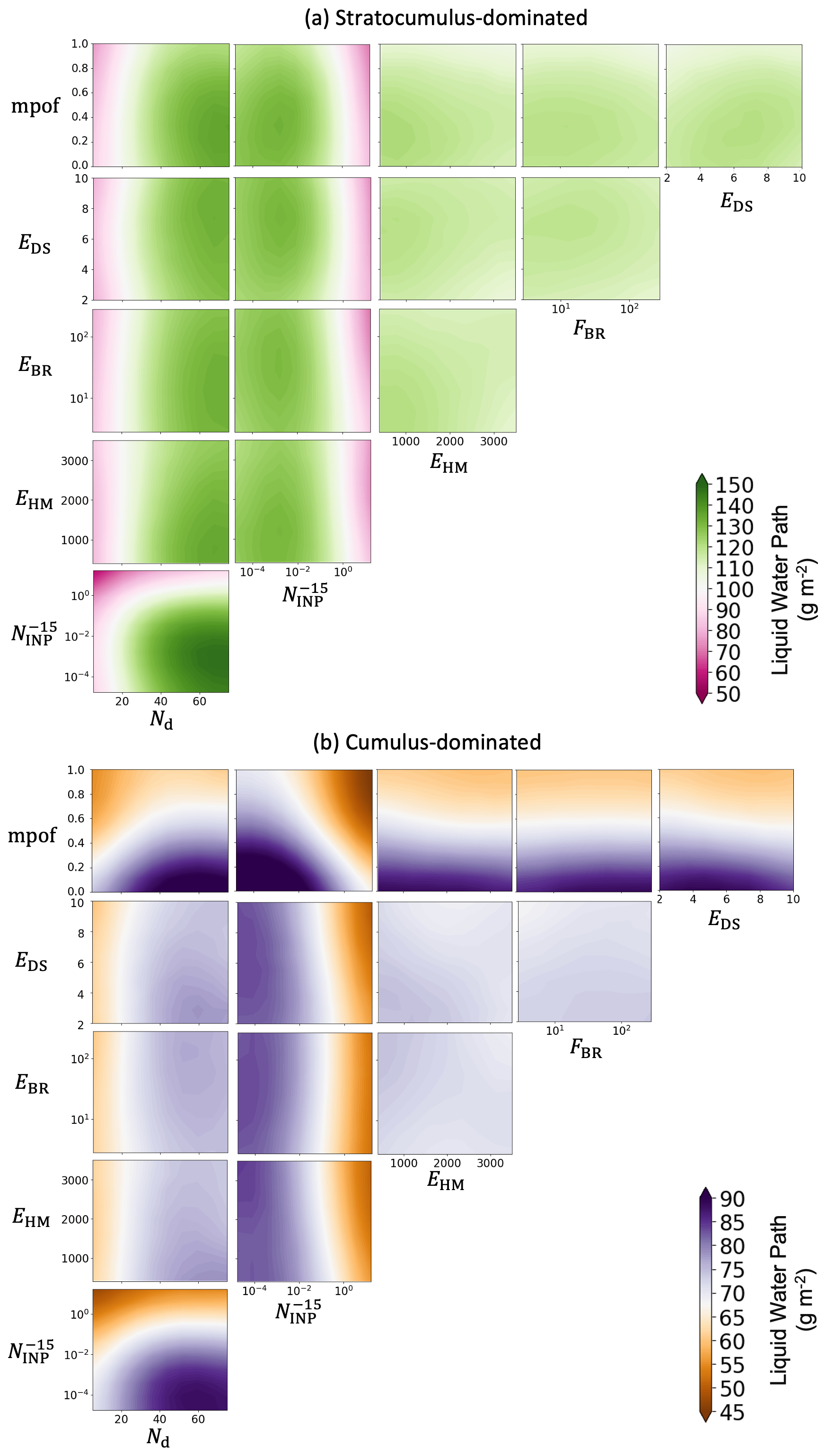
Figure 8 Emulated mean model responses of all-sky LWP to paired parameters in (a) the Sc region and (b) the Cu region. The values shown on the paired projection plots are calculated by averaging over the other four dimensions, and therefore describe the mean response of each variable to each paired parameter set.

Using the paired-projections, we are able to qualitatively identify key parameters controlling the cloud properties over the parameter space in this CAO event. In the Sc region, N_d and $N_{\text{INP}}^{-\mathrm{15}}$ exert the strongest effects on TOA albedo and LWP. All parameters from SIP processes and mpof only show weak effects across the projections due to the liquid-dominated nature of these clouds, demonstrating limited effects in the Sc region. In the Cu region, N_d maintains its strong influence on TOA albedo and LWP, while the second strongest effect is now from varying mpof. The perturbation of mpof now results in a stronger effect on cloud properties compared to in the Sc region and to $N_{\text{INP}}^{-\mathrm{15}}$ in the Cu region. A reduction in mpof leads to less interactions of liquid and ice particles, which weakens the removal of liquid water through accretion. The increasing effect from mpof in the Cu region compared to in the Sc region comes from an increasing ice formation in Cu clouds when the cloud top deepens and more mixing between ice and liquid hydrometeors. The effects from mpof in the Sc region are also limited by a large liquid cloud fraction with little ice cloud fraction, as the extent to which liquid and ice interacts in a model grid box is not just determined by mpof but also cloud fraction.

All three SIP parameters have a relatively weak effect on TOA albedo and LWP in both Sc and Cu regions in this case, even though the cloud temperature covers most of the active temperature range of the HM process. Note that a low sensitivity does not imply that SIP is unimportant, only that the cloud properties are fairly insensitive to its precise value. Although the influences from varying SIP processes on albedo and LWP are small in both regions, the effect of each parameter is specific to this case study and is not representative of all mixed-phase CAO clouds. The HM process has a much stronger effect on IWP and TWP in the Cu region (Appendix F), but such influence is weakly transferred to the radiative properties (TOA albedo).

When ice formation processes are stronger in the Cu region (e.g. with a higher $N_{\text{INP}}^{-\mathrm{15}}$ or E_HM), the reduction in cloud liquid is smaller than the increase in cloud ice, leading to a net increase of TWP (Fig. F3). This is because the increase in IWP results not only from the direct conversion of liquid to ice, but also from stronger vapour deposition onto ice than onto liquid at the same temperature. In addition, a higher ice number concentration can reduce snow autoconversion efficiency and decrease the size and fall speed of ice hydrometeors, thereby reducing cloud-water removal through frozen precipitation and increasing IWP and TWP. This effect is more pronounced in the Cu region, where precipitation is substantially stronger than in the Sc region. Analysing the relevant process rates would provide further insight into these mechanisms, but this is beyond the scope of the present study. We therefore recommend that future work investigate the joint effects of these processes on TWP responses across different cloud regimes and CAO conditions.

The influences of $N_{\text{INP}}^{-\mathrm{15}}$ and mpof on TOA albedo are weaker compared to their influences on LWP in both regions. This is because perturbing N_d also exerts a strong Twomey effect on the liquid-dominated Sc clouds (over 80 % of the Sc cloud water mass is liquid in the control simulation). As a result, the effect of perturbing $N_{\text{INP}}^{-\mathrm{15}}$ and mpof on TOA albedo becomes smaller than their effects on LWP. There are also non-monotonic responses of LWP to the perturbation of $N_{\text{INP}}^{-\mathrm{15}}$ at lower $N_{\text{INP}}^{-\mathrm{15}}$ values in the Sc region. An increase in $N_{\text{INP}}^{-\mathrm{15}}$ does not lead to a monotonic decrease in LWP; instead, LWP initially increases with increasing $N_{\text{INP}}^{-\mathrm{15}}$, followed by a decrease at higher $N_{\text{INP}}^{-\mathrm{15}}$. This may be because the removal of liquid through warm rain processes is first reduced when increasing $N_{\text{INP}}^{-\mathrm{15}}$ as the amount of liquid is reduced, hence leading to a higher LWP; but with further increases in INPs, the removal of liquid is then dominated by the mixed-phase processes rather than the warm rain processes, hence leading to a lower LWP eventually. One can also see that, as N_d increases, the warm rain processes reduce due to less rain autoconversion, and the value of $N_{\text{INP}}^{-\mathrm{15}}$ required to let mixed-phase processes start dominating the water removal process (where the increasing LWP becomes decreasing LWP with increases in INP) decreases. To further test this, one can compare different model response surfaces between N_d and $N_{\text{INP}}^{-\mathrm{15}}$ with and without the warm rain and cold rain processes.

In this CAO case, CTT is strongly controlled by N_d in both regions, with stronger effects from $N_{\text{INP}}^{-\mathrm{15}}$ and mpof in the Cu region. SIP processes have limited influences on CTT in both regions. A reduction in N_d or an increase in $N_{\text{INP}}^{-\mathrm{15}}$ leads to a higher CTT, and hence a shallower vertical development of clouds. Both the reduction of N_d and the increase of $N_{\text{INP}}^{-\mathrm{15}}$ can lead to an enhancement of precipitation, as shown in our previous work (Huang et al., 2025) for this CAO case. This response of CTT to the change of precipitation is consistent with previous work from Tornow et al. (2021) on CAO clouds, which show that enhancement of precipitation can stabilise the boundary layer during CAO event and lead to less vertical development of clouds. The limited cloud vertical development from a high $N_{\text{INP}}^{-\mathrm{15}}$ can also prevent the effects of converting liquid to ice, as the INP concentration is temperature-dependent.

For most of the paired projections, non-linear joint effects (interactions) of the parameters on the cloud properties can be identified. Here we use the projections between N_d and $N_{\text{INP}}^{-\mathrm{15}}$ in the Sc region and the ones between N_d and mpof in the Cu region as examples. Parameter interactions are apparent when the sensitivity of a cloud property to a parameter perturbation depends on the value of another parameter – i.e. the number of contours across for the same change of a parameter differs when the value of another parameter changes. Using LWP in the Sc region as an example, by perturbing N_d from low to high values and keeping $N_{\text{INP}}^{-\mathrm{15}}$ low (less than 0.01 L⁻¹), the LWP ranges from approximately 90 to 140 g m⁻²; if the $N_{\text{INP}}^{-\mathrm{15}}$ is high (more than 1 L⁻¹), the LWP ranges approximately from 70 to 95 g m⁻². In the Cu region, the LWP ranges from 70 to 90 g m⁻² for low to high N_d values when mpof is low (less than 0.2), but from 50 to 60 g m⁻² when mpof is high (more than 0.6).

Another example of parameter interactions is that the local sensitivity of a parameter can vary across the parameter space. In the Sc region, the LWP is insensitive to $N_{\text{INP}}^{-\mathrm{15}}$ when N_d is lower than approximately 20 cm⁻³ and $N_{\text{INP}}^{-\mathrm{15}}$ less than 0.1 L⁻¹, while it becomes very sensitive to $N_{\text{INP}}^{-\mathrm{15}}$ when N_d is higher than approximately 50 cm⁻³. The relative importances of SIP processes and mpof in the Sc region also depend on the values of N_d and $N_{\text{INP}}^{-\mathrm{15}}$, despite the perturbations of SIP parameters and mpof having limited effect on cloud radiative properties in this region. When N_d is higher than about 40 cm⁻³ or $N_{\text{INP}}^{-\mathrm{15}}$ lower than 0.01 L⁻¹, the influence on LWP is strongly enhanced by SIP processes and mpof. It is worth noting that the effects of SIP processes and mpof on LWP are still quite small, so although they strongly affect the change in LWP in that part of the parameter space, their importance over the whole parameter space is small compared to N_d and $N_{\text{INP}}^{-\mathrm{15}}$. Such interdependency between the parameters shows that a single OAT test is insufficient to draw conclusions about the importance of a parameter or a process, and the results from the OAT test are highly dependent on the default values of the parameters in the control simulation.

Figures 6–8 also show that different combinations of parameter values may result in the same value of cloud properties, which is called equifinality (Beven, 2006; Lee et al., 2016; Carslaw et al., 2026). For example, the mode TOA albedo in the Sc region is 0.54, meaning a large number of model variants with different parameter values produce the same albedo of 0.54. The equifinality is also visible in the filled contour plots in the paired projections shown in Figs. 7 and 8 – each contour colour defines parameter combinations that produce equifinal model output. Equifinality becomes important when model output is compared to observations, because model output from different combinations of parameters will agree equally well with observations. Perturbing each parameter individually to match observations may fall into the problem of equifinality because it would result in a single and overly confident estimate of a parameter value rather than a range. Here we use TOA albedo as an example. The observed, domain-mean TOA albedo from CERES onboard the Aqua satellite is around 0.48 in the Sc region and around 0.39 for the Cu region at 17:00 UTC. There are more than 70 000 model variants out of the 1 million model variants that produce this value of TOA albedo (±0.005) in the Sc region, and more than 90 000 model variants in the Cu region. There would also be many more equifinal variants when accounting for observation uncertainty. Such equifinality problem suggests that using a single variable to constrain the parameter space is not sufficient, and multiple variables for different cloud properties are needed. A key question is whether there exists a single part of parameter space for which all the variables agree well with observations, which will be shown in our subsequent paper comparing the PPE simulations shown in this work with multiple observations (in-situ and satellite).

3.3 Dependence of individual parameter sensitivities on other parameters

The response surfaces in the previous section show that the sensitivity of cloud properties to a change in a parameter depends strongly on the setting of the other parameters. However, these paired projections neglect variations in the other four parameters and therefore only present the mean response of each model variable to each paired parameter set. Therefore, to understand how much the sensitivities of cloud properties vary within the parameter space, we present the results from multiple OAT tests across the parameter space in Fig. 9.

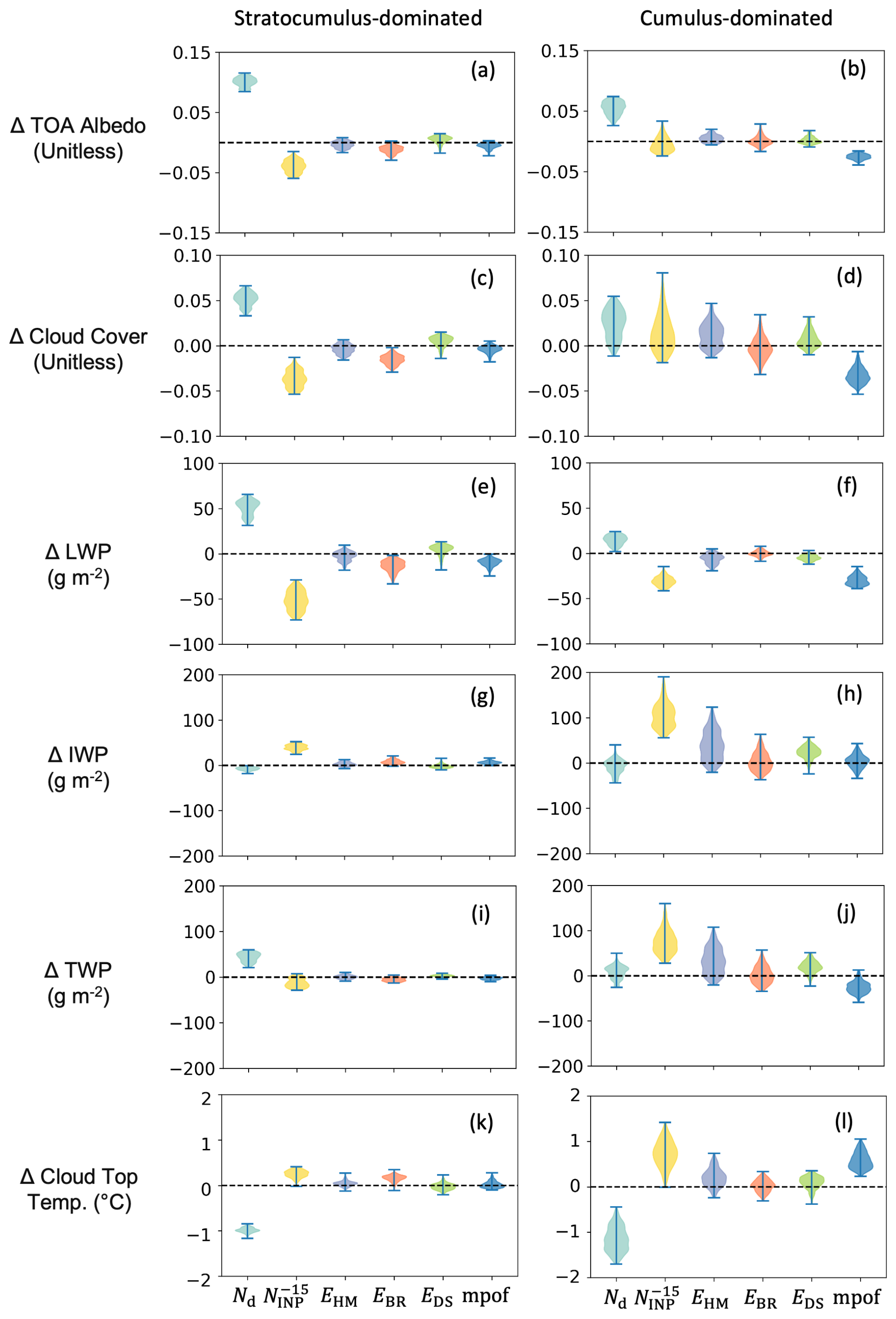
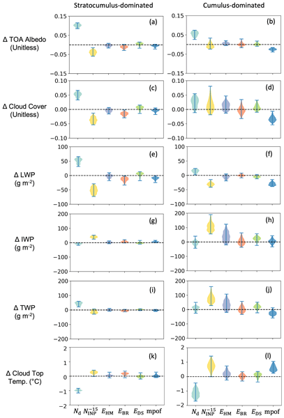
Figure 9 Distributions of the cloud property changes resulting from an increase of individual parameters one-at-a-time (OAT) in multiple OAT tests for: all-sky TOA albedo (a, b), cloud cover (c, d), all-sky LWP (e, f), all-sky IWP (g, h), all-sky TWP (i, j) and cloud top temperature (. The left panel shows the results from the Sc region, and the right panel shows the results from the Cu region. Errors of the GP model are propagated through into these multiple OAT test results, but the errors are generally much smaller than the variations shown here (Appendix C). For the process of performing the multiple OAT test, please refer to the details in Sect. 3.3.

We performed a large number OAT tests using the trained GP emulators for each model variable with different starting points. To design the starting points, three values were selected for each parameter: low (25 % of the perturbed range), mid (50 % of the perturbed range), and high (75 % of the perturbed range). For N parameters each with M values, the number of possible parameter combinations are M^N. Hence, there were 729 starting points (control sets of parameter values) across the 6-D parameter space in the multiple OAT tests. For each OAT test, the parameters were perturbed to the high-end (95 % of the perturbed range) and the low-end (5 % of the perturbed range) individually. The responses of cloud properties were the change from high-end parameter value output to the low-end parameter value output. The perturbed ranges in the multiple OAT tests were smaller than the perturbed parameter range in the PPE design to avoid the high uncertainties of emulators near boundaries of the parameter space. As for each parameter, we perturbed the value from low-end to high-end without directly including the emulator output from the control simulation, the number of output points from the emulator for each variable is $\mathrm{2}\times M^{N-\mathrm{1}}$. Therefore, for each model variable in one domain (one subplot in Fig. 9), the total number of investigated model variants is 2916. A compact distribution in Fig. 9 means that the sensitivity of the cloud property to that parameter is not strongly dependent on the setting of the other parameters.

The magnitudes of cloud responses to individual parameter perturbations are sometimes strongly dependent on the values of other parameters. For example, in the Sc region, the increase in LWP (Fig. 9e) by perturbing N_d from low to high values ranges from +31 to +65 g m⁻², and the decrease in LWP by perturbing $N_{\text{INP}}^{-\mathrm{15}}$ from low to high values ranges from −73 to −29 g m⁻². In the Cu region, the decrease in LWP (Fig. 9f) by perturbing mpof from low to high values ranges from −39 to −15 g m⁻². Although the projection plots suggest clouds are not very sensitive to variations of SIP processes, the multiple OAT tests here show that in some parameter space, varying SIP processes can have same or even stronger effects on cloud cover, IWP and TWP in the Cu region than N_d and $N_{\text{INP}}^{-\mathrm{15}}$. In addition, due to the existence of dominant parameters across the parameter space (e.g. N_d), the effects from SIP processes may be obscured through averaging in the paired projections. The relative importance of each parameter across the parameter space can also be quantitively compared by using the statistics of the sensitivities from the multiple OAT test (e.g. mean or mode), which shows similar results to those from a global sensitivity analysis in Appendix H. Similar to the other variables discussed above, parameter interactions are also identified here for CTT, particularly in the Cu region. Across different parts of the parameter space, an increase in N_d can reduce CTT from about −0.5 °C to nearly −2 °C in the Cu region. An increase in $N_{\text{INP}}^{-\mathrm{15}}$ can lead to an increase in CTT ranging from nearly 0 °C to about +1.5 °C. This dependence of individual parameter sensitivities on other parameters indicates that these parameters also jointly affect cloud vertical development in CAO clouds and may therefore influence cloud field evolution, such as the transition from stratocumulus to cumulus. It is therefore important to explore the full parameter space when assessing the effects of aerosols and ice-production processes on cloud evolution during CAO events.

The direction (or sign) of the cloud response can also depend on the control values of the parameters. For example, changes in SIP parameters in this case can cause either increases or decreases in cloud cover (Fig. 9c and d) depending on the other parameters (primarily N_d and $N_{\text{INP}}^{-\mathrm{15}}$ which dominate the sensitivities). In the Cu region, increasing $N_{\text{INP}}^{-\mathrm{15}}$ does not consistently lead to a reduction of the TOA albedo (Fig. 9b). For most OAT tests with $N_{\text{INP}}^{-\mathrm{15}}$ perturbations, increasing $N_{\text{INP}}^{-\mathrm{15}}$ causes cloud cover to increase (Fig. 9d), but also leads to a reduction in LWP (Fig. 9f). These two effects compensate each other for the effect of increasing $N_{\text{INP}}^{-\mathrm{15}}$ on TOA albedo. Therefore, the influence from a high $N_{\text{INP}}^{-\mathrm{15}}$ on TOA albedo in Cu region is controlled by multiple cloud properties, and these cloud properties can have different responses to changing $N_{\text{INP}}^{-\mathrm{15}}$ at different part of the parameter space.

In summary, the sensitivities of modelled cloud properties to each individual perturbed parameter depend on the starting point in the parameter space; this includes both the magnitudes and sign of responses. Results from our multiple OAT tests across the parameter space demonstrate that using a single OAT test is inadequate for determining the magnitude and even sign of the cloud response to model parameters. It is therefore important to investigate the whole parameter space for a more comprehensive understanding of the effects from these parameters.

4 Discussion and Conclusions

We present here the first analysis of mixed-phase CAO (cold-air outbreak) cloud responses to combinations of six key cloud microphysics parameters related to aerosol-cloud interactions and ice formation processes. The perturbed ranges of these parameters either match the observed ranges when available, or were chosen based on uncertain ranges suggested by previous studies. The full 6-dimensional parameter space of cloud responses was explored using PPEs (perturbed parameter ensembles), GP (Gaussian Process) emulators, and multiple OAT (one-at-a-time) tests across the whole parameter space. The properties we investigated included all-sky TOA (top-of-the-atmosphere) albedo, all-sky LWP (liquid water path), cloud cover, all-sky IWP (ice water path), and all-sky TWP (total water path) which are key properties that influence the radiative effects of mixed-phase clouds (Ceppi et al., 2017). Model simulations were based on a CAO event case over the Labrador Sea on 24 October 2024, focused on Sc (stratocumulus) and Cu (cumulus) cloud regimes and covering the routes of two research flights from the M-Phase aircraft campaign (Murray and the M-Phase Team, 2024; Clarke et al., 2026).

In this CAO case, where the liquid phase dominates with cloud top temperatures of around −15 °C, N_d exerts the strongest controls on TOA albedo and LWP in both regions with the Twomey effect (Twomey, 1977) and the Albrecht effect (Albrecht, 1989). The effects of N_d on mixed-phase CAO clouds in these simulations are also consistent with previous simulations from de Roode et al. (2019) who reported that higher N_d leads to a higher LWP and cloud cover, and vice versa. However, we further show that the effect of changing N_d varies strongly across the parameter space. Perturbing N_d from low to high in different parts of the parameter space leads to TOA albedo responses ranging from +0.08 to +0.11 and LWP responses ranging from +31 to +65 g m⁻² in the Sc region, and TOA albedo responses ranging from +0.02 to +0.07 and LWP responses ranging from near-zero (+2 g m⁻²) to +24 g m⁻² in the Cu region. Thus, although the effect of N_d on albedo and LWP are dominating, there are strong variations depending on other parameters. Such variation demonstrates the importance of performing simulations across a joint parameter space to avoid incomplete conclusions or overly confident estimates of sensitivities.

An increase in $N_{\text{INP}}^{-\mathrm{15}}$ leads to a reduction in TOA albedo and LWP in the Sc region in this case, which is consistent with the results from previous studies on the influences of different INP concentrations (Tornow et al., 2021) or ice treatment in models (Abel et al., 2017). However, the sampling of parameter space using PPEs and emulators shows that the magnitude and even sign of response to $N_{\text{INP}}^{-\mathrm{15}}$ perturbations depends on the setting of other parameters, even within the single environment represented by the case we studied. It is seen in the Sc region that the modelled TOA albedo is not sensitive to $N_{\text{INP}}^{-\mathrm{15}}$ when N_d is low (less than approximately 20 cm⁻³). A similar weak sensitivity of clouds to changes in $N_{\text{INP}}^{-\mathrm{15}}$ was found by the study from McCluskey et al. (2024) over the Southern Ocean, where they found that the modelled IWP was relatively insensitive to the representation of INP under low N_d condition. It is shown that their model underestimates CCN concentration (Niu et al., 2025) over the Southern Ocean, which could account for the weak INP sensitivity consistent with our results. We also find that in the Cu region, the sensitivity of clouds to $N_{\text{INP}}^{-\mathrm{15}}$ is relatively weaker and the sign of the cloud response as a function of $N_{\text{INP}}^{-\mathrm{15}}$ varies over the parameter space. For example, an increase in $N_{\text{INP}}^{-\mathrm{15}}$ can lead to both increases and decreases of TOA albedo (from −0.02 to +0.03) and cloud cover (from −0.02 to +0.08) when the values of other parameters are changed. The pronounced variation in the modelled cloud sensitivity to INP concentrations highlights the importance of having good representations of other microphysical processes in the model and the necessity of a full exploration of the parameter space, including other cases, to understand the role of INPs in mixed-phase CAO clouds.

Our results show that, for this CAO case, N_d and N_INP strongly control the radiative properties of mixed-phase clouds in the Sc region, but with large uncertainty in the sensitivities depending on other poorly quantified model parameters. The strong sensitivity of this CAO case to changes in N_d highlights the importance of accurately representing and treating CCN in models in order to better simulate mixed-phase CAO clouds. Our results also show that cloud sensitivities to N_d can depend on N_INP. Because measurements of INP concentrations are sparse and cannot be obtained from satellite retrievals or other remote-sensing observations, the sensitivity of clouds to CCN can remain difficult to constrain without knowing INP concentrations. Improved temporal and spatial coverage of INP measurements is therefore also needed to better constrain the properties and sensitivities of mixed-phase CAO clouds, together with improved representation of INPs in atmospheric and climate models.

The SIP parameters generally have a weak effect on the radiative properties (TOA albedo) of the studied CAO clouds. Our results on the effect from SIP processes on LWP are generally consistent with previous work from Karalis et al. (2022) who showed that an enhancement of SIP can lead to the reduction of LWP. However, we show that the magnitude of LWP (and other cloud properties) responses to perturbations of all three SIP parameters vary across the parameter space, with strong dependency on the other parameters such as N_d and $N_{\text{INP}}^{-\mathrm{15}}$. Compared to the results from Karalis et al. (2022), the relative importance of each of the SIP processes differs between our study and theirs. In Karalis et al. (2022), the droplet shattering process was more effective than the Hallett–Mossop process in the Cu region, while the Hallett–Mossop process exerts stronger effects on LWP in our case. Such differences may occur because the environmental conditions vary between cases, which will affect the efficiencies of SIP processes. In addition, Karalis et al. (2022) used alternative parameterisations for the droplet-shattering and ice-ice breakup processes which follow Phillips et al. (2017). Therefore, it is worth noting that our conclusions are potentially specific to this CAO case and may be dependent on the CAO case being simulated, and may be influenced by the model setup or choice of parameterisations.

Opposite responses of TWP to stronger ice formation processes (e.g. a higher $N_{\text{INP}}^{-\mathrm{15}}$ or E_HM) are seen in the two regions, with strong variations of TWP responses in the Cu region. Stronger ice formation reduces TWP in the Sc region but increases TWP in the Cu region. Wu et al. (2025) similarly showed that a simulation with a high ice number concentration produced a higher TWP than one with a low ice number concentration approximately 15 h after the ice edge, although the simulation with the lowest ice number concentration produced the highest TWP at earlier stages. Lee et al. (2021) focused on mid-latitude mixed-phase stratocumulus and also found that increasing INP concentrations enhanced depositional growth and increased TWP. Our IWP and LWP responses to a higher ice number concentration in the Sc region are also comparable to those reported by Tornow et al. (2021). However, the IWP in their Cu region was much less sensitive to ice number concentration than that found in our study. Juliano et al. (2026) showed that models exhibit diverse LWP and IWP responses when switching from liquid-only to mixed-phase configurations. We therefore suggest that differences in the parameterisation and treatment of cloud processes among models may contribute to their differing sensitivities of cloud water paths to ice formation. Given that the TWP response to ice formation processes differs even between regions within the same case examined here, we expect the balance among processes to be both case- and regime-dependent. The positive TWP response identified in this study should therefore not be interpreted as a universal response to increased ice formation.

The influence of the mixed-phase overlap factor (mpof) in this case is more prominent in the Cu region where an increase in mpof leads to a reduction in LWP and cloud cover, and therefore a lower TOA albedo. These responses of cloud properties to changes in the mpof value are similar to the results from Abel et al. (2017). However, the sensitivity of LWP as a function of mpof in our work is weaker in the Sc region than seen in Abel et al. (2017) where they also modified the cloud liquid and ice overlap. Although our case here has similar cloud temperature as the case investigated in Abel et al. (2017), the overlap parameter used in their work is from the bulk cloud scheme, while the mpof in our work is within the cloud microphysics scheme. This suggests that different model setups can also lead to potentially different sensitivities of cloud properties to the parameters. Similar to the other parameters, the effect from mpof on the investigated cloud properties vary across the parameter space and interactively affect the influence of the other parameters.

We expect the large, non-linear joint effects of cloud microphysical parameters on CAO clouds will be a feature of CAOs in other meteorological environments, but the sensitivities are likely to vary. By limiting our analysis to a single case study, we are able to fully explore the sensitivity of the CAO clouds to six key parameters without the confounding effects of environmental conditions. The sensitivity of mixed-phase CAO clouds to the parameters investigated here may be substantially different in a different CAO event. For example, in previous work we showed that the sensitivities of mixed-phase CAO clouds to INP concentration can differ in magnitude and sign between warm and cold cases (Huang et al., 2025). Previous studies have shown that CAO cloud properties depend strongly on environmental conditions (Fletcher et al., 2016b; McCoy et al., 2017; Wu and Ovchinnikov, 2022; Murray-Watson et al., 2023), including factors such as CAO strength and wind conditions. This environmental dependence is likely to modify CAO cloud sensitivities to the parameters examined here. Future work should therefore investigate how different environmental conditions influence CAO clouds and how those influences interact with key cloud microphysical parameters.

In this first PPE study of a high-resolution regional model of mixed-phase clouds, we have made several simplifying assumptions in the cloud microphysics processes, including the use of fixed N_d and temperature-dependent N_INP, rather than aerosol-interactive CCN and INP. This choice was made to reduce the complexity of the model result interpretation and to have a direct understanding of N_d and N_INP interactions which is the main objective of this study. However, this approach omits several potentially important processes, including interactions of aerosols and cloud hydrometeors, feedbacks associated with aerosol and in-cloud processing of CCN and INP, and the influence of different aerosol sources. These processes could alter the sensitivities of CAO clouds to aerosols and to other microphysical parameters. Future work should therefore include aerosol-interactive CCN and INP in order to provide a more complete representation of aerosol effects and their interactions in mixed-phase CAO clouds. In addition, our analysis does not include all potentially important parameters and processes, such as boundary-layer mixing (Field et al., 2014) and cloud fraction schemes (cloud macrophysics) (Van Weverberg et al., 2023). Future studies should extend the analysis to include these additional parameters in order to provide a more comprehensive quantification of uncertainty in CAO cloud properties.

To conclude, this work illustrates the power of using PPEs and model emulation for systematically identifying important non-linear joint effects of multiple cloud microphysical parameters on mixed-phase CAO clouds. These interactions of parameters cannot be revealed using single OAT tests, which may therefore lead to misleading or overly confident estimates of the key factors controlling mixed-phase CAO cloud properties. Exploration of the entire parameter space is necessary to fully understand the influences on CAO clouds from these uncertain model parameters, and to constrain the effect of the uncertainties on the estimation of cloud-phase feedback.

Appendix A: Deriving a new n_s(T) parameterisation for soil dusts

A recent study by Herbert et al. (2025) has shown that the ice-nucleating ability of dust in the atmosphere is influenced by a mineral component and a biogenic component associated with the surface area of the dust. The authors suggest that soil dusts that have come from arid, desert-like, environments are best represented by the mineral component alone, whereas dusts from biologically productive regions are best represented by the inclusion of both components. The authors refer to these two classes of soil dusts as desert soils and fertile soils, respectively. Some parameterisations that are commonly used to represent INP concentrations in modelling studies (Harrison et al., 2019, e.g.) only account for the mineral component, and therefore may only be representative of desert soils. Here, we present a new empirical parameterisation for the ice-nucleating activity of fertile soils, which is likely more representative of INP measurements in the mid- to high latitudes (Herbert et al., 2025).

Laboratory measurements of soil-dust ice nucleating activities were collated from literature (Barr et al., 2023; King, 2024; O'Sullivan et al., 2014; Paramonov et al., 2018; Porter et al., 2020; Sanchez-Marroquin et al., 2020; Thompson, 2024; Steinke et al., 2016, 2020). These are studies that have tested the untreated properties of soil dusts that have been sampled in situ or collected from the surface. We purposefully omit measurements from desert soil sources, such as the Sahara desert.

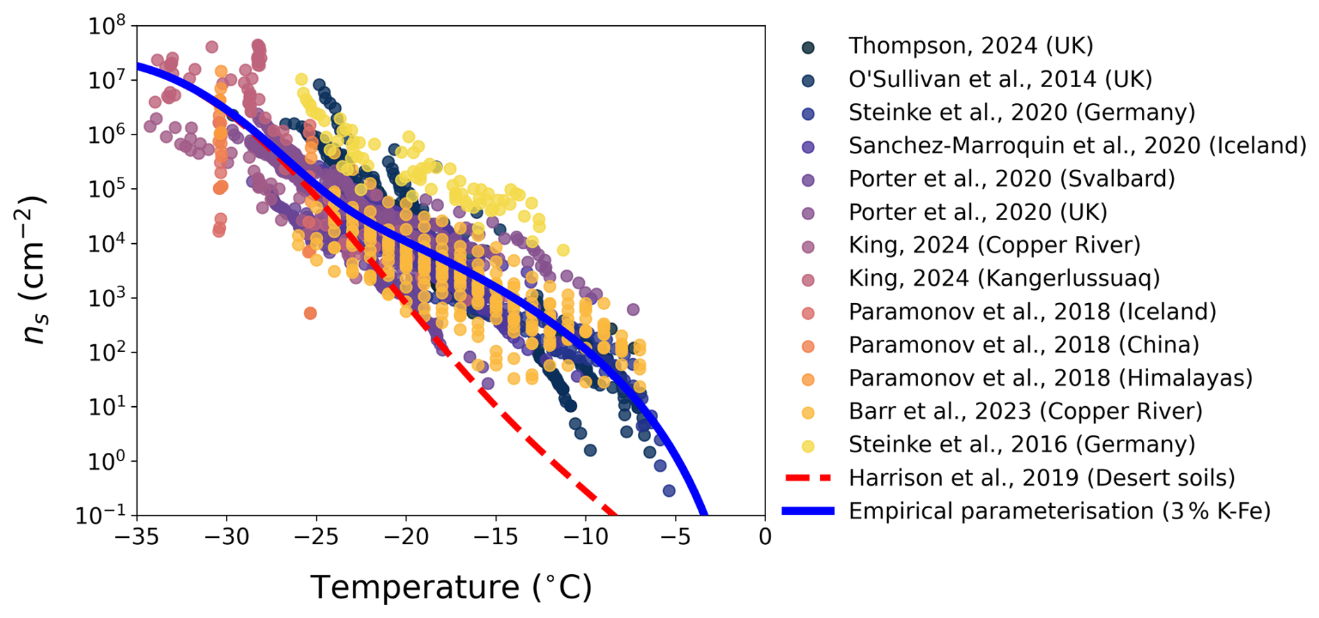
Figure A1 Empirical soil-dust parameterisation of n_s,soil(T). Coloured circles show measurements from laboratory studies (references within figure) that have measured the ice-nucleating activity of soil dust sampled from locations around the world. The red dashed line shows the parameterisation for desert soils from Harrison et al. (2019), whilst the solid blue line shows the best fit to the data assuming a K-Fe component (weight percent of 3 %) and a biogenic component described by a power law.

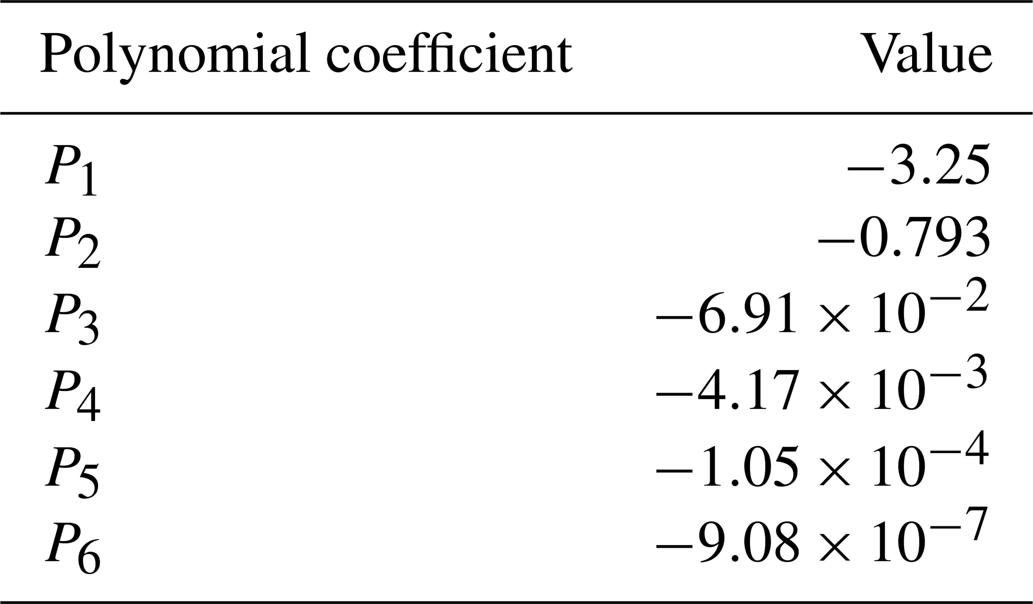
We use the measurements to produce an empirical parameterisation which consists of two additive functions, accounting for the two components. For the mineral component, we use a parameterisation from Harrison et al. (2019) that is dependent on the potassium-feldspar (K-Fe) present in the dust (shown separately in Fig. A1). We use a constant K-Fe content (f_KFe) of 0.03, which is representative of a global-mean value (Harrison et al., 2019). For the biogenic component, we use the power law $n_{\mathrm{s}}\left(T\right)=-k{T}^{\mathit{\alpha }}$, which provides a shape consistent with measurements of n_s at high temperatures (Fig. A1). The variables α and k were systematically varied until the root-mean square error between the measurements and summed contributions of the two functions was minimized. The resulting parameterisation of n_s,soil(T) in cm⁻² is shown in Fig. A1, and described by the function

$$\begin{array}{ll}{\displaystyle }{n}_{\mathrm{s},\text{soil}}\left(T\right)=& {\displaystyle }(-k{T}^{\mathit{\alpha }})\\ \text{(A1)}& {\displaystyle }& {\displaystyle }+{\mathrm{10}}^{(P_{\mathrm{1}}+P_{\mathrm{2}}T+P_{\mathrm{3}}{T}^{\mathrm{2}}+P_{\mathrm{4}}{T}^{\mathrm{3}}+P_{\mathrm{5}}{T}^{\mathrm{4}}+P_{\mathrm{6}}{T}^{\mathrm{5}})}{f}_{\text{KFe}},\end{array}$$

where $k=\mathrm{3.907}\times {\mathrm{10}}^{-\mathrm{5}}$, α=6.531, and the values of P₁ to P₆ are shown in Table A1. The temperature T is in °C.

Table A1 Polynomial coefficients used in Eq. (A1). Values are taken from Harrison et al. (2019)

Appendix B: Simulated aerosol size distributions during M-Phase

In this section, we produce an INP parameterisation that is representative of the location and time period of the M-Phase campaign. We apply the new n_s,soil(T) parameterisation from Eq. (A1) to simulated dust concentrations and the marine INP parameterisation (n_s,SSA(T)) from McCluskey et al. (2018) to simulated sea-spray aerosol (SSA) concentrations. The concentrations are simulated using a global configuration of the Met Office Unified Model (Brown et al., 2012a) version 12.1 which includes Global Atmosphere version 8.0 and Global Land model version 9.0 (Willett et al., 2026). The configuration we use is described in detail by Jones et al. (2022) with the addition of dust in a super-coarse aerosol mode. The emission, advection, and removal of aerosol is simulated by the UK Chemistry and Aerosol (UKCA-mode) model (Mann et al., 2010) which includes a prognostic two-moment aerosol microphysics scheme. In this configuration of UKCA-mode, aerosol components (SSA, sulphate, black carbon, organic carbon, and dust) are represented by log-normally distributed aerosol modes. SSA is present in the accumulation and coarse modes. Dust is present in the accumulation, coarse, and super-coarse modes. Global dust emission parameters (horiz_d, us_am, and sm_corr) were tuned to global observations of dust aerosol optical depths, dust size distributions, surface dust concentrations, and dust deposition fluxes (Woodward et al., 2022). The resulting values are horiz_d=6.0, us_am=1.45, and sm_corr=0.7.

A simulation was run from 2018 to 2024, with U and V wind components above the boundary layer nudged to 6-hourly ERA5 reanalysis, and sea surface properties and fluxes represented by observed climatologies of sea surface temperature and sea ice content. The simulated SSA and dust aerosol size distributions were extracted for a region (62.8–51.6° W, 53.1–60.6° N) and time period (23 October–5 November 2022) consistent with the M-Phase campaign. The INP number concentration (N_INP) is calculated at each temperature T and in each aerosol size bin i following the singular description (Murray et al., 2012; DeMott et al., 2015; Vali, 2008) using

$$\begin{array}{ll}{\displaystyle }{N}_{{\text{INP}}_{\mathrm{i}}}\left(T\right)=& {\displaystyle }{N}_{{\text{dust}}_{\mathrm{i}}}\left(\mathrm{1}-{\mathrm{e}}^{n_{\mathrm{s},\text{soil}}\left(T\right)\mathit{\pi }{d}^{\mathrm{2}}}\right)\\ \text{(B1)}& {\displaystyle }& {\displaystyle }+N_{{\text{SSA}}_{\mathrm{i}}}\left(\mathrm{1}-{\mathrm{e}}^{n_{\mathrm{s},\text{SSA}}\left(T\right)\mathit{\pi }{d}^{\mathrm{2}}}\right),\end{array}$$

where $N_{{\text{dust}}_{\mathrm{i}}}$ and $N_{{\text{SSA}}_{\mathrm{i}}}$ are the dust and SSA number concentrations in each size bin (L⁻¹ of air) and d is the mean diameter of the bin. The bins are summed to obtain the total N_INP for each grid box and for each time step (3 h) of the time series. This is repeated for three model levels (surface, 1 and 2 km) and a mean taken over the three to provide a concentration that is representative of the vertical cloud structure in the region (92 % of Sc clouds and 70 % of Cu clouds are below 2 km). A polynomial fit to all values of N_INP is used to produce a parameterisation for N_INP,M-Phase(T) which is described by

$$\begin{array}{ll}{\displaystyle }& {\displaystyle }{\log }_{\mathrm{10}}{N}_{\text{INP,M-Phase}}\left(T\right)=-\mathrm{4.591}-\mathrm{0.5284}T\\ {\displaystyle }& {\displaystyle }-\mathrm{3.341}\times {\mathrm{10}}^{-\mathrm{2}}{T}^{\mathrm{2}}-\mathrm{1.249}\times {\mathrm{10}}^{-\mathrm{3}}{T}^{\mathrm{3}}\\ \text{(B2)}& {\displaystyle }& {\displaystyle }-\mathrm{1.579}\times {\mathrm{10}}^{-\mathrm{5}}{T}^{\mathrm{4}},\end{array}$$

where N_INP,M-Phase has units L⁻¹ of air and T is in °C.

The regional model and global model were performed separately, and the use of the global model was solely for providing a temperature-dependent INP parameterisation (Eq. B2).

Appendix C: Kernel selection and evaluation of GP emulators

In this section, we present the results of GP kernel selection and emulator evaluation. We evaluated four stationary kernels using cross-validation on the 66-member training set. In each cross-validation set, 60 points were used for training and 6 for testing. We selected the kernel with the lowest RMSE for each variable, retrained the emulator using all 66 training points, and then evaluated it with an independent 6-member test set generated by Latin hypercube sampling.

Figures C1–C4 show the standardized error, $\frac{Y_{\text{pred}}-Y_{\text{true}}}{{\mathit{\sigma }}_{\text{emulator}}}$, together with Q–Q plots, RMSE, and R². For most cloud variables, the Matérn32 kernel produced the lowest RMSE and was therefore selected. The two exceptions are total water path in the Sc region, for which the RBF kernel performed best, and ice water path in the Cu region, for which the Matérn12 kernel performed best. However, the differences in RMSE relative to the Matérn32 kernel are small in both cases.

All predictions for the testing points have 95 % confidence intervals (2σ) that are across the 1:1 line, satisfying the validation criterion suggested from Bastos and O'Hagan (2009). We also compared the standard deviation of the test data with the mean standard deviation from emulators across the test points. For all variables, the standard deviation of the test data is higher than the mean standard deviation from emulators across the test points, indicating that the emulators are able to capture the responses and variations of these variables to the perturbations of parameters.

The RMSE values are generally much smaller than the spread of the test data, the 1 million model variants shown in Fig. 6, and the variations from the multiple OAT tests shown in Fig. 9. This indicates that the emulators are sufficiently accurate for identifying interactions among the perturbed parameters. However, for ice water path in both regions and total water path in the Cu region, the emulator performance is less satisfactory than the others. This may come from multiple ice production processes interacting and dominating these variables, and hence lead to a greater complexity. Future work is recommended to investigate on the improvement of emulator performance (e.g. testing with different kernels) for these variables, particularly in the Cu region.

To assess whether 66 training points are sufficient, we performed a convergence test (Fig. C5) using different training sizes (N), with data sampled from the existing 66 training points. For each size with N<66, we randomly selected N training points 30 times and evaluated the emulator against the 6-member test set. The RMSE values for N=66 are identical to those shown in Figs. C1–C4. For most variables, RMSE decreases rapidly up to about 54–60 training points and remains relatively stable thereafter. This suggests that adding simulations beyond 60 will only have small improvements in emulator performance, while requiring substantial additional computational cost. The spread of RMSE across the 30 random subsamples generally decreases as the number of training points increases, and is smallest at 65 training points. This is consistent with the use of the Latin hypercube sampling method, which was designed for an efficient coverage of the multi-dimensional parameter space.

A more standard convergence test is to compare emulators trained on multiple PPEs of different sizes, each generated independently with the Latin hypercube sampling method. However, such test is not feasible here because of the high computational cost of each simulation in our model setup. Future work with a cheaper model setup (e.g. a smaller domain) is recommended to investigate the number of points needed for robust emulator performance using this approach.

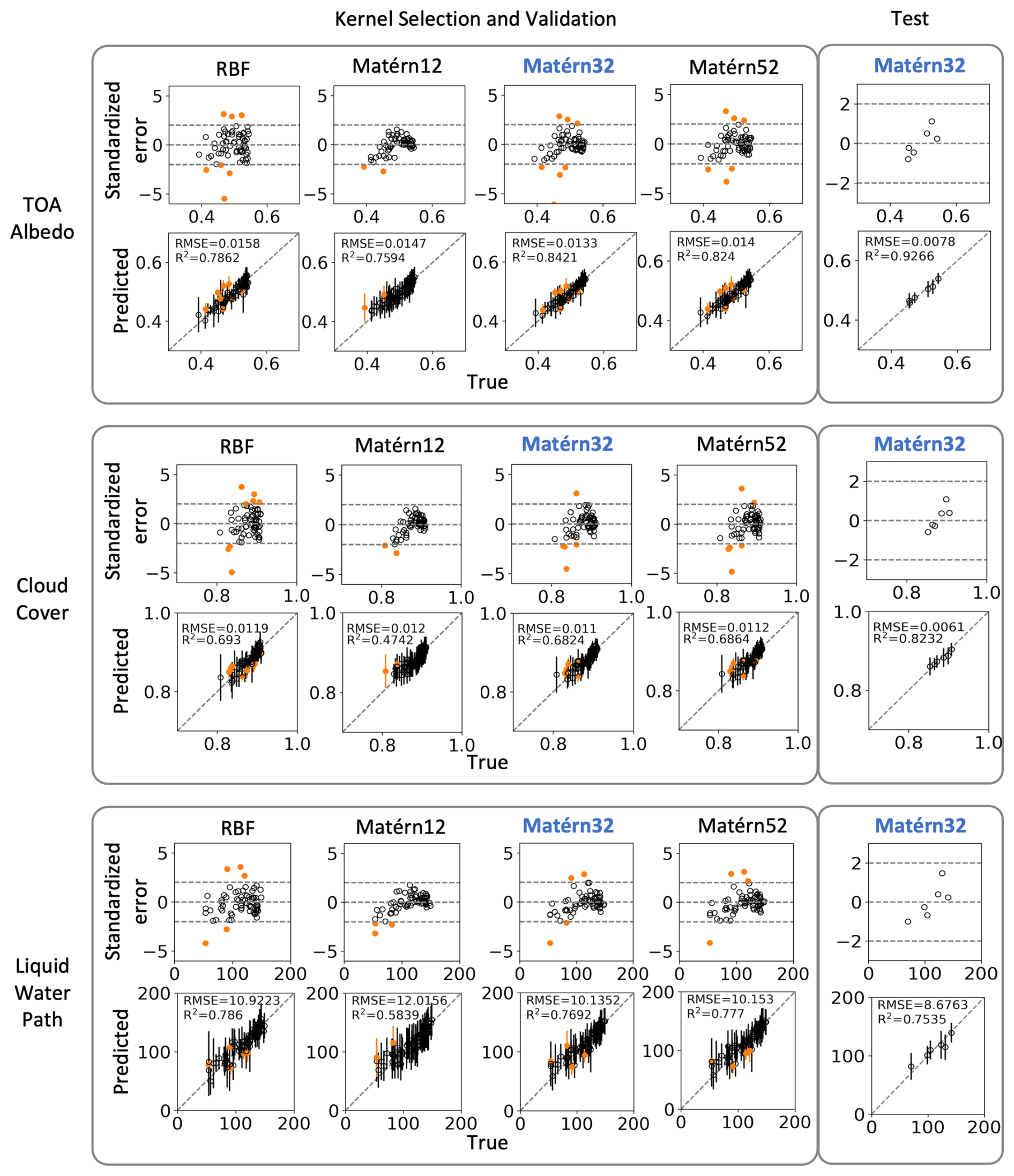
Figure C1 Kernel selection and testing results of the GP emulators on TOA albedo, cloud cover, and LWP in the Sc model analysis region. Points in orange indicate a failed emulated point in the standardized error check. The kernel name highlighted in blue indicates that the kernel was selected and the testing results are from comparing the emulator trained with the selected kernel with the testing dataset.

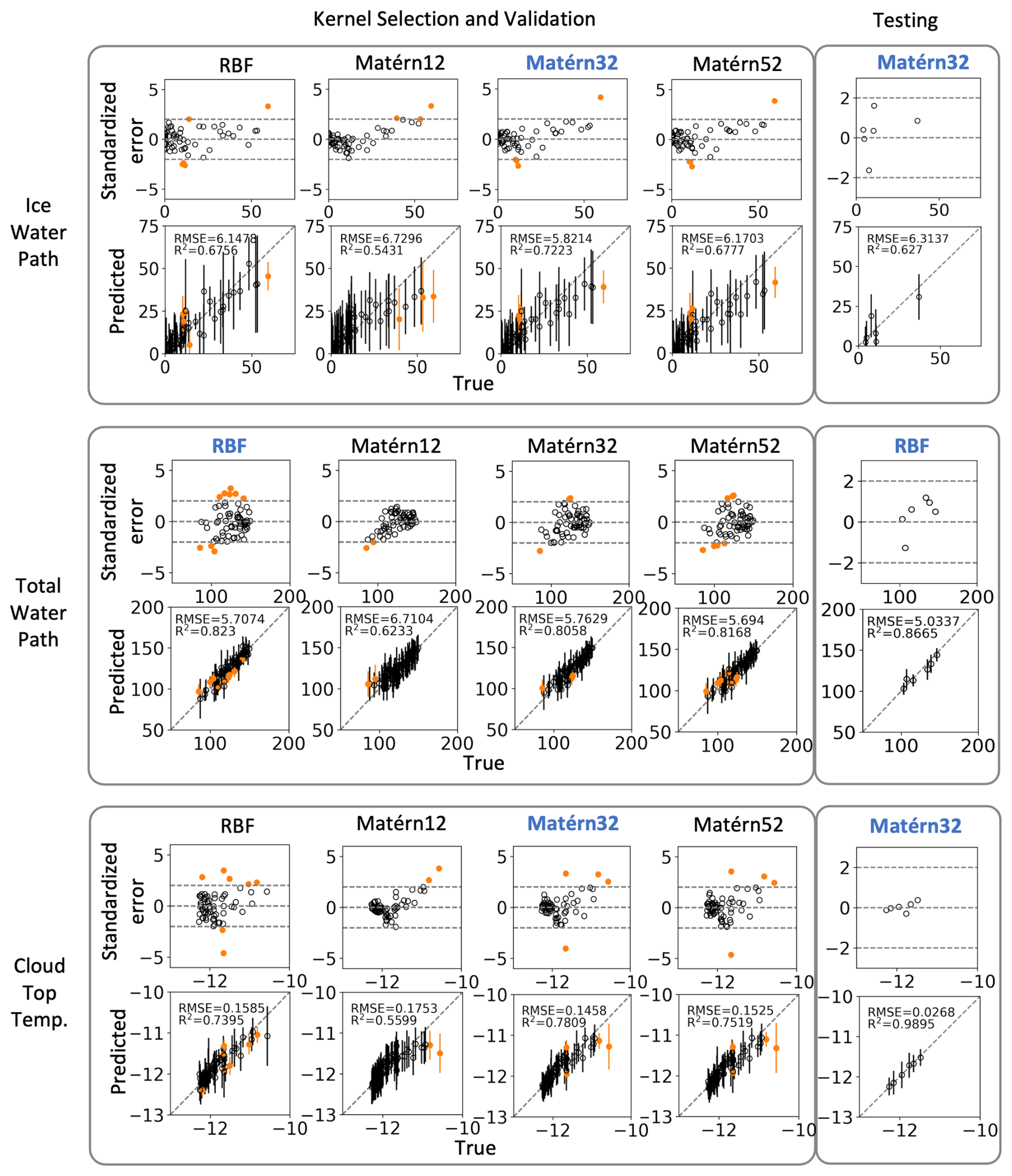
Figure C2 Kernel selection and testing results of the GP emulators on IWP, TWP, and cloud top temperature in the Sc model analysis region. Points in orange indicate a failed emulated point in the standardized error check. The kernel name highlighted in blue indicates that the kernel was selected and the testing results are from comparing the emulator trained with the selected kernel with the testing dataset.

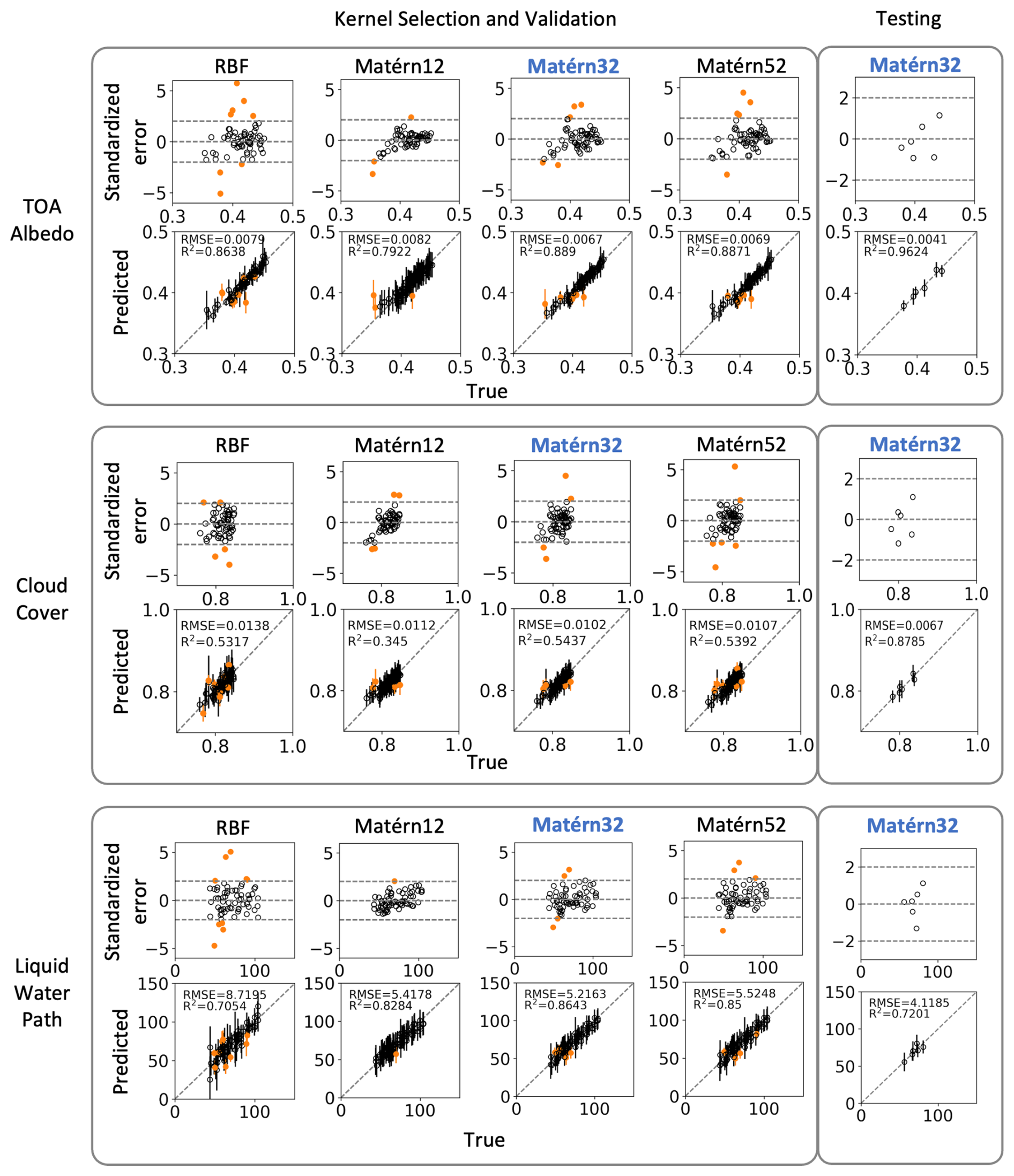
Figure C3 Kernel selection and testing results of the GP emulators on TOA albedo, cloud cover, and LWP in the Cu model analysis region. Points in orange indicate a failed emulated point in the standardized error check. The kernel name highlighted in blue indicates that the kernel was selected and the testing results are from comparing the emulator trained with the selected kernel with the testing dataset.

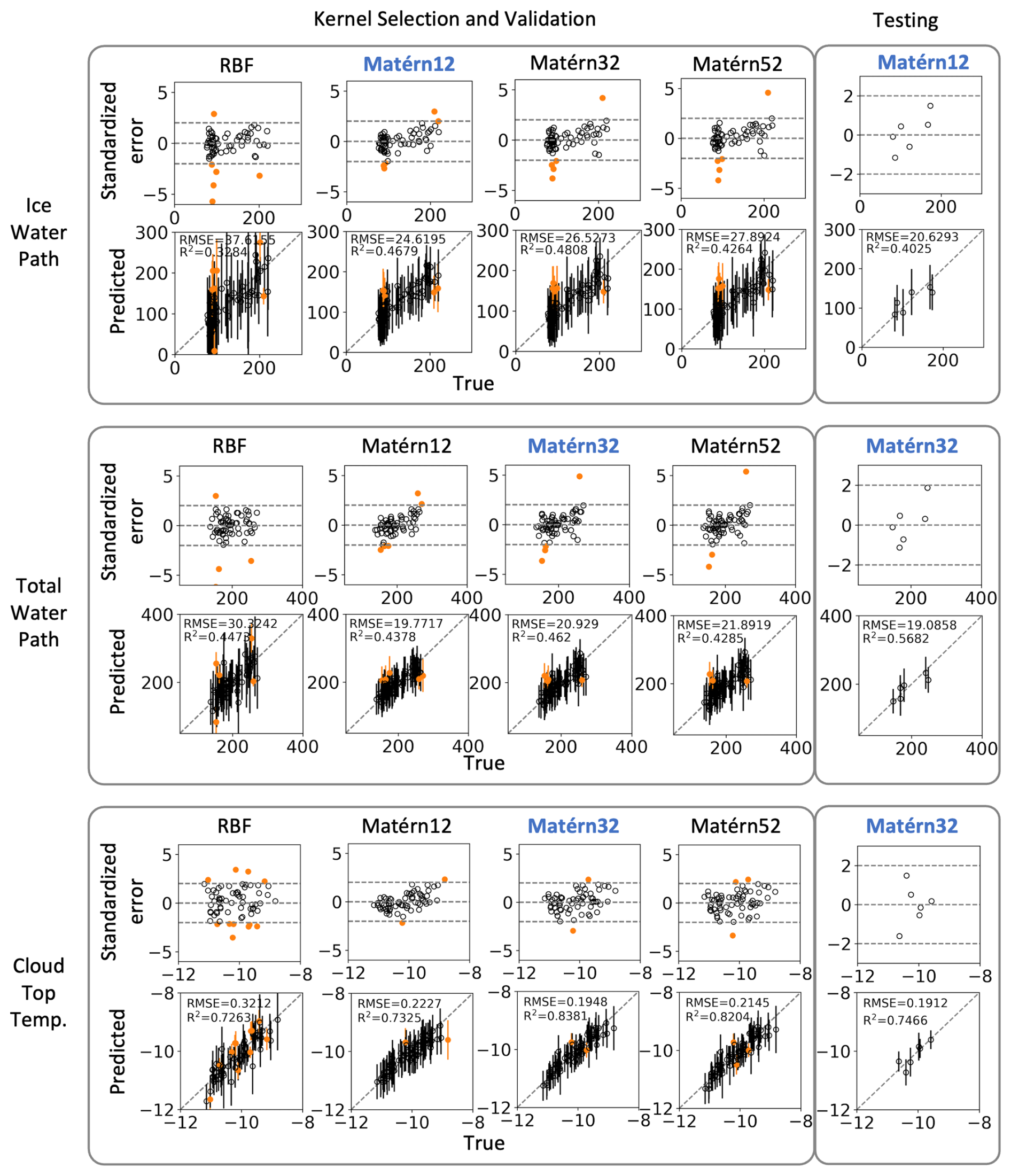
Figure C4 Kernel selection and testing results of the GP emulators on IWP, TWP, and cloud top temperature in the Cu model analysis region. Points in orange indicate a failed emulated point in the standardized error check. The kernel name highlighted in blue indicates that the kernel was selected and the testing results are from comparing the emulator trained with the selected kernel with the testing dataset.

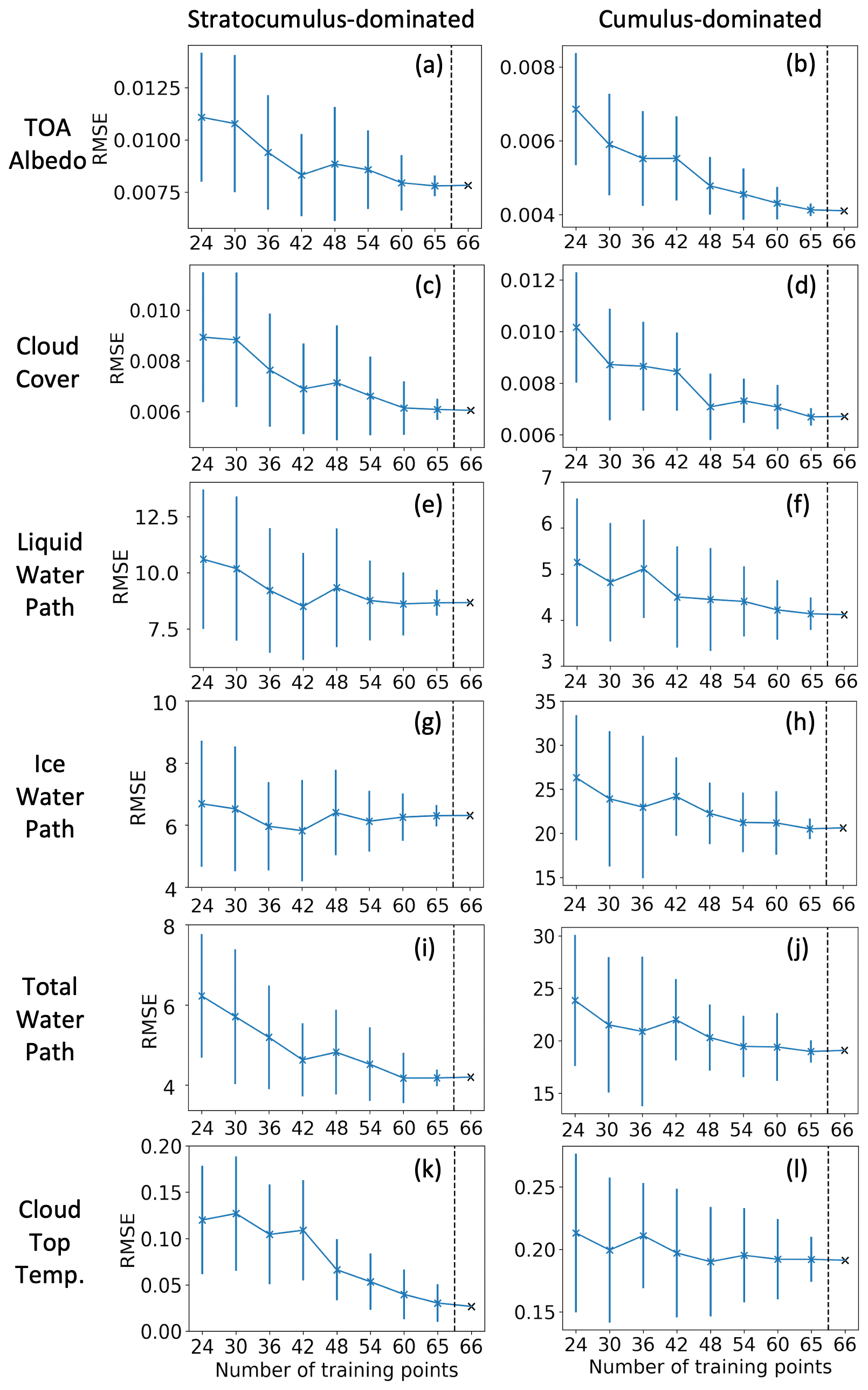
Figure C5 Convergence test results (RMSE) by using different number of training points over the Sc region (left) and the Cu region (right) for: (a, b) TOA albedo (unitless), (c, d) cloud cover (unitless), (e, f) liquid water path (gm⁻²), (g, h) ice water path (gm⁻²), (i, j) total water path (gm⁻²), and (k, l) cloud top temperature (°C).

Appendix D: Flow chart for methods involved in this work

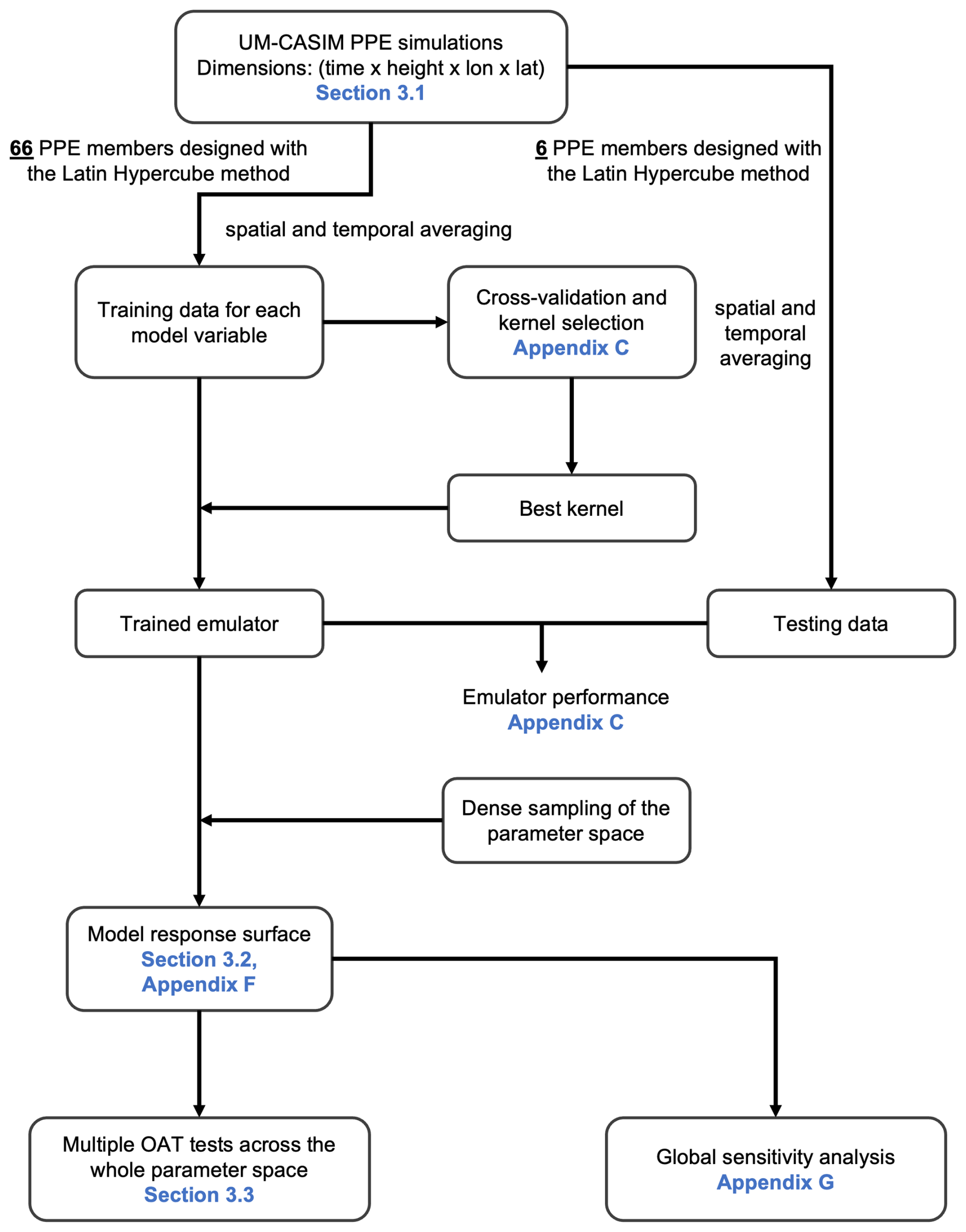
Figure D1 Flowchart for methods involved in this work. The sections include the corresponding results are highlighted in blue.

Appendix E: Simple illustration of linear and non-linear joint effects between two parameters

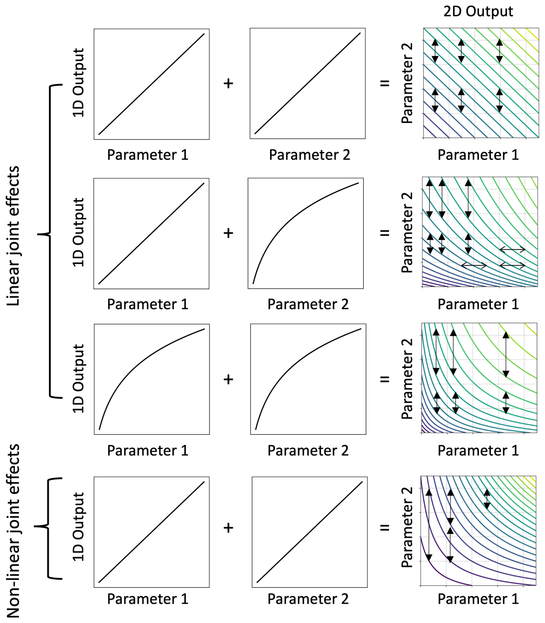
Figure E1 A simple illustration of linear and non-linear joint effects between two parameters. This diagram is adapted from Fig. 3.3 in the work of Sansom (2023). With linear joint effects, the effect of changing one parameter on the model output is independent of the value of the other parameter. With non-linear joint effects, the effect of changing one parameter on the model output is then dependent on the value of the other parameter. The length of the arrows shown in the 2D output represents the variation needed for a parameter to across three contour lines. All the contour lines shown here are with linear scale.

Appendix F: Additional paired-projection figures from GP emulators

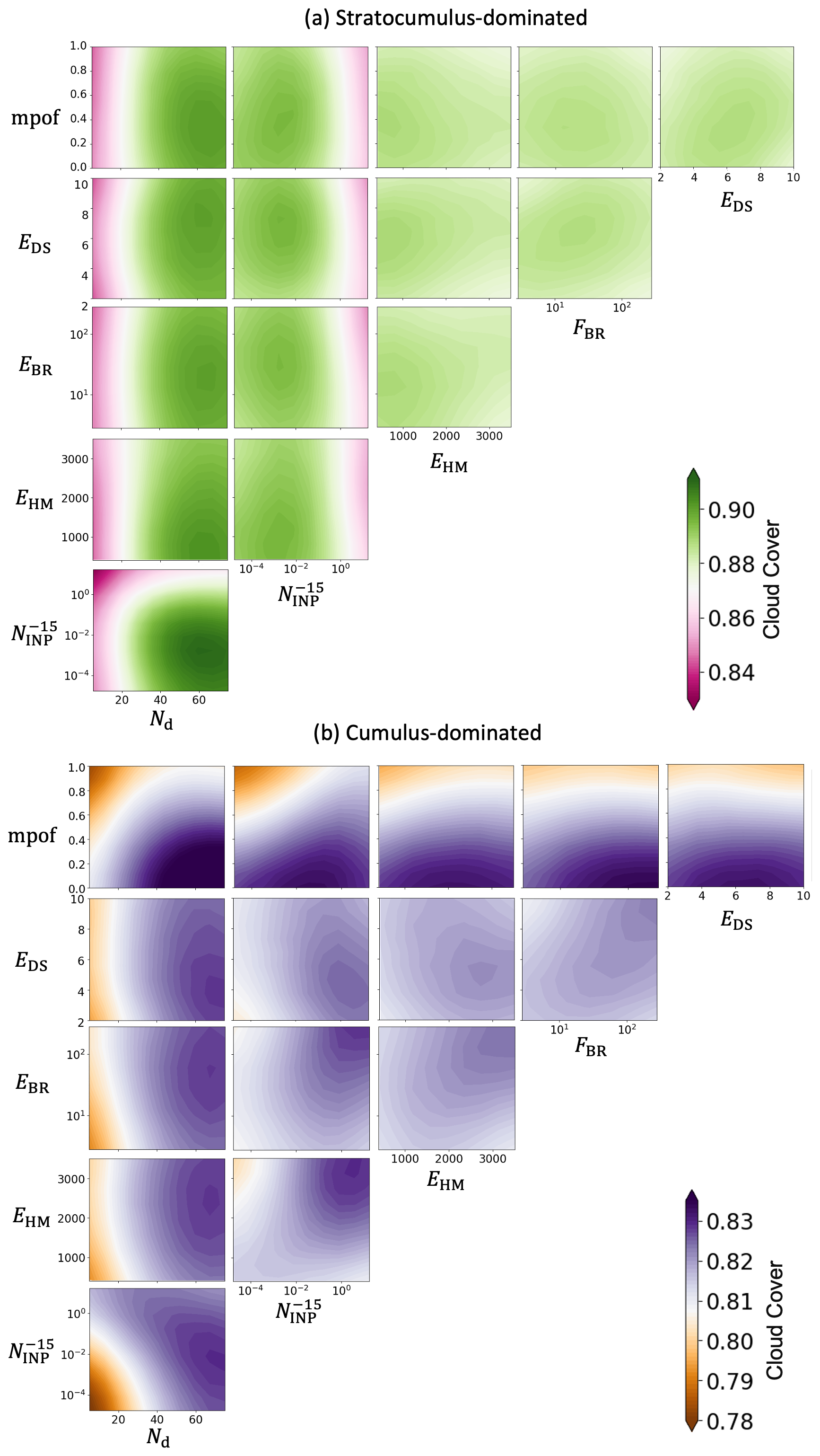
Figure F1 Projected mean model responses of cloud cover to paired parameters in (a) Sc region and (b) Cu region.

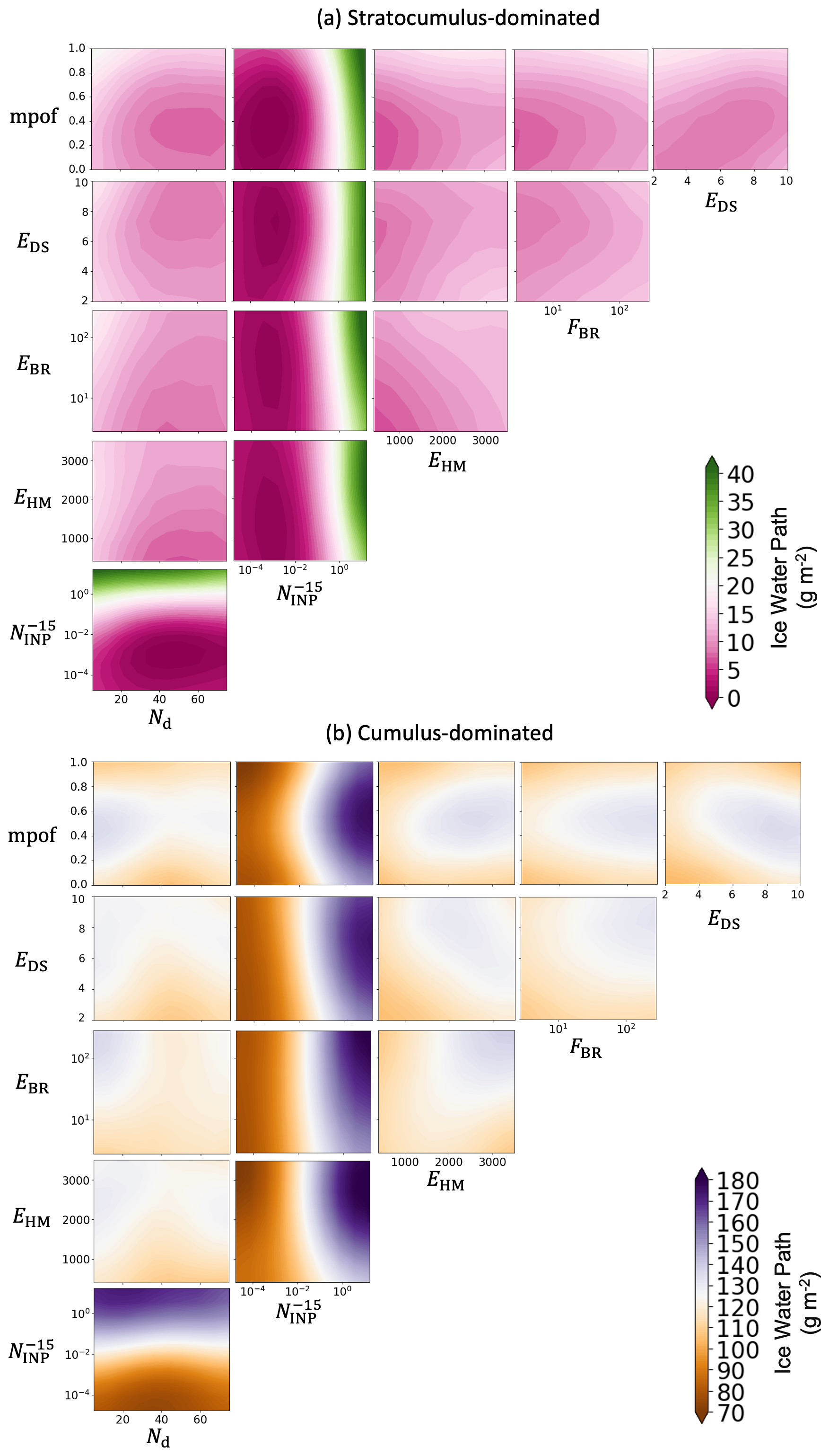
Figure F2 Projected mean model responses of all-sky IWP (ice water path) to paired parameters in (a) Sc region and (b) Cu region.

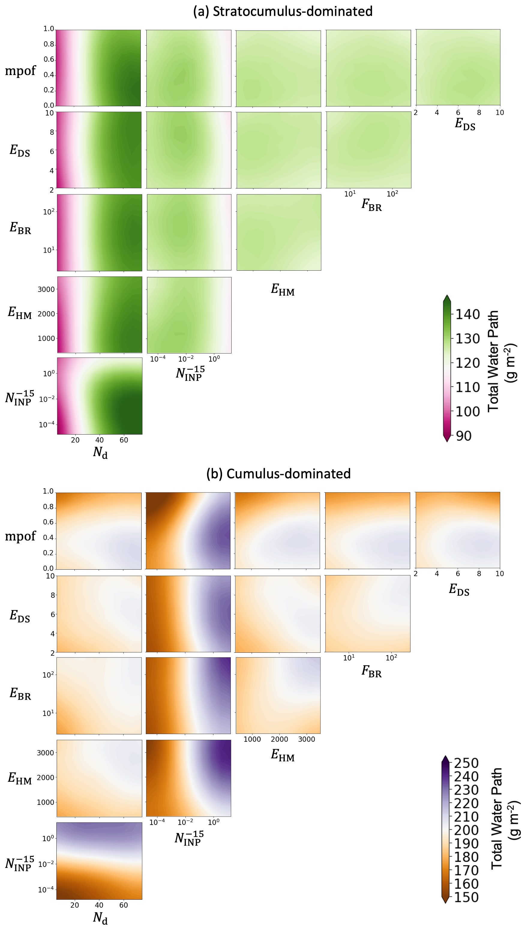
Figure F3 Projected mean model responses of all-sky TWP (total water path) to paired parameters in (a) Sc region and (b) Cu region.

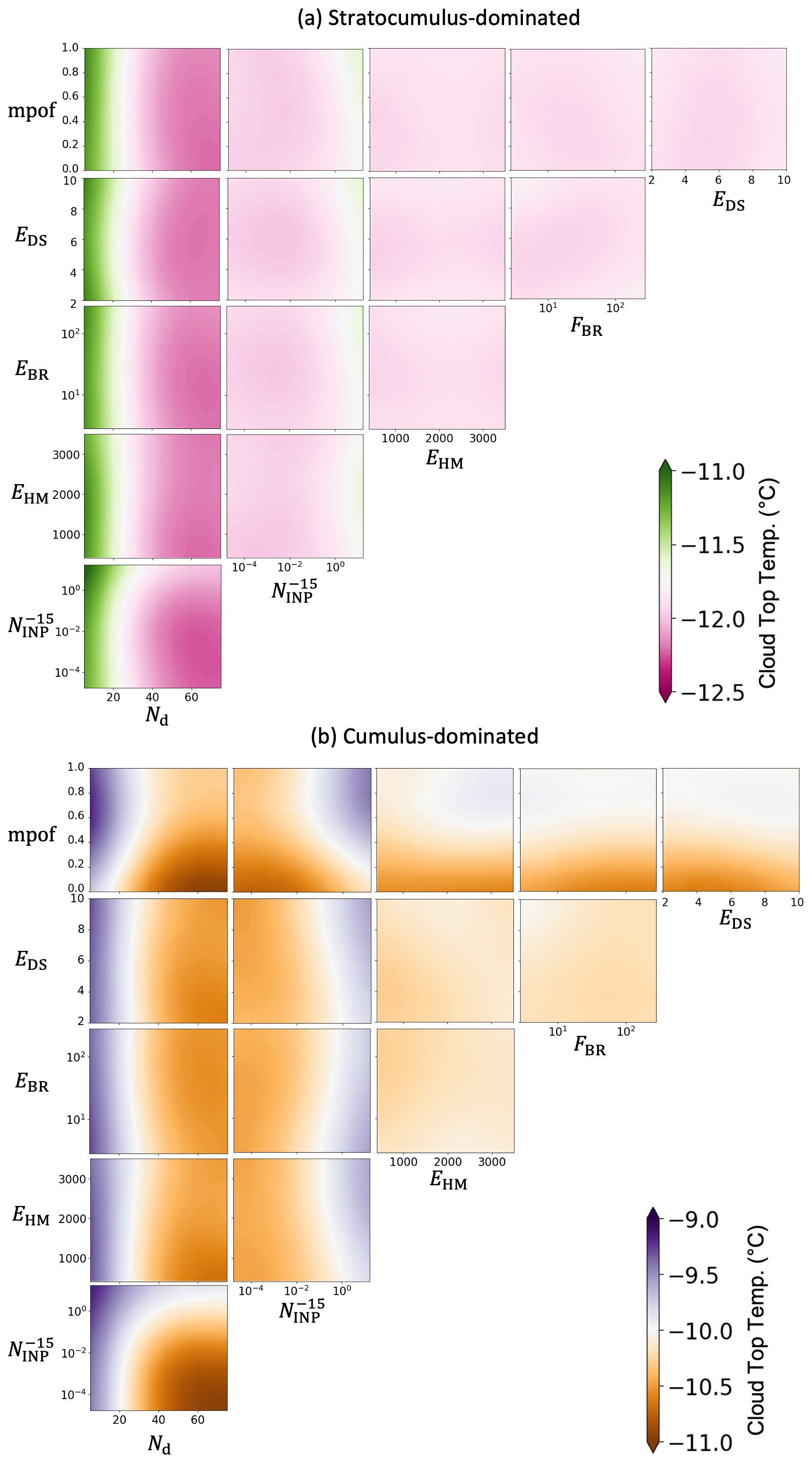
Figure F4 Projected mean model responses of cloud top temperature to paired parameters in (a) Sc region and (b) Cu region.

Appendix G: Results from the global sensitivity analysis

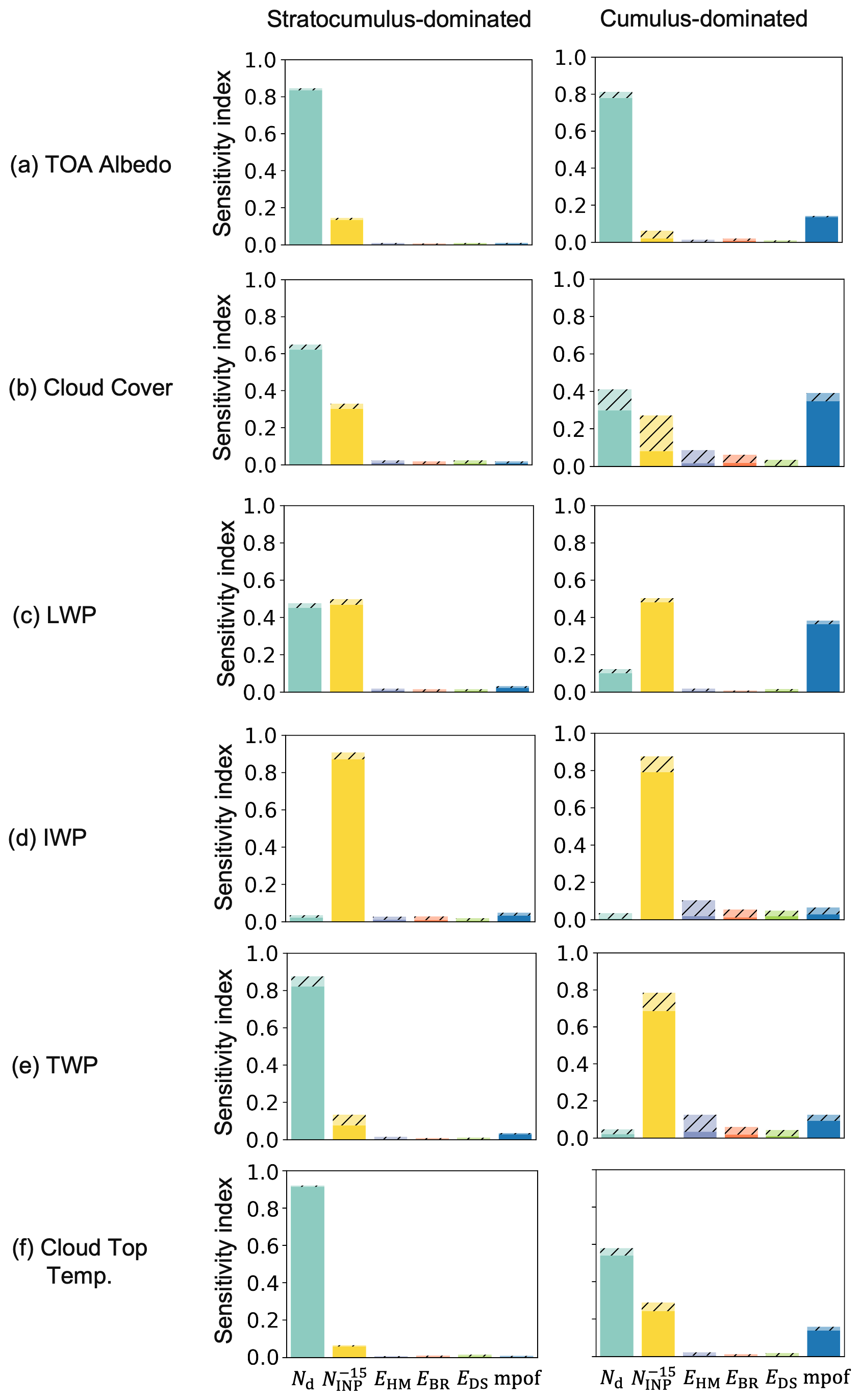
Figure G1 Sensitivity indices of all the perturbed parameters for TOA albedo (unitless), cloud cover (unitless), all-sky LWP (g m⁻²), all-sky IWP (g m⁻²), all-sky TWP (g m⁻²), and cloud top temperature (°C). Each sensitivity index consists of the first-order, main effect (solid fill) and the second-order, interactive effects (dashed). Indices are shown separately for the Sc (left column) and Cu (right column) regions.

A variance-based sensitivity analysis was also performed to quantify the sensitivities of model variables to the perturbed parameters based on a dense sampling of the emulated parameter space (Saltelli et al., 2000). We used the Sobol' method (Saltelli et al., 2000) with the Python library SALib (Usher et al., 2016) to calculate the sensitivity indices. The first-order sensitivity index measures the main effect of each parameter on a model variable. The total sensitivity index includes both the main effect and any additional effects from interactions with other parameters. Therefore, the difference between the total index and the first-order index indicates how much of a parameter's influence comes from its interactions with other parameters (interactive effects) (Johnson et al., 2015).

Figure G1 shows the sensitivity indices over the whole parameter space. This comparison allows us to quantitatively investigate the dominant parameters for the cloud properties in this CAO event over the 6-D parameter space, rather than, as shown in the paired projections, limiting to the values averaged across the parameter space for the non-paired parameters.

In this CAO case, N_d dominates the TOA albedo in both regions and exerts strong influences on cloud cover and LWP. In contrast, IWP in both regions has little sensitivity to the perturbations of N_d. The strong control of N_d over the TOA albedo suggests that an accurate representation of N_d and associated processes, including background aerosol fields, droplet activation of CCN and in-cloud processing of CCN, is essential to accurately represent these mixed-phase clouds in simulations.

$N_{\text{INP}}^{-\mathrm{15}}$ has a strong control of all-sky LWP and IWP in both regions of this CAO case, but its effect on TOA albedo is much weaker compared to N_d. In the Cu region, a high $N_{\text{INP}}^{-\mathrm{15}}$ leads to a reduction in LWP but also an increase in IWP, therefore, its overall influence on TWP is compensated. Although $N_{\text{INP}}^{-\mathrm{15}}$ strongly influences LWP in both cases, its weaker influence on TOA albedo compared to the influence from N_d suggests that, in this CAO case, the Twomey effect associated with perturbations in N_d plays a more dominant role in determining the radiative properties of CAO clouds. As a result, TOA albedo exhibits more sensitivity to perturbations of N_d than to $N_{\text{INP}}^{-\mathrm{15}}$. It is also worth noting here that because the cloud temperature in our case is warm (with a cloud top temperature around −15 °C), the INP concentrations are generally low. Most of the perturbed $N_{\text{INP}}^{-\mathrm{15}}$ is below 1 L⁻¹, which is smaller than the threshold suggested from Vergara-Temprado et al. (2018) for INP to have a strong effect on TOA albedo.

In this CAO case, all SIP parameters (E_HM, E_BR, and E_DS) have generally weak influence on the cloud radiative properties in both regions, compared to other parameters. Comparing the different regions shows that the influence from SIP processes on cloud properties is relatively enhanced in the Cu region, as the clouds deepen and IWP increases with more snow and graupel formations. Most of their influences on cloud cover are interactive effects, suggesting an additional dependency on other parameters. Among the three SIP parameters, E_HM has the strongest influence on LWP, IWP and TWP. This occurs because most cloud temperatures in this case (ranging from −5 to −15 °C) are warmer than the peak temperature for the ice-ice collision (−21 °C) and droplet shattering (−15 °C) processes, but within the temperature range for the HM process (−7.5 to −2.5 °C) which peaks at −5 °C. Therefore, the sensitivities of cloud properties to the parameters shown here are case specific; this point will be further discussed in the Discussion section.

The influences of mpof are weak in the Sc region, but become much stronger in the Cu region for cloud cover and LWP, where IWP increased a lot compared to the ones in the Sc region. Its effects on TOA albedo are also enhanced in the Cu region, but much weaker compared to the those from N_d. The explanation is similar to $N_{\text{INP}}^{-\mathrm{15}}$, as in this case, the radiative properties of CAO clouds are dominated by the Twomey effect associated with perturbations in N_d, rather than the change in LWP. The mpof parameter controls the extent to which liquid and ice hydrometeors interact with each other, and our results suggest that for cloud cover and LWP in the Cu region, it is important to have a good representation of the degree of overlap between ice and liquid hydrometeors. However, mpof remains poorly constrained in models (Abel et al., 2017; Korolev and Milbrandt, 2022; Evans et al., 2025) and can lead to large uncertainties in estimating mixed-phase cloud behaviours under the warming climate and their influences to the Earth's energy budget.