Summertime ozone sensitivity to temperature in China: observational evidence and mechanistic attribution in urban and rural areas in the Yangtze River Delta region

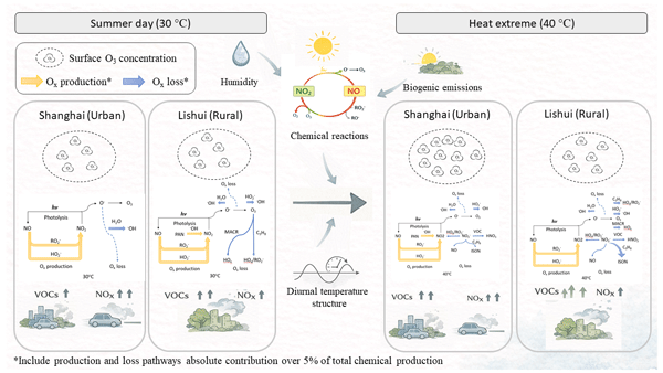
As climate change increases frequency and intensity of hot extremes, understanding how elevated temperatures influence surface ozone (O₃) across different chemical regimes is critical. We combine observations from summer 2022 in the Yangtze River Delta (YRD) with controlled United Kingdom Chemistry and Aerosols (UKCA) Box experiments for urban Shanghai and a lower-NO_x, biogenically influenced Lishui regional environment. Observed daily-maximum O₃ increases with temperature at both sites, with a stronger response in Shanghai. Two-dimensional T-RH distributions show that O₃ rises with temperature and decreases with relative humidity (RH), implying that part of the temperature response is mediated by drying. Factorial box-model experiments separate the roles of temperature-driven shifts in chemical partitioning, diurnal thermal structure, temperature-dependent isoprene emissions, and humidity. In Shanghai, the increase in O₃ between 30 and 40 °C is dominated by BVOC-driven chemistry, with temperature-amplified isoprene emissions explaining most of the observed response. In Lishui, O₃ sensitivity is governed primarily by radical-NO_x chemistry and thermal PAN-NO_x cycling, with a much smaller role for BVOCs. Fixed RH scenarios substantially reduce the apparent contribution of “thermal chemistry”, highlighting humidity-dependent O_x loss and HO_x-NO_x cycling as key modifiers of the climate penalty. Because the 0-D framework excludes transport and meteorological dynamics, the reported fractions isolate the local chemical and emission-driven component of the O₃-temperature relationship. Within this scope, the results identify robust regime-specific mechanisms linking heat, humidity, precursor chemistry, and surface O₃ in the YRD and demonstrate the value of observation-constrained box models as a bridge to regional chemistry-climate simulations.

1 Introduction

Surface ozone (O₃) remains a prominent air-quality and public-health concern, and its variability reflects a tight coupling between meteorology (temperature, humidity, stability, radiation, etc.) and precursor emissions, with co-occurring heat and O₃ extremes documented (Bloomer et al., 2010; Wang et al., 2022a). As heat extremes, e.g., heatwaves (HWs), increase in frequency, duration, and intensity under continued warming (World Meteorological Organization, 2019), quantifying how O₃ responds to hot conditions is becoming increasingly critical for policymakers (Ebi et al., 2021). In China, summertime O₃ has remained elevated despite recent controls on nitrogen oxides (${\mathrm{NO}}_x=\mathrm{NO}+{\mathrm{NO}}_{\mathrm{2}}$), underscoring the need to diagnose the meteorological and chemical drivers of O₃ during hot periods (Wang et al., 2022b).

Ozone is a significant air pollutant that adversely affects human health, particularly respiratory functions. Exposure to elevated O₃ concentrations has been linked to increasing rates of respiratory diseases, including asthma and other pulmonary disorders (Cohen et al., 2017; Pope et al., 2023). The Global Burden of Disease Study (Forouzanfar et al., 2015) estimated that in 2015 alone, approximately 254 000 fatalities were attributed to O₃ exposure worldwide, with about 55 300 to 80 300 of those deaths occurring in China (Cohen et al., 2017; Liu et al., 2018). The impacts extend beyond human health: high O₃ levels impair plant physiological processes, detrimentally affect crop yields, and hinder biomass accumulation, thereby threatening food security and ecosystem stability (Meehl et al., 2018; Meng et al., 2023). Moreover, O₃ is also a significant greenhouse gas that further enhances surface warming (Szopa et al., 2021), with positive feedbacks on O₃ levels (Meng et al., 2023).

The underlying relationship between high temperatures and the resultant increase in surface O₃ concentration can be modulated by four primary mechanisms: (i) emissions of O₃ precursors (NO_x and VOCs), (ii) rates of chemical reaction, (iii) transport and entrainment from the free troposphere, and (iv) deposition of O₃ and its precursors. The meteorological conditions associated with high-temperature events are the key mediators in each pathway and provide the causal links between temperature and the surface O₃ response.

• i.

  Emissions. The production and destruction of O₃ are highly dependent on its precursors, particularly NO_x and volatile organic compounds (VOCs) (Liu et al., 2021b; Solberg et al., 2008). Biogenic VOC (BVOC) emissions, especially isoprene (C₅H₈), increase exponentially with leaf temperature and light intensity, amplifying O₃ formation under warm, sunny conditions (Chen et al., 2022; Ma et al., 2022a). In addition to BVOC emissions, temperature-dependent evaporative anthropogenic VOC (AVOC) sources, such as petrochemical processing, solvents, and vehicles, will also increase with temperature and have a significant impact in urban environments (Wu et al., 2024; Yamada, 2013).

• ii.

  Chemistry. High temperatures impact net photochemical processing in the NO_x-hydrogen oxides (${\mathrm{HO}}_x=\mathrm{OH}+{\mathrm{HO}}_{\mathrm{2}}$)-VOC system by changing rate coefficients, while enhanced actinic flux under persistent clear-sky conditions during heat extremes always increases photolysis rates; the shift in the radical budget generally results in a net production of O₃, although the reaction rates of several important processes are negatively correlated with increasing temperature (Archibald et al., 2020b; Gu et al., 2020). Thermal decomposition of peroxyacyl nitrate (PAN) type reservoirs (e.g., CH₃C(O)OONO₂ (PAN) → CH₃C(O)OO• (PA) + NO₂) at high temperatures further shifts reactive nitrogen toward NO_x, enriching O₃ precursor in local environments (Steiner et al., 2010; Wu et al., 2008). In addition, low humidity at high-temperature conditions reduces the impact of the reaction O(¹D) + H₂O → 2OH, thus favouring net O₃ production (Li et al., 2021).

• iii.

  Transport. High-temperature extremes like HWs frequently coincide with synoptic stagnation, weak circulation and ventilation, and a deeper planetary boundary layer (PBL) (Archibald et al., 2020b; Duc et al., 2022; Utembe et al., 2018; Wu et al., 2019). Stagnation and weak ventilation consistently concentrate O₃ and its precursors, reducing dilution and export, thereby strengthening near-surface accumulation during hot periods (Zhang et al., 2018). On the other hand, a deeper boundary layer at high temperatures generally enhances the ventilation of surface O₃, thereby making it harder for ground-level O₃ to build up (Pfister et al., 2014). The impact of a deeper boundary layer ventilation at high temperatures is partly offset by O₃ entrained from the residual layer aloft (Bloomer et al., 2010).

• iv.

  Deposition. The deposition velocity (V_d) of O₃ and its precursors is often parameterised as $V_{\mathrm{d}}=(R_{\mathrm{a}}+R_{\mathrm{b}}+R_{\mathrm{c}}{)}^{-\mathrm{1}}$, which represents O₃ deposition as a function of an aerodynamic resistance (R_a), a quasi-laminar boundary layer resistance (R_b), and overall canopy resistance (R_c; stomatal + cuticular + soil) (Stella et al., 2011; Zhang et al., 2003). Here, R_a represents turbulent transport above the canopy (mainly affected by wind speed and stability), R_b describes a quasi-laminar boundary layer resistance for vegetation that depends on the diffusion coefficient of species, and R_c is the surface resistance, combining stomatal, cuticular and soil resistances (Clifton et al., 2020b; Wesely, 1989). During high-temperature extremes, synoptic stagnation and weak near-surface winds reduce turbulent transport near the surface, increasing R_a and R_b resistances and thereby lowering deposition velocity (Wesely, 1989; Zhang et al., 2003). Under hot and dry conditions, high vapour pressure deficit (VPD) and depleted soil moisture reduce stomatal conductance, so the stomatal part of R_c increases, lowering V_d for stomata-controlled species (O₃, NO₂) (Kavassalis and Murphy, 2017; Wilson et al., 2022). Concurrently, hot/dry leaves have minimal surface water films, which raises cuticular resistance and further increases R_c (Clifton et al., 2020b). In contrast, dry soils tend to exhibit lower soil resistance than moist soils, so soil/litter uptake of O₃ strengthens as surfaces dry – partly offsetting the stomatal signal. (Clifton et al., 2020a; Stella et al., 2011).

Complicating this picture are spatial variations in precursor-sensitivity regimes. In NO_x-limited (VOC-rich) environments – typically found in rural and regions downwind of ozone precursor emissions – O₃ production increases nearly linearly with NO_x concentrations and shows limited sensitivity to further VOC additions (Steiner et al., 2006; Utembe et al., 2018). Conversely, in highly urbanised areas with high ${\mathrm{NO}}_x/\mathrm{VOC}$ ratios (VOC-limited regime), additional NO_x (mainly emitted in the form of NO) can suppress O₃ by titrating ozone back to NO₂ (${\mathrm{O}}_{\mathrm{3}}+\mathrm{NO}\to {\mathrm{NO}}_{\mathrm{2}}+{\mathrm{O}}_{\mathrm{2}}$), and O₃ formation becomes more strongly driven by available VOCs (Simon et al., 2015). The existence of two regimes implies that identical temperature-driven chemical and meteorological forcings can yield contrasting O₃ responses if background pollutant levels differ, such as in urban versus rural settings, highlighting the need to assess urban-rural differences explicitly.

Most observation-based studies indicated a positive correlation between temperature and tropospheric O₃ levels as a result of the combined effects of O₃'s temperature responses, while some reported a non-monotonic relationship between temperature and climate penalty factor (O₃-temperature slope, $\mathrm{\Delta }{\mathrm{O}}_{\mathrm{3}}/\mathrm{\Delta }T$) when ambient temperature exceeds thresholds (Kalisa et al., 2018; Nguyen et al., 2022; Ning et al., 2022; Pusede et al., 2015; Shen et al., 2016; Steiner et al., 2010). Unravelling this complexity requires a careful distinction of how temperature interacts with various atmospheric factors, including solar radiation, humidity, planetary boundary layer height (PBLH), wind speed, precipitation, and both anthropogenic and biogenic emissions (Bloomer et al., 2010; Nguyen et al., 2022; Sun et al., 2017; Wang et al., 2022a; Wu et al., 2008).

Despite the growing body of work on O₃-temperature coupling, significant gaps remain. Observation-constrained box models treat each site as a well-mixed air parcel, apply detailed chemical mechanisms to diagnose local photochemical production and loss rates, provide adjustable environmental parameters, and help separate local chemical controls from transport influences, and are therefore a useful complement to 3-D chemical transport models in studies of extremes (McDuffie et al., 2016). However, few studies have combined observations with process-level box-model budget analyses to quantify the relative contributions of chemical kinetics and precursor changes under extreme-heat conditions. Besides, urban-rural contrasts in O₃ temperature sensitivity have not been systematically explored using consistent methodological frameworks. This is particularly true for rapidly urbanising regions of East Asia, where emission patterns and warming trends interact to shape local O₃ dynamics.

In this study, we investigate the mechanisms of surface O₃'s chemical response to high temperatures in two contrasting environments within the Yangtze River Delta (YRD) in China: urban Shanghai and rural (forest-influenced) Lishui. Focusing on summer 2022, we combine surface observations with controlled UKCA Box experiments over a temperature range of 25–40 °C. The box-model experiments isolate temperature-dependent gas-phase chemistry, humidity effects, diurnal thermal structure, and temperature-dependent isoprene emissions, allowing the O₃ response to be attributed to local chemical and emission-related processes under prescribed environmental conditions. By quantifying O₃ production, chemical loss, and deposition of ozone and precursors, we then identify how the two chemical regimes respond differently to warming.

The attribution presented in this study focused on processes that can be isolated within the UKCA Box model. Within this framework, we isolate the local chemical and precursor-emission responses to temperature with prescribed environmental conditions. Consequently, three-dimensional physical influences such as transport, entrainment, boundary-layer development, stagnation, clouds, and precipitation are not separately resolved. Our attribution therefore addresses the chemical component of the O₃-temperature relationship.

2 Data and Methods

2.1 Study Locations and Observations

The locations of the monitoring sites, the YRD urban boundaries, and the NO₂ gradient are shown in Fig. 1.

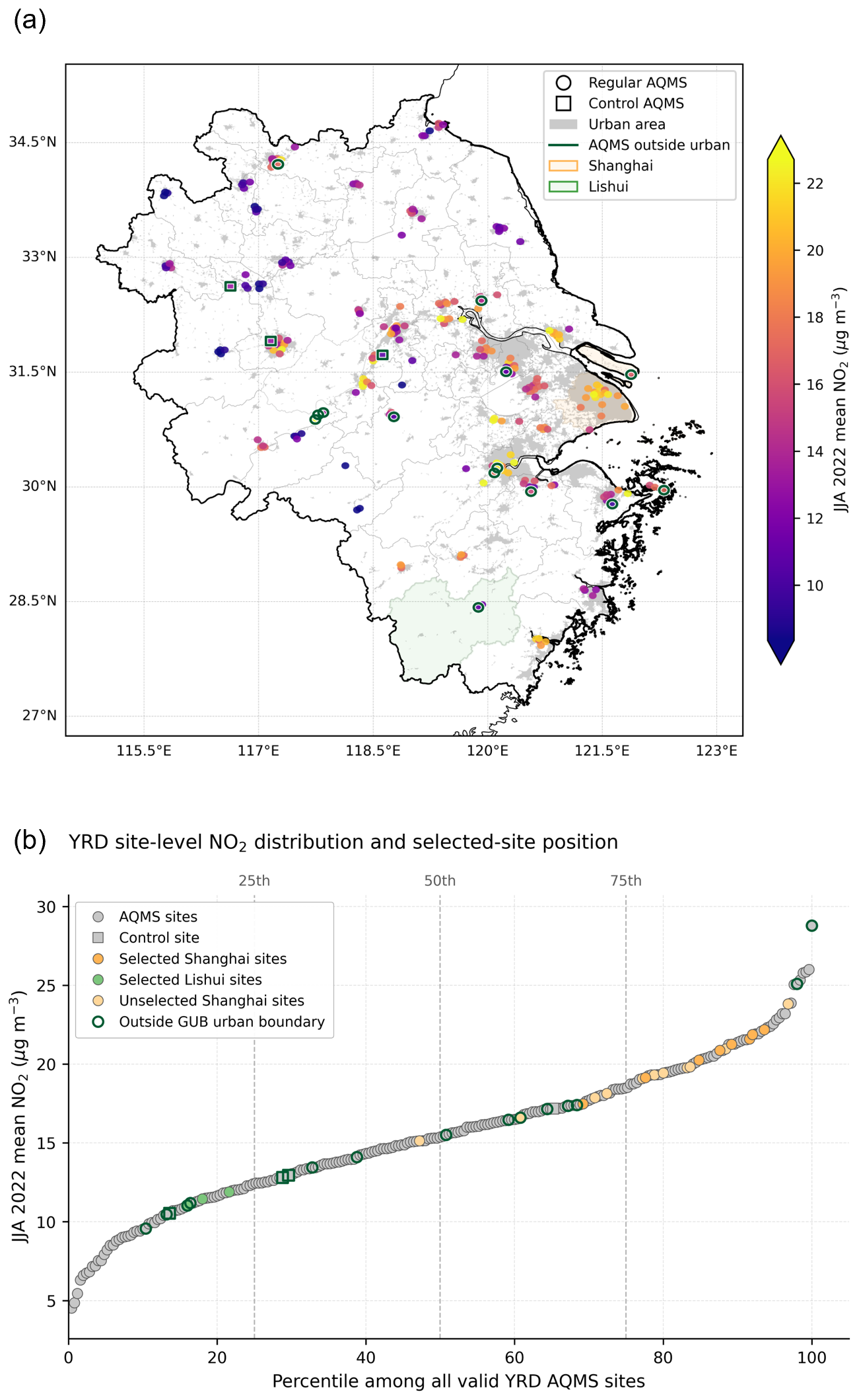
Figure 1 (a) Spatial distribution of Air Quality Monitoring Sites (AQMS) across the YRD in summer 2022, coloured by JJA 2022 mean NO₂. Grey shading indicates the 2018 Global Urban Boundaries (GUB) urban settlement extent. Circular markers denote regular AQMS, square markers denote control sites, and green outlines indicate sites located outside the GUB urban settlement boundary. Shanghai and Lishui are highlighted by coloured city polygons. (b) Ranked distribution of JJA 2022 mean NO₂ across all valid YRD AQMS, expressed as site percentile. Selected Shanghai and Lishui sites (listed in Table 1) are highlighted in orange and green, respectively; unselected Shanghai sites are shown in pale orange, and sites outside the GUB urban boundary are outlined in dark green. Administrative boundaries from the GADM database (http://www.gadm.org, last access: 11 March 2026).

The observational analysis uses surface air-quality measurements from Shanghai and Lishui as two contrasting environments within the YRD. Shanghai represents a densely urbanised megacity environment with strong anthropogenic precursor influence, while Lishui provides a lower-NO_x environment with stronger influence from surrounding vegetated areas. These two cases are used to examine how O₃-temperature sensitivity differs across contrasting precursor and land-surface settings.

To place the selected monitoring sites within the broader YRD context, AQMS locations were compared with the 2018 Global Urban Boundary (GUB) dataset (Li et al., 2020). The GUB dataset delineates physical urban extents at 30 m resolution using Global Artificial Impervious Area (GAIA) data. The 2018 boundaries were used to identify whether individual AQMS sites were located within or outside mapped urban areas.

The YRD-wide comparison included 250 valid AQMS sites in JJA 2022. Validation defined by hourly data in June–August (JJA) 2022 with a threshold of 75 %. The selected Shanghai sites are located within GUB urban settlement polygons and occupy the high-NO₂ part of the YRD AQMS distribution, with a mean NO₂ concentration of 20.58 µg m⁻³, corresponding to approximately the 87th percentile among valid YRD sites.

The selected Lishui sites occupy a lower-NO₂ part of the YRD AQMS distribution, with a mean NO₂ concentration of 11.46 µg m⁻³, corresponding to approximately the 18th percentile among valid YRD sites. Two of the three selected Lishui sites fall within GUB urban settlement polygons, indicating populated urban/suburban receptor locations within a broader lower-NO_x and more biogenically influenced regional setting.

As far as population density and land-use type are concerned, Shanghai is a megacity with a population density of 3900 km⁻² (Shanghai Municipal Statistics Bureau, 2024), and construction land covered 42.4 % of its total area (Gong et al., 2022). Lishui is an area where 81.7 % of the land is covered with forest (Tang et al., 2022). The population density of Lishui is 140 km⁻², and the urban district accounts for about 8.6 % of its total area (Lishui Municipal Statistics Bureau, 2025).

We collected ground-level hourly O₃ observation data from the China National Environmental Monitoring Center (CNEMC). The AQMS are in the busiest areas of Shanghai (30.67–31.88° N, 120.85–122.2° E) and in the populated centre area of Lishui (27.44–28.78° N, 118.70–120.41° E).

The analysis focuses on JJA 2022, when the YRD experienced severe and persistent high-temperature conditions. This period provides a well-observed recent heatwave case with routine surface O₃ measurements from the national monitoring network. Earlier major heatwave summers in the region, such as 2003 and 2013, predate the availability of constant O₃ observations (see https://quotsoft.net/air/, last access: 14 July 2025). The 2022 data are therefore used to examine O₃-temperature sensitivity under a heat extreme setting.

We assessed O₃ and meteorological data for June–August 2022 (JJA 2022). Eight AQMS and two Meteorological Monitoring Sites (MMS) in Shanghai, and three AQMSs and one MMS in Lishui met this criterion (spatial distribution see Fig. 1). For each retained site, we extracted hourly surface O₃ and then formed two aggregated series: an urban mean (average across the 8 Shanghai sites at each hour) and a rural mean (average across the 3 Lishui sites at each hour). Meteorological observations originate from the China Meteorological Monitoring System (CMMS) stations; we accessed the archived data via the NOAA National Climatic Data Center (NCDC).

The meteorological and air-quality monitoring sites retained for the analysis are summarised in Table 1 below.

Table 1 Information on the MMS (XJH, BS, and LS) and AQMS in SH and LS.

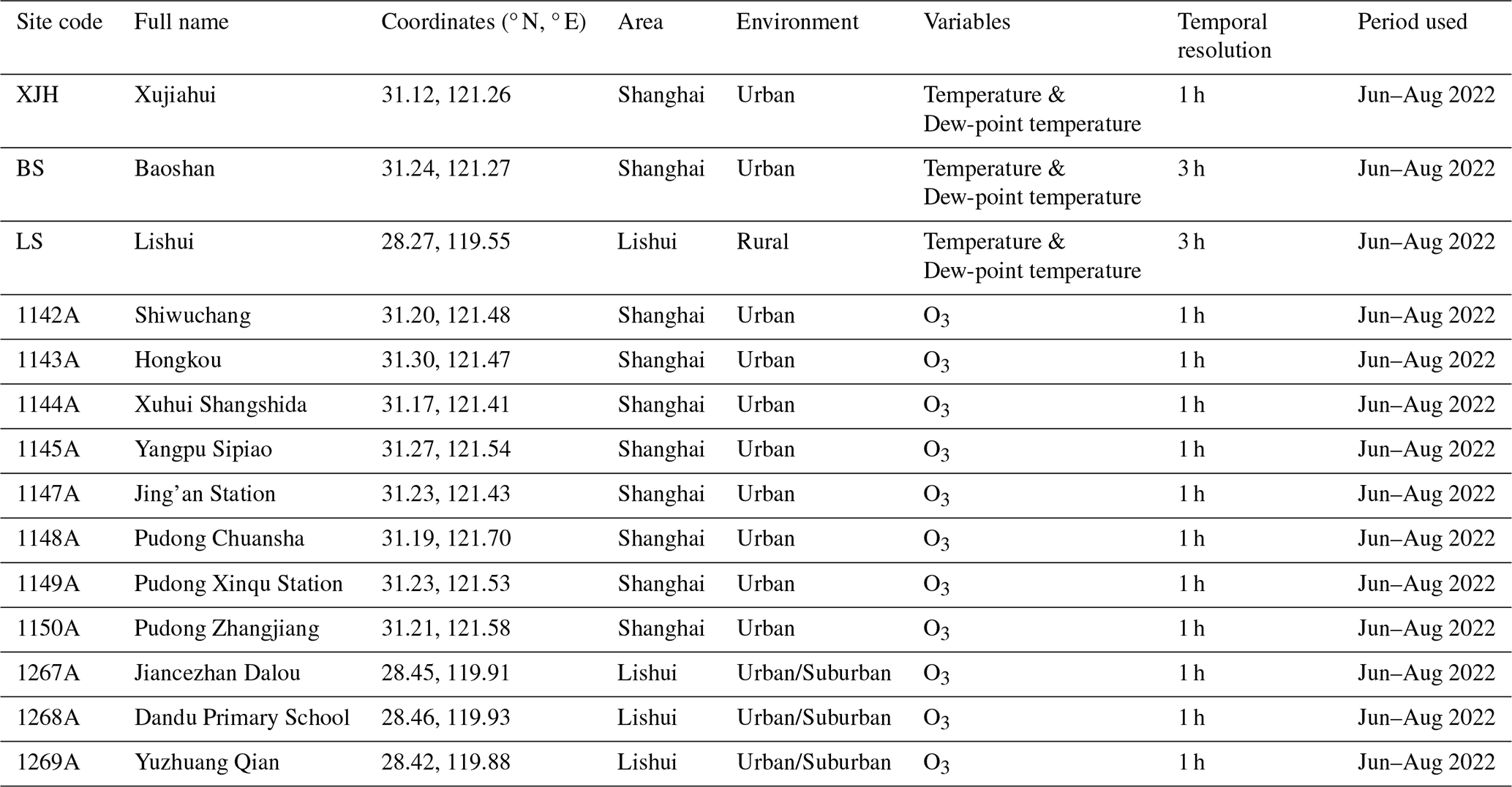
The AQMSs in Lishui (1267A–1269A; Table 1) are located in a populated environment that is best characterised as urban or suburban. The Lishui emission inputs used in the box model (explained later in Sect. 2.2), however, represent regional mean conditions with relatively low NO_x and stronger biogenic influence. The resulting chemical regime therefore characterises the regional photochemical environment influencing Lishui, rather than the immediate atmosphere at the monitoring sites.

In this study, a heatwave is defined as a period of at least 3 consecutive days during which the daily maximum temperature exceeds the 90th percentile of the reference period (2000–2019), as used by Zhao et al. (2019). The 90th percentile threshold has been widely used in studies examining heatwave patterns, health impacts, and interactions with air quality (Engdaw et al., 2022; Fischer and Schär, 2010; Sun et al., 2020). To remove day-to-day variation, a 15 d smoothing window centred on the investigated day was applied to threshold calculation (based on the reference period) (García-Martínez and Bollasina, 2021). The years 2020 and 2021 were excluded from the reference period calculation to eliminate any effects resulting from the COVID-19 lockdowns in China.

For the ozone-temperature analysis, we use daily maximum surface O₃ (O_3max) and daily maximum air temperature (T_max) because climate-penalty assessments are conventionally based on daily peak metrics (e.g. daily max 1 h O₃ versus daily T_max), which target the photochemical period, reduce confounding nocturnal NO-titration and inter-site timing offsets (Nolte et al., 2021; Otero et al., 2021). We stratify by environment type (urban Shanghai vs. rural Lishui) and by period (all JJA days vs. heatwave days), thus yielding four subsets of ozone-temperature analysis: urban-all, urban-HW, rural-all, and rural-HW.

The XJH site (Shanghai; 31.12° N, 121.26° E) reports hourly air temperature and dew-point temperature. The BS site (Shanghai; 31.24° N, 121.27° E) and the LS site (Lishui; 28.27° N, 119.55° E) provide three-hourly records of air temperature and dew-point temperature. Daily maximum air temperature values at sites XJH and BS were averaged to obtain the representative Shanghai temperature conditions. To evaluate the joint influence of surface air temperature and humidity on ground-level O₃, we aligned the temporal resolution by applying a 3 h mean to the hourly O₃ series, ensuring that O₃, temperature, and humidity share the same 3-hourly meteorological sampling times.

2.2 Model configurations and inputs

2.2.1 UKCA Box model configuration

We use the United Kingdom Chemistry and Aerosols (UKCA) Box Model (equivalent to the Unified Model (UM) version 13.0), which executes the identical UKCA chemistry-aerosol code used in the Met Office UM over a single grid cell (1.25° × 1.9°; zero-D), run independently of the UM. The UKCA Box Model, like other box models, treats each site as a well-mixed air parcel, provides adjustable environmental parameters, and helps separate the contributions of local chemical controls (McDuffie et al., 2016). The box model, by design, does not include advection, convection, and diffusion, enabling fast simulations with direct code-level traceability to UM-UKCA/UK Earth System Model (UKESM) (UKCA, 2025).

Compared to the full 3-D UM-UKCA (e.g. UKESM-AMIP), the box model isolates local chemical-microphysical responses to prescribed forcings (temperature, humidity, photolysis) without transport processes, and completes controlled perturbation experiments orders of magnitude faster, while retaining the StratTrop chemical mechanism used in UKESM1 (Archibald et al., 2020a; UKCA, 2025).

The aim of the UKCA Box model simulation in this study is to build two contrasting chemical environments: an urban case dominated by anthropogenic transport/industrial emissions (Shanghai-like chemical environment) and a rural case dominated by biogenic VOC emissions (Lishui-like chemical environment). The highly controllable climate forcing enables attribution of the O₃ temperature response to (1) chemical-kinetic temperature dependence, (2) the dependence of the chemistry on humidity, (3) temperature dependence of BVOC (isoprene) emissions, and (4) diurnal temperature structure. A 3-D UKESM-AMIP simulation was performed to compare the box against a fully resolved chemistry-meteorology system, providing grid-cell-mean O₃ production and loss diagnostics under the same chemistry scheme and indicating the budget contributions absent from the box configuration, particularly transport/export. To ensure comparability and avoid ambiguity arising from administrative-area differences between Shanghai and Lishui, O₃ budget calculations were carried out by configuring the box to match the UM grid size (1.25° × 1.9°). The emission and deposition inputs used to define these baseline environments are described below with Fig. 2 and Supplement.

In the box model simulations in this study, photolysis varies diurnally with the solar-zenith angle at the target latitude/longitude. Prescribed meteorological inputs were held at the baseline values (70 % RH when at 30 °C, Pressure = 1000 hPa, and PBLH = 590 m), which are consistent with YRD summer-average values. The temperature and humidity perturbation settings are described in Table 3 (see Sect. 2.3).

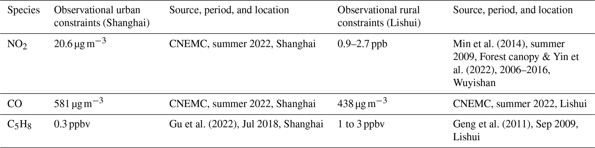
We repeat a representative summer-day radiation cycle until the system attains a steady state (defined as a state in which the variation in the output daily mean values of key chemical species is within ±0.1 % of the previous day). To avoid analysing relatively unimportant partitioning between O₃ and closely related odd-oxygen species, we focus our analysis on the wider odd-oxygen family (O_x) (using UKCA definition as ${\mathrm{O}}_x={\mathrm{O}}_{\mathrm{3}}+\mathrm{O}{(}^{\mathrm{1}}\mathrm{D})+\mathrm{O}{(}^{\mathrm{3}}\mathrm{P})+{\mathrm{NO}}_{\mathrm{2}}+\mathrm{2}{\mathrm{NO}}_{\mathrm{3}}+\mathrm{3}{\mathrm{N}}_{\mathrm{2}}{\mathrm{O}}_{\mathrm{5}}+{\mathrm{HNO}}_{\mathrm{4}}+{\mathrm{HNO}}_{\mathrm{3}}+\text{PANs}$) (Bates and Jacob, 2020; Hu et al., 2017). The model time resolution is 10 min. Initial trace-gas fields follow the standard ST_urban UKCA box initial-condition set, except the initial concentrations of key O₃ precursors, the concentrations of which are consistent with observations where available (See NO₂, CO, and C₅H₈ in Table 2; see other observations in Table S1 in the Supplement). Localised adjustments to emissions, deposition, and selected baseline species are described below and in Tables S1 and S3.

Table 2 Observational NO₂, CO, and C₅H₈ constraints for key species used to define the Shanghai- and Lishui-like baseline chemical environments.

To show how the inventory fields were translated into the two box-model environments, Fig. 2 presents the spatial selection of CEDS emissions together with the final anthropogenic and biogenic emission inputs used for Shanghai and Lishui.

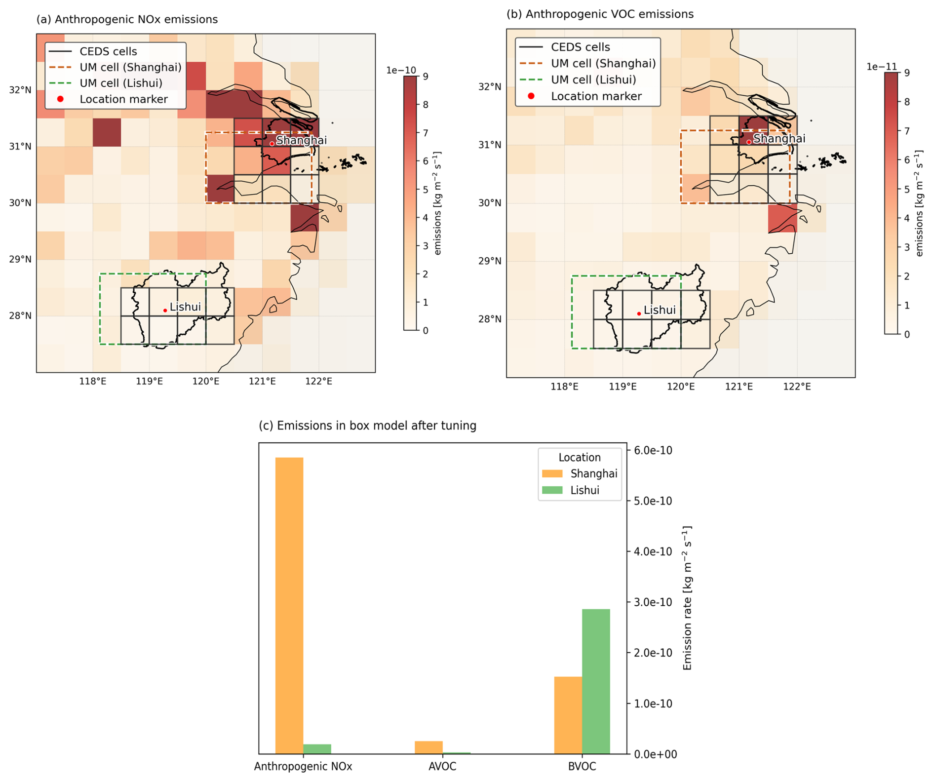
Figure 2 Anthropogenic and biogenic emission fields and box-model emission inputs. (a) CEDS anthropogenic NO_x emissions over the study region for JJA 2022 (kg NO m⁻² s⁻¹). (b) CEDS anthropogenic VOC species included in the box-model emission input, calculated as the sum of C₂H₆, C₃H₈, and HCHO emissions (kg VOC m⁻² s⁻¹). (a, b) Spatial selection used to define the Shanghai and Lishui model emissions: municipal outlines (black); Grey cells indicate the CEDS grid cells selected to calculate the Shanghai and Lishui anthropogenic emission inputs. The dashed orange (Shanghai) and green (Lishui) outlines show the corresponding grid cells used in the UKESM-AMIP and are included only to show their spatial relationship to the selected CEDS cells. (c) Final box-model emission inputs for anthropogenic NO_x, sum of AVOC species included in the box-model input, and BVOCs (units: $\mathrm{kg}{\mathrm{m}}^{-\mathrm{2}}{\mathrm{s}}^{-\mathrm{1}}$). Coastlines from Natural Earth (naturalearthdata.com). Administrative boundaries from the GADM database (http://www.gadm.org, last access: 11 March 2026).

Anthropogenic emissions were prescribed from the Community Emissions Data System (CEDS; version 2024_11_25) for JJA 2022. The dashed UKCA/UM grid-cell outlines in Fig. 2 are shown only to indicate the spatial relationship between the box-model emission selection and the UKESM-AMIP grid cells; they were not used to calculate or average the CEDS emission inputs. The anthropogenic VOC input included the emitted tracers available in the StratTrop box configuration, C₂H₆, C₃H₈, and HCHO, and therefore represents an effective subset rather than the complete urban AVOC mixture. Biogenic emissions of C₅H₈ and monoterpenes (Monoterp) were based on the MEGAN v2.1 inventory for China reported by Wu et al. (2020). Dry deposition was applied using the UKCA implementation of the Wesely (1989) resistance scheme for O₃, CO, HCHO, NO₂, and the deposited NO_y species (include NO, NO₂, NO₃, N₂O₅, HO₂NO₂, HNO₂, PAN, PPAN, and MPAN) represented in the mechanism. Table 2 summarises the principal observational constraints used to establish the two baseline environments.

The inventory-derived emissions and standard deposition terms were used as the starting inputs, but they could not be applied directly in the closed 0-D system. The absence of horizontal transport, resolved vertical mixing, ventilation, physical export, clouds, and wet removal caused some species to accumulate and others to be removed too rapidly during the repeated clear-sky integrations. Emission and deposition adjustments were therefore treated as effective residual source or loss terms representing these unresolved processes. The objective was to reproduce the available reference concentrations within ±20 % or the observed order of magnitude, prevent unrealistic build-up or over-removal, and retain the intended precursor regime at each site. O₃ was not tuned directly, and its deposition was not adjusted to force agreement with observed O₃.

The remaining constraints were applied according to the chemical role of each species. CO was constrained to within ±20 % of the available observations. Where suitable observations were unavailable, C₂H₆ and C₃H₈ emissions were adjusted only to prevent persistent accumulation or excessive removal. HCHO was used as an integrated indicator of the carbonyl and VOC-oxidation environment instead of being tuned; agreement within ±20 % of observations shows that the model reproduces the overall reactive VOC environment well and supports the adopted effective AVOC representation. O₃, PAN, and other observed species that were not direct constraints were used to evaluate the resulting chemical environment.

For Shanghai, the adjustment was designed to establish a stable high-NO_x, VOC-limited environment. NO₂ deposition was increased to represent unresolved NO_x removal by ventilation and dilution, while the NO emission source was reduced only because inventory-derived NO accumulated in the closed box. Together, these changes maintained NO under stable conditions (defined as daily mean variation of species' concentration within 0.1 %) and reproduced the observed NO₂ level within ±20 %. C₅H₈ and monoterpene emissions were increased to represent the regional biogenic influence of forests south and southwest of Shanghai (Liu and Miao, 2026; Xu et al., 2021). Because the additional C₅H₈ source represents transported regional influence rather than purely local emission, its temperature-dependent component was reduced by 50 % to account conservatively for dilution and chemical loss during transport. The resulting C₅H₈ and monoterpene concentrations remained within the observed order of magnitude.

For Lishui, the adjustment was designed to establish a clean, low-NO_x, NO_x-limited regional environment with strong biogenic influence. The available Lishui air-quality monitoring sites are located in populated urban or suburban areas and were therefore not used as direct NO₂ targets for the regional box environment. Instead, forest-canopy and mountain-background observations provided order-of-magnitude references for NO₂ (see Table 2). The original NO₂ deposition was retained, and the NO source was reduced only when NO accumulated. C₅H₈ emissions were reduced to represent export and dilution from the vegetation-rich source region, producing a daytime C₅H₈ concentration within ±20 % of the available Lishui observation. Monoterpene emissions were retained at their inventory value because suitable observations were unavailable.

The final Shanghai and Lishui emission and deposition settings were fixed before the temperature, humidity, diurnal-cycle, and isoprene-temperature sensitivity experiments. Consequently, the simulated O₃ responses arise from controlled perturbations applied to the same baseline chemical environment rather than from retuning at each temperature. The final scaling factors, observational references, and achieved baseline concentrations are reported in Tables S1–S4. The 2022 observations and inventories define the baseline environments, while the subsequent experiments impose temperatures from 25 to 40 °C under controlled conditions and do not attempt to reproduce the full meteorological evolution of summer 2022.

2.2.2 UKESM-AMIP configuration

A full 3-D UKCA model simulation reproducing the 2022 summer was conducted and compared with the Box model simulations. This simulation was performed using the UKESM-AMIP setup with the UM version 13.3. The model was run with a horizontal resolution of 1.25° by 1.9° (as shown on Fig. 2) with 85 vertical levels up to 85 km (Walters et al., 2019), and the GLOMAP-mode aerosol scheme, which simulates sulfate, sea salt, BC, organic matter, and dust but does not simulate nitrate aerosol (Mulcahy et al., 2020). The chemistry scheme used was Strat-Trop (Archibald et al., 2020a), identical to the box model. Anthropogenic and biomass burning emissions were from the SSP3-7.0 scenario from the CEDS (shown in Fig. 2), as described by Hoesly et al. (2018). Oceanic emissions were from the POET 1990 data set (Olivier et al., 2003), and all biogenic emissions except isoprene and monoterpenes were based on 2001–2010 climatologies from the Model of Emissions of Gases and Aerosols from Nature under the Monitoring Atmospheric Composition and Climate project (MEGAN-MACC) version 2.1 (Guenther et al., 2012). Isoprene and monoterpene emissions were generated interactively using the iBVOC parameterisation and were shown in Fig. 2c (Pacifico et al., 2011).

Temperature and horizontal wind fields were nudged (Telford et al., 2013) in the model run to the ECMWF ERA5 reanalyses for 2022 from ECMWF (Dee et al., 2011) to constrain the atmospheric conditions as close to the observations as possible. Nudging only occurred above ∼1200 m in altitude to avoid surface effects, and thus, the majority of the planetary boundary layer was not nudged.

A 6-month run from 1 March 2022, to 31 August 2022, was conducted with the nudged UKESM-AMIP model. In the UKESM-AMIP input environment settings, monthly sea surface temperature (SST) and sea ice concentration (SIC) under the SSP2-4.5 scenario were used. The first three months are considered the model spin-up. The output of the nudged UKESM-AMIP simulation was provided as monthly mean values, while the grid cells for Shanghai and Lishui were chosen as in Fig. 2.

2.3 Sensitivity experiments

To separate the effects of temperature, humidity, diurnal temperature variation, and temperature-dependent isoprene emissions, we defined 16 sensitivity configurations, summarised in Table 3.

Table 3 Sensitivity experiments of the UKCA Box Model (VRH = fixed absolute humidity (= RH 70 % at 30 °C); FRH = variable absolute humidity (= RH 70 %)).

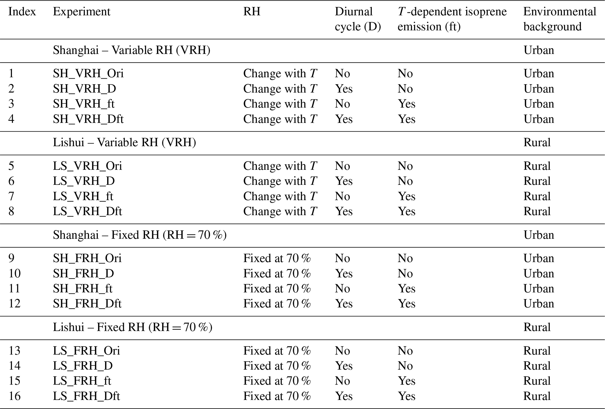
Each of the 16 configurations was repeated at seven target temperatures from 25 to 40 °C at 2.5 °C increments, while all other settings were held according to the experiment definition. These follow the naming convention <location>_<RH>_<process>:

• Location. SH = Shanghai, urban background; LS = Lishui, rural background.

• RH setting. VRH = relative humidity varying with temperature, fixed absolute humidity (= RH 70 % at 30 °C); FRH = relative humidity fixed at 70 %, variable absolute humidity (see Table S2).

• Process. D = diurnal cycle in air temperature enabled; ft = temperature-dependent isoprene emission factor ft enabled; Dft = both enabled; Ori = both disabled

The temperature-dependent isoprene-emission response and the two humidity configurations used in the sensitivity experiments are illustrated in Fig. 3.

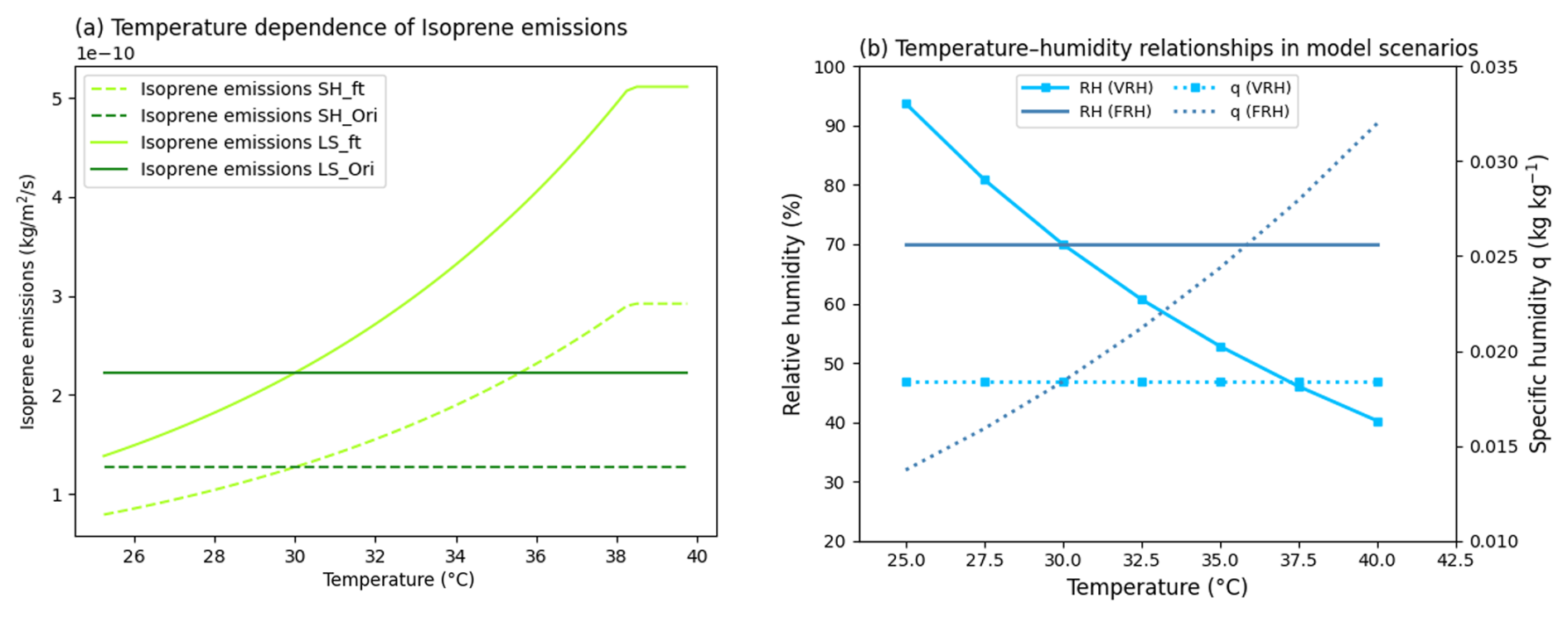
Figure 3 Model settings for the isoprene temperature dependence and the humidity scenarios. (a) Isoprene emission response to temperature used in the sensitivity configurations. Solid lines (LS) and dashed lines (SH) show cases with the temperature-dependent factor ft enabled (_ft) versus the baseline with ft disabled (_Ori, isoprene emissions constant with baseline conditions). The ft response increases with T and saturates at 38.3 °C; emission rates are shown in kg m⁻² d⁻¹ (left axis). (b) Two humidity scenarios respond to temperatures in humidity settings. The VRH case (lines with markers) applies temperature-dependent RH and constant q, while the FRH case (lines) holds constant RH and temperature-dependent q. Axes show RH (%) on the left and q (kg kg⁻¹) on the right.

Two binary switches modify the model processes: D and ft. D (diurnal temperature enabled) applies a realistic diurnal cycle to the target-temperature (daily maximum) day; when D is off, air temperature is held constant at the target value, an extreme condition in which daily minimum values equal daily maximum values. The temperature-dependent isoprene emission factor ft enables the temperature response of isoprene.

The temperature response of isoprene followed the equations below:

$$\begin{array}{}\text{(1)}& \mathrm{\text{isoprene emissions}}=\text{local summer average emissions}\cdot \text{ft}\end{array}$$

The ft is the isoprene temperature dependence factor (Pacifico et al., 2011):

$$\begin{array}{ll}\text{ft}=e^{\mathrm{0.1}\cdot \left(T-\mathrm{30}\right)}& \text{when }{e}^{\mathrm{0.1}\cdot \left(T-\mathrm{30}\right)}<\mathrm{2.3}\left(T\text{ in }\mathrm{°}\mathrm{C}\right)\\ \text{ft}=\mathrm{2.3}& \text{when }{e}^{\mathrm{0.1}\cdot \left(T-\mathrm{30}\right)}\ge \mathrm{2.3}\left(T\text{ in }\mathrm{°}\mathrm{C}\right)\end{array}$$

Where T is temperature in centigrade.

In these experiments, isoprene emissions increase with temperature until they reach their plateau at 38.3 °C (as shown in Fig. 3); when ft is off, isoprene emissions are temperature-independent.

The reference conditions were set at 30 °C and 70 % RH (mass mixing ratio of water (q) = 0.0184 kg kg⁻¹), representing the average environmental conditions in the 2022 JJA summer in the YRD based on observed values. Unless stated otherwise, pressure and boundary-layer height are held at the baseline values (Pressure = 1000 hPa, PBLH = 590 m), which are the averaged YRD summer conditions based on observations and ECMWF ERA5 reanalyses in 2022. Photolysis varies diurnally with the solar zenith angle at the site's latitude/longitude, so it shows a sinusoidal variation peaking at midday and being zero at night. The clouds were ignored, and all simulations are under clear-sky conditions. The location settings determine initial species levels.

The aim of UKCA Box sensitivity experiments is to quantify the local chemical and emission-related response to prescribed temperature and humidity conditions. The results should be interpreted as contributions within this controlled chemical framework, rather than as a full decomposition of all meteorological controls on the observed O₃-temperature relationship.

3 Results

3.1 Observed O₃ response to temperature and humidity variations

The observed relationships between daily maximum O₃ and daily maximum temperature in Shanghai and Lishui are shown in Fig. 4.

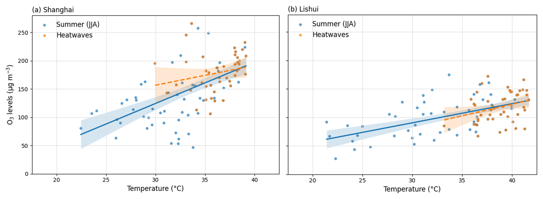
Figure 4 Relationship between observed daily maximum surface ozone concentration and air temperature (based on hourly data) during the summer of 2022 (JJA; blue) and heatwave days (orange; definition see Sect. 2.1) for (a) Shanghai and (b) Lishui. Points are the daily maximum values (average values for sites; spatial distribution shown in Fig. 1); solid (JJA) and dashed (heatwave) lines are ordinary-least-squares fits. Shaded envelopes show the 95 % confidence intervals for the fitted lines.

Across both data subsets (JJA and HW days), and at both locations (Shanghai and Lishui), O_3max increases with T_max, resulting in positive correlations. Averaged over eight Shanghai sites, the summertime O₃ fractional change per unit temperature change is 7.27 $\mathrm{\mu }\mathrm{g}{\mathrm{m}}^{-\mathrm{3}}\mathrm{°}{\mathrm{C}}^{-\mathrm{1}}$ with a 95 % confidence interval (CI) [5.13, 9.41] and p<0.01. The corresponding mean sensitivity across three Lishui sites is 3.36 $\mathrm{\mu }\mathrm{g}{\mathrm{m}}^{-\mathrm{3}}\mathrm{°}{\mathrm{C}}^{-\mathrm{1}}$ (95 % CI [2.30, 4.41], p<0.01).

This urban-rural contrast is consistent with differences in the chemical regime. As reported by Gu et al. (2020), Shanghai exhibits a strong VOC-limited regime in O₃ formation, where temperature increases enhance BVOC emissions while NO_x remains abundant, leading to a relatively strong ozone-temperature relationship. By contrast, the rural areas in YRD generally show higher VOC abundance, and the effect of temperature is less pronounced than in VOC-limited areas because BVOC changes here have a negligible impact (Jin and Holloway, 2015). Those differences in chemical regimes are also supported by model simulation results in this study (Sect. 3.2; Fig. 6). Thus, the doubled O₃ sensitivity to temperature in Shanghai compared to Lishui is consistent with stronger NO_x availability and generally higher pollution levels in Shanghai, and may relate to the capacity for PAN thermal decomposition in the YRD (detailed PAN analysis see Fig. 10) (Steiner et al., 2010).

Regressions during HWs indicate a different behaviour at the two locations. In Lishui, the heatwave-period O_3max–T_max sensitivity is 4.05 $\mathrm{\mu }\mathrm{g}{\mathrm{m}}^{-\mathrm{3}}\mathrm{°}{\mathrm{C}}^{-\mathrm{1}}$ (95 % CI [0.203, 7.899], p<0.05), indicating a significant positive association between O_3max and T_max during HW periods. By contrast, in Shanghai, the Ordinary Least Squares (OLS) slope estimated from heatwave days is 3.49 $\mathrm{\mu }\mathrm{g}{\mathrm{m}}^{-\mathrm{3}}\mathrm{°}{\mathrm{C}}^{-\mathrm{1}}$ with 95 % CI [−1.464, 8.441] (p=0.16, n=41), so a statistically significant linear association is not supported. The range of 95 % CI includes zero, indicating substantial uncertainty in the direction and magnitude of ozone's temperature response during the 2022 summer heatwaves in Shanghai. Including more historical heatwave data may help diagnose whether this loss of significance is due to insufficient data or suggest that additional heatwave co-factors (e.g., stagnation, humidity, precursor variability, or chemical regime shifts) could modulate the O₃-T linkage in Shanghai.

To examine the joint influence of temperature and humidity, Fig. 5 shows the observed daytime O₃ distribution across T-RH space in Shanghai and Lishui.

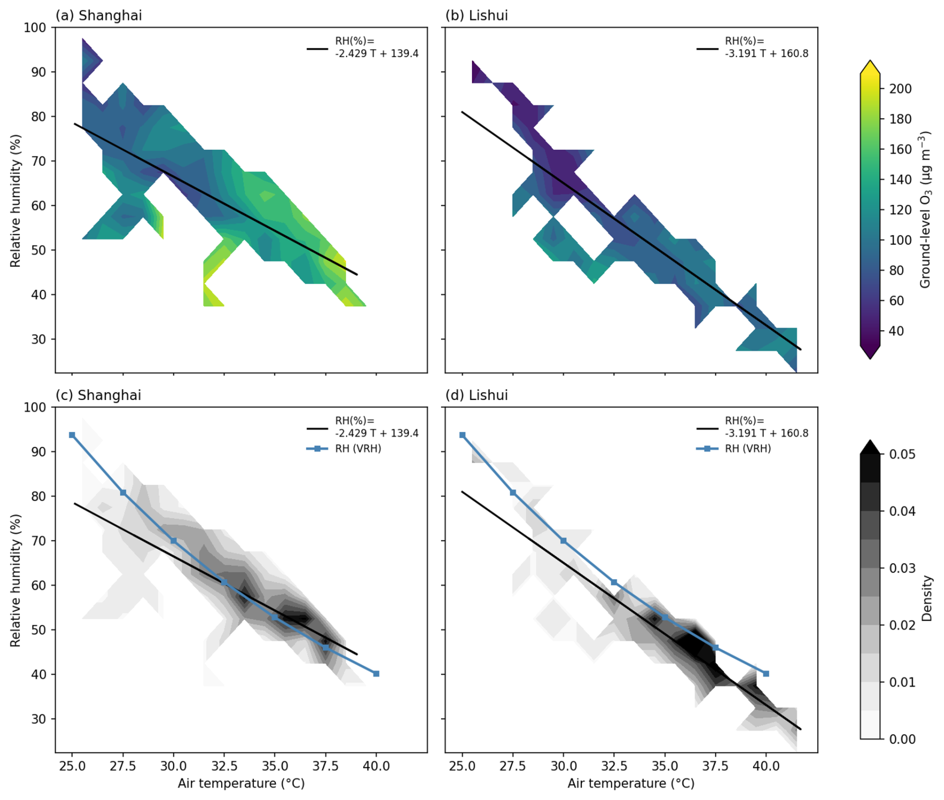
Figure 5 Observed air temperature-relative humidity space for (a, c) Shanghai and (b, d) Lishui (daytime, T≥25 °C), Panels (a)–(b) show the ground-level O₃ (µg m⁻³) binned on a 1 °C × 5 % RH grid; panels (c)–(d) show the data density (fraction of site samples per bin) on the same grid. The solid black line in each panel is the ordinary-least-squares fit of RH to T from the unbinned 3-hourly records. Ozone: hourly observations averaged from 8 AQMS (Shanghai) and 3 AQMS (Lishui); meteorology: three-hourly MMS data; all aggregated to 3 h means. The blue solid line with square markers in panels (c)–(d) is the RH curve with conserved absolute humidity (q=0.0184 kg kg⁻¹) used in the VRH model scenario.

In both regions, RH decreases systematically with warming. In Shanghai, the typical RH spread within a given temperature bin is about 20 % (e.g. 45 %–65 % at 35 °C), with larger variability at lower T and progressively narrower ranges at higher T (Fig. 5c). Lishui shows a similar tendency, with most samples concentrated between 32–37 °C and 35 %–55 % RH (Fig. 5d). Across the observed T-RH space, O₃ increases with temperature and decreases with RH, indicating a preference for warm, dry conditions.

Linear regression of RH on T yields slopes of −2.429 % °C⁻¹ for Shanghai and −3.191 % °C⁻¹ for Lishui (p<0.01 in both cases). The weaker slope in Shanghai, together with its narrower T range, is consistent with the moderating influence of sea-land thermal and moisture exchanges on coastal boundary-layer conditions, whereas the steeper slope in Lishui reflects a greater propensity for hot-dry excursions in a forested inland setting. The RH-T co-variation is much tighter in Shanghai (R²=0.83) than in Lishui (R²=0.57): in Shanghai the highest-density region (Fig. 5c) and the strongest O₃ increases (Fig. 5a) lie close to the regression line, implying that the linear T-RH relationship provides a good description of typical warm-season daytime conditions and of the pathway along which O₃ responds to combined warming and drying. In Lishui, by contrast, the main density maximum lies above the regression line and does not coincide with the dominant O₃-increase pathway, indicating that the fitted slope is influenced by a smaller number of hot, anomalously dry episodes. This behaviour is consistent with previous studies reporting that Lishui RH conditions are dominated by strong evapotranspiration from vegetation and soils, which is negatively correlated with temperature over the YRD in summer (Wang et al., 2023). In addition, stomatal closure under low-humidity conditions, which always corresponds to high-temperature conditions, would reduce O₃ dry deposition and further enhance O₃ levels (Kavassalis and Murphy, 2017), contributing to the high-O₃ tail at the hot, dry end of the Lishui distribution.

In Fig. 5c and d, we compare relative humidity from the VRH model configuration used in the subsequent simulations – defined by a conserved absolute humidity equal to the regional JJA 2022 mean (q=0.0184 kg kg⁻¹) – with the observed T-RH distribution. The VRH curve follows the locus of highest observational density in both Shanghai and Lishui, indicating that this configuration provides a realistic representation of the humidity-temperature conditions sampled in 2022 and is therefore suitable as the baseline humidity scenario for the box-model experiments.

Overall, Fig. 5 demonstrates that hot, dry conditions are favourable for elevated O₃ at both sites, but that the joint T-RH-O₃ variability differs between the coastal megacity and the forest-surrounded inland region: Shanghai exhibits a stronger, more coherent O₃-T-RH relationship in summer 2022 than Lishui, reflecting differences in local meteorology, surface characteristics, precursor emissions and chemical regime.

To interpret these observed O₃-temperature-humidity relationships in terms of process contributions and mechanisms, we next use an observation-constrained box model to quantify the extent to which the observed high-temperature O₃ response can be explained by changes in local chemical kinetics, precursor abundances, temperature diurnal cycles, and humidity conditions. Furthermore, the mechanisms underlying process contributions will be explored through budget-level simulations.

3.2 Chemical-regime diagnosis and process consistency of the box model

This section evaluates whether the UKCA Box model provides chemically plausible Shanghai-like and Lishui-like environments for the subsequent temperature-sensitivity experiments. The purpose is not to perform a formal model evaluation against observations or to use UKESM as an observational benchmark. Instead, we use three complementary diagnostics: (i) local O₃ responses to perturbations in NO_x and VOC emissions, (ii) contextual comparison of selected short-lived chemical species with available observations, and (iii) comparison of O_x production and loss pathways between the box model and the same-chemistry UKESM-AMIP simulation.

To establish the precursor-sensitivity regimes underlying the subsequent O₃-temperature analysis, Fig. 6 examines the O₃ response to NO_x and VOC changes using O₃-NO_x-isoprene response surfaces at 30 °C and ±10 % precursor perturbations across 25 to 40 °C.

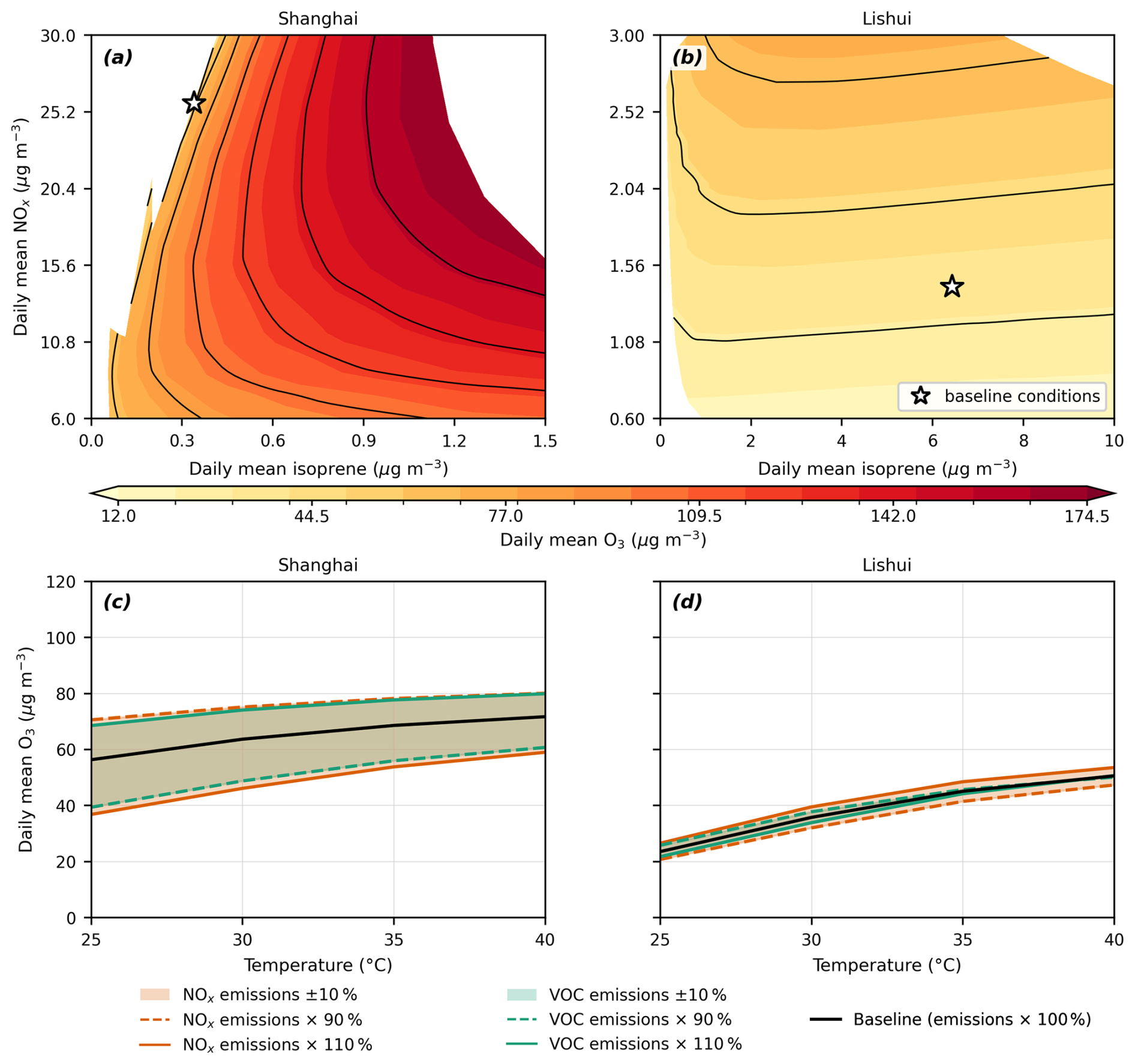
Figure 6 Simulated precursor sensitivity of daily mean surface O₃ in Shanghai and Lishui using the UKCA Box Model under the VRH_Ori baseline configuration with emission changes. Panels (a) and (b) show box model simulations of the evolution of ozone as a function of NO_x (NO+NO₂) and isoprene at 30 °C. Colours indicate daily mean O₃, black lines denote O₃ contours, and white stars mark the baseline conditions. Panels (c) and (d) show the temperature dependence of O₃ under ±10 % perturbations in NO_x and VOC emissions at 25, 30, 35, and 40 °C.

Figure 6 summarises the box-model sensitivity experiments used to diagnose precursor regimes in Shanghai (Fig. 6a and c) and Lishui (Fig. 6b and d). The baseline experiments, where there are no other processes but chemical reaction rates and pathways changing with temperature (marked as Ori), are consistent with the observed conditions in the 28.75–31.25 °C temperature bin. In Shanghai, the daily-mean O₃ is 63.7 µg m⁻³ in the model versus 69.5 µg m⁻³ in the observations. In Lishui, the corresponding values are 35.8 µg m⁻³ (model) and 52.5 µg m⁻³ (observations), a low bias that is consistent with Lishui being NO_x-limited (see below) and suggests that the grid-cell-average NO_x levels in the box configuration are lower than those sampled by the monitoring site.

Panels (a) and (b) show the simulated O₃ response surfaces in NO_x-isoprene concentration space at 30 °C for Shanghai and Lishui, respectively. The Shanghai baseline lies within a VOC-limited regime, where O₃ increases with isoprene and decreases with increasing NO_x. In contrast, the Lishui baseline lies within a NO_x-limited regime, where O₃ responds positively to NO_x and only weakly to additional isoprene.

The local ±10 % perturbations show consistent precursor responses across the investigated temperature range. In Shanghai (Fig. 6c), O₃ decreases with higher NO_x emissions and increases with higher VOC emissions from 25 to 40 °C, indicating a VOC-limited regime (Pusede et al., 2015). This VOC-limited behaviour is consistent with the high-NO_x, anthropogenically dominated environment of Shanghai and agrees with Liu et al. (2021b)'s study on the effectiveness of emission control strategies in China's major urban areas. In contrast, Lishui (Fig. 6d) exhibits the opposite tendency: O₃ increases with NO_x enhancement and is only weakly affected by VOC perturbations, signifying a NO_x-limited regime (Utembe et al., 2018). This behaviour is characteristic of rural or suburban photochemical environments influenced by regional BVOC emissions and relatively low NO_x levels (Sillman, 1999).

The signs of these responses remain unchanged between 25 and 40 °C, indicating no regime reversal within the tested perturbation range. These experiments therefore establish contrasting VOC-limited and NO_x-limited baseline environments for interpreting the subsequent O₃-temperature and O_x budget analyses.

The simulated PAN, OH, HO₂, and C₅H₈ concentrations are compared with the available observational references in Table 4.

Table 4 Comparison of PAN, OH, HO₂, and C₅H₈ levels in observation and UKCA Box Model.

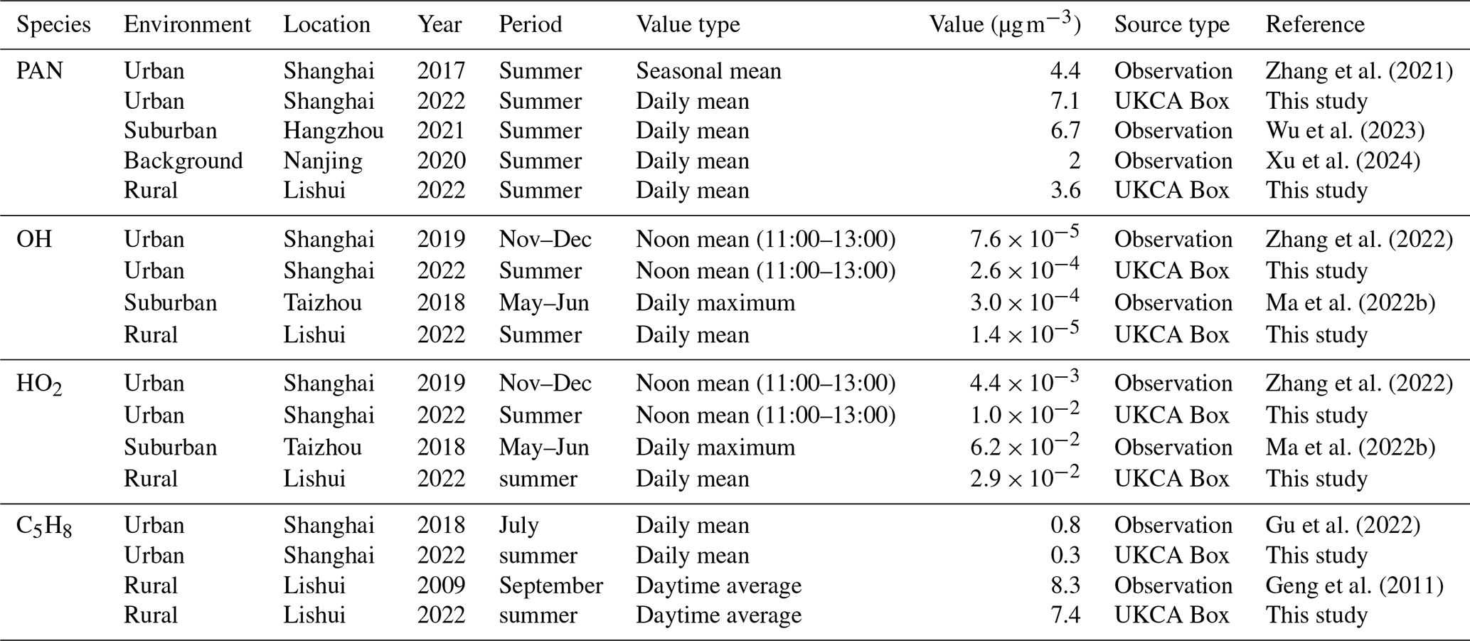
The model values in Table 4 are from baseline experiments (Ori) at 30 °C. The simulated PAN and C₅H₈ concentrations are consistent in order of magnitude with the reported observations. Direct summertime OH and HO₂ measurements are not available for urban Shanghai, so the winter Shanghai measurements provide the closest direct urban reference. Same-site measurements in other cities show that daytime OH is approximately 2–5 times higher in summer than in winter, while the summer-to-winter difference in HO₂ ranges from little seasonal change to a factor of approximately 5 (Heard et al., 2004; Kanaya et al., 2007; Ren et al., 2006). The Shanghai observations therefore provide a well-defined urban reference for the magnitude of HO_x, while the Taizhou measurements provide the corresponding warm-season YRD comparison.

The corresponding O_x production and loss pathways in the UKCA Box model and UKESM-AMIP are compared in Fig. 7.

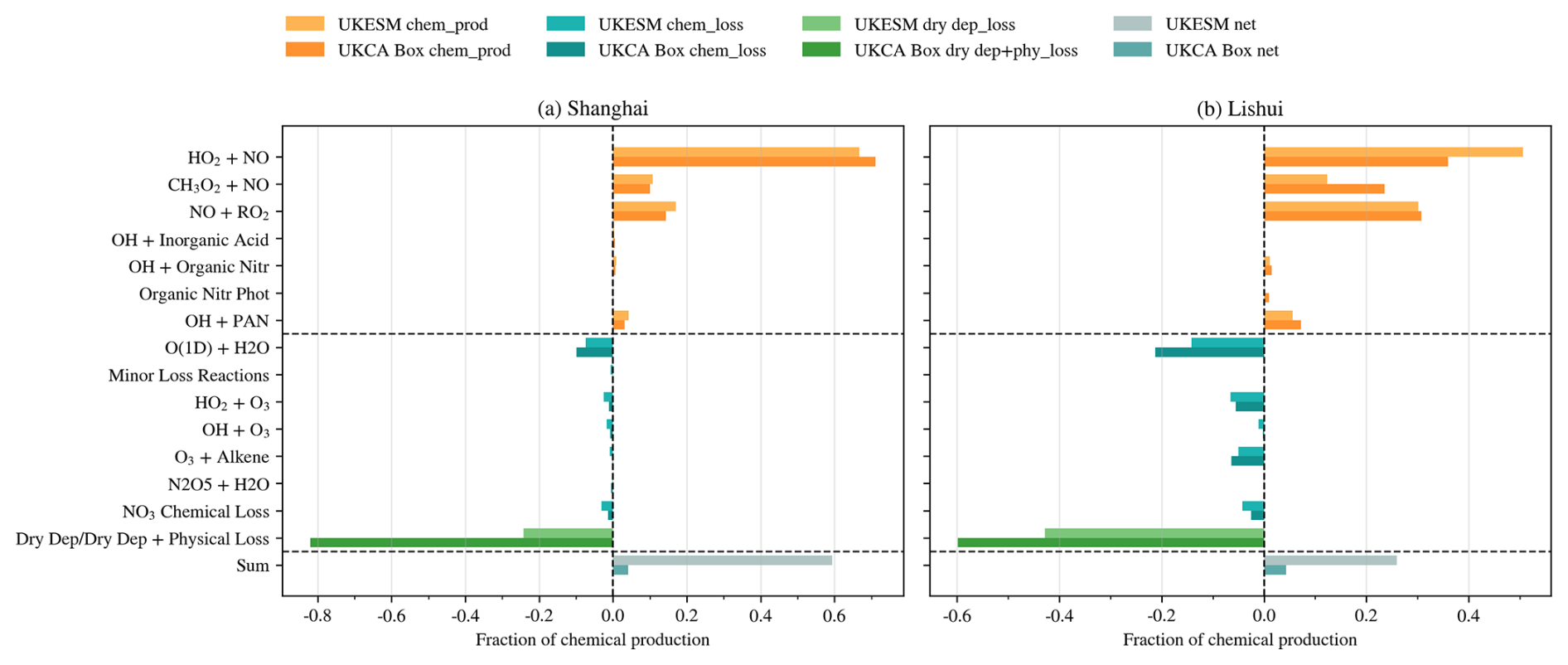
Figure 7 O_x production-loss budget by process category for two models at two sites. Panels (a)–(b) show the fractional contribution to total chemical production (unitless) from each reaction class. Positive bars denote chemical production (orange tones), negative bars denote chemical loss (teal tones) and dry deposition (UKESM) $/$ dry deposition + physical transport (UKCA Box) loss (green tones); the grey bar at the far right gives the net sum. Darker shades represent UKESM and lighter shades the UKCA Box. Reaction classes on the y axis include major O_x production and loss pathways. (a) Shanghai; (b) Lishui. Box model simulations were conducted under baseline conditions (Ori settings, 30 °C, and 70 % RH). The JJA averaged temperature and humidity in UKESM are 27.1 °C and 71.9 % RH.

Figure 7 compares the fractional O_x production and loss pathways in the UKCA Box model with those simulated by UKESM-AMIP using the same UKCA chemical mechanism. The UKESM-AMIP simulation is used as a three-dimensional context for interpreting the box-model O_x budget, because it includes physical processes that are absent from the 0-D box configuration, such as transport, boundary-layer mixing, convection, and meteorological variability.

The Box Model reproduces the rank order of production pathways in the nudged UKESM-AMIP model. In Shanghai, the total O_x production flux is $\mathrm{1.62}\times {\mathrm{10}}^{-\mathrm{9}}$ $\mathrm{kg}{\mathrm{m}}^{-\mathrm{2}}{\mathrm{s}}^{-\mathrm{1}}$ in the Box model versus $\mathrm{2.03}\times {\mathrm{10}}^{-\mathrm{9}}$ $\mathrm{kg}{\mathrm{m}}^{-\mathrm{2}}{\mathrm{s}}^{-\mathrm{1}}$ in the UKESM model. And in Lishui, this O_x production flux is $\mathrm{4.10}\times {\mathrm{10}}^{-\mathrm{10}}$ $\mathrm{kg}{\mathrm{m}}^{-\mathrm{2}}{\mathrm{s}}^{-\mathrm{1}}$ in the Box model, while this value is $\mathrm{8.40}\times {\mathrm{10}}^{-\mathrm{10}}$ $\mathrm{kg}{\mathrm{m}}^{-\mathrm{2}}{\mathrm{s}}^{-\mathrm{1}}$ in the UKESM.

In both cities, peroxy-NO reactions (HO₂+NO and ${\mathrm{RO}}_{\mathrm{2}}/{\mathrm{CH}}_{\mathrm{3}}{\mathrm{O}}_{\mathrm{2}}+\mathrm{NO}$) dominate the chemical production fraction in the box model, matching the pattern in UKESM and consistent with summertime O₃ photochemistry described by Ma et al. (2022b). This agreement in fractional chemistry indicates that the box model captures the regime (NO_x-VOC-OH coupling) rather than simply tuning totals. Chemical loss through $\mathrm{O}{(}^{\mathrm{1}}\mathrm{D})+{\mathrm{H}}_{\mathrm{2}}\mathrm{O}\to \mathrm{2}\mathrm{OH}$ and radical-ozone reactions (HO₂+O₃, OH+O₃) is represented with similar sign and relative importance in both frameworks.

The UKCA Box simulation shows a larger fractional contribution from dry deposition to the O_x sink (Fig. 7a–b). In the 3-D UKESM simulations, this sink is explicitly divided into deposition and dynamical export (dynamical export refers to physical transport and mixing, including horizontal advection, vertical entrainment with the growing boundary layer, shallow/deep convection, and ventilating outflow; not included in Fig. 7). In contrast, the box model treats the air parcel as a closed, well-mixed volume with no transport, so all non-chemical removal must appear as a lower-boundary deposition term. According to the monthly mean O₃ levels from June to August (UKESM) and the trend of daily mean O₃ levels (UKCA box model), both UKESM and UKCA Box produce nearly constant surface O₃, indicating that the net O_x tendency is close to zero. In UKESM, this large residual (“UKESM sum”) reflects the contribution of dynamical export. In the box model, the production-loss balance is achieved by having chemical production intentionally offset by the parameterised dry-deposition term, leaving only a small net production or loss. The larger deposition fraction in UKCA Box should therefore be interpreted as representing the combined effect of true surface uptake and the export processes, which are explicitly resolved in UKESM.

Overall, Fig. 6, Table 4, and Fig. 7 support the use of the UKCA Box model as a controlled chemical-process diagnostic. The model reproduces the expected contrast between a VOC-sensitive Shanghai-like environment and a NO_x-sensitive Lishui-like environment, and its dominant O_x production and loss pathways are broadly consistent with the same-chemistry UKESM simulation, while the differences illustrate the impact of absent physical drivers in the Box model. At the same time, the comparison does not constitute a formal validation of absolute O₃ concentrations, especially for Lishui, where monitoring-site observations and the regional box-model environment represent different spatial scales. The following sections therefore interpret the box-model experiments primarily in terms of relative process sensitivity and chemical-regime behaviour, rather than as direct simulations of monitored O₃ concentrations.

3.3 Temperature responses of ozone in the box model and observations

The observed and simulated O_3max–T_max relationships are compared in Fig. 8.

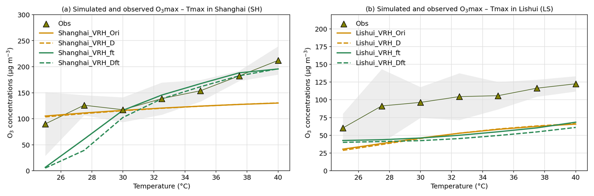
Figure 8 Comparison of observed and simulated O_3max–T_max relationships for (a) Shanghai and (b) Lishui (summer, JJA). Observations are shown as olive triangles connected by a line; the grey envelope denotes the 95 % confidence interval of the observed bin means (2.5 °C T_max bins; e.g., the 25 °C bin denotes summer days with T_max 23.75–26.25 °C). Colored solid/dashed lines show the four model configurations (VRH_Ori, VRH_D, VRH_ft, VRH_Dft; see Table 3).

Figure 8 compares observed JJA O_3max–T_max relationships in the VRH set of experiments with the UKCA Box Model: Ori (reference – fixed temperature and isoprene emissions across all hours of day), D (diurnal temperature cycle only), ft (temperature-dependent isoprene only), and Dft (both). The main purpose of these sensitivity experiments is to evaluate the impact of those processes on O₃'s temperature responses. In the box model simulations, the VRH experiments exhibit a trend in RH-temperature that resembles reality; thus, these experiments are considered reasonably good evaluators of the box model's performance when compared with observations.

Shanghai (urban; Fig. 8a). Above 30 °C, the ft and Dft simulations exhibit significant coordination in both ozone concentrations and trend, indicating that the temperature dependence of isoprene emissions explains most of the observed sensitivity in this regime. Relative to Ori and D, both ft and Dft lift O₃ by about 20 to 40 µg m⁻³ at 32.5–37.5 °C and reproduce the monotonic increase with temperature. At T < 30 °C, observations align more closely with Ori/D, whereas ft/Dft are low-biased. Two factors likely contribute: (i) wider uncertainty at the cool end (grey 95 % CI band) owing to fewer low-temperature days in summer 2022, and (ii) meteorological controls (e.g., mixing depth, advection, cloudiness) that covary with temperature but are not explicitly represented in the box model, which isolates chemical responses. At the upper tail, the simulated slope weakens because the applied isoprene function saturates at ∼38.3 °C, reducing the Dft (and ft) response from 9.3 $\mathrm{\mu }\mathrm{g}{\mathrm{m}}^{-\mathrm{3}}\mathrm{°}{\mathrm{C}}^{-\mathrm{1}}$ between 35–37.5 °C to 2.1 $\mathrm{\mu }\mathrm{g}{\mathrm{m}}^{-\mathrm{3}}\mathrm{°}{\mathrm{C}}^{-\mathrm{1}}$ between 37.5–40 °C; the observations maintain a steeper gradient (≈ 12 $\mathrm{\mu }\mathrm{g}{\mathrm{m}}^{-\mathrm{3}}\mathrm{°}{\mathrm{C}}^{-\mathrm{1}}$). The different isoprene emission threshold might be the cause, since suppression of isoprene emissions was not observed in the 10–40 °C range in Shanghai (Gu et al., 2022). And additional heat-linked processes (e.g., boundary-layer dynamics, anthropogenic VOCs, or NO_x variability) may continue to amplify O₃ at extreme temperatures.

Lishui (rural; Fig. 8b). The simulations reproduce the shape of the observed O₃-T curve, but the simulated O₃ is systematically low-biased by about 50 µg m⁻³. This offset is consistent with site representativeness (i.e. the observations exhibit a populated area in Lishui where NO_x emissions are higher than the box model simulations, which cover the whole Lishui region, most of which are rural areas). Importantly, introducing temperature-dependent isoprene (ft/Dft) yields only minor changes relative to Ori/D, indicating that Lishui operates largely in a NO_x-limited regime where additional VOC reactivity produces only modest O₃ increases, i.e. including T-dependence for isoprene leads to higher VOC levels, but this doesn't increase O₃ in Lishui, whereas it does in Shanghai. The small influence of the D option confirms that, after binning by T_max, imposing a diurnal temperature cycle alone does not substantially alter daily O_3max in this case.

Overall, the VRH experiments show that the UKCA Box captures the observed temperature sensitivity of O₃ when the isoprene-temperature coupling is represented (Shanghai), while the weak ft/Dft effect at Lishui is consistent with NO_x limitation. Discrepancies at low temperatures and in the highest bins highlight the role of meteorology and extreme-heat processes that lie outside the box configuration, motivating targeted sensitivity tests (e.g., boundary-layer depth, deposition, NO_x variability) in future work.

The resulting changes in O_3max between 30 and 40 °C are quantified in Table 5.

Table 5 Changes in daily maximum O₃ (ΔO_3max) from 30 to 40 °C. Unit: µg m⁻³.

Table 5 presents the increase in O_3max from 30 to 40 °C for the observations and the box model experiments. Because the experiments differ only in the process switched on, we quantify each process's contribution to the O₃ warming response by comparing the simulated 30 to 40 °C change. For each experiment X, we define ΔO${}_{\mathrm{3}}^X$ = O${}_{\mathrm{3}}^X$(40 °C) − O${}_{\mathrm{3}}^X$ (30 °C), and similarly, ΔO${}_{\mathrm{3}}^{\mathrm{obs}}$ from the observations. All metrics below are expressed as fractions of ΔO${}_{\mathrm{3}}^{\mathrm{obs}}$ and therefore dimensionless. The net chemical response is $f_{\mathrm{chem}}=\mathrm{\Delta }{{\mathrm{O}}_{\mathrm{3}}}^{\mathrm{VRH}\mathrm{\_}\mathrm{Ori}}/\mathrm{\Delta }{{\mathrm{O}}_{\mathrm{3}}}^{\mathrm{obs}}$, i.e., the fraction of the observed 30 to 40 °C increase that can be explained by temperature-dependent gas-phase chemistry alone under VRH conditions. The additional effect of each process is then quantified as the incremental fraction of ΔO${}_{\mathrm{3}}^{\mathrm{obs}}$ gained when that process is switched on: for the diurnal cycle, $f_{\mathrm{diurnal}}=(\mathrm{\Delta }{{\mathrm{O}}_{\mathrm{3}}}^{\mathrm{VRH}\mathrm{\_}\mathrm{D}}-\mathrm{\Delta }{{\mathrm{O}}_{\mathrm{3}}}^{\mathrm{VRH}\mathrm{\_}\mathrm{Ori}})/\mathrm{\Delta }{{\mathrm{O}}_{\mathrm{3}}}^{\mathrm{obs}}$; for the isoprene temperature dependence, $f_{\mathrm{iso}}=(\mathrm{\Delta }{{\mathrm{O}}_{\mathrm{3}}}^{\mathrm{VRH}\mathrm{\_}\mathrm{ft}}-\mathrm{\Delta }{{\mathrm{O}}_{\mathrm{3}}}^{\mathrm{VRH}\mathrm{\_}\mathrm{Ori}})/\mathrm{\Delta }{{\mathrm{O}}_{\mathrm{3}}}^{\mathrm{obs}}$; and for humidity, $f_{\mathrm{humid}}=(\mathrm{\Delta }{{\mathrm{O}}_{\mathrm{3}}}^{\mathrm{FRH}}-\mathrm{\Delta }{{\mathrm{O}}_{\mathrm{3}}}^{\mathrm{VRH}})/\mathrm{\Delta }{{\mathrm{O}}_{\mathrm{3}}}^{\mathrm{obs}}$. Positive values indicate that the process amplifies the increase in O₃ with temperature, whereas negative values indicate damping. This normalisation allows us to directly compare the extent to which the observed O₃-temperature sensitivity can be attributed to each process at the two sites. Notably, due to the nature of the 0-D box-model (no transport, clouds, or physical feedbacks), this attribution should be interpreted as under a controlled chemical framework instead of a full decomposition of all meteorological controls.

In Shanghai, decomposition of the O_x budget shows that the net chemical term accounts for 18.7 % of the observed 30 to 40 °C increase, while the diurnal temperature cycle alone has a negligible effect on the net chemistry. By contrast, the temperature dependence of isoprene emissions explains 69.1 % of the observed O₃ rise, identifying this pathway as the dominant driver of the warm-season O₃-T slope in urban Shanghai. When isoprene's temperature sensitivity is enabled, the diurnal cycle yields an additional 14.3 % O₃ increment, consistent with enhanced photolysis and radical propagation during warmer, sunnier hours reported in YRD (Xia et al., 2022).

Humidity acts as an important modulator of the O₃-temperature response. In our experiments, increasing RH by about 30 % at 40 °C (FRH: q=0.0320 kg kg⁻¹, RH = 70 %; VRH: q=0.0184 kg kg⁻¹, RH = 40.2 %), while keeping the temperature diurnal cycle and isoprene temperature dependence switched on (VRH_Dft settings), leads to a 21.9 µg m⁻³ reduction in O_3max at 40 °C. Expressed as a fraction of the observed 30 to 40 °C change, this contribution is (ΔO${}_{\mathrm{3}}^{\mathrm{FRH}\mathrm{\_}\mathrm{Dft}}-\mathrm{\Delta }{{\mathrm{O}}_{\mathrm{3}}}^{\mathrm{VRH}\mathrm{\_}\mathrm{Dft}})/\mathrm{\Delta }{{\mathrm{O}}_{\mathrm{3}}}^{\mathrm{obs}}$. This humidity-driven decrease reflects the role of water vapour in enhancing O_x loss via O(¹D)+H₂O pathway: in the FRH case, the vertically integrated O(¹D)+H₂O flux (kg m⁻² s⁻¹) increases by about 42 %, strengthening the O₃ decomposition pathway and offsetting part of the thermally driven O₃ enhancement.

In the NO_x-limited regime (i.e. Lishui), the process attribution gives different results. The chemical response itself explains 80.4 % of the observed 30 → 40 °C change, implying that enhanced photochemistry at higher temperatures – through faster reaction rates and stronger actinic flux – dominates the O₃ increase (Archibald et al., 2020b). The isoprene temperature dependence contributes only 10.4 %, consistent with a NO_x-limited environment where additional VOC reactivity produces comparatively small changes in O₃ production (Steiner et al., 2006). The diurnal temperature cycle makes only a minor contribution to the 30 → 40 °C O₃ increase, whereas the humidity perturbation is non-negligible. When RH is raised from 40.2 % to 70 % at 40 °C (VRH: q=0.0184 kg kg⁻¹; FRH: q=0.0320 kg kg⁻¹) under the VRH_Dft settings, the resulting change in humidity accounts for 9.1 µg m⁻³ of O_3max reduction. O_x budget diagnostics show that this damping arises from two linked effects of higher water vapour: a reduction in O_x production via the HO₂+NO channel (≈15.3 % reduction in FRH scenarios compared with that in VRH scenarios), and an enhancement of O_x loss via O₃ photolysis followed by O(¹D)+H₂O (≈36.9 % compared with VRH scenarios). Both mechanisms are consistent with Li et al. (2021), who showed that elevated relative humidity suppresses O₃ generation by inhibiting the OH/HO₂-NO₂ chain and promotes O₃ loss through the O(¹D) + H₂O pathway.

Taken together, Fig. 8 and Table 5 demonstrate that the UKCA Box model produces a physically interpretable decomposition of the O₃-temperature relationship: isoprene-temperature coupling is decisive in Shanghai, while baseline chemical partitioning and humidity dominate in Lishui. These site-specific attributions align with the contrasting chemical regimes and underscore the need to represent both biogenic VOC responses and meteorologically linked processes when projecting O₃ extremes under warming.

3.4 Temperature response on O_x, PAN, and HO_x diurnal cycles

The temperature dependence of the O_x budget is examined through its diurnal evolution in Fig. 9 and the corresponding daily integrated production and loss terms in Table 6.

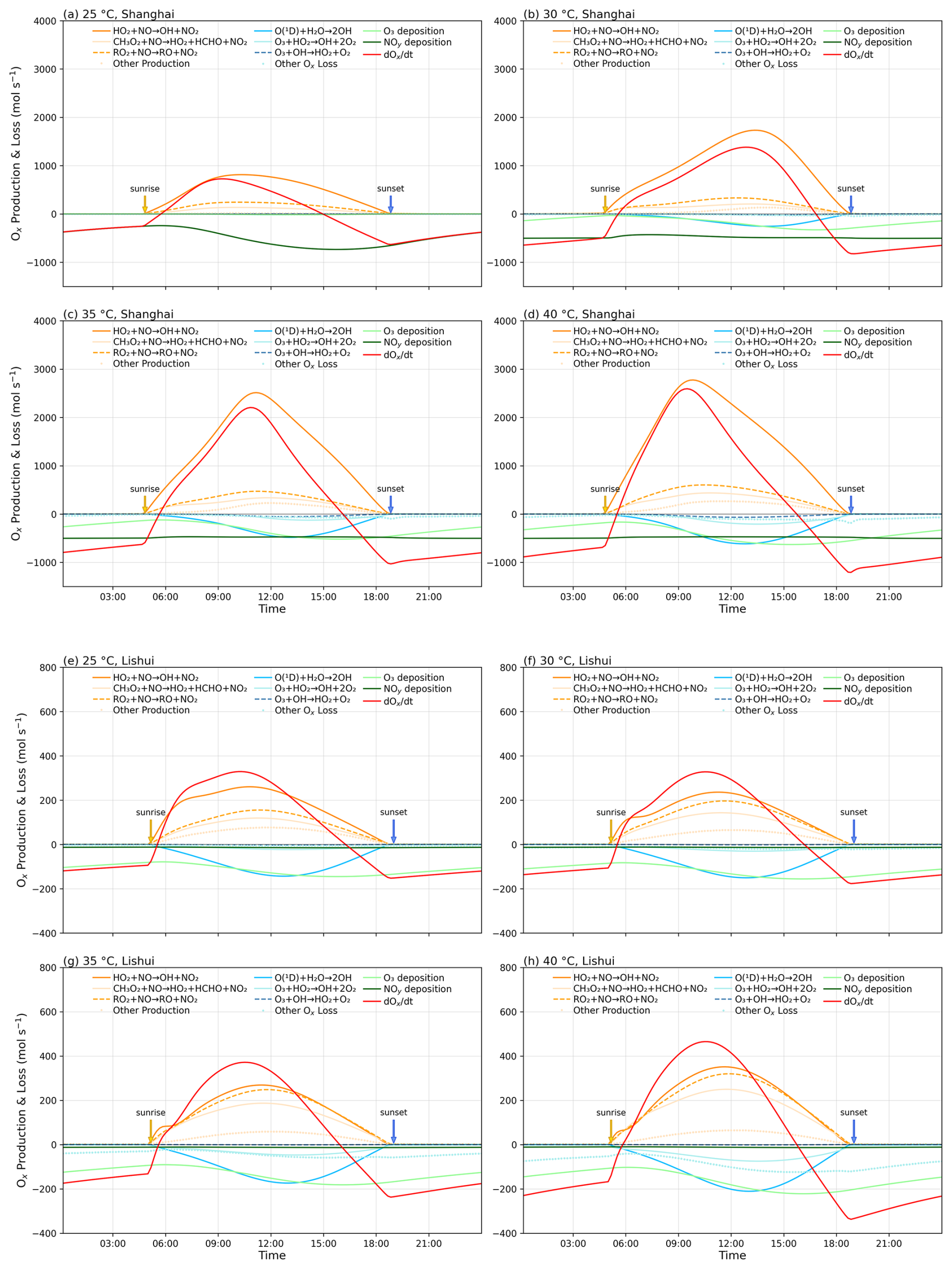
Figure 9 Diurnal O_x budget in the Dft configuration for Shanghai at T_max of (a) 25 °C, (b) 30 °C, (c) 35 °C, (d) 40 °C, and for Lishui at T_max of (e) 25 °C, (f) 30 °C, (g) 35 °C, (h) 40 °C. Curves show major chemical production pathways (orange), chemical loss terms (blue), deposition loss terms (green), and the net tendency $\mathrm{d}{\mathrm{O}}_x/\mathrm{d}t$ (red). Arrows indicate local sunrise and sunset. Time is local, and budget terms are expressed in mol s⁻¹. The y axis scale is consistent within each site but differs between Shanghai and Lishui.

Table 6 Daily contribution of main production and loss pathways to the O_x budget at 25, 30, 35, and 40 °C in Shanghai (unit: metric tonnes of O_x per day (t O_x d⁻¹; O_x counted as O₃).

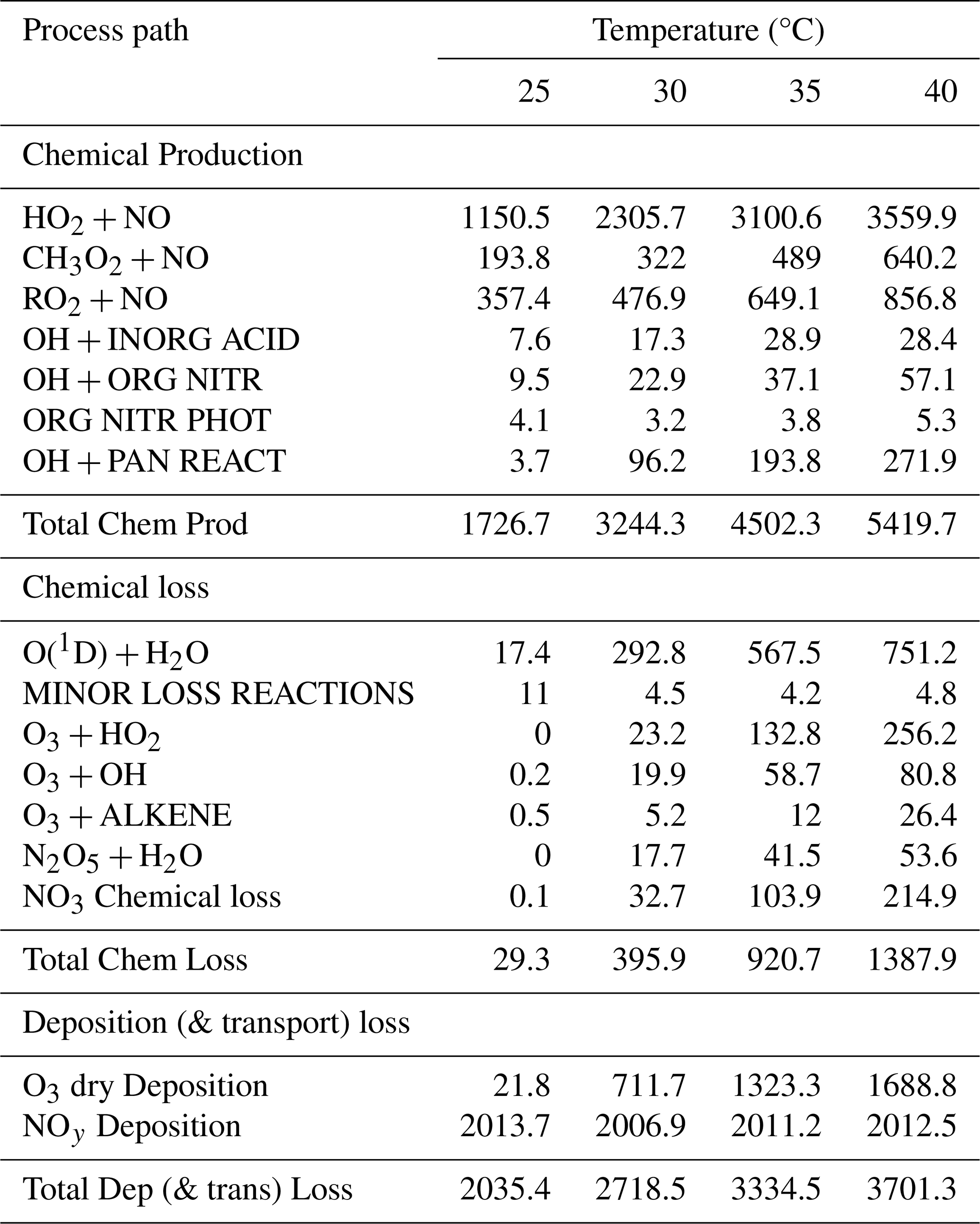
Table 7 Daily contribution of main production and loss pathways to the O_x budget at 25, 30, 35, and 40 °C in Lishui (unit: metric tonnes of O_x per day (t O_x d⁻¹; O_x counted as O₃).

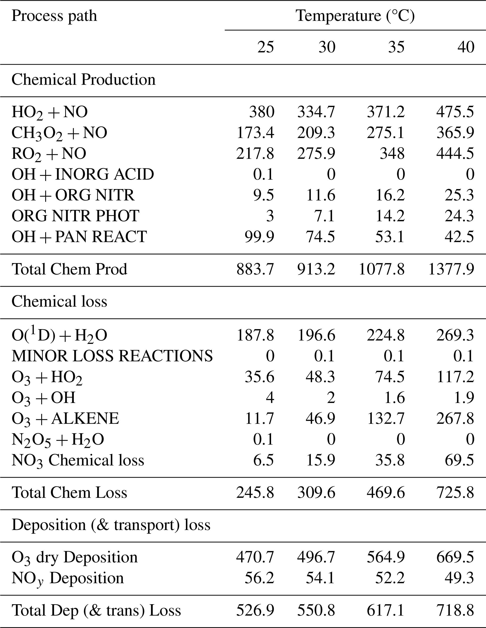
Figure 9, Tables 6 and 7 summarise how O_x production and loss terms from the UKCA Box Model respond to temperature. In Shanghai (Fig. 9a–d; Table 6), all major production pathways increase with temperature, except for organic-nitrate photolysis (labelled ORG NITR PHOT in Table 6), which has a minor impact on total production. From Fig. 9a–d, the reaction ${\mathrm{HO}}_{\mathrm{2}}+\mathrm{NO}\to \mathrm{OH}+{\mathrm{NO}}_{\mathrm{2}}$ is the dominant and most temperature-sensitive source of O_x production. Although its marginal sensitivity (change in O_x production per °C) weakens from 25 → 40 °C, it remains the single largest contributor. The second key source, ${\mathrm{RO}}_{\mathrm{2}}+\mathrm{NO}\to \mathrm{RO}+{\mathrm{NO}}_{\mathrm{2}}$, displays the opposite behaviour – its temperature sensitivity strengthens with warming. From 35 to 40 °C, the contribution of RO₂+NO to total O_x production increases by 207.7 t O_x d⁻¹ in Shanghai, nearly doubling the increase from 25 to 30 °C, underscoring the growing role of peroxy-radical chemistry at high temperatures. This growth is consistent with high-temperature partitioning of the OH-HO₂-RO₂ cycle – most notably the HO₂+NO channel – and with the well-documented increase in effective VOC reactivity under hot conditions due to both faster kinetics and temperature-sensitive VOC emissions (e.g. isoprene) (Meng et al., 2023). Even with reduced temperature sensitivity, the HO₂+NO reaction accounted for more than 50.1 % of total chemical production, confirming the importance of the HO₂-NO pathway in the urban regime.

For chemical loss in Shanghai, O(¹D) + H₂O → 2OH is the leading term. Its temperature sensitivity is 55.01 t O_x d⁻¹ °C⁻¹ between 25–35 °C, decreasing to ∼36.74 t O_x d⁻¹ °C⁻¹ from 35–40 °C, consistent with partial saturation of midday photolysis at the hottest conditions. In the total budget, however, deposition dominates loss. O₃ dry deposition exhibits the stronger temperature sensitivity, which maximises between 25–35 °C, whereas NO_y deposition varies less with temperature but remains the largest absolute sink at all temperatures, controlling the sign of the net O_x tendency. As deposition in the UKCA Box Model serves both as deposition and as physical loss, the magnitude comparison is not so useful.

In Lishui (Fig. 9e–h; Table 7), both production and loss magnitudes are substantially smaller than in Shanghai, consistent with lower precursor loadings in rural southwestern Zhejiang and the prevalence of NO_x-limited chemistry outside urban cores in the YRD (An et al., 2021; Ren et al., 2022). HO₂+NO is still the largest single production term, but at T>30 °C its strength becomes comparable to CH₃O₂+NO and RO₂+NO, indicating a more distributed peroxy-NO contribution in the regional background. For chemical loss, O(¹D) + H₂O dominates from 25–30 °C. At temperatures higher than 30 °C, O₃ + ALKENE reactions' contribution grows rapidly with temperature and becomes comparable in magnitude to O(¹D) + H₂O, highlighting the role of thermally enhanced VOC-ozone chemistry outside the urban core where the O₃+C₅H₈ reaction plays a crucial role. In the depositional budget, O₃ dry deposition is relatively more important in Lishui than in Shanghai, consistent with the much larger vegetated land fraction – which elevates deposition velocity of O₃ via stomatal and surface uptake – and with weaker in-situ NO_y production under rural low-NO_x conditions (Clifton et al., 2020a).

Overall, the Box model yields a coherent, process-level explanation for the observed O₃-temperature behaviour. In Shanghai, warming amplifies O_x primarily through HO₂+NO chemistry while deposition – especially NO_y deposition – limits the net build-up. In Lishui, the warming response is shared more evenly among peroxy-NO sources, and O₃ deposition plays a larger role in the sink, with O₃-alkene loss emerging at the hottest conditions.

To identify the role of PAN-mediated NO_x recycling, Fig. 10 shows the temperature dependence of PAN concentration and thermal decomposition at both sites.

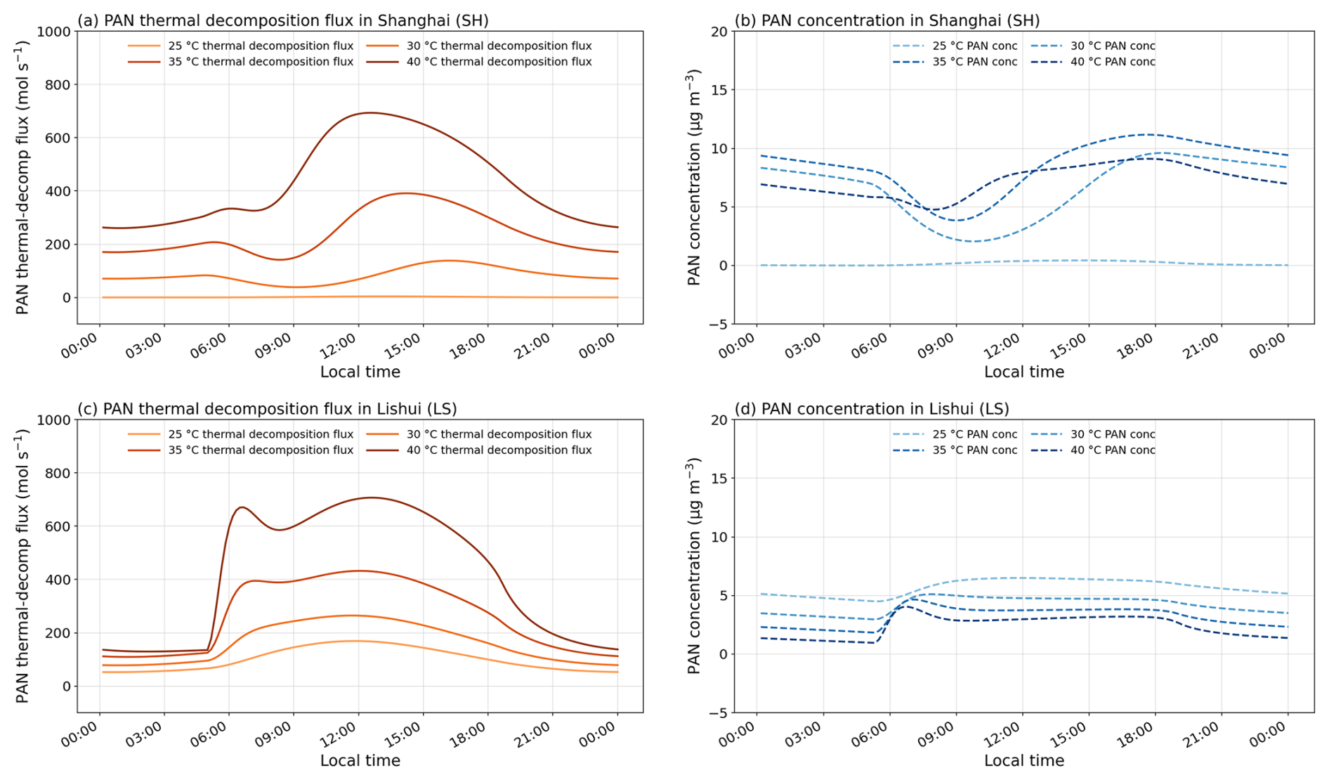
Figure 10 Diurnal peroxyacetyl nitrate (PAN) budget at four temperatures. (a–b) Shanghai and (c–d) Lishui. Solid orange curves show the PAN thermal-decomposition flux (left axis, mol s⁻¹); dashed blue curves show PAN concentration (right axis, µg m⁻³). Each pair corresponds to a temperature scenario (25, 30, 35, 40 °C; lighter → darker with increasing temperature). Local time on the x axis.

Figure 10 contrasts the diurnal evolution of peroxyacetyl nitrate (PAN) concentrations (dashed curves, right axis) with the thermal decomposition flux PAN → CH₃C(O)O₂ (PA) + NO₂ (solid curves, left axis) at four imposed temperatures in Shanghai (panel a) and Lishui (panel b). In both locations, the decomposition flux increases monotonically with temperature and peaks around local noon-early afternoon, with daytime values far exceeding nighttime values. This behaviour is consistent with the strong temperature dependence of the PAN stability (PAN thermally decomposes rapidly at higher temperatures) and with daytime heating that accelerates the decomposition reaction (Fischer et al., 2014).

Despite the broadly similar flux patterns, concentration responses differ by site. In Lishui (Fig. 10c–d), PAN concentrations decrease with warming across the full range. As the temperature rises, thermal loss outpaces daytime production (due to low ambient NO_x), so the reservoir is progressively depleted. The result is a clean negative PAN-T relationship.

In Shanghai, the response is non-monotonic. In Fig. 10b, from 25 to 35 °C, the PAN concentration increases, even as the thermal decomposition of PAN accelerates as shown in Fig. 10a. This implies that, over this range, enhanced PAN production – via larger peroxyacetyl radical supply and abundant NO₂ – offsets the faster loss, allowing concentrations to rise. However, at 40 °C, the pattern reverses after midday: the decomposition flux jumps sharply relative to 35 °C, while the PAN concentration drops in the afternoon. Two explanations, which are not mutually exclusive, are consistent with the curves. First, PAN's thermal instability means the PA + NO₂⇌ PAN equilibrium shifts strongly toward PAN dissociation at high temperature (Cleary et al., 2007); thermal loss is the primary PAN sink in the lower troposphere and accelerates through the warmest hours, producing the observed afternoon drawdown in Fig. 10a. Second, extreme heat coincides with lower afternoon PAN production efficiency, e.g. due to the reduction in biogenic precursor supply, e.g., C₅H₈ as an indirect source of PA encountered its threshold at 38.3 °C, or enhanced radical competition (Liu et al., 2021a; Ma et al., 2022a; Phillips et al., 2013), so low peroxyacetyl radical (PA) levels limit the reaction between PA + NO₂ to form PAN. This PAN concentration drop may imply a threshold of PAN thermal decomposition above 40 °C in Shanghai, which occurs above 39 °C in California as described by Steiner et al. (2010).

A further notable contrast is the lower temperature behaviour (25 °C). Both the thermal decomposition flux and the PAN concentration are lower in Shanghai than in Lishui at this temperature, indicating that, under cooler conditions, PAN acts as a less effective NO_x reservoir near the urban site.

Overall, Fig. 10 shows that warming consistently strengthens PAN thermal decomposition at both sites, but the net concentration response is site-specific: monotonic decreases in Lishui, and increases followed by depletion in Shanghai at the highest temperature. These distinctions have practical implications: during heat extremes, PAN-mediated transport of NO_x is likely reduced because rapid afternoon decomposition limits PAN lifetime in VOC-limited urban areas like Shanghai, and the effect can be less significant in Lishui.

The associated temperature responses of HO_x cycling and the HO₂+NO pathway are shown in Fig. 11.

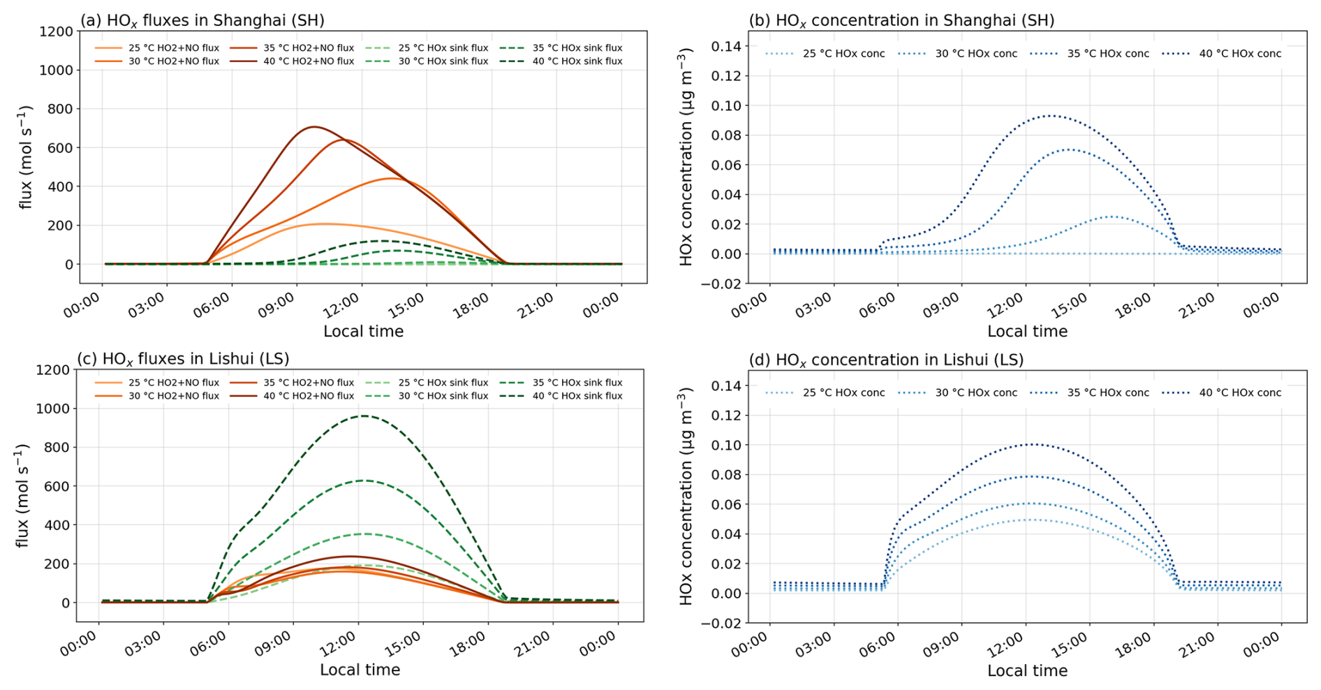
Figure 11 Diurnal HO₂+NO reaction, HO_x sink, and HO_x concentration at four temperatures. (a–b) Shanghai and (c–d) Lishui. Solid orange lines show the HO₂+NO reaction flux (left axis, mol s⁻¹); dashed green lines show the total HO_x sink flux (left axis); dotted blue lines show HO_x concentration (right axis, µg m⁻³). Each trio corresponds to a temperature scenario (25, 30, 35, 40 °C; lighter → darker with increasing temperature). Local time on the x axis.

Figure 11 presents the diurnal evolution of the HO₂+NO production flux (solid orange), the aggregate HO_x-termination (“sink”) flux (green dashed; e.g. $\mathrm{OH}+{\mathrm{NO}}_{\mathrm{2}}+M,{\mathrm{HO}}_{\mathrm{2}}+{\mathrm{RO}}_{\mathrm{2}}/{\mathrm{HO}}_{\mathrm{2}})$, and the HO_x concentration (blue dotted; right axis) at four imposed temperatures. As shown in Fig. 9, the HO₂ and NO reaction is the dominant O₃ chemical production pathway in both environments. HO_x sink reactions terminate O₃ formation, while HO_x is widely used as a proxy for the atmosphere's oxidising capacity, with OH controlling daytime oxidative processing (Feng et al., 2021); moreover, net ozone formation scales with the peroxy-NO reactions, so higher HO_x – especially HO₂ – correlates with stronger photochemical O₃ production (Archibald et al., 2020b; Pusede et al., 2015).

In both panels, chemical activity is tightly bound to daylight: fluxes are negligible at night, rise sharply after sunrise, peak near local noon-early afternoon, and collapse after sunset, reflecting the photochemical control of radical production.

In Shanghai (Fig. 11a–b), warming mainly strengthens the HO_x-driven O_x production. With increasing temperature, the daytime HO₂+NO production flux (solid curves) increases strongly, and the peak HO_x concentrations (blue dotted curves, right axis) also increase, indicating more efficient radical recycling and a faster O₃ production cycle at higher T. The HO_x termination flux (green dashed curves) also grows with temperature, but the enhancement remains much smaller than the HO₂+NO pathway throughout the day, so the temperature increase shows a more substantial impact on including more HO_x in O_x formation instead of facilitating the HO_x sink pathway. At T<30 °C, both HO_x levels and the sink are low, implying that primary radical production is weak and the O₃ production cycle can be slow.

In Lishui (Fig. 11c–d), the behaviour is significantly different. Across the temperature range, the HO_x sink plays a much larger role, and at T≥30 °C, its magnitude exceeds the HO₂+NO flux. Interpreted in the context of the O₃ chemical cycle, this means a larger fraction of the available HO_x is channelled into termination rather than propagation. Even so, HO_x concentrations remain high from 25 to 40 °C, indicating efficient radical production; the high sink simply prevents those radicals from translating into proportionally larger HO₂+NO rates.

Together, the panels show that warming enhances radical activity in both environments, but the partitioning between propagation and termination is site dependent: Shanghai exhibits production-dominated HO_x cycling that favours O₃ formation at high temperature, whereas Lishui exhibits sink-dominated cycling, consistent with background conditions where O₃ production is constrained by NO_x rather than HO_x availability.

4 Discussion

4.1 Potential influence of temperature-dependent AVOC emissions

The present UKCA Box configuration represents only a limited subset of emitted AVOCs. In particular, some alkanes, alkenes, and aromatic compounds associated with temperature-dependent evaporative emissions are not available as explicit emitted tracers in the current chemical mechanism. Incorporating the full range of temperature-dependent AVOCs would therefore require an extension of both the chemical mechanism and the emission mapping, and these species could not be included directly in the present box-model experiments.

To assess the potential importance of temperature-dependent AVOC emissions, we reproduced the temperature-dependent emission-scaling framework of Qin et al. (2025) using the JJA 2022 CEDS emissions for Shanghai. The calculation included selected AVOC categories associated with volatile chemical products (VCPs), including industrial and residential solvent use, and gasoline evaporation. Both temperature functions were normalised to 30 °C, which represents the average baseline condition used in the box-model experiments. From 30 to 40 °C, the selected VCP-related emission flux increased by 58.6 %, from $\mathrm{4.83}\times {\mathrm{10}}^{-\mathrm{10}}$ to $\mathrm{7.66}\times {\mathrm{10}}^{-\mathrm{10}}$ $\mathrm{kg}{\mathrm{m}}^{-\mathrm{2}}{\mathrm{s}}^{-\mathrm{1}}$, while the gasoline-evaporation flux increased by 33.3 %, from $\mathrm{4.17}\times {\mathrm{10}}^{-\mathrm{11}}$ to $\mathrm{5.56}\times {\mathrm{10}}^{-\mathrm{11}}$. The combined selected temperature-dependent AVOC flux consequently increased from $\mathrm{5.25}\times {\mathrm{10}}^{-\mathrm{10}}$ to $\mathrm{8.22}\times {\mathrm{10}}^{-\mathrm{10}}$ $\mathrm{kg}{\mathrm{m}}^{-\mathrm{2}}{\mathrm{s}}^{-\mathrm{1}}$, corresponding to an additional 56.6 % increase.

We further examined whether this estimated AVOC enhancement could be represented explicitly in the UKCA Box experiments by applying the CEDS-to-StratTrop lumping approach of Archer-Nicholls et al. (2021). Comparison of the relevant CEDS species and sectors with the emitted StratTrop AVOC tracers showed that the overlap is very limited. On the source-species mass basis used in the mapping, these species account for only 3.56 % of the selected gasoline-evaporation emissions, while none of the selected VCP-related solvent emissions is represented. Most of the temperature-dependent butanes, pentanes, higher alkanes, other alkenes and aromatics are therefore absent from the emitted-tracer mapping.

Qin et al. (2025) found that temperature-driven AVOC emission enhancements increased MDA8 O₃ by 4.6 ppb and peak O₃ by 7.5 ppb during a Shanghai heatwave. Their results indicate that an AVOC enhancement of the magnitude estimated here can produce a measurable additional O₃ increase under hot urban conditions. Temperature-dependent AVOCs can therefore increase anthropogenic VOC availability under hot urban conditions, and their resulting O₃ contribution will be examined using an expanded VOC mechanism in future work.

4.2 Influence of the isoprene temperature-response parameterisation

Because temperature-dependent isoprene emissions strongly amplify simulated O₃ in Shanghai, we examined how this effect depends on the emission scheme. We compared the JULES iBVOC formulation used in the main experiments with the temperature activity factor implemented in MEGAN v2.1. The iBVOC scheme used with JULES represents the short-term temperature response as $fT=min\left[\exp \right(\mathrm{0.1}(T-\mathrm{303.15})),\mathrm{2.3}]$. The response therefore increases exponentially above the 30 °C reference condition until reaching a fixed upper limit of 2.3 at approximately 38.3 °C, after which the emission factor remains constant (Pacifico et al., 2011). By contrast, the MEGAN temperature activity factor accounts for both the instantaneous temperature and thermal acclimation through the mean temperatures over the preceding 24 and 240 h, T24 and T240. These prior-temperature terms determine the magnitude and temperature of the emission maximum rather than imposing a fixed threshold (Guenther et al., 2012).

We examined the influence of these formulations in Shanghai by normalising both temperature factors to the same isoprene emission at 30 °C and applying them over the 30–40 °C experimental range. The JULES temperature factor increased from 1.0 at 30 °C to its maximum value of 2.3 above 38.3 °C. The MEGAN factor increased continuously throughout the investigated range, reaching 2.68 at 40 °C; under the T24 and T240 conditions (30 °C; assumed from JJA YRD conditions and model setting) applied here, its emission maximum therefore occurred above 40 °C and outside the experimental range. The corresponding isoprene flux at 40 °C was $\mathrm{2.92}\times {\mathrm{10}}^{-\mathrm{10}}$ $\mathrm{kg}{\mathrm{m}}^{-\mathrm{2}}{\mathrm{s}}^{-\mathrm{1}}$ using JULES and $\mathrm{3.40}\times {\mathrm{10}}^{-\mathrm{10}}$ $\mathrm{kg}{\mathrm{m}}^{-\mathrm{2}}{\mathrm{s}}^{-\mathrm{1}}$ using MEGAN, compared with the common value of $\mathrm{1.27}\times {\mathrm{10}}^{-\mathrm{10}}$ $\mathrm{kg}{\mathrm{m}}^{-\mathrm{2}}{\mathrm{s}}^{-\mathrm{1}}$ at 30 °C. These values correspond to increases of 130.0 % and 167.9 %, respectively.

The differences in calculated isoprene emissions propagated directly into the simulated evolution of daily maximum O₃. At 30 °C, both schemes produced the same daily maximum O₃ of 116.1 µg m⁻³. At 40 °C, daily maximum O₃ reached 199.3 µg m⁻³ with JULES and 212.3 µg m⁻³ with MEGAN. The resulting 30–40 °C increases were therefore 83.3 and 96.2 µg m⁻³, respectively. Differences between the schemes remained relatively small between 32.5 and 37.5 °C, but became more pronounced once the JULES temperature factor approached its fixed upper limit. At 40 °C, MEGAN produced 12.9 µg m⁻³ more O₃ than JULES. Thus, both schemes confirm a large isoprene-driven amplification of urban O₃ at high temperature, while the greater high-temperature response in MEGAN indicates that the fixed JULES threshold provides a more conservative estimate near and above 40 °C.

5 Summary and conclusions

This study quantitatively evaluated the summertime temperature responses of ground-level ozone (O₃) across the Yangtze River Delta (YRD) and diagnosed how temperature-dependent O_x chemistry modulates surface O₃ using targeted UKCA Box experiments. We combined site observations from the 2022 summer in an urban megacity (Shanghai) and a rural region (Lishui) with a suite of experiments that separated the roles of chemical kinetics, temperature-dependent biogenic emissions, diurnal thermal structure, and humidity. Furthermore, we examined the O_x budget, PAN thermolysis, and the HO_x cycle to identify the mechanisms underlying the observed temperature sensitivities. We highlight that urban-rural differences largely exist in the intensity, process, and mechanism of ground-level O₃ temperature responses. The conclusions are based on controlled 0-D box-model experiments, so the quantitative process fractions represent local chemical and emission-related sensitivities rather than a full meteorological attribution of the observed O₃-temperature relationship.

The principal regime-specific mechanisms identified by these analyses are summarised in Fig. 12, which contrasts typical summer (30 °C) and heat extreme (40 °C) conditions in Shanghai and Lishui. The conceptual comparison highlights the stronger temperature-amplified BVOC contribution in the Shanghai-like VOC-limited environment and the greater importance of radical-NO_x chemistry in the Lishui-like lower-NO_x environment, together with the modulation of both responses by humidity and diurnal temperature structure.

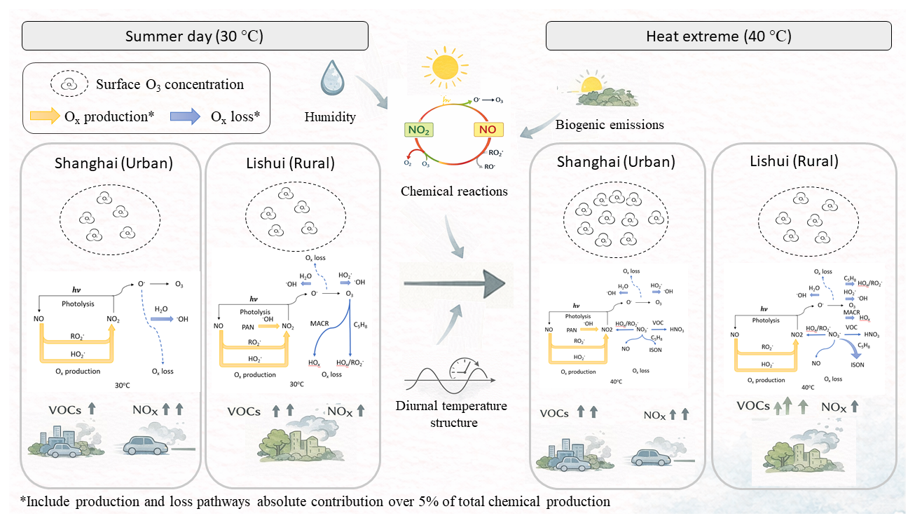
Figure 12 Conceptual summary of the mechanisms controlling surface ozone under typical summer conditions (30 °C; left) and heat extremes (40 °C; right) in Shanghai (urban) and Lishui (rural).

Summertime daily maximum observations showed robust, positive O₃-temperature relationships in both regions, stronger in Shanghai than in Lishui (mean JJA ΔO${}_{\mathrm{3}\max }-\mathrm{\Delta }{T}_{\max }=\mathrm{7.27}$ vs. 3.36 $\mathrm{\mu }\mathrm{g}{\mathrm{m}}^{-\mathrm{3}}\mathrm{°}{\mathrm{C}}^{-\mathrm{1}}$). Heatwave slopes remained positive in Lishui, but were statistically uncertain in Shanghai due to the limited number of events and larger variance at the low tail. Two-dimensional T-RH maps revealed that O₃ increases with temperature and decreases with relative humidity (RH). Because RH falls by ∼ 2.4 %–3.2 % RH per °C, part of the apparent temperature signal is mediated by drying.

Factorial experiments isolated (i) net temperature-dependent chemical effects (Ori), (ii) the diurnal temperature cycle (D), (iii) temperature-dependent isoprene emissions (ft), and (iv) their combination (Dft), under fixed- and variable-RH assumptions (FRH/VRH). Under the adopted isoprene-temperature parameterisation and Shanghai baseline emission setting, the temperature-dependent isoprene term accounts for ∼70 % of the observed ΔO_3max from 30 to 40 °C, with the diurnal cycle contributing ∼10 % (allowing isoprene emissions to change with temperature) and residual kinetics accounting for ∼20 %. Below 30 °C, observations aligned more closely with Ori/D, suggesting that unresolved meteorological controls (in the box model) (e.g., diurnal and day-to-day variation in boundary layer depth, transport/mixing into and out of the box) can offset the temperature sensitivity of isoprene emissions at lower temperatures. In Lishui, chemical temperature responses, i.e. peroxy-radical chemistry (${\mathrm{HO}}_{\mathrm{2}}/{\mathrm{RO}}_{\mathrm{2}}+\mathrm{NO}$), accounted for ∼80 % of the 30 to 40 °C increase, while isoprene's temperature dependence contributed only ∼10 %, consistent with a NO_x-limited rural regime. Allowing RH to decrease with temperature increased the apparent “thermal chemistry” contribution by ∼ 35 % in Lishui and ∼20 % in Shanghai, underscoring the need to treat T and RH jointly when diagnosing or projecting the climate penalty.

O_x budgets showed HO₂+NO as the leading production pathway in Shanghai, with RO₂+NO gaining importance toward 40 °C. In Lishui, the daily contribution of RO₂+NO (including CH₃O₂ and other RO₂ species) to O_x production exceeds HO₂+NO, and the value doubles from 25 to 40 °C. On the loss side, O(¹D) + H₂O dominates chemical destruction at both sites at temperatures from 25 to 35 °C, whereas O₃ + alkene reactions dominate O₃'s temperature response at temperatures above 35 °C in Lishui. Deposition and physical transport remain the largest total O_x sink except at 40 °C, where the chemical loss dominate the O_x sink. For PAN, its thermolysis increased monotonically with temperature at both sites, implying stronger thermal NO_x recycling on hot afternoons; PAN concentrations declined with temperature in Lishui (loss outpaces production) but rose from 25 to 35 °C then fell at 40 °C in Shanghai, indicating that urban production can sustain PAN until very high temperatures when thermolysis and oxidant constraints dominate and imply potential threshold of PAN as NO_x source above 40 °C. HO_x diagnostics showed production-dominated cycling in Shanghai (HO₂+NO and [HO_x] increase with T; sink modest) versus sink-dominated cycling in Lishui above ∼ 30 °C (high HO_x sink), reinforcing the regime contrast.

Our site-scale attribution complements recent global UKCA applications with enhanced VOC chemistry over China that reproduced peak O₃ in industrial regions, identified VOC-limited behaviour in most megacity clusters, and demonstrated that NO_x-only controls can increase O₃ in VOC-limited environments. In contrast, VOC controls (or combined controls) are effective in reducing O₃. Read in that context, our findings sharpen the process basis for the YRD:

1. In Shanghai-like urban conditions, temperature-amplified BVOC reactivity is a first-order lever of O₃ on hot days; mitigating the climate penalty therefore requires simultaneous NO_x reductions and targeted VOC management, which corresponds to previous urban O₃ formation studies (Gu et al., 2020; Liu et al., 2021b). Particularly, thoughtful urban greening (species selection/placement – i.e., low VOC emitters) is especially emphasised in this study, alongside improved representation of RH-stomata coupling in deposition schemes.

2. In Lishui-like rural conditions, O₃ sensitivity is governed primarily by radical-NO_x chemistry and thermal PAN-NO_x cycling; NO_x reductions remain the most robust pathway to limit warming-induced O₃ amplification, while VOC reductions have a smaller marginal benefit.

3. Because RH and T co-vary, evaluations that ignore RH changes are likely to over-attribute the temperature effect to kinetic partitioning and understate deposition-mediated sinks. Multi-city analyses have reported a robust negative correlation between RH (or absolute humidity) and surface O₃, indicating that moist conditions systematically suppress O₃ compared with dry, hot weather (Li et al., 2021). In the present work, even with dry-deposition parameterisations held fixed, we find that changes in humidity alone substantially modify the O_x budget through O(¹D) + H₂O loss and HO_x-NO_x cycling, implying that humidity-driven chemical effects can be a major contributor to the apparent climate penalty, independent of any RH influence on stomatal or surface uptake.

Our conclusions are based on one exceptionally hot summer (2022) and inherit limitations from the heatwave sample size and the 0-D nature of the box model, which does not resolve transport, clouds, or meteorological feedbacks. Nevertheless, agreement across independent diagnostics – JJA and heatwave regressions, binned ΔO₃ comparisons, and O_x/PAN/HO_x budgets – builds a consistent mechanistic picture. In summary, summertime O₃ in the YRD increases with temperature for regime-specific reasons: BVOC-driven in the urban core, radical-NO_x-driven in the rural area, and materially modulated by humidity conditions. Although the quantitative sensitivities documented here are specific to the 2022 YRD emissions-meteorology setting, the underlying mechanisms, such as temperature-enhanced BVOC reactivity in VOC-limited urban air, radical-NO_x control and PAN-mediated NO_x recycling in rural air, and the damping role of high humidity, are consistent with process-based analyses for other polluted mid-latitude regions (e.g. eastern North America and Europe) and are therefore expected to be qualitatively applicable in similar regimes and climate settings.

The UKCA Box provides a transparent, observation-constrained framework for attributing the chemical component of O₃ temperature responses within O_x chemistry, offering actionable guidance for heat-resilient emission controls and serving as a bridge to regional policy analyses informed by broader UKCA simulations. Priorities for future work include (a) evaluating the performance of the UKCA model on reproducing the meteorological contribution to surface O₃ in different types of summer days, and (b) the contribution of meteorological fields and precursor emissions during heatwaves, non-heatwave hot days and summer days.