The role of the QBO for tropical high-cloud variability in CMIP6 models and observations

The Quasi-Biennial Oscillation (QBO) is a dominant mode of stratospheric zonal wind variability. Observations indicate that the QBO influences tropical phenomena such as convection, precipitation, and the Madden–Julian Oscillation, yet climate models often fail to capture these relationships. This study examines the QBO's impact on high clouds, in particular tropical tropopause layer clouds, in CMIP6 historical simulations and CALIPSO observations. Building on recent findings that identified relevant cloud-controlling factors (CCFs) for high clouds, we apply CCF analysis to assess QBO-driven changes in high-cloud amount and interpret these changes in terms of contributions from controlling factors. Our results confirm that the QBO westerly (QBOW) phase is associated with reduced tropical mean high-cloud cover. CMIP6 models successfully capture the reduction in tropical high clouds associated with QBOW, but with a weaker magnitude and strong inter-model spread. Among the analysed CCFs, upper-tropospheric temperature, static stability at 150 hPa and relative humidity contribute most to this reduction in observations, and to the model bias. The substantial model bias and spread suggest that better constraints on high-cloud sensitivity to upper-tropospheric thermodynamics are needed to improve simulated QBO-related cloud responses. This framework may also help assess cloud responses to climate change, including the role of greenhouse gas–driven stratospheric cooling.

1 Introduction

The quasi-biennial oscillation (QBO) is a prominent mode of stratospheric variability that plays a significant role in the stratosphere-troposphere interactions. The QBO is characterised by alternating westerly and easterly zonal winds in the tropical stratosphere, extending from 10 to 70 hPa with a mean periodicity of approximately 28 months (Holton and Lindzen, 1972; Lindzen and Holton, 1968; Plumb and Bell, 1982). Beyond its stratospheric features, the QBO exerts a range of influences on the troposphere, from impacting tropical convection and the Madden–Julian Oscillation (MJO) to affecting extratropical weather patterns, for example via the polar vortex (Baldwin et al., 2001; Collimore et al., 2003; Gray et al., 2018; Haynes et al., 2021; Yoo and Son, 2016). While robust observational evidence exists on the QBO's downward influence on tropical convection, cloud variability, and the MJO, climate models often struggle to accurately capture these effects (Kim et al., 2020; Lim and Son, 2020).

The QBO–cloud relationship has been increasingly gaining attention in recent years (Davis et al., 2013; Sweeney et al., 2023; Sweeney and Fu, 2024; Tseng and Fu, 2017). Clouds are a key component of our climate system, playing a significant role in Earth's energy budget. Under greenhouse gas forcing, cloud feedback remains one of the largest uncertainties in climate projections. A major accepted cloud feedback mechanism is through the increase in upper-level cloud altitude with warming (Ceppi et al., 2017). Changes in amount and thickness of tropical anvil clouds are also highlighted in literature (Wilson Kemsley et al., 2025). The internal variability of these clouds has been linked to QBO, along with other modes of variability such as El Niño-Southern Oscillation (ENSO) and the Brewer–Dobson circulation (BDC). Given recent suggestions that the QBO may weaken or disappear under global warming (Luo et al., 2026), understanding the QBO–cloud relationship is increasingly important. The QBO could also serve as a proxy to understand how clouds respond to global warming. As QBO-related temperature variations are well-observed, QBO–cloud relationships may help us to infer how stratospheric cooling associated with global warming could be affecting clouds.

Observations indicate that the QBO westerly phase, defined by westerly zonal winds in the tropical lower stratosphere, is associated with reduced tropical cloudiness and convection (Collimore et al., 2003; Gray et al., 2018; Sweeney et al., 2023). While ENSO contributes substantially to zonally resolved variability in tropical tropopause layer (TTL) clouds, the QBO has been identified as the dominant driver of zonal-mean high-cloud variability in the deep tropics (Davis et al., 2013; Tseng and Fu, 2017). Both ENSO and QBO are noted to be leading factors in TTL cirrus cloud spatial and temporal distribution (Tseng and Fu, 2017). The QBO also exerts strong control on cold-point temperature, water vapor, and cloud fraction, particularly during May-September (Sweeney and Fu, 2024), although the QBO–MJO connection is identified to be stronger in December, January and February (Yoo and Son, 2016). Sweeney et al. (2023) also highlight a strong QBO-cloud fraction relation and suggest that the difference between QBO easterly and QBO westerly composites averaged over 10° S to 10° N results in a significant longwave cloud radiative effect (CRE) anomaly of 1 W m⁻². They note that the seasonality of the QBO impact on cloud fraction is synchronized with QBO-induced variations in upper-tropospheric temperature and zonal wind.

The QBO has been proposed to modulate both dynamical and thermodynamical properties in the TTL, including temperature, static stability, and vertical wind shear, all of which influence cloud formation. Through thermal wind balance, QBO-associated variations in tropical stratospheric zonal winds drive secondary circulations that generate temperature anomalies (Plumb and Bell, 1982). The QBO westerly (easterly) phase is associated with warm (cold) anomalies in the lower altitudes. These temperature anomalies extend downwards to the upper troposphere–lower stratosphere (UTLS), altering the tropopause height, static stability, and the thermodynamic efficiency of deep convection (Collimore et al., 2003). Another suggested pathway of QBO–convection interaction is through the modulation of vertical wind shear in the UTLS.

Recent studies investigating high-cloud radiative feedback have employed cloud-controlling factor (CCF) analysis to better understand and constrain future projections (Wilson Kemsley et al., 2025). Here, we adopt the CCF framework to examine how the QBO modulates key meteorological controls on high clouds. Wilson Kemsley et al. (2024) have identified key controlling factors for high clouds, which are examined in this study to understand their response to the QBO, and how they modulate the QBO–cloud relationship in observations and climate models.

We apply the CCF framework in combination with ridge regression (Ceppi and Nowack, 2021) to quantify the sensitivity of high clouds to the selected controlling factors. We also examine how the QBO modulates these factors. Using both observations and CMIP6 models, this approach allows us to characterize the CCF-mediated QBO–high-cloud relationship and to diagnose the potential reasons for model bias and inter-model differences.

2 Data and Methods

The study primarily uses cloud fraction observations from Cloud-Aerosol Lidar Pathfinder Satellite Observations (CALIPSO) and climate model data from Coupled Model Inter-Comparison Project phase 6 (CMIP6). For comparison, observations from Moderate Resolution Imaging Spectroradiometer (MODIS) and International Satellite Cloud Climatology Project (ISCCP) are also briefly used. Meteorological fields, noted as CCFs, and zonal wind fields are obtained from the ERA-5 reanalysis dataset as a proxy for observations. All the datasets are used in a common temporal and spatial resolution of monthly frequency and re-gridded 5° × 5° respectively.

CALIPSO was launched in April 2006 and carries the Cloud-Aerosol Lidar with Orthogonal Polarization (CALIOP) instrument that provided high-resolution (tens of metres) vertical profiles of clouds and aerosols. This active lidar sensor provides more efficient detection of optically thin clouds and multi-layer clouds compared to passive sensors. However, direct comparison of CALIPSO observations (such as cloud layers from CALIOP Level 2) with climate model outputs is difficult because of differences in resolution and output variables, among other reasons. To address this, a reprocessed dataset called GCM-oriented CALIPSO Cloud Product (CALIPSO-GOCCP) is available (Chepfer et al., 2010).

As part of the Cloud Feedback Model Intercomparison Program (CFMIP), a CFMIP observation simulator package (COSP) (Bodas-Salcedo et al., 2011; Swales et al., 2018) has been developed to generate model diagnostics that mimic how satellites would observe the model-generated world. CALIPSO-GOCCP takes the CALIOP lidar measurements and generates outputs that are comparable to diagnostics produced by COSP. This enables a consistent comparison between observation and model-simulated clouds. The cloud detection in CALIPSO-GOCCP follows thresholds based on scattering ratio. The reprocessed data is available on a 40-level vertical grid (480 m vertical spacing), comparable to the vertical resolution of GCM COSP CALIPSO data, instead of the original 30–60 m vertical resolution. The specific scattering ratio thresholds and vertical averaging to produce the GCM-oriented dataset results in an underrepresentation of very thin clouds in CALIPSO-GOCCP compared to standard CALIOP-NASA products. This study uses the CALIPSO-GOCCP monthly 3D cloud fraction dataset, available for 14.5 years from June 2006 to December 2020.

For comparison, observations from MODIS are also analysed. The MODIS instrument is part of the NASA mission EOS Terra and Aqua and retrieves a range of geophysical parameters including various cloud properties. The study uses monthly global gridded cloud fraction data termed MCD06COSP (Pincus et al., 2023), which combines the MODIS Terra and MODIS Aqua to produce Level-3 Atmosphere data products for COSP. 22 years of MODIS data are analysed from July 2002 to June 2024. Monthly cloud fraction observations from ISCCP (Schiffer and Rossow, 1983) are also shown. ISCCP data used in this study spans from July 1983 to June 2017, and we use the H-series product (Young et al., 2018). The vertical axis of MODIS and ISCCP cloud fraction datasets is cloud-top pressure (7 levels), which is the atmospheric pressure at the uppermost detected cloud top in the column, unlike vertically resolved cloud profiles from CALIPSO.

For CMIP6 evaluation, historical simulations spanning from 1850 to 2014 are used for cloud fraction and meteorological fields. 11 general circulation models (GCM) from CMIP6 have implemented the COSP ISCCP and CALIPSO simulators for cloud fraction, and 7 of those models were identified to generate a reasonable QBO, based on the QBO amplitude diagnosed from the Fourier transform of the 50 hPa zonal-mean zonal wind averaged over 10° S–10° N. These models are analysed in this study and the mean results from these 7 models are noted as CMIP6 multi-model mean (MMM). COSP ISCCP simulated cloud fraction datasets are available at 7 cloud-top pressure levels and CALIPSO simulated cloud fraction is available at 40 vertical levels. The ISCCP high-cloud fraction suffers from biases due to unaccounted thin clouds being assigned to pressure levels above tropopause (Pincus et al., 2012), an issue that also appears in the COSP-ISCCP simulator output from model datasets (not shown). Hence for high-cloud calculations based on ISCCP simulator data, values from the lowest optical depth bin (cloud optical depth < 0.3) are excluded. For the CMIP6 cloud fraction sensitivity to CCF calculations, we use 20 years of data from January 1981 to December 2000.

While we consider tropical high clouds across the region 30° S to 30° N, we will show that the QBO impact is largest in the deep tropics, and hence we report tropical-mean values for the region 10° S to 10° N. High clouds are defined as clouds with cloud-top pressure less than 440 hPa as per ISCCP definition (6 km and higher for CALIPSO). As ENSO is a leading mode of variability in the tropics, to better identify the QBO impact the Niño 3.4 index (Bunge and Clarke, 2009) was regressed out from all the datasets presented here.

2.1 CCF Analysis

The methodology here is motivated by the CCF analyses of Ceppi and Nowack (2021) and Wilson Kemsley et al. (2024, 2025). In the latter studies, six primary controlling factors were identified for high clouds: surface temperature, mean upper-tropospheric static stability, relative humidity at 700 hPa (RH₇₀₀), vertical pressure velocity at 300 hPa (ω₃₀₀), wind shear between 300 hPa and the surface (▵U₃₀₀), and upper-tropospheric relative humidity (RH_UT). RH_UT is defined as the vertically averaged relative humidity within the 200 hPa layer below the tropopause, calculated using the World Meteorological Organization definition of tropopause height (Reichler et al., 2003). ▵U₃₀₀ is defined as the difference in wind between 925 and 300 hPa, standardised by the corresponding difference in geopotential height between these two levels (Wilson Kemsley et al., 2025). As described in the Results section, while this CCF set provides reasonable results, we slightly modify it to better represent QBO-related pathways. Specifically, we replace surface temperature with upper tropospheric temperature (T_UT), which has been identified as a key link for the QBO–cloud relationship (see Results and Fig. S3 for a comparison between different CCF set contributions). Similar to RH_UT,T_UT is defined as the vertically averaged temperature over the 200 hPa layer immediately below the tropopause. We also substitute mean upper-tropospheric static stability with static stability at 150 hPa (S₁₅₀), consistent with recent findings highlighting this factor (Chen and Thompson, 2026). Using CCF analysis, we interpret the QBO–high cloud relationship as the product of two terms: the QBO modulation of the CCFs, versus the cloud sensitivity to meteorological factors as shown in the following equation:

$$\begin{array}{}\text{(1)}& \begin{array}{rl}{\displaystyle \frac{\mathrm{dAMT}\left(r\right)}{\mathrm{dQBO}}}& ={\sum }_{i=\mathrm{1}}^M{\displaystyle \frac{\partial \mathrm{AMT}\left(r\right)}{\partial {\mathit{X}}_i\left(r\right)}}\cdot {\displaystyle \frac{\mathrm{d}{\mathit{X}}_i\left(r\right)}{\mathrm{dQBO}}}\\ & ={\sum }_{i=\mathrm{1}}^M{\mathbf{\Theta }}_i\cdot {\displaystyle \frac{\mathrm{d}{\mathit{X}}_i\left(r\right)}{\mathrm{dQBO}}}\end{array}\end{array}$$

where AMT(r) represents the cloud fraction, r represents the individual grid box, ${\mathbf{\Theta }}_i=\frac{\partial \mathrm{AMT}\left(r\right)}{\partial {\mathit{X}}_i\left(r\right)}$ represents the sensitivity of high cloud fraction (AMT(r)) to the ith cloud-controlling factor (X_i), and M is the total number of meteorological cloud-controlling factors (M= 6). The equation can be interpreted as understanding the QBO influence on cloud amount ($\frac{\mathrm{dAMT}\left(r\right)}{\mathrm{dQBO}}$), by analysing the QBO impact on CCFs ($\frac{\mathrm{d}{\mathit{X}}_i\left(r\right)}{\mathrm{dQBO}}$) and how clouds respond to changes in those CCFs (Θ_i).

Both X_i and Θ_i are defined as spatial vectors over a 21 × 11 (105° longitude × 55° latitude) grid-box domain centred on the grid box r, allowing the influence of surrounding conditions to be captured instead of relying solely on local grid-point relationships. The sensitivity (Θ_i) calculation is done for the tropical domain 35° S–35° N, and the regional domain is clipped as we approach the latitude boundaries (i.e., we do not include grid points outside the 35° S–35° N domain). See Fig. S1 in the Supplement for an example of a sample grid box r and the corresponding spatial vector Θ_i for a sample CCF in the surrounding 21 × 11 grid-box domain. Ceppi and Nowack (2021) showed that, although the results are not highly sensitive to the exact choice of domain size, restricting the sensitivities to local grid-point relationships substantially degrades the CCF reconstruction. The contribution of each controlling factor to $\mathrm{dAMT}\left(r\right)/\mathrm{dQBO}$ is then obtained by the scalar product of the spatial vectors $\mathrm{d}{\mathit{X}}_i/\mathrm{dQBO}$ and Θ_i. Slightly modifying Wilson Kemsley et al. (2025) to account for the proposed QBO-cloud mechanisms, T_UT, S₁₅₀, RH₇₀₀, ω₃₀₀, ▵U₃₀₀, and RH_UT are taken as the cloud-controlling factors X_i.

The Θ_i calculation follows the ridge regression methodology introduced by Ceppi and Nowack (2021). Relative to multiple linear regression, ridge regression adds an L₂ regularization penalty to the regression cost function. This penalty discourages large coefficient magnitudes and therefore reduces coefficient instability and overfitting, particularly when predictors are correlated. See the Materials and Methods of Ceppi and Nowack (2021) for a detailed description of the methodology. The coefficients obtained from ridge regression can be interpreted similarly to those from multiple linear regression, with each coefficient representing the partial relationship between the cloud amount and the corresponding CCF while holding other CCFs fixed.

For the models, 20 years of data from 1981 to 2000 of CCF variables and cloud fraction from the CMIP6 historical simulations are used in the Θ_i calculation. For CALIPSO, 14.5 years of available cloud fraction data is used. ERA-5 data are used as a proxy for observations of CCF variables. To ensure that the Θ_i calculation from CALIPSO is not biased by the shorter record length, 20 years of MODIS data are also used for comparison. The whole period of data available is used to calculate the QBO influence on CCFs employing linear regression. Convolving the terms on the RHS reconstructs the QBO–high-cloud fraction relation.

2.2 QBO and ENSO indices

The QBO index is defined as the zonal-mean zonal wind at 50 hPa averaged over 10° S to 10° N. Meteorological variables are regressed onto this QBO index with a 3-month lag, such that the QBO index leads the meteorological variables by 3 months, to account for QBO signals propagating downward from 50 hPa to the upper troposphere. Using a lower-level QBO index, such as the 70 hPa wind, with zero lag produces stronger regression amplitudes, while the spatial and temporal patterns remain largely unchanged. Given the varying QBO depths across CMIP6 models, the 50 hPa wind is used to define the QBO index for consistency.

The QBO index is normalized by the standard deviation of the ERA5 50 hPa zonal-mean zonal wind, which is approximately 10 m s⁻¹. Hence, the regression results represent the change in a meteorological variable associated with a one-standard-deviation change in the QBO (i.e., per 1σ QBO index). Since the mean QBO west-minus-east phase difference is approximately 20 m s⁻¹, as used in composite analyses such as Sweeney et al. (2023), the magnitude of the regression coefficients shown here is expected to be roughly half of the corresponding composite differences.

Additionally, as the regression coefficient represents the response per one-standard-deviation change in the QBO, it is defined with respect to a positive (westerly) anomaly in the QBO index. But the response can occur in either direction. For example, a negative regression coefficient indicates either an increase during the QBO easterly phase, or a decrease during the QBO westerly phase.

As ENSO is a leading mode of tropical variability and significantly influences the zonal distribution of high clouds (Fig. S4), the Niño3.4 index (Bunge and Clarke, 2009) was regressed out from all datasets, including the QBO index and meteorological variables, to highlight the QBO influence on variables. While removing ENSO is important for the zonal distribution of high clouds, its impact on the zonal-mean cloud amount is negligible. No lead/lag was applied, as removing the zero-lag Niño3.4 signal was sufficient to isolate the QBO influence without the ENSO signal dominating the response.

Linear regression is employed to analyse the QBO relationship with selected atmospheric variables, and statistical significance is obtained from p-values using the Wald Test with t-distribution for the test statistic, where the null hypothesis is that the slope is zero. To account for temporal autocorrelation in the timeseries, the effective sample size (N_eff) is estimated following Eq. (31) from Bretherton et al. (1999). N_eff is then used in the calculation of the t-statistic, and the corresponding p-value is obtained from the t-distribution with N_eff−2° of freedom. In the figures showing linear regression with the QBO index, statistical significance is indicated by p-values calculated using N_eff to account for temporal autocorrelation. For the MMM, significance is noted where 6 out of 7 models agree on the sign of the relationship.

3 Results

3.1 QBO modulation of high clouds

Figure 1 illustrates the relationship between QBO and key meteorological variables in the tropical upper troposphere and stratosphere, derived from ERA-5 reanalysis data, MODIS and CALIPSO cloud observations and CMIP6 model output. The meteorological variables are regressed onto the QBO index, with the QBO index leading by three months. Sweeney et al. (2023) showed that applying a three-month lead to the QBO index yields a significant QBO modulation of clouds extending deeper into the troposphere. The plots are in units of per standard deviation of QBO.

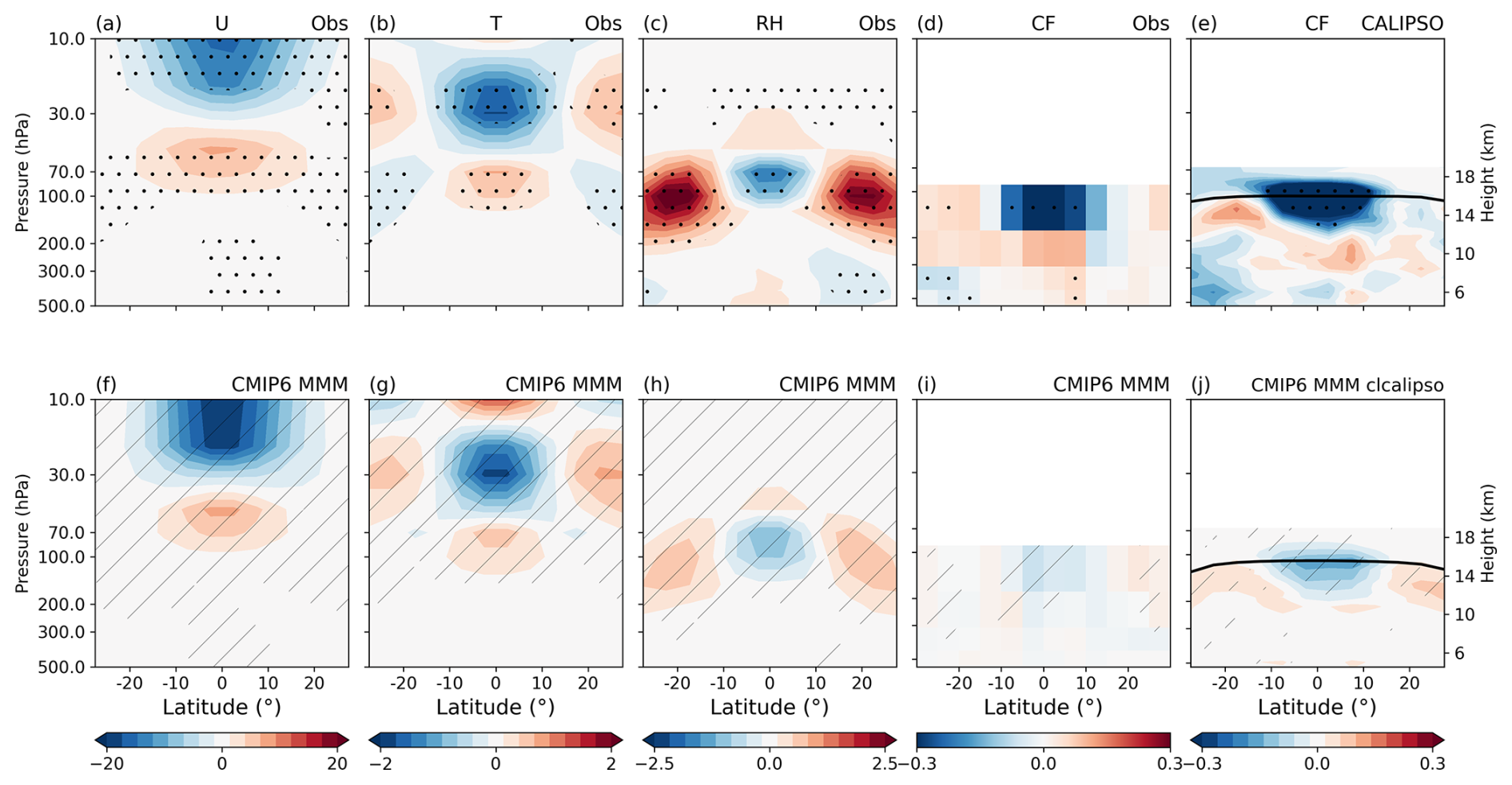
Figure 1 Latitude–height sections of QBO-regressed (a) zonal-mean zonal wind, (b) temperature, (c) relative humidity from ERA-5, (d) cloud fraction from MODIS and (e) CALIPSO between ±30° latitude. (f–j) Similarly for the CMIP6 multi-model mean, with (i) ISCCP-simulated cloud fraction and (j) CALIPSO-simulated cloud fraction. Panels are shown on pressure levels, except for panels (d) and (i), which use a bin-based representation defined by cloud top pressure, and for visualisation, the uppermost bin is limited to 90 hPa. Stippling marks statistically significant results in the top row (95 % confidence; 90 % for cloud fraction). Hatching denotes regions where six out of seven models agree on the sign. In panels (e) and (j), the black line denotes the mean tropopause pressure level.

The columns display the QBO-associated anomalies in temperature, relative humidity, zonal wind, and cloud fraction, respectively. The top row shows results from reanalysis and observations (Fig. 1a–e), while the bottom row presents the CMIP6 MMM (Fig. 1f–j). Consistent with the QBO index definition, westerly zonal wind anomalies are centred at 50 hPa (first column). In both observations (Fig. 1a) and the MMM (Fig. 1f), easterly anomalies dominate the mid–upper stratosphere (above 30 hPa) whereas westerly anomalies occupy the lower stratosphere, conforming to the QBO's well-known downward propagation over time. These positive zonal wind anomalies in the lower stratosphere descend to approximately 100 hPa, although the meridional extent is slightly broader in the observations than in the MMM.

When westerly (easterly) anomalies occupy the lower stratosphere, warming (cooling) is expected in the levels immediately below, driven by the QBO-induced meridional circulation. The resulting temperature anomalies can be linked to changes in moisture, with warming typically accompanied by reduced relative humidity. These expected QBO-related temperature and humidity anomalies are evident in Fig. 1 in both observations and the MMM. During the westerly phase, positive temperature anomalies extend from ∼ 70 hPa to below 100 hPa (Fig. 1b, g). Consistent with this warming, upper-tropospheric drying appears in the relative humidity field, with negative anomalies spanning 10° S–10° N and extending below 100 hPa, particularly in the MMM (Fig. 1c, h). However, QBO-associated temperature and relative humidity anomalies are weaker in the MMM compared to ERA-5.

Consistent with the QBO-associated warming and drying in the UTLS during the westerly phase, both observations and the MMM show a robust reduction in cloud fraction over the deep tropics (10° S–10° N). The QBO accounts for approximately 25 % of the variance in tropical-mean cloud anomalies in the 14–17 km layer, with the easterly phase associated with enhanced cloud fraction (Fig. S4).

The cloud fraction response to QBO in observations is analysed using MODIS and CALIPSO datasets (Fig. 1d and e), with a corresponding CMIP6 MMM analysis using ISCCP-simulated and CALIPSO-simulated CMIP6 model cloud fractions (Fig. 1i and j). While for MODIS (Fig. 1d) and ISCCP-simulated CMIP6 data (Fig. 1i), the cloud fraction is represented as a function of cloud top pressure, CALIPSO (Fig. 1e) and CALIPSO-simulated CMIP6 (Fig. 1j) cloud fraction represents vertically resolved profiles.

The reduction in cloud fraction in the deep tropics extends from 100 to 200 hPa in CALIPSO (Fig. 1e). A similar vertical structure appears in both MODIS observations and the MMM (Fig. 1d, e, i, j), although the vertical extent of the significant QBO-modulated cloud fraction anomalies is not obvious in these datasets due to their limited cloud top-pressure bins. Observations also suggest a weak and largely insignificant increase in cloudiness below 200 hPa. It is evident that CALIPSO exhibits a stronger QBO–high-cloud signal than MODIS, likely because its active lidar sensor better resolves the vertical profile of thin cirrus clouds in the upper-troposphere.

For CMIP6 models, the MMM very well captures the overall reduction in tropical zonal-mean high-cloud fraction in the deep tropics above 200 hPa, despite underestimating its magnitude. However, the magnitude and vertical extent of the response vary substantially across individual models, with some simulating cloud fraction anomalies extending down to 500 hPa (Figs. S5 and S6). For a clearer comparison between the observations and the MMM, a difference plot in the Supplement (Fig. S7) shows the observed minus MMM QBO regressed variables. The same colour-bar range is used for consistency and to highlight the regions where the model response differs most from observations.

As both observations and models indicate a clear QBO modulation of high clouds, we now examine the latitude-longitude profile of the QBO–high-cloud fraction relation. High-cloud fraction is defined as the cloud fraction at pressure levels lower than 440 hPa (above 6 km), consistent with the ISCCP definition and previous studies (Wilson Kemsley et al., 2025). For CALIPSO observation and MMM, which provide vertically resolved cloud fraction, Fig. 2 shows the mean cloud fraction within the selected layers. For MODIS and ISCCP (Fig. S8), which are binned by cloud-top pressure, the cloud fraction is summed across the corresponding pressure layers. Although Fig. 1 shows a clear vertical structure in the QBO–cloud relationship, we initially analyse the zonal structure of the total high-cloud fraction. This is because previous studies on the QBO–troposphere relationship have mostly focused on variables such as precipitation and outgoing longwave radiation, which may be reflected in the total high-cloud fraction (Collimore et al., 2003; Gray et al., 2018).

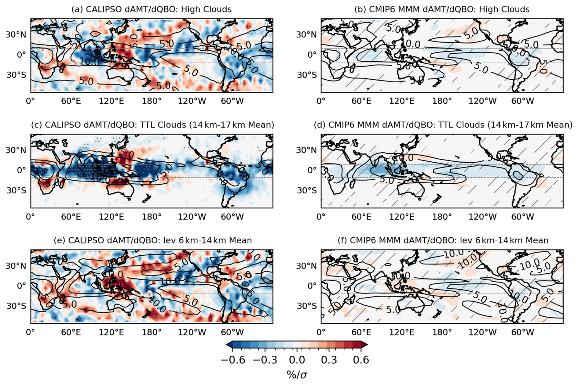
Figure 2 QBO regressed high-cloud fraction (< 440 hPa), TTL cloud fraction (< 180 hPa), and 440–180 hPa cloud fraction in CALIPSO (a, c, e) and CMIP6 MMM (b, d, f), represented in units of standard deviation of the QBO index. Overlaid line contours indicate the climatology of respective cloud fraction. Stippling in (a), (c) and (e) denotes 90 % confidence, and hatching in (b), (d) and (f) denotes six out of 7 models having the same sign.

Although the zonal-mean high-cloud fraction shows a robust reduction during a westerly QBO anomaly, the QBO influence on high clouds and convection is not zonally symmetric (Fig. 2). Figure 2a presents the tropical distribution of QBO-regressed high-cloud fraction anomalies in observations. Consistent with Fig. 1e, the reduction in cloud fraction is most pronounced in the deep tropics from 10° S to 10° N. Across this latitude band, particularly over the oceans, cloud reductions dominate, while over the African continent, a narrow band near the Maritime Continent, and regions west of South America, localized increases in cloud fraction are evident in association with anomalous westerly QBO winds. This spatial pattern strongly resembles results from previous regression or composite analyses of the QBO influence on outgoing longwave radiation, convective precipitation and high cloud fraction (Chen and Thompson, 2026; Collimore et al., 2003; Gray et al., 2018). Collimore et al. (2003) showed that QBO-related cloud reductions are most pronounced over regions typically occupied by deep convection. As our analysis includes thin cirrus, as well as deep convective high clouds and extended anvil clouds, background convection patterns and moisture availability likely modulate the regional QBO response. Figure S8 confirms that the zonally resolved QBO–cloud relationship is similar in ISCCP and MODIS observations as well. CMIP6 MMM roughly reproduces the observed spatial structure with a reduced high-cloud fraction in association with a westerly QBO anomaly in the deep tropics, but with a much weaker amplitude (Fig. 2b). While the observational QBO–cloud regression coefficients extend to values as low as −3 % σ⁻¹, a narrower colour-bar range is used in Fig. 2 to better highlight the signals in the MMM.

As Fig. 1 indicated the strongest cloud amount reduction above 200 hPa, instead of considering the full high-cloud fraction, we further separate the cloud fraction from 14 to 17 km near the tropical tropopause layer (TTL; Fig. 2c, d) from 440 to 180 hPa (6 to 14 km) cloud fraction (Fig. 2e, f). Different from the QBO–high-cloud regression profile, a more uniform reduction in TTL clouds (14 to 17 km) is evident across the deep tropics in both observations and the MMM. Overlaid contours indicate the climatology of TTL cloud fraction. In both observations and models, the climatology peaks over the Indian Ocean and the Maritime Continent, consistent with previous evidence that deep convection and TTL cloudiness peak over this region (Collimore et al., 2003; Lei et al., 2023; Son et al., 2017). In observations, the strongest QBO modulation of TTL clouds also occurs over the climatology peak in the Indian Ocean, Maritime Continent and West Pacific. While the MMM reproduces the peak over the Indian Ocean (although with much weaker magnitude), the response over the Pacific is more diffuse, with a significant response towards the Central Pacific. This is because most models agree on the relationship over Indian Ocean, while Pacific responses are spread between East and West Pacific (Fig. S9). To ensure that the longer time period available for CMIP6 models does not drive the differences between models and observations, the analysis is repeated using successive 20-year segments of each historical model simulation. Figure S9 highlights regions where the sign of the response is not consistent across the different 20-year periods. The figure confirms that, for most models, the prominent features are robust and agree across time windows.

Recent studies have highlighted a QBO–MJO relationship, with one of many proposed mechanisms involving the QBO modulation of clouds which could impact the radiative anomalies and hence the MJO, although uncertainties remain (Lin and Emanuel, 2023; Son et al., 2017; Trencham and Hood, 2024). Figure 2 indicates the strongest QBO-cloud relationship in observations occurs over the Maritime Continent where the MJO activity peaks, while models fail to capture this strength in cloud modulation. This could add to the models' failure to capture the proposed QBO-MJO relationship.

Figure 2e, f shows that, in observations, a westerly QBO anomaly results in an increase in cloud fraction in levels between 440 and 180 hPa, in most regions in the deep tropics such as over Africa, near the Maritime Continent, and the East Pacific. We note that there is little statistical significance to this relation. Unlike observations, the MMM has a much weaker response to QBO in these altitudes as well. The seasonality of the QBO–cloud relationship was examined, with results broadly consistent with Sweeney et al. (2023). The MMM exhibits biases in its seasonal response (see Sect. S2 and Fig. S2), whose causes are beyond the scope of the present study. Hereafter, we focus on the annual-mean cloud response to the QBO.

As the QBO–high cloud relationship is most prominent in the TTL, from 14 to 17 km, in the following part of this study, we focus on the mechanism for the QBO–TTL cloud relationship and what causes the difference between observations and the MMM.

3.2 CCF contributions to QBO–TTL-cloud relationship

We apply the CCF framework, described in Sect. 2, to reconstruct the spatial pattern of QBO-induced TTL-cloud anomalies shown in Fig. 2c and d. Figure 3a and h present the resulting reconstruction of QBO-regressed TTL-cloud fraction for observed and CMIP6 MMM respectively, computed using the CCF fields following Eq. (1). The reconstruction successfully captures the dominant spatial features of the QBO-TTL cloud relationship in both datasets. Sensitivity tests including alternative CCF combinations were also performed, such as surface temperature instead of upper troposphere temperature, and other upper tropospheric static stability indices. Figure S3 shows the reconstruction of QBO-regressed TTL cloud amount using different temperature and stability indices and confirms that the current CCF set outlined in the Data and Methods section provides the best agreement with the regression values. We note that alternative CCF sets may provide an improved reconstruction of QBO-cloud relationships. However, exploring other CCF sets is outside the scope of this study, and the reconstruction using the current CCF set performs well, with a spatial correlation of 0.87 to QBO-regressed TTL cloud amount (Fig. 3a compared to Fig. 2c).

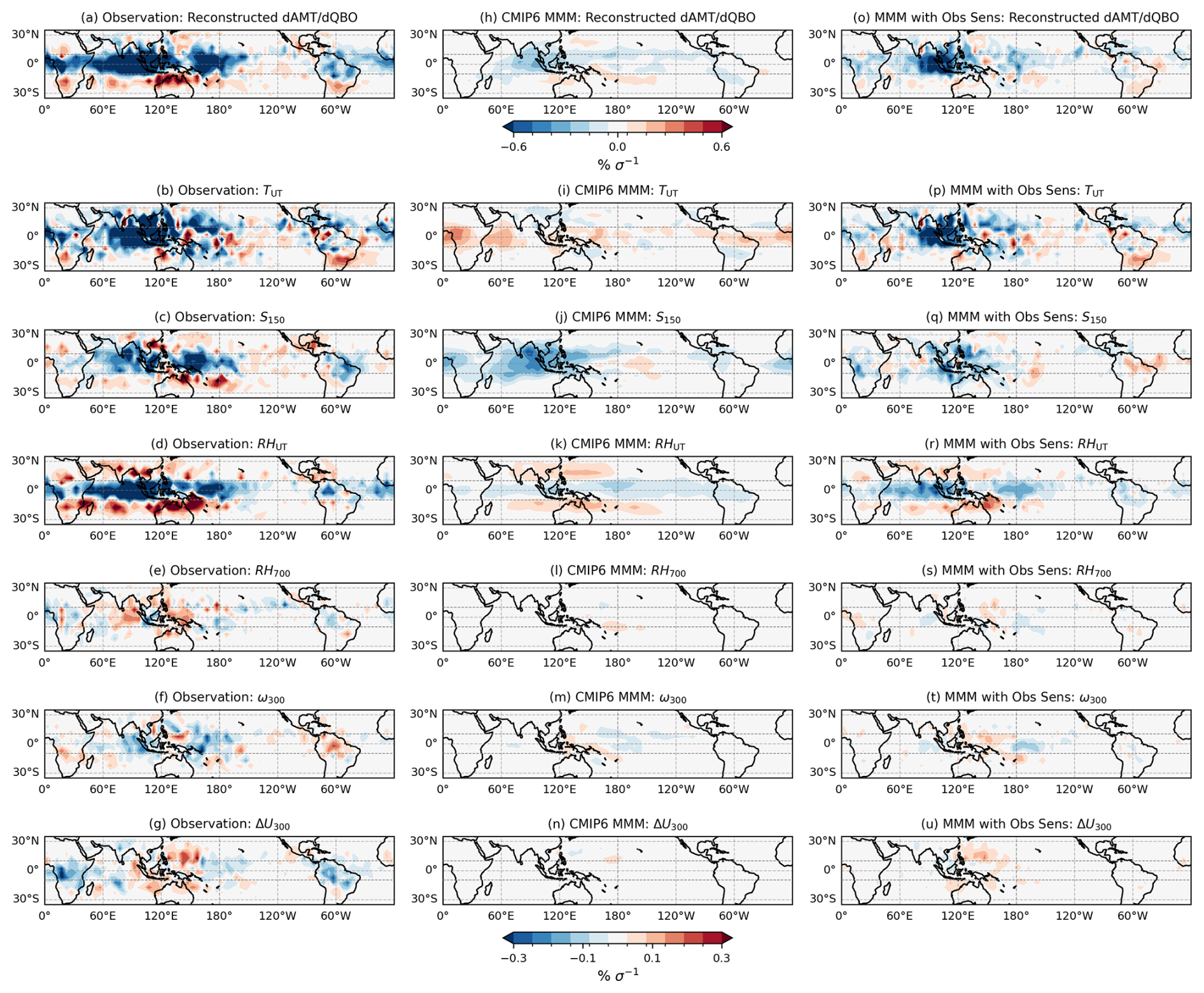
Figure 3 Reconstruction of QBO-regressed TTL cloud fraction anomalies using CCF analysis for (a) observations and (h) the CMIP6 MMM. (b–g) Contribution of each CCF to the observed QBO–TTL cloud relationship and (i–n) to the CMIP6 MMM QBO–TTL cloud relationship. (p–u) QBO-regressed CCFs from the CMIP6 MMM convolved with observed cloud sensitivities and (o) their sum.

The reconstruction captures the reduction of clouds over the Maritime Continent, stretching to the Indian Ocean and West Pacific in association with a westerly QBO anomaly with minor reductions over South America and the Atlantic in observations (Fig. 3a compared to Fig. 2c). The MMM reconstruction successfully captures the Indian Ocean cloud reduction and weaker reductions over the Pacific during a westerly QBO anomaly as seen in the MMM QBO-regressed TTL cloud fraction (Fig. 3h compared to Fig. 2d). Given the reasonable reconstruction using current CCFs in Fig. 3a, h, we use this framework to quantify the contribution of individual CCFs to the QBO–TTL cloud relationship.

Figure 3b–g shows the contribution of each CCF to the reconstruction of observed QBO-TTL cloud fraction relationship as shown in Fig. 3a. It is evident that the strongest drivers of the observed TTL cloud fraction reduction during QBO westerlies near the Indian Ocean and western Pacific are upper-tropospheric temperature, static stability at 150 hPa and upper-tropospheric relative humidity. While these CCFs can be correlated, since ridge regression learns separate sensitivities (Θ_i in Eq. 1), each CCF – local temperature (T_UT), static stability (S₁₅₀) and relative humidity (RH_UT) – makes an independent contribution to the QBO–TTL cloud relationship. To confirm this, Fig. S10 shows the CCF reconstruction of observed QBO-TTL cloud relationship using surface temperature (T_surface) instead of T_UT. The tropical-mean contribution of T_surface to the QBO–TTL cloud relationship is almost zero, while T_UT drives a strong reduction in clouds (Fig. 3b; see Fig. 5b for a direct comparison with Fig. S10), and swapping T_surface and T_UT had little impact on cloud sensitivities to other CCFs. This confirms that T_UT provides an independent contribution to the reconstruction, beyond its indirect influence through changes in static stability and relative humidity.

During QBO westerlies, warmer temperatures are present near the tropopause (Fig. 1b, g), which could increase the static stability and lead to upper tropospheric drying. Increased static stability suppresses convection, while reduced relative humidity indicates decreased moisture availability for cloud formation. In addition, warming may directly influence clouds through other pathways, such as via ice cloud micro-physics or cloud-top radiative cooling. Together, all three CCFs strongly contribute to the cloud fraction response to the QBO.

While T_UT, S₁₅₀ and RH_UT collectively drive the reduction in TTL cloud fraction associated with a westerly QBO anomaly in observations, these variables, despite being the dominant contributors, do not align spatially in the MMM (Fig. 3i–n). Although S₁₅₀ shows a considerable contribution over the Indian Ocean in the MMM, this is not supported by corresponding T_UT or RH_UT driven anomalies. Instead, the RH_UT mediated TTL cloud reduction peaks over the Central Pacific, while T_UT mostly contributes to increases in cloud fraction, and this misplaced response largely determines the spatial structure of the QBO-related TTL cloud-fraction anomalies in the MMM.

In both observations and the MMM, the remaining CCFs, RH₇₀₀, ω₃₀₀ and ▵U₃₀₀, contribute only marginally and exhibit zonally inhomogeneous signals. Although TTL clouds show strong sensitivities to these CCFs (Fig. S11c–e, i–k) – with, for example, enhanced cloud fraction with increased lower-tropospheric relative humidity or reduced cloud fraction during subsidence – the QBO induces only weak anomalies in these CCFs (Fig. S11cc–ee, ii–kk). As a result, their overall contribution to the QBO–TTL cloud relationship remains minimal. Thus, the QBO's impact on TTL clouds arises mainly from in-situ upper-tropospheric and lower-stratospheric variations rather than from surface-based processes.

To further understand why the T_UT, S₁₅₀ and RH_UT contributions to the QBO–TTL cloud relationship agree zonally in observations, but not in the MMM, we examine the contributions of (i) the sensitivity of cloud fraction to these CCFs (Θ_i on the RHS of Eq. 1) and (ii) the QBO-induced modulation of these CCFs themselves ($\mathrm{d}{\mathit{X}}_i\left(r\right)/\mathrm{dQBO}$ on the RHS of Eq. 1). Figure 3o–u shows the reconstructed QBO-driven TTL cloud anomalies generated using observational cloud sensitivities combined with QBO-modulated CCFs from the CMIP6 models. Figure 3o reveals stronger cloud modulation near the Maritime Continent, with the T_UT (Fig. 3p) and RH_UT (Fig. 3r) contributions closely matching the observed spatial patterns (Fig. 3b, d). This indicates that the MMM fails to reproduce the observed zonal structure of the QBO–TTL cloud relationship primarily because of biases in the spatial distribution of cloud sensitivities to CCFs, rather than biases in QBO signals. Note however that the QBO-modulated CCF anomalies in models are much weaker than in observations, especially for S₁₅₀ (Fig. 3q), leading to a weaker magnitude in the reconstruction.

Figure 4a–d shows the sensitivity of cloud fraction to S₁₅₀ and RH_UT in observations and the MMM, and Fig. 4e–h presents the corresponding QBO-driven CCF anomalies. Results for all CCFs, including T_UT, are shown in Fig. S11.

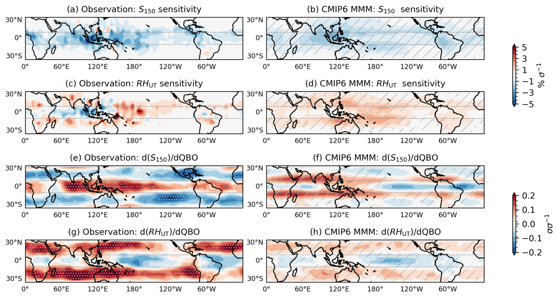
Figure 4 Historically derived sensitivities of the TTL cloud fraction to static stability at 150 hPa (S₁₅₀) and upper tropospheric relative humidity (RH_UT) in observations (a, c) and the CMIP6 MMM (b, d). QBO-regressed S₁₅₀ and RH_UT respectively, in units of standard deviation of CCF per standard deviation of QBO, in observations (e, g) and the CMIP6 MMM (f, h). Stippling in (e) and (g) marks statistically significant results (99 % confidence). Hatching in the right column denotes regions where six out of seven models agree on the sign.

Overall, the MMM captures the expected CCF–TTL cloud fraction relationships, that is, an increase in static stability reduces cloud fraction due to suppressed convection, and an increase in relative humidity enhances cloud fraction (but not over the Indian Ocean). However, the TTL cloud fraction sensitivity to S₁₅₀ and RH_UT peaks near the Maritime Continent and western Pacific in observations (Fig. 4a, c), and while models roughly reproduce this, the S₁₅₀ sensitivities fail to peak over the western Pacific, and RH_UT sensitivities are weaker in the deep tropics, especially over Indian Ocean (Fig. 4b, d).

In addition, the MMM fails to capture the observed static stability response to the QBO. Observations show a pronounced increase in static stability that peaks near the Indian Ocean, the Maritime Continent and the Western Pacific in association with a westerly QBO anomaly (Fig. 4e). Models do not reproduce this pattern and show a decrease in static stability throughout the deep tropics, except near the Maritime Continent (Fig. 4f). This discrepancy is likely linked to the well-known difficulty many models have in reproducing QBO signals at lower altitudes, which weakens their representation of associated UTLS stability changes. This can be confirmed from Fig. 1b and g, where QBO-induced temperature anomalies are weaker in the lower stratosphere in the MMM compared to ERA-5. Figure 1e and j also indicate that the models generally have a slightly lower tropopause than observed. This may contribute to small differences in the vertical profile of QBO influence on static stability between models and observations. The RH_UT response to the QBO is more consistent between models and observations, although observations show stronger drying in the West to Central Pacific and Atlantic (Fig. 4g), while models peak from Central to East Pacific (Fig. 4h).

Figure S11 (first row) presents TTL cloud sensitivity to T_UT and the QBO-modulated T_UT anomalies, using a different colour scale for easier comparison. The discrepancy between observations and the MMM, as expected from Fig. 3p, primarily stems from the small sensitivity values, where the observational pattern is more spatially irregular.

An important caveat when interpreting the sensitivities is that the maps shown in Figs. 4 and S11 represent a simplification of the underlying non-local relationships. As described in the methodology, to account for non-local influences, the sensitivity of cloud fraction to a given CCF at each grid box is calculated over a 21 × 11 grid-box domain. The resulting sensitivity is then summed across this domain and shown in Figs. 4 and S11. While this approach provides reasonable sensitivity profiles for S₁₅₀ and RH_UT, much of the signal associated with T_UT sensitivities is lost when summing across regional domains. Section S1 and Fig. S1 provide a detailed illustration of the T_UT sensitivities for a sample grid box. In observations, T_UT sensitivities are negative in the deep tropics over the Indian Ocean, indicating a decrease in cloud fraction with warming. In contrast, the CMIP6 MMM exhibits positive T_UT sensitivities, indicating an increase in cloud fraction with warming in the region. Thus, the discrepancy between observations and the MMM, as expected from Fig. 3p, primarily stems from the biased sensitivity values in the models.

The analysis indicates that in observations, T_UT, S₁₅₀ and RH_UT act together to reduce the TTL cloud fraction over the Indian Ocean and western Pacific, where deep convection and TTL cloud occurrence are climatologically strongest (Fig. 2c). In contrast, the MMM shows weaker or opposite TTL cloud sensitivities to T_UT, S₁₅₀ and RH_UT in this region, preventing the models from reproducing the observed spatial pattern. The exact reasons for the weaker or opposite TTL cloud sensitivities in the models remain unclear. Biases in the model mean state or an underestimation of mechanisms such as the stability-iris mechanism (Wilson Kemsley et al., 2025) could contribute to these discrepancies. Further, in observations, QBO-driven temperature anomalies and the associated changes in static stability can effectively modulate deep convection, thereby influencing convective TTL clouds over the Maritime Continent. However, in models, the absence of robust cloud sensitivities to temperature, along with incorrect static-stability responses to the QBO limits this pathway.

3.3 Inter-model spread

While we have focused on MMM changes so far, this section explores how individual models perform in the QBO–TTL cloud relationship and the causes for inter-model spread. Figure 5a shows the tropical-mean (10° S–10° N) QBO-regressed TTL cloud fraction. Observations indicate a reduction of approximately 0.54 % cloud fraction per standard deviation of the QBO index, while the CMIP6 mean reduction is around 0.12 %. Although all analysed models except HadGEM3 exhibit a reduction during QBO westerlies, the magnitude of the response varies substantially across models, with CNRM-ESM2-1 exhibiting the weakest reduction and MRI-ESM2-0 the strongest reduction.

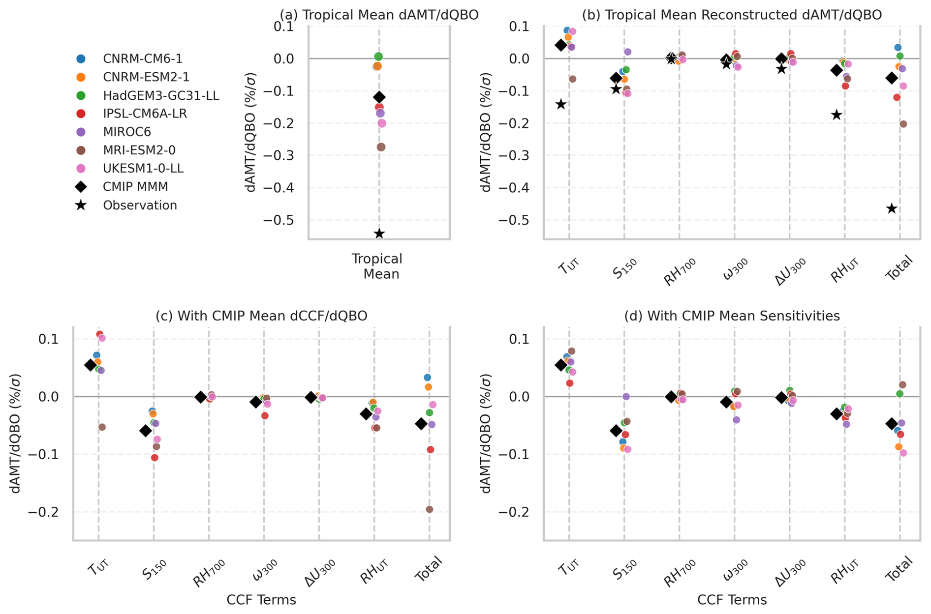
Figure 5 (a) Tropical mean (10° S–10° N) of QBO-regressed TTL cloud fraction in observations, CMIP6 models and the MMM. (b) Individual CCF contributions to the tropical-mean QBO-induced TTL cloud response and the total. (c) Same as (b) but replacing model-specific QBO-regressed CCF anomalies with the MMM CCF responses. (d) Same as (b) but replacing model-specific cloud sensitivities with the CMIP6 MMM sensitivities. Changes are per unit standard deviation of QBO.

Figure 5b presents the zonal-mean tropical-mean contribution of each CCF to the total reconstruction for observation and models. Total reconstruction and actual QBO-regressed cloud fraction are well correlated across models (0.87; Fig. S12). In observations, T_UT, RH_UT and S₁₅₀ provide the dominant contributions, as noted earlier. As seen in Fig. 3, the remaining CCFs had a weaker contribution, and were zonally irregular. Hence, these dynamically localized effects largely cancel in the zonal mean and therefore contribute less to the tropical-mean QBO signal.

Consistent with observations, climate models identify T_UT, RH_UT and S₁₅₀ as the strongest contributors towards the QBO–TTL cloud relationship. In all models, the RH_UT and S₁₅₀ terms play major roles in reducing TTL cloud fraction, although the RH_UT contribution is much weaker compared to observations (Fig. 5b). While T_UT plays an important role in observations to reduce cloud fraction, all models exhibit T_UT signals that differ from observations, with most of them suggesting an increase in cloud fraction under this pathway.

A key question of this study is what drives the inter-model spread in the QBO–TTL-cloud relationship: differences in how models simulate the QBO modulation of CCFs, or differences in cloud sensitivities to those CCFs. To address this, we reconstruct the tropical-mean QBO-induced cloud response (as in Fig. 5b) but systematically replacing (i) model-specific QBO-regressed CCF anomalies with the MMM CCF responses (Fig. 5c), and (ii) model-specific cloud sensitivities with the CMIP6 MMM sensitivities (Fig. 5d).

Comparison of the total terms in Fig. 5c and d indicates that both cloud sensitivities and QBO modulation play a part in the inter-model spread. In particular, the cloud sensitivities to T_UT and S₁₅₀ vary substantially across models (Fig. 5c), and this variability partly explains the spread in the simulated QBO–cloud relationships. An additional contribution comes from spread in the QBO modulation of T_UT and S₁₅₀, while QBO modulation of other CCFs is broadly consistent across models (Fig. 5d). A notable outlier is MRI-ESM2-0, which exhibits a strong negative sensitivity of TTL clouds to upper-tropospheric temperature. The pronounced reduction in TTL-cloud fraction in MRI-ESM2-0 is therefore driven primarily by its strong sensitivity of clouds to T_UT, distinguishing it from the other models.

Overall, Fig. 5 suggests that QBO-related tropical-mean TTL cloud variability is governed mainly by QBO-induced changes in RH_UT, T_UT and S₁₅₀, where the latter two also constitute the dominant source of inter-model spread.

4 Discussion and Conclusions

This study investigates the QBO–high cloud relationship using a CCF analysis approach applied to observations and CMIP6 climate models. While observations show that high cloud fraction in the deep tropics (10° S–10° N) decreases in association with a westerly QBO anomaly, we find that CMIP6 models with a reasonable QBO also capture this relationship in the zonal mean but systematically underestimate its amplitude. Furthermore, the zonal structure of the QBO–high cloud relationship is also misrepresented, and considerable inter-model differences exist, with better agreement over the Indian Ocean and larger differences over the Pacific. The high-cloud response to the QBO also exhibits strong vertical structure, with TTL clouds (14 to 17 km) decreasing during QBO westerlies while immediate lower-level (180–440 hPa; 6–14 km) cloud amounts show a modest increase.

We were able to reproduce the observed tropical pattern of the QBO–TTL cloud relationship using CCF analysis, with reduced cloud fraction associated with a westerly QBO anomaly across the deep tropics, dominated by changes over the Indian Ocean and western Pacific. We found that among the analysed CCFs, the largest contribution to the QBO–TTL cloud relationship is mediated by upper-tropospheric relative humidity, upper-tropospheric temperature and static stability at 150 hPa. Observed relationships support the theory that warmer temperatures, increases in stability and suppressed convection, and upper-tropospheric drying over deep convective regions during QBO westerlies jointly drive a reduction in cloud amount.

With a successful statistical reconstruction of the QBO–TTL cloud relationship in the models, we note that, although RH_UT, T_UT, and S₁₅₀ remain the dominant contributors to the cloud response, consistent with observations, these contributions do not align spatially, which is primarily due to biases in the spatial distribution of cloud sensitivities in the models. The models also underestimate the QBO-induced anomalies in these CCFs, especially in S₁₅₀. This could be due to the known issue of QBO signals not propagating to sufficiently low altitudes in models. Models also exhibit considerable spread in the QBO modulation of T_UT and S₁₅₀, and the TTL cloud sensitivities to T_UT and S₁₅₀, leading to substantial inter-model spread in QBO-TTL cloud relationship.

Comparison with previous studies provides useful context for interpreting the results in this study. The observational QBO–TTL cloud relationships presented here agree well with the findings of Sweeney et al. (2023), who used a different version of the CALIPSO dataset to understand the seasonality of the QBO–cloud relationship. Beyond reproducing the observed QBO–cloud relationship, our study examines how well climate models represent this relationship and investigates the underlying controlling factors. While this study focuses on the full analysis period, further CCF analysis of the seasonal variability would be valuable for understanding the mechanisms underlying the seasonal dependence of the QBO–cloud relationship identified by Sweeney et al. (2023).

Chen and Thompson (2026) recently used a linear regression-based methodology to understand the QBO–high cloud relationship arising due to static stability at 150 hPa. They found that S₁₅₀ plays an important role in the QBO modulation of high clouds over the Indian Ocean and Western Pacific region. While Chen and Thompson (2026) argue that the static stability effect of the QBO is physical and the remaining signals in the QBO–high cloud total regression relationship are relatively noisy, our results imply that S₁₅₀ alone does not fully explain the significant signals in the QBO–TTL cloud relationship. By expanding the set of controlling factors within the ridge regression framework, we are able to account for a larger fraction of the total QBO–TTL cloud linkage. In particular, upper-tropospheric temperature and relative humidity emerge as additional important controlling factors in the Indian Ocean and Western Pacific domain. This suggests that additional pathways may exist through which the QBO modulates TTL clouds, such as direct thermodynamic effects, including influences on ice-cloud microphysics (Tseng and Fu, 2017). Further investigation is required to identify such mechanisms.

While the inability of climate models to reproduce QBO signals in the lower stratosphere is often suggested as the possible reason for biases in QBO–troposphere relationships, our study highlights that biases in TTL cloud sensitivities to meteorological factors in the models is also an equally important, if not dominant, contributor. This is consistent with the results of Martin et al. (2021), who showed that models remained unable to capture the observed QBO–MJO relationship even with the stratosphere nudged to reanalysis fields. This suggests that other factors, such as grid resolution or convection and cloud parametrisations, may be responsible.

This study therefore highlights that, for models to accurately reproduce the observed QBO–TTL cloud relationship, a priority is to better represent TTL cloud sensitivities to the CCFs (and the underlying physical processes), and furthermore the QBO modulation of these CCFs needs to be stronger. While CALIPSO-GOCCP observations have limitations, and additional meteorological factors than those considered here may contribute to the QBO–cloud link, the present analysis provides a foundation for investigating how high clouds respond to a stratospheric forcing. We propose that this offers a useful framework for future analyses of the cloud response to climate change, including the contribution of greenhouse gas-driven stratospheric cooling to the cloud changes.