Physics-constrained transfer learning with a spectral-fidelity-preserving model for satellite remote sensing applications

Accurate spectral transformation across satellite sensors with similar but different spectral response functions (SRFs) is essential for applying the same retrieval algorithms. A novel physics-constrained transfer learning (TL) framework is developed for transferring satellite radiance observations across different sensors while preserving physical consistency. It integrates a core Spectral-Fidelity-Preserving (SFP) model based on extensive radiative transfer simulations, allowing broad adaptability for radiance transformation under diverse satellite observational conditions. Sensitivity experiments demonstrate the robustness of the TL framework relating to radiometric calibration uncertainties, particularly in infrared (IR) channels, and further highlight the critical role of SRF similarity between sensors. We further establish practical SRF-similarity thresholds – an allowable scaling-factor range and central-wavenumber-shift limits that are stricter for IR window channels – that support reliable radiance transfer (see Sect. 3.2 for details). Application to radiance observations from Fengyun-4A/B (FY-4A/B) geostationary (GEO) satellites explicitly indicates that the TL approach improves retrieval accuracy for key geophysical parameters such as cloud amount profile and quantitative precipitation estimation, when compared with results obtained without applying TL. Thus, the TL approach enhances cross-satellite data consistency and provides a practical tool for operational satellite data applications (e.g., transferring algorithms developed for FY-4A to FY-4B without operational interruption). It is worth noting that the FY-4A/FY-4B experiments presented here demonstrate retrieval-model transfer, validated against independent downstream satellite products. Beyond retrieval-model transfer, the framework can also support direct radiometric calibration transfer by propagating an absolute calibration reference at the radiance level between different spaceborne imagers.

1 Introduction

For operational continuity, machine learning (ML) enables rapid spectral transformation between similar spaceborne sensors with slightly different response functions, allowing algorithms trained on one sensor to be applied seamlessly to another without interruption. The history of transfer learning (TL) with ML dates back to the 1990s (Caruana, 1997), which was introduced to reuse knowledge across tasks or domains when labeled data or training resources are limited. After 2006, with the rise of artificial intelligence (AI), TL entered a new era of rapid development (Hinton et al., 2006; LeCun et al., 2015). Current TL techniques can be broadly categorized into five types: fine-tuning-based transfer learning (FTL), multi-task learning, few-shot learning, unsupervised domain adaptation (UDA), and self-supervised learning (SSL) (Ma et al., 2024). Each approach has emerged in response to rapid technological advances and evolving application scenarios. For example, the emergence of pre-trained models (e.g., ImageNet) (Krizhevsky et al., 2012) particularly enabled models to adapt to various downstream tasks through fine-tuning, establishing it as a core paradigm in modern TL (Pan and Yang, 2010). Besides, in recent years, large language models (LLM, e.g., the GPT (Generative Pre-trained Transformer) series) have further advanced the widespread application of TL, enabling cross-domain knowledge transfer from image processing to natural language processing (Jablonka et al., 2024; Joseph et al., 2024). Notably, the applications of TL in remote sensing have also grown explosively since 2017, including land-cover mapping, soil property estimation, vegetation monitoring, natural disaster management, etc. (Ma et al., 2024).

In remote sensing, TL is most widely applied to land-cover mapping and vegetation monitoring, accounting for approximately 48 % and 17 % of reported applications, respectively (Ma et al., 2024; Li et al., 2025). In land-cover mapping, models are commonly trained on high-accuracy, high-resolution land-cover reference data or obtained by fine-tuning pre-trained networks and are then transferred to otherunmanned aerial vehicle (UAV) or satellite imagery for broader application. For example, Nowakowski et al. (2021) similarly fine-tuned VGG-16 (Visual Geometry Group 16-layer network) and GoogLeNet on high-resolution imagery for crop mapping in Africa, achieving accuracies of approximately 83 %–90 % (Nowakowski et al., 2021). More recently, Zermatten et al. (2025) propose an open-vocabulary land-cover segmentation model that aligns pixel-level visual features with language embeddings using a pre-trained text encoder and a text augmentation strategy, enabling more flexible transfer across land-cover datasets with different label sets (Zermatten et al., 2025). The key concept of method is similar to that used in land-cover mapping, but vegetation monitoring primarily focuses on vegetation health, biomass estimation, and productivity. For instance, Bhadra et al. (2024) proposed a TL dual-stream neural network of PROSAIL-Net that leverages prior knowledge from numerical simulations to improve estimates of corn leaf chlorophyll concentration and average leaf angle under limited ground-truth data (Bhadra et al., 2024). Zhou et al. (2023) presented a deep TL framework that pretrains a Bi-LSTM (Long Short-Term Memory) model on MODIS (Moderate Resolution Imaging Spectroradiometer) reflectance and LAI (leaf area index) to learn temporally informed reflectance–LAI relationships, and then applies the transferred model to generate long-term Landsat LAI maps, outperforming traditional retrieval methods in both accuracy and robustness (Zhou et al., 2023).

With the exception of land-cover mapping and vegetation monitoring, natural disaster management ranks as the third most prevalent remote sensing application of TL (Ma et al., 2024), accounting for approximately 14 % of studies. In this domain, low-resolution meteorological satellite observations (Xia et al., 2024; Zhou et al., 2024a) consistently leverage knowledge from historical disaster or weather records to facilitate faster and more effective response mechanisms. Generally, dominant TL applications of meteorological satellites remote sensing primarily follow a self-supervised learning or unsupervised domain adaptation paradigm, often combined with fine-tuning-based TL. For example, several studies have applied data-driven TL by fine-tuning ImageNet-pre-trained models or multi-task feature TL to improve tropical cyclone (TC) center localization using geostationary satellite measurements (Zhou et al., 2024b; Wang and Li, 2023; Lee et al., 2025). For sparsely observed regions such as the Tibetan Plateau, a TL framework (UDA mode) combining deep neural networks (DNNs) and a U-Net (U-shaped convolutional network) was developed to improve MODIS-based estimates of near-surface air temperature, achieving strong agreement with independent stations (R² (coefficient of determination) = 0.92, RMSE (root-mean-square error) = 2.29 °C) and reducing RMSE by at least 7 % overall (Wang et al., 2025). Similar TL-based U-Net models have been developed and applied to Himawari-8 geostationary (GEO) satellite observations, substantially enhancing the retrieval accuracy of cloud-top height, cloud optical thickness, and cloud effective radius (Li et al., 2023). As another example of combination of FTL and SSL modes, Mateo-García et al. (2020) developed a deep learning model for cloud masking using Landsat-8 imagery and then transferred it for PROBA-V data using spectrally similar channels (Mateo-García et al., 2020). Besides, Wang et al. (2021) also pre-trained a precipitation retrieval model using the U.S. Geostationary Operational Environmental Satellite (GOES) data and then transferred it to generate China Fengyun (FY) GEO meteorological satellite precipitation dataset (Wang et al., 2021).

As discussed above, AI-based application models for meteorological satellites (Min et al., 2020; Wang et al., 2024; Kühnlein et al., 2014b; Li et al., 2024) are typically trained on data from a specific time window, often in a SSL mode (e.g., using a full year of data from 2025), and then generalized to subsequent periods (e.g., deployed from 2026 onward).These models have been widely used for a range of retrieval tasks, including cloud, aerosol, precipitation, wind, and convective system (Ma et al., 2021; Miller et al., 2024; McGovern et al., 2023; Min et al., 2019, 2020; Fu et al., 2024). Particularly in applications like tropical cyclone monitoring (Zhang et al., 2024), where building a long-term labeled training dataset is particularly slow, TL is crucial to maintaining operational continuity and performance consistency. However, in practice, temporal generalization and applicability of TL are frequently coupled with cross-sensor adaptation, where a pre-trained model is transferred to similar satellite instruments through a combination of UDA and FTL.

Accordingly, transfer learning in these AI-based remote sensing models still faces two major challenges: (1) within-series transfer, where models trained on earlier sensors' data must be migrated to newer satellites in the same series (e.g., transferring a model from China FY-4A to the newly launched FY-4B/C satellites); and (2) cross-platform transfer, where algorithms developed for one satellite sensor must be adapted to comparable sensors on other satellite systems (e.g., transferring approaches developed for the U.S. MODIS sensor to similar sensor onboard China Fengyun meteorological satellites). Hence, without an effective TL model, algorithmic consistency and retrieval quality can be severely compromised, which could interrupt operational applications of satellite observations from sensors onboard the same series or different platforms.

It turns out that, Bayes theorem has explicitly indicated that the label marginal distributions differ between the source (subscript: 0) and target (subscript: 1) domains, i.e., P₀(X) ≠ P₁(X), which in turn leads to slight differences in the conditional distributions P₀(X|Y) ≈ P₁(X|Y) (Ma et al., 2024). In other words, this represents a typical prior shift, where the observation variables (e.g., reflectance (Ref) or brightness temperature (BT) observed by satellite imager) used to pre-train an application model on the source satellite may differ from those available from the target satellite for transfer learning (Fig. 1). Figure 1 shows the different radiative signatures of cloud and ocean targets observed by nominally similar channels across satellites, which may degrade TL performance. According to physical theory, differences in P(X∣Y) across satellite observation periods are primarily caused by time-varying changes in an instrument measurement and calibration performance (Min et al., 2022; Doelling et al., 2013). In cross-satellite-instrument settings, however, beyond calibration effects, disparities in spectral response characteristics are the most critical driver of such shifts in P(X ∣ Y).

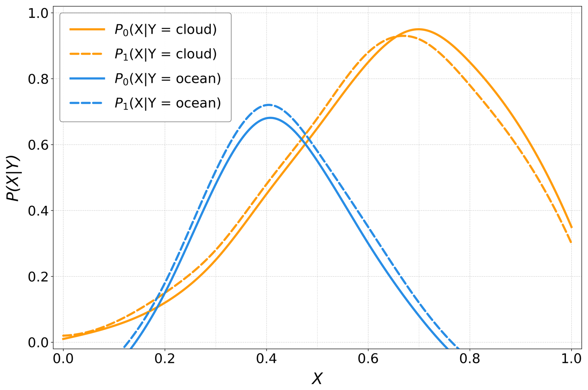
Figure 1 Prior shift in the conditional distributions P(X∣Y) of satellite-observed reflectance (Ref) or brightness temperature (BT) for assumed cloud (orange) and ocean (blue) targets. This shift (with subscripts 0 (solid line) and 1 (dashed line)) can occur when data are collected either by different satellite sensors or by the same sensor but over different time periods (Example inspired by Ma et al., 2024).

In addition, Fig. 2 compares the typical spectral response functions (SRFs) from the visible (VIS) to infrared (IR) channels across China FY-4A/B GEO imagers, the U.S. GOES-16 GEO imager, China FY-3D polar-orbiting imager, and the U.S. Aqua/MODIS (Yang et al., 2017; Platnick et al., 2017; Schmit et al., 2017). As shown in Fig. 2, differences in SRFs across satellites lead to substantial discrepancies in how nominally similar VIS and IR channels respond to atmospheric absorption and scattering effects (Min et al., 2017a; Hocking et al., 2021; Pearlman et al., 2013; Wang et al., 2024). Particularly, it shows that the SRFs at 0.86 and 2.25 µm channels on these satellite imagers differ in both spectral coverage and shape. Besides, FY-3D/MERSI-II SRFs are roughly 1.5 times wider than those of the corresponding MODIS bands, particularly for the longwave IR channels at 11 and 12 µm. These SRF discrepancies imply that TL for meteorological satellite applications can be highly sensitive to those discrepancies, potentially inducing observation biases (i.e., shifts in P(X∣Y) as illustrated in Fig. 1) and retrieval errors that are difficult to quantify.

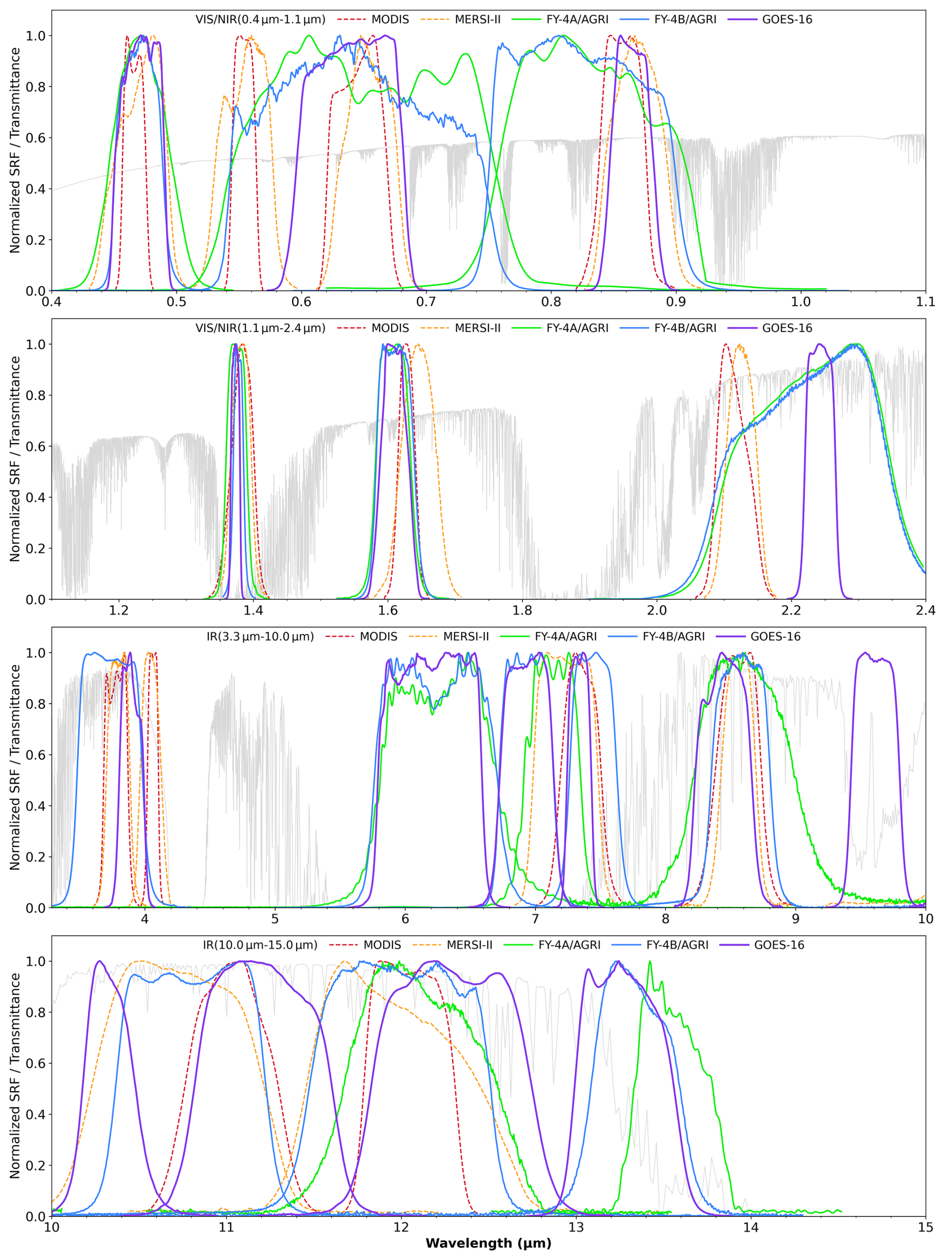
Figure 2 Normalized Spectral response functions from the visible to infrared channels across China FY-4A/B GEO imagers (AGRI, Advanced Geosynchronous Radiation Imager, green/blue solid line), the U.S. GOES-16 GEO imager (Advanced Baseline Imager, ABI, purple solid line), China FY-3D polar-orbiting imager (MERSI-II, Medium Resolution Spectral Imager II, orange dashed line), and the U.S. Aqua/MODIS polar-orbiting sensor (cardinal red dashed line). The light gray solid curve in each subfigure denotes the simulated transmittance using the 1976 U.S. Standard Atmosphere profile.

Therefore, it is essential to enable the reliable transfer of observed radiance across similar satellite channels, facilitating the inheritance of generalized retrieval algorithms for scientific products (Wang et al., 2021; Liu et al., 2024), and the propagation of radiometric calibration reference (Yu et al., 2026). For such purpose, a physics-constrained TL framework is developed for satellite remote sensing applications, which bridges the physical measurement (radiance) discrepancies between nominally similar channels across different satellite imaging sensors. Specifically, the core Spectral-Fidelity-Preserving (SFP) model, built on the radiative transfer simulations is developed, its accuracy and robustness are evaluated through numerical sensitivity analyses and retrieval experiments using real satellite SRFs and observations. Theoretically, this new TL framework for satellite remote sensing is grounded in classical atmospheric radiative transfer theories and calculations, thus differs from the conventional machine-learning-based approaches (Ma et al., 2024; Li et al., 2025). Superior transferability and generalization capabilities of the new TL model are achieved by offering stronger physical interpretability.

The remainder of this paper is structured as follows. Section 2 presents the proposed physics-constrained transfer learning framework. Section 3 examines the sensitivity of the core Spectral-Fidelity-Preserving model to satellite spectral response functions and radiometric calibration performance across the visible to infrared channels. Section 4 demonstrates the application of this TL framework to satellite retrieval experiments, highlighting its positive impact on satellite-based applications. Section 5 concludes the paper with a summary of the main findings, along with a discussion of limitations and directions for future work.

2 Physics-constrained Transfer Learning Framework

This section introduces the construction of the core Spectral-Fidelity-Preserving model, along with the overall framework and workflow of the proposed physics-constrained TL approach. In the following sections, we use the primary observation channels of the Advanced Geosynchronous Radiation Imager (AGRI) onboard the FY-4A and FY-4B satellites (Min et al., 2017b) as a test case to evaluate the performance of the SFP model. Because the two instruments have different numbers of channels, we only select 14 matched channels spanning 0.47–13.5 µm for the analysis (Fig. 2). Note that the same physical channel may therefore be numbered differently under the two sensors' designations; for example, the ∼ 13.30 µm channel corresponds to Channel 14 under the FY-4A numbering and Channel 15 under the FY-4B numbering. Channel numbers cited in this manuscript follow the FY-4B designation unless otherwise noted.

2.1 Spectral-Fidelity-Preserving Model

Based on atmospheric radiative transfer theory, the satellite-observed top-of-atmosphere (TOA) monochromatic radiance L^TOA in the visible/near-infrared (VIS/NIR) and thermal infrared (TIR) channels can be expressed in the following simplified forms (Kotchenova et al., 2006):

$$\begin{array}{}\text{(1)}& {\displaystyle }{L}_{\mathrm{VIS}/\mathrm{NIR}}^{\mathrm{TOA}}=L_{\mathrm{scat}}{T}^{\uparrow }+{\displaystyle \frac{(\mathrm{1}-\mathit{ϵ})}{\mathit{\pi }}}{E}_{\mathrm{0}}{\mathit{\mu }}_{\mathrm{0}}{T}^{\downarrow }{T}^{\uparrow }\text{(2)}& {\displaystyle }{L}_{\mathrm{TIR}}^{\mathrm{TOA}}=\mathit{ϵ}B\left(T_{\mathrm{s}}\right)T^{\uparrow }+{\int }_{\mathrm{0}}^{\mathrm{\infty }}B\left(T\right(z\left)\right)W\left(z\right)\mathrm{d}z\end{array}$$

where L_scat denotes the combined contribution from both single and multiple scattering by particles (e.g., clouds and aerosols) as well as gas molecules. ϵ is the surface emissivity. E₀ and μ₀ represent the incoming solar irradiance and the cosine of the solar zenith angle, respectively. T with arrows indicates the atmospheric transmittance along the downward and upward paths. It is primarily controlled by the total extinction optical depth along the line of sight, which depends on gaseous absorption (e.g., H₂O, CO₂, O₃) and scattering by clouds and aerosols, as well as the atmospheric temperature–pressure structure and viewing geometry (path length/zenith angle). In Eq. (2), B is the Planck function, which is used to compute the emitted radiance associated with the surface temperature T_s. The integral term accounts for the radiance emitted from each atmospheric layer at altitude z, and W(z) is the corresponding weighting function. W(z) quantifies the relative contribution of emission from atmospheric layer (z) to the TOA radiance; it is essentially the product of the layer's absorptivity (or emissivity) and the transmittance from that layer to the sensor, thereby indicating the altitude range to which a given channel is most sensitive (Matricardi, 2010).

For the 3.75 µm channel, the daytime top-of-atmosphere radiance includes both thermal and solar contributions. The thermal part arises from atmospheric path emission and surface emission, whereas the solar part originates from atmospheric scattering and surface-reflected solar radiance. Consequently, neither Eq. (1) nor Eq. (2) alone can fully describe the daytime radiative behavior of this mixed channel. In the SFP framework, the radiative transfer for the 3.75 µm channel is therefore performed using the total band-integrated radiance, rather than a thermal-only component. At night, the solar contribution becomes negligible, and the channel behaves essentially as a purely thermal emissive band.

From the physical interpretation of the above two equations, the primary factors affecting satellite-observed radiance include the atmospheric thermodynamic structure (temperature and humidity profiles), satellite viewing geometry, surface reflective and emissive properties, and extinction by atmospheric gas composition, clouds, and aerosols. A key scientific challenge for the TL model is therefore to develop a generalizable framework that can accurately propagate these physical effects across satellites for spectrally similar channels. Because these channels are spectrally similar (e.g., the examples shown in Fig. 2), we aim to exploit their underlying physical relationships to enable robust transfer of spectral radiance features across satellite observations.

Building on the rationale outlined above, we develop a physics-constrained TL model using simulated, satellite-sensor-consistent high-resolution spectral radiances. Specifically, we employ the classical MODTRAN (Version 5.3.2) model (Berk et al., 2013) as the forward radiative transfer model (RTM) to generate TOA radiances (Unit = W (m² sr µm)⁻¹) over 0.40–13.5 µm at a spectral resolution of 1 cm⁻¹. For computational convenience, the simulations are conducted over two subranges: 0.3–2.4 µm (VIS and NIR) and 3.3–13.5 µm (TIR). To ensure diversity and global representativeness, we compile 83 representative atmospheric profiles from the European Centre for Medium-Range Weather Forecasts (ECMWF) archive spanning multiple climate regimes. In addition to the 83 independent atmospheric profiles, we further enhance the diversity of the simulations by specifying a comprehensive set of cloud, aerosol, surface, and viewing-geometry parameters, as summarized in Table 1. This shows that cloud optical depth at 550 nm ranges from 0 (clear sky) to 216 (cumulus), with other four different cloud types. Surface reflectivity (ρ) is prescribed by land-cover type, varying from 0.003–0.979 (snow) and 0.08–0.83 (forest) to 0.01–0.05 (ocean) and 0.019–0.137 (urban). The observation geometry is configured with a set of discrete angles, which together cover the major satellite observation modes. Overall, these configurations generated 55 600 VIS/NIR simulation cases and 18 000 IR simulation cases before validity screening. The resulting SFP dataset constitutes a large-scale database of simulated satellite hyperspectral radiances, primarily spanning two spectral ranges as noted above: 0.3–2.4 µm (VIS/NIR) and 3.3–13.5 µm (TIR).

Table 1 Input variables and the corresponding values for RTM simulations.

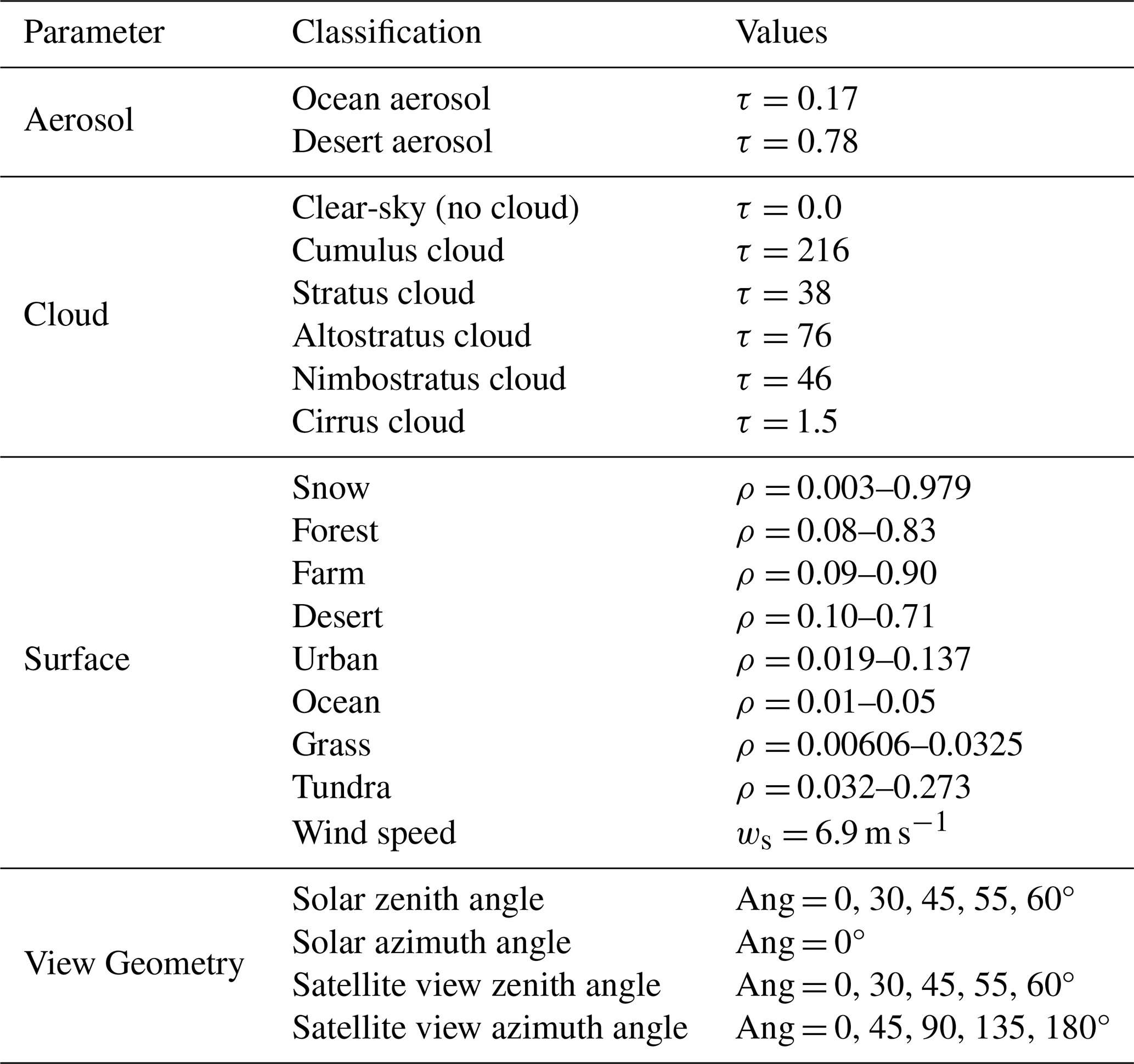
Note: τ= Optical depth at 550 nm. ρ= Reflectivity. Ang = Angle (degree). w_s = wind speed. The VIS/NIR simulations used solar zenith angles of 0, 30, 45, 55, and 60°, whereas the retained infrared simulation dataset used for the 3.75 µm Channel 07 analysis contained solar zenith angles of 0, 30, and 60°. Therefore, the angular assessment of Channel 07 was restricted to these three available discrete solar zenith angles.

For the 3.75 µm channel, the retained infrared simulations were generated using MODTRAN's thermal-plus-solar radiance mode (IEMSCT = 2), with multiple scattering enabled (IMULT = 1). The TOTAL_RAD output in tape7 includes atmospheric and surface thermal emission, atmospheric solar scattering, and ground-reflected solar radiance. This total radiance was subsequently used for the spectral response function (SRF) convolution. Consequently, the transfer coefficients for FY-4A and FY-4B Channel 07 were fitted using their respective SRF-convolved total radiances, rather than thermal-only components. Surface reflection was represented by the Lambertian assumption as configured in the MODTRAN input settings.

This SFP model was originally developed for the cross-calibration of the reflective solar bands of FY-3D/MERSI-II. By employing TL, it enables the transfer of the radiometric reference from the MODIS sensor while preserving the inherent radiometric observation characteristics of MERSI-II (Yu et al., 2026). Application of this model to the FY-3D/MERSI-II solar reflective channels over a period of more than seven years resulted in a mean relative bias of approximately 1 %, with a 2 %–3 % improvement compared with the operational calibration coefficients. We emphasize that, unlike physics-informed neural network approaches that enforce physical consistency through an explicit penalty term in the loss function, physical consistency in this framework is embedded directly in the construction of the training data: the fitting pairs used in Sect. 2.2 are derived from these MODTRAN radiative transfer simulations convolved with the actual sensor SRFs, so the resulting transfer coefficients are, by construction, consistent with radiative transfer physics. This is also the mechanism by which the framework reduces SRF-driven bias between sensors, since the fitting pairs already encode the true SRF discrepancy rather than requiring it to be inferred from noisy real satellite matchups.

2.2 Application of New Physics-constrained Transfer Learning Framework

Radiance TL between the target and reference instruments (using FY-4A and FY-4B AGRI as an example) is achieved through an adaptive polynomial framework. In this approach, transfer coefficients are derived by fitting the simulated radiances of both the reference and target sensors, with the theoretical radiances generated from MODTRAN simulations mentioned in section 2.1. The underlying polynomial model is expressed as follows:

$$\begin{array}{}\text{(3)}& y={\sum }_{i=\mathrm{0}}^n{a}_i{x}^i\end{array}$$

where y (i.e., the radiance observed by the target sensor) denotes the fitted value of the dependent variable corresponding to the input variable x (i.e., the radiance observed by the reference sensor), n is the polynomial order, a_i represents the polynomial coefficients to be estimated, and i is the index of the polynomial term.

The new physics-constrained TL framework uses a lowest-order-first adaptive polynomial fitting strategy. Fitting begins with a linear model (n=1), and the polynomial order is increased only when R²<0.95, up to a maximum of n=4. If the threshold is not reached at n=4, the model with the highest R² is retained. Here, R²≥0.95 is used as an empirical goodness-of-fit criterion rather than as a test of statistical significance, while limiting the polynomial order to four constrains unnecessary model complexity and reduces the risk of overfitting. For the VIS/NIR channels, a common finite-value mask was applied across the six matched channel pairs. Of the initial 55 600 simulated pairs, 50 cases containing non-finite values in at least one matched channel were excluded, leaving the same 55 550 pairs for each VIS/NIR channel fit. Each IR channel fit used 18 000 valid simulated pairs from five atmospheric conditions. Before fitting, the MODTRAN-simulated hyperspectral TOA radiances are convolved with the SRFs of the target and reference sensors to obtain the corresponding broadband channel radiances. The channel-averaged radiance $L_{\mathrm{Averaged}}^{\mathrm{TOA}}$ measured by a sensor channel is calculated by:

$$\begin{array}{}\text{(4)}& L_{\mathrm{Averaged}}^{\mathrm{TOA}}={\displaystyle \frac{{\int }_{{\mathit{\lambda }}_{\mathrm{2}}}^{{\mathit{\lambda }}_{\mathrm{1}}}{L}^{\mathrm{TOA}}\left(\mathit{\lambda }\right)\cdot \mathrm{SRF}\left(\mathit{\lambda }\right)\mathrm{d}\mathit{\lambda }}{{\int }_{{\mathit{\lambda }}_{\mathrm{2}}}^{{\mathit{\lambda }}_{\mathrm{1}}}\mathrm{SRF}\left(\mathit{\lambda }\right)\mathrm{d}\mathit{\lambda }}}\end{array}$$

where λ₁ and λ₂ denote the starting and ending wavelengths of the normalized spectral response function (SRF), respectively. Overall, Eqs. (3) and (4) are designed to provide physically consistently observed radiance for bridging the target and reference channels. Furthermore, for practical remote sensing applications, the observed radiances of the VIS/NIR channels and IR channels need to be converted into reflectance (ρ, Eq. 5) and brightness temperature (BT, Eq. 6), respectively, which are written as follows:

$$\begin{array}{}\text{(5)}& {\displaystyle }\mathit{\rho }={\displaystyle \frac{\mathit{\pi }{L}_{\mathrm{Averaged}}^{\mathrm{TOA}}}{\cos \left({\mathit{\theta }}_{\mathrm{0}}\right)F_{\mathrm{0}}}}\text{(6)}& {\displaystyle }\mathrm{BT}=\mathrm{Planck}(L_{\mathrm{Averaged}}^{\mathrm{TOA}},{\mathit{\lambda }}_{\mathrm{emw}})\end{array}$$

where θ₀ is the solar zenith angle, F₀ represents the channel SRF-convolved solar exo-atmospheric irradiance. Additionally, Planck denotes the Planck function, and λ_emw corresponds to the effective middle wavelength weighted by the channel SRF. Note that, the IR channels require additional correction because they are not ideal narrowband filters. As a result, a slight difference exists between the nominal central wavelength and the effective central wavelength used in BT calculations based on the Planck function (Chen et al., 2012). The fitting coefficients and Planck-weighted correction coefficients (for IR channels only) for the FY-4A/B AGRI channels used in this study are provided in Tables S1 and S2 in the Supplement.

Channel 07 is processed through the thermal-channel branch, as the operational FY-4A and FY-4B products provide it in brightness-temperature form. During daytime, this brightness temperature should be regarded as an effective brightness temperature corresponding to the total measured band radiance. In practice, the observed brightness temperature is first converted to radiance; the inter-sensor transfer is then performed in radiance space, and the transferred radiance is subsequently converted to the target-sensor brightness temperature. This procedure retains the mixed daytime signal but does not explicitly isolate or remove the solar-reflected component. Consequently, the brightness-temperature-based formulation represents the transfer of the total channel signal, rather than a purely thermal treatment of the 3.75 µm channel.

Figure 3 illustrates the TL models used to convert four representative FY-4B/AGRI channels (Channels 1 (0.47 µm), 5 (1.61 µm), 13 (10.80 µm), and 15 (13.30 µm)) to their corresponding FY-4A/AGRI channels within the new physics-constrained framework. This conversion spans VIS, NIR, and TIR spectral bands, and includes a case employing higher-order polynomial fitting. As shown in this figure, the fitting performance is excellent in the solar reflective bands, such as Channels 1 and 5, with only very small fitting residuals. In contrast, the longer-wavelength Channel 15 exhibits not only larger residuals but also a need for a quadratic term in the fitting. Besides the slight differences in the central wavelengths of this channel (see the bottom panel in Fig. 2), the larger errors in the TIR bands are primarily caused by the more complex gaseous absorption characteristics at these wavelengths, especially carbon dioxide (CO₂) absorption (Teixeira et al., 2024).

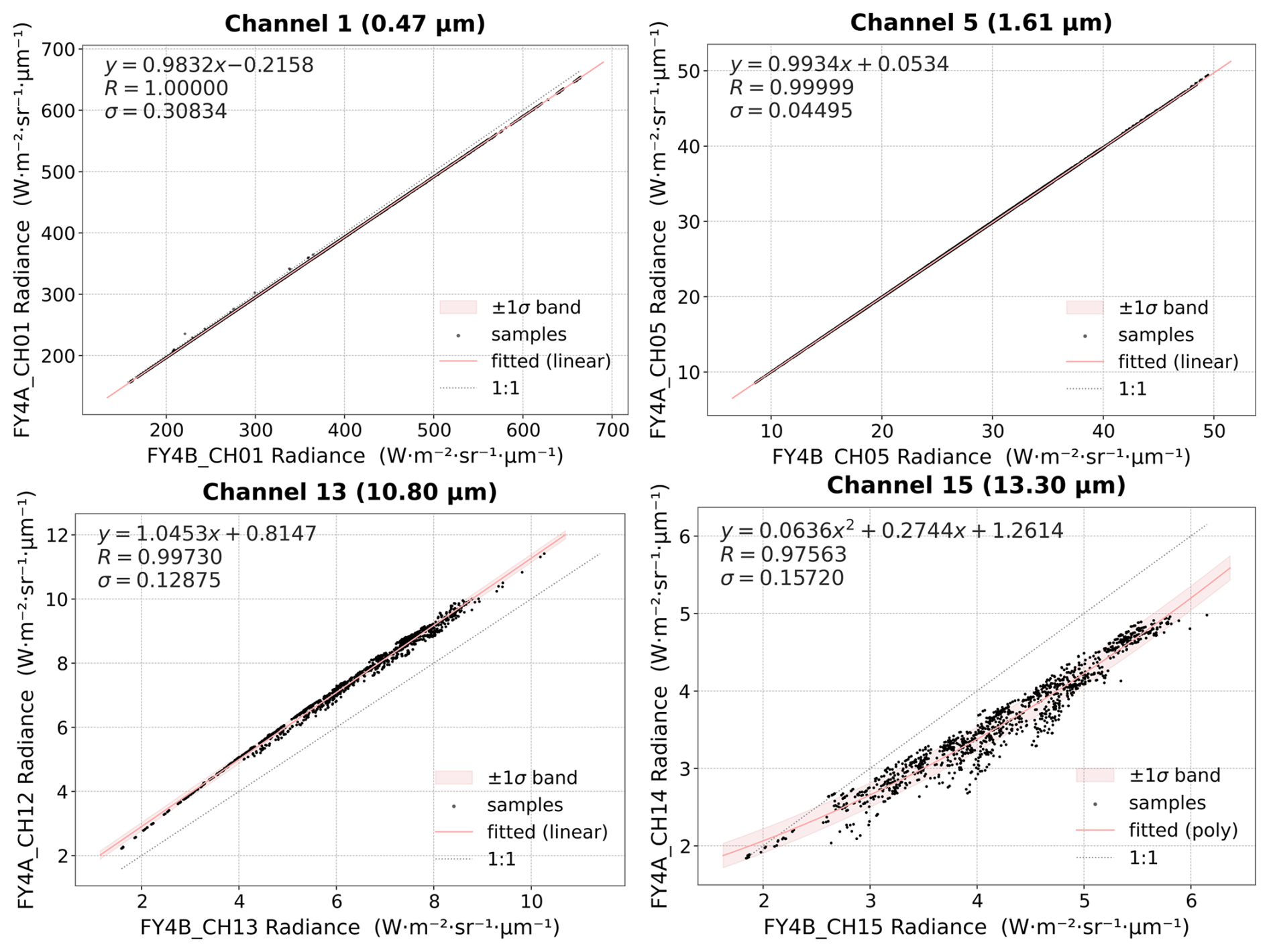
Figure 3 Application of the new physics-constrained transfer learning framework from FY-4B to FY-4A AGRI radiance observations. From left to right, the panels show Channels 1 (0.47 µm), 5 (1.61 µm), 13 (10.80 µm), and 15 (13.30 µm) (following the FY-4B channel designations). They demonstrate the framework's linear fitting performance in the visible, near-infrared, and thermal infrared bands, as well as an example of higher-order polynomial fitting for FY-4B/AGRI Channel 15 (13.30 µm). R and σ denote the correlation coefficient and fitting residuals, respectively.

Differences in central wavelengths or SRFs, combined with strong path absorption and emission, introduce substantial nonlinearities into the radiative transfer process. As a result, lower-order linear fitting becomes insufficient, and higher-order terms must be incorporated. Therefore, the next Sect. 3 investigates the sensitivity of the physics-constrained TL model to those discrepancies in the SRFs of satellite sensors and their radiometric calibration uncertainties, using the AGRIs aboard the FY-4A and FY-4B satellites as examples.

3 Transfer Learning Sensitivity to Changes in Spectral Response Functions and Calibration Status

3.1 Simulated SRFs and their Discrepancies

We simulate discrepancies in the SRFs of spaceborne imager by scaling the spectral width and shifting the central wavelength. The spectral width scaling factor ranges from 0.1 to 2.0 in increments of 0.1. The central wavelength is shifted from −100 cm⁻¹ (“−” means a leftward shift) to +100 cm⁻¹ (“+” means a rightward shift) in increments of 10 cm⁻¹ for IR channels. For VIS/NIR channels, due to the relatively large wavenumber, the central wavenumber is shifted from −1000 to +1000 cm⁻¹ in increments of 100 cm⁻¹. Figure 4 shows examples of these simulated (or adjusted) SRFs for FY-4B/AGRI Channel 2 (0.66 µm) and Channel 13 (10.80 µm), including cases with narrower and wider spectral widths as well as shifts in central wavelength. As shown in Fig. 4, the discrepancies between the adjusted SRFs and the original SRFs are still substantial. Whether excessively large SRF differences between the target and reference sensors may affect the performance of this new TL approach is a question that warrants careful evaluation and consideration.

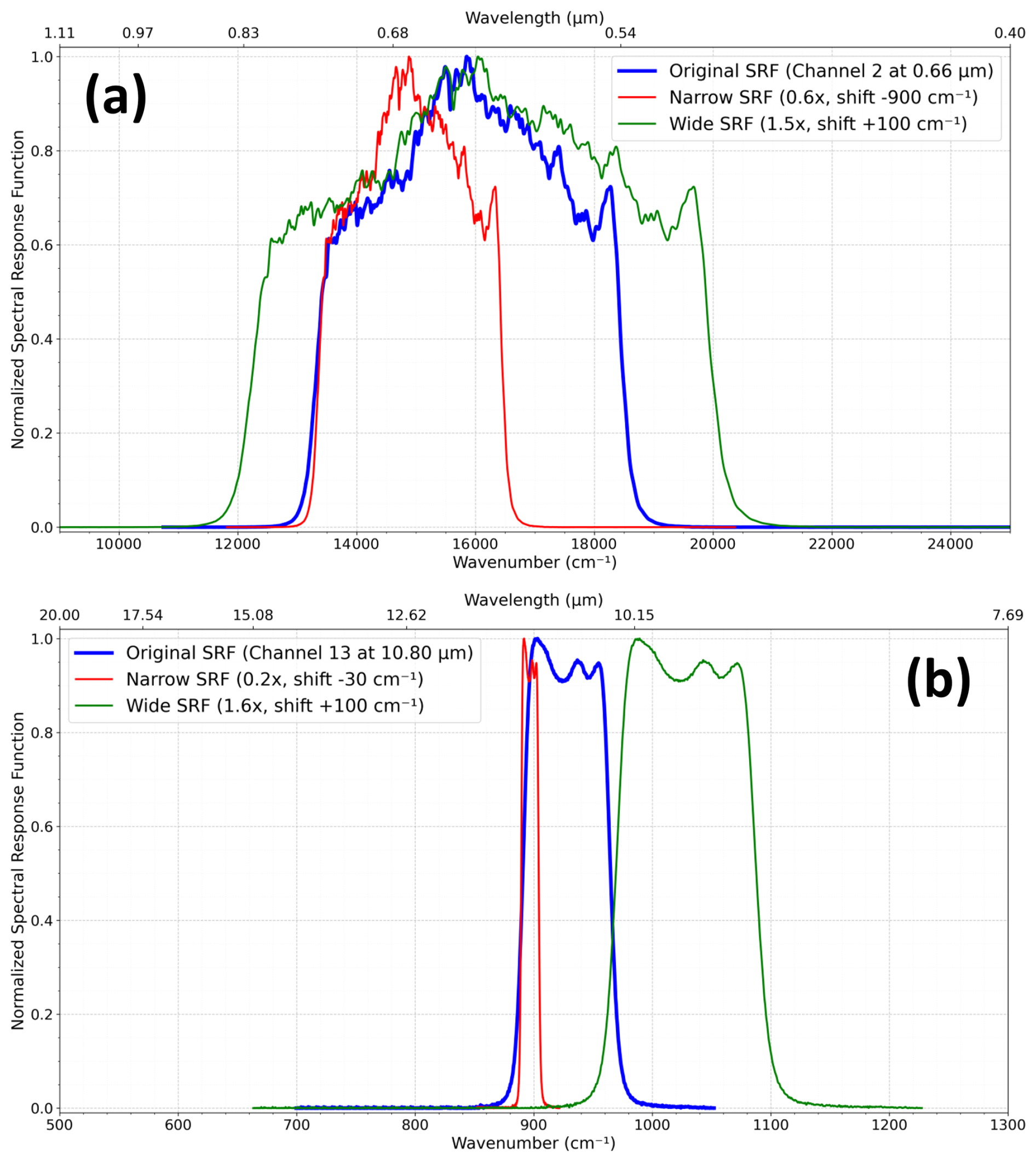
Figure 4 Original SRFs (blue solid lines) and two simulated SRFs, including a narrower SRF (red solid lines) and a wider SRF (green solid lines), for FY-4B/AGRI: (a) Channel 2 at 0.66 µm and (b) Channel 13 at 10.80 µm. Here, 0.2/0.6/1.5/1.6× indicates 0.2/0.6/1.5/1.6× (or scaling factor) the width of the original SRF, shift −30/−900 cm⁻¹ denotes a leftward shift of 30/900 cm⁻¹, and shift +100 cm⁻¹ denotes a rightward shift of 100 cm⁻¹.

In this investigation, we employ three classical metrics, namely Jensen–Shannon divergence (JSD), Wasserstein distance, and Kolmogorov–Smirnov distance (KS), to evaluate the similarity between the adjusted SRFs and the original SRFs. For the calculation of the Jensen–Shannon divergence (Endres and Schindelin, 2006), the two curves (or SRFs) are first discretized into histograms or grids and represented as probability distributions, which is defined as:

$$\begin{array}{}\text{(7)}& P=\left(p_{\mathrm{1}},p_{\mathrm{2}},\mathrm{\dots },p_n\right),Q=\left(q_{\mathrm{1}},q_{\mathrm{2}},\mathrm{\dots },q_n\right)\end{array}$$

where $\sum p_i=\sum q_i=\mathrm{1}$ and $M=\frac{\mathrm{1}}{\mathrm{2}}\left(P+Q\right)$. JSD is a symmetric and smoothed variant of the Kullback–Leibler divergence (KL), which is defined as follows:

$$\begin{array}{}\text{(8)}& {\displaystyle }\mathrm{JSD}\left(P\left|\right|Q\right)={\displaystyle \frac{\mathrm{1}}{\mathrm{2}}}\mathrm{KL}\left(P\left|\right|M\right)+{\displaystyle \frac{\mathrm{1}}{\mathrm{2}}}\mathrm{KL}\left(Q\left|\right|M\right)\text{(9)}& {\displaystyle }\mathrm{KL}\left(P\left|\right|M\right)={\sum }_i{p}_i\log \left({\displaystyle \frac{p_i}{m_i}}\right)\end{array}$$

The JSD is dimensionless and ranges from 0 to 1, with smaller values indicating greater similarity between the two curves.

The second metric is the Wasserstein distance (Mémoli, 2011), also referred to as the Earth Mover's Distance, which measures the minimum transportation cost required to transform one probability distribution into another. For one-dimensional distributions, the first-order Wasserstein distance can be expressed as:

$$\begin{array}{}\text{(10)}& W\left(P,Q\right)={\int }_{-\mathrm{\infty }}^{+\mathrm{\infty }}|F_P\left(x\right)-F_Q(x\left)\right|\mathrm{d}x\end{array}$$

where F_P(x) and F_Q(x) are the cumulative distribution functions (CDFs) of P and Q curves, respectively. This metric reflects not only distributional overlap but also the geometric displacement between them.

The third metric is the Kolmogorov–Smirnov distance (Massey, 1951), which is defined as the maximum absolute difference between the two CDFs and can be written as:

$$\begin{array}{}\text{(11)}& D_{\mathrm{KS}}={\sup }_x|F_P\left(x\right)-F_Q(x\left)\right|.\end{array}$$

It characterizes the largest pointwise discrepancy between two curve distributions. Together, these three metrics provide complementary perspectives on distributional differences: JSD emphasizes probabilistic similarity, Wasserstein distance captures transportation-based discrepancy, and KS measures the maximum deviation between cumulative distributions.

Figures 5 and 6 show the distributions of Jensen–Shannon divergence, Wasserstein distance, and Kolmogorov–Smirnov distance as functions of the scaling factor (from 0.1 to 2.0) for FY-4B/AGRI Channel 2 (0.66 µm, with shifted wavenumber from −1000 to +1000 cm⁻¹) and Channel 13 (10.80 µm, with shifted wavenumber from −100 to +100 cm⁻¹), respectively. From these two figures, the shortwave band, Channel 2 (0.66 µm), exhibits relatively low sensitivity to wavenumber shifts within ±1000 cm⁻¹ because of its comparatively broad spectral width (about 3000 cm⁻¹), whereas the narrower longwave band, Channel 13 (10.80 µm), is considerably more sensitive. However, when the wavenumber shift reaches more than 1000 cm⁻¹, even the shortwave band is likely to be affected significantly. Considering the limitation of the manuscript length and the similar distribution characteristics, the results of other FY-4B/AGRI channels are presented in Figs. S1 to S13.

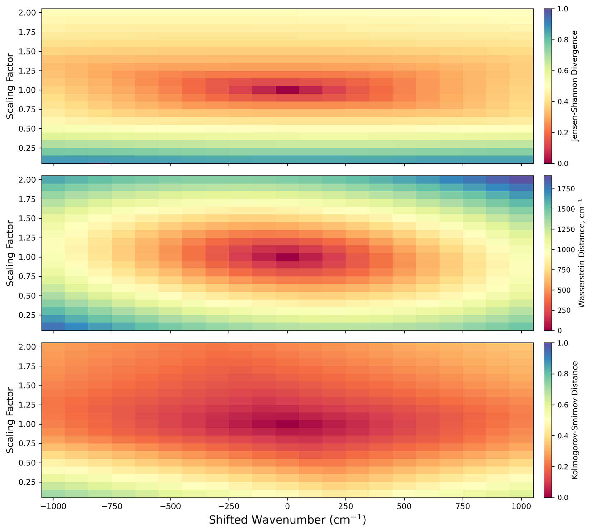
Figure 5 Distributions of Jensen–Shannon divergence (top panel), Wasserstein distance (middle panel), and Kolmogorov–Smirnov distance (bottom panel) as functions of scaling factor (from 0.1 to 2.0) and shifted wavenumber (from −1000 to +1000 cm⁻¹) for FY-4B/AGRI Channel 2 at 0.66 µm.

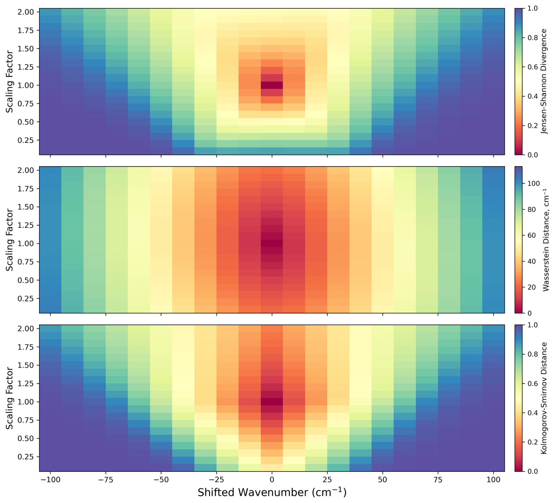
Figure 6 Same as Fig. 5, but for the FY-4B/AGRI Channel 13 at 10.80 µm with shifted wavenumber (from −100 to +100 cm⁻¹).

Moreover, both the VIS and IR channels of FY-4B/AGRI exhibit much greater sensitivity to variations in SRF width than to shifts in central wavenumber. When the SRF becomes narrower, all three similarity metrics mentioned above increase markedly (smaller values indicate greater similarity); for example, the JSD approaches 1.0. These results indirectly indicate that excessively large discrepancies in central wavelength and SRF width between the target and reference channels could seriously impair the effectiveness of the proposed transfer learning method.

3.2 Evaluation of Fitting Errors in Transfer Learning using Simulated SRFs

To more quantitatively evaluate the impact of SRF discrepancies, fitting experiments are conducted using both simulated SRFs and the original SRFs of FY-4B/AGRI mentioned before. The fitting errors in physics-constrained TL between reference and target channel radiance observations are calculated using simulated FY-4B/AGRI SRFs, with the following configurations: spectral width scaling factor from 0.1 to 2.0 (step 0.1); central wavelength shift from −100 to +100 cm⁻¹ (step 10 cm⁻¹) for IR channels, and from −1000 to +1000 cm⁻¹ (step 100 cm⁻¹) for VIS/NIR channels.

During the fitting process, the coefficient of determination (R²) is further used to determine whether a first-order linear fit or a second-order polynomial fit is more appropriate, and it is given by:

$$\begin{array}{}\text{(12)}& R^{\mathrm{2}}=\mathrm{1}-{\displaystyle \frac{{\sum }_{i=\mathrm{1}}^n{\left(y_i-{\widehat{y}}_i\right)}^{\mathrm{2}}}{{\sum }_{i=\mathrm{1}}^n{\left(y_i-\stackrel{\mathrm{‾}}{y}\right)}^{\mathrm{2}}}}\end{array}$$

where y, $\widehat{y}$, and $\stackrel{\mathrm{‾}}{y}$ denote the observed value, the fitted value, and the mean of the observed values, respectively. R² is commonly used to measure the extent to which the fitted model explains the variability in the observed data, with values closer to 1.0 indicating better agreement between fitted and observed values and stronger explanatory power of the model. In this study, a second-order polynomial fit is adopted when the R² value of the initial linear fit is below 0.95.

In addition, three metrics are used for assessing the fitting performance of the TL model, including the RMSE (root-mean-square-error), the correlation coefficient (R), and the number of outliers (N_outlier). They can be written as follows:

$$\begin{array}{}\text{(13)}& {\displaystyle }\mathrm{RMSE}=\sqrt{{\displaystyle \frac{\mathrm{1}}{n}}{\sum }_{i=\mathrm{1}}^n{\left(y_i-{\widehat{y}}_i\right)}^{\mathrm{2}}}\text{(14)}& {\displaystyle }R={\displaystyle \frac{{\sum }_{i=\mathrm{1}}^n\left(y_i-\stackrel{\mathrm{‾}}{y}\right)({\widehat{y}}_i-\stackrel{\mathrm{‾}}{\widehat{y}})}{\sqrt{{\sum }_{i=\mathrm{1}}^n{\left(y_i-\stackrel{\mathrm{‾}}{y}\right)}^{\mathrm{2}}}\sqrt{{\sum }_{i=\mathrm{1}}^n({\widehat{y}}_i-\stackrel{\mathrm{‾}}{\widehat{y}}{)}^{\mathrm{2}}}}}\end{array}$$

where $\stackrel{\mathrm{‾}}{\widehat{y}}$ denotes the mean of the fitted values. For the final metric, N_outlier, outliers are identified using the upper and lower fences. Any value lying beyond these two fences is regarded as an abnormal value, defined as:

$$\begin{array}{}\text{(15)}& {\displaystyle }{N}_{\mathrm{outlier}}=\left\{\begin{array}{l}{N}_{\mathrm{outlier}}^{\mathrm{UpperFence}}=Q_{\mathrm{75}}+\mathrm{1.5}\times \mathrm{IQR}\\ N_{\mathrm{outlier}}^{\mathrm{LowerFence}}=Q_{\mathrm{25}}-\mathrm{1.5}\times \mathrm{IQR}\end{array}\right.\text{(16)}& {\displaystyle }\mathrm{IQR}=Q_{\mathrm{75}}-Q_{\mathrm{25}}\end{array}$$

where Q₂₅ and Q₇₅ represent the 25th and 75th percentiles of the residuals, respectively. A higher outlier count (N_outlier) corresponds to an increased presence of extreme errors (or abnormal value).

Figure 7 shows the distributions of RMSE, R, and N_outlier as functions of scaling factor (0.1–2.0) and shifted wavenumber (−1000 to +1000 cm⁻¹) for FY-4B/AGRI Channel 2 (0.66 µm) and Channel 5 (1.61 µm). The results in the left panel for Channel 2 are generally consistent with those in Fig. 5: as the scaling factor increases, the discrepancy between the target and reference SRFs becomes larger, resulting in higher RMSE and N_outlier and a lower R. When the scaling factor exceeds 1.8, most cases require second-order polynomial fitting, suggesting that the relationship no longer follows a simple linear conversion. Notably, although scaling factors of about 0.1–0.2 correspond to large similarity differences in Fig. 5, they do not substantially degrade the TL performance, and the fitting remains predominantly linear. This may be because the narrower target channel still preserves particle scattering characteristics similar to those of the reference channel. By contrast, due to relatively low wavenumber, Channel 5 (1.61 µm) is much more sensitive to wavenumber shifts. Once the shift exceeds about 300 cm⁻¹, the RMSE increases significantly, the correlation coefficient decreases markedly, and both the fitting type and N_outlier exhibit abrupt changes.

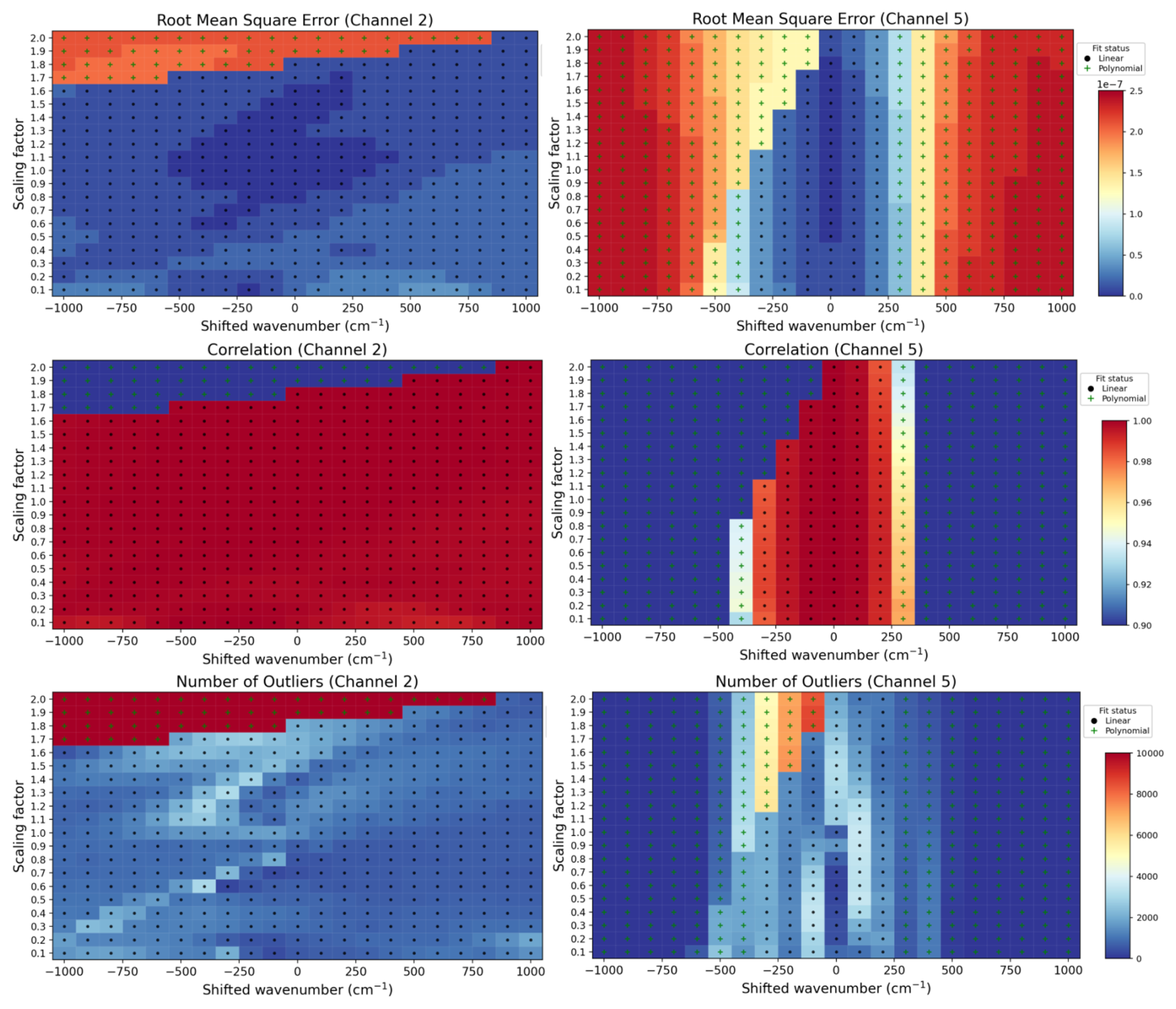
Figure 7 Distributions of RMSE (top panel), R (middle panel), and N_outlier (bottom panel) as functions of scaling factor (from 0.1 to 2.0) and shifted wavenumber (from −1000 to +1000 cm⁻¹) for FY-4B/AGRI Channel 2 at 0.66 µm (left panel) and Channel 5 at 1.61 µm (right panel). Black solid dots denote linear fits, and green plus signs denote polynomial fits, respectively, for each regression-based transfer learning model.

Figure 8 presents the results for FY-4B/AGRI Channel 9 (6.25 µm) and Channel 13 (10.80 µm). Channel 9 is a typical upper-tropospheric water vapor absorption channel, with its weighting function peaking around 300–400 hPa, corresponding to an altitude of approximately 8–9 km (Li et al., 2022). In terms of the correlation coefficient R, Channel 9 appears to be more sensitive to consistency in SRF shape. However, the RMSE results shown in the upper panels indicate that Channel 9 yields smaller fitting errors, suggesting that it is more suitable for observation radiance transfer by using the physics-constrained TL model. It is also noteworthy that, compared with the VIS/NIR channels discussed above (see Fig. 7), the IR channels produce N_outlier values about one order of magnitude smaller, indicating that particle scattering in the VIS/NIR bands introduces larger deviations into the TL performance.

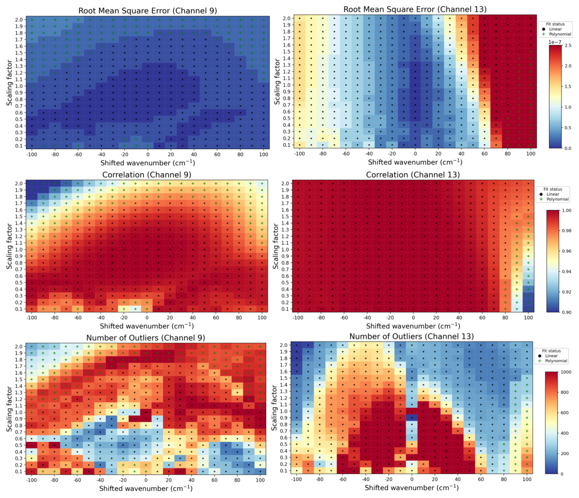
Figure 8 Same as Fig. 7, but for the FY-4B/AGRI Channel 9 at 6.25 µm (left panel) and Channel 13 at 10.80 µm (right panel).

The results of Figs. 7 and 8 indicate that the performance of the physics-constrained TL model is strongly affected by SRF discrepancies. Larger differences in scaling factor or shifted wavenumber generally lead to higher fitting errors, more outliers, and lower correlation, while IR channels show better transfer performance than VIS/NIR channels, likely because particle scattering introduces larger deviations in the latter. As a conservative guideline, for VIS/NIR channels, the difference in central wavenumber should be kept below 200 cm⁻¹, while the scaling factor should be constrained to the range of 0.5–1.5. In comparison, IR channels, particularly the water-vapor bands, appear to be somewhat more tolerant. However, for atmospheric window channels around 11 µm, the shifted wavenumber should ideally remain below 20 cm⁻¹, with the scaling factor likewise limited to 0.5–1.5. If the similarity between the target and reference channels is too low, reliable conversion becomes infeasible; the resulting conversion errors will then propagate into the retrieval model and further degrade retrieval performance. To facilitate practical application of the proposed framework, the empirical SRF-similarity guidelines derived from Figs. 7 and 8 are summarized by channel type in Table 2. These values should be interpreted as conservative screening criteria for the simulated SRF perturbations examined in this study, rather than as universal limits applicable to all satellite sensors.

Table 2 Empirical screening guidelines for SRF-based channel transferability in the physics-constrained TL framework.

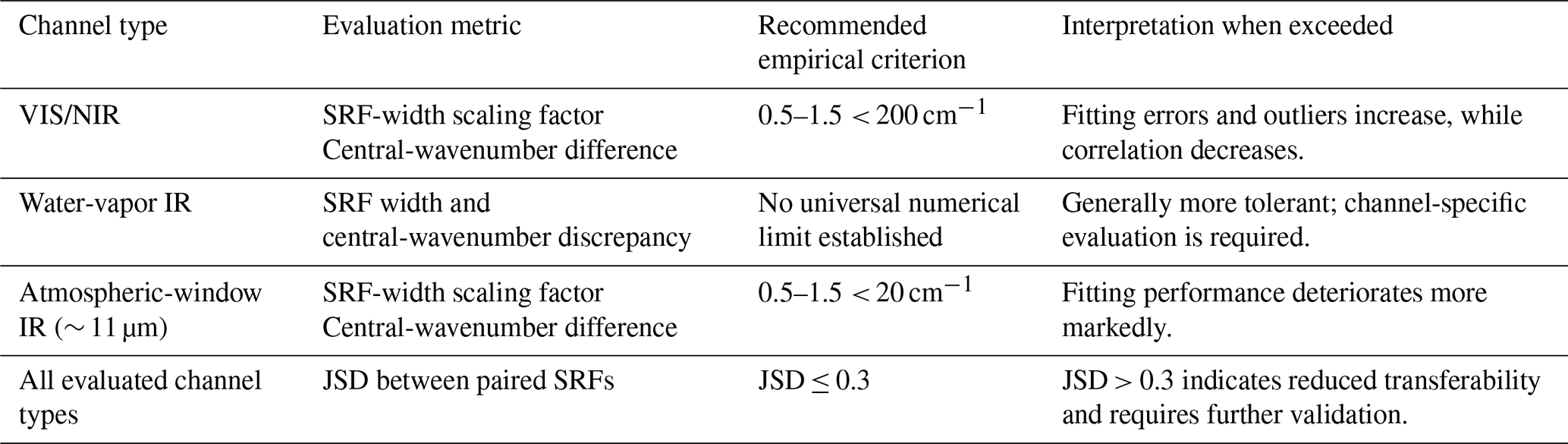
Note: These values represent empirical screening guidelines derived from the SRF-perturbation experiments in Figs. 7 and 8, rather than universal sensor-design limits.

Using the existing simulated convolution dataset, we evaluated the transfer performance of the 3.75 µm channel at the available discrete solar zenith angles. The analysis comprised 18 000 matched FY-4A and FY-4B Channel 07 samples drawn from five infrared atmospheric conditions. The relative RMSEs at solar zenith angles of 0, 30, and 60° were 2.020 %, 2.004 %, and 2.012 %, respectively, showing no monotonic degradation with increasing solar zenith angle within the simulation range. The relative RMSE varied modestly, ranging from approximately 1.82 % to 2.19 % across different viewing azimuth configurations. These results suggest that the total-radiance transfer relationship remains broadly stable over the daytime geometries examined. Nevertheless, this assessment should be viewed as an internal consistency analysis of the simulated transfer relationship, rather than an independent validation of solar-reflection correction or downstream retrieval accuracy.

3.3 Influence of Radiometric Calibration Uncertainties in Transfer Learning

Beyond SRF differences, radiometric calibration uncertainty in each target channel can also influence the stability and reliability of the physics-constrained TL model. We clarify the scope of the error-propagation derivation presented below. The propagation in Eqs. (17)–(21) and (A20)–(A21) takes the radiometric calibration uncertainty of the target channel (2 %–5 % in reflectance for VIS/NIR channels, Xiong et al., 2019; 0.1–1.0 K in brightness temperature for IR channels, He et al., 2021) as an externally imposed input and propagates it through the already-fitted TL model. Uncertainty associated with the fitted coefficients themselves, the SRF characterization, and the underlying RTM simulations is not included in this derivation and is assumed to be small relative to the imposed target-channel uncertainty. For consistency, throughout this section “error” and “uncertainty” are used interchangeably to denote the propagated standard deviation (σ), while “bias” refers specifically to the assumed radiometric calibration offset of the target channel that is propagated. According to Eq. (3) and Fig. 3, when the TL model is linear, i.e., $y=ax+b$, where a and b are fitted coefficients, and x and y denote the radiances in the target (FY-4B/AGRI) and reference (FY-4A/AGRI) channels, respectively, the associated error (σ, or uncertainty) propagation is obtained by differentiating the linear relationship, as follows:

$$\begin{array}{}\text{(17)}& {\mathit{\sigma }}_y=\left|a\right|\times {\mathit{\sigma }}_x.\end{array}$$

However, as shown in Fig. 3d (FY-4B/AGRI Channel 15 centered at 13.30 µm), when the TL model is nonlinear and represented by a quadratic function, i.e., $y=a{x}^{\mathrm{2}}+bx+c$, the corresponding error propagation can be expressed as follows (first-order approximation):

$$\begin{array}{}\text{(18)}& {\mathit{\sigma }}_y=|\mathrm{2}ax+b|\times {\mathit{\sigma }}_x.\end{array}$$

This equation suggests that the error in the reference-channel radiance (y) is strongly dependent on the magnitude of the radiance observed in the target channel (x).

According to Eq. (5), the propagation of uncertainties or errors in the reflectance observed by the VIS/NIR channels, which are typically on the order of 2 %–5 % (Xiong et al., 2019), can be readily expressed as follows:

$$\begin{array}{}\text{(19)}& {\mathit{\sigma }}_x=\left|{\displaystyle \frac{F_{\mathrm{0},\mathrm{t}}}{\mathit{\pi }}}\right|\times {\mathit{\sigma }}_{\mathit{\rho },\mathrm{t}}.\end{array}$$

By combining Eqs. (5), (17), (18), and (19), the reflectance errors (σ_ρ,r) in the reference channel with different fitting formula (Eqs. 17 and 18) can be expressed as follows:

$$\begin{array}{}\text{(20)}& {\displaystyle }{\mathit{\sigma }}_{\mathit{\rho },\mathrm{r}}=\left|a\right|\times \left|{\displaystyle \frac{F_{\mathrm{0},\mathrm{t}}}{F_{\mathrm{0},\mathrm{r}}}}\right|\times {\mathit{\sigma }}_{\mathit{\rho },\mathrm{t}}\text{(21)}& {\displaystyle }{\mathit{\sigma }}_{\mathit{\rho },\mathrm{r}}=|\mathrm{2}a{\displaystyle \frac{F_{\mathrm{0},\mathrm{t}}}{\mathit{\pi }}}{\mathit{\rho }}_{\mathrm{t}}+b|\times \left|{\displaystyle \frac{F_{\mathrm{0},\mathrm{t}}}{F_{\mathrm{0},\mathrm{r}}}}\right|\times {\mathit{\sigma }}_{\mathit{\rho },\mathrm{t}}\end{array}$$

where the footnotes of ρ, t, and r respectively signify the reflectance, target, and reference. It should be noted that the formulation of ρ_t does not explicitly include the term of cos(θ₀). According to Eq. (20), the propagation of reflectance error in ρ_t is controlled solely by the slope of the TL model and the solar irradiance terms of the two different channels. By comparison, the nonlinear form in Eq. (21) additionally depends on the reflectance observed by the target channel.

Compared with the VIS/NIR channels, the propagation of uncertainties (0.1 ∼ 1.0 K) (He et al., 2021) in the BTs measured in the target IR channels is nonlinear and more complex, owing to the additional Planck-function conversion and Planck-weighted correction calculation (Chen et al., 2012). In this study, the final equations for uncertainty propagation in the IR channels are given as Eqs. (A20) and (A21), with the full derivation provided in the Appendix A.

To address the inherent calibration-drift errors among different spectral channels, chain-rule-based error-propagation sensitivity experiments were conducted according to Eqs. (20), (21), (A20), and (A21). Figure 9 presents the heatmaps derived from the corresponding error-sensitivity analysis for the FY-4/AGRI sensors based on the physics-constrained TL models. Note that the A → B case in Fig. 9 follows the same target/reference assignment as Fig. 3 (FY-4A as the target, FY-4B as the reference), while the B → A case represents the reverse assignment, enabling a symmetric assessment of transfer errors in both directions. For the solar reflective channels, propagated errors are generally attenuated because the error-transfer relationship is predominantly linear, with absolute slopes smaller than unity. However, Channel 4 at 1.38 µm exhibits notably unstable behavior and pronounced error amplification. This channel is primarily sensitive to upper-level ice crystals and is widely used for cirrus cloud detection (Gao et al., 1993). In addition, as shown in Fig. 2, the SRF of FY-4B/AGRI Channel 4 (1.38 µm) covers a substantially narrower range than that of FY-4A/AGRI, which may directly result in a relatively large slope in the fitted TL model and, consequently, a larger difference between the two F₀ terms in Eq. (20). Regardless of the specific mechanism, Fig. 9 further indicates that when the radiometric calibration bias becomes large (e.g., reaching 6 %), the resulting transfer error also increases approximately linearly. In other words, channels subject to substantial radiometric calibration bias are not well suited for transfer-learning-based retrieval applications.

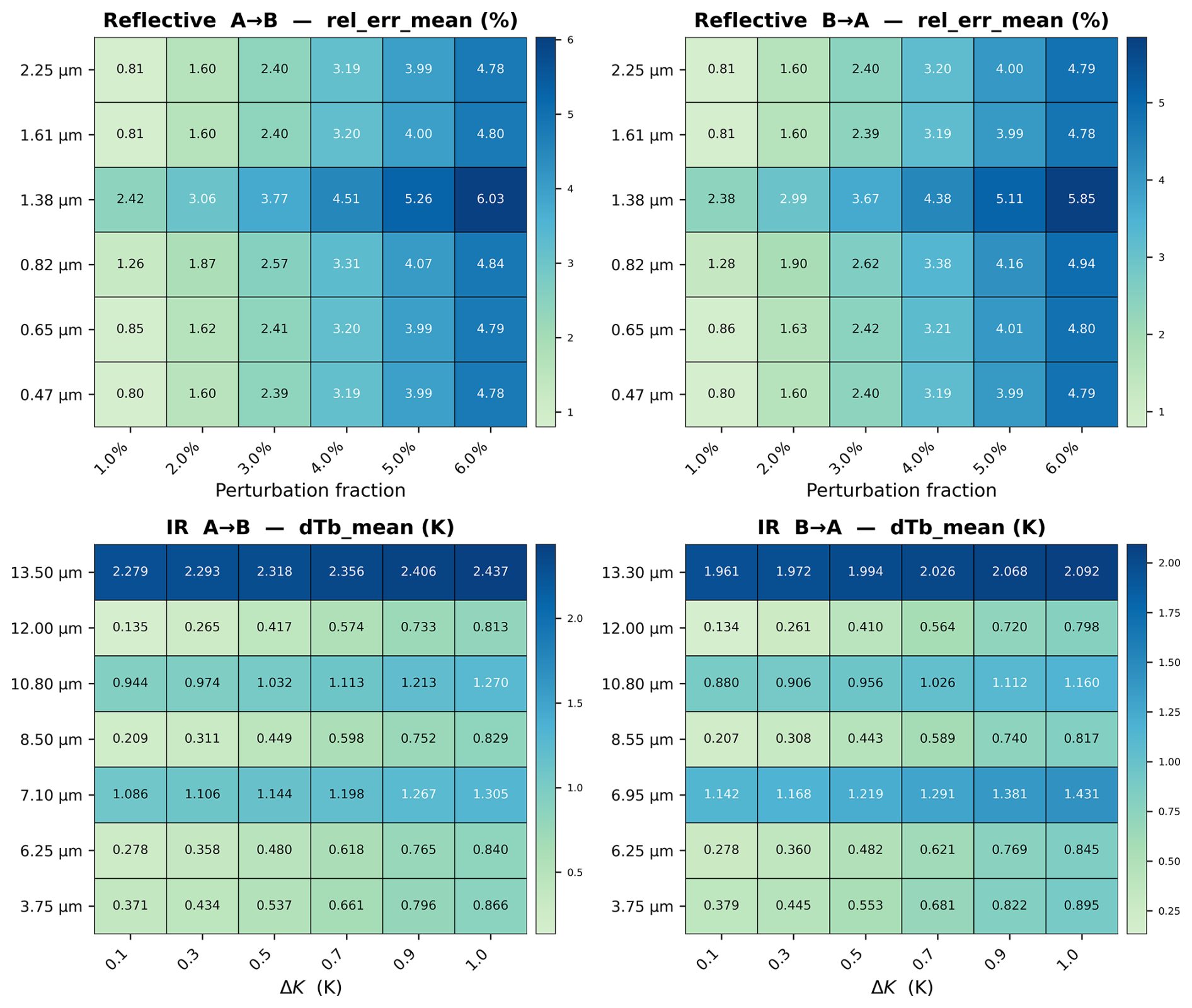
Figure 9 Heatmaps derived from the error-sensitivity analysis based on the physics-constrained TL models show error perturbations ranging from 1 % to 6 % in reflectance for the solar reflective channels and from 0.1 to 1 K within an interval of 0.2 K in brightness temperature for the thermal infrared emission channels. The A → B case (left panel) denotes the transformation in which FY-4A/AGRI channels are treated as the target channels and FY-4B/AGRI channels as the reference channels, whereas the B → A case (right panel) represents the exact reverse process.

In contrast, for most IR channels, small perturbations tend to be amplified, whereas larger perturbations remain close to the magnitude of the original input. A notable exception is FY-4A/AGRI Channel 14 (13.30 µm), which is modeled using a polynomial relationship (see Fig. 3d). The propagated errors for this channel are substantially amplified, owing to pronounced SRF discrepancies and its high sensitivity to atmospheric variability. In addition, the 7.10 and 10.80 µm channels exhibit relatively larger transfer errors because these bands underwent notable upgrades from FY-4A to FY-4B, whereas the remaining channels are generally more stable. Overall, although the IR channels involve a more complicated Planck-function-based conversion (see Eqs. A20 and A21), they are comparatively more stable and thus more suitable for TL applications. This is largely because onboard blackbody calibration constrains the radiometric biases of most IR channels to within about 0.5 K (Min et al., 2022; He et al., 2021), leading to perturbations of a similar magnitude. Relative to typical observed BTs of around 270 K, this corresponds to a relative error of only about 0.2 %, which is much smaller than that in the solar reflective channels (about 2 %–5 %).

4 Transfer-Learning-Based Satellite Retrieval Experiments

4.1 A Sensitivity Experiment on Retrieving Cloud Amount Profile

Lin et al. (2025) developed CLANN (Cloud Amount Neural Network), a ML framework designed to retrieve three-dimensional (3D) cloud amount profiles from observations acquired by the FY-4A geostationary meteorological satellite passive imager, with important applications in cloud climatology and weather analysis (Lin et al., 2025). The model integrates multi-channel observations from FY-4A/AGRI, including VIS/NIR (0.47, 0.66, and 0.86, 1.38, 1.61, and 2.25 µm), and IR channels (3.75, 6.25, 7.10, 8.60, 10.80, 12.00 µm), together with reanalysis-based environmental predictors. CALIPSO (Cloud-Aerosol Lidar and Infrared Pathfinder Satellite Observations)/CALIOP (Cloud-Aerosol Lidar with Orthogonal Polarization) cloud products from 1 March 2018 to 31 December 2020 were used as the reference for model training and independent evaluation. In essence, CLANN learns the vertical distribution of cloud amount from collocated passive-sensor radiances and environmental fields, thereby extending 3D cloud information beyond the narrow swath of active sensors. Validation results showed a correlation coefficient of 0.73 for cloud amount profile retrieval. In addition, the cloud-amount-weighted height derived from CLANN agreed well with CALIOP, with an RMSE of approximately 1.88 km and a correlation coefficient of 0.92. Feature-importance analysis further indicated that AGRI water-vapor-band observation BTs and upper-tropospheric temperature are among the most influential predictors for improving CLANN retrieval skill (Lin et al., 2025).

FY-4B did not enter operational service until December 2022 (Xia et al., 2025). By the time reliable FY-4B/AGRI observations became routinely available, CALIPSO observations had largely ceased in the second half of 2023, leaving only a limited period of effective overlap between FY-4B/AGRI and CALIPSO (approximately June 2022 to March 2023). Consequently, previous work did not attempt to develop an FY-4B/AGRI-based CLANN retrieval model. Nevertheless, this limited overlap provides an opportunity for a targeted evaluation of the physics-constrained TL model using the available collocated FY-4B/AGRI and CALIPSO observations. In the first control experiment, FY-4B/AGRI observations from channels corresponding to those used in CLANN training were directly ingested into the FY-4A/AGRI-based CLANN model mentioned above (Lin et al., 2025) to retrieve cloud amount profiles. In the second sensitivity experiment, the newly developed TL models (Fig. 3 and Table S1) were applied to convert each FY-4B/AGRI channel observation, in either reflectance (VIS/NIR) or BT (IR) form (reference), into its FY-4A/AGRI-equivalent value (target), which was then used as input to the CLANN model for estimating cloud amount profile. Finally, independent CALIPSO observations from 1 June 2022 to 31 March 2023, were used to comprehensively and accurately evaluate the effectiveness of the TL model.

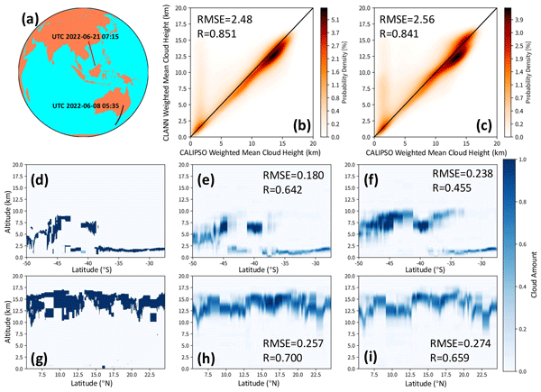
Figure 10 presents the cloud-amount-weighted mean height comparisons between CLANN (trained using FY-4A data) and CALIPSO based on FY-4B/AGRI observations, with and without the physics-constrained transfer learning model. As shown in Fig. 10b and c, the incorporation of the TL model produces a modest numerical reduction in RMSE of 0.08 km and increases the correlation coefficient from 0.841 to 0.851. Because the two correlations were calculated from the same 517 958 collocated CALIPSO–AGRI profile pairs and shared CALIPSO as the common reference variable, they were compared as dependent and overlapping correlations. The correlation between the retrievals obtained with and without TL was 0.927. At the individual-profile level, Zou's 99 % confidence interval for the increase in the correlation coefficient (ΔR= 0.010) was 0.0093–0.0107, excluding zero. Thus, the increase in R is statistically detectable at the profile level under the sampling assumptions of the test. However, neighboring profiles along the same CALIPSO track may exhibit spatial dependence, which was not explicitly accounted for in this analysis. The confidence interval should therefore not be interpreted as a fully dependence-adjusted assessment of statistical significance, and the reduction in RMSE is reported as a descriptive numerical change rather than a statistically significant difference. Although the R value remains lower than that achieved using FY-4A/AGRI data (R=0.92) (Lin et al., 2025), the results suggest a modest improvement within the available FY-4B validation period. In addition, cross-sectional cloud amount profiles for two representative cases (05:35 UTC on 8 June 2022, and 07:15 UTC on 21 June 2022) are presented in the middle and bottom panels, respectively. These cases qualitatively illustrate that the physics-constrained TL model can improve the representation of the vertical cloud amount distribution, but they are not regarded as independent evidence of statistical significance. The approximately 10-month validation period and the potential along-track dependence of neighboring profiles should be considered when interpreting the generalizability of these results.

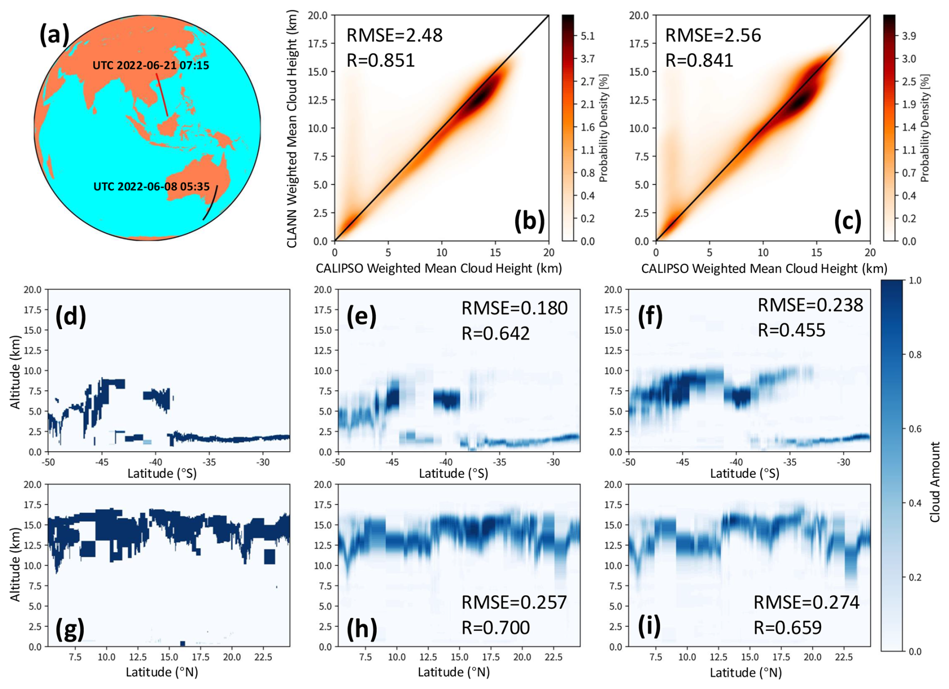
Figure 10 Map projection of CALIPSO tracks for two cases is shown in (a). Panels (b)–(c) present cloud-amount-weighted mean height comparisons between CLANN and CALIPSO using FY-4B/AGRI data, with and without TL model, respectively. Panels (d)–(i) show cross-sectional cloud amount profiles, including CALIPSO observations (d, g), CLANN with TL model (e, h), and without TL model (f, i). Cases 1 and 2 at 05:35 UTC on 8 June 2022 (black solid line) and 07:15 UTC on 21 June 2022 (red solid line), respectively. RMSE and correlation coefficients (R) are indicated in each panel.

4.2 A Sensitivity Experiment on Estimating Quantitative Precipitation

We also evaluate the impact of the physics-constrained TL model on quantitative precipitation estimation (QPE) using a Multi-Task UNet model (Ronneberger et al., 2015) trained on four FY-4A/AGRI IR channels (C09, C10, C12, and C13 at 6.25, 7.10, 10.80, 12.00 µm), with GPM (Global Precipitation Measurement) IMERG (Integrated Multi-satellitE Retrievals for GPM) products as the reference (Skofronick-Jackson et al., 2017). The FY-4A-based model was trained and validated using observations from 2019, with data from May to August used as the primary training period and randomly selected days from each of the remaining months included to ensure seasonal representativeness across both the validation and inference stages. The study domain covered 90–130° E and 0–40° N. To assess cross-satellite generalizability, three independent FY-4B/AGRI observation cases were selected from the extrapolation period spanning June 2023 to August 2024, which was entirely outside the FY-4A training window. These cases include Case 1 on 11 July 2024 at 09:15 UTC, Case 2 on 10 August 2024 at 00:00 UTC, and Case 3 on 12 July 2024.

Figure 11a–c and d–f show the spatial distributions of QPE results for Cases 1 and 2 mentioned above, respectively, including GPM IMERG rain rates, the raw FY-4B model output, and the TL corrected FY-4B output. Without TL correction, the raw FY-4B model systematically underestimates precipitation in both cases, producing substantially lower rain rates than GPM IMERG. The corresponding CSI (Critical Success Index) values are 0.392 and 0.412 for Cases 1 and 2, respectively. After applying the physics-constrained TL, the predicted precipitation fields become much more consistent with GPM IMERG, with the CSI increasing to 0.498 in both cases. This improvement indicates a robust and reproducible enhancement in precipitation detection skill.

Figure 11g–i further evaluate model performance using the FY-4A in-domain latitudinal rain-rate profile and scatter-density comparisons between the FY-4B model estimates and GPM IMERG. The FY-4A in-domain baseline (Fig. 11g; 15 May 2019), selected from the primary training period, achieves a CSI of 0.537, confirming the expected performance of the retrieval model under the original FY-4A observation domain. For the raw FY-4B configuration (Fig. 11h), the model yields R (correlation coefficient) = 0.462, MAE (Mean Absolute Error) = 1.678 mm h⁻¹, and bias = −0.959 mm h⁻¹, indicating a systematic underestimation when the FY-4A-trained model is directly applied to FY-4B observations without correction. The underestimation of precipitation, especially for extreme rainfall intensities, is a common issue in AI-based QPE models (Kühnlein et al., 2014a). After TL correction (Fig. 11i), R increases to 0.475, MAE decreases to 1.564 mm h⁻¹, and bias improves to −0.450 mm h⁻¹, demonstrating a reduction in systematic error.

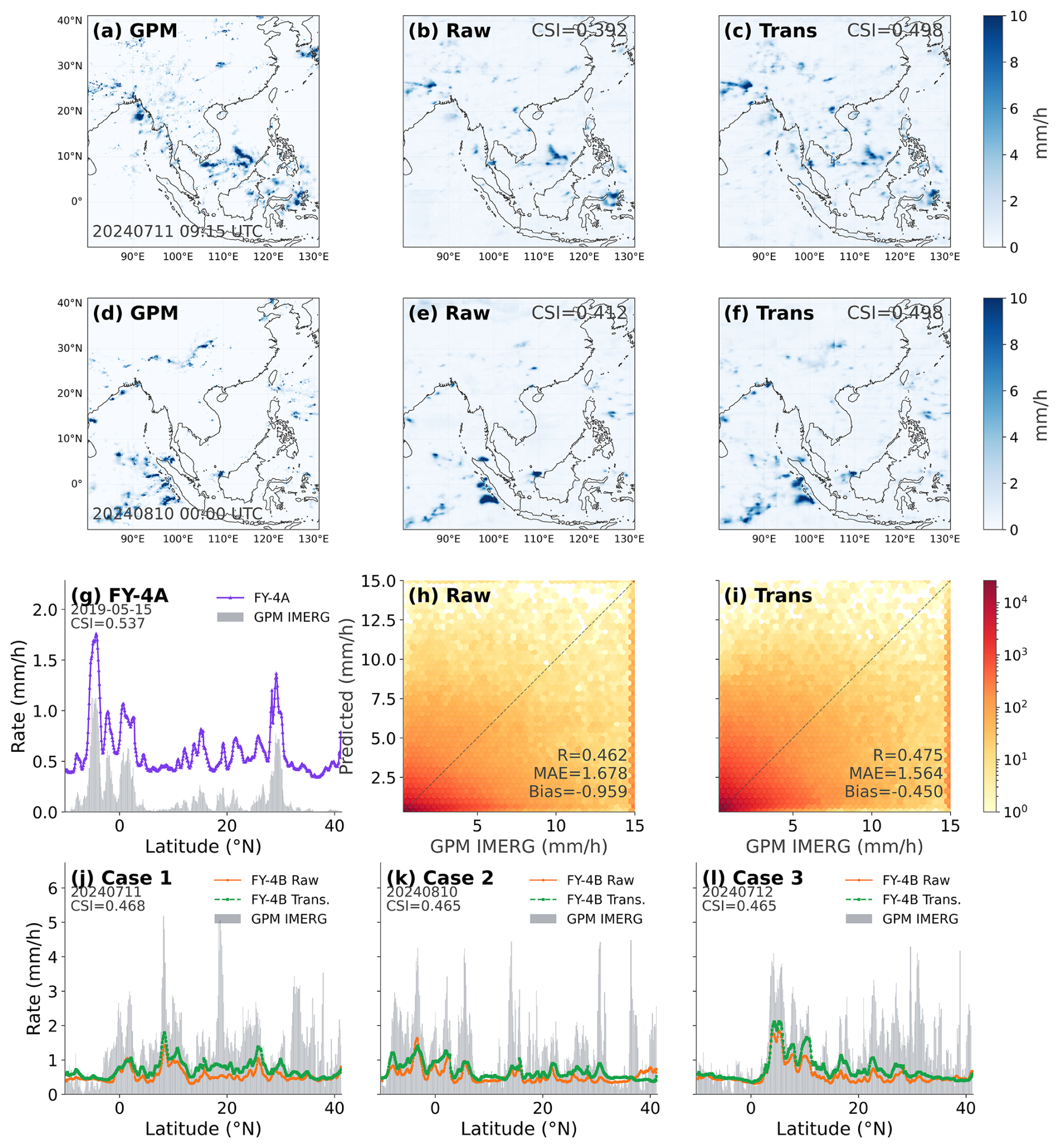
Figure 11 Evaluation of the physics-constrained transfer learning framework for QPE using a Multi-Task UNet model trained with 2019 FY-4A/AGRI observations. The training samples were mainly drawn from May–August and supplemented with five randomly selected days from each remaining month. (a–c) Spatial distributions of rain rate (mm h⁻¹) from GPM IMERG, the raw FY-4B output, and the transfer-learning-corrected FY-4B output for Case 1 on 11 July 2024 at 09:15 UTC. CSI values are annotated for the raw and corrected outputs. (d–f) Same as (a)–(c), but for Case 2 on 10 August 2024 at 00:00 UTC. (g) Latitudinal rain-rate profile for the FY-4A in-domain baseline on 15 May 2019. (h–i) Scatter-density comparisons between the raw FY-4B and TL-corrected FY-4B estimates and GPM IMERG rain rates, respectively. R, MAE, and bias are annotated in panels (h)–(i). (j–l) Latitudinal rain-rate profiles for Cases 1–3, corresponding to 11 July, 10 August, and 12 July 2024, respectively, comparing the raw FY-4B (orange solid line) output, TL-corrected FY-4B (green solid line) output, and GPM IMERG reference (gray). CSI values for the corrected output are annotated in each panel. All independent FY-4B cases were selected from the extrapolation period spanning June 2023 to August 2024, which is entirely outside the FY-4A training window.

The latitudinal rain-rate profiles in Fig. 11j–l further confirm the improvement across all three cases. The raw FY-4B model consistently underestimates the precipitation structure represented by GPM IMERG, whereas the transfer-learning-corrected FY-4B output better captures the overall latitudinal variability. The consistent improvement across Cases 1–3, which were selected from the FY-4B extrapolation period and span different months and meteorological conditions, demonstrates that the physics-constrained TL model can effectively recover the retrieval capability of the FY-4A-trained model when applied to FY-4B observations.

5 Discussions and Conclusions

This paper presents a recently developed physics-constrained TL framework for satellite remote sensing applications, which differs fundamentally from conventional AI-based TL approaches, offering strong physical interpretability and high generalization capability. The core of this physics-constrained TL framework is a Spectral-Fidelity-Preserving model built on extensive radiative transfer computations, enabling the transformation of radiance observations across different satellites and similar spectral channels spanning 0.47–13.5 µm. The TL is implemented using either linear or quadratic regression models, and the approach can be well applied to satellite radiometric calibration transfer, cross-satellite retrieval model adaptation, and related applications.

We further examine the quantitative effects of satellite channel SRF differences, including spectral width variations and central wavelength shifts, as well as radiometric uncertainties, on the accuracy of this physics-constrained transfer learning framework. To validate this approach, we performed some sensitivity experiments using a neural-network-based cloud amount profile retrieval model and a quantitative precipitation estimation model with transferred radiometric observations between FY-4A and FY-4B GEO satellite imagers. The results clearly demonstrate that the proposed physics-constrained TL technique improves the retrieval accuracy of key satellite-derived parameters.

However, from both theoretical and practical perspectives, several key issues regarding the applicability of this physics-constrained transfer learning framework need to be further investigated.

1. As described in Sect. 2, the core Spectral-Fidelity-Preserving model is constructed from extensive band-specific simulations spanning diverse atmospheric, surface, cloud, and viewing conditions. From a sample diversity perspective, there is currently no need to further increase the observation geometries or atmospheric conditions to enhance representativeness. The wide distribution of observed radiances shown in Fig. 3 also directly confirms the reliability of the training dataset. Compared with mainstream AI-based TL approaches (Ma et al., 2024), the proposed physics-constrained TL model exhibits distinct advantages. Only a single large-scale radiative transfer computation is required, after which the model can be applied conveniently. Users need only provide the SRFs of the target and reference satellite channels to rapidly fit the observation radiance transformation model of training quality, without undergoing the extensive retraining and testing process required by AI-based models. Consequently, the model demonstrates excellent generalization capability, eliminating the need for substantial computational resources for repeated modeling. As long as the SRFs of the satellite channels to be transferred fall within the 0.47–13.5 µm spectral range, the transformation model can be directly fitted. Notably, the core SFP model within this TL framework preserves the simulated information from satellite-based hyperspectral observations, encompassing physical processes such as atmospheric reflection and absorption, thereby effectively accounting for differences in fitting performance across channels.

   The present treatment retains both solar and thermal contributions within the total daytime radiance of the 3.75 µm channel, but does not explicitly separate the two components. Moreover, the current simulations adopt a Lambertian surface assumption and a fixed solar azimuth, and the retained infrared dataset samples only solar zenith angles of 0, 30, and 60°. Consequently, the reported angular performance pertains solely to the simulated conditions examined here and should not be construed as a general validation under arbitrary surface bidirectional reflectance, strong sun-glint, or unsampled illumination geometries.

2. As shown in Sect. 3, the proposed TL framework is most sensitive to differences in the SRFs among satellite channels. As detailed in Sect. 3.2, IR channels generally tolerate larger central-wavenumber shifts than VIS/NIR channels, with the notable exception of the atmospheric window region, where the same scaling-factor constraint but a stricter shift constraint applies. Prior to applying this transfer learning model, it is recommended to evaluate the SRF similarity between target and reference channels using metrics such as Jensen-Shannon divergence, Wasserstein distance, and Kolmogorov–Smirnov distance, as described in Sect. 3.2. The empirical analysis in Figs. 7–8 shows that when JSD ≤ 0.3, the RMSE remains low and R² > 0.95, while exceeding this threshold leads to a marked increase in fitting errors. Therefore, JSD ≤ 0.3 is recommended as an empirical threshold for channel transferability.

   In addition to SRF differences, radiometric calibration uncertainties of individual channels also affect TL model performance. Overall, the physics-constrained TL model is relatively insensitive to calibration uncertainties in IR channels (errors < 0.2 %). In contrast, errors in VIS/NIR channels propagate proportionally to their actual calibration uncertainties. State-of-the-art satellite imagers exhibit calibration errors of approximately 1.5 % in the VIS/NIR channels (Choi et al., 2024), an order of magnitude higher than for IR channels. This indicates that the use of this TL model requires particular caution when large calibration uncertainties are present in VIS/NIR channels.

3. Early radiometric calibration studies (Yu et al., 2026) have demonstrated that this TL model can propagate high-quality radiometric calibration standards from one satellite (reference) to lower-quality calibration channels on other satellites, primarily for VIS/NIR channels. In contrast, IR channels have traditionally relied on high-spectral-resolution IR imagers for synchronous nadir overpass (SNO) (Hewison et al., 2013) and error assessment. However, differences in horizontal spatial resolution between imaging instruments (0.25–1.0 km) and high-spectral infrared sounders (10–20 km) still introduce significant spatial uncertainties and noise when applying SNO techniques to polar-orbiting satellite imagers. The newly developed TL model presented in this study offers a novel approach for calibrating and evaluating IR channels on polar-orbiting satellites. The FY-4A/FY-4B experiments in Sect. 4 demonstrate spectral harmonization and retrieval-model transfer, whereas radiometric calibration transfer requires validation against an independent radiometric reference and was demonstrated in our previous FY-3D/MERSI-II study using MODIS.

   A key application scenario is the transfer of core geophysical parameter retrieval algorithms across satellites of the same generation or different generations. This scenario has been demonstrated in Sect. 4 with experiments on cloud amount profile and quantitative precipitation. Currently, the physics-constrained TL model is used to satellites with relatively low spatial resolution, and its extension to higher-resolution Earth-observing satellites (e.g., Sentinel-2, Drusch et al., 2012) requires caution. At higher spatial resolutions, atmospheric radiative transfer calculations based on the plane-parallel approximation can introduce distortions, representing a primary limitation and bottleneck of the TL model.

Finally, the physics-constrained TL framework developed in this study is fully open-source and freely available for satellite channels spanning the VIS to IR spectral range (from 0.47 to 13.5 µm). Due to the extremely large size of the radiative transfer simulation dataset, it cannot be uploaded to online repositories. Researchers interested in using this physics-constrained TL tool can contact the first (Min Min, minm5@mail.sysu.edu.cn) or corresponding authors to obtain assistance in generating the relevant TL models.

Appendix A

The Planck-weighted correction method (Chen et al., 2012) likewise employs a linear form, $T_{\mathrm{b},\mathrm{t}}=S_{\mathrm{t}}\cdot T_{\mathrm{b},\mathrm{0}}+Q_{\mathrm{t}}$, in which T_b,t and T_b,0 respectively represent the brightness temperature (BT) observed by the satellite target IR channel and the corrected BT for the calculation using the Planck function, respectively. By contrast, for the reference IR channel, the observed BT is also corrected using a linear relationship, $T_{\mathrm{b},\mathrm{r}}=S_{\mathrm{r}}\cdot T_{\mathrm{b},\mathrm{1}}+Q_{\mathrm{r}}$. As in Eq. (17), the corresponding error propagation can be formulated as follows:

$$\begin{array}{}\text{(A1)}& {\displaystyle }{\mathit{\sigma }}_{T_{\mathrm{b},\mathrm{0}}}=\left|{\displaystyle \frac{\mathrm{1}}{S_{\mathrm{t}}}}\right|\times {\mathit{\sigma }}_{T_{\mathrm{b},\mathrm{t}}}\text{(A2)}& {\displaystyle }{\mathit{\sigma }}_{T_{\mathrm{b},\mathrm{r}}}=\left|S_{\mathrm{r}}\right|\times {\mathit{\sigma }}_{T_{\mathrm{b},\mathrm{1}}}\end{array}$$

For a given wavelength λ, the Planck function for radiance is expressed as:

$$\begin{array}{}\text{(A3)}& L_{\mathit{\lambda }}\left(T_{\mathrm{b},\mathrm{0}}\right)={\displaystyle \frac{c_{\mathrm{1}}}{{\mathit{\lambda }}^{\mathrm{5}}}}{\displaystyle \frac{\mathrm{1}}{\left[\exp \left(\frac{c_{\mathrm{2}}}{\mathit{\lambda }{T}_{\mathrm{b},\mathrm{0}}}\right)-\mathrm{1}\right]}}\end{array}$$

where c₁ (= 1.1910439×10⁻¹⁶ (W m² sr⁻¹)) and c₂ (= 1.438769 × 10⁻² (m K)) are the constants in the Planck function. To obtain $\frac{\mathrm{d}{L}_{\mathit{\lambda }}}{\mathrm{d}{T}_{\mathrm{b},\mathrm{0}}}$, we first define:

$$\begin{array}{}\text{(A4)}& {\displaystyle }u={\displaystyle \frac{c_{\mathrm{2}}}{\mathit{\lambda }{T}_{\mathrm{b},\mathrm{0}}}}\text{(A5)}& {\displaystyle \frac{\mathrm{d}u}{\mathrm{d}{T}_{\mathrm{b},\mathrm{0}}}}=-{\displaystyle \frac{c_{\mathrm{2}}}{\mathit{\lambda }{T}_{\mathrm{b},\mathrm{0}}^{\mathrm{2}}}}\end{array}$$

Then, the Eq. (A3) and $\frac{\mathrm{d}{L}_{\mathit{\lambda }}}{\mathrm{d}{T}_{\mathrm{b},\mathrm{0}}}$ are transformed into

$$\begin{array}{}\text{(A6)}& {\displaystyle }{L}_{\mathit{\lambda }}={\displaystyle \frac{c_{\mathrm{1}}}{{\mathit{\lambda }}^{\mathrm{5}}}}{\left(e^{\mathrm{u}}-\mathrm{1}\right)}^{-\mathrm{1}}\text{(A7)}& {\displaystyle \frac{\mathrm{d}{L}_{\mathit{\lambda }}}{\mathrm{d}{T}_{\mathrm{b},\mathrm{0}}}}={\displaystyle \frac{c_{\mathrm{1}}}{{\mathit{\lambda }}^{\mathrm{5}}}}\left[-{\left(e^u-\mathrm{1}\right)}^{-\mathrm{2}}{e}^u{\displaystyle \frac{\mathrm{d}u}{\mathrm{d}{T}_{\mathrm{b},\mathrm{0}}}}\right]\end{array}$$

By substituting Eqs. (A4) and (A5) into Eq. (A7), we obtain:

$$\begin{array}{}\text{(A8)}& {\displaystyle \frac{\mathrm{d}{L}_{\mathit{\lambda }}}{\mathrm{d}{T}_{\mathrm{b},\mathrm{0}}}}={\displaystyle \frac{c_{\mathrm{1}}{c}_{\mathrm{2}}}{{\mathit{\lambda }}^{\mathrm{6}}{T}_{\mathrm{b},\mathrm{0}}^{\mathrm{2}}}}{\displaystyle \frac{\exp \left(\frac{c_{\mathrm{2}}}{\mathit{\lambda }{T}_{\mathrm{b},\mathrm{0}}}\right)}{{\left[\exp \left(\frac{c_{\mathrm{2}}}{\mathit{\lambda }{T}_{\mathrm{b},\mathrm{0}}}\right)-\mathrm{1}\right]}^{\mathrm{2}}}}\end{array}$$

Therefore, according to the first-order error propagation formula, the propagation of observed-radiance errors (${\mathit{\sigma }}_{L_{\mathit{\lambda },\mathrm{t}}}$) (Here, we use L_λ,t to replace L_λ in Eq. A8) from T_b,t and T_b,0 can be expressed as follows:

$$\begin{array}{}\text{(A9)}& \begin{array}{rl}{\mathit{\sigma }}_{L_{\mathit{\lambda },\mathrm{t}}}& =\left|{\displaystyle \frac{c_{\mathrm{1}}{c}_{\mathrm{2}}}{{\mathit{\lambda }}^{\mathrm{6}}{T}_{\mathrm{b},\mathrm{0}}^{\mathrm{2}}}}{\displaystyle \frac{\exp \left(\frac{c_{\mathrm{2}}}{\mathit{\lambda }{T}_{\mathrm{b},\mathrm{0}}}\right)}{{\left[\exp \left(\frac{c_{\mathrm{2}}}{\mathit{\lambda }{T}_{\mathrm{b},\mathrm{0}}}\right)-\mathrm{1}\right]}^{\mathrm{2}}}}\right|\times {\mathit{\sigma }}_{T_{\mathrm{b},\mathrm{0}}}\\ & =\left|{\displaystyle \frac{c_{\mathrm{1}}{c}_{\mathrm{2}}}{{\mathit{\lambda }}^{\mathrm{6}}{\left[\left(T_{\mathrm{b},\mathrm{t}}-Q_{\mathrm{t}}\right)/S_{\mathrm{t}}\right]}^{\mathrm{2}}}}{\displaystyle \frac{\exp \left(\frac{c_{\mathrm{2}}}{\mathit{\lambda }\left[\left(T_{\mathrm{b},\mathrm{t}}-Q_{\mathrm{t}}\right)/S_{\mathrm{t}}\right]}\right)}{{\left[\exp \left(\frac{c_{\mathrm{2}}}{\mathit{\lambda }\left[\left(T_{\mathrm{b},\mathrm{t}}-Q_{\mathrm{t}}\right)/S_{\mathrm{t}}\right]}\right)-\mathrm{1}\right]}^{\mathrm{2}}}}\right|\\ & \times \left|{\displaystyle \frac{\mathrm{1}}{S_{\mathrm{t}}}}\right|\times {\mathit{\sigma }}_{T_{\mathrm{b},\mathrm{t}}}\end{array}\end{array}$$

In turn, the propagation of radiance error (L_λ) into the calculated BT (T_b,1) can be expressed in terms of $\frac{\mathrm{d}{T}_{\mathrm{b},\mathrm{1}}}{\mathrm{d}{L}_{\mathit{\lambda }}}$. The inverse of the Planck function in Eq. (A3) can be written as:

$$\begin{array}{}\text{(A10)}& T_{\mathrm{b},\mathrm{1}}\left(L_{\mathit{\lambda }}\right)={\displaystyle \frac{{\mathrm{c}}_{\mathrm{2}}}{\mathit{\lambda }\cdot \ln \left(\mathrm{1}+\frac{c_{\mathrm{1}}}{{\mathit{\lambda }}^{\mathrm{5}}{L}_{\mathit{\lambda }}}\right)}}\end{array}$$

Then, we first define:

$$\begin{array}{}\text{(A11)}& {\displaystyle }A={\displaystyle \frac{c_{\mathrm{1}}}{{\mathit{\lambda }}^{\mathrm{5}}}}\text{(A12)}& {\displaystyle }u=\ln \left(\mathrm{1}+{\displaystyle \frac{\mathrm{A}}{L_{\mathit{\lambda }}}}\right)\text{(A13)}& {\displaystyle \frac{\mathrm{d}u}{\mathrm{d}{L}_{\mathit{\lambda }}}}={\displaystyle \frac{\mathrm{1}}{\mathrm{1}+A/L_{\mathit{\lambda }}}}\cdot {\displaystyle \frac{\mathrm{d}\left(A/L_{\mathit{\lambda }}\right)}{\mathrm{d}{L}_{\mathit{\lambda }}}}={\displaystyle \frac{\mathrm{1}}{\mathrm{1}+A/L_{\mathit{\lambda }}}}\left(-{\displaystyle \frac{A}{L_{\mathit{\lambda }}^{\mathrm{2}}}}\right).\end{array}$$

By substituting Eqs. (A11) and (A12) into Eq. (A10), we obtain:

$$\begin{array}{}\text{(A14)}& {\displaystyle }{T}_{\mathrm{b},\mathrm{1}}={\displaystyle \frac{{\mathrm{c}}_{\mathrm{2}}}{\mathit{\lambda }\cdot u}}\text{(A15)}& {\displaystyle \frac{\mathrm{d}{T}_{\mathrm{b},\mathrm{1}}}{\mathrm{d}{L}_{\mathit{\lambda }}}}=-{\displaystyle \frac{{\mathrm{c}}_{\mathrm{2}}}{\mathit{\lambda }\cdot u^{\mathrm{2}}}}{\displaystyle \frac{\mathrm{d}u}{\mathrm{d}{L}_{\mathit{\lambda }}}}\end{array}$$

Then, we substitute Eq. (A13) into Eq. (A15), we obtain:

$$\begin{array}{}\text{(A16)}& {\displaystyle \frac{\mathrm{d}{T}_{\mathrm{b},\mathrm{1}}}{\mathrm{d}{L}_{\mathit{\lambda }}}}={\displaystyle \frac{c_{\mathrm{2}}}{\mathit{\lambda }{u}^{\mathrm{2}}}}{\displaystyle \frac{A}{L_{\mathit{\lambda }}^{\mathrm{2}}(\mathrm{1}+A/L_{\mathit{\lambda }})}}\end{array}$$

Finally, by rearranging Eq. (A16), we obtain:

$$\begin{array}{}\text{(A17)}& {\displaystyle \frac{\mathrm{d}{T}_{\mathrm{b},\mathrm{1}}}{\mathrm{d}{L}_{\mathit{\lambda }}}}={\displaystyle \frac{c_{\mathrm{1}}{c}_{\mathrm{2}}/{\mathit{\lambda }}^{\mathrm{6}}}{L_{\mathit{\lambda }}\left(L_{\mathit{\lambda }}+\frac{c_{\mathrm{1}}}{{\mathit{\lambda }}^{\mathrm{5}}}\right){\left[\ln \left(\mathrm{1}+\frac{c_{\mathrm{1}}}{{\mathit{\lambda }}^{\mathrm{5}}{L}_{\mathit{\lambda }}}\right)\right]}^{\mathrm{2}}}}\end{array}$$

At this stage, the TL model established in this study is applied to L_λ,t to derive the transformed radiance of the reference IR channel, L_λ,r. As described in Sect. 3.3, for both the linear and quadratic nonlinear TL models, the corresponding error propagation based on Eq. (A17) can be expressed as follows:

$$\begin{array}{}\text{(A18)}& {\displaystyle }\begin{array}{rl}& {\mathit{\sigma }}_{T_{\mathrm{b},\mathrm{r}}}=\left|S_{\mathrm{r}}\right|\times {\mathit{\sigma }}_{T_{\mathrm{b},\mathrm{1}}}=\left|S_{\mathrm{r}}\right|\\ & \times \left|{\displaystyle \frac{c_{\mathrm{1}}{c}_{\mathrm{2}}a/{\mathit{\lambda }}^{\mathrm{6}}}{\left(ax+b\right)\left(ax+b+\frac{c_{\mathrm{1}}}{{\mathit{\lambda }}^{\mathrm{5}}}\right){\left[\ln \left(\mathrm{1}+\frac{c_{\mathrm{1}}}{{\mathit{\lambda }}^{\mathrm{5}}\left(ax+b\right)}\right)\right]}^{\mathrm{2}}}}\right|\times {\mathit{\sigma }}_x\end{array}\text{(A19)}& {\displaystyle }\begin{array}{rl}& {\mathit{\sigma }}_{T_{\mathrm{b},\mathrm{r}}}=\left|S_{\mathrm{r}}\right|\times {\mathit{\sigma }}_{T_{\mathrm{b},\mathrm{1}}}=\left|S_{\mathrm{r}}\right|\\ & \times \left|{\displaystyle \frac{c_{\mathrm{1}}{c}_{\mathrm{2}}\left(\mathrm{2}ax+b\right)/{\mathit{\lambda }}^{\mathrm{6}}}{\left(a{x}^{\mathrm{2}}+bx+c\right)\left(a{x}^{\mathrm{2}}+bx+c+\frac{c_{\mathrm{1}}}{{\mathit{\lambda }}^{\mathrm{5}}}\right){\left[\ln \left(\mathrm{1}+\frac{c_{\mathrm{1}}}{{\mathit{\lambda }}^{\mathrm{5}}\left(a{x}^{\mathrm{2}}+bx+c\right)}\right)\right]}^{\mathrm{2}}}}\right|\\ & \times {\mathit{\sigma }}_x\end{array}\end{array}$$

where x is the radiance (L_λ,t) observed by target IR channel in Eq. (A9).

According to the equations in Sect. 3.3, by combining Eqs. (A9), (A18), and (A19), the error propagation from the initially observed BT (T_b,t) in the target IR channel to the BT (T_b,r) observed by the final reference IR channel used as model input can be expressed as follows:

$$\begin{array}{}\text{(A20)}& {\displaystyle }\begin{array}{rl}{\mathit{\sigma }}_{T_{\mathrm{b},\mathrm{r}}}& =\left|{\displaystyle \frac{S_{\mathrm{r}}}{S_{\mathrm{t}}}}\right|\times \left|{\displaystyle \frac{c_{\mathrm{1}}{c}_{\mathrm{2}}a/{\mathit{\lambda }}^{\mathrm{6}}}{\left(ax+b\right)\left(ax+b+\frac{c_{\mathrm{1}}}{{\mathit{\lambda }}^{\mathrm{5}}}\right){\left[\ln \left(\mathrm{1}+\frac{c_{\mathrm{1}}}{{\mathit{\lambda }}^{\mathrm{5}}\left(ax+b\right)}\right)\right]}^{\mathrm{2}}}}\right|\\ & \times \left|{\displaystyle \frac{c_{\mathrm{1}}{c}_{\mathrm{2}}}{{\mathit{\lambda }}^{\mathrm{6}}{\left[\left(T_{\mathrm{b},\mathrm{t}}-Q_{\mathrm{t}}\right)/S_{\mathrm{t}}\right]}^{\mathrm{2}}}}{\displaystyle \frac{\exp \left(\frac{c_{\mathrm{2}}}{\mathit{\lambda }\left[\left(T_{\mathrm{b},\mathrm{t}}-Q_{\mathrm{t}}\right)/S_{\mathrm{t}}\right]}\right)}{{\left[\exp \left(\frac{c_{\mathrm{2}}}{\mathit{\lambda }\left[\left(T_{\mathrm{b},\mathrm{t}}-Q_{\mathrm{t}}\right)/S_{\mathrm{t}}\right]}\right)-\mathrm{1}\right]}^{\mathrm{2}}}}\right|\\ & \times {\mathit{\sigma }}_{T_{\mathrm{b},\mathrm{t}}}\end{array}\text{(A21)}& {\displaystyle }\begin{array}{rl}& {\mathit{\sigma }}_{T_{\mathrm{b},\mathrm{r}}}=\left|{\displaystyle \frac{S_{\mathrm{r}}}{S_{\mathrm{t}}}}\right|\\ & \times \left|{\displaystyle \frac{c_{\mathrm{1}}{c}_{\mathrm{2}}\left(\mathrm{2}ax+b\right)/{\mathit{\lambda }}^{\mathrm{6}}}{\left(a{x}^{\mathrm{2}}+bx+c\right)\left(a{x}^{\mathrm{2}}+bx+c+\frac{c_{\mathrm{1}}}{{\mathit{\lambda }}^{\mathrm{5}}}\right){\left[\ln \left(\mathrm{1}+\frac{c_{\mathrm{1}}}{{\mathit{\lambda }}^{\mathrm{5}}\left(a{x}^{\mathrm{2}}+bx+c\right)}\right)\right]}^{\mathrm{2}}}}\right|\\ & \times \left|{\displaystyle \frac{c_{\mathrm{1}}{c}_{\mathrm{2}}}{{\mathit{\lambda }}^{\mathrm{6}}{\left[\left(T_{\mathrm{b},\mathrm{t}}-Q_{\mathrm{t}}\right)/S_{\mathrm{t}}\right]}^{\mathrm{2}}}}{\displaystyle \frac{\exp \left(\frac{c_{\mathrm{2}}}{\mathit{\lambda }\left[\left(T_{\mathrm{b},\mathrm{t}}-Q_{\mathrm{t}}\right)/S_{\mathrm{t}}\right]}\right)}{{\left[\exp \left(\frac{c_{\mathrm{2}}}{\mathit{\lambda }\left[\left(T_{\mathrm{b},\mathrm{t}}-Q_{\mathrm{t}}\right)/S_{\mathrm{t}}\right]}\right)-\mathrm{1}\right]}^{\mathrm{2}}}}\right|\times {\mathit{\sigma }}_{T_{\mathrm{b},\mathrm{t}}}\end{array}\end{array}$$

where x is calculated from the Planck function in Eq. (A3). a, b, and c represent the fitted coefficients of the IR channel TL model introduced above. We will also use the derived error-propagation Eqs. (A20) and (A21) to conduct sensitivity experiments in Sect. 3.3.