Thermodynamics-guided machine learning model for predicting convective boundary layer height and its multi-site applicability

Accurate estimation of convective boundary layer height (CBLH) is vital for weather, climate, and air quality modeling. Machine learning (ML) shows promise in CBLH prediction, but input parameter selection often lacks physical grounding, limiting generalizability. This study introduces a novel ML framework for CBLH prediction, integrating thermodynamic constraints and the diurnal CBLH cycle as an implicit physical guide. Boundary layer growth is modeled as driven by surface heat fluxes and atmospheric heat absorption represented with the low tropospheric stability, using the diurnal cycle as input and output. TPOT and AutoKeras are employed to select optimal models, validated against Doppler lidar-derived CBLH data, achieving an R² of 0.84 across untrained years. Comparisons of eddy covariance (ECOR) and energy balance Bowen ratio (EBBR) flux measurements show the same prediction capability. Models trained on the ARM SGP C1 site with ECOR data and tested at E37 and E39 yield R² values of 0.79 and 0.81, respectively, demonstrating their adaptability. The ML model trained with all sites' data slightly enhances the performance compared with ML models trained over single-site data. The interquartile range for predicted CBLH is consistently narrower than that for DL-derived CBLH, reflecting lower variability in predicted CBLH compared to DL-derived CBLH, which is influenced by additional factors, which are not well represented with the model inputs. The model's generalizability across multiple sites at the ARM SGP site demonstrates its potential for transfer to greater distances, offering a scalable approach for enhancing boundary layer parameterization in atmospheric models.

1 Introduction

The convective boundary layer (CBL) is a critical component of the Earth's atmosphere, governing the exchange of heat, moisture, and momentum between the surface and the free troposphere (Stull, 1988; Garratt, 1994). Accurate estimation of the CBL height (CBLH) is essential for understanding atmospheric processes, including turbulence, pollutant dispersion, and cloud formation (Stull, 1988; Seibert et al., 2000). In numerical weather prediction (NWP) and climate models, CBLH serves as a key parameter for parameterizing turbulent mixing and convective processes, directly impacting forecast accuracy and climate projections (Grenier and Bretherton, 2001; Holtslag et al., 2013; Baklanov et al., 2014). Errors in CBLH estimation can lead to significant biases in surface temperature, humidity, and air quality predictions (Vogelezang and Holtslag, 1996; Hu et al., 2010). Consequently, improving CBLH predictions has been a priority in atmospheric science, with numerous studies emphasizing its role in model performance and data assimilation (Helmis et al., 2012; Cohen et al., 2015; Wulfmeyer and Turner, 2016; Brown et al., 2008; Barlow et al., 2015; Chu et al., 2022; Teixeira et al., 2025).

While current observational techniques have greatly contributed to the determination of the CBLH, each method still presents inherent limitations related to resolution, sensitivity, or applicability under different atmospheric conditions. Radiosondes provide direct measurements of temperature and humidity profiles but suffer from low temporal resolution, typically limited to twice to fourth-daily launches (Seidel et al., 2010; Liu and Liang, 2010; Lin et al., 2024). Meteorological towers measure near-surface variables but are constrained by their height, rarely capturing the full CBL (Bianco et al., 2011; Emeis et al., 2009). Weather radars offer vertical profiles but lack the resolution to resolve fine-scale CBL structures (Heo et al., 2003; Compton et al., 2013). Aerosol lidars, while effective for detecting entrainment zones, are often confounded by residual layers, leading to ambiguous CBLH estimates (Hennemuth and Lammert, 2006; Sawyer and Li, 2013; Schween et al., 2014; Luo et al., 2014). Doppler lidars provide high-resolution velocity and backscatter data, enabling precise CBLH retrievals, but their algorithms vary widely (Tucker et al., 2009; Barlow et al., 2011; Chu et al., 2020). Each method employs different inversion algorithms – such as gradient-based, variance-based, or wavelet techniques – each with inherent uncertainties depending on atmospheric conditions and data quality (Cohn and Angevine, 2000; Hägeli et al., 2000; Lammert and Bösenberg, 2006; Compton et al., 2013; Chu et al., 2022).

Recent advances in machine learning (ML) have revolutionized CBLH prediction by leveraging large datasets to model complex atmospheric relationships. Early ML approaches used simple regression models to estimate CBLH from radiosonde data (Krishnamurthy et al., 2021a; Madonna et al., 2021). Subsequent studies adopted random forests and neural networks, incorporating inputs from aerosol lidars, Doppler lidars, and reanalysis datasets (Liu et al., 2022; Krishnamurthy et al., 2021b; Peng et al., 2023; Wei et al., 2025; Zhang et al., 2025). For instance, random forest models have been applied to lidar-derived backscatter profiles (Du et al., 2020; Chu et al., 2025a), while deep neural networks have integrated reanalysis data for regional CBLH predictions (Ayazpour et al., 2023; Su and Zhang, 2024). Despite these advances, most ML models select input parameters empirically, lacking physical constraints, which limits their generalizability across diverse sites (de Arruda Moreira et al., 2022; Su and Zhang, 2024; Chu et al., 2025a; Macatangay et al., 2025; Stapleton et al., 2025). Few studies have explored physically constrained ML frameworks or evaluated model performance across multiple stations, highlighting a critical gap in the literature (Krishnamurthy et al., 2021b; Su and Zhang, 2024; Wei et al., 2025; Stapleton et al., 2025). Evaluating numerous ML algorithms to identify the optimal one is still highly time-consuming.

Building on these insights, this study introduces an Auto-ML framework that automatically selects the optimal ML algorithm for CBLH prediction, utilizing Doppler lidar-derived CBLH data and thermodynamically constrained input parameters, including sensible heat flux (SHF), latent heat flux (LHF), and lower tropospheric stability (LTS). Daily CBL evolution is mainly driven by SHF and LHF, atmospheric heat absorption and constrained by low tropospheric temperature. Thus, these thermodynamical inputs offer physical constrains to predict CBL growth. This approach ensures robust predictions across varying atmospheric conditions and sites. To assess the model's transferability, we evaluate its performance at four sub-sites (C1, E32, E37, and E39) within the Atmospheric Radiation Measurement (ARM) Southern Great Plains (SGP) supersite. These locations were selected due to their comprehensive observations of SHF, LHF, and LTS. These sites provide a diverse testbed for validating the model's generalizability and its potential to enhance CBLH predictions in atmospheric models.

This paper is organized as follows: Sect. 2 describes the data sources and ML methodology, including the implicit physical constraints. Section 3 presents the model results, encompassing performance metrics, site-to-site comparisons, and contrasts across different seasons and ML approaches. Section 4 discusses the findings, their implications for atmospheric model, and future research directions.

2 Data and methods

2.1 Site description

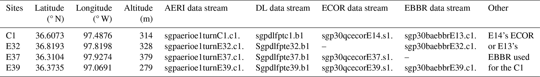
This study utilizes data from the ARM SGP facility, a premier research site established by the U.S. Department of Energy to investigate land-atmosphere interactions in a continental mid-latitude environment (Mather and Voyles, 2013). Located in Oklahoma, USA, the SGP spans a diverse agricultural landscape, making it ideal for studying CBL dynamics under varying meteorological conditions (Mather and Voyles, 2013). We focus on four SGP sites: the central facility (C1) and three extended facilities (E32, E37, E39), selected for their comprehensive measurements of surface fluxes, vertical velocities, and atmospheric profiles. The latitude and longitude coordinates of the four sites are shown in Table 1 (Wulfmeyer and Turner, 2018). The C1 site, located near Lamont, Oklahoma, serves as the primary hub, hosting a suite of instruments including radiosondes, a Doppler lidar (DL), and an Atmospheric Emitted Radiance Interferometer (AERI). The extended sites – E37 and E39 – are equipped with Eddy Correlation (ECOR) systems for surface flux measurements. Additionally, the nearby E14 site (Lamont, Oklahoma; 36.605° N, 97.485° W, 315 m elevation), co-located with C1, which we attribute to C1 for consistency. The E32, E39, and E13 (near C1) sites employ Energy Balance Bowen Ratio (EBBR) technology to measure heat flux.

Table 1 Instruments and datasets used in this study.

The distances between the ARM SGP sites are as follows: ∼ 40 km for C1-E32, ∼ 77 km for C1–E37, ∼ 41 km for C1-E39, ∼ 57 km for E32-E37, ∼ 67 km for E32-E39, and ∼ 77 km for E37-E39. These distances ensure a range of spatial variability in surface and atmospheric conditions, enabling robust evaluation of the model's transferability across sites (Sisterson et al., 2016). The C1 site's DL provides high-resolution vertical velocity and backscatter data, while radiosondes offer 4th-daily temperature and humidity profiles. The AERI at four sites measures downwelling infrared radiance to derive atmospheric stability metrics.

2.2 Data and preprocessing

The dataset comprises multiple variables critical for CBLH estimation, sourced from the ARM SGP sites over the period 2016–2019. The DL used are Halo Photonics Stream Line models (1.5 µ m wavelength), with the C1 site featuring an upgraded Stream Line XR+ model for enhanced signal-to-noise ratio (SNR). These lidars provide a vertical resolution of 30 m and a temporal resolution of 1–3 s, ensuring detailed vertical velocity profiles (Newsom and Krishnamurthy, 2022). The CBLH is calculated using Chu et al. (2022)'s algorithm on ARM DL data, utilizing wavelet analysis to account for turbulence eddy size and gravity wave effects, and applying dynamic thresholds to estimate CBLH from 2-D vertical velocity variance. LTS is derived from AERI observations at C1, calculated as the potential temperature difference between 700 and 1000 hPa (LTS $={\mathit{\theta }}_{\mathrm{700}}-{\mathit{\theta }}_{\mathrm{1000}}$), validated against radiosonde data (Feltz et al., 2003; Wood et al., 2006). Surface fluxes, including SHF and LHF, are obtained from ECOR systems at C1 (via E14), E37, and E39, and from the EBBR system at C1 (via E13), E32, and E39. The ECOR systems use eddy covariance techniques to measure turbulent fluxes, while the EBBR system estimates fluxes via the Bowen ratio method, incorporating net radiation, soil heat flux, and temperature-humidity gradients (Cook, 2018a, b).

Previous studies have shown significant flux discrepancies between ECOR and EBBR beams obtained through different detection techniques, making them non-interchangeable for direct use (Tang et al., 2019; Chu et al., 2026). Data preprocessing involves quality control to remove outliers and missing values, following ARM's standard protocols (e.g., flagging data with unrealistic values or low SNR).

2.3 Machine learning methods

ML algorithms have emerged as powerful tools in atmospheric science, enabling the analysis of complex, non-linear relationships within large datasets to improve predictions of phenomena such as CBLH (Krishnamurthy et al., 2021). ML methods excel at identifying patterns in atmospheric data, enhancing applications like weather forecasting, air quality modeling, and boundary layer parameterization by integrating diverse data sources, including ground-based observations and reanalysis products (Reichstein et al., 2019). Two prominent ML approaches for regression tasks are decision tree-based methods and neural networks, each offering distinct advantages for atmospheric applications (Bauer et al., 2015; de Burgh-Day and Leeuwenburg, 2023).

Decision tree-based methods partition data into hierarchical decision nodes, creating a flowchart-like structure to predict outcomes based on input features. Advanced ensemble techniques, such as random forests and gradient boosting, combine multiple trees to improve accuracy and robustness, making them well-suited for tasks like CBLH estimation (Breiman, 2001; Chen and Guestrin, 2016). Neural networks, conversely, consist of interconnected layers of nodes that learn intricate patterns through backpropagation, excelling in capturing non-linear dynamics in atmospheric datasets, such as turbulence or stability gradients (Goodfellow et al., 2016). Automated ML frameworks streamline model development by optimizing architectures and hyperparameters(Salehin et al., 2024). Prior studies have compared frameworks like AutoKeras (Zhong et al., 2024; Liang et al., 2024), which automates neural network design, and the Tree-based Pipeline Optimization Tool (TPOT), which focuses on tree-based models, finding comparable performance in atmospheric applications (Jin et al., 2019; Olson et al., 2016). Considering computational efficiency and the adaptability of algorithms to diverse datasets, this study does not simultaneously compare the results of various machine learning methods. Instead, it focuses on comparing the outcomes of TPOT and AutoKeras after their automated selection of optimal models. This research employs the automated machine learning frameworks TPOT (version 0.12.2) and AutoKeras (version 1.0.20), integrated within a Python 3.9 environment (Windows 11 OS, Intel^® Core™ i9-10900 CPU @ 2.8 GHz, 32 GB RAM). Development was executed using the spyder-kernels package (version 2.4.4), ensuring robust and reproducible computational workflows.

2.4 Implicit physical constraints

2.4.1 Parameter selection based on thermodynamic equilibrium constraints

Traditional machine learning methods for predicting CBLH typically employ Principal Component Analysis (PCA) or random combinatorial approaches to select input parameters (Liu et al., 2022). While these methods can achieve good predictive performance at specific sites, they lack a physical basis, resulting in poor transferability across different sites and limiting their applicability. To address this issue, this study proposes an innovative approach by incorporating the physical foundation of thermodynamic equilibrium to optimize parameter selection, thereby developing a CBLH prediction model that is transferable across sites. As noted by Stull (1988), although the development of the CBL is influenced by multiple factors, thermodynamic equilibrium is the primary driver of its evolution. Figure 1a depicts the surface heat flux evolution following solar radiation absorption, while Fig. 1b illustrates the heat required for CBL growth, which together determine the CBLH and is used as the theoretical framework to quantify the dynamic evolution of the CBLH in this study. Specifically, the relationship is described by the following integral expression:

$$\begin{array}{}\text{(1)}& \underset{t=\mathrm{0}}{\overset{t_{\mathrm{1}}}{\int }}\overline{w^{\prime }{\mathit{\theta }}_s^{\prime }\left(t\right)}\mathrm{d}t=\underset{\mathit{\theta }={\mathit{\theta }}_{\mathrm{0}}}{\overset{{\mathit{\theta }}_{\mathrm{1}}}{\int }}Z\left(\mathit{\theta }\right)\mathrm{d}\mathit{\theta }.\end{array}$$

Here, $\overline{w^{\prime }{\mathit{\theta }}_s^{\prime }\left(t\right)}$ denotes the time-averaged heat flux (W m⁻²), Z(θ) represents boundary layer height as a function of potential temperature, and θ is potential temperature (K). This formulation reflects the role of surface heat flux and low troposphere stability in driving boundary layer growth, where the left-hand side represents the cumulative contribution of surface heat flux over time, and the right-hand side describes the amount of heat required to produce a well-mixed CBL. Therefore, it provides a solid physical foundation for the model, ensuring that parameter selection not only enhances predictive capability but also maintains physical consistency across different sites (e.g., C1, E32, E37, E39).

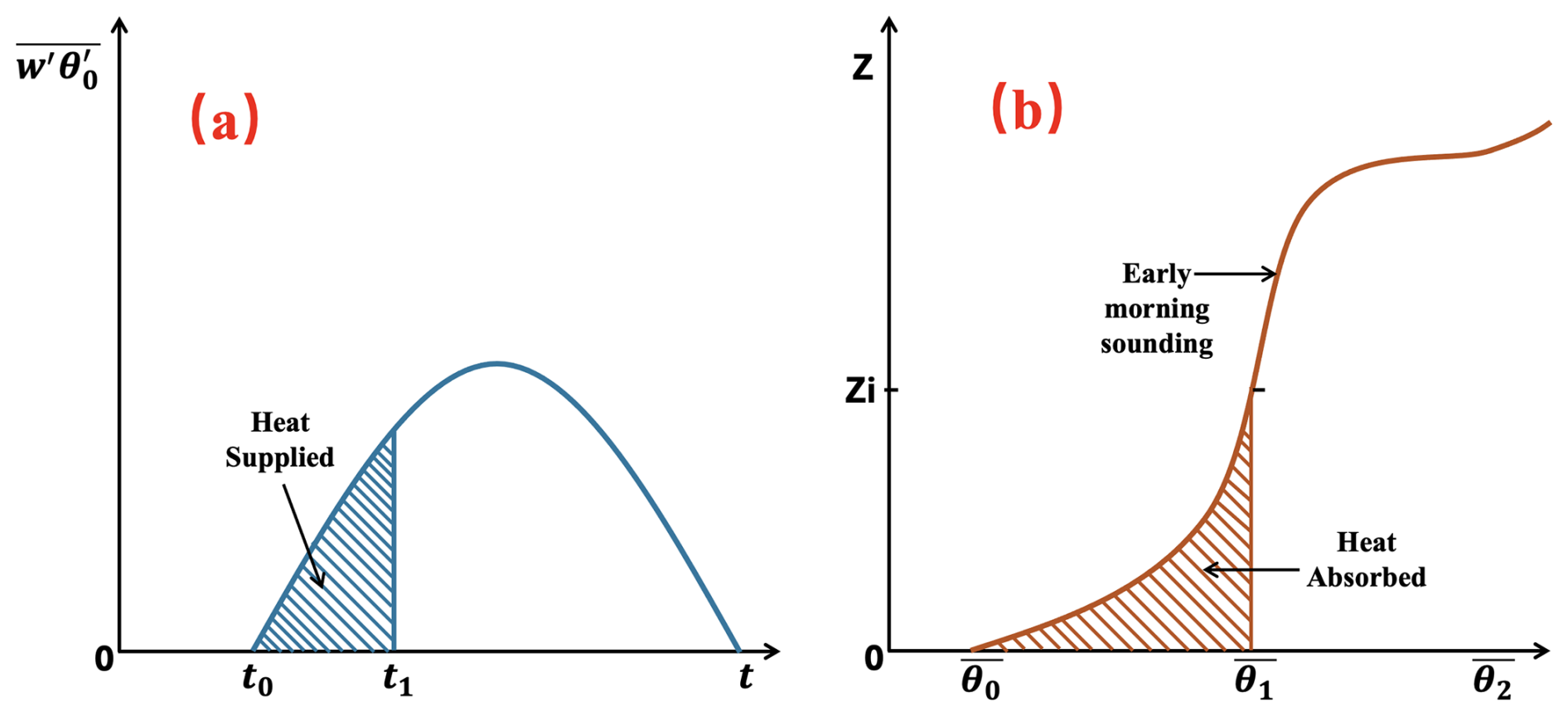
Figure 1 Graphical approach to estimate Convective Boundary Layer Height (CBLH) thermodynamically by equating heat supplied with heat absorbed; Zi is CBLH (adapted from Stull, 1988).

However, Eq. (1) only provides a robust physical constraint during the development from sunrise to the top of the CBL. After reaching the BL top, the entrainment process in the entrainment zone must also be considered. The entrainment process is till poorly understood. Additionally, factors, such as moisture, wind speed, wind direction, and cloud cover, could introduce complex, nonlinear effects on CBL development. Therefore, the direct application of Eq. (1) is not enough to constrain full daily CBL evolution. This study proposes an innovative approach that combines heat flux with LTS as major inputs to achieve implicit physical constraints in ML models.

Surface heat flux and LTS as core inputs ensure the ML model's physical consistency and transferability. The heat flux is further broken down into physical components, including the cumulative sensible heat flux (C_SHF) and latent heat flux (C_LHF) since sunrise, as well as the instantaneous sensible heat flux (I_SHF) and latent heat flux (I_LHF) within a one-hour window, while LTS is taken as an hourly instantaneous value. This parameterization effectively captures diurnal variations in solar radiation, enriching the model with more comprehensive physical information. To address diurnal and seasonal variations in CBLH, the model incorporates sunrise and sunset times along with their corresponding timestamps, defining a normalized temporal parameter,

$$\begin{array}{}\text{(2)}& \begin{array}{rl}\text{SUNPERCENT}& =(\text{TIME}-\text{SUNRISE})/\\ & (\text{SUNSET}-\text{SUNRISE}),\end{array}\end{array}$$

which represents the proportion of the current time relative to the daylight duration. In summary, this study employs physically driven variables for parameter selection – specifically surface heat flux and LTS as core inputs – to ensure the model's physical consistency and transferability. The heat flux is further broken down into physical components, including the cumulative sensible heat flux (C_SHF) and latent heat flux (C_LHF) since sunrise, as well as the instantaneous sensible heat flux (I_SHF) and latent heat flux (I_LHF) within a one-hour window, while LTS is taken as an hourly instantaneous value. This parameterization effectively captures diurnal variations in solar radiation, enriching the model with more comprehensive physical information.

2.4.2 Integrated Diurnal Evolution of the CBL

The current approaches on predicting CBLH using machine learning predominantly focus on discrete, moment-to-moment predictions, often overlooking the integrated diurnal evolution of the CBL as a unified process. For instance, Chu et al. (2025a) employed ML to estimate CBLH over the Southern Great Plains, but this approach centered on individual time steps, neglecting the full diurnal cycle. However, as shown in Fig. 2, the diurnal variation of CBLH across five ARM sites reveals distinct site-specific patterns. The CBLH at each moment evolves continuously from the preceding moment, establishing a dynamic and interconnected developmental trajectory. Treating these moments in isolation disrupts this continuity, failing to capture the underlying evolutionary dynamics. Specifically, the peak CBLH values vary across the sites, and the morning growth and evening decay phases exhibit notable differences, highlighting the critical role of temporal dependencies in boundary layer evolution. While some studies incorporate the CBLH of the previous moment – or CBLH derived from alternative methods, such as sensible heat flux or parcel methods – as an input variable, this approach often overemphasizes the influence of prior CBLH values, thereby overshadowing the contributions of other meteorological drivers. For example, Su et al. (2024) demonstrated that machine learning models relying heavily on CBLH derived from sensible heat flux and parcel methods tend to exhibit excessive dependence on temporal autocorrelation, which diminishes the model's sensitivity to key meteorological factors such as heat flux and atmospheric stability. Consequently, these methods are limited in their ability to comprehensively predict the diurnal variation of CBLH, constraining the scope of their investigations.

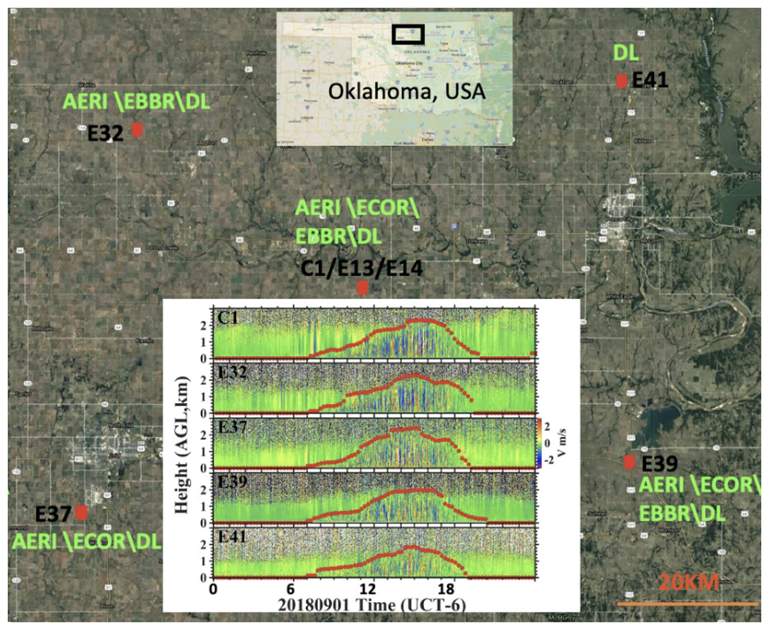
Figure 2 Relative locations of ARM SGP Sites C1, E32, E37, E39, and E41. Top inset: geographic position of SGP sites in Oklahoma; bottom inset: diurnal variation of CBLH observed by Doppler lidar across the five sites on 1 September 2018 (background: © Google Maps).

To address these shortcomings, this study adopts the CBLH across the entire diurnal cycle as the training target for the machine learning model, treating the CBL evolution as a continuous and interconnected process. This holistic approach enables the model to comprehensively capture the dynamic evolution of the boundary layer, from the gradual rise of the CBLH after sunrise, through its midday peak accompanied by oscillations, to the rapid decay observed after sunset. By integrating the complete developmental trajectory, the model not only better represents the interconnected dynamics of the CBL but also accounts for the complex interplay of meteorological drivers that govern its evolution. For instance, the morning growth phase is heavily influenced by surface heating and turbulent mixing, while the midday peak often reflects a balance between entrainment processes at the boundary layer top and surface-driven convection. The evening decay phase, on the other hand, is modulated by radiative cooling and the cessation of surface heat fluxes, which vary significantly across different sites due to local land surface characteristics and atmospheric conditions. To enhance the model's predictive capability, we incorporate time-dependent variables that reflect the diurnal cycle's progression. This approach mitigates the overreliance on prior CBLH values by ensuring that the model learns the underlying physical relationships between CBLH and its meteorological drivers, rather than simply exploiting temporal autocorrelation. As a result, the model is expected to improve the accuracy of CBLH predictions across the diurnal cycle, offering a more comprehensive understanding of boundary layer dynamics.

2.5 Auto-ML model for CBLH

We prepared the relevant input parameters and employed the following methodology to enable the machine learning approach to uncover the complex physical mechanisms underlying the physical parameters. After the compilation environment was set up and the data was prepared, the specific model application process (Fig. 3) is as follows:

1. Data Collection and Pre-processing. Based on the content of Sect. 2.1 and 2.2, we prepare the data for each timestamp of the day, including C_SHF, C_LHF, I_SHF, I_LHF, LTS, TIME, SUNRISE, SUNSET, SUNPERCENT, and CBLH. The SUNRISE and SUNSET represent the sunrise and sunset times calculated based on the latitude and longitude coordinates of the site. To simplify the dataset, we aggregate the data from 06:00 to 21:00 (UTC−6), covering a 15 h period, as a single daily dataset. Although daily SUNRISE and SUNSET values are constant, for comparison consistency, we expanded their dimensions to match the time dimension of other parameters (15 h in this study). Thus, all input and output parameters have a uniform dimension of 15. The CBLH for the entire day is designated as the target variable for output, while the other parameters serve as input variables. We randomly split all the data into 70 % for training and 30 % for testing by date. The subfigure in Fig. 3 that depicts the ARM site, included in the Data Collection section, is adapted from Wulfmeyer and Tang (2018).

2. Use AutoML to find the Best Train Model. Using the training dataset, we employ TPOT and AutoKeras to derive their respective optimal algorithms or hyperparameters. By comparing the R² and Mean MAE metrics, we select the model that performs best in both MAE and R² as the optimal model, which is then designated as the candidate best model for further evaluation and application.

3. Use the Best Model with training Data for Training. The best model is trained on the training dataset and saved for later use, ensuring optimal performance for future applications.

4. One-Day CBLH Prediction. Use the trained model to predict CBLH for a single day.

Figure 3's flowchart outlines the algorithm proposed in this study (termed the Auto-ML algorithm). Its core principles are: (1) utilizing thermodynamical variables as input parameters with implicit physical constraints; (2) incorporating the complete CBL development cycle as unified input, with corresponding CBLH as output; and (2) employing TPOT and AutoKeras models to automatically select the optimal machine learning algorithm. This approach enables the model to capture the entire CBL development process, enhancing prediction accuracy and representation of CBL dynamics.

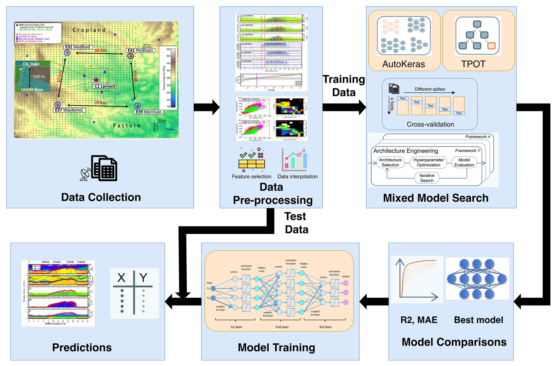
Figure 3 The Auto-ML workflow of CBLH.

3 Results

To validate the effectiveness of the Auto-ML framework, we first conducted tests using data from the C1 site spanning 2016 to 2019, presenting the results for ECOR and EBBR heat flux, respectively. Subsequently, the algorithm was evaluated by appling to other sites. Next, we compared the performance of the optimal TPOT and AutoKeras algorithms for summer (JJA) and further evaluated the advantages and limitations of different methods by computing SHAP (Shapley Additive exPlanations) values. Furthermore, we analyzed the variations in Auto-ML's relative importance across seasons. Finally, we compared the performance of models trained on multi-site data and tested on site-specific data.

3.1 Application of the Auto-ML to the ARM SGP C1 Site

The Auto-ML algorithm demonstrates robust performance in predicting CBLH when using ECOR flux dataset. The selected machine learning framework is the ExtraTreesRegressor architecture chosen by TPOT. The scatter predicted CBLH in Fig. 4a demonstrates a strong linear correlation (R²=0.85) between predicted and observed CBLH across the annual dataset, suggesting that the Auto ML model effectively captures the general trends of CBL evolution (Fig. 4a). However, the MAE of 0.21 km highlights a non-negligible systematic bias, potentially linked to specific meteorological conditions or seasonal variations not fully resolved by the model. Notably, the density of point clusters around the 1:1 line in the lower CBLH range (0–1.5 km), while deviations increase slightly at higher CBLH values (> 2 km), possibly indicating reduced model sensitivity to extreme events (e.g., intense convective days).

The diurnal variability between predicted and observed CBLH also shows good agreement (Fig. 4b). The predicted CBLH closely tracks observed values during the morning development phase (07:30–13:30 UTC−6), with overlapping interquartile ranges (IQR) from ∼ 0.3 to ∼ 0.8 km, reflecting reliable performance during periods of rapid boundary layer growth driven by surface heating and turbulent mixing. However, a significant divergence emerges in the afternoon (15:30–17:30 UTC−6), where the predicted mean CBLH underestimates observations by ∼ 0.1 km. This discrepancy coincides with the typical peak phase of the CBL, characterized by weakening turbulence, entrainment processes at the CBL top, and increasing influence of subsidence or advection.

The afternoon underestimation may stem from the algorithm's limited ability to resolve complex interactions during the CBL peak phase. During midday, solar radiation maximizes surface heat flux, driving vigorous turbulent eddies that homogenize the CBL, making CBLH prediction relatively straightforward. By late afternoon, surface heating diminishes, turbulence decays, and the entrainment zone at the CBL top becomes dynamically significant. Entrainment of free-tropospheric air into the CBL can temporarily elevate the observed CBLH, a process that may not be easily captured in the Auto ML model due to the inputs lacking information for characterizing entrainment. Additionally, the advection of air masses with different thermodynamic properties (e.g., moisture or temperature gradients) could introduce spatial heterogeneity, further challenging the algorithm's generalizability during transitional periods.

Moreover, the model's training data might underrepresent late-afternoon scenarios, where PBL dynamics are influenced by mesoscale phenomena (e.g., cloud cover or topographic effects). For instance, enhanced subsidence or cloud shading at 15:30–17:30 (UTC−6) could suppress turbulent mixing, leading to a shallower predicted CBLH compared to observations.

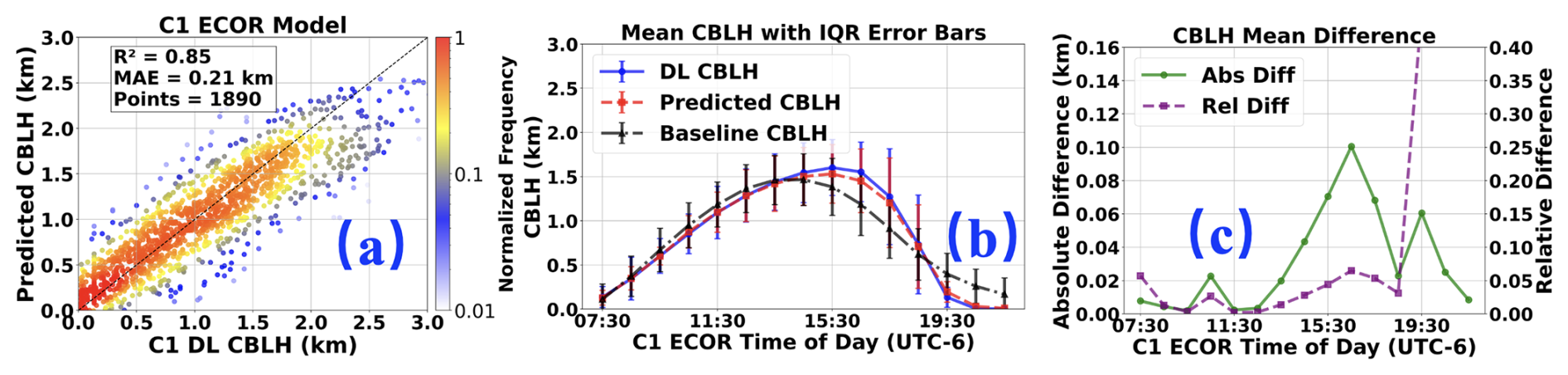
Figure 4 Results of Auto ML model with ECOR dataset for predicting CBLH: (a) Comparison of all test data, (b) Diurnal variation average with IQR (interquartile range), (c) Diurnal variation of absolute and relative difference between DL CBLH and predicted CBLH.

To evaluate the performance of the AutoML algorithm, Linear Regression was used as a competitive baseline. Results at site C1 show that the AutoML model significantly outperformed Linear Regression, which yielded an R² of 0.69 and an MAE of 0.32 km compared to the AutoML's R² of 0.85 and MAE of 0.21 km. Notably, the performance discrepancy reached over 0.5 km during the afternoon and pre-sunset hours (Fig. 4b; see Text S3 and Fig. S1 in the Supplement for further details). To confirm its applicability beyond the ECOR heat flux dataset at C1 site, we compared its performance on the EBBR heat flux dataset. The EBBR can accurately predict the CBLH, comparable to the predictions of the ECOR (see Text S4 and Fig. S2).

A comparison of Fig. 4c reveals that the discrepancies between the predicted values and the DL observations are primarily evident at the PBL top (∼ 15:30 UTC−6) and during the dissipation phase (∼ 19:30 UTC−6). Specifically, at the CBL top (∼ 15:30 UTC−6), the predicted values are generally lower than the DL observations, whereas during the dissipation phase (∼ 19:30 UTC−6), the predicted values tend to exceed the observed values.

3.2 Effectiveness of the Auto-ML Across Multiple Sites

The Auto-ML algorithm demonstrates notable adaptability beyond the C1 site, highlighting its potential for broader application across multiple observation sites. To evaluate this, we tested an Auto-ML model trained on ECOR heat flux data at the C1 site (E14 site) for its performance at the E37 and E39 sites. Similarly, an Auto-ML model trained on EBBR heat flux data at the C1 site (E13 site) was assessed for its performance at the E32 and E39 sites.

The Auto-ML model trained at the C1 site with ECOR data exhibits strong performance at the E37 and E39 sites, achieving R² values of 0.79 and 0.81, and MAE values of 0.22 and 0.21 km, respectively (Fig. 5a and c). However, as observed in Fig. 5b and d, the model's performance varies across different time periods at these sites. Specifically, Fig. 5b shows that at the E37 site, the model predictions align well with observations during the CBLH dissipation phase (15:30–21:30 UTC−6). However, during the initial development phase (07:30–14:30 UTC−6), a significant discrepancy is observed, with predicted values consistently higher than the DL observations. Notably, no similar discrepancy is evident in Fig. 4b, suggesting that additional factors other than heat fluxes and LTS impact CBL development at the C1 and E37 sites during the initial phase, while the differences diminish after reaching the boundary layer top. A similar discrepancy (see Fig. 5d) is also observed at the E39 site during the initial phase (09:30–11:30 UTC−6).

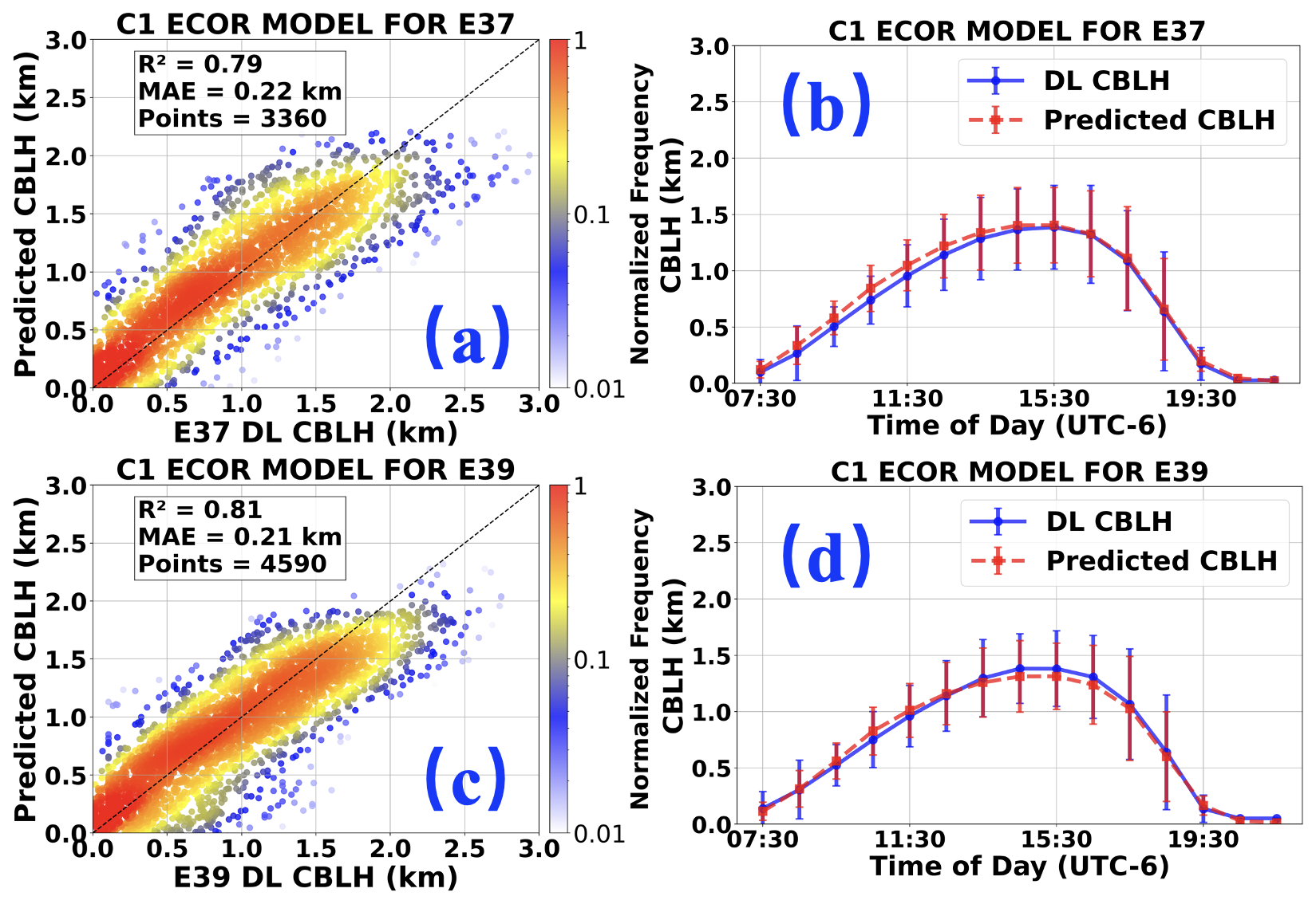
Figure 5 C1 ECOR model for E37 and E39 sites; (a) and (c) represent the R² and MAE for E37 and E39 respectively; (b) and (d) show the MEAN CBLH with IQR for E37 and E39 respectively.

The above analysis indicates that while the Auto-ML model trained at the C1 site performs well at the E37 and E39 sites, its performance varies across different time periods, reflecting both similarities and differences in behavior at these sites. This highlights the spatial variability between sites. Furthermore, the differences between the C1 and E39 sites are smaller than those between the C1 and E37 sites, which aligns with their relative distances (41 km vs. 77 km).

We used the Linear Regression algorithm as a baseline for comparison, with results indicating that the AutoML-derived algorithm outperforms Linear Regression across other sites (see Text S5 and Fig. S3). To demonstrate its applicability beyond the ECOR heat flux dataset, we compared its performance using the EBBR heat flux dataset. The EBBR can also accurately predict the CBLH, comparable to the predictions of the ECOR (see Text S6 and Fig. S4 for details).

The Auto-ML algorithm demonstrates significant adaptability beyond the C1 site, underscoring its potential for wider application across multiple observational stations (Figs. 5 and S4). Although the C1 ECOR model shows inconsistent performance across sites, it accurately predicts CBLH during daytime at all three sites (C1, E37, E39) with an absolute error < 0.10 km (see Text S5 and Fig. S5 for detailed discussion). The Auto-ML model trained at the C1 site performs effectively at the E37 and E39 sites, while models trained at the E37 and E39 sites also exhibit robust performance at the C1 site, achieving R² values of approximately 0.80–0.85 and MAE values ranging from 0.19 to 0.23 km (figures not shown in this study).

3.3 The relationship between Auto-ML model performance and the spatial separation between sites

Section 3.2 demonstrates the cross-site applicability of the Auto-ML algorithm. To further investigate the relationship between Auto-ML performance and the spatial separation between sites, we selected data from the C1 site (E14 and E13 sites with ECOR and EBBR data, respectively) and the E39 site, training separate models using both datasets. These models were then applied to other sites with similar heat flux characteristics to assess the correlation between performances and inter-site distances.

The predictive performance of the Auto-ML algorithm exhibits a clear but now negative correlation with the spatial separation between observational sites (Fig. 6). For instance, as shown by the solid red and dashed lines in Fig. 6, the model trained on ECOR data from the C1 site performs robustly at its primary site (R²=0.85, MAE = 0.20 km), but its accuracy decreases at the E39 site 41 km away (R²=0.80, MAE = 0.21 km) and further declines at the E37 site 77 km away (R² = 0.80, MAE = 0.21 km). A similar decreasing performance with site distance is observed for the model trained on ECOR data from the E39 site.

Despite this overall trend of performance decline with distance, notable irregularities are observed. For example, the model trained on EBBR data from the C1 site performs best at its primary site (R²=0.83, MAE = 0.21 km), with a slight decrease in accuracy at the E39 site 41 km to the southeast (R² = 0.80, MAE = 0.20 km), but a more significant decline at the E32 site 40 km to the northwest (R²=0.72, MAE = 0.27 km). Likewise, the model trained on EBBR data from the E39 site excels at its primary site (R²=0.80, MAE = 0.22 km), maintains comparable performance at the C1 site 41 km to the southeast (R² = 0.81, MAE = 0.23 km), but shows a substantial drop at the E32 site 67 km to the northwest (R² = 0.76, MAE = 0.26 km).

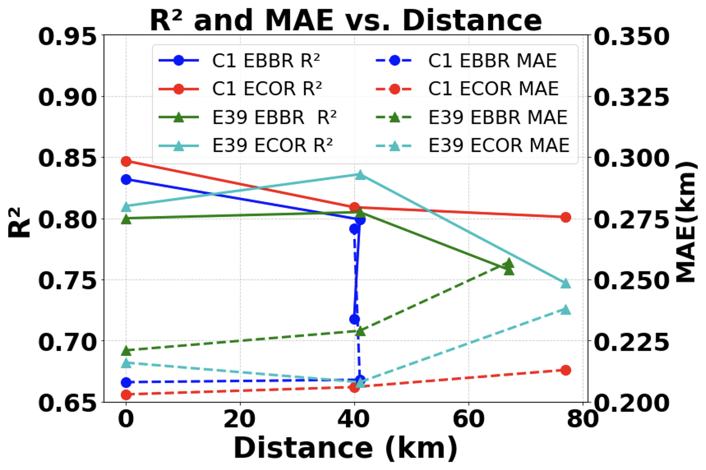
Figure 6 Relationship between Auto-ML model effectiveness and distance evaluated by applying the model trained at one site to other sites.

The sharp performance differences between the E32 and E39 sites with the model trained on C1 EBBR data could be caused by the representativeness of surface flux measurements. ARM's ECOR systems are typically surrounded by winter wheat fields or farmland, whereas EBBR systems are primarily deployed in pastures. The performance drop at E32 may stem from vegetation differences and measurement principles. E32's pasture dominated EBBR data, prone to overestimating latent heat flux, contrasts with the winter wheat fields around C1 and E39, likely measured by ECOR, which directly captures turbulent fluxes. These discrepancies in surface heat flux inputs challenge the model's generalization, particularly at E32, where site-specific factors like soil moisture or EBBR measurement errors near sunrise/sunset may further degrade performance.

This analysis reveals that the predictive performance of the Auto-ML algorithm exhibits a clear negative correlation with spatial separation between sites, accompanied by spatial heterogeneity. These irregularities align with theoretical expectations: local factors such as terrain variations (e.g., changes in elevation or surface roughness), land use differences (e.g., urban vs. rural settings), and microclimate effects (e.g., humidity or temperature gradients) disrupt the coherence of CBL dynamics with increasing distance. These site-specific perturbations limit the algorithm's generalizability across diverse regions.

3.4 Comparison of Performances of two ML methods for summer at the C1 site

Here, the performance of two high-performing machine learning models – an ExtraTreesRegressor from TPOT and a neural network from AutoKeras, is compared with the June–July–August (JJA) season selected due to its higher variability in deep learning-derived CBLH and larger data volume, thereby enhancing the reliability of the results. Both models are trained on the same dataset. The primary advantage of the ExtraTreesRegressor is its built-in resistance to overfitting, achieved through randomized feature selection and split point selection. As a result, the model performs well on high-dimensional data and noisy datasets and shows strong resilience to outliers. However, it is not suitable for small-sample datasets. The best-performing model selected by AutoKeras is a neural network with 10 836 parameters, implemented using the Functional API. It comprises an input layer for 9-dimensional features, preprocessing layers for multi-category encoding and normalization (19 non-trainable parameters), two dense hidden layers with 256 and 32 units respectively (ReLU activation, 10 817 trainable parameters), and a regression output layer. The architecture leverages AutoKeras's automated feature engineering through integrated preprocessing, while its two-layer structure maintains moderate complexity. The parameter distribution (256 to 32 units) indicates a progressive reduction in feature dimensionality, supporting effective feature extraction for the regression task. The ExtraTreesRegressor selected by TPOT is configured with key hyperparameters that optimize its performance: n_estimators: 100, defining 100 trees for robust ensemble learning; max_depth: None, allowing unrestricted tree depth to capture complex patterns; min_samples_split: 6 and min_samples_leaf: 6, setting minimum samples for splits and leaves to control overfitting; and max_features: 1.0, considering all features per split for comprehensive feature utilization. These settings enhance its resistance to overfitting and suitability for high-dimensional, noisy datasets.

3.4.1 SHAP Computation Methods: Tree-Based vs. Gradient Approaches

To compare the relative importance of features between the two methods, SHAP values (Cunha and Barbosa, 2024) for the ExtraTreesRegressor are computed directly using the TreeExplainer, which leverages the tree structure (split paths and leaf node values). In contrast, the AutoKeras neural network employs the GradientExplainer, a gradient-based method, to estimate SHAP values. SHAP values are calculated by treating each day as a whole, rather than individual time segments within a day. Their summer (JJA) performance, shown in Fig. 7, reveals similar R² and MAE values: ExtraTreesRegressor (0.86, 0.22 km) versus neural networks (0.84, 0.25 km), as depicted in Fig. 7a (ExtraTreesRegressor) and Fig. 7e (neural networks). These consistent metrics highlight the robustness of both approaches in capturing CBLH. However, despite their similarity in overall performance, the two models diverge significantly (SHAP method) in their assessment of feature importance. In Fig. 7c, ExtraTreesRegressor assigns a notably higher importance to LTS (∼ 0.23); attributes nearly equal importance to I_SHF, I_LHF, TIME, and SUNPERCENT each hovering around 0.15, indicating a clear prioritization of LTS in its decision-making process. In contrast, the neural network, as shown in Fig. 7g, assigns a notably higher importance to I-LHF (∼ 0.28); attributes nearly equal importance to C_SHF and I_SHF, each hovering around 0.2. The different machine learning models can achieve comparable accuracy by using varied nonlinear combinations of predictors. In such scenarios, the physical interpretation of these models becomes challenging or may lack sufficient reliability. Figure 7b and d show that the diurnal variations predicted by the AutoKeras neural network and the TPOT ExtraTreesRegressor are generally comparable. However, Fig. 7f reveals that the neural network predicts lower CBLH values than the ExtraTreesRegressor (Fig. 7b) between 07:30–11:30 and around 19:30 UTC−6. Despite this, the neural network exhibits inferior performance, with lower R² and higher MAE compared to the ExtraTreesRegressor.

A comparison of Fig. 7g–h (neural network) with Fig. 7c–d (ExtraTreesRegressor) highlights distinct differences in feature contributions. For the neural network, the SHAP values and relative importance of TIME, SUNRISE, and SUNSET are zero, whereas SUNPERCENT retains a non-zero SHAP value. This suggests that the neural network effectively captures the information encoded in Eq. (5), prioritizing SUNPERCENT as the primary contributor to CBLH predictions. In contrast, the ExtraTreesRegressor assigns reduced but non-zero relative importance to SUNRISE and SUNSET, indicating a broader distribution of feature contributions.

These differences likely stem from the distinct SHAP explainers used for each model. The ExtraTreesRegressor employs the TreeExplainer, which leverages the tree structure (split paths and leaf node values) to compute SHAP values directly, without requiring a background dataset. Conversely, the neural network uses the GradientExplainer, a local explanation method that relies on a background dataset (100 samples in this study) and computes SHAP values based on gradients near specific input points. When the local gradient for features such as TIME, SUNRISE, and SUNSET approaches zero, this reflects their negligible impact on the model's local decision boundary, resulting in corresponding SHAP values of zero. This explains the neural network's tendency to assign zero importance to these features, while the ExtraTreesRegressor's global approach captures their residual contributions.

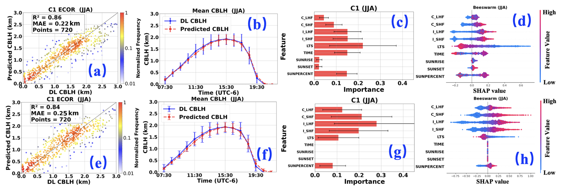
Figure 7 Performance comparison of two machine learning frameworks during summer (JJA) (a–d) ExtraTreesRegressor (a) Comparison of observed and predicted CBLH; (b) Diurnal evolution of mean observed and predicted CBLH; (c) SHAP-derived feature importance; (d) Beeswarm plot of SHAP values; (e–h) Corresponding panels for Neural Network: (e) observed vs. predicted CBLH; (f) diurnal variations; (g) SHAP-derived feature importance; (h) Beeswarm plot of SHAP values.

3.4.2 Comparative Analysis of SHAP Value Estimation Methods for AutoKeras Neural Networks

To validate the reliability of SHAP values and assess differences across computation methods, we compare the results of alternative SHAP explainers with those shown in Fig. 7g–h. The GradientExplainer, used for the AutoKeras neural network, approximates SHAP values by computing gradients of input features relative to model outputs, relying on a background dataset (100 samples in this study) to estimate feature contributions. The choice of background dataset can influence results, as GradientExplainer assumes local differentiability and quantifies feature importance based on gradient information. Consequently, features with near-zero gradients (e.g., those with minimal local influence near the background dataset) may yield zero SHAP values.

To mitigate this limitation, two additional explainers were employed: (1) KernelExplainer, a model-agnostic method that estimates SHAP values through sampling and weighted regression, suitable for any model. By sampling the global feature space, it captures non-local or nonlinear contributions, potentially yielding non-zero SHAP values even when local gradients are zero. However, KernelExplainer still requires a background dataset. (2) ExactExplainer, which does not require an explicit background dataset but uses a masking strategy, typically shap.maskers.Independent, to implicitly define the background distribution based on the data itself (Ponce-Bobadilla et al., 2024). By precisely computing Shapley values for all feature combinations, ExactExplainer provides the theoretically most accurate SHAP estimates, though it is computationally intensive.

Table 2 Performance comparison of various SHAP value calculation methods on feature importance.

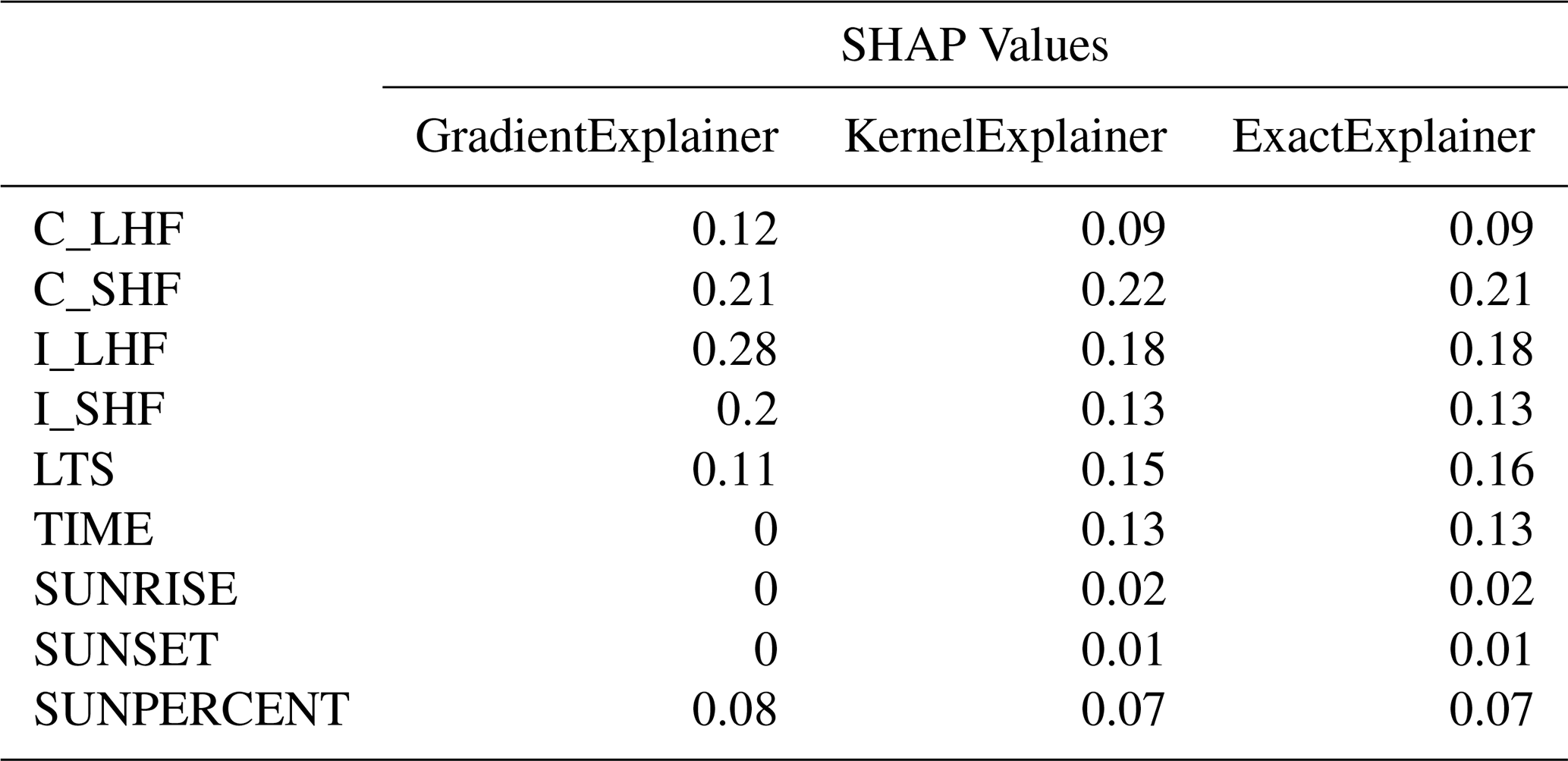
Table 2 summarizes the performance of different SHAP explainers. The GradientExplainer assigns zero SHAP values to input features with low influence, resulting in larger errors, but it offers high computational efficiency and requires fewer resources. In contrast, the ExactExplainer provides more reliable results but incurs high computational complexity, making it resource-intensive. For scenarios with limited computational resources and a need for high-accuracy SHAP values, the KernelExplainer is recommended as a balanced alternative. Notably, for features with lower relative importance, such as TIME, SUNRISE, and SUNSET, the ExactExplainer and KernelExplainer yield nearly identical results, with minor differences (approximately 0.01) observed for C_SHF and LTS.

Based on these findings, the SHAP value computation strategy in this study is as follows: For the TPOT-selected model (ExtraTreesRegressor), the TreeExplainer is used, leveraging its efficiency for tree-based models. For the AutoKeras neural network, the ExactExplainer is employed to compute SHAP values when computational resources are sufficient; however, the KernelExplainer is preferred when resources are limited.

3.5 Seasonal comparative analysis of Auto-ML's performance

3.5.1 Seasonal comparative analysis of Auto-ML's comprehensive performance

The performance of Auto-ML varies across different sites and seasons. As shown in Fig. 8, after training with multi-year ECOR data at C1 sites, the model's performance is evaluated across four seasons. Figure 8a1–8a4 illustrate that autumn (SON) achieves the highest overall R² (0.860) but ranks second in MAE (0.178 km). Winter (DJF) exhibits the lowest MAE (0.173 km) but the poorest R² (0.736). Summer (JJA) records the highest overall CBLH with strong performance (R²: 0.855, MAE: 0.221 km). Spring (MAM) yields an R² of 0.768 and an MAE of 0.239 km. Given the higher CBLH in summer and lower CBLH in winter, Auto-ML performs best overall in autumn. As illustrated in Fig. 8c2 and 8c4, the absolute differences for summer and winter are all below 0.14 km. However, the relative differences in summer are less than 0.1 except for the 19:30 UTC−6 (∼ 0.3); in contrast, the relative differences between morning and evening in winter exceed 0.5. Consequently, Auto-ML exhibits the best overall performance in summer.

3.5.2 Season-wise comparison of hourly averaged AutoML performance

However, when considering diurnal variations across seasons, summer (JJA) appears to perform best. As shown in Fig. 8b1–8b4, predictions for spring (MAM) and autumn (SON) near the CBL top phase are approximately 0.1 km lower than DL observations. In winter (DJF), due to lower overall CBLH, predictions are about 0.05 km below observations. In contrast, summer (JJA) shows no significant discrepancy near the CBL top (12:30–14:30 UTC−6), with predictions only slightly lower (∼ 0.05 km) around 11:30 UTC−6. Potential reasons include: (1) a larger number of summer data points, leading Auto-ML model weighted more to summer conditions, and (2) distinct entrainment processes in summer compared to other seasons.

The entrainment process at the top of the atmospheric boundary layer exhibits a dual influence on boundary layer development. When warm, dry air is entrained into the boundary layer, it enhances turbulent mixing and promotes vertical growth (Angevine et al., 1998). Conversely, if a strong inversion layer exists aloft, entrainment can suppress convection by dissipating turbulent kinetic energy and reducing upward heat flux (Lenschow et al., 2012). The entrainment rate ω_e, defined as the volume flux of air drawn from the free atmosphere into the mixing layer per unit time at the boundary layer top, follows a modified form of the classical entrainment parameterization (Lilly, 1968; Deardorff, 1979; Stull, 1988; Sullivan et al., 1998):

$$\begin{array}{}\text{(3)}& {\mathit{\omega }}_{\mathrm{e}}=A{\displaystyle \frac{{\mathit{\omega }}_{\ast }^{\mathrm{3}}}{h\mathrm{\Delta }{\mathit{\theta }}_{\mathrm{v}}}}\end{array}$$

where, the entrainment efficiency coefficient A is around 0.2 (Beare et al., 2006; Cuxart et al., 2006; Pino et al., 2003); h is CBLH, ω_∗ is convective velocity scale(Deardorff, 1979); Δθ_v is virtual potential temperature jump (virtual potential temperature at the bottom of the inversion layer – average virtual potential temperature of the mixing layer). Equation (3) indicates that deeper boundary layers (larger h) exhibit weaker entrainment due to diminished turbulent energy (Beare, 2008). Additionally, when cloud fraction exceeds ∼ 60 %, the boundary layer growth rate declines by over 50 %, as cloud shading suppresses surface-driven turbulence (Zhang et al., 2020).

In humid summer conditions, high specific humidity (> 18–20 g kg⁻¹) further inhibits boundary layer growth through multiple pathways: (a) increased cloudiness reduces surface solar heating (Luo et al., 2024), (b) precipitation depletes convective available potential energy (Hohenegger and Stevens, 2013), and (c) evaporative cooling enhances stability (Zhang, 2003). Observational studies confirm that tropical moist boundary layers are 30 %–40 % shallower than their arid counterparts (von Engeln and Teixeira, 2013), highlighting moisture's threshold-like suppression effect.

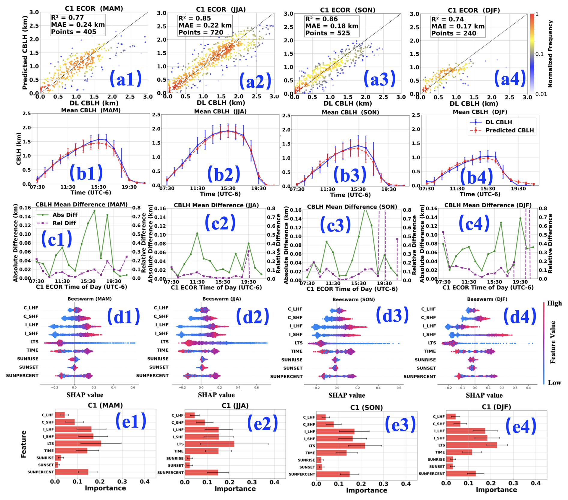
Figure 8 Seasonal performance of the C1 ECOR model. The four columns represent the four seasons: spring (MAM), summer (JJA), autumn (SON), and winter (DJF); (a) Comparison of observed and predicted CBLH; (b) Diurnal evolution of mean observed and predicted CBLH; (c) Diurnal evolution of Absolute difference and relative difference between observed and predicted mean CBLHs; (d) Beeswarm plot of SHAP values for four-season analysis; (e) SHAP-derived feature importance for four-season analysis.

The AutoML model developed in this study predicts CBLH across all seasons, with mean differences between DL-derived and predicted CBLH consistently within 0.2 km. Notably, in summer (JJA, Fig. 8c2), the mean difference is less than 0.1 km, demonstrating the model's robust performance.

Despite the close agreement in mean values, the IQR of DL CBLH is consistently wider than that of predicted CBLH across all seasons, with the most pronounced difference in JJA (Fig. 8b2). This suggests greater variability in boundary layer development, likely driven by meteorological factors such as wind-driven advection and entrainment processes, which are not fully captured by the thermodynamic parameters (e.g., surface heat flux and LTS) used in the model. For instance, at 11:30 UTC−6, the IQR of DL CBLH (∼ 600 m) is approximately four times larger than that of predicted CBLH (∼ 150 m). In summer, the model may not account for perturbations like upstream air mass advection or enhanced entrainment due to intense convective activity, contributing to the larger IQR in DL CBLH.

In winter (DJF, Fig. 8a4), the model captures the CBL evolution well but exhibits reduced performance (R² = 0.736), likely due to challenges in accurately estimating surface fluxes under cold, frozen surface conditions. The smaller winter sample size (240 points) compared to summer (720 points) further contributes to higher uncertainty. The IQR during winter is generally smaller than during summer. For instance, around 11:30 UTC−6, the IQR of the DL-derived CBLH is approximately 300 m, while that of the predicted CBLH is less than 100 m. This is consistent with the winter CBLH (top ∼ 1 km) being lower than the summer CBLH (top ∼ 2 km).

As shown in Fig. 8c, the absolute differences in mean CBLH are peaking at noon, whereas the relative differences are more pronounced in the morning and evening. For example, although the absolute difference between observed and predicted CBLH from 11:30 to 15:30 UTC−6 across the four seasons can reach 0.1–0.17 km, the relative difference between observed and predicted CBLH during this period remains below 0.1. In contrast, the relative difference between observed and predicted CBLH in the morning and evening is generally less than 0.12 km, but the relative difference can exceed 0.5 km in autumn and winter.

These seasonal differences in variability about mean CBLH difference and the IQR difference are important findings, as they are not explicitly documented in prior literature. We hypothesize that the complex interactions involving advection and entrainment, which the current model does not fully resolve, contribute differently among seasons to CBL development. To improve model performance, future work should incorporate additional parameters, such as entrainment rates and wind profiles, to better capture these processes and improve CBLH variability predictions.

3.5.3 Visualizing SHAP dependencies with Beeswarm plots

Analysis of Fig. 8d1–d4 reveals the relationships between various variables and CBLH. Firstly, the heat flux components (C_SHF, C_LHF, I_SHF, I_LHF) exhibit a predominantly positive correlation with CBLH, indicating that stronger heat flux corresponds to greater CBLH. Conversely, LTS shows a negative correlation with CBLH, suggesting that higher LTS values are associated with reduced CBLH. Time and SUNPERCENT display a biphasic relationship with CBLH: a positive correlation is observed during the pre-peak phase, where CBLH increases with time, while a negative correlation emerges post-peak as CBLH decreases with time. This behavior is consistent with CBL dynamics. Additionally, SUNRISE exhibits a weak negative correlation with CBLH, implying that later sunrise times correspond to lower CBLH, whereas earlier sunrise times are linked to higher CBLH. Similarly, later sunset times are associated with higher CBLH, and earlier sunset times with lower CBLH. These patterns align well with the established development processes of the atmospheric boundary layer. Since SUNPERCENT integrates the effects of time, sunrise, and sunset, its relationship with CBLH closely mirrors that of time.

While the general relationships between input parameters and CBLH are outlined above, seasonal variations are notable. For instance, LTS consistently exhibits a negative correlation with CBLH in spring (MAM), autumn (SON), and winter (DJF). However, in summer, certain data points show a positive correlation, suggesting that under specific complex meteorological conditions in summer, factors beyond LTS dominate CBLH development, further highlighting the complexity of summer CBL dynamics. Additionally, I_LHF displays a positive correlation with CBLH across spring, summer, and autumn, but a negative correlation in winter, despite most corresponding SHAP values exceeding −0.1, creating a stark contrast with the other seasons. A similar, though less pronounced, trend is observed with C_SHF in winter. This phenomenon may be attributed to the dominance of northerly monsoon winds in winter, exacerbating cold, dry conditions. An increase in I_LHF could reduce I_SHF, potentially suppressing turbulence generation. In winter, both SUNRISE and SUNSET exhibit a negative correlation with CBLH, indicating that the overall CBLH remains low during this season. The specific mechanisms underlying these phenomena require further investigation.

3.5.4 Relative importance of input parameters in Auto-ML model

The relative importance of different parameters across the four seasons exhibits a consistent pattern (Fig. 8e1–e4). LTS ranks highest (0.2–0.25), as it determines the energy required for CBLH growth. Next are the instantaneous heat flux components (I_SHF: 0.15–0.18 and I_LHF: 0.15–0.18), indicating that current heat flux plays a critical role in sustaining CBLH. Following these are TIME (0.12–0.15) and SUNPERCENT (0.12–0.15), which collectively govern the diurnal variation in boundary layer development; a positive correlation is observed before CBLH peaks (typically when SUNPERCENT is around 0.5), transitioning to a negative correlation post-peak. Subsequently, C_SHF (0.06–0.09) exceeds C_LHF (∼ 0.05) in influence. The least impactful factors are SUNRISE (∼ 0.02) and SUNSET (0.01–0.02). These relative importance values are consistent with the discussion in Sect. 3.5.3.

However, minor seasonal variations in the relative importance of these parameters are observed. For instance, in summer, LTS reaches a relative importance of 0.22, but its error bar extends to 0.3, suggesting that while LTS temporarily dominates CBLH development, its influence is significantly modulated by other conditions, underscoring the complexity of summer boundary layer dynamics. In contrast, during winter, LTS maintains a relative importance of approximately 0.23 with an error bar of only 0.1, indicating its dominant and stable role in governing winter boundary layer development.

3.6 Comparative analysis of multi-site training with site-specific testing

Previous analyses employed Auto-ML models trained separately for individual sites. To investigate potential performance improvements, we conducted experiments using combined multi-site training followed by site-specific testing while controlling for cross-heat-flux interference. Two independent test groups were evaluated: the ECOR cluster (C1, E37, E39) and the EBBR cluster (C1, E32, E39), with comparative results presented in Table 3. Figure 9 further illustrates the CBLH diurnal variation patterns to enhance temporal resolution analysis.

Table 3 The performance of predictive models and feature importance results of multi-site training with site-specific testing.

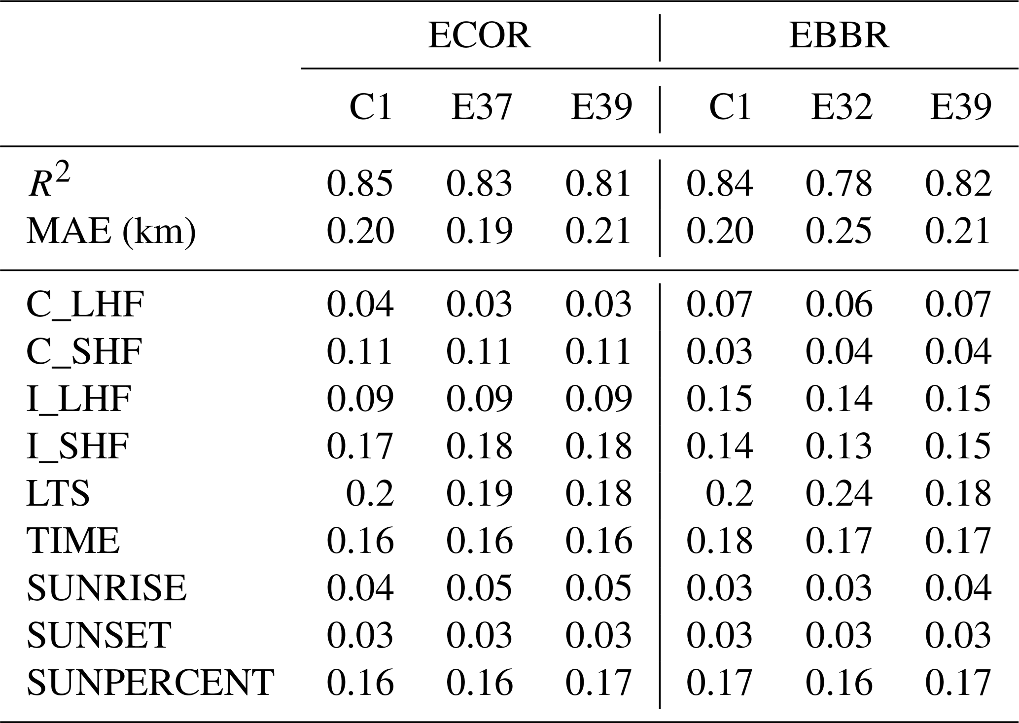
To evaluate the performance of the ECOR and EBBR models, we trained both using 70 % of the data from three sites combined and tested them on the remaining 30 % of site-specific data. The results show that ECOR outperforms EBBR overall, with an average R² of 0.83 and MAE of 0.20 across the three sites, compared to EBBR's average R² of 0.81 and MAE of 0.22. However, at site E39, EBBR achieves a slighly better R² (0.82) and MAE (0.21) than ECOR's R² (0.81) and MAE (0.21). The overall performance is only marginally better than that of training and testing solely with C1 site data: ECOR (R²: 0.85 vs. 0.85; MAE: 0.20 km vs. 0.21 km), EBBR (R²: 0.84 vs. 0.83; MAE: 0.20 km vs. 0.21 km).

In terms of input parameter importance, ECOR exhibits minimal variation, with all parameters contributing approximately 0.01, except for LTS at 0.02. For EBBR, the LTS contribution at site E32 (0.24) is 0.06 higher than at E39 (0.18). Despite E32's lower overall performance (R²: 0.78, MAE: 0.25) compared to E39 (R²: 0.82, MAE: 0.21), E32's predictions are more accurate near the CBL top (∼ 15:30 UTC−6), closely aligning with observations (mean values nearly overlap). In contrast, E39's predictions at the same time are approximately 0.1 km lower than observed. This suggests that E32's emphasis on LTS enhances prediction accuracy near the CBL top (Fig. 9), where LTS is a critical factor.

The primary influencing factors for ECOR and EBBR were similar (in Table 3), with the largest difference observed in LTS (E32: 0.24, E39: 0.18). Additionally, the allocation of SHF and LHF at E39 differed significantly between ECOR and EBBR, with notable disparities in C_LHF (0.07 vs. 0.03) and C_SHF (0.03 vs. 0.04). However, other factors, such as LTS and SUNPERCENT, showed near-identical patterns. These findings highlight discrepancies in heat flux measurements between ECOR and EBBR. Such differences typically require data assimilation in traditional PBL schemes but can be mitigated through machine learning's nonlinear combinations, yielding comparable CBLH estimates. This approach could also facilitate future heat flux data assimilation.

The lower overall R² and MAE at E32, combined with its distinct LTS contribution, indicate that local surface and meteorological conditions at E32 could differ from those at the other sites. According to Tang et al. (2019), E32 is surrounded primarily by pasture, unlike the seasonal crops and grasslands near C1 and E39, consistent with findings in Sect. 3.3. Including E32's data in training improves its performance (R²: 0.78, MAE: 0.25) compared to Sect. 3.3 (R²: 0.73, MAE: 0.27), highlighting the benefit of site-specific data in model training.

As shown in the diurnal variations across different sites (Fig. 9), noticeable discrepancies remain among them. For the model trained with the ECOR measurements, the predicted CBL top heights are lower than the observations at the C1 and E39 sites, whereas at the E37 site, the predicted values exceed the observed ones. This suggests that the entrainment process near the CBL top at E37 differs from that at C1 and E39. In contrast, the EBBR-based results show that predictions at C1 and E32 closely match the observations near the CBL top throughout the day, while at E39, the model tends to underestimate the CBL top height. Overall, the discrepancy in EBBR-based estimates is smaller than that of ECOR, particularly near the CBL top. One possible explanation is that the E39, C1, and E32 sites lie along a southeast wind trajectory, potentially leading to more consistent boundary layer characteristics across these locations (Chu et al., 2025a).

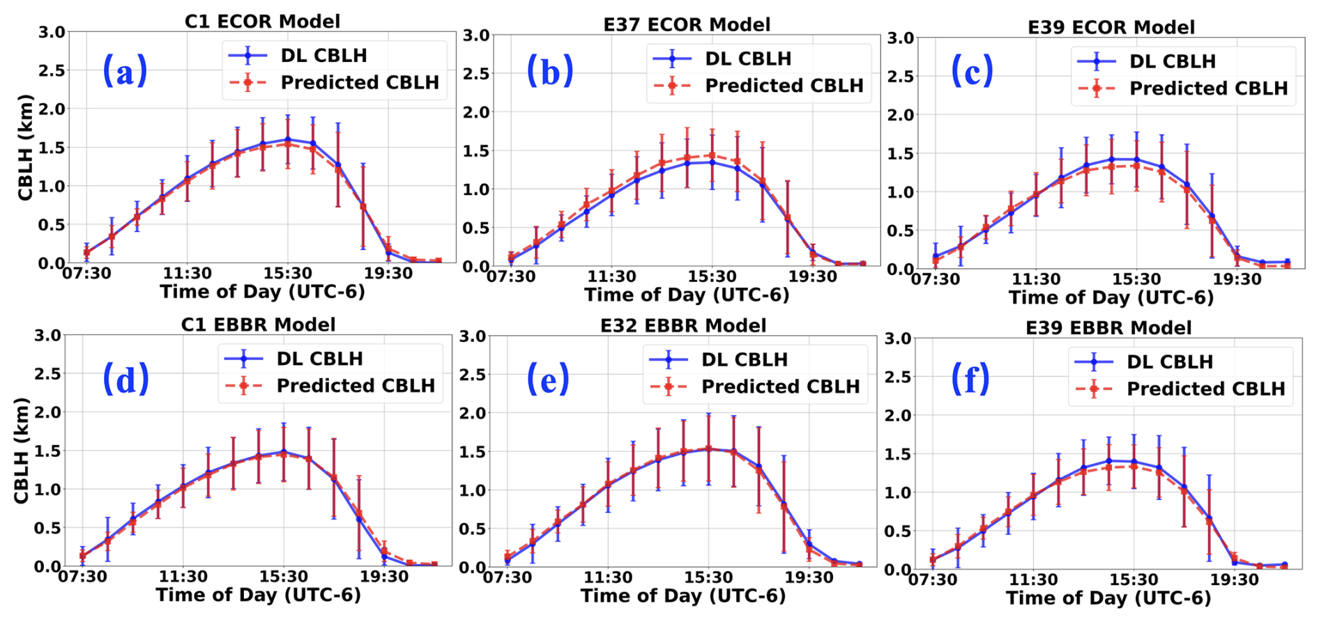
Figure 9 Diurnal variation comparison of multi-site trained models evaluated through site-specific testing. Results are grouped by heat flux measurement system: (Top) ECOR sites (a) C1 (E14), (b) E37, (c) E39; (Bottom) EBBR sites (d) C1 (E13), (e) E32, (f) E39.

4 Summary and conclusions

This study develops an Auto-ML framework for predicting CBLH, guided by thermodynamic physical constraints and the implicit diurnal cycle of CBLH. By leveraging the TPOT and the AutoKeras to automatically select optimal models, the approach bypasses manual comparisons of machine learning algorithms, enhancing efficiency and reproducibility. The resulting Auto-ML models, validated against Doppler lidar CBLH measurements, demonstrate robust performance with an overall R² of 0.84. Comparisons between ECOR and EBBR techniques for measuring surface heat and energy fluxes reveal consistent predictions, with an R² difference of approximately 0.01 and the same MAE. The models exhibit strong adaptability across multiple sites. When trained on ECOR data from the C1 site and applied to E37 and E39 sites within the ARM SGP network, the models achieve R² values of 0.79 and 0.81, respectively. Models trained on combined C1 and E39 data and tested on other sites show a gradual decline in R² and MAE with increasing distance yet maintain high predictive accuracy. These results underscore the transferability of ML models with surface flux and LTS as primary inputs based on the Auto-ML framework, highlighting its potential for integration with traditional numerical weather prediction models.

The study compared the performance of the C1 ECOR site across four seasons, revealing that summer exhibited the best performance (R²: 0.86, MAE: 0.22 km). Subsequently, the model was trained using data from multiple sites and tested individually. The overall performance surpassed that of training and testing solely with C1 site data: ECOR (R²: 0.85 vs. 0.85; MAE: 0.20 km vs. 0.21 km). ECOR sites (C1, E32, E39) generally outperformed EBBR sites (C1, E37, E39) on average, though EBBR at E39 outperformed ECOR. The primary influencing factors for ECOR and EBBR were similar, with the largest difference observed in LTS (E32: 0.24, E39: 0.18). Additionally, the allocation of SHF and LHF at E39 differed significantly between ECOR and EBBR, with notable disparities in C_LHF (0.07 vs. 0.03) and C_SHF (0.03 vs. 0.04). However, other factors, such as LTS and SUNPERCENT, showed near-identical patterns. These findings highlight discrepancies in heat flux measurements between ECOR and EBBR. Such differences typically require data assimilation in traditional PBL schemes but can be mitigated through machine learning's nonlinear combinations, yielding comparable CBLH estimates. This approach could also facilitate future heat flux data assimilation. This implicit thermodynamic physically constrained Auto-ML approach selects the best-performing machine learning model based on the dataset, improving the accuracy and generalizability of CBLH predictions across diverse sites. By providing a scalable framework for boundary layer parameterization, it offers valuable insights for refining atmospheric models and advancing the integration of machine learning in operational weather forecasting.

It should be noted that, although this study consistently refers to Auto-ML as “predicting” the CBLH, in the context of PBL schemes, it is more accurately described as “diagnosing” CBLH, given that the model uses a full day of data as both input and output. To enhance the model's applicability, it is critical to align it with the conventions of traditional PBL schemes by incorporating the CBLH output from the previous time step as an input for predicting the subsequent CBLH. Preliminary application of the model at the C1 site produces results consistent with those reported in this study (R² = 0.82; MAE = 0.20 km). The next step involves further optimization to meet additional requirements: extracting parameters from the CCPP-SCM PBL framework (Li et al., 2025) to predict the CBLH by the Auto-ML, and then feeding this output back into the PBL parameterization framework to forecast the CBLH at the subsequent time step.

The Auto-ML PBL model has broad applications due to its accuracy and efficiency. It can support air quality forecasting by better predicting pollutant dispersion within the PBL, which is crucial for urban and industrial areas (Garratt, 1992; Stensrud, 2007). Additionally, its lightweight design makes it ideal for integration into local data-driven weather forecasting systems, providing accurate CBLH inputs to support low-altitude economic activities (Ben Bouallègue et al., 2024). The Auto-ML driven scalability further enables its use in data assimilation, integrating diverse observations for improved model initialization (Arcucci et al., 2021; Arcomano et al., 2023). As observational networks like ARM expand, this model offers a versatile tool for global atmospheric research.

The lightweight Auto-ML PBL model exhibits limitations in predicting peak MLH values near the PBL top, primarily due to two interrelated factors. First, its reliance on lidar-derived training data introduces uncertainties at higher altitudes, where a reduced SNR obscures sharp inversion layers. Second, although the ML model captures energy balance constraints to some extent, it does not fully represent other critical physical processes, such as entrainment at the top of the CBL. These processes are especially important during the peak CBL development phase of the boundary layer. At this stage, shear-driven turbulence and buoyancy fluxes play a dominant role in promoting vertical mixing and facilitating the entrainment of free-atmosphere air into the CBL. Without explicitly incorporating these mechanisms, the model may underrepresent key drivers of boundary layer growth, particularly under conditions of strong surface heating or elevated wind shear. This limitation highlights the need for physically informed hybrid models that can integrate data-driven approaches with boundary-layer process understanding. Unlike traditional schemes that parameterize these through TKE budgets or non-local mixing, the Auto-ML model lacks such dynamic constraints, reducing its sensitivity to abrupt inversion layer changes or synoptic-scale forcings (e.g., advective momentum fluxes) (Stevens, 2002; Cuxart et al., 2006; Fernando, 2010; Shin et al., 2021;). The IQR for predicted CBLH is consistently narrower than those for DL-derived CBLH across all seasons, reflecting lower variability in predicted CBLH (based on thermodynamic parameters) compared to DL-derived CBLH, which is influenced by additional factors such as wind and low-level jets. Despite these limitations, a follow-up work is underway to develop an AI/ML-based emulator for parameterizing PBL, which will be applied to real-case simulations to assess its performance against conventional PBL schemes. To enhance the model, future work will integrate additional boundary-layer parameters, such as wind speed, direction, shear, veer, surface upwelling and downwelling longwave and shortwave radiation, as well as ceilometer-derived cloud fraction and base height, utilizing data from ARM sites. High-resolution observations (e.g., uncrewed aircraft systems or airborne lidar) will also be explored to directly sample the entrainment zone, enhancing physical understanding of entrainment. Additionally, integrating parameters like turbulent dissipation rate (Chu et al., 2025b) could refine predictions of PBL variables, enabling a more comprehensive parameterization scheme.