Impacts of mesoscale atmospheric subsidence on cloud glaciation and decoupling in Arctic marine cold air outbreaks

The impact of mesoscale vertical atmospheric motion on the thermodynamic, microphysical, and convective transformations of air masses during marine cold air outbreaks (MCAOs) is largely unknown, partly due to scarcity of suitable observations in Arctic regions. To help close this gap, this study investigates the effects of mesoscale subsidence on the evolution of atmospheric boundary-layer (ABL) properties, cloud phase, and precipitation characteristics for a case study of a shallow MCAO observed in the Fram Strait during the HALO–(𝒜𝒞)³ campaign in March 2022. Quasi-Lagrangian Large-Eddy Simulations (LES) are conducted with observational initialisation and larger-scale forcing, based on airborne in-situ and remote-sensing measurements. The LES control simulation accurately reproduces the measured thermodynamic ABL structure and the temporal evolution of the observed air mass moving over the Arctic sea ice onto the open ocean. Specifically, the measured ABL height, integrated water vapour, and cloud water paths are well represented by the LES control run. Sensitivity experiments using the LES assuming prescribed subsidence reveal that weaker subsidence substantially deepens the ABL and causes an earlier onset of cloud glaciation. Decoupling of the cloud layer occurs sooner under weaker mesoscale subsidence, triggering convective graupel formation. This link between glaciation and decoupling explains the typical evolution of the cloud liquid water path observed in many MCAOs.

1 Introduction

During marine cold air outbreaks (MCAOs), cold and dry polar air masses are advected over cold sea ice surfaces towards the warmer open ocean, where they heat up and pick up humidity from below. MCAOs are an essential phenomenon in the Arctic climate system that frequently occurs over extended marine regions at northern high latitudes (Fletcher et al., 2016). Additionally, as these air masses cross the sea ice edge and move over open ocean, the strong near-surface air temperature contrast between the warmer open ocean surface and the overlaying colder air generates intense turbulent and convective mixing, producing large sensible vertical heat fluxes (Shapiro et al., 1987; Renfrew and Moore, 1999; Papritz et al., 2015; Kirbus et al., 2023). This vertical turbulent exchange rapidly transforms the air mass and deepens the Atmospheric Boundary Layer (ABL). As a result, spatially organised cloud structures evolve in the ABL that initially appear as cloud streets (Atkinson and Wu Zhang, 1996; Lenschow and Agee, 1976; Etling and Brown, 1993; Kirbus et al., 2024; Klingebiel et al., 2025). As the air mass continues to respond to the warm open ocean surface, low-level warming and moistening, together with persistent vertical surface energy flows, precipitation, and cloud microphysical processes such as riming and secondary ice production promotes a transition from cloud streets to deeper, broken cloud fields (Tornow et al., 2021; Murray-Watson et al., 2023; Schirmacher et al., 2024). These evolving cloud and ABL characteristics modulate cloud-radiative interactions, determine precipitation formation, and increase surface winds (Kolstad, 2017; Terpstra et al., 2021; Mateling et al., 2023). Through this ocean–atmosphere coupling, MCAOs influence atmospheric and oceanic circulations (Rasmussen et al., 1992; Isachsen et al., 2013; Papritz and Spengler, 2017; Marcheggiani and Spengler, 2025), which are linked to feedback mechanisms of Arctic amplification (Wendisch et al., 2023). The air mass transports during MCAOs and the corresponding transformation processes also contribute to heat and moisture exchange between the Arctic and mid-latitudes (Pithan et al., 2018).

Despite extensive prior studies, key aspects of MCAO evolution remain poorly understood, particularly the onset of ABL decoupling in the sub-cloud layer, which accelerates stratocumulus breakup and promotes transitions between cloud regimes (Bretherton and Wyant, 1997; McCoy et al., 2017; Lloyd et al., 2018; Zhou et al., 2015). Furthermore, precipitation formation and cloud microphysical developments that are influenced by riming and secondary ice production, reducing vertical mixing and altering ABL energy budgets, are not well represented in models (Abel et al., 2017; Karalis et al., 2022; Wu et al., 2025). Persistent observational gaps, particularly in remote upstream regions of MCAO pathways, continue to limit our understanding of these processes and their role in organising MCAO transitions. Consequently, major questions remain regarding how dynamical and microphysical processes support the transition to open-cell convection and how these should be represented in numerical models (Tomassini et al., 2017; de Roode et al., 2019).

The role of mesoscale vertical motion in MCAO evolution, and mixed-phase clouds in particular, is complex and not yet fully understood. Previous studies have shown that subsidence in surface-coupled convective layers can counteract mixed-layer growth by reducing the effective contributions of cloud-top entrainment. Increased liquid water paths inside the mixed-layer can enhance cloud-top radiative cooling and, together with precipitation-related diabatic processes, promote convective overturning and precipitation production. In turn, enhanced cloud-top radiative cooling and convective overturning under stronger subsidence can increase precipitation production in both rain and snow. Under surface-warming conditions, stronger subsidence can also suppress cloud-top ascent and help maintain a stable stratiform cloud layer (Young et al., 2018).

In contrast, Neggers et al. (2019) found that strong subsidence can cause mixed-phase cloud layers over the central Arctic sea ice to collapse, shifting thermal-infrared radiative cooling to the surface and hindering cloud reformation. These findings highlight that mesoscale subsidence can strongly modulate mixed-phase cloud layers, although it remains unknown how this modulation depends on the ABL structure. The involved interactions span a wide range of spatial scales, from mesoscale to synoptic subsidence. It covers processes such as turbulent entrainment, microphysical interactions, and aerosol particle evolution (Tornow et al., 2021, 2023). A prime cause for our lack of insight into the impact of mesoscale subsidence on mixed-phase clouds is the distinct observational data gap on this variable at high latitudes. Measuring large-scale vertical motion or horizontal divergence remains difficult, as small errors in horizontal wind gradients lead to large uncertainties when using mass conservation. A more robust method applies regression to dropsonde data released in mesoscale patterns by fast aircraft, pioneered during two aircraft campaigns in the subtropical trades (Bony and Stevens, 2019; Stevens et al., 2021; George et al., 2021). The application of this method to the coherent flow of an Arctic MCAO, as realized in this paper, helps to narrow this data gap and to enhance our understanding of the impacts of subsidence on the development of mixed-phase clouds in growing atmospheric boundary layers.

The Fram Strait in the North Atlantic Ocean is a hotspot for MCAOs. It is relatively easy to access, making it a frequent target area for atmospheric observational and modelling studies. Although many recent Fram Strait studies are model-based, several field campaigns have filled key data gaps of MCAO processes. For example, the Cold air Outbreaks in the Marine Boundary Layer Experiment (COMBLE) in 2019 and 2020 observed several MCAOs with two permanent observational sites that provided continuous measurements of downstream conditions at Bear Island and Andenes (Geerts et al., 2022), and the Springtime Atmospheric Boundary Layer Experiment (STABLE) campaign in March 2013 and the Cold Air Outbreak Experiment in the Sub-Arctic Region (CAESAR), who provided airborne observations with research aircraft in the Fram Strait (Michaelis et al., 2022; Zuidema et al., 2026). The HALO–(𝒜𝒞)³ campaign in 2022 sampled numerous MCAOs with multiple co-located aircraft, probing upstream and downstream regions (Walbröl et al., 2024; Wendisch et al., 2024, 2025; Ehrlich et al., 2025). During HALO–(𝒜𝒞)³, the mesoscale dropsonde pattern technique was applied to sample mesoscale atmospheric subsidence at multiple points along a MCAO trajectory for two consecutive days, producing the first robust high-latitude subsidence dataset of its kind (Paulus et al., 2024). This unique dataset creates new opportunities for investigating the role of subsidence in MCAO evolution.

The main objective of this study is to use quasi-Lagrangian Large-Eddy Simulations (LES), driven by HALO–(𝒜𝒞)³ observational data, to gain insight into the impacts of mesoscale subsidence on MCAOs. For a particular case study, the LES follows an observed MCAO along its 2 d southbound trajectory, initialised with in-situ dropsonde profiles from the High Altitude and Long Range Aircraft (HALO) in the far north. The simulated air mass evolves freely, with large-scale forcings, including vertical motion, geostrophic wind, and advection tendencies, derived from circular dropsonde pattern observations and prescribed along the trajectory (Paulus et al., 2024). The simulated ABL and cloud properties are compared against independent downstream aircraft observations.

Given this observationally constrained model setup, we ask how well the Lagrangian LES reproduces the independently observed cloud development. After evaluating the model performance, we conduct perturbation experiments on the mesoscale subsidence to assess the sensitivity of the MCAO, focusing on the evolution of the ABL structure, cloud mass, thermodynamic phase, and surface precipitation. This study aims to discuss how microphysical and dynamical properties and processes interact in their response to perturbed larger-scale subsidence forcing within the simulated MCAO system.

2 Observations

2.1 The HALO–(𝒜𝒞)³ campaign

The HALO–(𝒜𝒞)³ field campaign took place in the Norwegian/Greenland Seas and the Fram Strait from March to April 2022. The main objective of this airborne campaign was to understand the transformation of air masses between the Arctic and the mid-latitudes and to investigate the influence of these interactions on ABL processes and cloud formation. To this end, a quasi-Lagrangian sampling strategy was applied during the campaign, in which the transformation of individual air parcels of an air mass was tracked along their trajectories using three research aircraft flying at different altitudes (HALO, Polar 5, and Polar 6) (Wendisch et al., 2024). An overview of the synoptic situation during the HALO–(𝒜𝒞)³ campaign is provided by Walbröl et al. (2024).

This study focuses on a case study analysing two HALO Research Flights 10 and 11 (RF10 and RF11) conducted on 29 and 30 March 2022 (Fig. 1). On these 2 d, a weak MCAO with an MCAO index of four was investigated (Papritz and Spengler, 2017; Walbröl et al., 2024) (Appendix B). Both days were characterised by a persistent northerly wind of about 3 to 10 m s⁻¹ measured at 10 m altitude by dropsonde observations. These characteristics indicate a weak MCAO event compared with climatological values from the Fram Strait (Slättberg et al., 2025). The slowly moving air mass was probed by HALO during these 2 d. The observed MCAO case embedded within a prolonged period of extensive MCAO activity from 21 March to 12 April 2022, between two intervals of particularly strong conditions on 21–26 March and 1–2 April 2022 (Walbröl et al., 2024).

The synoptic situation in the Fram Strait was characterised by a high-pressure system centred at the east coast of Greenland and a low-pressure area in the Barents Sea (Fig. A1). The cloud field was dominated by shallow convective mixed-phase clouds, with obvious street features near the sea ice edge. These cloud streets broke up further downstream in the area of C03 (Fig. 1). A notable cloud-free area was located on the west coast of Svalbard (Fig. 2), which can be attributed to the Foehn effect during easterly flow over Svalbard, similarly observed during other field campaigns (e.g., Shestakova et al., 2022).

The HALO flight plans on these 2 d aimed at tracking the location of an air mass sampled on the first day at a location in the high north above sea ice using trajectory estimates based on forecast data. At four locations along the trajectory, the air mass was sampled using a circular mesoscale dropsonde pattern, with a diameter of 150 km. This technique is inspired by Lenschow et al. (2007) and has been applied in the North Atlantic and subtropical region by Stevens et al. (2019, 2021) to measure mesoscale divergence and subsidence profiles. The centre of the initial circle (IC) (Fig. 1) on the first day at 14:00 UTC was located at (84.4° N, 13.6° E) and featured only five dropsondes, a number limited by airspace restrictions. On the second day, three further circular patterns were flown along the predicted southern trajectory of the air mass. The circles sampled during the two subsequent days featured eight evenly distributed dropsondes, with two additional dropsondes launched in their inner areas. Only one of the day-two circles, (C02) at (78.6° N, 4.0° E, at 11:30 UTC), was located at the exact predicted location of the air mass as sampled on the previous day at the IC location. As shown in Fig. 1, this circle was situated over open ocean. Two further circles were flown on day two, one (C01) further upstream over sea ice (80.8° N, 10.7° E, at 10:30 UTC), and another (C03) was flown at a downstream location at a similar distance (76.3° N, 3.3° E, at 12:30 UTC). The Polar 5 (P5) aircraft took additional measurements in the C02 area, shortly after the departure of the HALO aircraft from this area (at 12:00 UTC), using a rectangular flight pattern with three cross-flow legs. Additional measurements were conducted by a controlled meteorological balloon (CMET) launched from Ny-Ålesund, as part of the ISLAS2022 field experiment (Sodemann, 2023), which took place at the same time as the HALO–(𝒜𝒞)³ campaign.

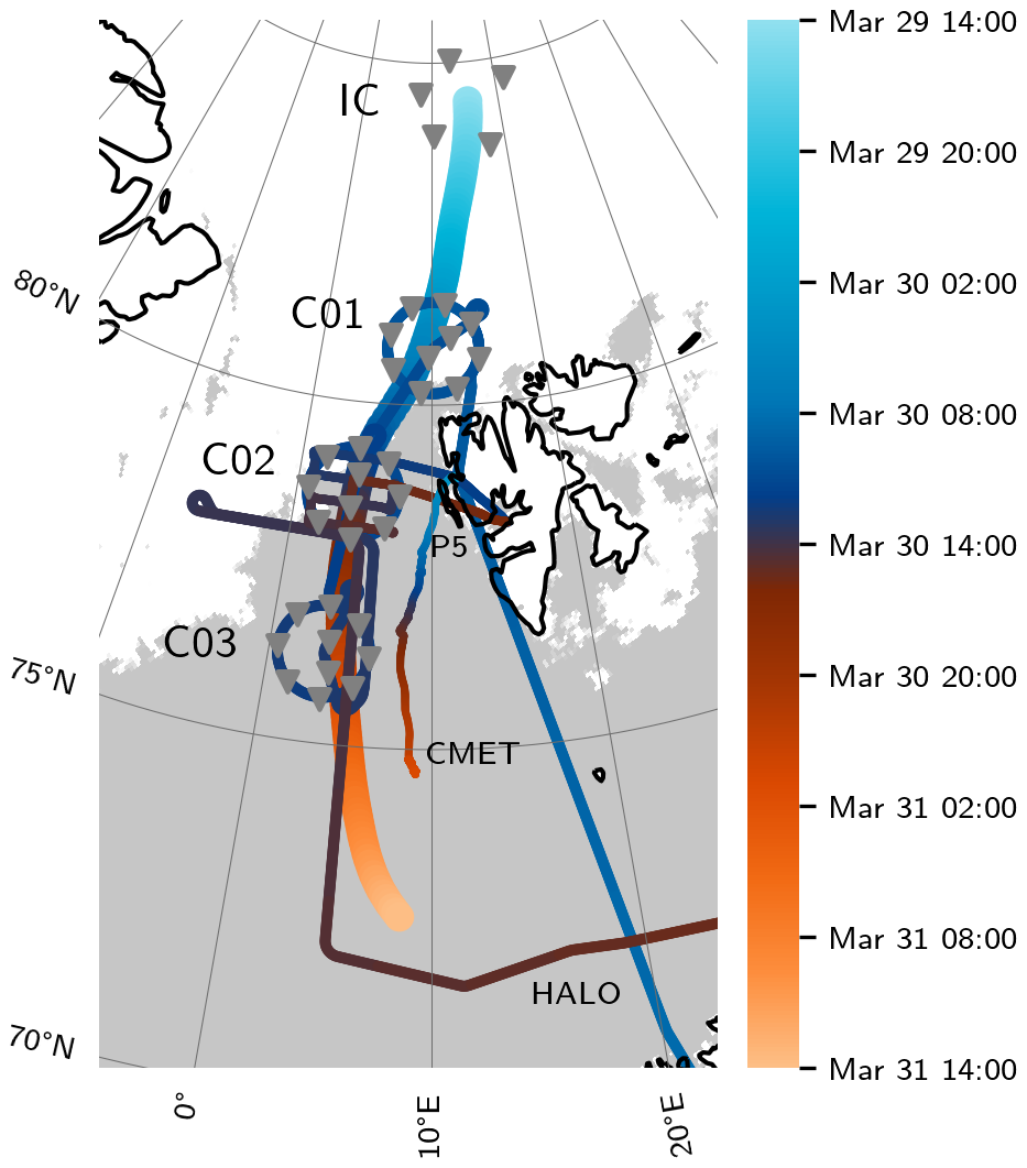
Figure 1 Map of the simulation trajectory for the Lagrangian LES (bold line) initiated in the centre of the circular flight leg on 29 March 2022 of the HALO–(𝒜𝒞)³ campaign, together with the flight paths of the HALO and P5 aircraft on 30 March 2022 and the trajectory of the CMET. Locations where dropsondes were released in IC on 29 March 2022 and in C01, C02 and C03 of 30 March 2022 from HALO are indicated by ▾. The sea ice concentration retrieved from satellite observations (Spreen et al., 2008) is indicated in grey and white, and the colour bar denotes the time (UTC) along the trajectory and flight paths.

2.2 Data

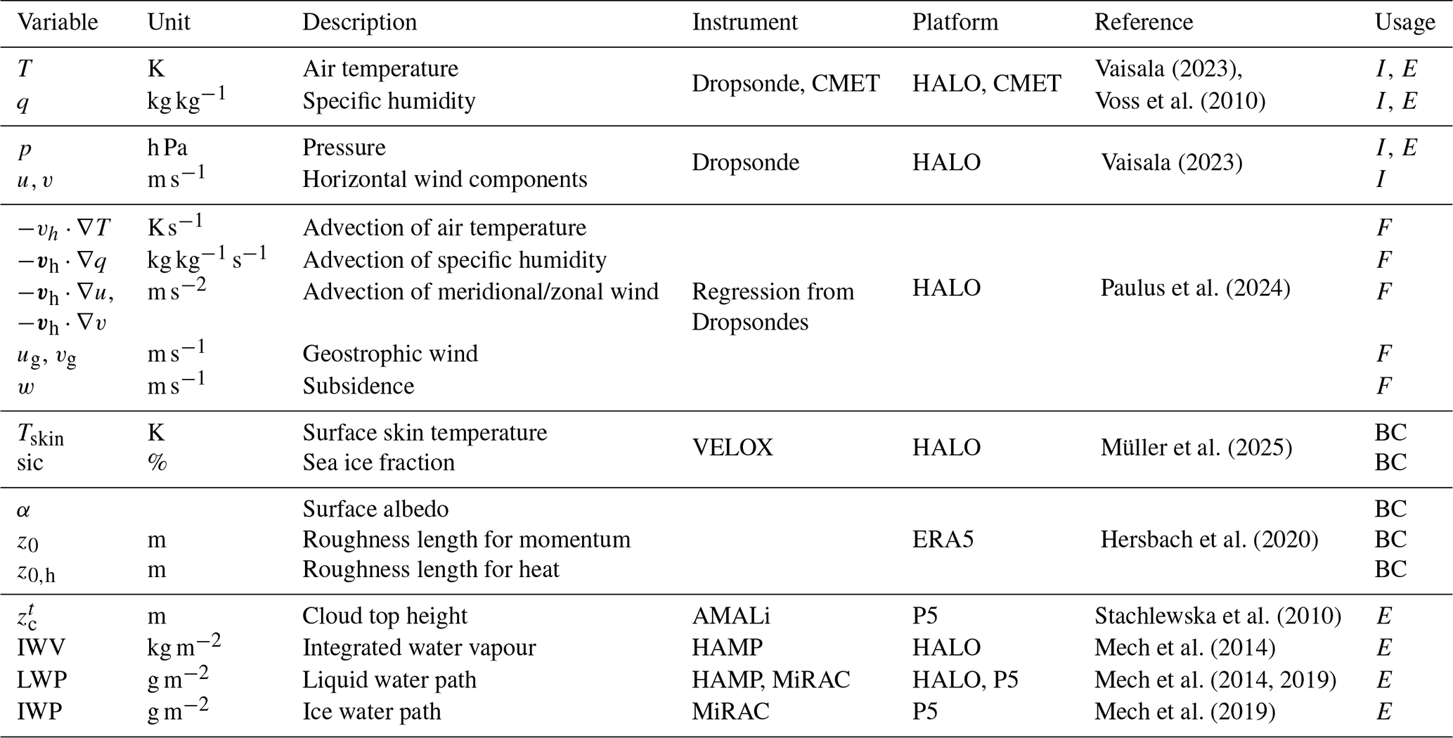
A combination of in-situ and remote sensing observations from the HALO–(𝒜𝒞)³ campaign were used to constrain the LES experiments and evaluate the model performance. A comprehensive overview of the measurements collected during HALO–(𝒜𝒞)³ is described by Ehrlich et al. (2025), and a summary of the datasets used is presented in Table 1, including the variable names, associated instruments, and references to more detailed technical and scientific descriptions.

The deployed Vaisala RD-41 dropsondes provide vertical profile measurements of the thermodynamic state, including air temperature at a resolution of 0.01 K, relative humidity at a resolution of 0.1 % and air pressure at a resolution of 0.01 h Pa at frequencies between 2 and 4 Hz and descend at speeds between 10 and 20 m s⁻¹ (Vaisala, 2023). The measured profiles are interpolated to a uniform vertical grid of 5 m spacing. The horizontal wind speed profiles were determined from GPS data with an estimated accuracy of 0.1 m s⁻¹ (Hock and Franklin, 1999; Wang et al., 2015). These observations were used to derive vertical profiles of subsidence (Fig. 3), geostrophic wind, and advective tendencies of temperature, humidity, and wind through a regression algorithm applied to the dropsondes deployed in each circle. A comprehensive description of the calculation technique is provided by Paulus et al. (2024).

To constrain the surface skin temperature T_skin, airborne measurements of the thermal-infrared imager on board HALO VELOX (Video airbornE Longwave Observations within siX channels; Schäfer et al., 2022) were used, which records 2-D fields (640×512 px) of the thermal infrared brightness temperature. At typical HALO flight altitudes, this corresponds to a horizontal resolution of 10 m with a temporal resolution of 1 Hz for a field-of-view of 6.4×5.1 km. From these brightness temperature images, the skin temperature T_skin and sea-ice concentration were derived along the circular flight legs of HALO with estimated measurement uncertainties of 1.2 K and 5 %, respectively (Müller et al., 2025). For partly cloudy open-ocean segments in C02 and C03, we apply a cloud mask and classify pixels whose retrieved values of T_skin exceed −1.8 °C above the surrounding (cloudy) background as open ocean. The final surface skin temperature is the horizontal mean of each masked 2D-field at a 1 Hz time resolution.

The datasets collected during the HALO–(𝒜𝒞)³ campaign provide all atmospheric state variables required to run Lagrangian LES experiments following the air mass as it moves south. A small number of surface parameters, such as the surface albedo, the aerodynamic roughness length for momentum, and the thermal roughness length for heat, could not be measured, but are needed to prescribe the (latitude-dependent) surface boundary condition in the LES experiments. Therefore, these data were retrieved from the European Centre for Medium-Range Weather Forecasts (ECMWF) reanalysis product version 5 (ERA5; Hersbach et al., 2020). By combining the dropsonde and VELOX observations with the surface values from ERA5, a complete set of forcing fields for the Lagrangian LES has been compiled.

For model validation, independent datasets obtained from the HALO–(𝒜𝒞)³ campaign are used. The Airborne Mobile Aerosol Lidar (AMALi) on the P5 aircraft provides measurements of cloud top height, which are compared to the simulated cloud top heights (Stachlewska et al., 2010). The liquid water and ice water paths are derived from the Microwave Radar/Radiometer for Arctic Clouds (MiRAC) on board P5 (Mech et al., 2019). The ice water path is derived from the 94 GHz-radar reflectivity using the Ze–IWC relationship of Hogan et al. (2006). We additionally include integrated water vapour (IWV) and liquid water path (LWP) data retrieved from the HALO Microwave Package (HAMP) over open ocean (not available over sea ice) (Mech et al., 2014). These data allow a direct comparison with the quantities computed by the LES.

Further thermodynamic observations were performed using Lagrangian CMET soundings (Voss et al., 2010). The balloon was equipped with an air temperature sensor that operates over a range of −40 to 105 °C with an interchangeability of ±0.5 °C and measured relative humidity with respect to water with an accuracy of 1.5 %. Due to the cold, dry conditions, and the absence of active ventilation of the sensor package on the CMET, actual measurement errors would be substantially larger than the sensor interchangability, in particular during daytime when the balloon was drifting horizontally, creating an overall warm and dry bias. This particular CMET-04 was launched in Ny-Ålesund on 30 March 2022 at 14:00 UTC following a trajectory parallel to the simulated trajectory (Fig. 1), complementing the dropsonde observations and providing additional in-situ validation data within the lower ABL.

Vaisala (2023)Voss et al. (2010)Vaisala (2023)Paulus et al. (2024)Müller et al. (2025)Hersbach et al. (2020)Stachlewska et al. (2010)Mech et al. (2014)Mech et al. (2014, 2019)Mech et al. (2019)

Table 1 Variables used in the LES for initialisation (I), evaluation (E), boundary condition (BC) and larger scale forcing (F).

3 Model configuration

3.1 The Dutch Atmospheric Large-Eddy Simulation Model (DALES)

The simulations were performed using the Dutch Atmospheric Large-Eddy Simulation (DALES) (Heus et al., 2010), which is an open-source model available at https://github.com/dalesteam/dales (last access: 2 October 2026). DALES has been tested and applied extensively in previous studies of ABL turbulence and clouds in various regions of the Earth (van der Dussen et al., 2013; Corbetta et al., 2015; Roode et al., 2016; Laar et al., 2019; Reilly et al., 2020), including the Arctic (Neggers et al., 2019; de Roode et al., 2019; Egerer et al., 2021; Chylik et al., 2023; Schnierstein et al., 2024).

To represent Arctic mixed-phase clouds, the DALES code was equipped with the double-moment microphysics scheme of Seifert and Beheng (2006), which is predictive of both the mass and number concentrations of five hydrometeor classes (cloud water, cloud ice, rain, snow, and graupel) (Neggers et al., 2019; Chylik et al., 2023). The number concentration of cloud condensation nuclei (CCN) is prognostic, initialised with a constant vertical profile of 100 cm⁻³ within the range observed during the HALO–(𝒜𝒞)³ campaign in the Fram Strait (Wendisch et al., 2024) and in the high Arctic during MOSAiC (Ansmann et al., 2023). The available INP number concentration is prescribed with an upper limit of $\mathrm{1}\times {\mathrm{10}}^{-\mathrm{3}}$ cm⁻³, following the setup of Chylik et al. (2023) and Hartmann et al. (2019), while the activated fraction depends on temperature and ice supersaturation through the Reisner et al. (1998) parametrisation. Heterogeneous freezing processes are limited to temperatures below −15 °C, and the maximum number of ice particles resulting from deposition nucleation is restricted to 200 L⁻¹, while homogeneous freezing and secondary ice formation via the Hallett-Mossop process remain unchanged as represented in the Seifert and Beheng (2006) model. This microphysical model setup was thoroughly tested by Schnierstein et al. (2024) against a year of in-situ measurements of Arctic clouds in the central Arctic during the MOSAiC expedition.

Further model settings follow the setup described by Schnierstein et al. (2024). They include a radiative transfer scheme interactive with liquid and ice hydrometeors applying a four-stream radiative transfer solver in combination with Monte Carlo spectral integration (Pincus and Stevens, 2009). The optical properties of ice particles are based on the physical properties of the ice crystals derived from the microphysics scheme (McFarquhar and Heymsfield, 1998; Fu and Liou, 1993; Baran, 2005; Schnierstein et al., 2024). Resolved advection is calculated using a fifth-order central difference numerical scheme for momentum and a κ-limiter scheme for the other prognostic scalar variables. Subgrid-scale transport uses a prognostic turbulent kinetic energy (SFS-TKE) scheme (Deardorff, 1980; Hundsdorfer et al., 1995). A sponge layer is applied in the upper 25 % of the range to dampen disruptive gravity waves. The surface fluxes of heat, moisture, and momentum are calculated based on Monin-Obukhov theory using Arctic stability functions derived by Grachev et al. (2007). Horizontally periodic boundary conditions are applied, while large-scale forcings are prescribed as time-dependent tendency profiles to account for advection, subsidence, and horizontal pressure gradients (geostrophic wind vector v_g).

3.2 Trajectory calculation

To set up a Lagrangian LES experiment, the trajectories (pathways) of the air parcels forming the air mass need to be estimated. Trajectories for the low-level air parcels were calculated during flight planning using the Lagrangian Analysis Tool (LAGRANTO) (Sprenger and Wernli, 2015) and based on IFS forecast winds. For this study, this was repeated using 3-D wind fields of the ERA5 reanalysis. Air parcels were identified, and their trajectories were calculated starting every 3 km lat/lon within the IC on 29 March 2022 and passed through the circle locations on 30 March 2022 (Kirbus et al., 2024). The best match of the trajectories was found at 870 hPa in the initiation region. For the simulations, a mean trajectory was calculated by averaging all trajectories initiated within the first circle at 870 hPa. Each trajectory is included for every circle region it intersects, but is excluded from further analysis once it exits a circle region without entering the subsequent one. This procedure is illustrated in Fig. C1.

3.3 Observational forcing and boundary conditions

The lower boundary conditions are prescribed as time-varying fields along the Lagrangian simulation trajectory with hourly resolution. Surface skin temperature T_skin and sea-ice concentration “sic” are derived from VELOX observations (Sect. 2.2), longitudinally averaged along the circular flight legs, and interpolated along the simulation trajectory. As the simulated air mass moves from sea ice through the marginal ice zone to the open ocean, this interpolation provides a temporally evolving surface boundary condition. The lower-boundary specific humidity is calculated following Schnierstein et al. (2024) from the saturation specific humidity at the prescribed surface skin temperature and weighted by the local sea-ice fraction.

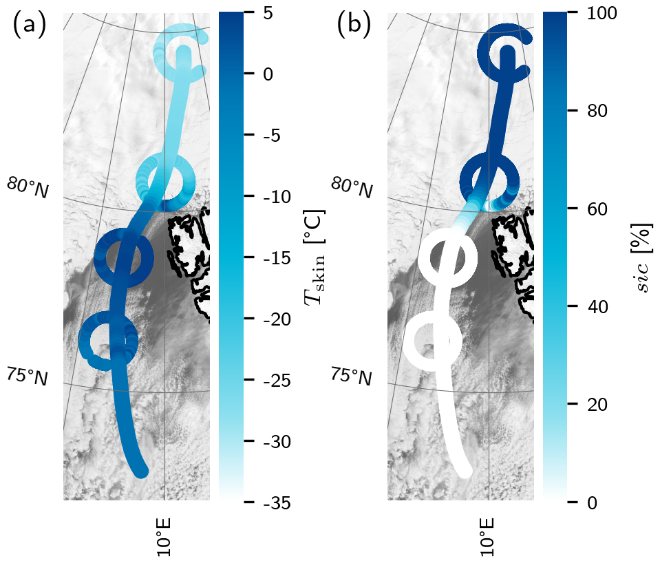
Figure 2 VELOX observations of surface skin temperature (T_skin) and sea ice concentration “sic” on the circular flight legs of the HALO flights on 29 March and 30 March 2022 during HALO–(𝒜𝒞)³ (circles), together with interpolated T_skin and “sic” along the LES trajectory used as surface boundary conditions (bold line).

The prescribed large-scale forcing profiles are time-dependent and they are obtained by interpolation along the trajectory between the sonde data at the four circle locations. A regression algorithm is used to estimate horizontal gradients within each circle area, following the method of Bony and Stevens (2019). The horizontal wind divergence and the associated subsidence ω are calculated as described by Paulus et al. (2024). At high latitudes, Cartesian latitude–longitude coordinates distort horizontal distances. To address this issue, Paulus et al. (2024) introduced a regression method in spherical coordinates $\left[r,\mathit{\phi },\mathit{\theta }\right]$. Assuming linear fluctuations of any variable $\mathit{\xi }\in \left[u,v,q,T,p\right]$ within the dropsonde area, ξ at the centre of the pattern can then be approximated at every vertical level by a first-order Taylor expansion:

$$\begin{array}{}\text{(1)}& \mathit{\xi }={\mathit{\xi }}_{\mathrm{0}}+{\displaystyle \frac{\partial \mathit{\xi }}{\partial \mathit{\theta }}}\mathrm{\Delta }\mathit{\theta }+{\displaystyle \frac{\partial \mathit{\xi }}{\partial \mathit{\phi }}}\mathrm{\Delta }\mathit{\phi }.\end{array}$$

Here, ξ₀ denotes the mean of all dropsonde measurements, and θ and φ are the polar and azimuth angles, respectively. This approach is applied in this study to estimate divergence:

$$\begin{array}{}\text{(2)}& D=\mathbf{\nabla }\cdot v_h={\displaystyle \frac{\mathrm{1}}{r\cdot \sin \mathit{\theta }}}\left[{\displaystyle \frac{\partial u}{\partial \mathit{\phi }}}+{\displaystyle \frac{\partial \sin \mathit{\theta }v}{\partial \mathit{\theta }}}\right].\end{array}$$

This allows for the estimation of the associated subsidence at height z by vertical integration from the surface:

$$\begin{array}{}\text{(3)}& \mathit{\omega }=-g\cdot \mathit{\varrho }\underset{\mathrm{0}}{\overset{z}{\int }}D\mathrm{d}z.\end{array}$$

Figure 3 shows the resulting subsidence profiles in the four circles, provided in pressure and height units for reference, with key characteristics summarised in Table C1. In IC and C02, subsidence dominates the lowest 3 km, with mean downward motions of −0.74 and −0.60 cm s⁻¹, respectively, while C03 exhibits weaker subsidence throughout the profile. In contrast, C01 shows a mean upward motion over the 8 km profile. Uncertainties associated with the regression-based divergence estimate were calculated following Paulus et al. (2024) and reach up to 0.025 cm s⁻¹ (0.002 Pa s⁻¹) below 3 km across all circles, which cannot be resolved in the figure and are therefore not shown. These estimates reflect uncertainties propagated from the regression analysis and do not represent a complete uncertainty budget, as they exclude potential representativeness errors associated with temporal evolution during the sequential dropsonde releases and deformation of the sampling pattern due to horizontal sonde drift. The method assumes approximate stationarity over the sampling period; sensitivity tests by Paulus et al. (2024) indicate that accounting for pattern deformation changes the derived divergence and pressure velocity by less than 1 % and 10 %, respectively. The subsidence magnitudes are consistent with reanalysis-based estimates of Arctic MCAOs (Paulus et al., 2024; Tornow et al., 2023), but are approximately an order of magnitude lower than those reported for the tropical Atlantic, possibly due to the specific weather conditions of the sampled case (Bony and Stevens, 2019; George et al., 2021).

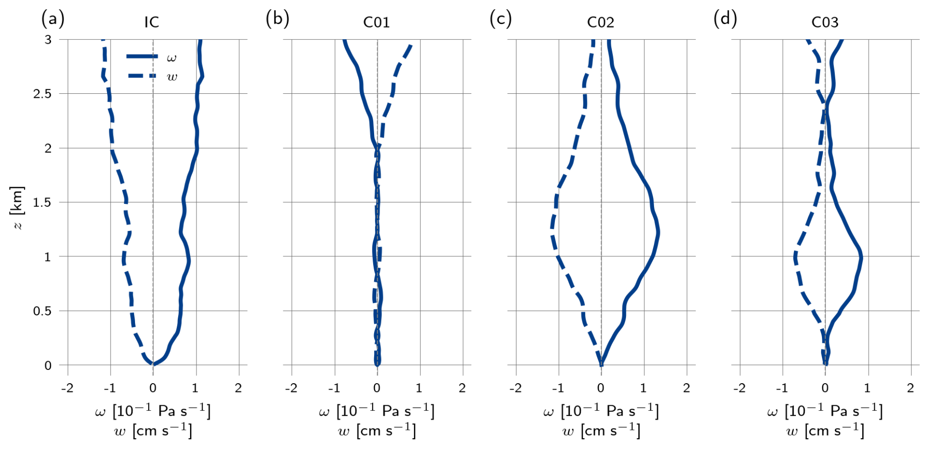
Figure 3 Subsidence profiles obtained through regression from a dropsonde pattern in pressure (ω, solid line) and height (w, dashed line) coordinate for all dropsonde patterns on 29 March and 30 March 2022 of the HALO–(𝒜𝒞)³ campaign. Associated uncertainty estimates cannot be resolved in the figure and are discussed in the main text.

The same regression approach using spherical coordinates can be applied to calculate the horizontal advective tendencies in the circular areas,

$$\begin{array}{}\text{(4)}& -{\mathit{v}}_{\mathrm{h}}\cdot \mathbf{\nabla }\mathit{\xi }=-\left[u{\displaystyle \frac{\mathrm{1}}{r}}{\displaystyle \frac{\partial \mathit{\xi }}{\partial \mathit{\theta }}}+{\displaystyle \frac{\mathrm{1}}{r\cdot \sin \mathit{\theta }}}{\displaystyle \frac{\partial \mathit{\xi }}{\partial \mathit{\phi }}}\right],\end{array}$$

and similarly, the horizontal pressure gradient force, here expressed as the geostrophic wind vector v_g,

$$\begin{array}{}\text{(5)}& {\mathit{v}}_{\mathrm{g}}={\displaystyle \frac{\mathrm{1}}{\mathit{\varrho }\cdot f}}\cdot \left(\begin{array}{c}\frac{\partial p}{\partial \mathit{\phi }}\\ \frac{\mathrm{1}}{\cos \mathit{\phi }}\frac{\partial p}{\partial \mathit{\theta }}\end{array}\right).\end{array}$$

These profiles, which extend up to HALO's flight altitude at about 8 km, are linearly interpolated between the four circles and kept constant south of the last circle along the simulation trajectory (Fig. 4). What stands out in the interpolated mesoscale vertical pressure velocity field ω(t,z) is the distinct maximum at C02 below 4 km, which indicates a relatively strong signal in the prescribed subsidence that will play a crucial role in this study. Concerning the advective tendencies, the temperature advection $-{\mathit{v}}_{\mathrm{h}}\cdot \mathbf{\nabla }T$ is dominated by cooling at low altitudes, below 1 km. The specific humidity exhibits low-level drying before the sea ice edge, transitioning to moistening south of C02. The horizontal wind components show low signals, except for a slight positive tendency of the meridional wind in the deepening ABL south of C01. These likely reflect Ekman-layer effects of Reynolds stresses, inducing a deviation of the wind from the geostrophic wind direction. The geostrophic wind ($\left|{\mathit{v}}_{\mathrm{g}}\right|$) expresses an eastward zonal pressure gradient force throughout the lower levels, consistent with the general synoptic situation during the 2 d. It should be noted that at a trajectory height of 870 h Pa corresponding to heights between 1.34 and 1.38 km, advective tendencies are, by definition, zero, as the air mass speed is subtracted from the wind in the Lagrangian forcing method.

Above 8 km altitude, which is well above the simulated ABL height (max 2 km), the sonde data are extended by ERA5 fields. The main objective of this procedure is to allow radiative flux density (irradiance) calculations above the model domain in which turbulence is resolved, which has a ceiling far below HALO's flight altitude (described in Sect. 3.4). As a result, it is concluded that the use of ERA5 fields above this height has no discernible impact on the model results.

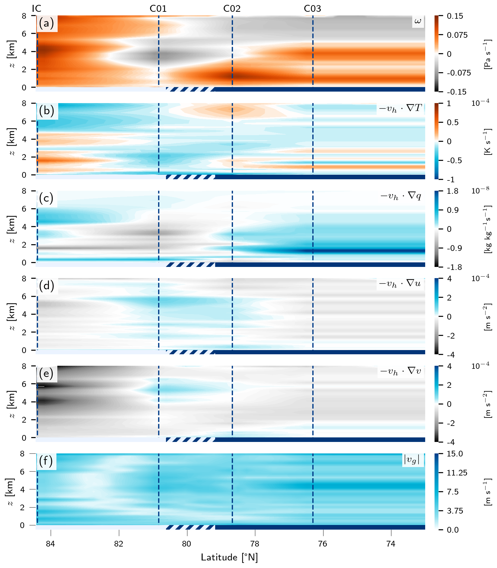
Figure 4 Simulation forcing of subsidence ω (Ctrl) (a), horizontal temperature advection $-{\mathit{v}}_{\mathrm{h}}\cdot \mathrm{\nabla }T$ (b), horizontal humidity advection $-{\mathit{v}}_{\mathrm{h}}\cdot \mathrm{\nabla }q$ (c), horizontal advection of the zonal and meridional wind components $-{\mathit{v}}_{\mathrm{h}}\cdot \mathrm{\nabla }u$ (d), $-{\mathit{v}}_{\mathrm{h}}\cdot \mathrm{\nabla }v$ (e), and the geostrophic wind magnitude $\left|{\mathit{v}}_{\mathrm{g}}\right|$ (f). All fields are interpolated between dropsonde observation locations IC, C01, C02 and C03 (dashed blue lines). The surface cover is indicated at the bottom of each subfigure as sea ice (sic >0.9, light blue), marginal sea-ice zone ($\text{0}{<}_{\mathrm{sic}}\le \text{0.9}$, hatched), and open ocean (sic =0, dark blue).

3.4 Experimental setup

Apart from the control setup, four additional LES experiments are conducted using DALES to investigate the sensitivity of ABL evolution to the mesoscale subsidence forcing. The experimental setup includes (i) the control simulation (Ctrl) that employs the observed subsidence (Sect. 3.3), (ii) a simulation without subsidence (NoSub) to isolate the effects of entrainment on ABL development, and (iii) further experiments in which observed subsidence was scaled by 10 % (Sub10), 50 % (Sub50) and 200 % (Sub200). These scaling factors correspond to a range of subsidence rates covering weaker values (−0.12 cm s⁻¹) comparable to those used in LES studies of mixed-phase Arctic clouds (Solomon et al., 2018; Young et al., 2018), up to stronger rates of approximately −2.3 cm s⁻¹, and consistent with observations during the EUREC⁴. A campaign in the tropics (Poujol and Bony, 2024). In all sensitivity experiments, the temporal and vertical structure of the observed subsidence was retained, while only its magnitude was modified.

The model domain spans 12.8 km × 12.8 km with 50 m horizontal resolution and 191 vertical levels, starting at 10 m with 20 m spacing up to 2.1 km and increasing resolution aloft to a ceiling height of 6.8 km with maximum grid spacing of 177 m. Periodic horizontal boundaries are applied, and large-scale forcings are horizontally homogeneous but variable in time and height along the trajectory. The prescribed subsidence acts on the evolving model profile. Continuous Newtonian nudging towards the observed profiles of $\mathit{\{}T,q,u,v\mathit{\}}$ is applied above the ABL, determined by the strongest inversion in liquid water potential temperature, with a buffer layer of 100 m where the nudging time scale increases linearly up to 3 h. Nudging increases in the upper quarter of the domain to suppress gravity waves, while below the ABL, the flow evolved freely. Each experiment is 45 h long, reaching the marginal sea ice zone approximately 15 h after initialisation.

4 Results I: Evaluation of the control simulation

In this section, we evaluate the performance of the control (Ctrl) LES in reproducing key characteristics of the MCAO observed on 29 March and 30 March 2022 during the HALO–(𝒜𝒞)³ campaign. We analyse the evolution of cloud liquid and ice water contents and paths, the vertical structure and evolution of the ABL height, air temperature and humidity profiles along the simulation trajectory, and the associated turbulent heat energy fluxes. As outlined in Sect. 2, observations from dropsondes, lidars, and radiometers are used to assess the model's ability to capture the spatial and temporal variability of the atmosphere, and the representation of turbulent and thermodynamic processes.

4.1 Atmospheric boundary layer and cloud evolution

First, we examine the evolution of the ABL and clouds, focusing on the temporal development of cloud liquid and ice water contents as well as the deepening of the ABL along the simulation trajectory of the MCAO, expressed as a function of latitude in Fig. 5. The initial atmospheric column at circle IC includes a shallow ABL of 65 m, which remains low over the sea ice in the simulation. The ABL begins to deepen once it reaches the marginal sea ice zone (MIZ) where warmer surface conditions trigger enhanced vertical latent and sensible heat fluxes. Convective updrafts form a thin mixed-phase cloud between C01 and C02, with ice reaching to the surface and a shallow liquid layer existing near the cloud top during the initial phase of the growing ABL. As the air mass moves over the open ocean, the ABL continues to deepen, reaching values of liquid water content q_l up to 0.35 g kg⁻¹. At the end of the 45 h simulation, the ABL has grown to approximately 1.5 km.

To evaluate the Ctrl simulation with respect to the ABL structure, several independent measurements of ABL height are compared with the simulation output. The ABL height was determined from dropsonde profiles using the Bulk Richardson number Ri_b, which quantifies the balance between buoyancy and shear (Stull, 1988). A critical threshold $R{i}_{\mathrm{b}}^{\text{crit}}=\mathrm{0.25}$ was used to define the height of the ABL z_i, consistent with the diagnostics of the IFS CY43R1 model and the ERA5 reanalysis (ECMWF, 2016; Seidel et al., 2012). Lidar measurements from the P5 aircraft (AMALi) provide cloud top height ($z_{\mathrm{c}}^{\mathrm{t}}$), which is comparable to the ABL height in MCAO cases due to the strong coupling of ABL growth to cloud development. Finally, the simulation diagnoses the height of the ABL from the minimum flux of total liquid water potential temperature (Stevens et al., 2001), $\stackrel{\mathrm{‾}}{w^{\prime }{\mathit{\vartheta }}_{\mathrm{l}}^{\prime }}$, within the lowest 3 km of the domain. AMALi measured a mean cloud top height of 0.63 ± 0.11 km at location C02, yielding an RMSE of 0.12 km compared to the simulation ABL height. The ABL height derived from the dropsondes was 0.07 km at C01, 0.43 km at C02, and 1.04 km at C03, resulting in an overall root mean square error (RMSE) of 0.14 km compared to the simulation. The conclusion from this evaluation against the three datasets is that the model reproduces the observed ABL height within 150 m throughout the simulation. The temporarily reduced deepening rate between C02 and C03 in the simulation is supported by the measured data, which is an interesting feature that could be related to the low-level maximum in subsidence during that period (Fig. 4a).

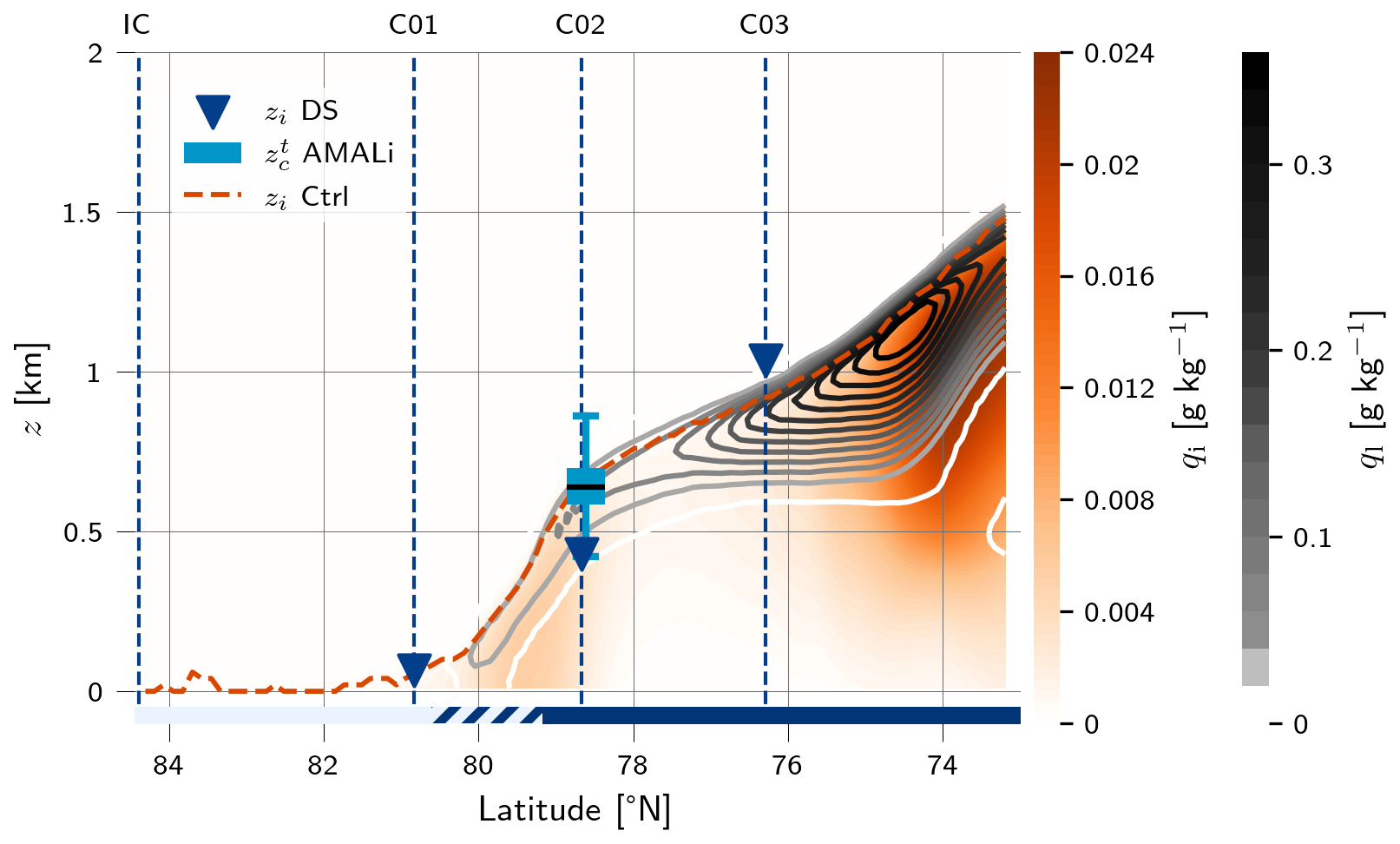
Figure 5 Latitudinal evolution of cloud liquid (grey contour lines) and ice (red filled contours) along the MCAO trajectory. Results from the 45 h semi-Lagrangian DALES simulation Ctrl are shown, including model ABL height (red dashed), compared to dropsonde ABL heights (▾) and cloud-top heights from AMALi lidar aboard the P5 aircraft (light blue boxplot, outliers not shown for better visibility). Dashed vertical lines indicate dropsonde circle locations.

4.2 Temperature and humidity profiles

The vertical structure of virtual potential temperature (ϑ_v) and specific humidity (q) in the Ctrl experiment is evaluated against in-situ observations from HALO dropsondes, closest to the simulation trajectory; the variability of all soundings in each circle is indicated as blue shading in Fig. 6. This comparison reveals possible systematic biases in the thermodynamic state. Figure 6 focuses on the lowest 3 km of the atmosphere to highlight the ABL properties. Above 3 km altitude, the simulation closely follows the observed vertical structure of ϑ_v at all three locations. Larger differences occur for q, primarily due to observed humidity layers not being captured in the smoother simulated humidity structure.

In the region of C01 (Fig. 6a and d), located above sea ice near its edge, an inversion in ϑ_v is detected near the surface at 30 m in the simulation, and at 20 m in the dropsonde profiles, with a thermodynamic wind profile above it. The simulated near surface ϑ_v of −25.6 °C differs by 1.4 K from the dropsonde observations of −24.2 °C and lies within the observed variability. The humidity profiles show greater variability among the dropsondes, with several observed humid layers not captured by the smoother simulated profile; nevertheless, the simulation closely follows the vertical structure of the observed profiles. The near-surface value of q at C01 was 0.5 g km⁻¹ in the simulation and 0.54 g kg⁻¹ in the observations. The close correspondence at C01 reflects the continuous nudging that is active above the ABL top, which is still very low at this stage.

As the air mass moved over the marginal sea ice zone (MIZ) and the open ocean to the location of C02 (Fig. 6b and e), surface warming caused an increase in the near surface air temperature ϑ_v,0 in the simulation of +14.5 K to −11.1 °C, while observed warming was even stronger with a measured increase in ϑ_v,0 of +15.6 K to −8.6 °C. The inversion height was approximately 590 m in both profiles, but the simulated inversion was less steep. Below the inversion, the model shows a cold deviation of 3.3 K, while reproducing the observed mixed-layer structure and inversion height. The increase in evaporation over the open ocean led to an increase in humidity, with surface moisture q₀ of 1.5 g kg⁻¹ in the simulation and 1.6 g kg⁻¹ in the observations. Both show a pronounced drop in humidity near 590 m, with the observed jump being stronger and sharper than the simulation, induced by the prescribed advection of q_t (shown in Fig. 4c). Within the mixed layer, where temperature and humidity are uniform with height, the model underestimates the humidity by an average of 0.2 g g⁻¹. Above the temperature inversion, additional differences result from observed moisture layers that are not captured in the simulation.

Further south, over the open ocean at C03 (Fig. 6c and f), the ABL has deepened further and ϑ_v has continued to increase, with a simulated surface value of ϑ_v,0 of −7.5 °C and an observed value of −4.6 °C representing an underestimation of near-surface warming by 2.9 K. The modelled inversion base is at 830 m, compared to 1000 m in the observations, with the simulated inversion being less steep. Below the temperature inversion, the model underestimates ϑ_v by approximately 2 K. Therefore, there is a consistent cold bias of −2 to −3 K across all circles, a tendency also found by Wendisch et al. (2025) in the limited-area configuration of the ICON model for all observed MCAO cases of HALO–(𝒜𝒞)³ and may reflect uncertainties in the prescribed surface skin temperature and limitations of the bulk surface-flux parametrisation. The humidity in the boundary layer at C03 has also increased further, reaching 1.7 g kg⁻¹ in the simulation and 2 g kg⁻¹ in the observations, with the model underestimating the surface layer of high humidity directly above the ocean. The simulated humidity jump is also weaker than observed. Below the temperature inversion, the model underestimates q by 0.2 g kg⁻¹.

Additional measurements taken with the CMET sonde drifting south along a similar trajectory further support these results. At the same latitude as C01, the CMET flew at an altitude of 340 m at a distance of 225 km to the simulated trajectory. The CMET reached the latitude of interest about 2.5 h later than the simulated air parcel. Here, ${\mathit{\vartheta }}_{\mathrm{v}}=-\text{8.8}$ °C and q=0.52 g kg⁻¹ were measured, which largely corresponds to the simulation in terms of humidity (difference of only 0.02 g kg⁻¹), but with ϑ_v being 5.7 K warmer, which may be due to the proximity to Svalbard and the associated local warming effects. As the trajectory of CMET was closer to Svalbard and travelled through the cloud-free region associated with lee-effects, likely causing a warming of the lower layers. The CMET reached the latitude of C02 7.5 h later at a distance of 132 km from the simulated trajectory. The CMET measured at 902 m above sea level a temperature of ${\mathit{\vartheta }}_{\mathrm{v}}=-\text{1.8}$ °C and q=0.25 g kg⁻¹, which is 3.7 K warmer and 0.2 g kg⁻¹ drier than the simulation. At C03, the CMET was 2 h later and 149 km away from the simulation at an altitude of 1780 m. A virtual potential temperature ϑ_v of 2.7 °C was measured, 1.8 K warmer than in the model and q=0.78 g kg⁻¹, only 0.06 g kg⁻¹ more humid. As the CMET moved south and the influence of Svalbard diminished, the measured air mass increasingly resembled that observed by the dropsondes, with the humidity in all three circles corresponding very closely to the simulated q values measured by the dropsondes.

The overall conclusion from these results is that the LES model reproduces the observed evolution in the vertical thermodynamic structure after C01 to a reasonable degree. This is not trivial, as the nudging takes place above the temperature inversion only, and below it, the simulated ABL is free to evolve. A slight cold and dry bias is evident within the ABL, and the inversions at its top height appear less pronounced than observed. These differences may arise from (i) uncertainties in the surface boundary condition T_skin, and (ii) shortcomings in the bulk flux parametrisation at the surface. Nevertheless, the overall correspondence between simulation and observation indicates that the model adequately reproduces the thermodynamic structure of the observed MCAO, providing a robust basis for further analysis.

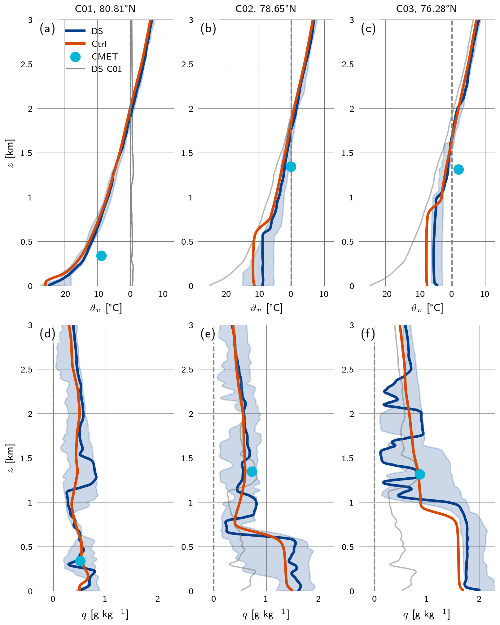
Figure 6 Vertical profiles of virtual potential temperature (ϑ_v) and specific humidity (q). Dropsonde profile (blue) of the dropsonde closest to the simulation trajectory and spread between values measured by 10 sondes per circle (shading); simulation profiles are shown in red. CMET measurements are indicated as blue dots.

4.3 Integrated water paths

The model performance in representing various column-integrated quantities is assessed next. In Fig. 7a, the simulated integrated water vapour (IWV) is evaluated against observations from two sources. The first source are the data from the HAMP radiometer on board HALO which measured along the flight trajectory, and the second is the IWV determined from the dropsonde humidity profiles, averaged over the ten sondes in each circular pattern. The simulation accurately replicated the observed IWV at C01 of 1.9 kg m⁻² with a small difference of 0.1 kg m⁻². At C02, the dropsondes measured 2.7 kg m⁻² IWV, reproduced with +0.04 kg m⁻¹ in the simulation. At C03, the observed IWV was 4.4 kg m⁻², which the simulation slightly overestimated by +0.3 kg m⁻². This temporal evolution of IWV closely follows the HAMP observations, with an RMSE of 0.2 kg m⁻² compared to the simulation. These results suggest that the net input of humidity into the deepening ABL is well captured by the model.

Figure 7b compares the simulated LWP against two measurements. The LWP retrieved from HAMP onboard HALO exhibits a much higher short-term variability than in the simulation, resulting in an RMSE of 30 g m⁻². Despite this, the overall temporal evolution aligns with the simulated LWP, with liquid water strongly increasing after the MIZ. The MiRAC instrument on P5 showed even higher variability due to its high spatial resolution and low flight altitude above the clouds. When averaged, MiRAC observations yield a mean LWP of 0.01 g m⁻², which appears much lower than the simulated LWP of 12 g m⁻², but the simulation value lies within the spread of the LWP observed by MiRAC. These results suggest that, while the observed LWP fluctuates more strongly due to higher resolution, capturing individual cloud streets, than the smoother, domain-average model output, the simulation captures the general trend and magnitude of the evolution of liquid water throughout the event.

The simulated ice water path of all frozen hydrometeors IWP shown in Fig. 7c is only compared to MiRAC measurements aboard P5. The IWP retrievals by HALO were excluded due to large uncertainties for this case. The average observed IWP from MiRAC was 0.6 g m⁻², but similar to the LWP observations, the variability due to the high resolution of individual clouds is large and values range up to 6.2 g m⁻². This high variability may also result from the substantial uncertainties associated with IWP retrievals. The Ze–IWC relationship of Hogan et al. (2006) exhibits uncertainties around a factor of 2, caused by the strong temperature dependence of ice particle size distributions and densities. At warmer temperatures, the ice water content IWC tends to be overestimated, whereas at colder temperatures it is generally underestimated. This temperature sensitivity is particularly relevant for 94 GHz radar, where Mie-scattering further increases the retrieval uncertainty. Compared to the simulated IWP in the location of the P5 measurements of 2.58 g m⁻², an RMSE of 73.34 g m⁻² is found. It should also be noted that the P5 observations do not coincide with the air mass trajectory but were collected at a later time, limiting the comparability of the data (Fig. 1). A notable feature of the latitudinal evolution of the simulated IWP is the local maximum reached in the simulation just before C02; the realism cannot be verified due to the absence of reliable IWP measurements along the whole trajectory.

4.4 Surface heat fluxes

The surface heat fluxes are key drivers of ABL evolution in MCAOs. To evaluate the simulated sensible (H) and latent (E) heat fluxes, we estimate these data from dropsonde observations following the thermodynamic method suggested by Hartmann et al. (1997). This method assumes steady-state conditions, negligible radiative divergence and cross-flow advection, and minimal entrainment above the mixed layer. Here, following Hartmann et al. (1997), the steady-state assumption allows thermodynamic differences between successive downstream profiles to be interpreted as along-flow advective changes and linked to the vertically integrated surface heat and moisture input. Then, the sensible and latent heat energy fluxes can be calculated as

$$\begin{array}{}\text{(6)}& H_{\mathrm{DS}}=\mathit{\varrho }\cdot c_{\mathrm{p}}\cdot u_{\mathrm{ML}}\underset{z_i}{\overset{\mathrm{0}}{\int }}{\displaystyle \frac{\mathrm{\Delta }\mathit{\vartheta }}{-\mathrm{\Delta }y}}\mathrm{d}z-H_{\text{C}},\end{array}$$

$$\begin{array}{}\text{(7)}& E_{\mathrm{DS}}=\mathit{\varrho }\cdot L_{\mathrm{v}}\cdot u_{\mathrm{ML}}\underset{z_i}{\overset{\mathrm{0}}{\int }}{\displaystyle \frac{\mathrm{\Delta }q}{-\mathrm{\Delta }y}}\mathrm{d}z+H_{\text{C}},\end{array}$$

where ϱ represents the air density, c_p the specific heat capacity, L_v the latent heat of evaporation, u_ML the mean horizontal wind speed within the mixed layer and z_i the height of the ABL. Δy is the horizontal distance between two profiles. The contribution of condensational heating within the cloud layer is represented by the following formulas:

$$\begin{array}{}\text{(8)}& H_{\mathrm{C}}=\mathit{\varrho }\cdot L_{\mathrm{v}}\cdot u_{\mathrm{ML}}\underset{z_i}{\overset{z_{\mathrm{b}}}{\int }}{\displaystyle \frac{\mathrm{\Delta }l}{-\mathrm{\Delta }y}}\mathrm{d}z,\end{array}$$

where z_b represents the height of the cloud base, defined as the lowest altitude at which the relative humidity reaches saturation with respect to the ice or liquid. Meanwhile, Δl refers to the difference in q_l between the profiles, which is approximated as the upper limit of q_l within the cloud layer. This is estimated as the difference of q_t within the cloud and the average $\stackrel{\mathrm{‾}}{q_{\text{t,BC}}}$ below the cloud layer, following Hartmann et al. (1997). In the model, the surface heat fluxes can be sampled continuously as

$$\begin{array}{}\text{(9)}& {\displaystyle }{H}_{\text{Ctrl}}& {\displaystyle }=\mathit{\varrho }\cdot c_{\mathrm{p}}\cdot \stackrel{\mathrm{‾}}{w^{\prime }\cdot {\mathit{\vartheta }}^{\prime }},\text{(10)}& {\displaystyle }{E}_{\text{Ctrl}}& {\displaystyle }=\mathit{\varrho }\cdot L_{\mathrm{v}}\cdot \stackrel{\mathrm{‾}}{w^{\prime }\cdot q^{\prime }},\end{array}$$

with $\stackrel{\mathrm{‾}}{w^{\prime }{\mathit{\vartheta }}^{\prime }}$ and $\stackrel{\mathrm{‾}}{w^{\prime }{q}^{\prime }}$ representing the turbulent kinematic fluxes of temperature and moisture at the surface.

The simulation produced H_Ctrl values up to 830 W m⁻² and E_Ctrl values up to 102 W m⁻² over the open ocean. In particular, the sensible heat flux is substantially higher than the climatological mean sensible flux of about 200 W m⁻² during MCAOs, while the latent heat flux is comparable to the climatological mean latent heat flux of 100 W m⁻² reported by Papritz and Spengler (2017) for MCAOs in the region west of Svalbard. The difference in potential temperature between the near-surface atmosphere and the ocean surface causes a direct response in the sensible heat flux, while the latent heat flux is limited by the saturation specific humidity at the sea surface temperature (Papritz et al., 2015; Papritz and Spengler, 2017). In the observed region, H was generally more efficient than E in extracting energy from the ocean surface, but the relative importance of E increased as the air is mass advected away from the sea-ice edge over warmer waters. South of 75° N, the mean values of H_Ctrl and E_Ctrl were 69 and 17 W m⁻², respectively, consistent with the findings of Brümmer (1997).

Dropsonde-derived H_DS values considerably underestimate simulated surface sensible heat fluxes by 564 W m⁻² between C01 and C02 and 306 W m⁻² between C02 and C03. We speculate that this offset is mostly due to numerous assumptions in the method of deriving fluxes from observed profiles. To improve comparability between model and measurements and gain further insight, the same diagnostic technique is applied to the simulated profiles (Fig. 6), yielding much better agreement. The associated RMSE between H_DS and H_{Ctrl, Prof} is 95 W m⁻². Between C02 and C03, the thermodynamic method yields a simulated value of only H_{Ctrl, Prof}=21 W m⁻², compared to H_DS=170 W m⁻², largely underestimating the surface sensible heat flux. Note that the dropsonde-derived E_DS in the marginal ice zone (C01–C02) is very small (2.6 W m⁻²) compared to the simulated fluxes that exceeded 100 W m⁻², but increased to 16 W m⁻² between C02 and C03, closer to the simulated values. The RMSE of 8.9 W m⁻² between E_DS and E_{Ctrl, Prof} indicates that although the observational profile-based method struggles to fully capture the true flux magnitudes in the early MCAO phase, it reproduces their relative variability well when applied consistently.

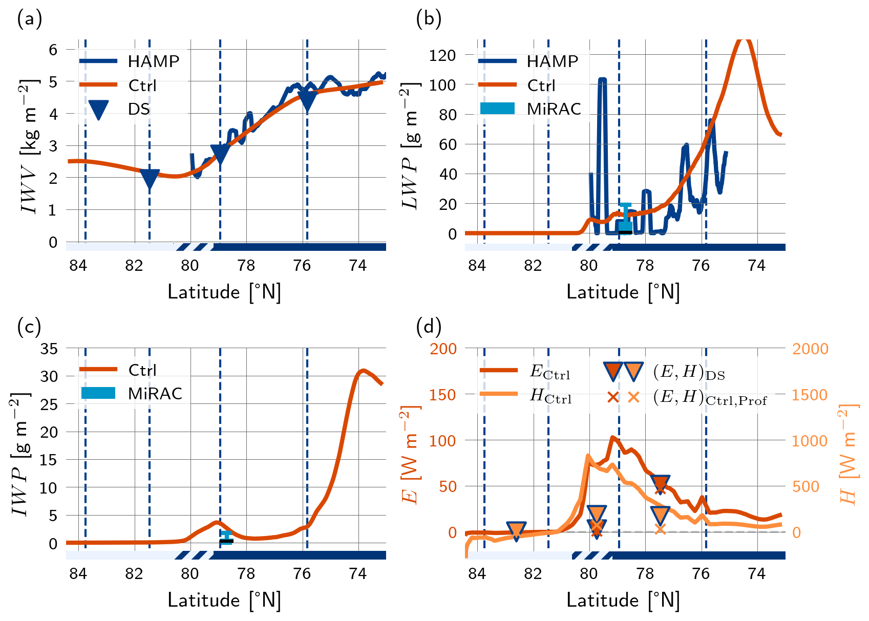
Figure 7 Latitudinal evolution of various bulk properties of the simulated MCAO in the Ctrl experiment. (a) Integrated water vapour IWV simulation (red line) compared to longitudinally averaged observations from HALO (blue line) and estimates based on dropsonde data (▾). (b) Simulated liquid water path LWP and (c) ice water path IWP (red lines) compared to HALO (dark blue line) and P5 (light blue boxplot, outliers not shown for better visibility) observations. (d) Simulated surface latent (E, red line) and sensible (H, yellow line) heat fluxes compared to estimates based on dropsonde data following the method of Hartmann et al. (1997) (▾). The same method applied to model profiles is also shown, for reference (×). In all figures, the vertical dashed lines mark the location of the dropsonde circles. The coloured bar at the bottom indicates sea ice (sic >0.9, light blue), marginal sea-ice ($\text{0}<\mathrm{sic}\le \text{0.9}$, hatched), and open ocean (sic =0, dark blue).

5 Results II: Subsidence impacts

The results discussed so far indicate that the Ctrl simulation reproduces the temporal evolution of the ABL well, including various water paths and surface energy fluxes. Therefore, the Ctrl experiment represents a robust and realistic foundation for subsequent Lagrangian LES sensitivity experiments, as applied in this section to investigate the impact of mesoscale subsidence on the ABL and cloud evolution. In total, five experiments with differing mesoscale subsidence are performed and analysed. As described in Sect. 3.4, four additional experiments were conducted with the Ctrl subsidence field multiplied by a factor $\mathit{\{}\mathrm{0},\mathrm{0.1},\mathrm{0.5},\mathrm{2.0}\mathit{\}}$, respectively.

5.1 Sensitivity analysis

Figure 8 shows the evolution of q_l and q_i along the MCAO trajectory. In the no-subsidence (NoSub) setup, the cloudy ABL deepens the fastest, approaching the parabolic deepening rate ($\sim t^{\mathrm{1}/\mathrm{2}}$) after the air mass moves over the open ocean (Stevens, 2007). In this setup, the cloud mass is the largest, both in liquid and frozen form. The higher the prescribed subsidence forcing, the more the ABL deepening driven by turbulent/convective entrainment is suppressed by subsidence. This in particular applies during the time period between C02 and C03, where the observed low-level subsidence has its maximum (Fig. 4a). This leads to the development of thinner clouds and less q_l and q_i. In the Sub200 case, only a very thin, shallow mixed-phase cloud is observed.

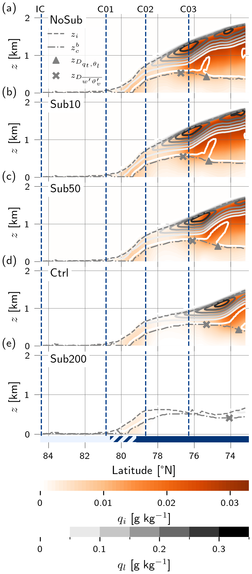
Figure 8 Latitudinal evolution of cloud liquid (grey) and ice (red) along the MCAO trajectory for all sensitivity experiments. Dashed horizontal lines indicate dropsonde circle locations. Boundary layer height z_i and cloud base z_b are indicated by grey dashed and dot-dashed lines, respectively. The markers × and ▴ indicate decoupling points and heights with respect to $\stackrel{\mathrm{‾}}{w^{\prime }{\mathit{\vartheta }}_{\mathrm{v}}^{\prime }}$ and Δq_t and Δϑ_l respectively (Sect. 5.2 for definition). The coloured bar at the bottom indicates sea ice (sic >0.9, light blue), marginal sea-ice ($\text{0}<\mathrm{sic}\le \text{0.9}$, hatched), and open ocean (sic =0, dark blue).

To gain more insight into the spatial structure of the cloud field, Fig. 9 presents horizontal cross-sections of q_l and q_i through the centre of the simulated domain for all five simulations. These locations are sampled at regular intervals along the trajectory, beginning at C01 near the sea-ice edge and extending southward to 73.25° N at the end of the simulation period. The grey shading highlights regions in which the cloud layer is decoupled from the surface, following the criterion of Jones et al. (2011). This diagnostic is defined by the thresholds $\mathrm{\Delta }{q}_{\mathrm{t}}={\stackrel{\mathrm{‾}}{q}}_{t,\text{bot}}-{\stackrel{\mathrm{‾}}{q}}_{t,\text{top}}>\text{0.5}$ g kg⁻¹, based on the layer-mean total-water mixing ratio in the upper and lower 25 % of the boundary layer, and $\mathrm{\Delta }{\mathit{\vartheta }}_{\mathrm{l}}={\stackrel{\mathrm{‾}}{\mathit{\vartheta }}}_{\text{l,top}}-{\stackrel{\mathrm{‾}}{\mathit{\vartheta }}}_{\text{l,bot}}>\text{0.5}$ K, calculated analogously for the layer-mean liquid-water potential temperature. These metrics have been associated with the onset of boundary-layer decoupling and the subsequent transition from roll convection to open-cell structures in MCAOs (Karalis et al., 2022; Abel et al., 2017). What stands out during the decoupled phase is the presence of liquid-phase shallow cumulus clouds, rising into the capping mixed-phase cloud layer.

Across the simulations, the onset of decoupling exhibits a systematic dependence on the prescribed subsidence: in cases with reduced subsidence, the decoupling occurs closer to the sea-ice edge and is accompanied by overall larger maxima in both liquid and ice water content. While all simulations show the initial formation of a thin ice cloud at C01, substantial differences arise beginning at C02, most notably in cloud-top height and the vertical distribution of liquid and ice. The Sub200 simulation produces only a shallow ice cloud capped by a thin liquid layer, with little variation in cloud-top altitude throughout the trajectory. In contrast, the simulations with weaker subsidence develop considerably deeper clouds, characterised by more complex internal structure and enhanced condensate mass.

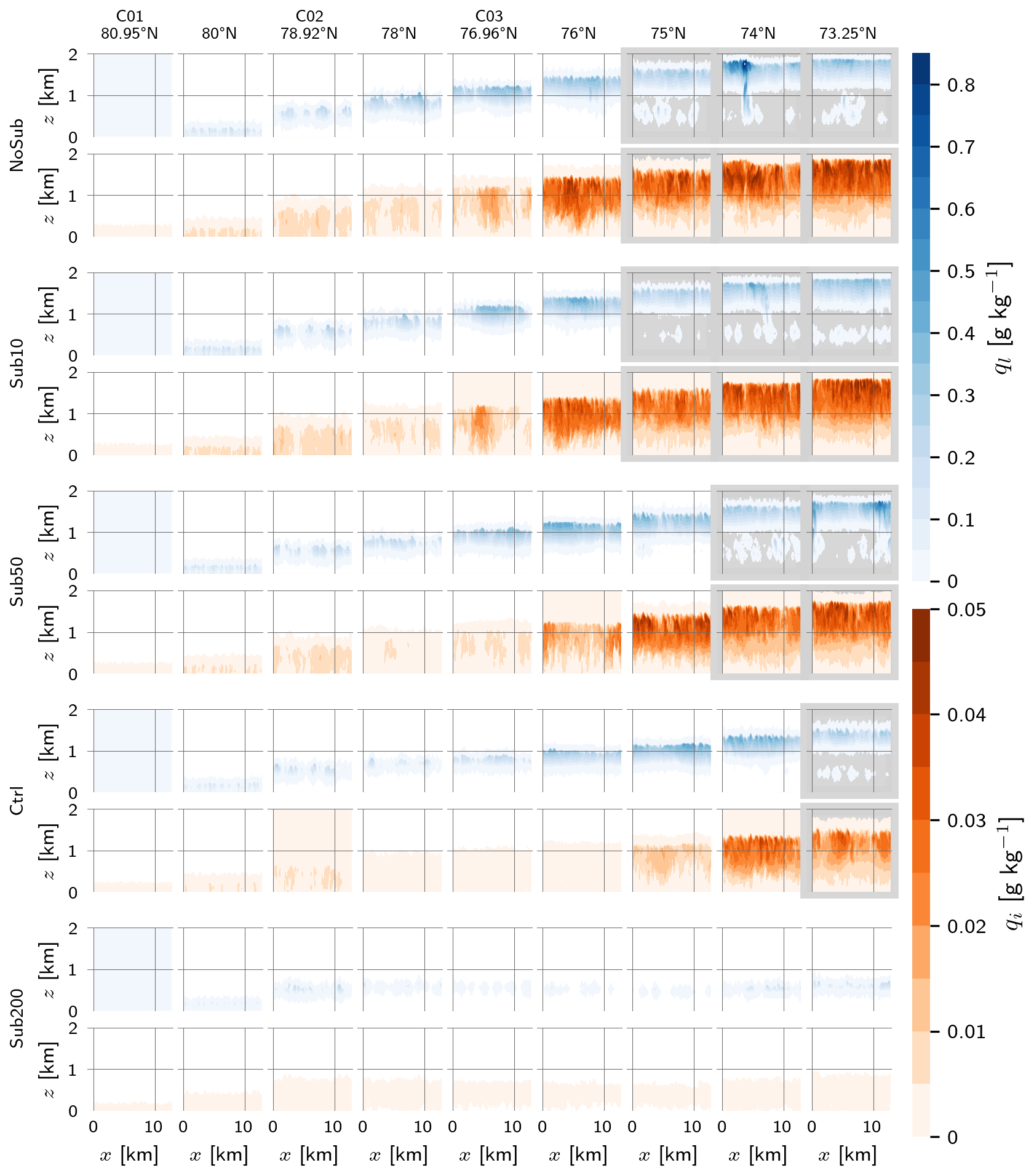
Figure 9 Horizontal cross-sections of cloud liquid water (q_l) and cloud ice (q_i) at the domain centre (y=6.4 km), at different locations along the trajectory and for different subsidence experiments. Cross-sections of decoupled clouds (Δq_t>0.5 g kg⁻¹ and Δϑ_l>0.5 K) are highlighted in grey.

The impact of subsidence on the developing ABL is characterised by various bulk quantities, as shown in Fig. 10. The integrated water vapour IWV (Fig. 10a) is similar in all simulations, but the boundary layer (Fig. 10d) in the NoSub case reaches substantially greater depths (2 km), following a parabolic deepening rate due to unimpeded entrainment at the ABL top. All simulations exhibit a similar strong initial boundary layer growth within the MIZ and immediately downstream of the sea ice edge (up to C02), driven primarily by intense surface heat fluxes in this region (Fig. 7). However, after this initial phase, the Sub200 simulation boundary layer actually becomes shallower, with the strong subsidence keeping z_i below 1 km. In contrast, the Ctrl, Sub50, and Sub10 simulations all maintain continued ABL deepening, though z_i remains below the parabolic limit visible in NoSub.

The liquid water path LWP (Fig. 10c) exhibits an initial peak near the sea ice in all simulations, coinciding with the region of strong boundary layer growth at approximately 80° N on average. The RMSE in the location of the peak between the simulations is 0.01° N, and the strength of the peak decreases with increasing subsidence by 18 g m⁻², with an overall RMSE of 4.9 g m⁻². A second, more pronounced LWP maximum occurs later at 76.3° N in NoSub, with a maximum value of 173 g m⁻². For Sub50 and Ctrl, this secondary peak shifts to lower latitudes and reduced magnitudes, occurring at 76° N (167 g m⁻²) and 74.4° N (133 g m⁻²), respectively. In Sub200, the liquid water path does not recover after the initial maximum and shows only a gradual increase later in the simulation, beyond 74° N.

The ice water path IWP (Fig. 10e), including all frozen hydrometeors, displays a similar spatial evolution, with an initial peak forming in the MIZ around 79.4° N, consistent in all simulations. Subsequently, IWP increases over the open ocean following the sea ice edge. Compared to LWP the ice growth begins slightly earlier (also visible in Fig. 9), which is consistent with previous studies of Arctic MCAOs (Murray-Watson and Gryspeerdt, 2024; Inoue et al., 2021). The peak IWP in NoSub occurs at 75.7° N with 48 g m⁻², whereas for Sub50 and Ctrl it shifts to 75.7 and 73.8° N respectively with reduced magnitudes of 41 and 31 g m⁻² respectively. The Sub200 simulation exhibits no such shift or comparable peak values, indicating a systematic suppression of ice growth under stronger subsidence.

The ratio of ice to liquid water, $\frac{\mathrm{IWP}}{\mathrm{LWP}}$, calculated only for regions with a significant liquid content (LWP> 1 g m⁻²), highlights these differences more clearly (Fig. 10b). The initial shallow cloud developing above the MIZ shows a similar structure among NoSub, Sub10, Sub50, and Ctrl, while Sub200 displays a slightly larger ice fraction in the initial cloud. However, because of the overall thinness of both liquid and ice layers, this difference cannot be regarded statistically significant. In later stages, LWP in Sub200 falls below 1 g m⁻², producing a discontinuity in the $\frac{\mathrm{IWP}}{\mathrm{LWP}}$ ratio, while in the remaining cases a clear shift towards later growth of IWP is evident.

Finally, the impact of subsidence on the total surface precipitation rate (P_tot) (Fig. 10f) is broadly similar to the IWP. The NoSub simulation reaches precipitation rates up to 60 mm h⁻¹ towards the end of the simulation, compared with 25 mm h⁻¹ at the peak near 74° N for Ctrl. In Sub200, precipitation remains confined to the initial shallow cloud phase, with maximum rates of only 2.1 mm h⁻¹.

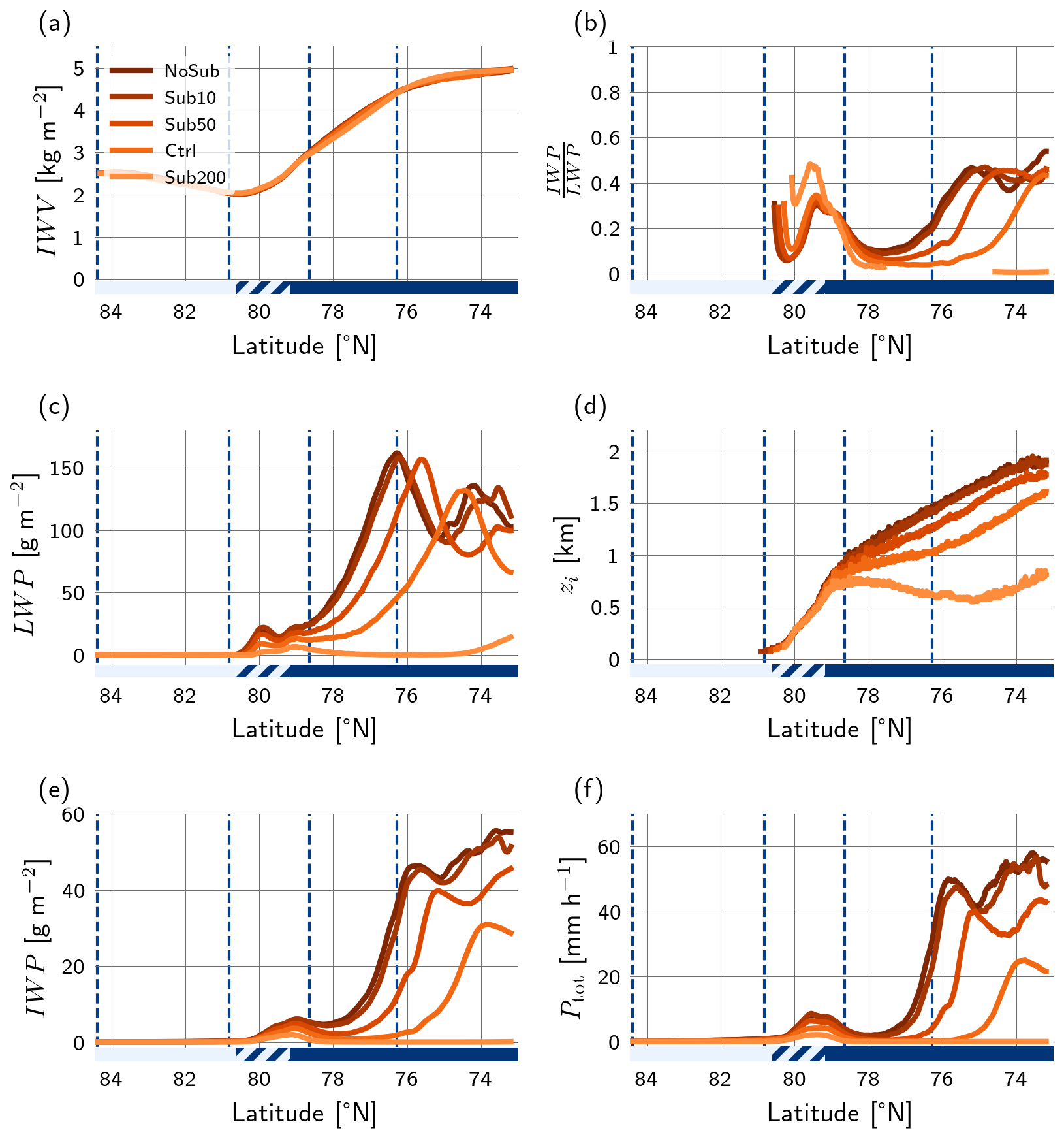
Figure 10 Integrated water vapour IWV (a), liquid water path LWP (c), ice water path IWP (e), including all frozen hydrometeors, together with its ratio $\frac{\mathrm{IWP}}{\mathrm{LWP}}$ (b), the boundary layer height z_i (d) and the total precipitation rate P_tot (e) for Lagrangian LES with different subsidence forcings. The locations of the dropsonde circles are shown as vertical dashed lines, and the surface cover is indicated as sea ice (sic >0.9, light blue), marginal sea-ice zone (0<sic≤0.9, hatched), and open ocean (sic =0, dark blue).

5.2 Glaciation and decoupling

The results so far indicate that the behaviour of the cloud ice phase is particularly affected by the strength of subsidence. To gain further insight, the relative contributions by the three frozen hydrometeor classes in the LES microphysical scheme are investigated. The integrated column water paths of cloud ice (CIWP), snow (SIWP), and graupel (GIWP) are shown in Fig. 11. The behaviour of CIWP (Fig. 11a) closely follows that of the total ice water path (IWP), reflecting its dominant contribution to the total ice mass. The maximum values of CIWP reach 38 g m⁻² at 73.4° N for NoSub and 32 g m⁻² at 73.7° N for Ctrl, with a systematic decrease in amplitude under stronger subsidence. The SIWP (Fig. 11c) distribution exhibits a similar latitudinal progression, with peak values occurring later and at reduced magnitudes as subsidence increases. However, unlike CIWP, SIWP does not sharply decline after the peak but plateaus afterwards, reaching 9.6 g m⁻² at 73.3° N for NoSub and 5.5 g m⁻² at 73.4° N for Ctrl. The graupel path GIWP (Fig. 11b) exhibits the most distinct and localised peak. In NoSub the peak occurs at 76° N with a magnitude of 8.4 g m⁻², generally shifting southward with increasing subsidence to 74° N for Ctrl, weakening in amplitude to 2.7 g m⁻². The Sub200 experiment does not develop graupel. In this southward progression, the width of the graupel peak remains similar.

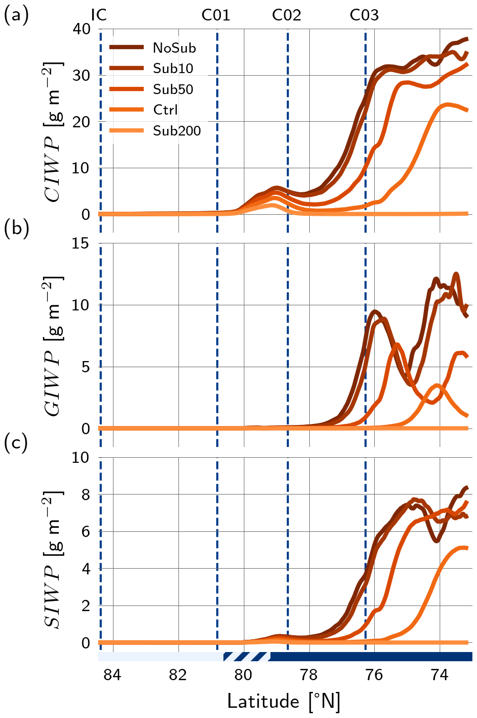
Figure 11 Integrated cloud ice water path CIWP (a), integrated snow water path SIWP (c) and integrated graupel water path GIWP (b). The locations of the dropsonde circles are shown as vertical dashed lines, and the surface cover is indicated as sea ice (sic >0.9, light blue), marginal sea-ice zone ($\text{0}<\mathrm{sic}\le \text{0.9}$, hatched), and open ocean (sic =0, dark blue).

Graupel is typically formed in convective updrafts, as it requires substantial vertical velocities. Accordingly, the southward shift and progressive weakening of the peak in GIWP with increasing subsidence probably reflects a similar shift in convective dynamics. This motivates a deeper investigation of the behaviour of boundary-layer internal decoupling. Previous MCAOs studies have established that such decoupling plays a central role in the transition from organised roll convection to open-cellular convection. Enhanced precipitation, often driven by secondary ice production and riming, has been shown to promote evaporation and sublimation below the cloud, thereby cooling and moistening the sub-cloud layer. This preconditioning in water vapour at lower levels accelerates the breakup of stratocumulus decks and favours the onset of cellular convection. As a result, the surface supply of moisture and heat to the cloud layer is reduced, weakening roll structures and promoting the development of cellular patterns (Abel et al., 2017; Tornow et al., 2021; Karalis et al., 2022; Wu et al., 2025). A slightly different form of decoupling that does not involve precipitation has been proposed earlier by Bretherton and Wyant (1997), showing that during deepening marine subtropical stratocumulus-topped ABLs a layer of negative buoyancy flux $\stackrel{\mathrm{‾}}{w^{\prime }{\mathit{\vartheta }}_{\mathrm{v}}^{\prime }}$ can form below cloud base, as a result of top-down and bottom-up driven mixing becoming too far separated in the vertical. This negative buoyancy flux layer then disrupts the ABL-deep circulation, inducing decoupling. The latitudinal development of the buoyancy flux is shown in Fig. D1.

Both mechanisms of decoupling and the link to graupel formation are investigated next. The buoyancy-based decoupling mechanism is assessed by defining a decoupling point $D_{\stackrel{\mathrm{‾}}{w^{\prime }{\mathit{\vartheta }}_{\mathrm{v}}^{\prime }}}$ as the time point at which $\stackrel{\mathrm{‾}}{w^{\prime }{\mathit{\vartheta }}_{\mathrm{v}}^{\prime }}$ becomes negative below cloud base for the first time, and remains so until the end of the simulation (indicated as ▾ in Fig. 8). The humidity-based decoupling mechanism involving precipitation evaporation is assessed by defining a second decoupling point, this time inferred from Δq_t and Δϑ_l denoted $D_{q_{\mathrm{t}},{\mathit{\vartheta }}_{\mathrm{l}}}$, as discussed above (Sect. 5.1). Comparing these two definitions gives insight into how exactly decoupling works in MCAOs and how it affects the shifts in ice phase hydrometeors.

Figure 12 compares the locations of the largest peaks in liquid water path (LWP_max), graupel water path (GIWP_max), and surface precipitation rate (P_{tot, max}) with the two decoupling points $D_{q_{\mathrm{t}},{\mathit{\vartheta }}_{\mathrm{l}}}$ and $D_{\stackrel{\mathrm{‾}}{w^{\prime }{\mathit{\vartheta }}_{\mathrm{v}}^{\prime }}}$, for all simulations except Sub200 (in which no graupel appears). A key result that stands out is that buoyancy-based decoupling (vertical axis) structurally happens first, in all simulations (also indicated in Fig. 8). This is followed by the peak in LWP, then integrated graupel, then surface precipitation, and finally the precipitation-based decoupling point. This sequence of events typically covers 1° of latitude in this MCAO case, and shifts southward with increasing prescribed mesoscale subsidence. The order of appearance of the various maxima is consistent with the idea that (i) internal buoyancy-decoupling initiates events and causes stronger surface-driven convection, (ii) driving stronger precipitation formation (mainly in graupel form) that efficiently depletes cloud liquid water mass (as discussed by Abel et al., 2017), (iii) forming intense graupel for a while, (iv) associated with enhanced surface precipitation which then (v) further stabilises the lower boundary layer through evaporation below cloud base, suppressing vertical mixing and further enhancing decoupling (Wu et al., 2025). The last step is also suggested by the slight lowering of liquid cloud base height visible in Fig. 8. This sequence of events ultimately yields a fully decoupled structure with respect to Δq_t and Δϑ_l at $D_{q_{\mathrm{t}},{\mathit{\vartheta }}_{\mathrm{l}}}$.

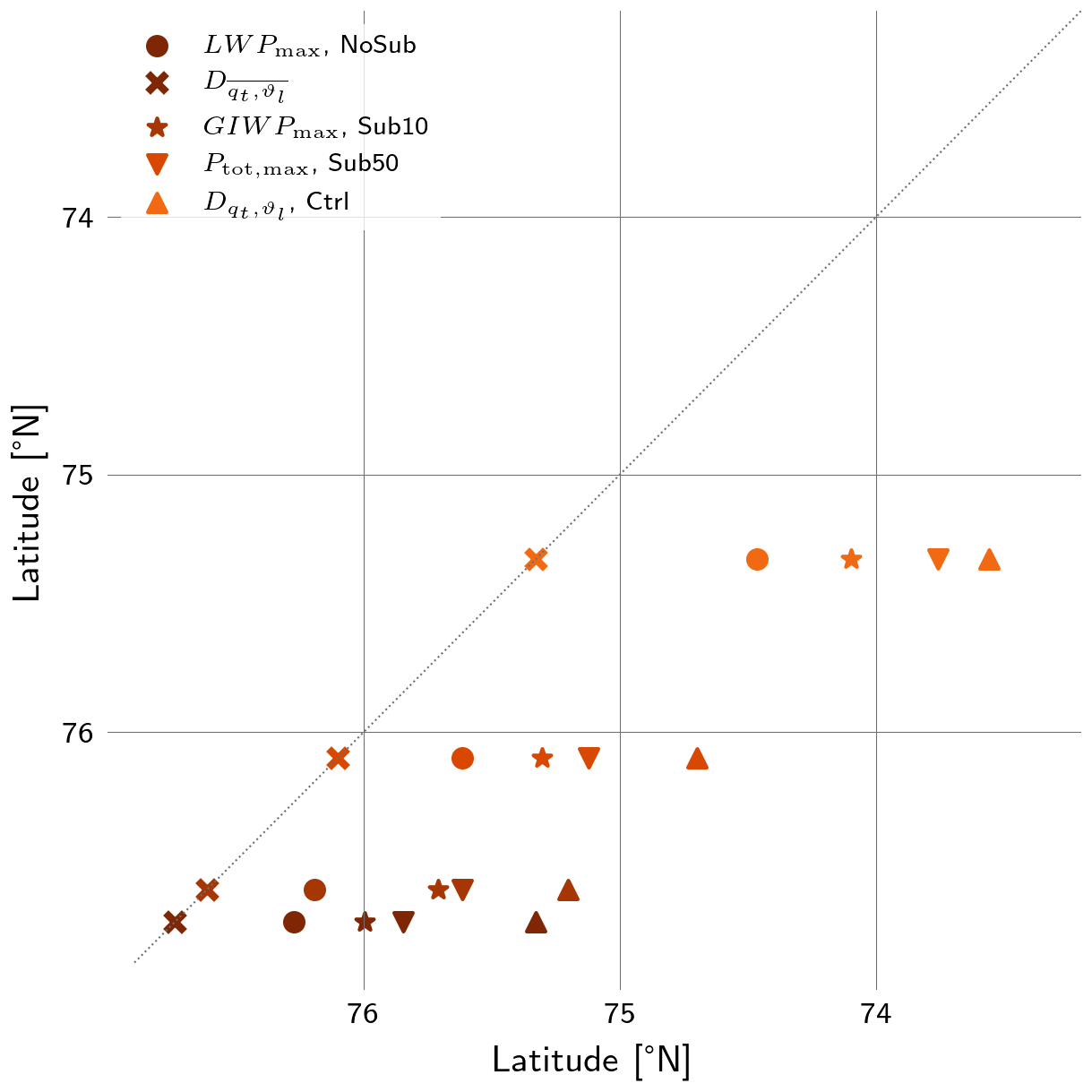
Figure 12 Location of the largest peak in liquid water path LWP_max, graupel water path GIWP_max and precipitation P_{tot, max} and the location of decoupling with respect to the q_t and ϑ_l profiles $D_{q_{\mathrm{t}},{\mathit{\vartheta }}_{\mathrm{l}}}$ (following Jones et al., 2011) in relation to the location of decoupling with respect to the buoyancy flux $D_{\stackrel{\mathrm{‾}}{w^{\prime }{\mathit{\vartheta }}_{\mathrm{v}}^{\prime }}}$ (following Bretherton and Wyant, 1997). The colours represent the different simulation experiments as in Fig. 11.

6 Discussion

The sensitivity experiments suggest that the influence of subsidence extends beyond a simple control on boundary layer height. Previous observational and modelling studies have demonstrated that large-scale subsidence influences the evolution of Arctic marine cold air outbreaks by modifying inversion strength, cloud-top height, and the thermodynamic structure of the boundary layer (Brümmer, 1997; McCoy et al., 2017; Young et al., 2018; Schirmacher et al., 2024). However, the exact causal connection between these features and processes including cloud glaciation and boundary layer decoupling has remained less clear. The results obtained in this study provide further insight, suggesting that larger-scale subsidence can act as a strong control on the entire transition of the atmospheric boundary layer and clouds. While the boundary layer evolution under such imposed subsidence involves various small-scale processes that could be described individually, we find that it makes much more sense to interpret them in combination, as they act as a sequence of strongly connected processes. This sequence was consistently diagnosed in all simulations carried out in this study.

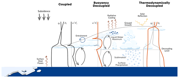
Figure 13 conceptually summarizes the sequence of processes. Initially, the boundary layer is fully coupled to the ocean surface. Strong sensible heat fluxes maintain turbulent mixing throughout the boundary layer, resulting in nearly vertically homogeneous profiles of liquid water potential temperature and total water mixing ratio. Such coupled boundary layers are characteristic of the early stages of marine cold air outbreaks, where large surface-atmosphere temperature contrasts generate vigorous turbulence and rapid boundary layer growth (Brümmer, 1997; Fletcher et al., 2016; Dahlke et al., 2022). During this stage, cloud evolution is primarily governed by the interaction between surface fluxes, entrainment-deepening and cloud-top radiative cooling, processes that have long been recognised as essential for maintaining Arctic mixed-phase stratocumulus (e.g. Morrison et al., 2012; Neggers et al., 2019). During this phase, subsidence primarily controls the rate at which the boundary layer can deepen by opposing entrainment at the inversion.

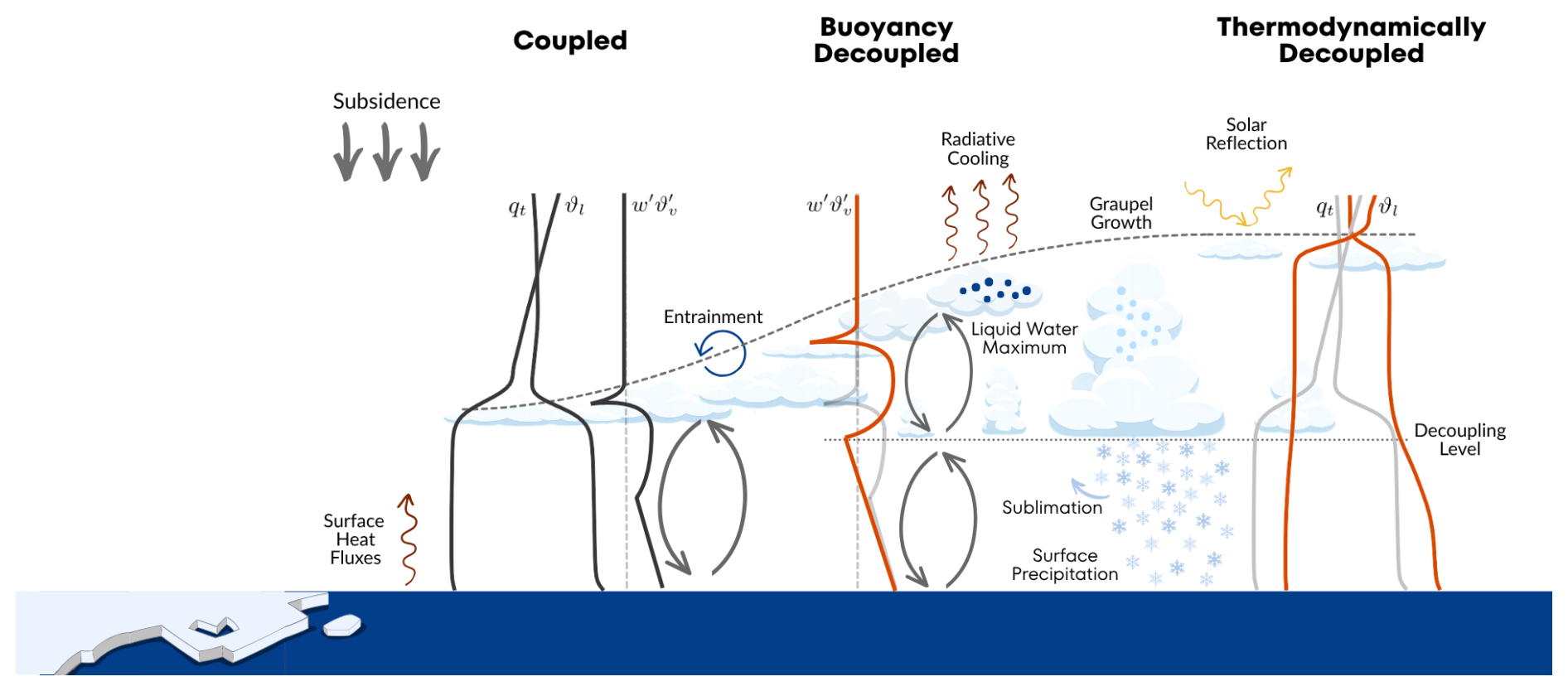
Figure 13 Conceptual evolution of the atmospheric boundary layer during the modelled Arctic marine cold air outbreak. Black and grey profiles of liquid water potential temperature ϑ_l, total humidity q_t and buoyancy flux $w^{\prime }{\mathit{\vartheta }}_{\mathrm{v}}^{\prime }$ indicate a coupled boundary layer, whereas the orange profiles illustrate decoupling with respect to buoyancy-based ($w^{\prime }{\mathit{\vartheta }}_{\mathrm{v}}^{\prime }$) and thermodynamic (ϑ_l, q_t). The top of the boundary layer is indicated as a dashed line.

Sustained entrainment deepening, driven by superimposed bottom-up (surface buoyancy flux) and top-down (cloud-top radiative cooling) processes (Wyngaard and Brost, 1984), at some point leads to boundary-layer internal decoupling. We find that this internal decoupling is first visible in the negative buoyancy flux that develops below cloud base, with liquid water potential temperature and total humidity still remaining relatively well mixed at this stage. This buoyancy-driven decoupling therefore represents the earliest stage of the transition, acting as a precursor to thermodynamic separation of the cloud and sub-cloud layer that is known to develop at a later stage (Abel et al., 2017). To our knowledge, such buoyancy flux decoupling has not been previously been identified during Arctic marine cold air outbreaks.

At this point it is instructive to draw some parallels with warm stratocumulus-to-cumulus transitions in the marine subtropics, which have been intensely studied for decades (Bretherton and Pincus, 1995; Bretherton et al., 1995; Wood and Bretherton, 2004; van der Dussen et al., 2013; Neggers et al., 2017). As outlined in the key study by Bretherton and Wyant (1997), internal decoupling in the buoyancy flux profile in a deepening well-mixed boundary layer can initiate as a result of the top-down and bottom-up driven turbulent circulations failing to fully overlap. We find that the same happens in MCAOs, triggering the formation of cumulus clouds with their base at the decoupling level (visible in Fig. 9). However, rather than resulting in a warm shallow-cumulus regime and eventual stratocumulus breakup, the transition proceeds towards a decoupled system that includes mixed-phase clouds. Ice microphysical processes such as ice growth, riming, graupel formation, and sub-cloud sublimation then become central to the subsequent cloud transition. These aspects represent defining differences with the warm subtropics.

Following this initial decoupling, the cloud layer continues to deepen while the upper and lower parts of the boundary layer become increasingly isolated from each other. During this stage the simulations exhibit a maximum in liquid water path before ice production and graupel formation become effective. This evolution is consistent with the established understanding of mixed-phase cloud microphysics, in which increasing liquid water availability promotes depositional ice growth through the Wegener–Bergeron–Findeisen process before riming becomes increasingly important and eventually produces graupel (Morrison et al., 2012; Young et al., 2018; Eirund et al., 2019). Enhanced graupel formation subsequently increases precipitation, removing condensate from the cloud layer and reducing cloud liquid water through collection and sedimentation. At the same time, sublimation below cloud base cools and moistens the sub-cloud layer, while reduced turbulent exchange strengthens the vertical gradients in liquid water potential temperature and moisture. Together these processes ultimately produce a fully thermodynamically decoupled boundary layer.

This particular sequence of processes, starting with buoyancy decoupling and defined by the set of markers as shown in Fig. 12, occurred in every experiment conducted in this study. However, the imposed subsidence strength strongly affects its timing. Reduced subsidence allows more rapid boundary layer deepening, resulting in earlier buoyancy-driven decoupling, larger liquid water paths, enhanced convective overturning and stronger graupel formation. Conversely, stronger subsidence suppresses boundary layer deepening, delays the onset of decoupling and substantially reduces cloud glaciation. These results are in principle consistent with previous idealised and high-resolution simulations of Arctic cloud systems (Young et al., 2018; Neggers et al., 2019). This study provides more insight into these responses. A key outcome is that processes such as cloud glaciation and boundary layer decoupling do not act independently, but strongly interact and are part of the ongoing adjustment of the newly formed marine boundary layer to the changed external conditions after leaving the sea ice edge. Subsidence does not directly determine the microphysical evolution of the cloud, but modifies the boundary layer structure in which these processes occur. By controlling boundary layer deepening and decoupling, subsidence indirectly regulates the timing of cloud deepening, mixed-phase cloud development, precipitation formation and the transition towards a thermodynamically decoupled boundary layer.

The precise timing of cloud transitions during MCAOs thus depends on the environmental conditions encountered by the air mass. Factors such as the surface-air temperature difference, aerosol conditions and the effective strength of radiative cooling can all affect the exact onset of decoupling and subsequent cloud glaciation (Eirund et al., 2019; Tornow et al., 2021; Chylik et al., 2023). Additional sensitivity experiments using the same model setup indicate that the ice-phase pathway is sensitive to CCN concentrations, with higher CCN concentrations shifting ice precipitation from graupel toward snow (not shown). This suggests that the timing and partitioning of precipitating ice depend on the microphysical representation, including processes that control droplet size and riming, as well as on prescribed aerosol concentrations. A more systematic investigation of these sensitivities would be required to assess their impact on the processes identified in this study. In addition, local variations in the larger-scale subsidence field may similarly influence precipitation timing, including through lee-side effects associated with local orography. But the conceptual model shown in Fig. 13 does include all key processes found in this study to govern the cloud evolution during Arctic MCAOs. It might thus be useful as a physically consistent framework of reference for interpreting cloud transitions during both observed and modelled MCAO events.

7 Conclusions

This study investigates the sensitivity of Arctic mixed-phase cloud evolution in marine cold air outbreaks with respect to mesoscale subsidence. A Lagrangian Large-Eddy Simulation framework constrained by observations obtained during the airborne HALO–(𝒜𝒞)³. The control simulation was evaluated against the extensive and independent set of airborne in-situ and remote-sensing and meteorological balloon measurements. In the control run, the model reproduced the vertical thermodynamic structure of the observed marine cold air outbreak within the range given by the measurement uncertainties, capturing the evolution of air temperature, humidity, and ABL height along the Lagrangian trajectory. Compared to dropsonde, radiometer, and lidar data, the control simulation accurately represented the integrated water vapour and liquid water path, with a slight cold and dry bias at lower levels. The general agreement between control run results and the corresponding measurements demonstrates that the applied forcing and initialisation derived from the HALO–(𝒜𝒞)³ measurements provide a robust foundation for reproducing the dynamics and properties of the Arctic atmospheric boundary layer, and underscores the importance of constraining simulations with detailed observations.

Sensitivity experiments with the tested large-eddy simulation model revealed that subsidence exerts a strong control on the depth of the atmospheric boundary layer, the height of the cloud top, and the partitioning between the liquid and ice phases in clouds. Weak or absent subsidence enables deeper growth of the atmospheric boundary layer, allowing it to approach the theoretical parabolic deepening rate implied by standard bulk mixed-layer modelling. Reduced subsidence also enhances convective overturning, promoting stronger mixed-phase cloud formation and an earlier onset of stronger graupel formation. In contrast, strong subsidence (Sub200) suppresses vertical development and convective activity, leading to thinner and shorter-lived clouds. The earlier and more pronounced graupel peak in the weak-subsidence cases, and an apparent time-correlation with the formation of a decoupled vertical structure in the cloud field (Fig. 9) indicates that graupel formation is tightly linked to the onset of significant surface-driven convection featuring moist updrafts.

A deeper analysis of the decoupling process provides an additional perspective on these dynamical–microphysical interactions. Two expressions of decoupling are investigated: (i) one based on the buoyancy flux profile, and (ii) the other reflecting the internal vertical thermodynamic structure of the atmospheric boundary layer. A systematic dependence of the onset of decoupling on the prescribed subsidence is identified, indicating an earlier convective transition in cases with reduced subsidence. Buoyancy-based decoupling always happens first, closely followed by (i) a distinct maximum in the cloud liquid water path, (ii) a peak in the graupel path, (iii) a peak in surface precipitation, and (iv) complete thermodynamic decoupling. This robust order of events and its southward shift with increasing subsidence highlight the role of subsidence in the transformation of air masses during marine cold air outbreaks. Its impact on the atmospheric boundary layer depth plays a crucial role, promoting buoyancy decoupling below cloud base, which subsequently induces precipitation-driven stabilisation at low levels by accelerating the depletion of the cloud liquid water through graupel formation. This sequence of events eventually drives a transition towards a fully decoupled structure and to open cellular convection later on. These results underscore that subsidence not only constrains the atmospheric boundary layer and cloud depth but also controls the mixed-phase partitioning and the timing of falling hydrometeor formation during marine cold air outbreaks.

The results described above are based on a single case study. Their applicability across different Arctic conditions, particularly during stronger marine cold air outbreaks, has not yet been assessed. Furthermore, the prescribed aerosol particle number concentrations are held constant during the sensitivity experiments, thereby excluding potential aerosol–cloud–precipitation feedbacks. Variations in cloud condensation nuclei (CCN) concentrations can modify cloud droplet number and size, with consequences for precipitation formation and the transition from closed- to open-cellular convection (e.g. Abel et al., 2017). Changes in aerosol concentrations may, therefore, alter the timing or strength of the precipitation and decoupling responses identified here, and potentially modulate their sensitivity to subsidence. Similarly, secondary ice production is limited to the Hallett–Mossop process, while other mechanisms, such as ice–ice collisional breakup and freezing fragmentation, are not represented in the model. These mechanisms may enhance ice particle concentrations and thereby modify ice growth, graupel formation, precipitation, and the timing of boundary-layer decoupling (e.g. Karalis et al., 2022; Sotiropoulou et al., 2020; Schäfer et al., 2024). Accordingly, future work should extend this analysis to additional cases and explore how the sensitivity to subsidence compares to variations in other factors, including CCN and ice-nucleating particle (INP) concentrations. Such investigations will help to disentangle the relative importance of dynamical versus microphysical controls across scales on mixed-phase cloud evolution in the convective atmospheric boundary layer at high latitudes.

Appendix A: Synoptic situation

For additional context on the large-scale atmospheric circulation during the case study, Fig. A1 shows the ERA5 mean sea-level pressure and horizontal wind field over the study region.

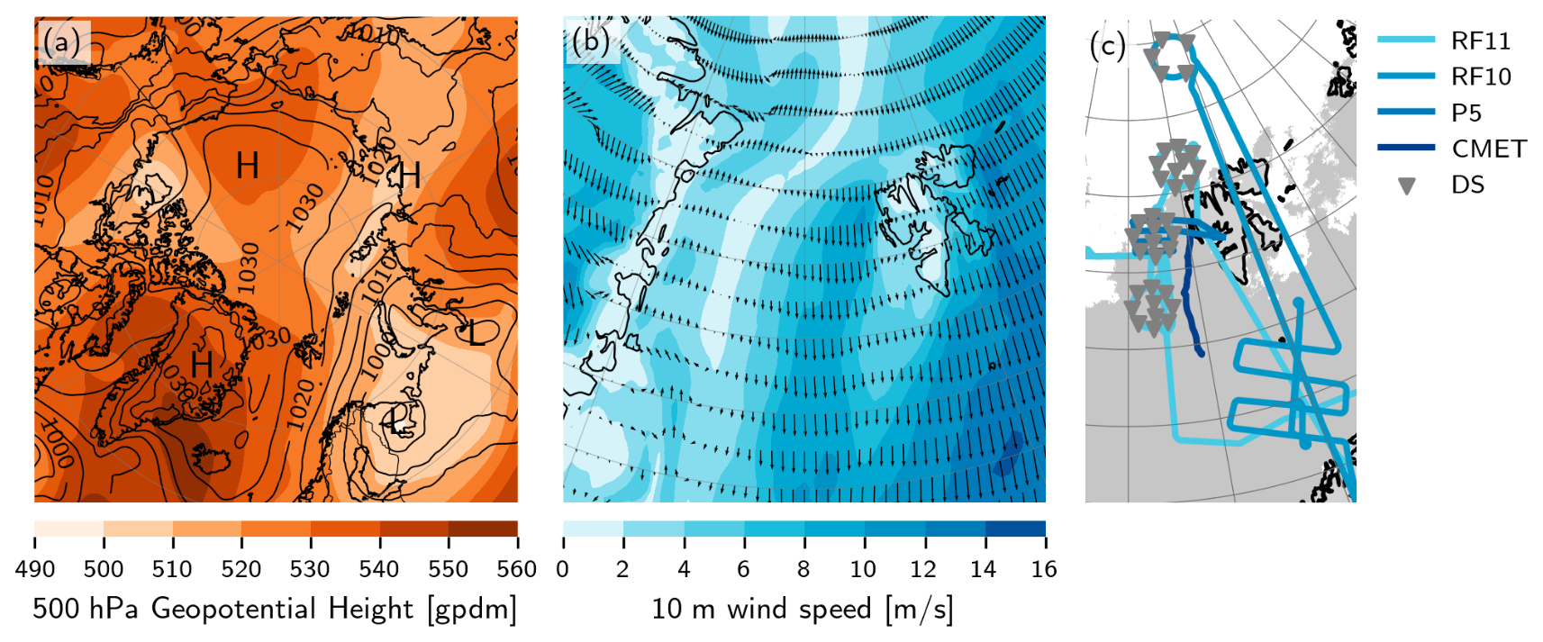
Figure A1 Maps of geopotential height at 500 hPa (shading) and mean sea level pressure (black contour lines; a) and wind speed at 10 m (shading) and wind direction (arrows) on 30 March 2022 at 12:00 UTC during HALO–(𝒜𝒞)³ from ERA5 (b). Flight paths of HALO flights RF10 (29 March 2022) and RF11 (30 March 2022) and P5 on 30 March 2022, together with CMET, Dropsonde (DS) locations (▾) and the sea-ice concentration retrieved from satellite observations (Spreen et al., 2008) indicated in grey and white (c).

Appendix B: Cold air outbreak and stability indices

Following Papritz and Spengler (2017) and Dahlke et al. (2022), the MCAO Index M is defined as the difference between the sea surface potential temperature ϑ_SKT and the potential temperature at 850 hPa ϑ_850 hPa:

$$\begin{array}{}\text{(B1)}& M={\mathit{\vartheta }}_{\text{SKT}}-{\mathit{\vartheta }}_{\text{850}\text{hPa}}\end{array}$$

Positive values indicate enhanced instability, favouring convection and cloud formation, while negative values point to a more stable boundary layer. Papritz and Spengler (2017) identify MCAO conditions if M>0 K and classify MCAOs as weak (0 K $<M\le \text{4}$ K), moderate (4 K $<M\le \text{8}$ K), strong (8 K $<M\le \text{12}$ K) and very strong (M>12 K). In Fig. B1 we present M as a function of latitude following the Lagrangian trajectory of the modelled air mass for the Ctrl simulation calculated from the model output, together with an estimation of M from the surface and dropsonde observations, using temperature and pressure profiles averaged over all sondes in one circle at the height level closest to 850 hPa for comparison.

The Stability Index is expressed as the ratio $\frac{z_i}{L}$, diagnosed from the model as the minimum local gradient of virtual potential temperature, and calculated from the averaged dropsonde profiles as the level that reaches a critical value of the bulk Richardson number Ri_b,crit>0.25 (ECMWF, 2016; Troen and Mahrt, 1986). The Obukhov length L characterises the role of buoyancy in turbulent flows:

$$\begin{array}{}\text{(B2)}& L=-{\displaystyle \frac{u_{*}^{\mathrm{3}}\stackrel{\mathrm{‾}}{{\mathit{\vartheta }}_{\mathrm{v}}}}{\mathit{\kappa }g(\stackrel{\mathrm{‾}}{w^{\prime }{\mathit{\vartheta }}_{\mathrm{v}}^{\prime }}{)}_{\mathrm{s}}}}\end{array}$$

with frictional velocity u_*, mean virtual potential temperature $\stackrel{\mathrm{‾}}{{\mathit{\vartheta }}_{\mathrm{v}}}$, surface virtual potential temperature flux $(\stackrel{\mathrm{‾}}{w^{\prime }{\mathit{\vartheta }}_{\mathrm{v}}^{\prime }}{)}_{\mathrm{s}}$ and Kármán constant κ (Stull, 1988). L is included in the model output and can be estimated from observations using a similar method by applying Monin–Obukhov similarity theory and iteratively solving the stability functions for L using Ri_b as an initial guess (Heus et al., 2010).

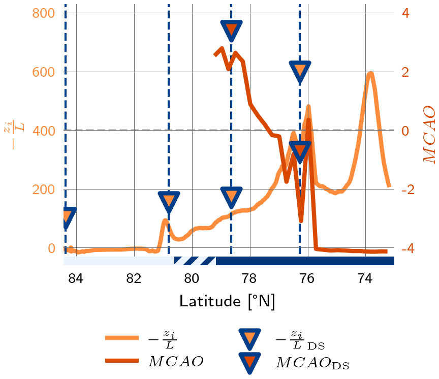
Figure B1 MCAO Index from Ctrl model output (red line) and from surface observations using VELOX and dropsonde profiles (red triangles). Stability index $-\frac{z_i}{L}$ from Ctrl model output (yellow line) and from observations (yellow triangles) along the simulation trajectory.

Appendix C: Trajectory calculation

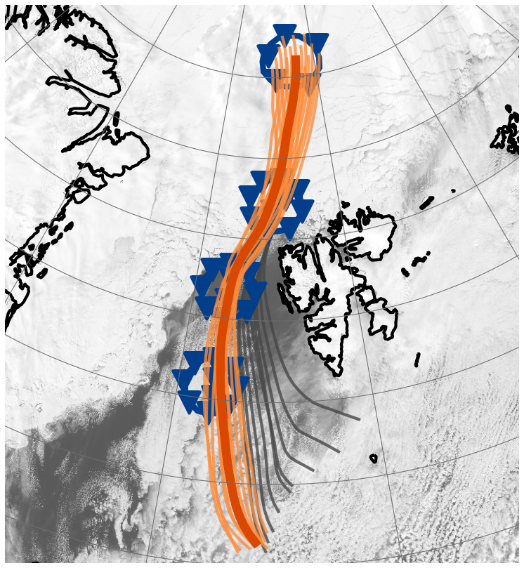
Figure C1 Lagrangian trajectories initiated inside IC at 870 hPa that were recaptured in C01, C02 and C03 (orange). Trajectories that were not resampled in the subsequent circle were discarded (grey) from the calculation of the mean trajectory used for the simulation (red). Dropsonde locations are marked with ▾. Satellite image at the time of RF11 29 March 2022 from Terra MODIS (NASA (2022), Worldview Snapshots) in the background.

Table C1 Summary of subsidence statistics derived from dropsonde observations for each circle. Mean values are computed over the full 8 km profile, while ranges and uncertainty estimates refer to the lowest 3 km.

Appendix D: Buoyancy flux evolution

The evolution of the Buoyancy Flux profile along the MCAO trajectory is shown in Fig. D1.

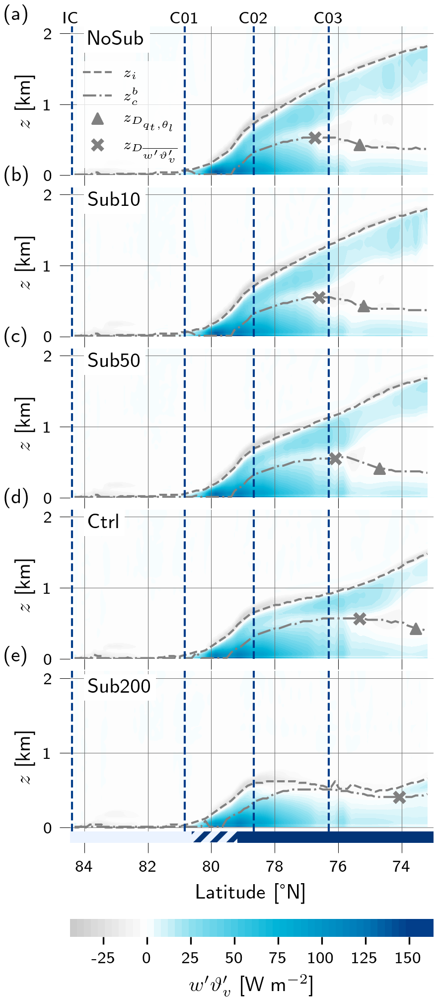
Figure D1 Latitudinal evolution of buoyancy flux along the MCAO trajectory for all sensitivity experiments. Dashed horizontal lines indicate dropsonde circle locations. Boundary layer height z_i and cloud base z_b are indicated by grey dashed and dot-dashed lines, respectively. The markers × and ▴ indicate decoupling points and heights with respect to w′ϑ_v′ and Δq_t and δϑ_l respectively. The coloured bar at the bottom indicates sea ice (sic >0.9, light blue), marginal sea-ice ($\text{0}<\mathrm{sic}\le \text{0.9}$, hatched), and open ocean (sic =0, dark blue).