Driving mechanisms for subsiding shells in simulations of deep moist convection

Downdrafts play an essential role in the feedback between convective clouds and their surrounding environment, and they must be properly accounted for in cumulus parameterizations (CPs). The mechanisms for downdraft formation are often debated in past literature and inconsistently represented in CPs. To address this uncertainty, we investigate the ring of descent surrounding cloudy updrafts known as a subsiding shell, a leading contributor to downdraft mass flux. We analyze two LES of deep convection in the Amazonian dry and wet season, using composite soundings from the Green Ocean Amazon Campaign. The dry and wet season soundings differ in their middle tropospheric relative humidity (RH), which facilitates an assessment of the influence of RH on shell strength. Kinetic energy budgets along trajectories reveal that shells acquire their descent from evaporatively driven negative effective buoyancy along cloud edge and downward oriented dynamic pressure accelerations associated with the toroidal circulations of updraft thermals. Consistent with observations, shell downdrafts were strongest in the dry season simulation. Contrary to hypotheses which attributed this difference to greater evaporative cooling, we find that dry season shell downdrafts associated with deep convection were stronger because of larger dynamic pressure accelerations in the dry season. However, when investigating cumulus congestus clouds, negative effective buoyancy accelerations become increasingly important relative to pressure accelerations. The stronger accelerations in deep convective shells were attributed to stronger dry season updrafts, and consequently more intense toroidal circulations within thermals. Our results provide a foundation of understanding for future improvement of downdraft representation in CPs.

1 Introduction

Since the turn of the century, global climate models (GCMs) have been used to further comprehend the future state of Earth's climate. However, with the consideration of computational expense, GCMs are run at coarse resolutions and cannot explicitly resolve important microscale and mesoscale features such as deep convection. Therefore, models rely heavily on parameterization schemes that account for sub-grid scale processes. One such scheme used in many climate models is a cumulus parameterization.

Cumulus parameterizations typically use a simplified model for updrafts and downdrafts to represent their sub-grid scale fluxes. The sub-grid scale vertical flux of water vapor can be organized into terms that consider both downdraft and updraft detrainment, as well as large scale subsidence (Bretherton and Smolarkiewicz, 1989). The detrainment of liquid water from a cloud into its environment is largely dependent on the vertical mass flux of updrafts associated with the clouds, and such detrainment allows for moistening of the ambient environment directly (Savre, 2021). Additionally, mass, momentum, and energy are transported downward via environmental subsidence away from convective clouds, which acts to warm and dry the surrounding environment. Parameterization schemes typically ensure that the sum of upward and downward fluxes equals the grid scale mass flux (Raymond, 1993). Though this handling of subsidence and downward mass transport appears both intuitive and practical, there are a few shortcomings. For instance, many parameterizations assume downdrafts displace mean grid state properties downward (Tiedtke, 1989; Bechtold et al., 2008; Park et al., 2016). However, downdrafts in the near-cloud environment may have substantially different properties than the mean grid state and may not follow the standard assumption of grid-wide redistribution of mass, heat, and momentum.

A near-cloud downdraft feature that has received research attention is the region of negative vertical velocity (w) immediately surrounding convective clouds. This subsidence area is commonly referred to as the subsiding shell and has been observed in the vicinity of shallow cumulus via aircraft observations (Jonas, 1990; Rodts et al., 2003; Katzwinkel et al., 2014; Mallaun et al., 2019). Subsiding shells are located at the cloud edge, protect cumulus clouds from dilution by allowing them to entrain pre-moistened air (Jonas, 1990; Rodts et al., 2003; Heus and Jonker, 2008; Dawe and Austin, 2011; Zhang et al., 2016; Hannah, 2017; Savre, 2021), and additionally serve as the primary contributor to downward heat and moisture transport above the boundary layer rather than convective compensating subsidence (Glenn and Krueger, 2014; Park et al., 2016).

There remains a debate concerning the mechanisms that drive downward accelerations in subsiding shells. Observational studies have found that shallow cumulus subsiding shells are primarily driven by negative thermal buoyancy B that arises from the evaporation of cloud droplets at cloud edge (Rodts et al., 2003; Siebert et al., 2006; Katzwinkel et al., 2014; Mallaun et al., 2019). In the presence of stronger cumulus updrafts, subsidence within the shell may further strengthen cloud edge turbulent mixing, increasing evaporative cooling and shell thickness in a positive feedback loop (Siebert et al., 2006; Nair et al., 2020). Estimates of entrainment in large eddy simulations (LESs) that assume clouds entrain unmodified air from the far field environment often underestimate the fractional entrainment rates of clouds (Romps, 2010; Dawe and Austin, 2011; Hannah, 2017) because these estimates neglect the moisture of shell air. Heus and Jonker (2008) confirmed via LES that evaporative cooling was the sole mechanism for shallow, non-precipitating cumulus subsiding shell formation and acceleration. Additionally, subsidence from downward B-driven accelerations was counteracted by upward vertical perturbation pressure gradient accelerations (VPG) within the shell (Heus and Jonker, 2008). Rodts et al. (2003) previously supplied evidence for this result with aircraft observations, noting that shells driven by pressure perturbations would contain a lower water vapor mixing ratio (q_v) than the surrounding environment since mass would be transported downward from cloud top, which is inconsistent with the aforementioned observational and modeling studies.

Additional mechanisms for subsiding shell formation have been explored as well. While finding some evidence for negative B as a driver in shell subsidence, Park et al. (2017) also noted that the spatial structure of shallow cumulus subsiding shells is consistent with the simple assumption that updraft thermals yield a vortex feature driven by horizontal B gradients whose outer branch drives the shell downward along cloud edge (Sherwood et al., 2013; Romps and Charn, 2015; Park et al., 2016). Jonas (1990) observed that shells encapsulating shallow maritime cumulus were formed via cloud-top pressure perturbations and the spherical vortex feature that arises from them, which is similar to Hill's vortex (Hill and Henrici, 1894), and were strengthened by evaporative cooling at cloud edge. Hence, it also appears possible that shells are sometimes driven by a VPG, and there is a lack of reconciliation between evaporation-driven and VPG-driven paradigms.

Generally, observational and LES studies focusing on shell formation from B reversal/evaporative cooling or toroidal circulations from cloud-top pressure perturbations have been confined to non-precipitating shallow cumulus clouds. However, aside from the work of Sherwood et al. (2013), Glenn and Krueger (2014), and Savre (2021), properties and formation mechanisms of subsiding shells surrounding tropical deep convective clouds are less commonly studied. Glenn and Krueger (2014) determined that compensatory downward mass flux associated with deep convection subsiding shells is 5 %–10 % of upward flux at any given level, highlighting their importance for mass transport. Such deep convective updrafts are susceptible to the effects of dynamic and turbulent entrainment (Morrison, 2016), which would yield strong evaporative cooling at cloud edge and shell formation. Additionally, thermal-like deep convective clouds with stronger updrafts generate cloud-top pressure perturbations that are greater in magnitude than that of shallow cumulus with significantly weaker updrafts (Parish and Leon, 2013; Morrison and Peters, 2018), increasing the potential importance of dynamic forcing of shells. Using LES, Savre (2021) determined that shells associated with deep moist convection were created by both mechanical, VPG-driven forcing near cloud top and by evaporative cooling away from cloud top. However, dynamic pressure forcing near cloud top appeared critical in Savre (2021) for explaining the magnitude of negative w in the shells. Given the variety of mechanisms driving shells in past literature, it is possible that the contributing mechanisms driving shell development in shallow cumulus and deep convection are environmentally dependent.

One natural laboratory for convection studies is the Amazon Rainforest in South America – a region where deep convection occurs relatively often (Giangrande et al., 2023). The Green Ocean Amazon (GOAMAZON) field campaign, performed in 2014 and 2015, supplied ample data for the analysis of deep convective clouds and their associated downdraft structures. Giangrande et al. (2023) determined that there were two distinct convective seasons that affected downdraft characteristics in the Amazon: a dry and wet season, both characterized by nearly identical temperature profiles but varying in free tropospheric relative humidity (RH) (Giangrande et al., 2020, 2023). Such RH variation could have significant impacts on convective behavior, especially in relation to mixing of cloudy and environmental air (Derbyshire et al., 2004). The dry season, which persists from June through September, is characterized by larger most-unstable convective available potential energy (MUCAPE), while the wet season (December–April) has reduced MUCAPE and marginally less vertical wind shear (Giangrande et al., 2020, 2023). Vertically oriented radar wind profilers observed a higher incidence of strong downdrafts in the dry season than in the wet season. There are a variety of potential explanations for this difference. One hypothesis offered in their study was:

downdrafts occurring in the vicinity of updrafts are stronger in the dry season because the drier air in the free troposphere in the dry season led to greater evaporative cooling along cloud edge (Giangrande et al., 2023).

This hypothesis implies a dominant role of B in modulating downdraft strength, and that environmental variations in downdraft strength are primarily modulated by thermodynamic differences aloft, such as whether the free troposphere is moist or dry. However, Giangrande et al. (2023) also found some differences in updraft behavior including stronger updrafts at low-levels in the dry season. Hence, an equally plausible hypothesis is:

differences in updraft strength contributed to commensurate differences in downdraft strength via the downward-oriented VPG within rising cloud thermals.

We intend to leverage these environmental, updraft, and downdraft observations sampled in GOAMAZON to address the aforementioned hypotheses, providing reconciliation of past ambiguity about the mechanisms that drive subsiding shells in deep convection. Two LESs and a Lagrangian parcel trajectory analysis are used to further assess the accelerations driving shell formation and maintenance. The next section provides a description of the LES setup and trajectory analysis used for shell investigation. Results of shell properties, the role of environmental RH in shell formation, and the comparison between deep and congestus shells will follow. Conclusions from this work and future research will be established in the final section.

2 Methodology

Two idealized LESs of deep moist convection were run using Cloud Model 1 version 21.0 (CM1; Bryan and Fritsch, 2002). Both LES were run with an isotropic 100 m grid spacing over a 200 km² domain, with a depth of 20 km. While the selected horizontal grid spacing is coarse relative to other subsiding shell modeling studies (e.g., 50 m in Heus and Jonker, 2008 and 25 m in Park et al., 2017), computational expense limits us from utilizing a finer grid spacing. Additionally, the previously-mentioned modeling studies focus on shallow cumulus, where the narrowest subsiding shells are 100–200 m wide. Savre (2021) found that shells associated with deep convection were 800 m wide, on average, with maximum widths of upwards of 2000 m. With this, we believe our 100 m horizontal grid spacing is sufficient in resolving deep convective subsiding shells. To ensure this, we performed grid spacing sensitivity simulations, which are discussed in Appendix A.

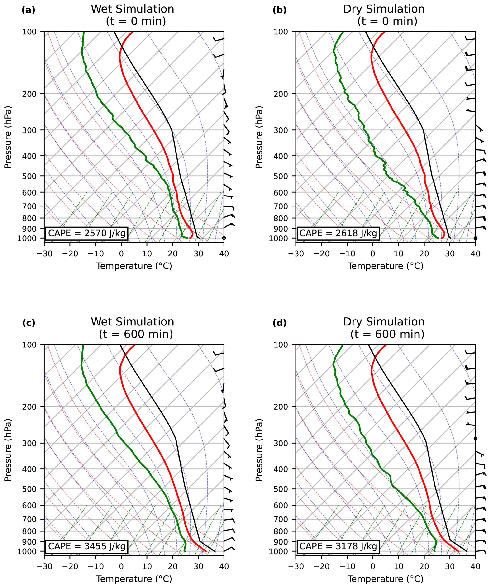
Figure 1 Skew-T Log-P diagrams of initial GOAMAZON (a) wet and (b) dry season composited soundings used for LESs. Panels (c) and (d) are simulated soundings 10 h into the simulation for the wet and dry season, respectively. The red and green lines are environmental temperature and dewpoint temperature, respectively. Black curves represent the density temperature of an undiluted lifted surface parcel. Wind barbs are in units of knots and are plotted on the right side of each panel. Surface-based CAPE is listed in the legends, calculated using the adiabatic lapse rate formulas from Peters et al. (2022b) and Peters (2024).

The simulations differed from each other only with respect to their input atmospheric profiles. One simulation was initialized with the GOAMAZON wet season composite sounding (referred to the “wet simulation”). Similarly, the second simulation was run using the dry season profile (referred to as the “dry simulation”). Each sounding included in the composited sounding was taken at 12:00 UTC before a convective event. Though both seasons have similar temperature profiles, we set them equal to each other (both having that of the dry season; Fig. 1a, b) for simplicity to isolate the influences of RH on downdrafts (Fig. 2). The moisture profile of the boundary layer in both simulations is similar, but the RH spread between the two simulations increases above 2 km. In much of the free troposphere, the wet simulation RH magnitudes are 20 %–40 % greater than the dry simulation at any given height. RH magnitudes become comparable above 11 km, but most deep convective clouds that are investigated in this study do not reach this height. The wind profiles of the simulations also differ with slightly stronger vertical wind shear present in the dry season than in the wet season. Though simulation wind profiles differ, wind shear is weak and differences in convective characteristics attributed to wind shear are likely small.

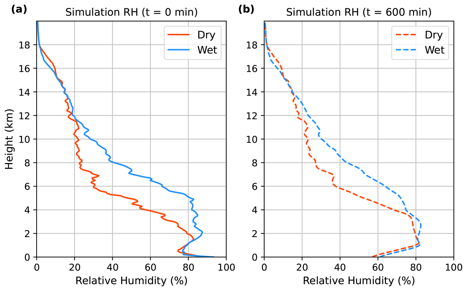
Figure 2 (a) Initial and (b) hour 10 profiles of environmental RH (%, x-axis) as a function of height (km, y-axis) for the dry (red) and wet (blue) simulation.

Sub-grid scale turbulence was parameterized using the turbulent kinetic energy scheme (e.g., Deardorff, 1980) and Morrison double-moment microphysics (Morrison et al., 2005, 2009) were used in both simulations. The Morrison double-moment scheme was used because it predicts both mixing ratio and number concentration for species crucial to our shell identification, including cloud water and cloud ice which are used to identify cloud edge. In our simulations, the scheme allows for resolved supersaturation and droplet activation is determined via Kohler theory rather than a reliance on the subgrid w (Morrison et al., 2005). Lateral boundary conditions were periodic and both vertical boundaries were free slip. Simulations were spun-up with random potential temperature perturbations of ±0.25 K sampled from a uniform distribution, along with a constant surface potential temperature flux of 0.06 K m s⁻¹ (a typical late morning value for Amazon heat flux; e.g., Malhi et al., 2002; da Rocha et al., 2004), and a constant water vapor mixing ratio (q_v) flux of 2 × 10⁻⁴ kg kg⁻¹ m s⁻¹ (chosen via trial-and-error to prevent over-drying of the boundary layer). All other model settings were left at their default values available in the CM1 version 21.0 source code.

Because detrainment from simulated convection led to large scale moistening of the ambient environment, nudging of the domain-averaged q_v toward the initial moisture profile for each simulation was applied above 4 km with a time scale of 6 h over the course of the simulation to isolate the RH impacts on convection. This method of relaxation nudging is described in Alland et al. (2021), where the domain-averaged profile is relaxed towards its initial state over a specified time scale. This allowed for the environments in the simulations to retain their distinctly different initial free-tropospheric moisture profiles (Fig. 2a), characteristic of differences between the wet and dry seasons. RH profiles after a 10 h spin-up period are shown in Fig. 2b. Nudging was only applied above 4 km to allow for surface fluxes to grow a well-mixed boundary layer unimpeded. Although the layer between the boundary layer and 4 km was not nudged and could freely evolve, comparison of the initial and 10 h RH profiles shown in Fig. 2 reveals that RH in this layer was only slightly altered. However, the atmosphere continues to evolve over large time scales, so longer analysis periods may experience greater differences from start to end.

Maximum w became steady in both simulations by 10 h, suggesting that the cloud population in both simulations had achieved an approximate steady state. As mentioned in the previous paragraph, the layer between the boundary layer top and 4 km was not nudged and could freely evolve. Therefore, the convection in our simulations is not truly in a steady state. However, with maximum w becoming steady, we can assume that the characteristics of the convection undergo limited changes despite the slight RH variation in the lower troposphere. At 10 h, model output frequency increased to 30 s for the following hour. This allowed for direct comparison between parcel properties and model properties without the need for temporal interpolation. Additionally, all analysis of subsiding shell properties was performed during this hour.

Subsiding shells were identified following the methodology of Savre (2021) by first defining clouds as regions with total condensate (q_c+q_i) greater than 0.01 g kg⁻¹, where q_c and q_i are cloud water and ice mixing ratios, respectively. Cloud edge was then defined where cloudy points were immediately adjacent to non-cloudy points. Following cloud edge identification, an algorithm was applied to step outward from cloud edge and add all continuous grid points in the horizontal and vertical where w<0 m s⁻¹. There was no B criterion included in the search to avoid making an a-priori assumption that subsiding shell downdrafts are solely driven by negative B.

Parcel trajectories were tracked through subsiding shells using the built-in Lagrangian parcel trajectory analysis included in the CM1 software package. At the initial time step, 5,494,536 parcels were distributed uniformly every 100 m from 1.5 to 15 km in the vertical and every 500 m horizontally across the entire domain. Parcel location, w, B, and VPG accelerations were output every 30 s for each parcel during the analysis period. Previous Lagrangian parcel studies have output parcel properties every few seconds to minutes (e.g., Hernandez-Deckers and Sherwood, 2016), but given that parcels are often within shells on the order of minutes, the 30 s parcel output is sufficient in assessing shell parcel properties while considering computational expense.

Buoyancy in CM1 is computed via the following formula:

$$\begin{array}{}\text{(1)}& B=g\left({\displaystyle \frac{\mathit{\theta }-{\mathit{\theta }}_{\mathrm{0}}}{{\mathit{\theta }}_{\mathrm{0}}}}\right)+g\left({\displaystyle \frac{R_{\mathrm{v}}}{R_{\mathrm{d}}}}-\mathrm{1}\right)\left(q_{\mathrm{v}}-q_{\mathrm{v},\mathrm{0}}\right)-g{q}_{\mathrm{con}},\end{array}$$

where g is the gravitational constant, θ is potential temperature, R_v and R_d are the specific gas constants for water vapor and dry air respectively, q_con is the total condensate mixing ratio, and 0 subscripts denote the height-only dependent initial model profile (i.e., the soundings represented in Fig. 1a, b). Because of the hydrostatic responses to the input of surface fluxes and adjustments of the large-scale atmosphere to convection, horizontal mean layers of the model domain attain large positive and negative B after several hours of simulation. These layers are hydrostatically balanced, and do not contribute meaningfully to the accelerations occurring within subsiding shells. To make for cleaner physical interpretation of the distinct physical processes contributing to B accelerations, the horizontal mean of B on a given level at each time was subtracted from the value of B on that level at a given grid point, and added to the VPG at that grid point. This adjustment removes the horizontally-averaged hydrostatically balanced B, isolating the local B relevant to convective processes.

Downdraft parcels that passed through subsiding shells were analyzed. Initially, downdraft parcels were defined as those that met three criteria. Parcels must (a) begin their downdraft at a height of 5 km or greater, (b) reach a minimum w of −1.5 m s⁻¹ or stronger, and (c) undergo a permanent vertical displacement of at least 500 m in one downdraft swath. The height and w criterion were implemented to ensure parcels were associated with deep convective downdrafts and not within a large-scale subsidence or gravity wave regime. Following this filtering, only parcels that passed through subsiding shell points for 90 % of their downdraft life (period where w<0) were analyzed.

The prognostic pressure variable in CM1 is $\mathit{\pi }={\left(\frac{p}{p_{\mathrm{ref}}}\right)}^{\frac{R_{\mathrm{d}}}{c_p}}$, where p is pressure, p_ref=1000 hPa is a reference pressure, R_d is the specific gas constant for dry air, and c_p is the specific heat capacity at constant pressure. Pressure in our simulations is explicitly solved for using compressible equations with Klemp-Wilhelmson time-splitting (psolver = 2 in the CM1 namelist file), which is recommended when horizontal and vertical grid spacings are nearly equal (Bryan and Fritsch, 2002). To attribute vertical pressure accelerations to distinct physical processes, we decompose π into buoyant (${\mathit{\pi }}_B^{\prime }$) and dynamic (${\mathit{\pi }}_D^{\prime }$) contributions. These contributions are obtained from the following equations (e.g., Klemp and Rotunno, 1983):

$$\begin{array}{}\text{(2)}& {\displaystyle }\mathrm{\nabla }\cdot \left(c_p{\mathit{\theta }}_{\mathrm{0},\mathit{\rho }}\mathrm{\nabla }{\mathit{\pi }}_B^{\prime }\right)={\displaystyle \frac{\partial \left({\mathit{\rho }}_{\mathrm{0}}B\right)}{\partial z}},\text{(3)}& {\displaystyle }\mathrm{\nabla }\cdot \left(c_p{\mathit{\theta }}_{\mathrm{0},\mathit{\rho }}\mathrm{\nabla }{\mathit{\pi }}_D^{\prime }\right)=-\mathrm{\nabla }\cdot ({\mathit{\rho }}_{\mathrm{0}}\mathit{V}\cdot \mathrm{\nabla }\mathit{V}),\end{array}$$

where θ_0,ρ and ρ₀ are the initial height-dependent density potential temperature and density, respectively, and V is the three-dimensional wind vector.

Further decomposition of ${\mathit{\pi }}_D^{\prime }$ and the right-hand side of the above equation into linear (${\mathit{\pi }}_{\mathrm{DL}}^{\prime }$) and nonlinear (${\mathit{\pi }}_{\mathrm{DN}}^{\prime }$) terms gives:

$$\begin{array}{}\text{(4)}& {\displaystyle }\mathrm{\nabla }\cdot \left(c_p{\mathit{\theta }}_{\mathrm{0},\mathit{\rho }}\mathrm{\nabla }{\mathit{\pi }}_{\mathrm{DN}}^{\prime }\right)=-\mathrm{\nabla }\cdot ({\mathit{\rho }}_{\mathrm{0}}{\mathit{V}}^{\prime }\cdot \mathrm{\nabla }{\mathit{V}}^{\prime }),\text{(5)}& {\displaystyle }\mathrm{\nabla }\cdot \left(c_p{\mathit{\theta }}_{\mathrm{0},\mathit{\rho }}\mathrm{\nabla }{\mathit{\pi }}_{\mathrm{DL}}^{\prime }\right)=-{\mathit{\rho }}_{\mathrm{0}}\mathrm{\nabla }w\cdot {\displaystyle \frac{d{\mathit{V}}_{\mathrm{0}}}{\mathrm{d}z}},\end{array}$$

where V₀ is the simulation's initial horizontal wind profile and ${\mathit{V}}^{\prime }\equiv \mathit{V}-{\mathit{V}}_{\mathrm{0}}$. The direct calculation of ${\mathit{\pi }}_B^{\prime }$ and ${\mathit{\pi }}_{\mathrm{DL}}^{\prime }$ was completed by using a Fourier transform method in the horizontal and a tri-diagonal solver in the vertical, following the method used in CM1 (Bryan and Fritsch, 2002). ${\mathit{\pi }}_{\mathrm{DN}}^{\prime }$ was then calculated as a residual. Retrieval of VPG accelerations via centered finite differences was completed following this decomposition. The decomposed VPG accelerations that arise from the computation of perturbation pressure were mapped onto shell parcel trajectory locations using trilinear interpolation.

Physically, ${\mathit{\pi }}_{\mathrm{DN}}^{\prime }$ is dependent on the local vorticity and deformation magnitudes. It is regions of relative low ${\mathit{\pi }}_{\mathrm{DN}}^{\prime }$ that are associated with the toroidal circulation in thermal convection, and hence dynamically forced accelerations will show up in the component of the VPG driven by ${\mathit{\pi }}_{\mathrm{DN}}^{\prime }$. The linear dynamic pressure ${\mathit{\pi }}_{\mathrm{DL}}^{\prime }$ relates to the interaction of the updraft with the background environment shear profile. As we will see, the component of VPG from ${\mathit{\pi }}_{\mathrm{DL}}^{\prime }$ is typically small relative to ${\mathit{\pi }}_{\mathrm{DN}}^{\prime }$ and ${\mathit{\pi }}_B^{\prime }$ due to the relatively weak vertical shear in both the wet and dry season environments. ${\mathit{\pi }}_B^{\prime }$ is inversely related to vertical gradients in B itself, with high ${\mathit{\pi }}_B^{\prime }$ occurring where B decreases most rapidly with height. Hence, the VPG from ${\mathit{\pi }}_B^{\prime }$ is connected to B within the updraft and subsiding shell regions, which are distinctly separate processes from the dynamical accelerations driven by the toroidal circulations.

Because a large spectrum of cloud depths can be lumped into a “deep” convective regime, shell parcels and the shells themselves were investigated in two subgroups: a deep regime and a congestus regime. This was done to focus on mature and deepening convection, while removing shallow cumulus from the analysis. We defined congestus based on the criteria found in Jensen and Genio (2006), with congestus clouds having cloud top heights below 5 km and deep cloud tops exceeding 5 km. Deep and congestus parcels were gathered by taking previously defined shell parcels and placing them into their respective group based on origin height.

To connect parcel accelerations to cloud features, vertical composites of shells and their parent updrafts were created for the hour of analysis. First, we identified cloudy updrafts as continuous regions of w>0 m s⁻¹ and $q_{\mathrm{c}}+q_{\mathrm{i}}>\mathrm{1}\times {\mathrm{10}}^{-\mathrm{5}}$ kg kg⁻¹, with a maximum w>3 m s⁻¹ and a depth of at least 1 km. We then found the centroid of this feature by averaging the position of all grid points. A 3D box was then placed around the cloud with a horizontal width of 6 km and a height of 8 km. The shell minimum was then identified as the minimum w in the box within 800 m of the shell point closest to the updraft. The 800 m horizontal threshold was chosen in conjunction with findings from Savre (2021), where it was determined that subsiding shells associated with deep convection were 800 m wide, on average. This threshold was also chosen to avoid sampling shells from surrounding clouds or other features away from the updraft of interest. Deep convective shells in the Savre (2021) were found to be upwards of 2000 m wide, despite a conservative deep convection depth threshold of 1500 m. As will be shown, the convection in the present study's simulations exceeds this depth and, with wider shells being associated with deeper convection, the maximum shell edge to shell core distance of 800 m is appropriate. We then composited fields within a vertically integrated plane that intersected the shell minimum w and updraft centroid. Lastly, all vectors from updraft maximum w to shell minimum w were rotated to be aligned on a common axis and all fields were normalized by fractional distance from updraft maximum w to shell minimum w. B, B_eff, and VPG accelerations were composited in the same way, as well as q_v, ${\mathit{\pi }}_B^{\prime }$, and ${\mathit{\pi }}_{\mathrm{DN}}^{\prime }$.

3 Results

3.1 Differences in Updraft Properties

A well-mixed layer formed adjacent to the lower boundary in both simulations and gradually deepened through the 10 hours preceding our analysis window (not shown). Deepening of the boundary layer allowed for the widespread development of slow-moving convection by the start of the analysis period. Cloud and updraft depths in both simulations gradually deepened during the 10 h spin-up time period, eventually reaching quasi-steady heights in the 14–16 km range (Fig. 3). Updraft top heights peaked in the 12–16 km range in both simulations, which is broadly consistent with echo top heights observed from GOAMAZON (e.g., Fig. 1a, b in Giangrande et al., 2023). Also consistent with the updraft observations analyzed in Giangrande et al. (2023) (their Fig. 5a–c), time-averaged maximum w was greater in the dry season simulation (∼ 31 m s⁻¹) than in the wet season simulation (∼ 27 m s⁻¹), and peak updraft intensities occurred lower in the atmosphere in the dry simulation than in the wet season simulation (Fig. 3c), though updrafts above roughly 10 km were stronger in the wet season simulation.

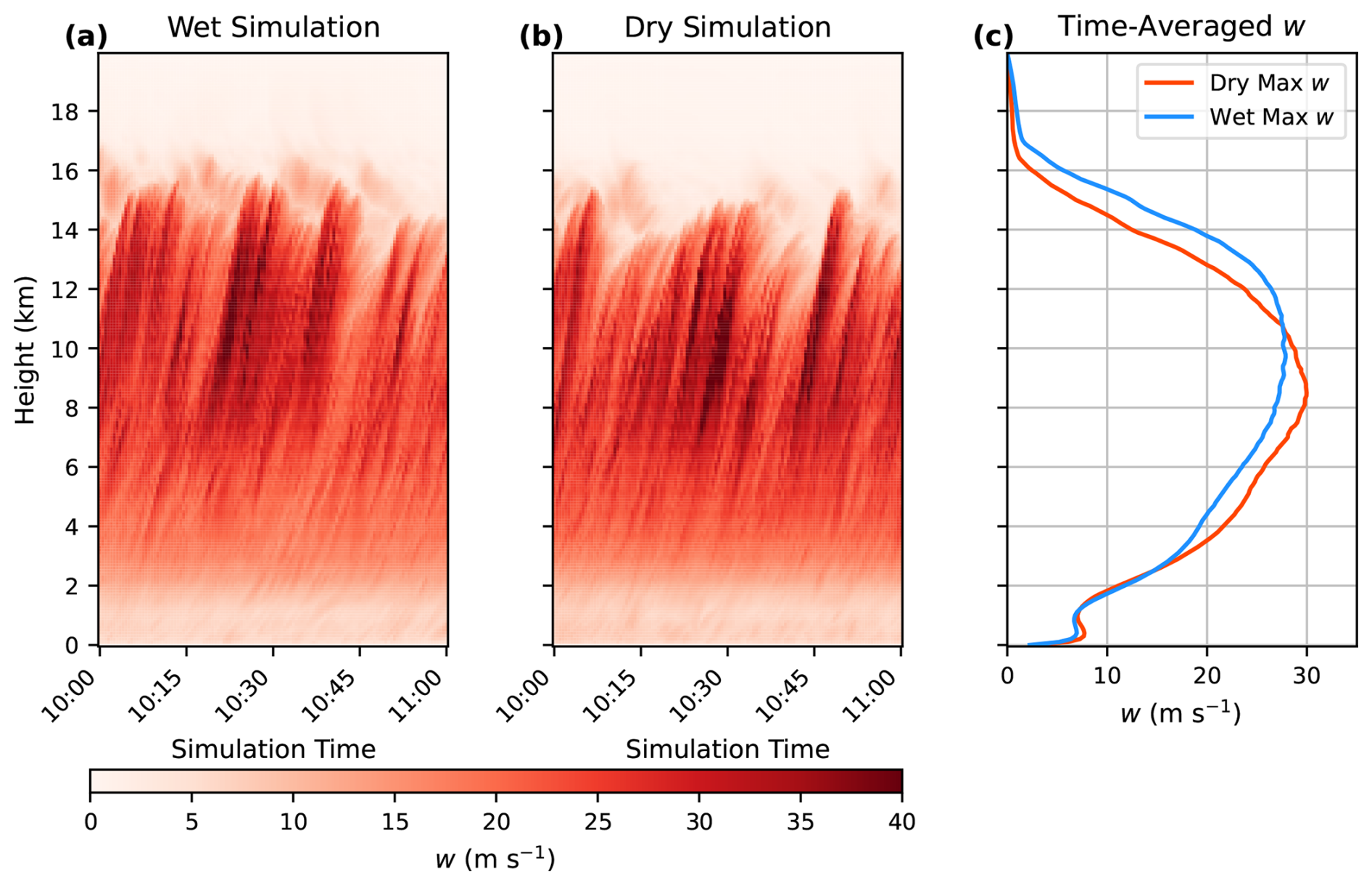
Figure 3 Vertical Hovmöller diagrams of horizontal domain maximum w with height during the period of analysis for the (a) wet simulation and (b) dry simulation. Vertical profile of time-averaged w during the analysis period for both simulations is exhibited in panel (c).

In addition to deep convection, congestus convection developed as well. Cloud properties of convection in the deep and congestus regime differ which, as shown in Sect. 3.3, has large implications on the behavior of accelerations driving subsiding shells. Deep convection is wider than that of congestus and is often characterized by multiple updraft thermals. The strongest surface-reaching downdrafts and heaviest precipitation are also associated with simulated deep convection. Though significant heterogeneity exists among cloud structures within each regime, examples of cloud structures in the deep and congestus regimes are shown in Fig. 4. Subsiding shells are present at cloud edge near cloud top in both the deep and congestus clouds in Fig. 4, as well as down the entire right side of the congestus cloud.

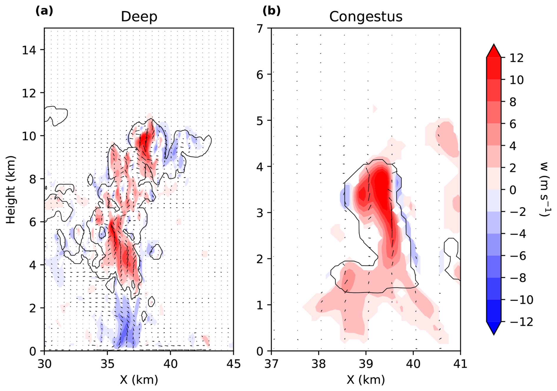
Figure 4 Vertical cross sections of w for a cloud in the (a) deep and (b) congestus regime. Regions with $\left|w\right|<\mathrm{1}$ m s⁻¹ are masked out. Cloud edge is outlined with a black contour. The local flow field with the horizontally-averaged wind removed is depicted with quivers.

As will be shown later, differences in updraft intensity and vertical distribution between the dry and wet season simulations were important contributors to commensurate differences in shell intensities. We demonstrate the physical reasons for these differences by examining the temperature and moisture, the B of lifted surface parcels in the 10 h sounding, and by applying a simple updraft model. In this model, a surface parcel is lifted and diluted with a fractional entrainment rate ε calculated from the following formula:

$$\begin{array}{}\text{(6)}& \mathit{\epsilon }\equiv {\displaystyle \frac{\mathrm{2}{k}^{\mathrm{2}}L}{P_r{R}^{\mathrm{2}}}},\end{array}$$

where k²=0.18 is the squared Von-Karman constant, $P_r=\frac{\mathrm{1}}{\mathrm{3}}$ is the turbulent Prandtl number, L=200 m is a mixing length, and R is the updraft radius. This formula was derived in Morrison (2017) based on an eddy diffusivity approximation for lateral mixing. We set R to the lifting condensation level (LCL) height for a surface parcel calculated using the formula from Romps (2017), consistent with past studies that have shown correlations between the LCL height and updraft radius (Mulholland et al., 2021). The thermodynamic properties and B of the surface parcel were calculated using methods described in Peters et al. (2022b) and Peters (2024), which include hydrometeor loading and ice processes. Using this B profile, w was calculated using the updraft plume model from Peters et al. (2022a) (see their Appendix A).

Vertical profiles of $\mathrm{\Delta }{T}_{\mathrm{0}}\equiv T_{\mathrm{0},\mathrm{wet}}-T_{\mathrm{0},\mathrm{dry}}$ (Fig. 5a), where the T₀ variables are the horizontal averages of T shown in Fig. 1c, d, reveal warmer temperatures (i.e., positive ΔT₀) at low-levels in the wet simulation than in the dry simulation at 10 h, particularly in the 2–7 km layer. This difference resulted in smaller undiluted adiabatic B in the 2–7 km layer in the wet simulation (blue dashed lines in Fig. 5b) than in the dry simulation (red dashed lines in Fig. 5b), which also translated to a commensurate difference in diluted B (solid lines in Fig. 5b). Using the profiles of diluted B, the updraft model (Fig. 5c) yields profiles of wet season (solid blue) and dry season (solid red) w that closely mimic the time averaged profiles from the simulations (see Fig. 3c). The larger low-level diluted B in the dry simulation partially explains the stronger low-level updraft strengths in the dry simulation than in the wet simulation.

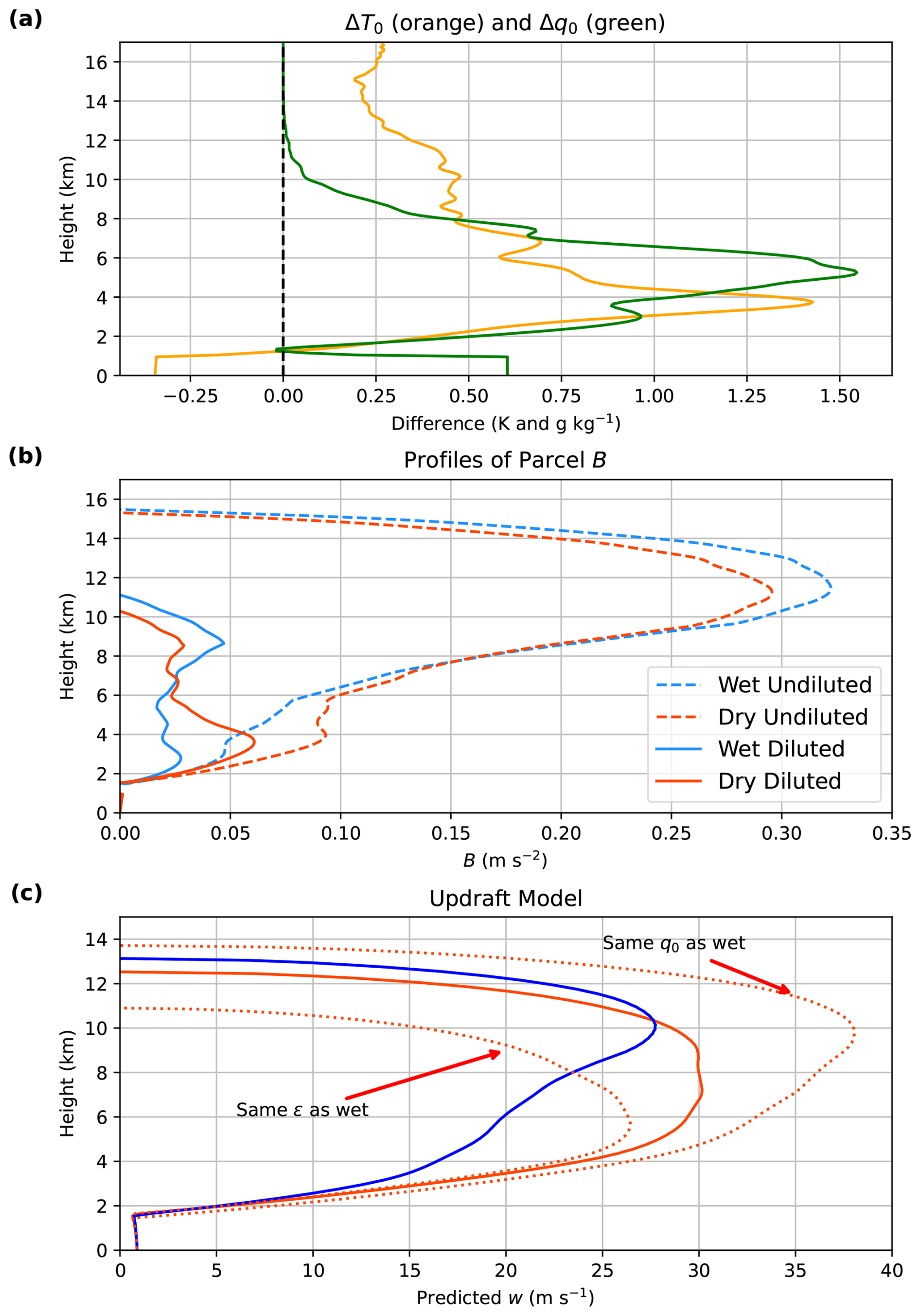
Figure 5 Profiles of (a) ΔT₀ (orange, K) and Δq₀ (green, g kg⁻¹) at 10 h (Δ indicates wet season minus dry season), (b) undiluted B (dashed lines) and diluted B (solid lines) for parcels lifted from the surface using the 10 h horizontal mean wet season (blue) and dry season (red) profiles, and (c) plume model w (m s⁻¹) predicted from the 10 h horizontal mean profiles (solid lines) for the wet season (blue) and dry season (red) simulations. Dashed red lines depict plume model w with the ε from the wet season applied to the dry season parcels (left dashed line) and the q₀ profile from the wet season applied to the dry season profile (right dashed line).

The differences in moisture between the wet and dry simulation also influenced the differences in w among the simulations. For instance, vertical profiles of $\mathrm{\Delta }{q}_{\mathrm{0}}\equiv q_{\mathrm{0},\mathrm{wet}}-q_{\mathrm{0},\mathrm{dry}}$ reveal smaller surface and lower tropospheric moisture (green line is positive in Fig. 5a) in the dry simulation. Because of this, the dry simulation developed a higher LCL height (1285 m) than the wet simulation (1166 m), which contributed to wider updrafts and smaller ε in the dry simulation, resulting in strengthened updrafts relative to the wet simulation. We deduce this because neglecting this difference in ε in the updraft model (left-most dotted red line in Fig. 5c) results in weaker maximum w in the dry profile than in the wet profile, which is inconsistent with the simulations. On the other hand, a drier lower free troposphere enhanced dilution in the dry simulation relative to the wet, which moderated w in the dry simulation and resulted in stronger updrafts aloft in the wet simulation. We deduce this because replacing the moisture profile in the dry profile with that of the wet and re-running the updraft model results in a dry season w that is erroneously stronger than the wet season w at all levels (right-most dotted red line in Fig. 5c).

3.2 Driving Mechanisms for Subsiding Shells

Utilizing parcel trajectories, subsiding shell properties were assessed in bulk. Dry and wet simulation shell parcel w are displayed in Fig. 6. The normalized downdraft time coordinate in Fig. 6a allows parcel properties to be compared based on downdraft start time and downdraft end time, whereas the normalized height coordinate in Fig. 6b is used to compare parcel properties based on downdraft origin height and termination height. Immediately, it is evident that use of the normalized height coordinate yields stronger shells. This is because the strongest shell subsidence may occur at different times in the downdraft but always occurs about halfway down the downdraft. For the remainder of this analysis, we choose to use the normalized time coordinate (Fig. 6a) because understanding time evolution of parcel properties such as acceleration is prioritized in this study. To avoid performing a temporal interpolation of trajectories, the first downdraft point for each parcel is the first time step in which w<0 m s⁻¹. As a result, trajectory w does not begin at 0 m s⁻¹, but rather at some value below it. Immediately, it is evident that dry shell downdrafts are stronger than those in the wet simulation, consistent with the RWP observations in Giangrande et al. (2023). Mean wet simulation shell parcel w reached a mean minimum of −2.78 m s⁻¹, whereas dry shell parcels achieved a mean minimum w of −3.44 m s⁻¹. This equates to dry simulation downdrafts being 23.5 % stronger than their wet simulation counterparts. Statistical significance in the difference of the means was determined using a Welch's t-test with a significance level (α) of 0.05. Mean differences were statistically significant through the entire downdraft period, with dry simulation downdrafts on average being 26.5 % stronger than those in the wet simulation.

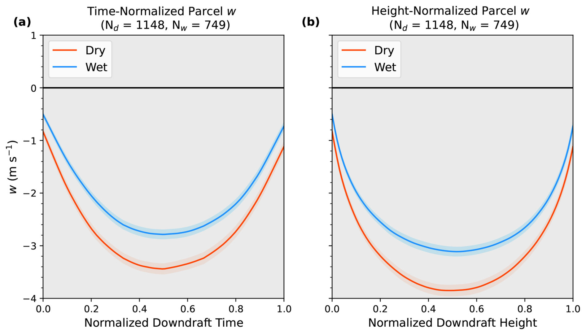
Figure 6 Mean subsiding shell parcel w through (a) normalized downdraft time and (b) normalized height for the dry (red) and wet (blue) simulations. 95 % confidence intervals are shaded for each simulation and parcel sample size is noted above each panel. Grey shading indicates areas where simulation differences are statistically significant with α = 0.05. N_d and N_w denote the sample size of dry and wet simulation parcels, respectively.

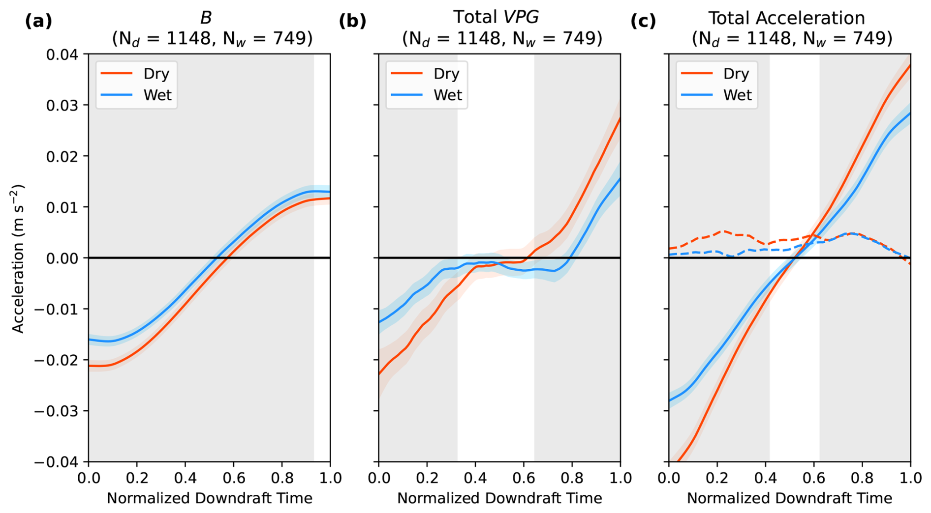
Figure 7 Mean subsiding shell parcel (a) B, (b) VPG, and (c) total acceleration through normalized downdraft time for the dry (red) and wet (blue) simulations. Acceleration from subgrid processes for the dry and wet simulations is depicted in panel (c) with red and blue dashed lines, respectively. 95 % confidence intervals are shaded for each simulation and parcel sample size is noted above each panel. Grey shading indicates areas where simulation mean differences are statistically significant with α=0.05.

Mean accelerations acting on subsiding shell parcels are shown in Fig. 7. With regard to total accelerations, it is evident in both simulations that parcels that pass through shells are both negatively buoyant and are initially accelerated downward by VPG accelerations. Though not shown, parcels experienced minima in downward accelerations from both total VPG and B a few seconds to minutes before achieving a negative w. In Fig. 7a, subsiding shell parcels in the dry simulation are initially more negatively buoyant with a minimum average B of −0.021 m s⁻². B then increases through ≈ 55 % of the downdraft time, at which point B sign reversal occurs and B becomes positive due to parcels overshooting their level of neutral B. Wet simulation mean B, which is most negative at shell downdraft initialization with a value of −0.016 m s⁻², shares a similar increasing trend to that of the dry simulation. Like B, the VPG (Fig. 7b) is initially negative and decreases in magnitude as parcels descend. With an initial VPG of −0.023 m s⁻², dry simulation VPG acceleration becomes positive ≈ 60 % of the way through the downdraft before reaching a maximum of 0.027 m s⁻² at downdraft end. However, unlike B which increases continuously, dry simulation VPG accelerations plateau halfway through the downdraft. The wet simulation VPG undergoes the same behavior, albeit with both smaller downward accelerations initially, and smaller upward accelerations later on. Statistical significance of B and VPG acceleration behaviors was assessed as well. B differences were significant through the entirety of the downdraft, while VPG differences showed significance through the first and final ≈ 35 % of the downdraft. With this, differences in total acceleration means are significant in both the cloud-top region where the shells initiate and the shell terminus.

One acceleration that must also be addressed is that from subgrid scale processes such as turbulence. The subgrid scale acceleration, which does contribute to total acceleration within shells, is plotted in Fig. 7c. Though the acceleration is weak compared to B and VPG, it ultimately provides a dampening effect in both the dry and wet simulations. This subgrid term is likely physically representative of turbulent mixing. Because we see dampening, it is likely that, while shells are accelerated downward by B and VPG, turbulent mixing of updraft or environmental air into the shell acts to reduce net downward acceleration. This upward acceleration persists through the entirety of the downdraft. As for seasonal differences, dry season subgrid effects are larger than that of the wet season. Because turbulent mixing is tied to the horizontal shear at the interface of the updraft and shell, and since dry simulation updrafts and shells are stronger, the dampening effect from dry simulation turbulent mixing is greater as well.

Figure 8 Same as Fig. 7, but for (a) VPG_DN, (b) VPG_B, (c) B_eff, and (d) VPG_DL.

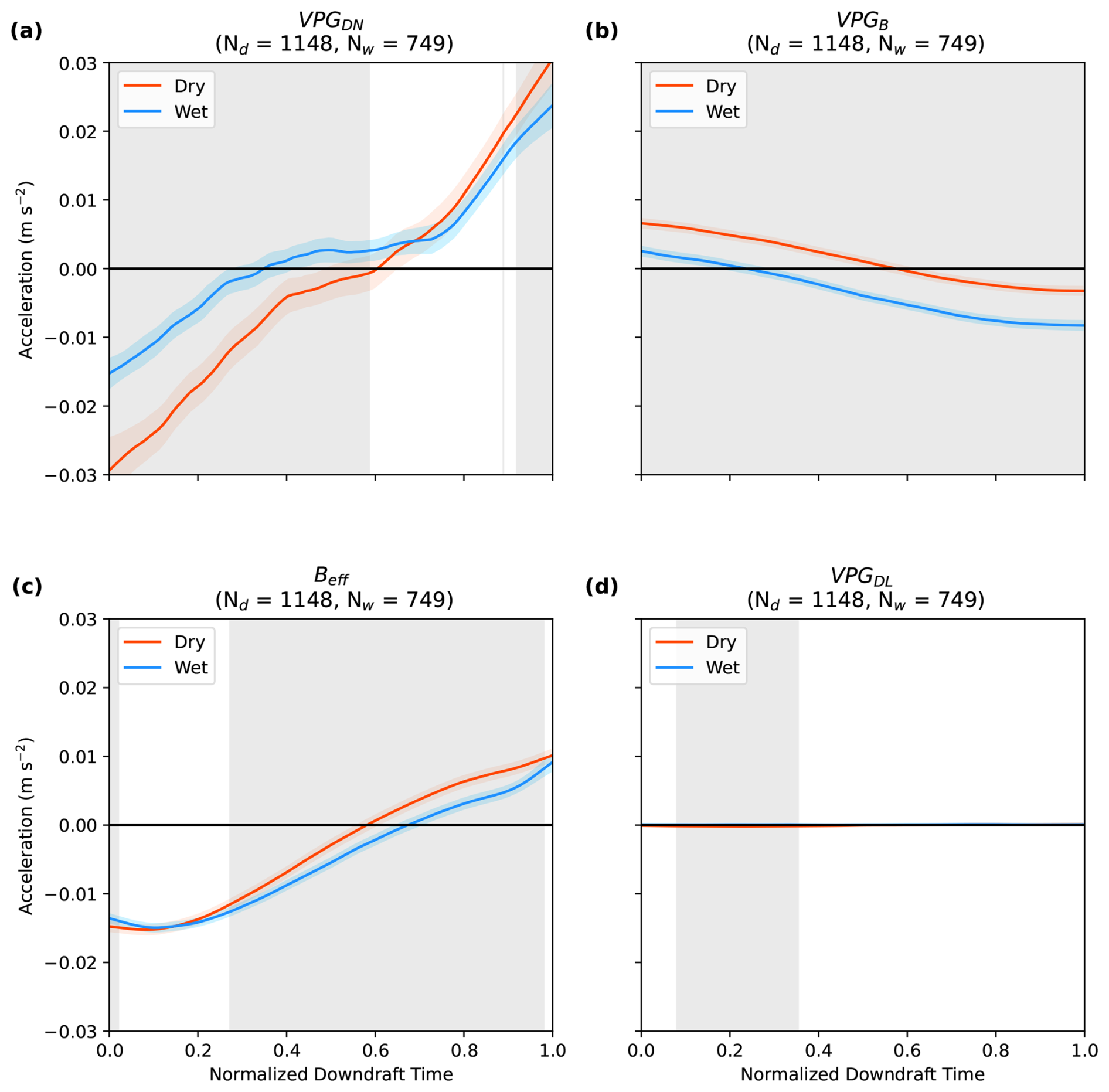
The parcel buoyant $\left({\mathrm{VPG}}_B=-c_p{\mathit{\theta }}_{\mathit{\rho },\mathrm{0}}\frac{\partial {\mathit{\pi }}_B^{\prime }}{\partial z}\right)$, dynamic linear $\left({\mathrm{VPG}}_{\mathrm{DL}}=-c_p{\mathit{\theta }}_{\mathit{\rho },\mathrm{0}}\frac{\partial {\mathit{\pi }}_{\mathrm{DL}}^{\prime }}{\partial z}\right)$, and dynamic nonlinear $\left({\mathrm{VPG}}_{\mathrm{DN}}=-c_p{\mathit{\theta }}_{\mathit{\rho },\mathrm{0}}\frac{\partial {\mathit{\pi }}_{\mathrm{DN}}^{\prime }}{\partial z}\right)$ contributions to VPG accelerations in both simulations are plotted in Fig. 8. Effective buoyancy (B_eff; i.e., the net thermodynamic acceleration; Davies-Jones, 2003), which is simply the sum of B and VPG_B, is also plotted to show the effect that pressure perturbations have on modulating B. VPG_DN has the largest magnitude of the three decomposed perturbation pressure accelerations. The temporal evolution of VPG_DN closely mimics that of the total VPG. Initially VPG_DN drives strong downward acceleration, but undergoes a sign reversal and drives strong upward acceleration by the end of the downdraft lifetimes. The magnitude of the initial downward VPG_DN is considerably larger in the dry simulation than in the wet simulation, suggesting that this pressure contribution largely explains the differing total VPG magnitudes seen in Fig. 7c. Wet simulation VPG_B begins as positive but quickly becomes negative 20 % into the downdraft, contributing downward acceleration thereafter. In contrast, the VPG_B in the dry simulation remains positive for ≈ 55 % of the downdraft, becoming negative thereafter. Such VPG_B accelerations partially counteract the strong negative B that arises from cloud edge evaporative cooling, while also opposing the positive B that decelerates downdraft parcels once they have descended below their levels of neutral B. Consequently, B_eff shows a similar increasing trend like B itself, but magnitudes are reduced at the origin and termination points of the downdraft compared to B. In fact, B_eff magnitudes are reduced from B to a greater extent in the dry simulation than in the wet because dry simulation VPG_B is positive for more of the downdraft. This counteracts the difference in B between the simulations, leading to similar B_eff magnitudes. VPG_DL is very small relative to the other VPG contributions, which is likely a result of relatively weak vertical wind shear in both simulations (Fig. 1). This pressure contribution does not contribute to the differing overall VPG magnitudes seen in Fig. 7c.

Previous subsiding shell studies have noted the presence of downward acceleration just within the cloud edge as well, where in-cloud negative B may be present (e.g., Katzwinkel et al., 2014; Nair et al., 2020; Savre, 2021). To ensure that the accelerations shown in Figs. 7–8 are representative regardless of shell definition, we applied the same analysis to a new set of identified shell points, where w<0 m s⁻¹ and total cloud water mixing ratio was allowed to exceed 0.01 g kg⁻¹. Total non-cloud hydrometeor mixing ratio was also restricted to be less than 0.01 g kg⁻¹ in order to filter out any in-cloud hydrometeor-loaded downdrafts. However, as was done previously, points were only classified as shell points if they were in the vicinity of the cloud boundary. After identifying the parcels that passed through these new shell points, parcel w, VPG, B, and total acceleration were gathered (Fig. 9).

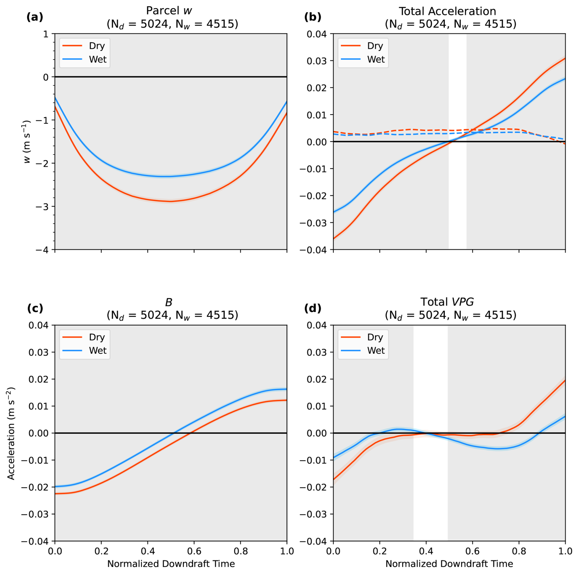
Figure 9 Same as Fig. 7, but for in and out-of-cloud subsiding shell points. Parcel w was added to the figure as panel (a).

With in-cloud points included as shell points, mean shell parcel w magnitude decreases, especially in the dry season (Fig. 9a). Such weakening of subsidence is due to a substantial decrease of the VPG contribution, specifically in the VPG_DN term. Such decrease could arise due to the increased parcel sample size, but it is also possible that pressure gradients are slightly stronger on the outside of the cloud versus inside. Despite the VPG magnitudes de-amplifying, B becomes more negative throughout the downdraft. Aligned with previous literature mentioning negatively buoyant cloudy air, it appears as though many of the new points and parcels identified are cloudy and negatively buoyant, leading to the greater contribution to subsidence from B. This negative buoyancy arises from injection of environmental air into the cloud and the resulting evaporation/sublimation of a high volume of cloud water or ice. Despite the changes in subsiding shell w from the acceleration magnitude variation, the general behaviors of both resolved and subgrid accelerations are the same. Therefore, whether in-cloud downdraft points are included or not, the accelerations driving subsiding shells are the same, regardless of shell definition.

Following Peters et al. (2019), we ascertain the net (i.e., integrated) contribution of each of these accelerations to downdrafts. This is accomplished by first considering the frictionless vertical velocity equation:

$$\begin{array}{}\text{(7)}& {\displaystyle \frac{\mathrm{d}w}{\mathrm{d}t}}=B+\mathrm{VPG}+SG,\end{array}$$

where SG represents acceleration from subgrid scale processes. We may use the chain rule to re-write the left-hand-side term as $\frac{\mathrm{d}w}{\mathrm{d}t}=\frac{\mathrm{d}w}{\mathrm{d}z}\frac{\mathrm{d}z}{\mathrm{d}t}=w\frac{\mathrm{d}w}{\mathrm{d}z}=\frac{d}{\mathrm{d}z}\frac{w^{\mathrm{2}}}{\mathrm{2}}=\frac{\mathrm{dKE}}{\mathrm{d}t}$, where $\mathrm{KE}\equiv \frac{w^{\mathrm{2}}}{\mathrm{2}}$ is the kinetic energy. Upon vertically integrating from the downdraft start height z_i to any arbitrary height below the start height z, we obtain:

$$\begin{array}{}\text{(8)}& {\displaystyle }\mathrm{\Delta }{\mathrm{KE}}_B\left(z\right)=\underset{z^{\ast }=z_i}{\overset{z^{\ast }=z}{\int }}B\mathrm{d}{z}^{\ast },\text{(9)}& {\displaystyle }\mathrm{\Delta }{\mathrm{KE}}_{\mathrm{VPG}}\left(z\right)=\underset{z^{\ast }=z_i}{\overset{z^{\ast }=z}{\int }}\mathrm{VPGd}{z}^{\ast },\text{(10)}& {\displaystyle }\mathrm{\Delta }{\mathrm{KE}}_{\mathrm{SG}}\left(z\right)=\underset{z^{\ast }=z_i}{\overset{z^{\ast }=z}{\int }}\mathrm{SGd}{z}^{\ast },\text{(11)}& {\displaystyle }\mathrm{\Delta }{\mathrm{KE}}_{\mathrm{tot}}\left(z\right)=\mathrm{\Delta }{\mathrm{KE}}_B\left(z\right)+\mathrm{\Delta }{\mathrm{KE}}_{\mathrm{VPG}}\left(z\right)+\mathrm{\Delta }{\mathrm{KE}}_{\mathrm{SG}}\left(z\right),\end{array}$$

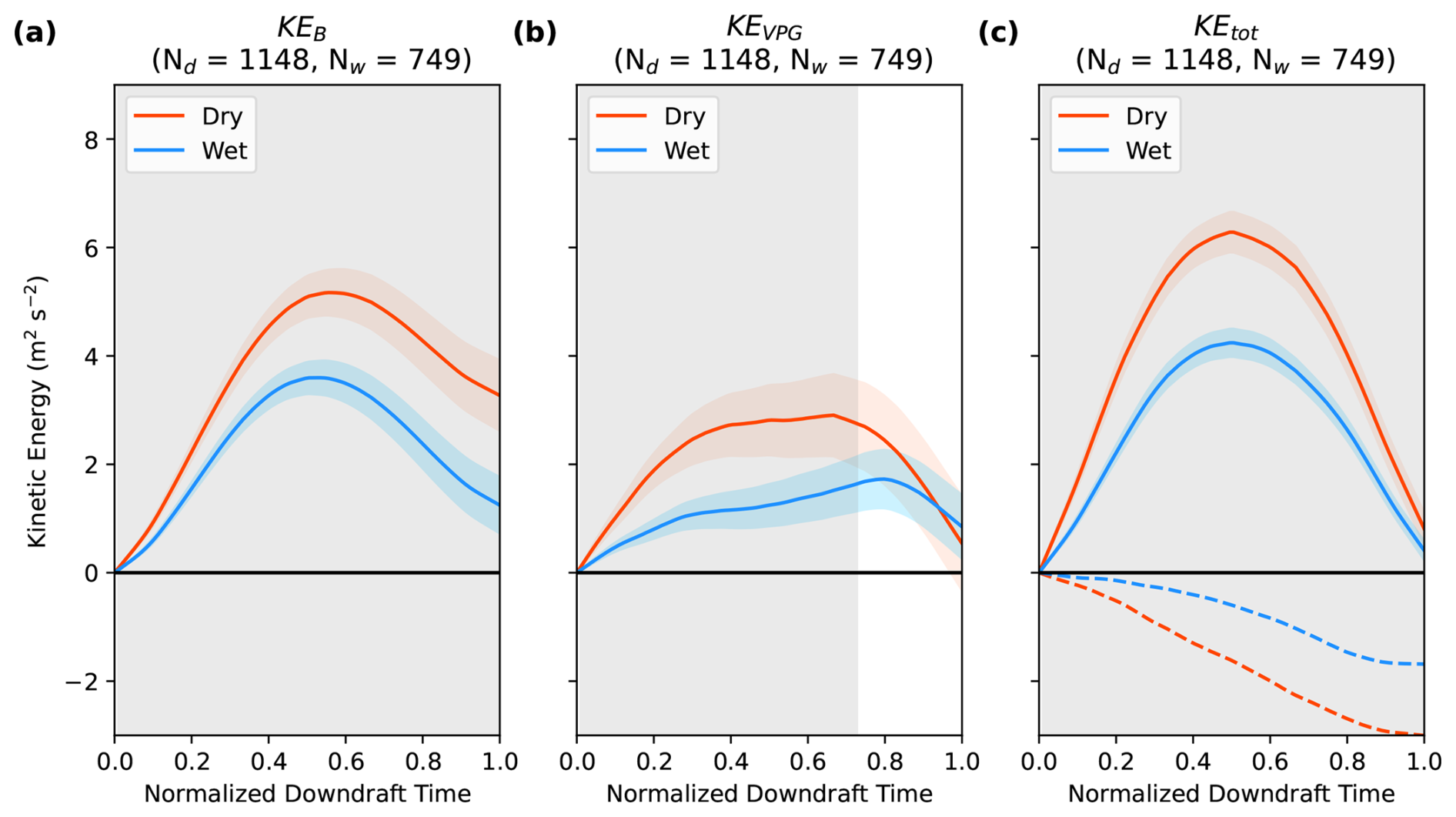
where ΔKE is the change in kinetic energy between the parcel's starting location z_i and a given height below the starting point z and z^∗ is a dummy variable of integration. We similarly compute ΔKE_VPG,B, ΔKE_VPG,DL, ΔKE_VPG,DN, and $\mathrm{\Delta }{\mathrm{KE}}_{B_{\mathrm{eff}}}$. Note that despite downward velocities within a downdraft, the absolute change in KE is positive since w is squared. Processes that accelerate the parcel downward will contribute positive ΔKE, whereas parcels that accelerate the parcel upward will contribute negative ΔKE. With the assumption that KE(z_i)=0 at the downdraft start, all ΔKE terms can be expressed as KE. Throughout the downdraft, KE_tot is larger in the dry simulation than the wet (Fig. 10c) because downdraft speeds are more negative in the dry than in the wet simulation. Both KE_B and KE_VPG contribute meaningfully to total KE, though KE_B (Fig. 10a) is roughly double that of KE_VPG (Fig. 10b) in both simulations. Hence, downdrafts in our simulations are both buoyantly and dynamically driven, though B is the predominant contributor. Both KE_B and KE_VPG are larger in the dry simulation by roughly equal magnitudes. This means that while B is the predominant overall driver of shell downdrafts, the environmental differences in downdraft strength are roughly equally driven by differences in B and differences in the VPG. The dampening of total KE from subgrid scale turbulence can also be seen in Fig. 10c where KE_SG is negative.

Figure 10 Same as Fig. 7, but for parcel KE.

Figure 11 Same as Fig. 10, but for (a) KE_VPG,DN, (b) KE_VPG,B, (c) ${\mathrm{KE}}_{B_{\mathrm{eff}}}$, and (d) KE_VPG,DL.

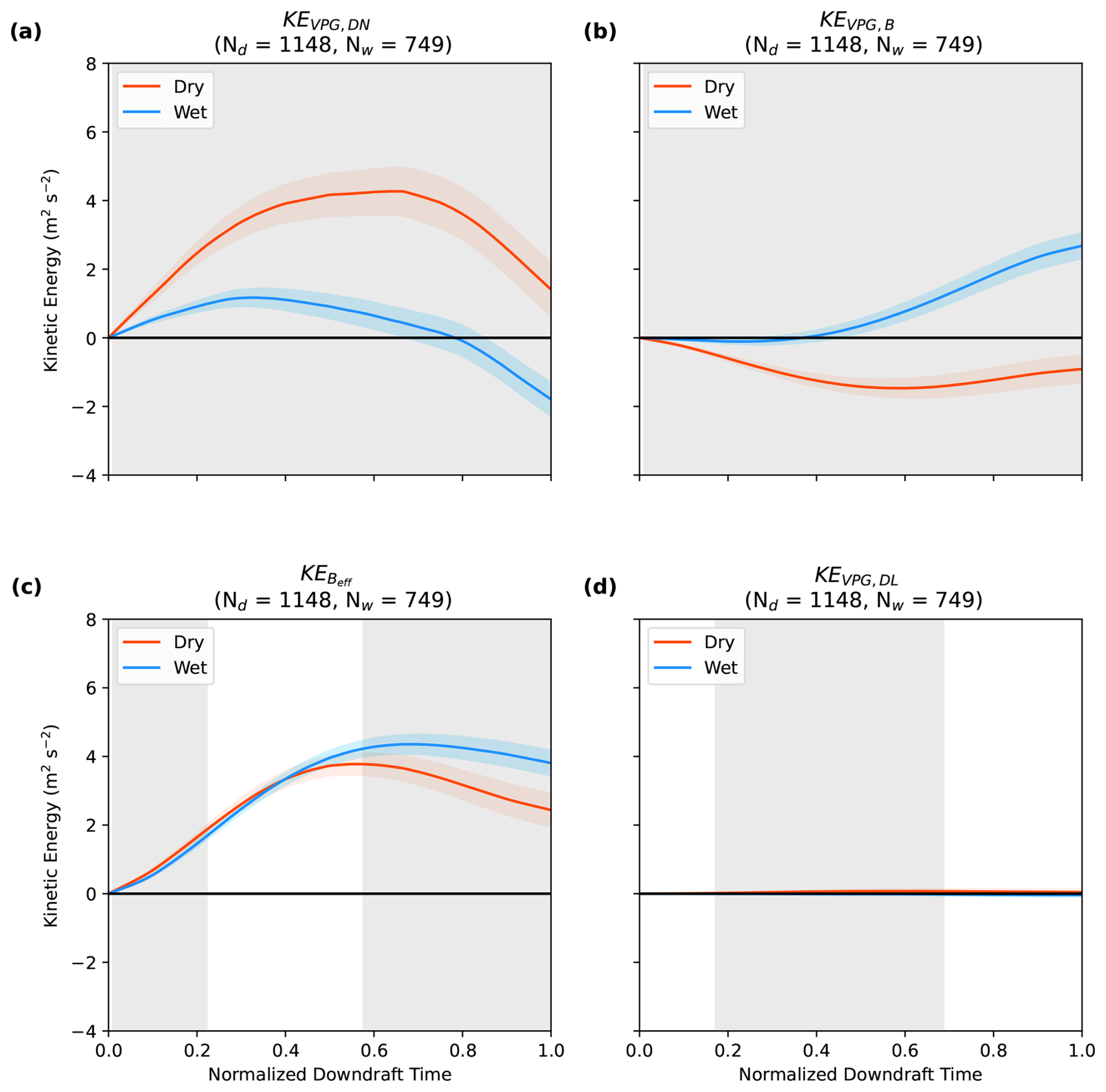
The results in Fig. 10 support both of the hypotheses proposed in the introduction that larger negative B and larger downward dynamic pressure accelerations drive stronger downdrafts in the dry season than in the wet season. However, an examination of ${\mathrm{KE}}_{B_{\mathrm{eff}}}$ and KE_VPG,B calls this conclusion to question. Specifically, the appreciably larger KE_B in the dry season simulation is largely offset by smaller KE_VPG,B in the dry season simulation, such that the difference in ${\mathrm{KE}}_{B_{\mathrm{eff}}}$ between the wet and dry season simulations is small (Fig. 11c). This implies that while downdrafts are more negatively buoyant in the dry season, the atmosphere's thermodynamic response to these more negatively buoyant downdrafts induces an upward pressure gradient acceleration that nearly entirely offsets this larger negative B. Hence, the differences in downdraft strength between the wet season and dry season are predominately driven by larger KE_VPG,DN in the dry season than in the wet season (Fig. 11a). In other words, there is stronger dynamic forcing for downdrafts in the dry season. Furthermore, ${\mathrm{KE}}_{B_{\mathrm{eff}}}$ is now comparable in magnitude to KE_VPG,DN, implying that shells are roughly equally thermodynamically and dynamically forced.

3.3 Congestus Versus Deep Shells

Exploration of shell origin and termination heights prompted a comparison between shells associated with shallow/congestus cumulus and deep convection (Fig. 12). A bimodal distribution appeared in both the origin and termination heights, with a peak in origin heights centered about 9000 and 8000 m in the dry and wet season, respectively, but also at around 3000 m in both simulations. Termination height peaks in the distribution are shifted downward by about 500–1000 m, roughly matching the displacement magnitudes. Such displacement magnitudes are similar to those found in Hernandez-Deckers and Sherwood (2016), who looked at ascending thermals with a limited displacement due to drag supplied by nonhydrostatic pressure perturbations. In the case of our descending motion within the shell, we believe displacement is limited partially by the overshooting of the level of neutral buoyancy by parcels, and primarily by the upward-directed VPG_DN. We speculate that the bimodal distribution in shell origin/termination heights is associated with the congestus and deep regimes of cumulus. Given the large difference in the heights, it is possible that shell properties for congestus and deep convection may be different, especially since RH values are higher in the lower troposphere and the updrafts of congestus clouds are weaker. For this comparison, we assume cumulii that have a cloud top greater than 5 km are considered deep (Jensen and Genio, 2006), whereas any cloud below this height and above 2 km is categorized as congestus. Mean w of parcels passing through (a) deep and (b) congestus shells is shown in Fig. 13. Unsurprisingly, the mean w magnitude of deep parcels is greater in the deep convection shells than it is in the congestus shells. Deep shell parcels attain minimum w of −3.66 and −2.96 m s⁻¹ in the dry and wet simulations, respectively. In the congestus regime, dry parcel subsidence is 1 m s⁻¹ weaker than in the deep and wet parcel subsidence is only slightly reduced to −2.44 m s⁻¹.

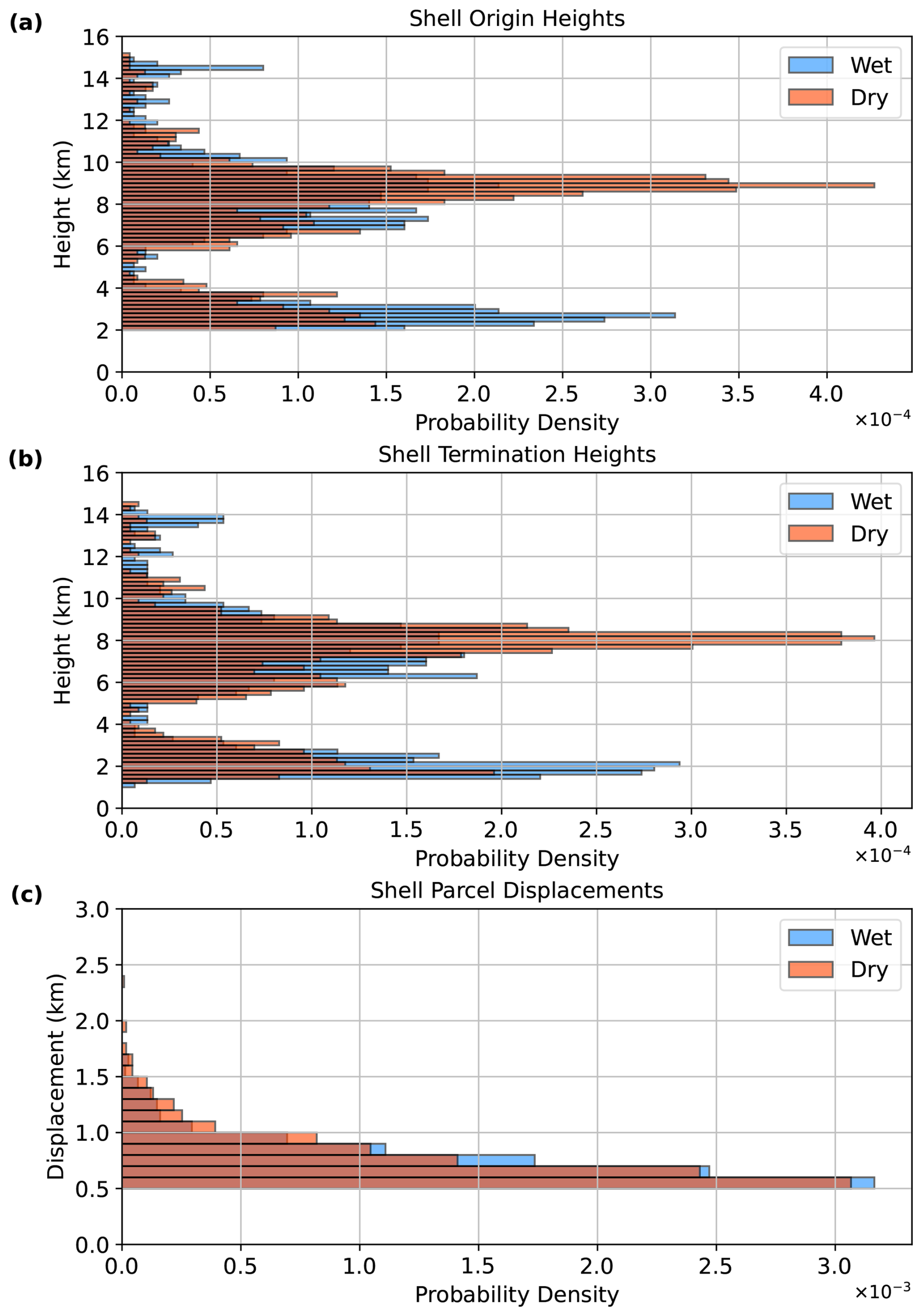
Figure 12 Probability density histograms for wet and dry simulation shell parcel (a) origin and (b) termination heights. Panel (c) shows displacement of the shell parcels for both simulations.

Figure 13 Same as Fig. 6, but for (a) deep and (b) congestus regimes of convection.

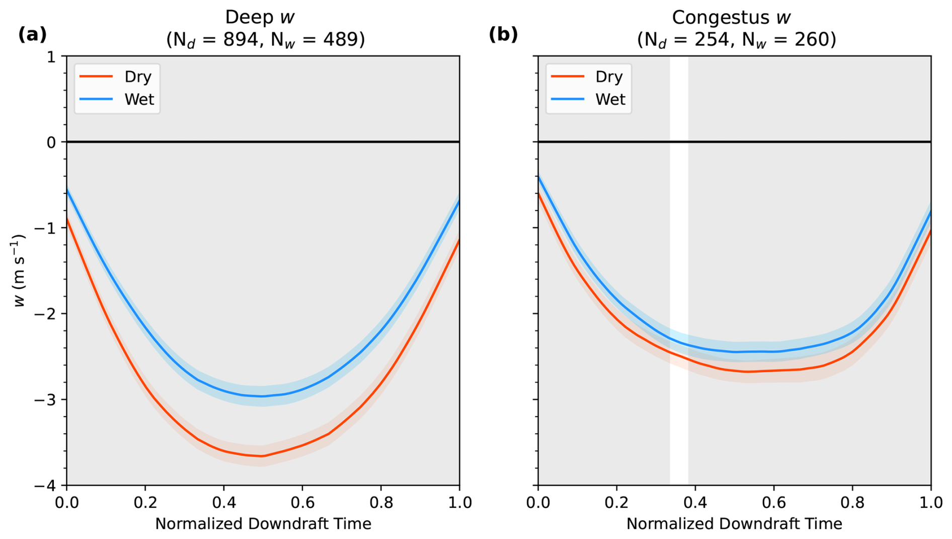
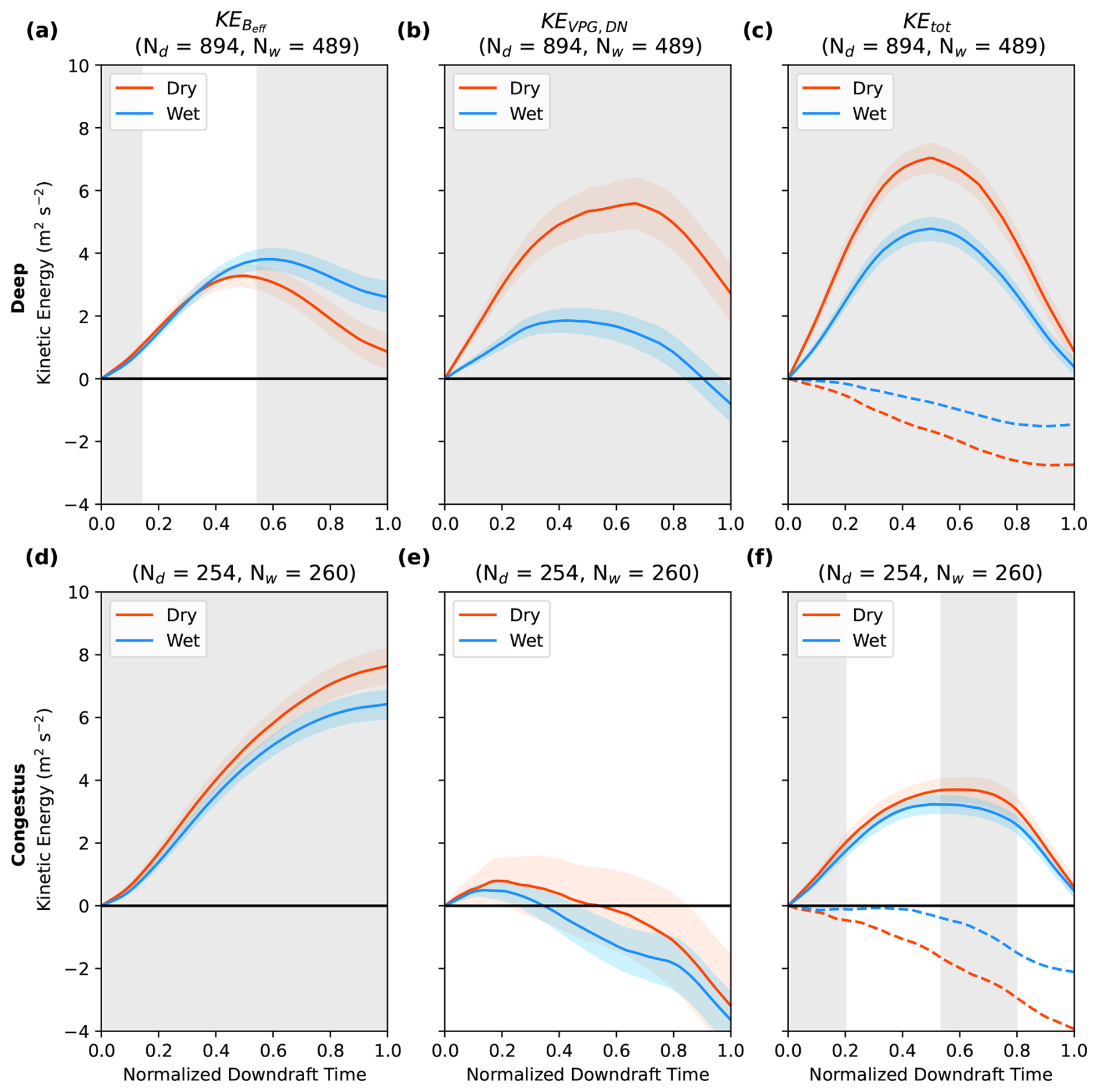
Figure 14 Same as Fig. 10, but for (a, d) ${\mathrm{KE}}_{B_{\mathrm{eff}}}$, (b, e) KE_VPG,DN, and (c, f) total acceleration for (a–c) deep and (d–f) congestus regimes of convection.

With differing w magnitudes between the two types of convection, we again perform an assessment of KE contributions to gauge the importance of thermodynamic and dynamic accelerations in shells. Figure 14 shows the comparison between deep and congestus contributions to KE from B_eff and the VPG_DN, as well as total acceleration with the subgrid contribution included. As was the case with w, maximum KE is greater in the deep shells versus the congestus shells (Fig. 14c, f). Additionally, in both convective regimes, dry simulation KE is greater at all times compared to the wet simulation. Given the larger number of parcels embedded within deep shell downdrafts, the behavior of KE in this regime is similar to that of all downdrafts combined (Fig. 10). With this being the case, attention turns toward the congestus regime, where KE contributions from B_eff and VPG_DN differ from their deep counterparts. Maximum total KE in congestus shells is reduced from that in deep shells in both simulations, with dry and wet congestus shells on average having 43.9 % and 24.5 % less KE than deep shells, respectively. Despite ${\mathrm{KE}}_{B_{\mathrm{eff}}}$ more than doubling in the dry simulation, total KE decreases. This is due to the overpowering effect of KE_VPG,DN, which decreases significantly and is largely negative for much of the downdraft in the congestus regime. A large subgrid contribution exists in the dry simulation as well, again due to stronger updrafts in that simulation. Magnitudes of wet simulation differences in individual accelerations are reduced, with both ${\mathrm{KE}}_{B_{\mathrm{eff}}}$ increasing and KE_VPG,DN decreasing only minimally. With this, it is clear that VPGs are generally weaker (and potentially more detrimental) in congestus shells than they are in deep convection shells. Furthermore, KE_VPG,DN is not statistically different between the dry season and wet season congestus shells, implying that the more intense downdrafts in dry congestus shells are primarily driven by these shells being more negatively buoyant in the dry season. This contrasts with deep convective shells, which were primarily stronger in the dry simulation because of a stronger downward VPG_DN.

3.4 Physical processes contributing to accelerations

Visualization of the shell structures in both simulations and the two modes of convection was done via compositing of shells. The composites of subsiding shells allow us to physically interpret the processes driving the shells, and to understand how these processes differ between the two simulations. As shown in the previous section, differences may arise in the properties of shells associated with deep versus congestus convection. Shell width is one of those properties, and the widths of the shells that were used in the compositing process are shown in Fig. 15. Despite a mean deep convective shell width of 800 m identified in Savre (2021), the shells in the present study's simulations are much narrower. Dry simulation deep and congestus shells have mean widths of 480 and 420 m, respectively. Mean values are the same in the wet simulation, meaning shell width primarily depends on the depth of the convection. These low width values are surprising given that the updrafts in this study are deeper and stronger than those in Savre (2021). The congestus shell widths align with the findings of that study, but the deep shell widths are nearly half of their noted deep shell average. However, this reported average was specifically taken from cloud top, and Savre (2021) noted that widths of shallow and deep shells were fairly similar away from the very top of the cloud. With this, shells in deeper convection are slightly wider, but the magnitude more closely matches the mean shell width found away from the very top of the cloud (see Fig. 4 in Savre, 2021).

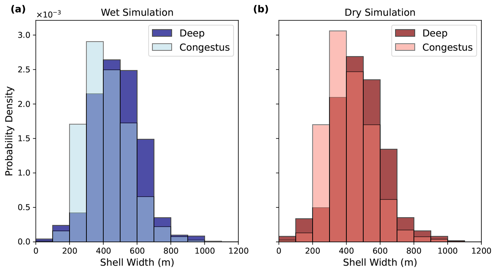
Figure 15 Probability density histograms for the widths of (a) wet and (b) dry simulation subsiding shells. Widths were sampled from all shells identified in the compositing process. Deep and congestus histograms are dark and light colors, respectively.

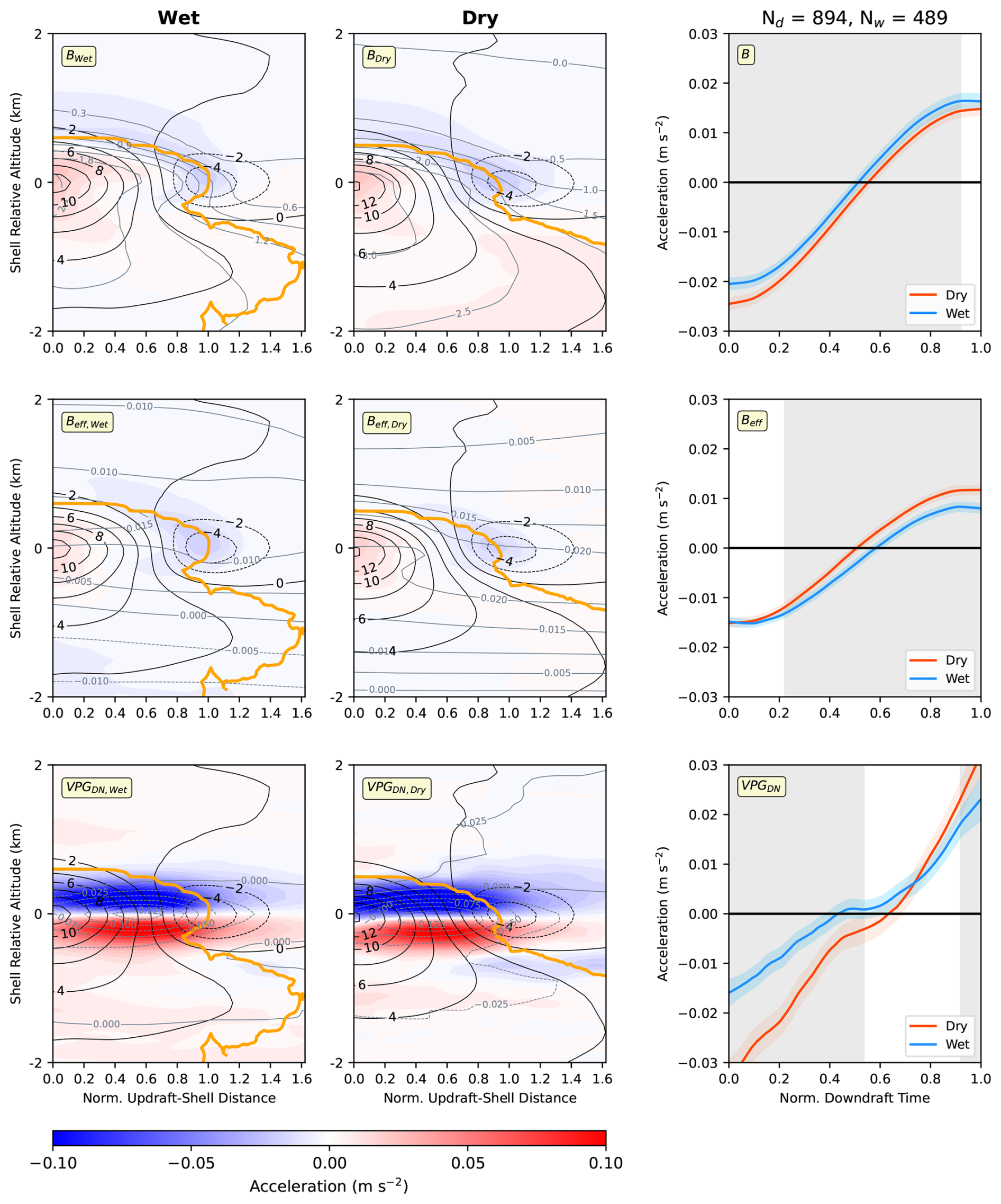
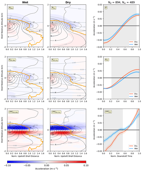
Figure 16 Wet (left column) and dry (middle column) simulation composites of subsiding shell downdrafts for the deep regime of convection. The vertical axis is the height (in km) relative to the height of the shell minimum w, and the horizontal axis is the fractional distance between the maximum w at the height of shell minimum w and the shell minimum w itself. Composites of B (top), B_eff (middle), and VPG_DN (bottom) are filled, and simulation parcel trajectories for these accelerations are shown in the right column. w is depicted in black contours, and $q_{\mathrm{v}}^{\prime }$ (top; in g kg⁻¹), ${\mathit{\pi }}_B^{\prime }$ (middle) and ${\mathit{\pi }}_{\mathrm{DN}}^{\prime }$ (bottom) are contoured in grey. ${\mathit{\pi }}_B^{\prime }$ and ${\mathit{\pi }}_{\mathrm{DN}}^{\prime }$ are scaled by 10³. Median cloud edge ($q_{\mathrm{c}}+q_{\mathrm{i}}=\mathrm{0.01}$ g kg⁻¹) is contoured in orange.

Figure 16 displays composited deep convective shells and their associated accelerations. Though composites of w show shells of similar strength, the parcel trajectory analysis supports stronger shells in the dry simulation. One potential reason for not seeing a stronger shell in the dry composite is the asymmetrical nature of shells and potential smearing from that variability. Therefore, it is crucial that the composites are interpreted as a visual for general updraft-shell structure. Focusing on B in Fig. 16, a clear region of negative B encapsulates a strongly positively buoyant updraft core. Negative B exists both above the updraft and on the flank of the updraft where shells are present. Such negative B may arise in two ways. The negative B existing above the updraft arises from the adiabatic cooling of environmental air that is pushed upward by an ascending thermal. Here, negatively buoyant parcels are forced horizontally toward the flanks of the updraft and can begin to sink down the edges of the cloud in the shell. However, stronger negative B exists where shell subsidence is maximized. It is here that a strong positive perturbation of q_v is present, likely owed to the evaporative cooling of cloud droplets at the edge of the updraft. The presence of this feature in the composite supports the evaporative cooling mechanism of formation of subsiding shells (e.g., Heus and Jonker, 2008). When comparing B to B_eff, the region of downward acceleration that was located above the updraft is eliminated and only that which occurs in the shell remains. Because B_eff accounts for the effects of VPG_B, and with a high ${\mathit{\pi }}_B^{\prime }$ perturbation found in the upper portions of the updraft, almost all downward acceleration from negative B above the updraft is offset by upward VPG_B, leading to no downward acceleration in this region. Therefore, all subsidence only will occur on the flanks of the updraft in the shell where negative thermal B arising from evaporative cooling dominates.

While a clear horizontal dipole in the B and B_eff structure exists between the shell and the updraft, a vertical dipole is present in the VPG_DN field and is maximized where vertical gradients of ${\mathit{\pi }}_{\mathrm{DN}}^{\prime }$ are largest. The ${\mathit{\pi }}_{\mathrm{DN}}^{\prime }$ field is structured so that a minimum in pressure is found embedded within the maximum horizontal gradient of w. This is also where the horizontal B gradient is maximized, allowing the minimum in pressure to arise in the center of the toroidal circulation associated with rising cloud thermals. As seen in both the composites and parcel trajectory accelerations, this VPG_DN dipole structure leads to a downward acceleration above the shell core, and a positive acceleration below it. Additionally, the magnitude of VPG_DN is much greater than that of B or B_eff. This is especially the case where shell subsidence originates, about 500 m above the region of maximum subsidence. It is here that parcels are essentially “sling-shotted” down the side of the cloud by the downward branch of the toroidal circulation, which acts as the driver of shell subsidence (e.g., Savre, 2021).

The dependence of downward shell accelerations on the toroidal low pressure regions explains why VPG_DN is more intense in the dry simulation than in the wet simulation. That is, the magnitude of the toroidal low should scale with the magnitude of updraft w and the horizontal B gradient within the cloud core. This connection between w and ${\mathit{\pi }}_{\mathrm{DN}}^{\prime }$ is evident in the analytic solutions of Hill and Henrici (1894), and is further shown in simulations of moist thermals in Morrison and Peters (2018) (see Eq. 13 in that study). Hence, the dry simulations have stronger downdrafts than the wet because the dry simulations have stronger overall updrafts and consequently stronger downward accelerations driven by toroidal low pressure (Marion and Trapp, 2019).

Figure 17 Same as Fig. 16, but for the congestus regime.

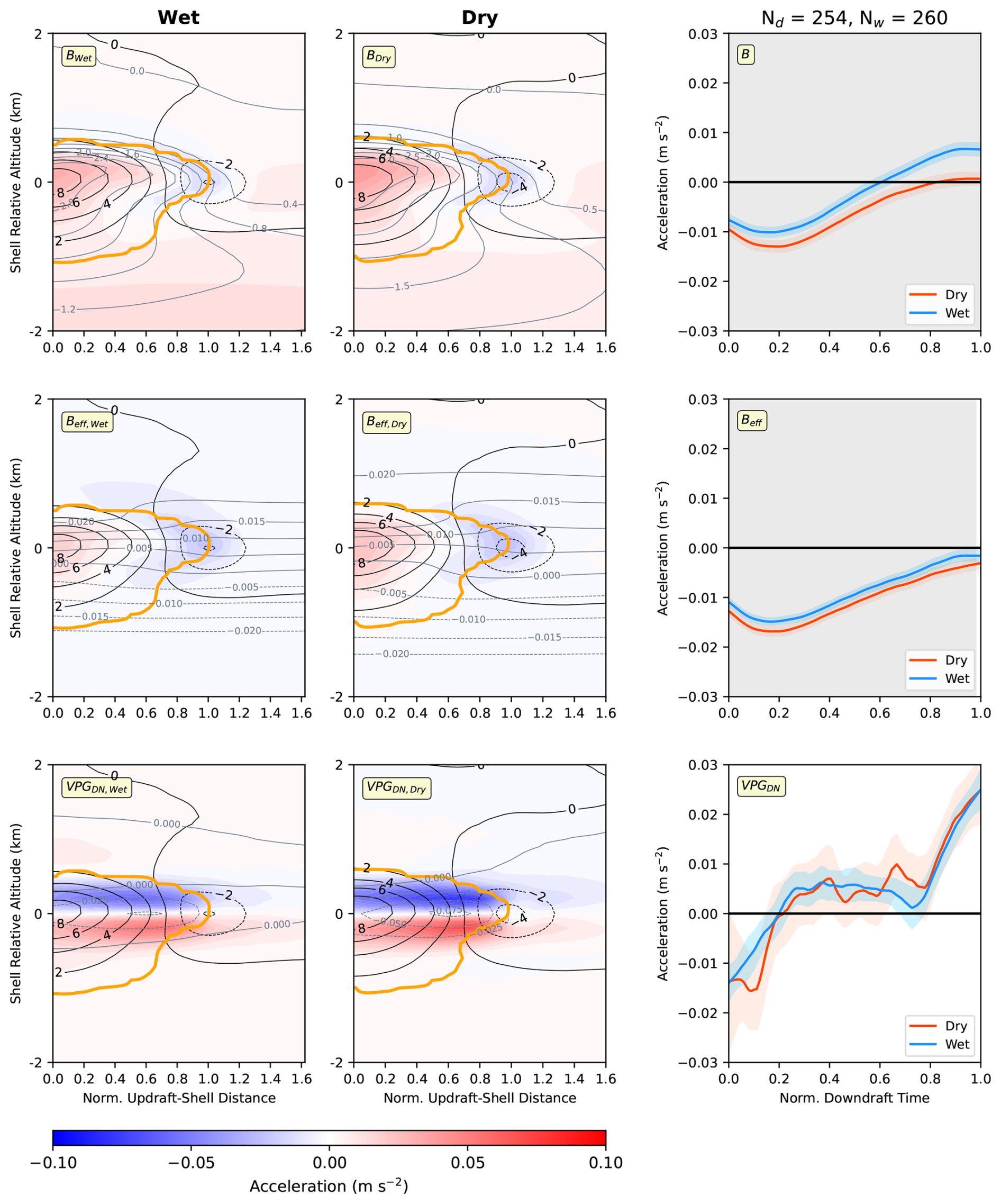
The structure of the w field in the congestus regime composite (Fig. 17) is similar to that of the deep composite, aside from the congestus updrafts being weaker. The most notable differences between the deep and congestus composites is associated with the shell features. Congestus composite negative B and B_eff wrap around the updraft in a bean-like shape, and negative values in these features extend further downward than they do in the deep convection composites. The trajectories support this, with negative buoyant accelerations persisting in the downdraft period longer than in the deep shells. Therefore, it is likely that the congestus regime exhibits more of the evaporative cooling processes that occur at cloud edge, which is supported by slightly stronger $q_{\mathrm{v}}^{\prime }$ in the congestus shells than the deep shells. Though B variations are present between the two regimes, the most notable differences is embedded within the VPG_DN fields. The composite structure of congestus VPG_DN is nearly identical to that of deep convection, but magnitudes are reduced. This comes as no surprise as the strength of the VPG_DN is proportional to horizontal B gradients and updraft strength, and such gradients and updrafts are weaker in the congestus convection. The weakened negative VPG_DN prevents shells from being as strong as those in the deep regime.

To summarize (e.g., Fig. 18) parcels near cloud top are first accelerated downward by the VPG_DN induced by the toroidal circulation and by negative B driven by the evaporation of condensates. Because this circulation is proportional to updraft strength and horizontal B gradients, the VPG_DN is stronger in deep convection versus shallow convection, and in stronger dry season simulations than in the wet season simulations. As soon as parcels within the shell pass below the height of minimum ${\mathit{\pi }}_{\mathrm{DN}}^{\prime }$ in the toroidal circulation, they experience an upward VPG_DN acceleration and only B_eff and momentum can maintain the subsidence. Parcels will also become more positively buoyant as they overshoot their levels of neutral B. Once parcels are well below the height of minimum ${\mathit{\pi }}_{\mathrm{DN}}^{\prime }$ and are positively buoyant, shell subsidence ceases. Based on both Fig. 12 and the composites, such processes yielded shells that were only about 500–1500 m in depth, depending on the strength of the convection. The authors note that individual cloud structures are much more complex than that shown in Fig. 18, as well as the composites of deep and congestus convection (see Fig. 4). Heterogeneity among clouds will likely lead to inter-cloud differences in shell strength and behavior, likely due to the alteration of B and VPG magnitudes. However, given that shells are primarily driven by these two accelerations, the composites in Figs. 16–17 are an effective representation of the entire subsiding shell population. Additionally, shell downdrafts may not necessarily begin at cloud top, as depicted in Fig. 18. Investigation of individual parcels revealed most subsiding shell downdrafts originated above a thermal, whether it be at cloud top or potentially a rising thermal near the base of the cloud. Such thermals may be present at different stages of a cloud's lifetime, which may have implications on the relative contributions of each acceleration to shell subsidence. The link between subsiding shell properties and cloud life stage will be investigated in the future.

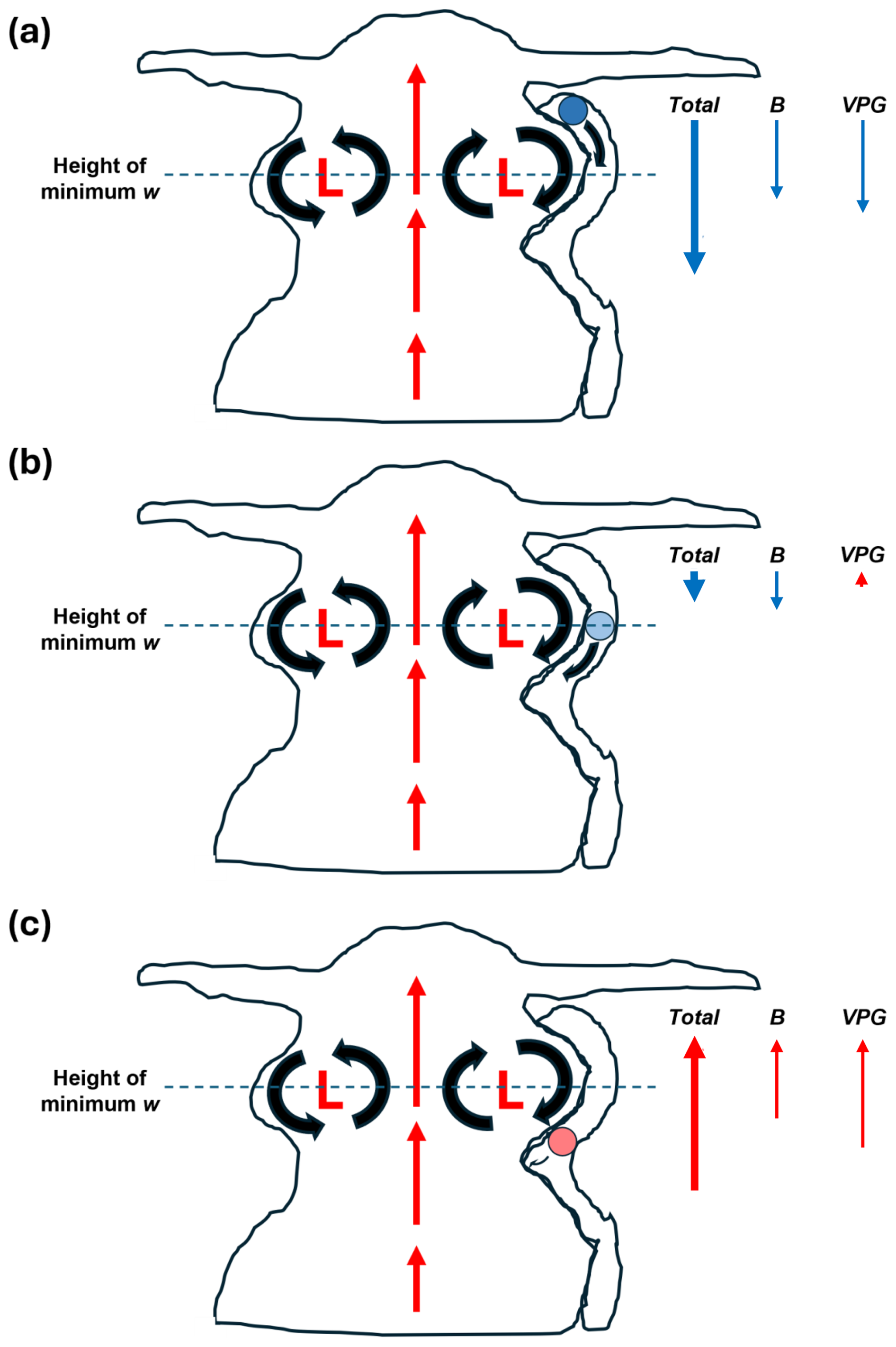
Figure 18 Schematic diagrams of parcel (colored circle) descent through a subsiding shell at cloud edge (contoured in black at cloud edge) when it is (a) above a thermal, (b) at its minimum w, and (c) below a thermal. Parcel color is blue when negatively buoyant and red when positively buoyant. Thermal circulations are denoted by bold black arrows around thermal-induced low pressure (depicted with L). Deep convective updrafts are denoted with red arrows passing through the center of the cloud. Accelerations (total, B, and VPG) are shown to the right of the cloud, and signs and relative magnitudes of the accelerations are implied with direction and length of the arrows.

4 Conclusions

This study investigated the influence of environmental RH on subsiding shells in deep moist convection using LES and a Lagrangian parcel trajectory analysis. Two LESs were initialized with atmospheric profiles representing the convective regimes of the wet season and the dry season in the Amazon. The primary difference between these two atmospheric profiles was larger middle free-tropospheric RH in the wet season than in the dry season, which facilitates a systematic assessment of the influence of RH on subsiding shell behavior. After completion of this assessment, the following conclusions were made regarding shell characteristics:

1. Both negative buoyancy from evaporative cooling and flow deformation, as well as dynamic perturbation pressure accelerations associated with thermally-driven toroidal circulations drive shell subsidence.

2. Subsiding shells are stronger in the drier environment not because of greater evaporative cooling rates, but because updrafts and their resultant dynamic perturbation pressure accelerations are stronger. This highlights the large dependency of shell strength on updraft strength.

3. Despite a greater contribution from negative buoyancy, congestus convection has weaker subsiding shells than deep convection due to a significantly reduced contribution from dynamic pressure accelerations.

Shell parcels were typically displaced downward by roughly a kilometer, with maximum negative w on the order of 2–4 m s⁻¹. Lagrangian parcel analysis reveals that the shells were driven by both negative effective buoyancy resulting from condensate evaporation and downward oriented dynamic pressure accelerations driven by the low pressure regions within the toroidal circulations of cloud thermals. Descent in downdrafts ceased once parcels overshot their level of neutral buoyancy and passed below the toroidal low, after which B became positive and the pressure gradient acceleration became oriented upward. Throughout the downdraft, subgrid scale turbulent accelerations also contributed to drag, potentially due to the mixing of updraft or environmental air into the shell.

Consistent with radar observations of the wet season and dry season in the Amazon (e.g., Giangrande et al., 2023), downdrafts in subsiding shells were significantly stronger in the dry season than in the wet season. While dry season shells intuitively experienced larger negative buoyancy than their wet season counterparts because of greater condensate evaporation in a drier lower free troposphere, this difference was largely counteracted by a larger upward oriented buoyancy pressure acceleration in the dry season. Hence, while large and downward in both simulations, the effective buoyancy was similar in dry season and wet seasons. In contrast, downward oriented dynamic pressure accelerations were significantly stronger in the dry season simulation which explains this simulation's stronger downdrafts. This occurred because updrafts were stronger in the lower-to-middle troposphere in the dry season owing to steeper low-level lapse rates and smaller entrainment rates, which resulted in stronger toroidal low pressure in rising cloud thermals. With this, the hypothesis motivated by Giangrande et al. (2023) concerning the link between updraft strength and downdraft response is confirmed. Though greater rates of evaporative cooling may have been found at cloud edge, utilizing an effective buoyancy framework exhibited limited difference in buoyancy between the two seasons, implying that any increased evaporative cooling in the dry season is canceled out by a counteracting buoyancy pressure acceleration.

Dividing convection into deep and congestus regimes showed that magnitude and behavior of the accelerations driving subsiding shells is also dependent on cloud properties. Deep convective subsiding shells were much stronger than their congestus counterparts due to an increased contribution from the dynamic pressure accelerations. These larger pressure contributions arose because the deep convective updrafts were stronger, leading to an increase in toroidal circulation strength and its associated pressure gradient acceleration. Interestingly, despite having weaker updrafts and pressure accelerations, a greater impact from negative effective buoyancy arose in the congestus regime. This was likely the result of a weaker buoyant pressure acceleration coupled with more persistent evaporative cooling through the depth of the shell. Such a result emphasizes the importance of treating subsiding shells differently in shallow versus deep convection rather than assuming shells are driven by one primary mechanism for all clouds.

Though subsiding shell accelerations are driven by both negative buoyancy and pressure perturbations, we emphasize that such acceleration behavior and magnitude is strongly tied to subgrid scale choices such as the selected microphysics scheme. Shell identification itself is based on cloud edge, which is determined based on the number concentration of cloud water and cloud ice. Additionally, the magnitude of negative buoyancy from evaporative cooling is directly linked to number concentration, particle size distribution, and the magnitude of mixing from the subgrid turbulence scheme as well. With all this, selection of subgrid parameterization schemes must be taken with care, as acceleration magnitudes are at least partially dependent on these choices.

Increasing vertical wind shear would also change the characteristics of the shells. As discussed in Heus and Jonker (2008), the presence of strong wind shear led to shallow cumulus shell asymmetry, with subsidence only existing on the downshear side of the cloud. This shell region was wider and collocated with a region of high relative humidity downshear of the cloud (Heymsfield et al., 1978; Laird, 2005; Heus and Jonker, 2008). In this study's simulations of deep convection, a similar mechanism could arise if shear were to increase. The tilting of clouds, which would predominately be the case for the congestus regime, would likely lead to the shell asymmetries discussed in Heus and Jonker (2008). Shells associated with wider and deeper updrafts may undergo similar changes if the magnitude of the shear was large enough to significantly tilt the updrafts. Additionally, how the increase of shear affects updraft strength should be considered. As has been shown in studies such as Peters et al. (2020), an increase in shear is directly correlated with wider, less diluted updrafts that can have a larger maximum vertical velocity. With this, if vertical velocity of updrafts increases in response to the shear increase, then dynamic nonlinear pressure perturbation accelerations may prove to be larger. A stronger updraft would also lead to more horizontal shearing from turbulence at cloud edge, which could increase mixing, evaporative cooling, and negative buoyancy. Therefore, it is fair to hypothesize that increasing the vertical wind shear could have both a direct impact on shell asymmetry, as well as an indirect impact on shell strength via an alteration of the updraft properties.

Subsiding shell downdrafts play a crucial role in the transport of mass, heat, and momentum in the tropical atmosphere, all of which must be accurately assessed to maximize the accuracy of a climate model. Therefore, it is necessary that the driving mechanisms behind such shells are understood and applied to models. In addition to investigating the effects of environmental RH on shell behavior, it is recommended that steps be taken to properly implement subsiding shell and other near-cloud downdraft effects into cumulus and convective parameterizations. To do this, future work points to investigating shells in a variety of environments, including those in a strongly-sheared environment. Leveraging observations of deep convective subsiding shell properties may also prove beneficial, such as those acquired during the Experiment of Sea-breeze Convection, Aerosol, Precipitation, and Environment (ESCAPE) field campaign (Kollias et al., 2025). This, coupled with the continuation of LES and other numerical simulations, will lead to better comprehension of subsiding shells and encourage implementation of shell dynamics into climate models.

Appendix A

With a majority of previous subsiding shell studies focused on shallow cumulus, many of which used finer horizontal and vertical grid spacing of 50 m or less (e.g., Heus and Jonker, 2008; Dawe and Austin, 2011; Nair et al., 2020). These shallow cumulus shells are much more narrow than that of deep convection, typically on the order of no more than 200 m wide (Katzwinkel et al., 2014; Savre, 2021), so finer grid spacing allows for proper resolution of these narrow shells driven by turbulent mixing and the aforementioned processes discussed in this study. Therefore, questioning of this study's 100 m grid spacing choice is certainly warranted. To address this concern, sensitivity tests of varying grid spacing were performed.

Because we wish to assess subsiding shell properties from a more statistical approach, we cannot simply focus on a high-resolution simulation of one cloud and its associated shell. We must allow for many shells to occur over a large domain representative of convective coverage in the tropics, so an LES of 50 m or less over this sizable of a domain would be extremely computationally expensive. With this, we cannot perform sensitivity tests by decreasing grid spacing down to 50 m. However, we are able to instead increase our grid spacing from the 100 m used in this study to upwards of 200 m. By doing this, we can compare the results of our 100 m simulation to that of coarser grid spacing and assess if the relative role of B, VPG, and subgrid-scale processes change. Attention will especially fall on the subgrid scale and B, as both of these contributions to acceleration are physically attributed to mixing processes at cloud edge.

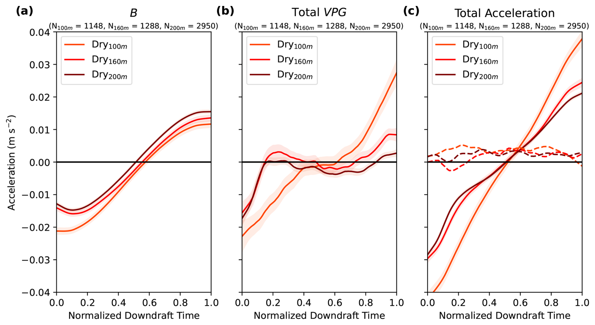
Two sensitivity simulations were performed with the exact model setup as that in this study, but with 160 and 200 m horizontal grid spacing, respectively. Such grid spacings were chosen to demonstrate the increasing importance of the subgrid turbulence parameterization as grid spacing decreases, which exhibits the impacts of mixing. All subgrid parameterizations, nudging, fluxes, and initiation were unchanged. An analysis of subsiding shells was again performed in the final hour of the simulation when 30 s trajectory and model output were available. Mean parcel w trajectories are shown in Fig. A1. As grid spacing is increased towards 200 m, the strength of dry season subsiding shells decreases. Such an alteration of shell strength occurs due to differences in the shell accelerations, which are shown in Fig. A2. Evidently, coarsening the grid spacing did not significantly impact the behavior of the accelerations, but rather reduced the amplitude of them. As such, the subsiding shell vertical velocities in Fig. A1 are reduced. Parcel time series curves of B were shifted upward, while VPG behavior remained the same with a reduction in origin and termination acceleration magnitudes. Despite reductions in both the B and VPG, the total acceleration behavior remains unchanged. With this, it is evident that larger grid spacings have a “smoothening” impact on resolved accelerations, which would effectively weaken the shell. Therefore, if grid spacing was reduced from 100 m down towards 50 m, it is likely that more acceleration would be resolved, mainly in the form of B from resolved evaporative cooling at cloud edge, as well as VPG with enlarged gradients from dynamic nonlinear pressure perturbations associated with a better-resolved toroidal circulation. However, despite coarsening of the grid, the subgrid contribution from turbulence remains mainly constant, aside from the beginning of the shell downdrafts. Such differences do not follow a consistent change with grid spacing, but in all cases, the subgrid turbulence still acts to dampen the downward accelerations of the shells.

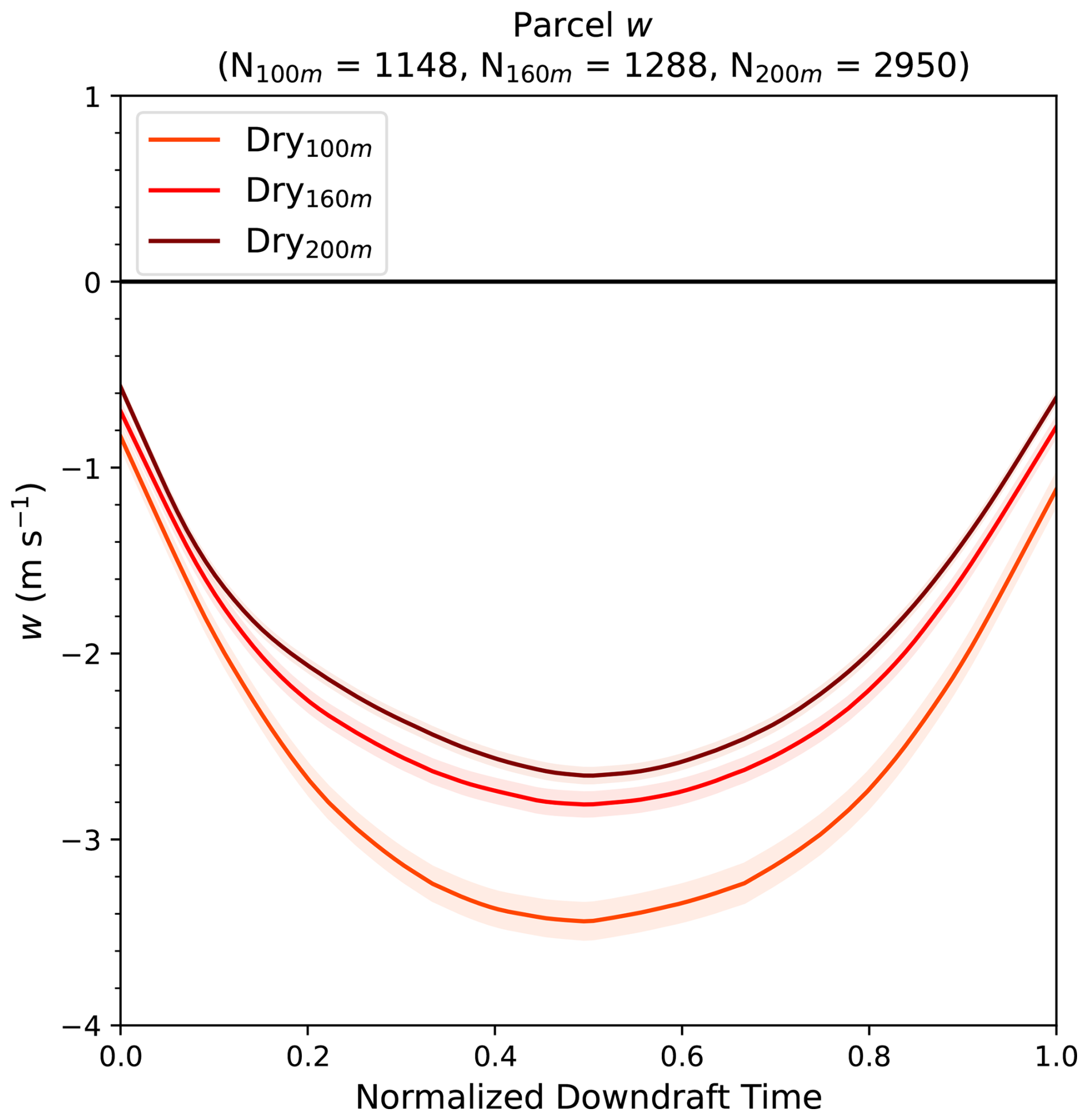
Figure A1 Same as Fig. 6, but for parcels in the 100 m (orange), 160 m (red), and 200 m (maroon) sensitivity simulations.

Figure A2 Same as Fig. 7, but for parcels in the 100 m (orange), 160 m (red), and 200 m (maroon) sensitivity simulations.