Consistent estimates of carbonyl sulfide and methane stratospheric lifetimes retrieved from AirCore profiles at different latitudes

Stratospheric loss is a major sink for both carbonyl sulfide (COS) and methane (CH₄), but their stratospheric lifetimes and sinks remain poorly constrained because high-resolution observations of their vertical distributions in the lower stratosphere are sparse. Here, we estimate the mean stratospheric lifetime and sink of COS and CH₄ from their correlations with N₂O using two distinct methods applied to AirCore vertical profile measurements from three Northern Hemisphere summer campaigns. From these profiles, we derive a COS stratospheric lifetime of 69–90 years, corresponding to a sink of 30–41 GgS yr⁻¹. For CH₄,we find a stratospheric lifetime of 149–168 years, corresponding to a sink of 23–26 TgC yr⁻¹. These values are in good agreement with previous estimates (39–76 years for COS, 152–160 years for CH₄) and with estimates based on ACE-FTS observations (75–76 years for COS, 146–172 years for CH₄). As has been noted previously, we also find a decline in the COS tropospheric burden between 2016 and 2020 in our AirCore samples, in contrast to the continued growth of CH₄ and N₂O. In addition, we found that tracer-tracer correlations vary among flights, and even within the same campaign, pointing to variability in lower-stratospheric composition. Although this variability may reflect differences in stratospheric transport, its origin remains unclear and requires further investigation. These results provide observational constraints on the stratospheric budgets of COS and CH₄ and help refine their representation in atmospheric chemistry and transport models.

1 Introduction

Carbonyl sulfide (COS or OCS) is the most abundant sulfur-containing gas species in the atmosphere, with a tropospheric mole fraction of 350–550 ppt (Remaud et al., 2023; Whelan et al., 2018). Following evidence of COS uptake in plants at leaf level, this species has been suggested as a proxy to separate gross primary productivity (GPP) from respiration in plants, to deepen the understanding of carbon exchange between atmosphere and vegetation (Stimler et al., 2010, 2012; Whelan et al., 2018). Some recent studies, however, observed bidirectional COS exchange in some species under drought conditions, which may complicate the application of this tracer as a GPP proxy (Cho et al., 2025; Spielmann et al., 2025). Moreover, recent studies evidenced a mismatch between models and observations, pointing towards unidentified or poorly quantified processes that may also contribute to COS uptake, which may also undermine its usefulness as a GPP proxy (Kaushik et al., 2026).

COS has a relatively long lifetime in the troposphere (2–2.5 years) (Montzka et al., 2007) and is therefore able to enter the stratosphere, primarily through tropical upwelling (Crutzen, 1976; Ma et al., 2021; Montzka et al., 2007; Remaud et al., 2023). In the stratosphere, it is converted to precursors of sulfuric acid (which is converted to stratospheric sulfate aerosols) by photolysis and by reactions with OH• and O• radicals (Brühl et al., 2012; Chin and Davis, 1995; Krysztofiak et al., 2015). However, the assessments of both the mass budget and the contribution of COS to the formation of the stratospheric aerosol layer have not found full agreement yet (Kremser et al., 2016; Krysztofiak et al., 2015; Wilson et al., 2008). So far, the efforts to measure stratospheric COS have been based on remote sensing techniques (Bernath, 2005; Boone et al., 2023; Glatthor et al., 2017; Hannigan et al., 2022; Leung et al., 2002; Toon, 1991; Velazco et al., 2011), whole air samples (Engel and Schmidt, 1994) or in-situ spectrometry (Gurganus et al., 2025; Kloss et al., 2019; Krysztofiak et al., 2015).

Methane (CH₄) is the second most important anthropogenic greenhouse gas in terms of radiative forcing, after carbon dioxide (CO₂) (Myhre et al., 2014). Its current tropospheric abundance is over 1900 ppb and has been constantly increasing in the past 20 years (Thoning et al., 2022). CH₄ is produced by both natural and anthropogenic sources. Among these, some of the major natural sources are wetlands, fresh waters and oceans, while the anthropogenic include livestock farming, agriculture, landfills and fossil fuels (Saunois et al., 2025). Its major sink is oxidation by OH• in the troposphere, which serves as a major source of background atmospheric CO (Lelieveld et al., 1998; Saunois et al., 2025). With an average atmospheric lifetime of about 9 years, CH₄ can enter the stratosphere (Rohs et al., 2006; Saunois et al., 2025), which acts as a CH₄ sink. There, this gas reacts with stratospheric-abundant oxidating species such as excited atomic oxygen, O(¹D), radicals such as OH•, or undergoes photolysis (Rohs et al., 2006). Moreover, stratospheric CH₄ chemistry affects ozone (O₃) concentrations and the oxidation of stratospheric CH₄ makes it the main sources of stratospheric water vapor (Han et al., 2025; Rohs et al., 2006). However, uncertainties in the magnitude of chemical loss of stratospheric CH₄ remain large due to variability in atmospheric transport and chemistry (Lelieveld et al., 1998; Portmann et al., 2012; Saunois et al., 2025).

Atmospheric lifetimes are useful quantities to assess the environmental impact of a gas species when emitted into the atmosphere (Volk et al., 1997). Typically, lifetimes are inferred from the ratio between the global total atmospheric burden of a species and its sinks. When estimating partial lifetimes with respect to stratospheric loss, the ratio is defined focusing only on stratospheric sink. For species with only stratospheric sinks, atmospheric and stratospheric lifetimes are equal (Brown et al., 2013; Volk et al., 1997), while for species such as COS and CH₄ these lifetimes do differ. In this study, we present estimates of COS average stratospheric lifetime and sink from observations performed at mid- and polar latitudes, inferred from their stratospheric correlation with nitrous oxide (N₂O) (Barkley et al., 2008; Engel and Schmidt, 1994; Karu et al., 2023; Krysztofiak et al., 2015; Plumb and Ko, 1992). The observations we use to infer stratospheric lifetimes are continuous vertical profiles with AirCore samplers (Karion et al., 2010; Zanchetta et al., 2026) combined with a Quantum Cascade Laser Spectrometer (QCLS, Aerodyne Research Inc., MA, USA, model TILDAS-CS). This technique allows the collection of continuous atmospheric profiles and their analysis with minimal preparation and treatment. The analysis on the QCLS allows for the simultaneous measurement of COS, N₂O, CH₄, CO₂ and CO. AirCore samplers were deployed in three different campaigns, namely Trainou (TRN, 47°58^′ N, 2°06^′ E), Kiruna (KRN, 67°53^′ N, 21°04^′ E) and Sodankylä (SOD, 67°22^′ N, 26°37^′ E). The lifetime estimates will be compared with ACE-FTS (Bernath, 2005; Boone et al., 2023; Velazco et al., 2011) spatially and temporally averaged observations, as well as with estimates from previous studies. We also present estimates of CH₄ stratospheric lifetime and sink inferred from the correlation between this gas species and N₂O in the stratosphere.

2 Datasets

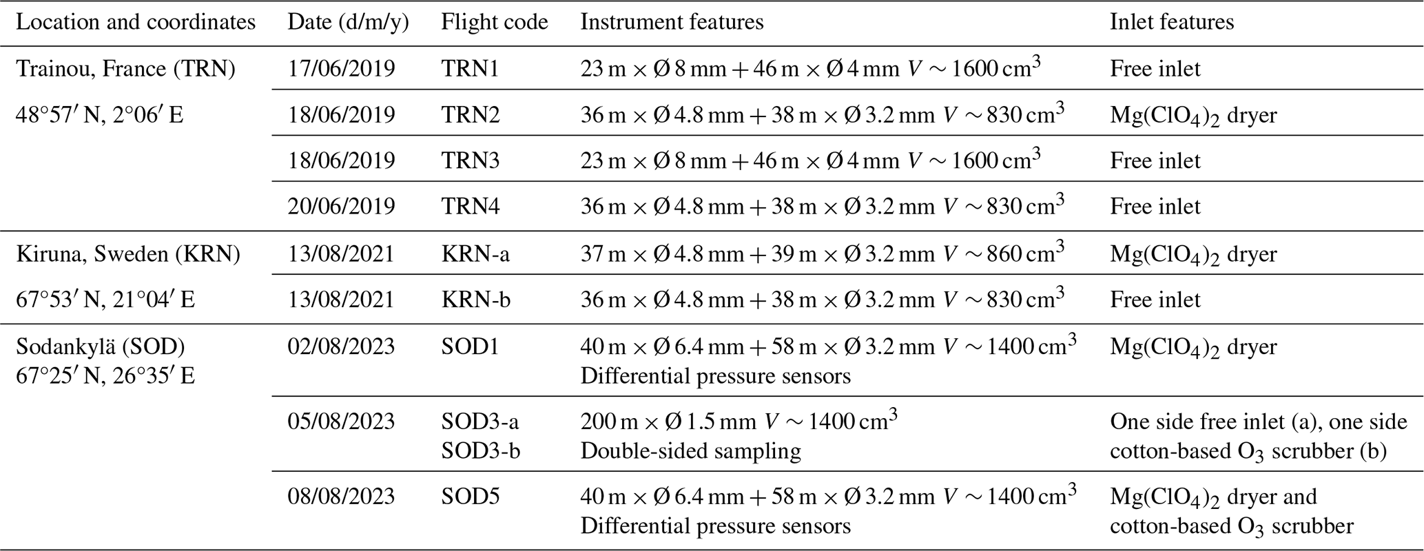
As thoroughly described in Zanchetta et al. (2026) and summarized in Table 1, AirCore samples were collected during three distinct balloon campaigns. The first campaign took place at mid-latitudes in Trainou (TRN, France), while the latter two were realized at polar latitudes in Kiruna (KRN, Sweden) and Sodankylä (SOD, Finland). Sampling, measurements and data processing will be briefly presented in the coming sections.

Table 1 Locations and dates of the performed sampling campaigns. The flight codes correspond to the ones presented in Zanchetta et al. (2026).

2.1 AirCore sampling

An AirCore sampler (Karion et al., 2010) consists of a coil made of stainless-steel tube, internally coated with Sulfinert^® (SilcoNert^® 2000) to minimize destructive interactions between steel and gas species. When deployed on stratospheric sounding balloons, it allows the passive collection of continuous vertical samples during the descent phase, thanks to the atmospheric pressure gradient (Karion et al., 2010; Membrive et al., 2017; Wagenhäuser et al., 2021). The sample is analyzed immediately after the flight on a continuous flow gas analyzer. Assuming pressure equilibrium, the pressure and temperature radiosonde readings can be used to calculate the sampled amount of air (in moles) for any time interval. Knowing the analyzed number of moles it is possible to link each aliquot to the sampling altitude and, therefore, retrieve the collected altitude profile (Karion et al., 2010; Membrive et al., 2017; Tans, 2022). These profiles can provide higher vertical resolution compared to remote sensing techniques (Gurganus et al., 2026). The profiles of this study were retrieved following the approach described in Membrive et al. (2017), except for the one collected with University of Bern's double-sided AirCore. One half of this AirCore was equipped with an O₂ injection system. The injections were programmed at specific altitudes (namely, at 21045.2, 17005.2, 11837.0, 7869.9 and 4592.2 m) to help the altitude retrieval process, similarly to the method described for CO in Wagenhäuser et al. (2021). These injections caused contamination spikes in the COS profile and were therefore visible in our analysis, which allowed the altitude retrieval process.

2.2 Quantum Cascade Laser Spectrometer (QCLS)

All AirCore samples have been analyzed on a dual laser QCLS (Aerodyne Research Inc., Billerica, MA, USA), an absorption spectrometer covering the mid-infrared (IR) frequencies range. Analysis of COS with mid-IR spectrometry was first described by Stimler et al. (2009). The instrument deployed in this study has been previously introduced in Vinković et al. (2022) and Tong et al. (2023). The QCLS measures CH₄, CO₂, N₂O, CO, COS and O₃ simultaneously and features a custom-made frontend, designed specifically for AirCore use. The operating parameters and the achieved measurement precision for each gas species are reported in Table S1 in the Supplement.

2.3 ACE-FTS observations

Similarly to Zanchetta et al. (2026), ACE-FTS observations were used as a validation tool of AirCore results. Conceptually, obtaining consistent results from two very different observational methodologies should provide proof of the reliability of both techniques. ACE-FTS is a satellite-borne spectrometer retrieving the altitude profiles of temperature, pressure and mole fractions of several gas species between 0–150 km altitude with a resolution of 1 km (Bernath, 2005; Glatthor et al., 2017; Velazco et al., 2011). The spectrometer retrieves profiles using solar occultation during sunset and sunrise. This limits the amount of measurable profiles, but enhances their vertical resolution (Bernath, 2005). Among its observations, ACE-FTS includes COS, N­₂O and CH₄, which allows the calculation of stratospheric lifetimes (Sect. 2.4). ACE-FTS observations showed strong agreement with recent in-situ high altitude COS observations (Gurganus et al., 2026). ACE-FTS v5.3 data (Boone et al., 2023) have been filtered to obtain a dataset complementary to the measured AirCore profiles. To stay close to the conditions of the campaigns, ACE-FTS observations of COS, N­₂O and CH₄ in summer months (June–September) after 2012 were selected between 45–49° N for Trainou and between 65–69° N for Kiruna and Sodankylä, respectively. The resulting 502 mid-latitude and 1681 polar latitude ACE-FTS profiles were averaged for each latitudinal interval. The resulting two averaged profiles (see Figs. 9 and 10 in Zanchetta et al., 2026) were then treated identically to the AirCore-derived profiles (as described in Sect. 3.1) to calculate COS and CH­₄ stratospheric lifetimes, and these mostly independent lifetime estimates are compared in Sect. 4.

3 Methods

3.1 Calculation of stratospheric lifetimes according to Plumb and Ko (1992)

Plumb and Ko (1992) described a method to calculate the stratospheric lifetime of a tracer. While for species with purely stratospheric sink the stratospheric lifetimes derived in this way are equal to the global lifetimes, they are only partial lifetimes for species with additional sinks in the atmosphere. The method further requires species to be in steady state and show an identifiable linear correlation in the lower stratosphere. If these conditions are met and the stratospheric lifetime of one species is known, then it is possible to calculate the stratospheric lifetime of another tracer, following:

$$\begin{array}{}\text{(1)}& {\displaystyle \frac{T_{\mathrm{1}}}{T_{\mathrm{2}}}}\cong {\displaystyle \frac{\mathrm{d}{\mathit{\sigma }}_{\mathrm{2}}}{\mathrm{d}{\mathit{\sigma }}_{\mathrm{1}}}}\cdot {\displaystyle \frac{{\mathit{\sigma }}_{\mathrm{1}}}{{\mathit{\sigma }}_{\mathrm{2}}}}\end{array}$$

where T_x is the stratospheric lifetime of a tracer, σ_x a mole fraction representative of the tracer's atmospheric abundance, and $\mathrm{d}{\mathit{\sigma }}_{\mathrm{2}}\mathrm{d}{\mathit{\sigma }}_{\mathrm{1}}^{-\mathrm{1}}$ is the slope of the tracer-tracer correlation in the lower stratosphere. For simplicity, given the smaller stratospheric abundances of the tracers when juxtaposed to the tropospheric portion of their profiles, we assume that the ratio of the atmospheric mean mole fractions can be approximated by the ratio of representative tropospheric mean mole fractions.

This method has been used to estimate the stratospheric lifetime of COS in various studies (Barkley et al., 2008; Engel and Schmidt, 1994; Karu et al., 2023; Krysztofiak et al., 2015). Specifically, Barkley et al. (2008) and Engel and Schmidt (1994) calculated the COS lifetime using its correlation with CFC-12, while Karu et al. (2023) and Krysztofiak et al. (2015) used its correlation with N₂O. In this study, we will estimate the lifetimes of COS and CH₄ using their stratospheric correlations with N₂O. Rearranging Eq. (1), we obtain:

$$\begin{array}{}\text{(2)}& T_x\cong {\displaystyle \frac{\mathrm{d}{\mathit{\sigma }}_{{\mathrm{N}}_{\mathrm{2}}\mathrm{O}}}{\mathrm{d}{\mathit{\sigma }}_x}}\cdot {\displaystyle \frac{{\mathit{\sigma }}_x}{{\mathit{\sigma }}_{{\mathrm{N}}_{\mathrm{2}}\mathrm{O}}}}\cdot T_{{\mathrm{N}}_{\mathrm{2}}\mathrm{O}},\mathrm{with}x=\mathrm{COS},{\mathrm{CH}}_{\mathrm{4}}\end{array}$$

Each variable at the right-hand side of the equation has an uncertainty. These uncertainties were propagated into an overall uncertainty of the lifetime estimate. The methods used to estimate ${\mathit{\sigma }}_{x,{\mathrm{N}}_{\mathrm{2}}\mathrm{O}}$, $\mathrm{d}{\mathit{\sigma }}_{{\mathrm{N}}_{\mathrm{2}}\mathrm{O}}\mathrm{d}{\mathit{\sigma }}_x^{-\mathrm{1}}$ and $T_{{\mathrm{N}}_{\mathrm{2}}\mathrm{O}}$ as well as their associated uncertainties will be described in the following sections.

3.1.1 Tropospheric burdens

Previous studies estimating COS lifetime using the Plumb and Ko (1992) method used different approaches to define σ_COS. According to Plumb and Ko (1992), σ_x should be a representative tropospheric mole fraction value of the considered tracer. It is good to mention that the stratospheric lifetime of a tracer should result from the ratio of its global atmospheric burden and its stratospheric sink. However, since the species considered in this study are all long-lived and show similar features in terms of transport and kinetics, the ratio of their tropospheric burdens can be considered a rather good approximation of the ratio of their total atmospheric burdens. Previous studies adopted different estimates to represent the tracers' burdens. Engel and Schmidt (1994) arbitrarily adopted an average tropospheric value of 500 ppt. Similarly, Barkley et al. (2008) assumed a value of 500 ppt ± 20 %. Krysztofiak et al. (2015) estimated an average tropospheric mole fraction of 550 ± 40 ppt from their in-situ observations. In contrast to Plumb and Ko's (1992), Karu et al. (2023) calculated σ_COS as 415 ± 32 ppt by averaging their stratospheric COS mole fraction observations. Global COS measurements remain very sparse and therefore the uncertainties associated to the tropospheric COS burden remain generally high (Hu et al., 2021; Kaushik et al., 2026). In this study, to obtain representative tropospheric mole fractions for COS, N₂O and CH₄, we followed the approach described in Andrews et al. (2001), which was previously used in other studies on age of air estimations (Andrews et al., 1999; Boering et al., 1996). Andrews et al. (2001) defined the stratospheric boundary conditions of CO₂ by averaging 12-months running means from surface data collected in Mauna Loa (19° N, MLO) and American Samoa (14° S, SMO), delayed by two months. Similarly, we calculated these means for each campaign for COS, N₂O and CH₄ and we estimated each species' tropospheric burden consequently using the updated database of NOAA's data described originally in Montzka et al. (2007). The calculated average tropospheric mole fractions are presented in Fig. 1 (the plots show 12-months running means and their standard deviations only every 6 months, for clarity). While the increase of N₂O and CH₄ is evident over time, it is interesting to notice that COS mole fraction decreased between 2016 and 2020 and showed a general increase between 2020 and 2025 (Gurganus et al., 2026; Hannigan et al., 2022; Serio et al., 2023). The larger deviations observed for CH₄ around 1998 and for both N₂O and CH₄ around 2024 are due to unusually low mole fractions observed in SMO and do not affect the results of this study.

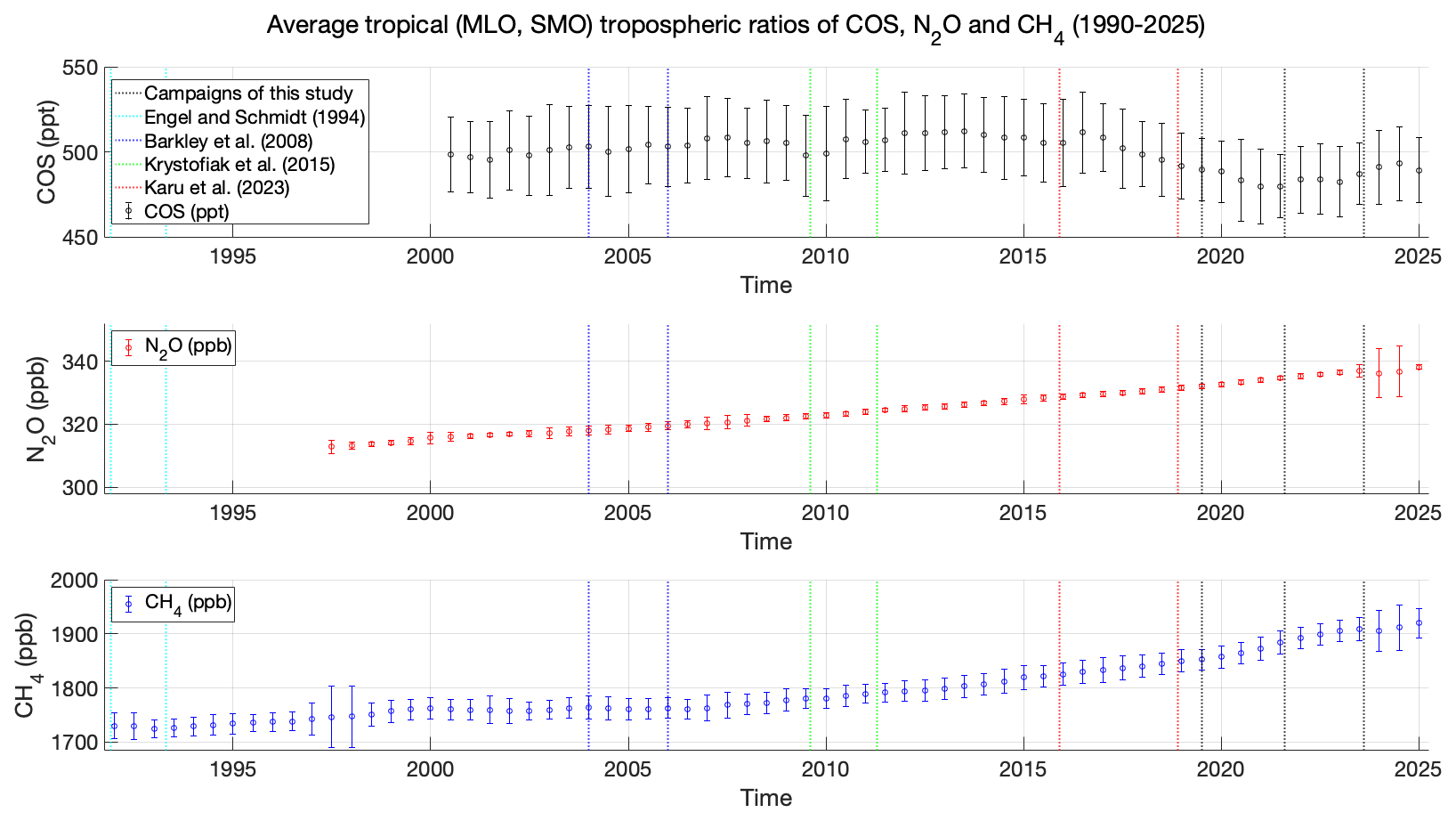
Figure 1 Averaged MLO and SMO tropospheric mole fractions retrieved from NOAA's flask observations, from which the burdens were derived. The vertical lines represent flight dates of different campaigns. For Barkley et al. (2008) and Karu et al. (2023), they represent the start and end of the periods covered by their campaigns.

3.1.2 Data selection for calculating the slope from tracer-tracer correlations

The stratospheric part of the profiles (Figs. 2a and 3a) was defined using the definition of thermal tropopause (WMO, 1957), calculating the lapse rate from the radiosonde data collected during each flight (Zanchetta et al., 2026). However, as exemplified in Figs. 2b and 3b, a non-linear relationship between COS (or CH₄) and N₂O was noticeable just above the thermal tropopause for all flights. Specifically, this deviation was observed in 2019 for N₂O mole fractions between 315 and 295 ppb, in 2021 between 310 and 325 ppb and in 2023 between 335 and 315 ppb. Likely, this is caused by a mixing of northern hemispheric tropospheric air with associated seasonality in both COS and CH₄ with stratospheric air in the lowermost stratosphere. This mixing would bias the regression analysis and consequently the final lifetime estimates. Therefore, the linear correlation was determined for N₂O mole fractions lower than 295 ppb in TRN, to 298 ppb in KRN and to 300 ppb SOD, progressively increasing the threshold to reflect the tropospheric increase of N₂O. Similar features, although smoothed, were also present in the averaged ACE-FTS correlations, which were therefore limited to N₂O mole fractions lower than 300 ppb. Plumb and Ko (1992) stressed the importance of limiting the tracer-tracer correlation analysis to mole fraction intervals where a linearity between both tracers is present. N₂O is a tracer of tropospheric origin with a stratospheric sink weak enough to make it long-lived throughout the lower stratosphere. If this condition is not fulfilled for another tracer, e.g. due to different stratospheric sinks (or sources) confined to specific stratospheric regions, the relationship between the species bends into a curve (see Sect. 4 in Plumb and Ko, 1992). In the collected AirCore samples, although there is no pronounced curvature, different linear relationships with COS can be found for N₂O mole fractions above and below 200 ppb (Fig. 2c), or above and below N₂O mole fractions of 230 ppb for CH₄ (Fig. 3c). These curvatures in the tracer-tracer relationships reflect different stratospheric chemistry over altitude affecting sources and/or sinks differently for each gas species (Plumb and Ko, 1992). Therefore, we limited the tracer-tracer correlations to the regions where a single-slope linearity between the species is respected, which corresponds to altitudes up to roughly 20 to 22 km. The two profiles obtained from SOD3 are cut at N₂O ≈ 280 ppb due to contamination effects (see Zanchetta et al., 2026). The details of the resulting selections are listed in Table S2 and the selection processes are illustrated in Supplement Sects. S1 (COS) and S2 (CH₄) in the Supplement for all flights except for TRN2 (in Figs. 2 and 3).

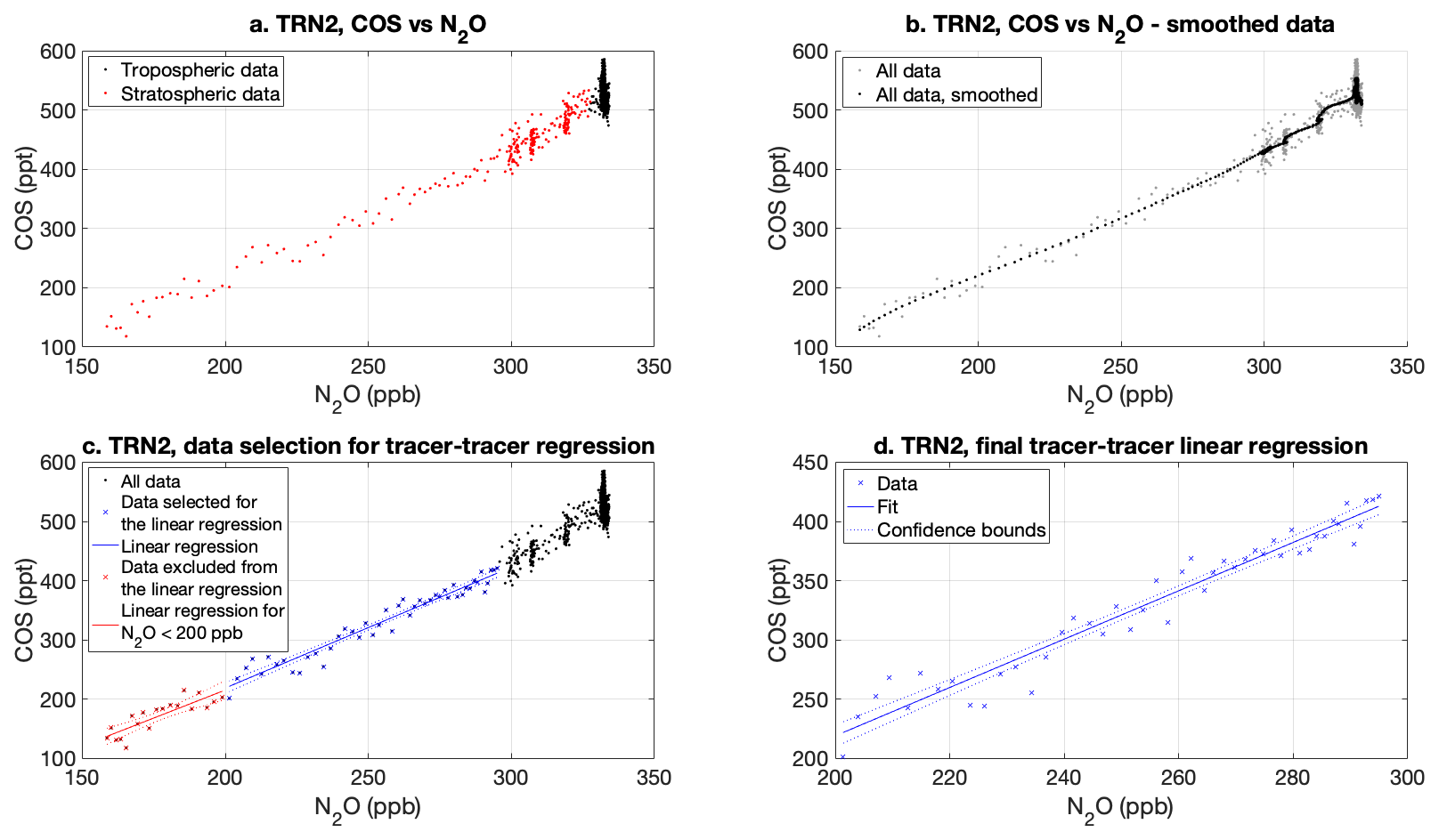
Figure 2 Data selection steps for the linear regression between COS and N₂O, exemplified with the TRN2 AirCore data.

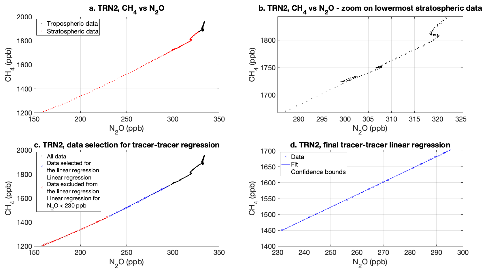
Figure 3 Data selection steps for the linear regression between CH₄ and N₂O, exemplified with the TRN2 AirCore data.

3.1.3 Data deficiency and flagging of outliers

Due to the data selection described in Sect. 3.1.2, the tracer-tracer correlation dataset for flight SOD3-b was restricted to a single data point. Therefore, it was not possible to retrieve a correlation with the profiles obtained from this flight.

Another AirCore flight (KRN-a) was marked as an outlier for COS. As shown in Table S3, the linear regression between N₂O and COS for KRN-a resulted in a much lower R² value and featured a much smaller slope than the other flights at polar latitudes did. Although in Zanchetta et al. (2026) the retrieved profile was comparable within uncertainties with previous stratospheric COS observations, between altitudes between roughly 17 and 20 km the profile was significantly lower than all other profiles (see Figs. 2, 6 and 8 in Zanchetta et al., 2026). Since the data selected for the tracer-tracer correlation falls in the same range, this has probably biased the results of the regression. Overall, the reason for this discrepancy remained unclear, but we speculate it may have been due to issues during the COS measurements, caused either by instability of the QCLS analyzer, or by contamination during sampling or analysis.

3.2 Calculation of stratospheric lifetimes following Volk et al. (1997)

The method of Plumb and Ko (1992), described in the previous section and adopted in several previous studies (e.g., Barkley et al., 2008; Engel and Schmidt, 1994; Karu et al., 2023; Krysztofiak et al., 2015) assumes steady state for both tracers, implying a globally uniform stratospheric correlation between the two species and no significant long-term tropospheric trends. Volk et al. (1997) applied a more comprehensive formalism to this theory, refining its boundaries while still applying Eq. (2). To account for deviation from the “slope equilibrium” of Plumb and Ko (1992), Volk et al. (1997) advocate the extrapolation of the tracer-tracer slope at the (extratropical) tropopause, where the correlation shall be representative of the tracers' vertical gradient. This would also prevent biases that may be observed (e.g., as curvatures in the tracer-tracer correlation slopes) due to non-diffusive mixing during transport from the tropics to mid latitudes. Moreover, this method requires global atmospheric burdens integrated over altitude, differently from the tropospheric burdens adopted by Plumb and Ko (1992). The procedures adopted to apply the Volk et al. (1997) method are described in Sect. 3.2.1–3.2.3. The assumptions on N₂O lifetime are identical for both methodologies (Sect. 3.3).

3.2.1 Global atmospheric burdens

To obtain a representative estimate of global atmospheric burdens of COS, N₂O and CH₄, their mean tropospheric mole fraction was firstly inferred following the method of Andrews et al. (2001), similarly to what has been described in Sect. 3.1.1. The obtained averaged tropospheric mole fractions were assumed to be constant up to 10 km of altitude. Above this altitude, to estimate the average global stratospheric mole fractions, ACE-FTS data at tropical, mid and polar latitudes were averaged for each campaign's year (2019, 2021 and 2023). Likewise, the average global pressure profiles were retrieved from ACE-FTS data for each year. Both the tropospheric average and the averaged stratospheric mole fractions were then multiplied by the corresponding average pressure at each altitude, summed together and divided by the total pressure, obtaining a global average burden weighted by the contribution of each atmospheric layer over altitude. An example of the mole fraction profiles against pressure, used to estimate the global atmospheric burdens, is presented in Fig. S19 in the Supplement.

3.2.2 Calculation of local stratospheric slopes and extrapolation of tracer-tracer slope at the tropopause

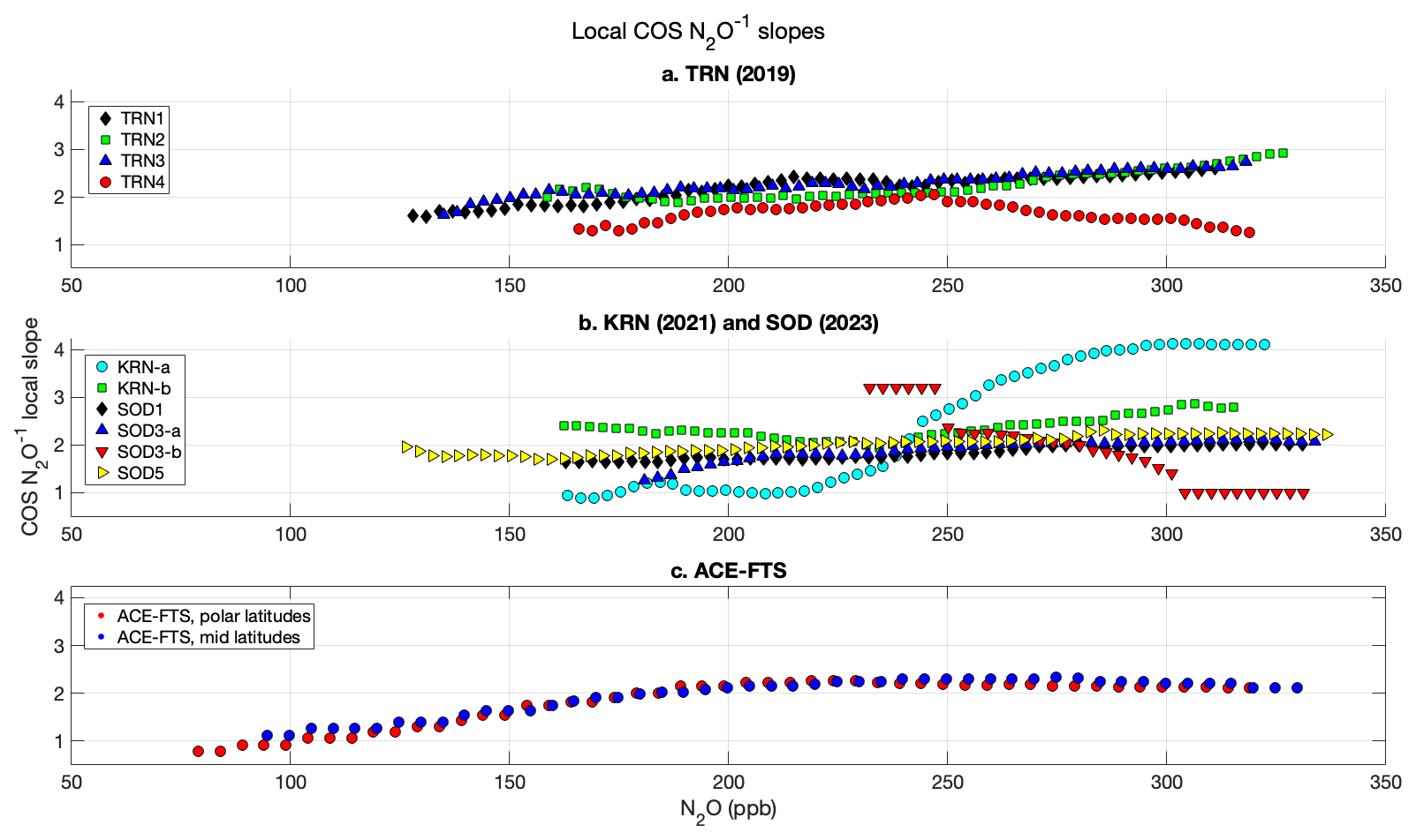
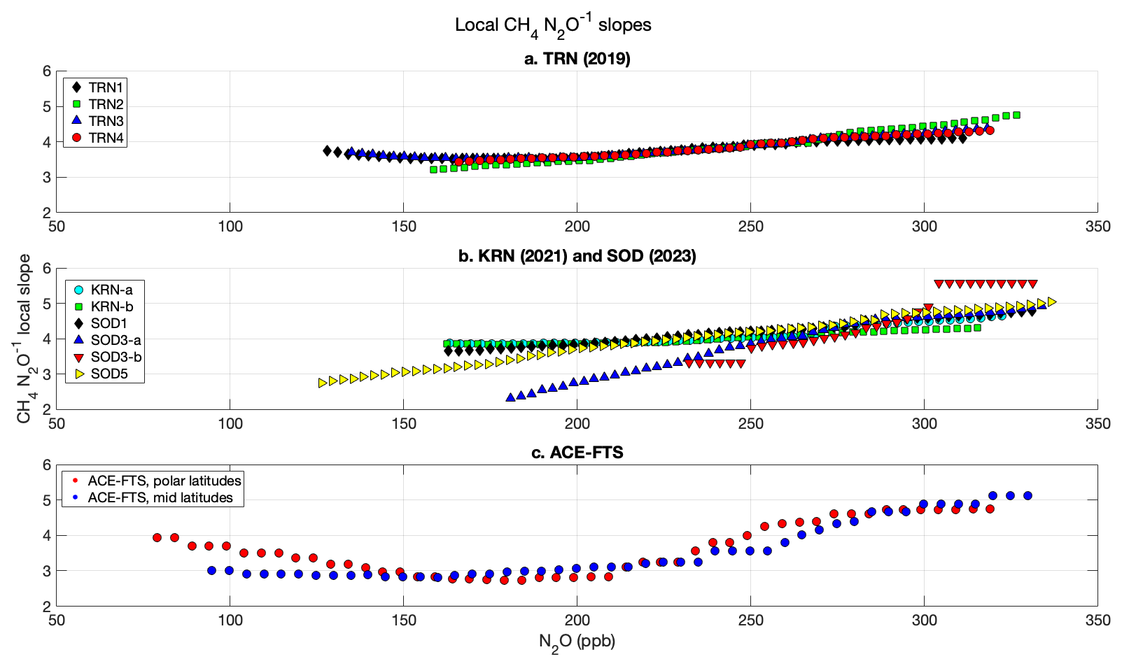
The method adopted to infer the local tracer-tracer slopes follows the approximations of previous studies (Brown et al., 2013; Laube et al., 2013; Leedham Elvidge et al., 2018; Volk et al., 1997). The correlation slopes between COS (or CH₄) and N₂O were calculated every 3 ppb of N₂O, over N₂O ranges of 100 ppb. The N₂O range width was chosen to prevent biases due to, for example, annual cycles or other short-term processes that may cause deviations in the slope curvatures (Volk et al., 1997). The inferred local slopes against N₂O (used as a proxy for altitude mapping) are shown in Fig. 4a–c for COS, and in Fig. 5a–c for CH₄. The clearly atypical behavior of TRN4, KRN-a and SOD3-b will be presented and discussed in Sect. 3.2.3. The lowermost slopes (N₂O > 300 ppb) were excluded from the slope analysis to prevent biases due to tropospheric air fluxes – which are not constant unless species are in steady state (Brown et al., 2013; Volk et al., 1997) – while the highest side of the profiles (N₂O < 200 ppb) were excluded due to non-uniform deviations from the expected curves (Volk et al., 1997). The uncertainties at the tropopause were inferred applying the bootstrap method (Laube et al., 2013; Leedham Elvidge et al., 2018; Volk et al., 1997) within the 200–300 ppb N₂O range.

Figure 4 Local COS N₂O⁻¹ slopes (ppt ppb⁻¹) obtained from AirCore and ACE-FTS profiles.

Figure 5 Local CH₄N₂O⁻¹ slopes (ppb ppb⁻¹) from obtained AirCore and ACE-FTS profiles.

3.2.3 Data deficiency and flagging of outliers

Figures 4–5 show the local slopes against N₂O for both COS and CH₄ obtained from data collected during sampling campaigns and from ACE-FTS data. Consistently to what was observed with the Plumb and Ko (1992) method, KRN-a, KRN-b and SOD3-b show clearly different behaviours when compared to the other profiles. As discussed previously, the measured KRN-a profiles showed significantly lower COS mole fractions between 17–20 km altitude, approximately corresponding to the selected N₂O range. This feature is also reflected in the estimated local slopes, which were therefore considered an outlier. KRN-b slopes are affected by missing data in the lower stratospheric section of the profile (roughly between 10.5–13.5 km). SOD3-b, instead, was refined due to observed contaminations–the restricted data range and the data gaps over the profile determined caused the local slopes to be significantly different from the ones of other flights, and therefore were considered not reliable. A similar issue is noticeable for the COS local slopes of TRN4. For this flight, clear signs of COS contaminations were identified between 9.3–13.9 km. These signs were not noticeable among the other measured tracers. The missing COS data determined the local linear regressions to be performed over less data points and to be biased by the highest and lowest sides of the COS profiles, determining the downwards trend for N₂O > 250 ppb (Fig. 4). Clear deviations from the main trends are clearly noticeable for SOD3-a and SOD3-b in the CH₄-N₂O local slopes, as well.

3.3 N₂O lifetime

The N₂O stratospheric lifetime is relatively well-known and has been estimated from reaction rates derived from vertical profiles of O₃ and temperature (Prather et al., 2015). Krysztofiak et al. (2015) adopted a lifetime of 117 ± 20 years (NOAA, 2003). Karu et al. (2023) used a $T_{{\mathrm{N}}_{\mathrm{2}}\mathrm{O}}$ of 116 ± 9 years, following the estimate of Prather et al. (2015). However, the N₂O lifetime has been reported to decrease consistently at a rate of −2.1 ± 1.2 % per decade between 2005 and 2021 (Prather et al., 2023). Moreover, the N₂O lifetime has been reported to depend on solar activity, which causes a variability of approximately 7 % (Prather et al., 2015). Eventually, we chose to infer N₂O lifetime in 2019, 2021 and 2023 from the 116 ± 9 years estimate (Prather et al., 2015), given the small −2.1 ± 1.2 % per decade decreasing trend (Prather et al., 2023) is not significant over such a short time span and that any variability due to solar activity lies within the reported uncertainty.

4 Results

We estimated the stratospheric lifetimes of COS and CH₄, along with their respective sinks, based on the tropospheric burdens of COS, CH₄ and N₂O and the slopes derived from stratospheric COS-N₂O and CH₄-N₂O correlations.

4.1 Atmospheric burdens

Burdens represent the atmospheric mass of a specific tracer, obtained multiplying its mole fraction by the total atmospheric mass (roughly 5.15 × 10²¹ g). However, since the application of burdens in the given lifetime formulas requires a ratio of two tracers, the total atmospheric mass factor would be cancelled out. Therefore, we report the burdens as mean atmospheric mole fractions. COS tropospheric burdens estimated following Andrews et al. (2001) (Sect. 3.1.1) decreased from 490 ± 18 ppt in 2019 to 479 ± 21 ppt in 2021 and then increased again to 487 ± 18 ppt in 2023. Although not significant, this trend differs from the constant and significant increase of N₂O (from 332.0 ± 0.7 ppb in 2019 to 336.8 ± 2.0 ppb in 2023) and CH₄ (from 1844.6 ± 9.9 ppb in 2019 to 1899.2 ± 9.9 ppb in 2023). These burdens were applied in the Plumb and Ko (1992) method. The total atmospheric global burdens of COS, N₂O and CH₄ were also estimated to be implemented in the Volk et al. (1997) method. The total COS atmospheric burden decreases from 468 ± 9 ppt in 2019 to 457 ± 9 ppt in 2023. The total atmospheric burden of N₂O increases from 322.3 ± 2.5 ppb in 2019 to 324.0 ± 3.6 ppb in 2023, while CH₄ shows an increase from 1806.6 ± 14.1 ppb in 2019 to 1845.9 ± 20.5 ppb in 2023. These trends, reasonably, resemble the general tropospheric trends but are reduced by the weighted average with the stratospheric mole fractions.

4.2 COS

4.2.1 COS-N₂O stratospheric correlations

The correlation slopes between COS and N₂O (Table S3) will be expressed as $\mathrm{d}{\mathit{\sigma }}_{{\mathrm{N}}_{\mathrm{2}}\mathrm{O}}\mathrm{d}{\mathit{\sigma }}_{\mathrm{COS}}^{-\mathrm{1}}$ (ppb ppt⁻¹), as these are the values that are implemented in Eq. (2), with the N₂O mole fraction expressed in ppb and COS mole fraction in ppt. At mid latitudes, we find an average slope of 0.431 ± 0.029 (ranging between 0.405 and 0.463 ppb ppt⁻¹). At polar latitudes, the average slope is 0.470 ± 0.048. Noticeably, SOD1 has a significantly steeper slope than the other flights. The ACE-FTS averaged profiles return a slope of 0.436 ± 0.003 ppb ppt⁻¹ at mid latitudes and 0.456 ± 0.004 ppb ppt⁻¹ at polar latitudes, with the low uncertainties likely ascribable to the averaging over numerous singular profiles. In both AirCore and ACE-FTS profiles the slopes at polar latitudes are generally steeper than the ones at mid latitudes.

The slopes at the tropopause (Table S4) result in averages of 0.438 ± 0.046 ppb ppt⁻¹ at mid latitudes and of 0.482 ± 0.031 ppb ppt⁻¹ at polar latitudes. The corresponding ACE-FTS slopes are 0.429 ± 0.008 ppb ppt⁻¹ at mid latitudes and 0.483 ± 0.007 ppb ppt⁻¹ at polar latitudes. These $\mathrm{d}{\mathit{\sigma }}_{{\mathrm{N}}_{\mathrm{2}}\mathrm{O}}\mathrm{d}{\mathit{\sigma }}_{\mathrm{COS}}^{-\mathrm{1}}$ correlation slopes extrapolated at the tropopause result to be steeper at higher latitudes, similarly to what was observed with the Plumb and Ko (1992) method.

4.2.2 COS stratospheric lifetime and sink estimates

The stratospheric lifetime of a tracer is unique, although its estimates may result in slight differences, depending e.g. on latitude (Krysztofiak et al., 2015). Therefore, in the following paragraphs lifetime estimates from AirCore profiles and ACE-FTS averaged profiles will be reported separately for mid and polar latitudes. The stratospheric COS lifetime calculated following Plumb and Ko (1992) range between 69–90 years, with an overall average (for latitudes > 47° N) of 76 ± 6 years, corresponding to an average stratospheric sink of 37 ± 3 GgS yr⁻¹, ranging between 31–41 GgS yr⁻¹. The average lifetime derived from mid-latitude data in 2019 is 74 ± 5 years, while the average lifetime inferred from profiles collected at polar latitudes between 2021 and 2023 is 79 ± 9 years. Although the lifetime estimates from the most recent polar campaigns seem to be slightly longer than the ones obtained previously at mid-latitude, the difference between the two is not significant. No significant difference was found between stratospheric COS lifetime calculated from ACE-FTS observations and AirCore profiles.

Following the methodology described in Volk et al. (1997), COS lifetime falls in a range of 71–83 years, averaging at 78 ± 7 years over the lifetime estimates retrieved from AirCore data, corresponding to an average sink of 35 ± 3 GgS yr⁻¹ (ranging from 32 to 39 GgS yr⁻¹). The average lifetime derived from mid-latitude profiles is 74 ± 8 years, while the lifetime estimations derived from profiles measured at polar latitudes is 79 ± 5 years. Compared to the results obtained with the method of Plumb and Ko (1992), these lifetime estimates are not significantly different. This method, too, resulted in coherent lifetime estimates between ACE-FTS and AirCore profiles. A comparison between the lifetime obtained with the two different method is presented in Fig. 6. The lifetime estimates do not differ significantly between the two methods.

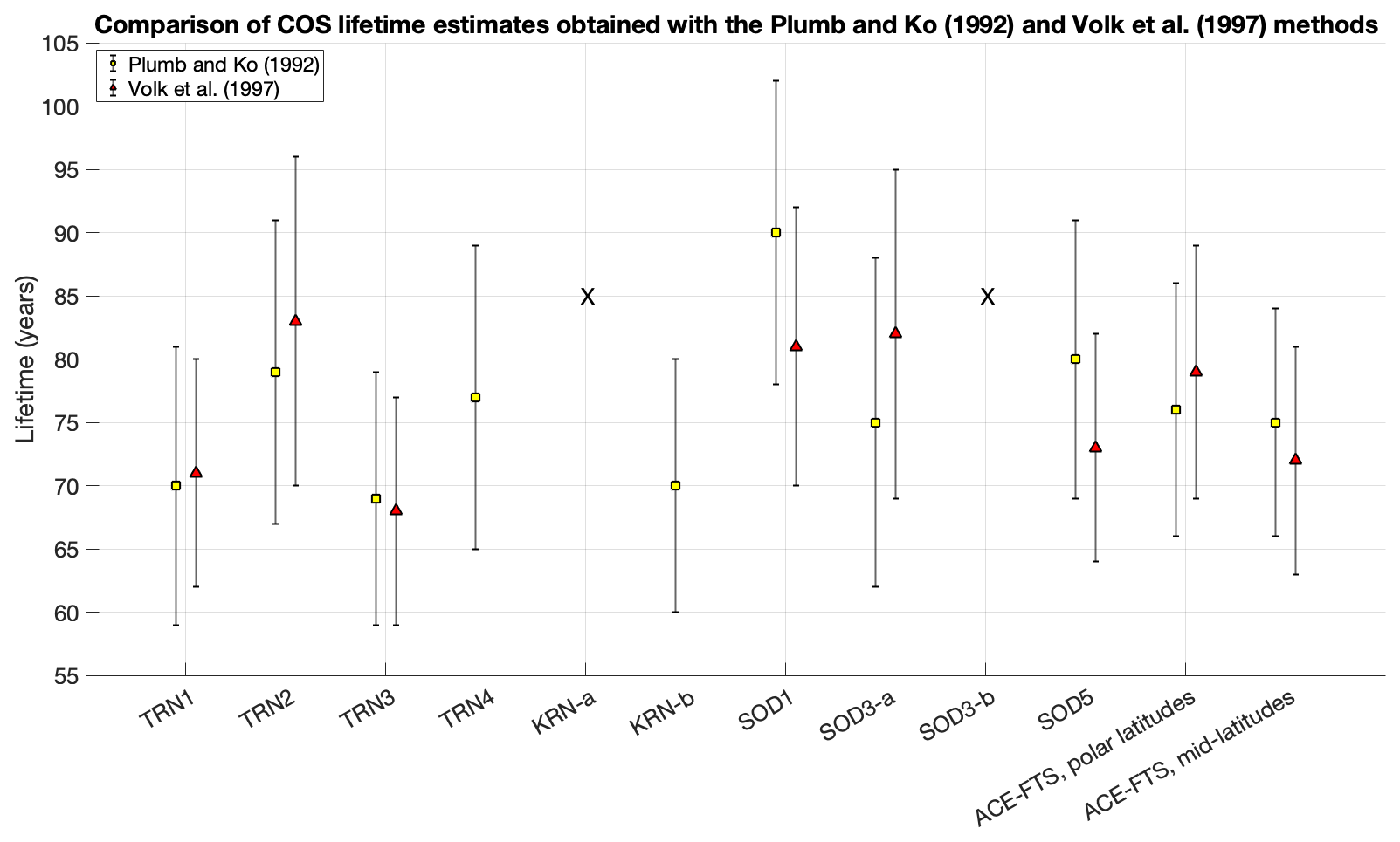
Figure 6 Calculated COS lifetime for AirCore samples and ACE-FTS observations obtained following the two methodologies. Datasets for which it was not possible to apply any of the two methods reliably are marked by an “X”.

4.3 CH₄

4.3.1 CH₄-N₂O correlations

Similarly to COS, the slopes between CH₄ and N₂O will be expressed as $\mathrm{d}{\mathit{\sigma }}_{{\mathrm{N}}_{\mathrm{2}}\mathrm{O}}\mathrm{d}{\mathit{\sigma }}_{{\mathrm{CH}}_{\mathrm{4}}}^{-\mathrm{1}}$ in ppb ppb⁻¹ (Table S6). In all cases, the R² values confirm a very tight relationship between the two tracers. The application of the Plumb and Ko (1992) method leads to an average slope at mid latitudes of 0.2537 ± 0.0022, while at polar latitudes it is 0.2381 ± 0.0063. Interestingly, it is also possible to notice lower slopes for the SOD profiles when compared to the KRN ones. ACE-FTS averaged profiles result in a slope of 0.2217 ± 0.0053 at polar latitudes and 0.2647 ± 0.0118 at mid latitudes, in both cases slightly higher than the ones estimated from the AirCore profiles. Both slopes inferred from ACE-FTS and AirCore profiles are steeper at mid latitudes than at polar latitudes.

The application of the Volk et al. (1997) method resulted in $\mathrm{d}{\mathit{\sigma }}_{{\mathrm{N}}_{\mathrm{2}}\mathrm{O}}\mathrm{d}{\mathit{\sigma }}_{{\mathrm{CH}}_{\mathrm{4}}}^{-\mathrm{1}}$ slopes at the tropopause (Table S8) ranging between 0.2374–0.2473 at mid latitudes (with an average of 0.2416 ± 0.0043) and between 0.2361–0.2552 at polar latitudes (with an average of 0.2376 ± 0.0092). This resembles the latitudinal trends obtained with the Plumb and Ko (1992) method. However, the differences between mid and polar latitudes in this case are not significant. The slopes at the tropopause obtained from the ACE-FTS datasets are 0.2343 ± 0.0169 at mid latitudes and 0.1948 ± 0.0098 at polar latitudes, resulting again in slightly steeper slopes at mid latitudes than at polar latitudes.

4.3.2 CH₄ stratospheric lifetime and sink estimates

The stratospheric CH₄ lifetime range resulting from AirCore data with the Plumb and Ko (1992) method (Table S7) spans between 153–166 years. The lifetime estimates resulting from data collected at polar latitudes appear to be slightly shorter than the ones obtained from mid latitude observations, although the difference is not statistically significant. The consequent stratospheric sink falls within the 24–27 TgC yr⁻¹. This trend is resembled by the lifetime estimates obtained following the method of Volk et al. (1997), which yields CH₄ stratospheric lifetime estimates ranging between 149–162 years, with the shortest lifetime results obtained from datasets collected at polar latitudes. The associated stratospheric sink is 24–26 TgC yr⁻¹. A comparison between the results from both methods is presented in Fig. 7. CH₄ lifetime estimates obtained with the Volk et al. (1997) method are generally shorter, although not significantly, than the ones obtained following Plumb and Ko (1992) with the biggest differences observed between the results obtained with the ACE-FTS datasets. All results will be further discussed in Sect. 5.

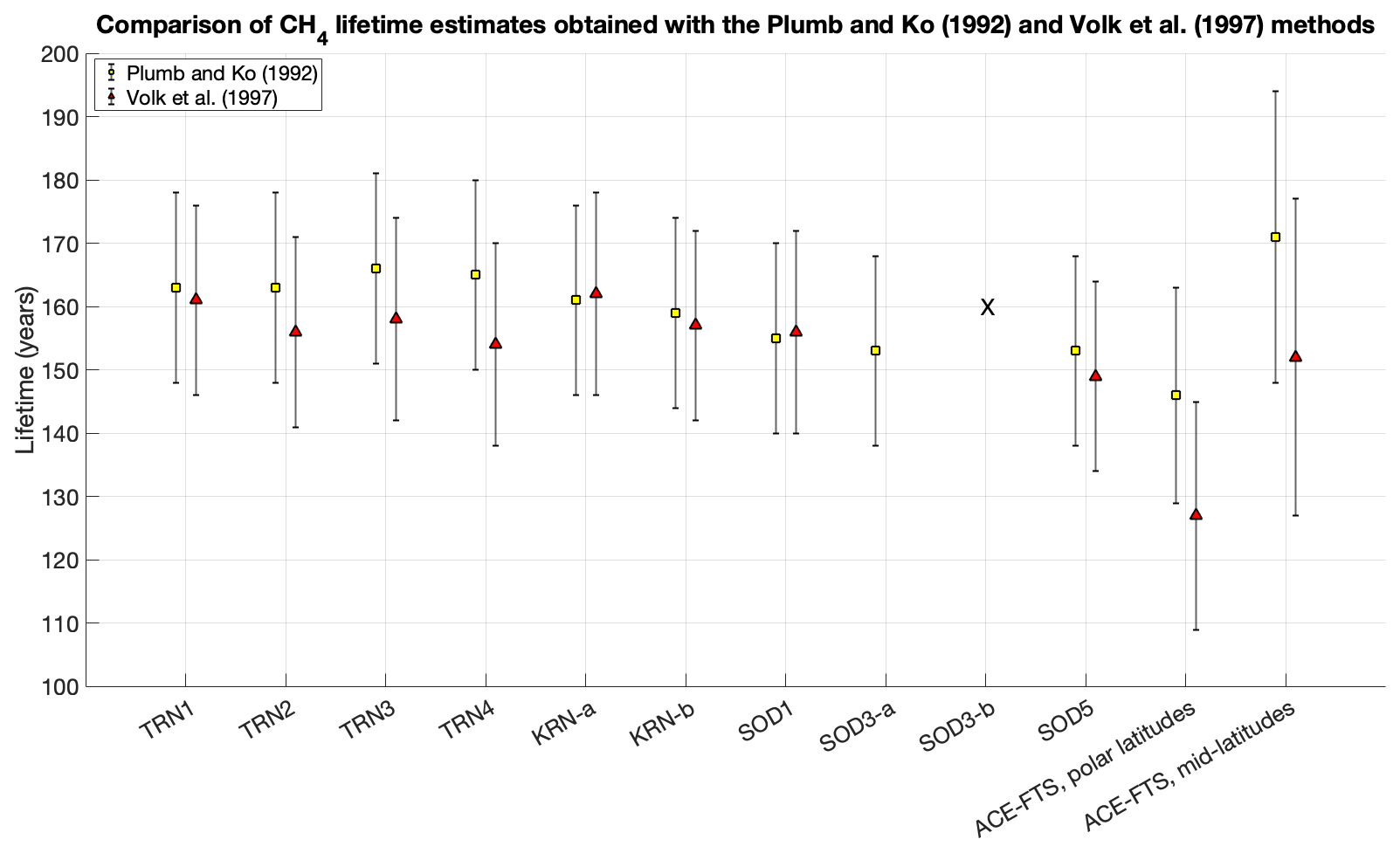
Figure 7 Calculated CH₄ lifetime for AirCore samples and ACE-FTS observations obtained following the methods of Plumb and Ko (1992) and Volk et al. (1997). The missing estimates for SOD3-b are marked as an “X”.

5 Discussion

In the following sections, we compare our results with previous studies regarding COS and CH₄ sources and sinks. For this study, we chose N₂O as the reference gas species with a well-constrained lifetime when applying Eqs. (1) and (2), following the approach of Plumb and Ko (1992) and Volk et al. (1997). The first approach aligns with most recent studies regarding COS lifetime estimations (Karu et al., 2023; Krysztofiak et al., 2015). However, the method of Plumb and Ko (1992) is derived from an idealized global mixing model, with tracers in steady state with negligible local sources or sinks. The method of Volk et al. (1997), later refined by Brown et al. (2013), is more comprehensive and formally accurate, accounting for non-diffusive fluxes across the boundary of the tropics and mid-latitudes in each hemisphere. However, the equation of Plumb and Ko (1992) holds at the extratropical tropopause if the tracers are in slope equilibrium (e.g., their horizontal mixing is much faster than the vertical advection and chemical transformation) and if the difference of the extratropical correlation slopes is small between the two hemispheres (Volk et al., 1997). The tracers considered in this study are all long lived and should respect the slope equilibrium requisite. However, the higher (anthropogenic) surface emissions in the Northern Hemisphere for N­₂O and CH₄ can influence the stratospheric air composition and disrupt the slope equilibrium, in particular in the lowermost stratosphere, which may undermine the application of the Plumb and Ko (1992) method. For example, the relatively faster increase in atmospheric CH₄ compared to N₂O can cause the tracer-tracer relationship to curve in the lowermost part of the stratospheric correlation. This may also happen due to seasonal cycles. COS long-term trends are generally less pronounced, but its photosynthesis-driven seasonal cycle is stronger in the Northern Hemisphere than in the Southern Hemisphere (Remaud et al., 2023). However, the lifetime estimates obtained in this study for both COS and CH₄ are not significantly different between the two methods (Figs. 6, 7). The tracer-tracer correlation slopes retrieved for the Plumb and Ko (1992) method were calculated over specific ranges for both COS and CH₄, to prevent biases due to the slope curvatures near the tropopause and in the higher parts of the profiles (Figs. 2 and 3). Therefore, the results suggest that the local tracer-tracer correlations in the N₂O range between roughly 200 and 300 ppb may respect the conditions for the application of the Plumb and Ko (1992) method. The apparent COS and CH₄ lifetimes obtained with the Plumb and Ko (1992) and with the Volk et al. (1997) methods do not differ significantly (see Sect. 4.2.2 and 4.3.2).

It should be noted that different studies applied different approaches to obtain lifetime estimates. Earlier studies applied the Plumb and Ko (1992) method, often using CFC-12 instead of N₂O as the reference tracer (Barkley et al., 2008; Engel and Schmidt, 1994). While this study presents data obtained by continuous sampling followed by mid-IR spectrometry analysis in a controlled laboratory environment, previous studies used different methodologies to obtain mole fractions of tracers. Engel and Schmidt (1994) collected discrete whole-air samples with a cryogenic sampler. Barkley et al. (2008) used observations obtained from solar occultation measurements from ACE-FTS in 2004–2006. Krysztofiak et al. (2015) obtained their data from the SPIRALE balloon-borne spectrometer. The results of Toon (1991) were reported by Krysztofiak et al. (2015) and they were obtained from the Jet Propulsion Laboratory (JPL) MkIV FTIR ground-based spectrometers observations. Karu et al. (2023) collected and analyzed whole-air samples in the upper troposphere/lowermost stratosphere (UT/LMS, 10–12 km).

Karu et al. (2023) presented another discrepancy in the methodologies followed to estimate the stratospheric lifetime of the tracers: the altitudinal range covered by the observations. Our profiles cover altitudes between roughly 15 and 22 km, comparable with highest altitudes observed by Krysztofiak et al. (2015) and Barkley et al. (2008). While Toon (1991) and Toon et al. (2018) measured COS vertical profiles up to 40 km, Karu et al. (2023)'s observations were limited to observations between 10 and 12 km altitude. At such low altitudes, the mixing of lower stratospheric with tropospheric air is very likely to bias the tracer-tracer correlations and the consequent lifetime estimates.

As stated in Sect. 3.1.1, another noticeable methodological difference concerns the estimation of the tropospheric burden of the tracers. Since the tropospheric burden directly affects the calculation of a tracer's sink, this may be a major cause of discrepancies for such estimates, as will be discussed in the following sections.

5.1 COS stratospheric lifetime and sink

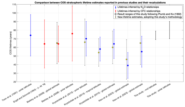
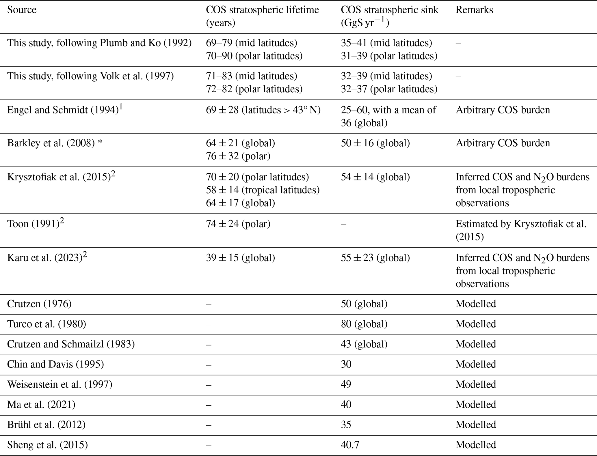
Figure 8 shows the results of previous studies that estimated COS stratospheric lifetime, which are also summarized in Table 2 together with the available sink estimates. These studies estimated the stratospheric sink of COS from modelling or observational efforts, with estimates ranging between 30–80 GgS yr⁻¹ (Brühl et al., 2012; Chin and Davis, 1995; Crutzen, 1976; Crutzen and Schmailzl, 1983; Ma et al., 2021; Sheng et al., 2015; Turco et al., 1980; Weisenstein et al., 1997). Following the method of Plumb and Ko (1992) and Volk et al. (1997) our COS lifetime estimates at mid latitudes (Sect. 3.2.2, Table S5) are not significantly different from each other (Fig. 6) and fall in a range somewhat higher, although not significantly, than previous global estimates (Barkley et al., 2008; Engel and Schmidt, 1994; Krysztofiak et al., 2015). Coherently with literature, we found slightly longer lifetime estimates from profiles collected at higher latitudes (Sect. 4.2.2, Table S5). Previous COS lifetime estimates obtained from polar latitude observations fall in a 70–76 years range (Barkley et al., 2008; Krysztofiak et al., 2015; Toon, 1991) and are not significantly different from our results (Fig. 8, Table 2).

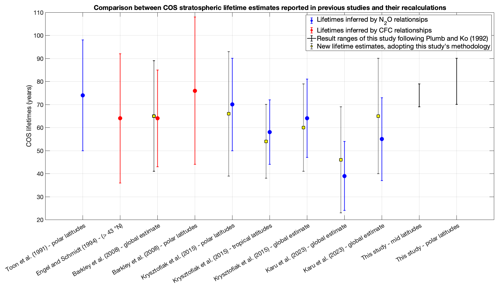
Figure 8 Comparison between COS lifetime estimates of previous studies with their recalculations with new tropospheric burdens obtained following the methods of this study (based on Andrews et al., 2001), in chronological order. The ranges reported for this study correspond to the Plumb and Ko (1992) method, which was also adopted in the studies presented in this figure.

As reported in Table 2, the stratospheric COS sinks we derived with the Plumb and Ko (1992) and Volk et al. (1997) methods are consistent with each other (Sect. 4.2.2). Although the difference between the two methods is not statistically significant, our results are generally smaller than most results from previous studies (30–80 GgS yr⁻¹, see Table 2). One exception is represented by Chin and Davis (1995), who estimated the stratospheric COS sink to be 30 GgS yr⁻¹. As mentioned in Sect. 3.1.1, all studies followed different approaches to define the tropospheric burden of COS. Since the sink is simply derived by the ratio between burden and lifetime, this has surely influenced the final result for each study. Additionally, a decreasing tropospheric burden is found for COS between 2015–2021, confirmed by recent observations (Belviso et al., 2022; Gurganus et al., 2026; Hannigan et al., 2022). A decrease has been also observed in the stratospheric abundance of COS since 2016 (Gurganus et al., 2026). Although the COS tropospheric burden seems to be increasing again in the more recent years, the N₂O tropospheric abundance has always been rising steadily. The opposed trends, of course, reciprocally affect the burdens' ratio in Eq. (2) leading to smaller estimates of the COS stratospheric sink for a given slope value. Furthermore, small differences can be found also in the N₂O COS⁻¹ slope within each campaign (Table S3). As explained in Zanchetta et al. (2026) and explained further in Sect. 5.3, we speculate that daily atmospheric variability and/or interactions of COS or sampling equipment with other tracers may also cause biases in each flight, which may therefore increase the variability in the results. Another potential bias may be caused by uncertainties in altitude mapping of AirCore profiles (Karion et al., 2010; Membrive et al., 2017; Tans, 2022; Wagenhäuser et al., 2021). However, it was not possible to define the cause of these differences confidently with the available data. Overall, finding non-significant differences for neither lifetime nor sink estimates within our campaigns and with existing literature suggests no significant decreasing or increasing trends in the stratospheric sink of COS.

Table 2 Calculated COS lifetime and sink estimates compared with the ones reported by previous studies. The studies marked with ¹ inferred COS lifetime from a CFC-12-COS correlation. The studies marked with ², similarly to this one, inferred COS lifetime from a N₂O-COS correlation. The reference to Toon (1991) indicates the results from JPL MkIV interferometer previously reported by Krysztofiak et al. (2015) and is meant to acknowledge the source of the data.

5.1.1 Sensitivity of results to different methodologies

All the COS-N₂O slopes presented in this study are generally lower than the ones calculated by Krysztofiak et al. (2015) and Karu et al. (2023). This is most likely due to the different altitude ranges where the regressions are performed, together with day-to-day variability and different observational periods.

As illustrated in Sects. 3.1.1 and 5.1, several studies applied the Plumb and Ko (1992) method to calculate the stratospheric COS lifetime estimating tropospheric mole fractions with different methods, or choosing averaged or even arbitrary values. We tried to re-calculate these estimates, when possible, by correcting the tropospheric mole fractions with values obtained following the method of Andrews et al. (2001) presented in Sect. 3.1.1. Since the available data included tropospheric mole fractions in MLO and SMO for COS (2001–2021) and N₂O (1996–2024), it was possible to re-calculate both tropospheric burdens for the studies who investigated the stratospheric lifetime using the same tracers (Karu et al., 2023; Krysztofiak et al., 2015). Additionally, it was possible to calculate a new COS burden for Barkley et al. (2008). The parameters are listed in Table S9.

In the case of Krysztofiak et al. (2015) and Karu et al. (2023), the slopes of the tracer-tracer regressions were reported and it was possible to recalculate the stratospheric lifetime and sink of COS with new estimates of COS and N₂O tropospheric burdens. It is important to notice that in the case of Karu et al. (2023), due to the limited altitudinal range of the observations, the tracer-tracer regression may have been biased by mixing with tropospheric air, which has probably affected the final lifetime estimates. The newly calculated lifetime results obtained with our method are generally shorter for Krysztofiak et al. (2015), who adopted relatively high tropospheric burdens, and generally higher for Karu et al. (2023), who instead opted for stratospheric mole fractions to infer the burdens of Eq. (1). Karu et al. (2023) expressed the burdens following two different methods to define the tropopause height (following the potential vorticity and thermal definitions), but in both cases based the estimation of the burdens on stratospheric mole fractions. When it comes to sinks estimations, the differences become less marked. This is due to the nature of the calculation, which requires to divide again by the COS burden, reducing the bias related to this parameter. For Barkley et al. (2008) the estimation of the COS burden between 2006 and 2008 (the period of their campaign) is so close to the value they chose arbitrarily that no significant difference was found.

In all cases, the newly calculated lifetime and sink estimates are not significantly different from the original ones. However, the region where the regressions are performed and the estimated tropospheric burdens are critical to infer the lifetime of a tracer using the Plumb and Ko (1992) method. Overall, no clear trend in COS lifetime was observed over time nor using the original estimates of previous studies, nor with the recalculations obtained using our methodology.

5.2 CH₄ stratospheric lifetime and sink

CH₄ stratospheric lifetime and sink were calculated following the same methodology that was used for COS. The resulting CH₄ stratospheric lifetime estimates obtained with the Plumb and Ko (1992) method are consistent with the ones derived using the method of Volk et al. (1997) (Sect. 4.3.2, Tables S7, S8). A generally decreasing trend is observed for CH₄ lifetime estimates from mid to polar latitudes as well as over time. However, similarly to COS, these trends are not statistically significant. Although generally higher when calculated from data collected at polar latitudes and generally lower for mid latitudes observations, CH₄ lifetime estimates from AirCore profiles do not differ significantly from their respective ACE-FTS values. These latter estimates are associated with larger uncertainties with the Volk et al. (1997) method due to larger uncertainties regarding the extrapolated slope at the tropopause for these datasets. This is due to the lower number of datapoints over which the linear regressions are performed, which affects in particular the bootstrapped values at the tropopause retrieved following Volk et al. (1997). Moreover, the slopes at tropopause level inferred from ACE-FTS data show larger differences between different latitudes. We speculate that this may be due to the more formally correct nature of the Volk et al. (1997) method, which can better capture stratospheric transport features. In fact, as will be illustrated in Sect. 5.3, it is possible that the AirCore samples we collected at polar latitudes still reflect mid-latitude air features, while ACE-FTS averages over long periods may be more representative of polar air masses. Nevertheless, the stratospheric lifetime estimates obtained from AirCore profiles agree well with the modelled 152 and 159.6 years global estimate presented in SPARC (2013) Report No. 6 and the 159 ± 35 years inferred by Brown et al. (2013) from ACE-FTS remote sensing observations during the northern hemisphere summer.

The stratospheric sink estimated from our measurements are also consistent regardless on the employed method (Tables S7, S8). Our results are lower than earlier estimates of 34 TgC yr⁻¹ (Hein et al., 1997) and 30 TgC yr⁻¹ (Lelieveld et al., 1998), but fall within the more recent stratospheric loss range of 12–37 TgC yr⁻¹ (Saunois et al., 2020).

Overall, within the methods applied in this study, we believe that COS and CH₄ lifetime and sink calculations share the same sources of uncertainty. The differences between burdens and local tracer-tracer slopes obtained with the two employed methods remained moderate within the selected altitudinal range. Since the two studies are based on a similar mathematical construction, where Volk et al. (1997) is more formally correct these results suggest that Plumb and Ko (1992) provides an acceptable approximation for estimating the lifetime of COS and CH₄ within these altitudes. Concerning CH₄, the increasing burden (Sect. 3.1.1, 3.2.2) is most likely the reason behind the slightly decreasing (although not significant) trend in stratospheric lifetime assessments. In fact, the CH₄ burden increase is relatively faster than the N₂O increase. Some small flight-to-flight variability can be observed in the N₂O CH${}_{\mathrm{4}}^{-\mathrm{1}}$ linear regression slopes, with the slopes at polar latitudes being generally lower than the ones at mid latitudes with both methods (Tables S6, S8). The reason behind this variability remains overall unclear. As previously speculated for COS, we believe this could be due to atmospheric transport features. Nevertheless, the resulting lifetime and sink estimates are statistically consistent with each other as well as with ACE-FTS estimates, and fall well within the ranges reported in the existing literature.

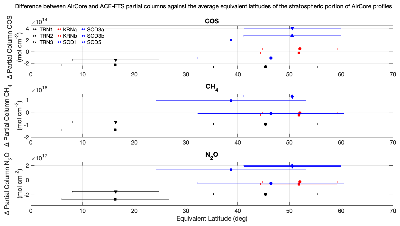
Figure 9 Retrieved differences between stratospheric partial columns of AirCore and ACE-FTS profiles, against the average stratospheric equivalent latitude of AirCore profiles. The partial columns are reported in molecules cm⁻².

5.3 Equivalent Latitude of AirCore observations

To further contextualize the AirCore results and their comparison with ACE-FTS averaged data, the equivalent latitude (Nash et al., 1996) was calculated from the ERA5 hourly potential vorticity data (Hersbach et al., 2023) for every flight. Equivalent latitude, in fact, represents the transport history of air parcels more accurately than geographic latitude, particularly in the upper troposphere/lower stratosphere region. The computed equivalent latitudes for each pressure level of the retrieved AirCore profiles are shown in Sect. S5 (Figs. S20–S28). From these results, we computed the stratospheric partial columns of COS, CH₄ and N₂O for both AirCore profiles and their respective ACE-FTS profiles between the tropopause and 12 km above it, and investigated the difference between them. Figure 9 shows the resulting differences against the average stratospheric equivalent latitude. TRN4 is not shown due to missing data that prevented the calculation of the stratospheric partial column of COS. Overall, it is evident that most of the sampled air had mid-latitude origins and that the partial columns obtained from TRN samples underestimate all tracers when compared to those obtained from ACE-FTS mid-latitude averaged profiles. The opposite is true for the AirCore samples collected in SOD. From the principle of AirCore sampling, we see no reason that biases could differ at the two different sites. Therefore, these opposing differences likely indicate that the AirCore profiles capture localized, latitudinally dependent air masses that are not fully represented by the zonally averaged ACE-FTS. Notably, it is interesting to note that the average equivalent latitude of the samples collected in KRN and SOD is typically well below polar latitudes, which may partially explain the larger discrepancies (though not significant) observed between the CH₄ lifetime estimates obtained with the Volk et al. (1997) method (see Fig. 7).

6 Conclusions

This study derived the mean stratospheric lifetime and sink of COS and CH₄ from continuous AirCore vertical profiles analyzed with a QCLS, using two methods based on the relationship of the two species with N­₂­O in the lower stratosphere. Stratospheric tracer-tracer correlation variability was found among flights, including within the same campaign. This variability may reflect day-to-day changes in stratospheric transport and/or uncertainties associated with sampling and measurement, but the available information does not allow its origin to be fully understood.

Using the method of Plumb and Ko (1992), COS stratospheric lifetime was estimated at 69–79 years at mid latitudes and 70–90 years at polar latitudes, corresponding to sinks of 35–41 GgS yr⁻¹ and 31–39 GgCOS yr⁻¹, respectively. Following the method of Volk et al. (1997), we find consistent results, with COS lifetime estimates of 71–83 years at mid latitudes and 72–82 years at polar latitudes, corresponding to sinks of 32–39 and 32–37 GgS yr⁻¹, respectively. Although these lifetime estimates are generally at the upper end of the range reported in the literature, they are not significantly different from previous values.

For CH₄, the method of Plumb and Ko (1992) yielded stratospheric lifetime ranges between 163­-166 years at mid latitudes and 153–161 years at polar latitudes, while the method of Volk et al. (1997) gave lifetime estimates of 154–161 years (mid latitudes) and 149–162 (polar latitudes), respectively. Considering both methods, these ranges correspond to sink estimates of 24–25 and 24–26 TgC yr⁻¹.

All estimates are consistent with spatially and temporally averaged estimates based on ACE-FTS data, and with literature estimates. Overall, our results show that AirCore measurements can provide robust observational constraints on the stratospheric lifetime and sink of COS and CH₄, provide an additional tool for investigating long-term stratospheric trends, and help refine their representation in atmospheric chemistry and transport models. The results presented in this study suggest that no significant trends in stratospheric removal emerged in recent years for COS and CH₄, regardless of the observed trends for their tropospheric abundances. However, given the reported discrepancies in the methods adopted by previous studies, we advocate for a more standardized methodology for estimating the slopes and tropospheric burdens used to derive the stratospheric lifetime and sink of a tracer with these techniques.