Impact of model resolution and turbulence scheme on the representation of mountain waves and turbulence

Simulating mountain waves and associated turbulence in the upper troposphere and lower stratosphere (UTLS) remains a challenge in numerical weather prediction (NWP). We investigate how the representation of mountain-wave dynamics and turbulence in the ICOsahedral Nonhydrostatic (ICON) model depends on model resolution and turbulence parameterization. ICON simulations were performed in NWP mode (ICON-NWP) with varying horizontal (2, 1 km, 500 m) and vertical (400, 200, 100 m) resolutions, using the operational turbulent kinetic energy scheme (ICON-TKE) and the newly developed two-energy turbulence scheme (ICON-2TE). The simulations were evaluated against high-frequency in situ observations from the Deep Propagating Gravity Wave Experiment (DEEPWAVE) over New Zealand on 12 July 2014, as well as a nested large-eddy simulation (ICON-LES) at 130 m resolution. The results show reasonable agreement with observations: ICON-LES more closely captures wavelength and phase, while ICON-NWP better reproduces wave amplitude. Near-convergence of the primary mountain wave and of turbulence structures requires horizontal grid spacings of 1 km or finer and vertical spacings in the UTLS of 200 m or finer, whereas trapped lee waves and downstream wave structure remain resolution-sensitive at these resolutions. Area-averaged, bulk measures allow this convergence behavior to be characterized more systematically: the low-level gravity-wave momentum flux continues to increase with increasing resolution from 1 km to 500 m. A key finding is that both turbulence schemes yield similar wave structures, despite large differences in simulated turbulent kinetic energy. This discrepancy is attributed to the empirical horizontal-shear source term of the operational TKE-scheme configuration, which produces spurious TKE at km-scale resolution. These results provide guidance on the resolution and turbulence representation needed for reliable simulations of small-scale mountain waves and turbulence in the UTLS.

1 Introduction

The upper troposphere and lower stratosphere (UTLS), spanning roughly 6 to 25 km altitude (Riese et al., 2012), plays a central role in climate dynamics by regulating the distribution of greenhouse gases. As a transition zone between the relatively well-mixed troposphere and the stably stratified lower stratosphere, the UTLS facilitates tracer transport through a range of dynamical processes operating across multiple spatial and temporal scales (Scherllin-Pirscher et al., 2021; Riese et al., 2012). These processes include the large-scale Brewer–Dobson circulation (months to years), Rossby wave breaking and baroclinic cyclones (several days), deep convection on shorter timescales (Schäfler et al., 2023), and small-scale turbulence. Turbulence in the UTLS is particularly important for stratosphere–troposphere exchange of chemical constituents. Unlike the planetary boundary layer, where turbulence is sustained, turbulence aloft is intermittent and localized, producing short-lived but intense mixing events, especially near the tropopause (Mirza et al., 2024). Acting on horizontal scales of a few hundred meters to several kilometers, UTLS turbulence can significantly influence large-scale circulation patterns (Rogel et al., 2023).

Upper-air turbulence in the UTLS can be broadly categorized by its origin into three types: clear-air turbulence, often associated with jet streams; mountain-wave turbulence (MWT), generated by flow over topography; and convectively induced turbulence, linked to thunderstorms (Kim et al., 2023; Ren and Lynch, 2024). Among these, MWT is of particular importance because it poses substantial challenges for aviation safety, flight planning, and route optimization (Mahalov, 2016). Many long-haul flight routes cross major mountain ranges, where MWT occurs frequently and often with high intensity. Understanding mountain-wave dynamics and their associated turbulence is therefore not only relevant for weather and climate research, but also for operational forecasting and aviation risk management.

Mountain waves are a specific type of gravity wave that arises when stably stratified air is forced to flow over topography, producing oscillations with gravity as the restoring force. As these waves propagate upward, their amplitude increases with decreasing air density. When the intrinsic phase speed of the wave approaches the background wind speed, the wave amplitude reaches a maximum and momentum is transferred to the mean flow. Beyond this point, the wave can become unstable and generate turbulence. This occurs either through catastrophic wave breaking, in which the wave is completely destroyed, or through wave saturation, where energy is dissipated into turbulence that limits further amplitude growth. In the latter case, the wave only partially breaks but still produces localized turbulent mixing. These processes illustrate the close coupling of gravity waves and turbulence, which is central to understanding energy and momentum transfer in the UTLS (Liu et al., 1999; Schneider et al., 2017; Dörnbrack et al., 1995; Sharman et al., 2012; Fritts and Alexander, 2003).

Mountain waves play a major role in atmospheric energetics by transporting energy and momentum away from their source regions. They are typically generated in the troposphere and can propagate both vertically into the stratosphere and horizontally over long distances. The structure and propagation of a mountain wave depend strongly on the size and shape of the underlying topography as well as on the vertical profiles of wind, temperature, and moisture in the flow (Durran, 2015). Orographic gravity waves often dominate the global gravity-wave spectrum, with momentum fluxes several times larger than those of non-orographic waves and concentrated over regions of complex terrain (Holt et al., 2017).

Mountain waves have been investigated extensively through ground-based instruments, in situ aircraft measurements, satellite observations, and dedicated field campaigns (Heale et al., 2022; Grubišić and Lewis, 2004; Grubišić et al., 2008; Bougeault et al., 1993; Kuettner and O'Neill, 1981; Bougeault et al., 2001; Wratt et al., 1996; Fritts et al., 2016; Schäfler et al., 2018; Jackson et al., 2018; Rapp et al., 2021). These studies have identified several “hotspots” of gravity-wave activity, such as regions downstream of major mountain ranges (Heale et al., 2022). Despite this rich observational record, forecasting mountain waves and associated turbulence in numerical weather prediction (NWP) and climate models remains highly challenging. The difficulty arises from the multiscale interactions between waves and turbulence, and from the fact that a large part of the gravity-wave spectrum lies below the typical grid resolution of global models and thus must be parameterized (Plougonven et al., 2020; Achatz et al., 2024; Voelker et al., 2024). Recent advances in computational power have enabled mesoscale nested simulations with horizontal resolutions of about 1 km or finer, offering new opportunities to explicitly resolve small-scale processes while still accounting for the large-scale environment provided by coarser parent domains (Muñoz-Esparza et al., 2020; Rogel et al., 2023).

Large-eddy simulation (LES) and direct numerical simulation (DNS) provide powerful tools for investigating turbulence associated with mountain waves at very high resolution. These approaches can resolve small-scale structures that remain inaccessible to operational NWP models. For example, Bramberger et al. (2020) used a two-dimensional model with 200 m horizontal and 100 m vertical grid spacing to simulate a mountain-wave breaking event over Iceland. Their results demonstrated that the observed turbulence could be attributed directly to breaking mountain waves. Such high-resolution studies highlight the potential of LES and DNS to improve physical understanding of mountain-wave turbulence, while also providing valuable benchmarks for evaluating parameterizations in coarser-resolution models.

Several recent modeling studies have addressed the resolution required to capture mountain-wave dynamics and associated processes with fidelity. Lund et al. (2020) and Fritts et al. (2021) investigated the nonlinear evolution of mountain waves over the southern Andes using simulations at 500 m resolution, revealing the complex dynamics that emerge with increasing wave forcing. Extending this work, Fritts et al. (2022) examined how model resolution affects the representation of mountain waves propagating into the thermosphere. Their results showed that coarser resolutions quickly degrade the ability to simulate key wave dynamics, leading to systematic biases in global models that influence both weather and climate predictions. Through simulations of wintertime flow over the southern Andes at horizontal resolutions ranging from 0.5 to 8 km, they demonstrated that resolutions of about 2 km or finer are necessary to adequately capture mountain-wave responses, particularly in the mesosphere.

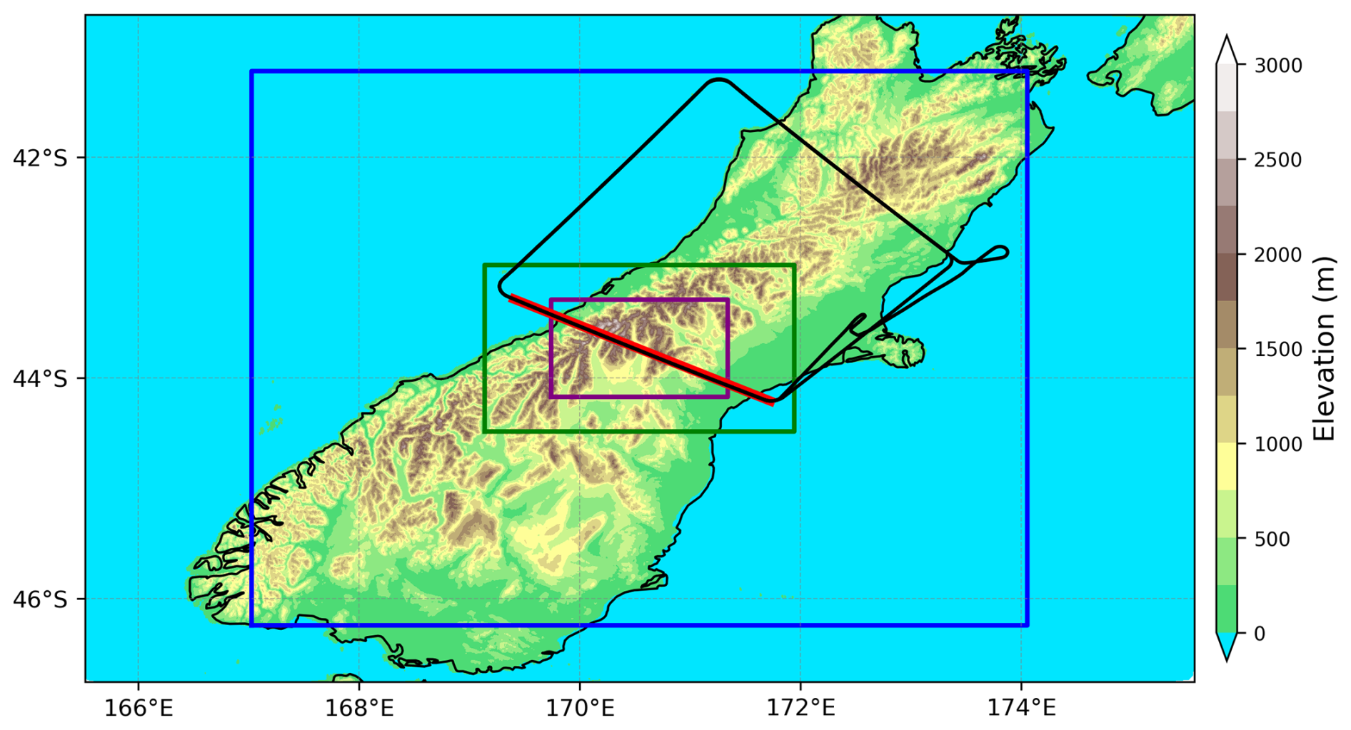
Figure 1 Orography (color shading) and simulation domains for the nested ICON setup: 1 km (full region), 500 m (blue box), and 130 m for the southern flight segment (green box). The red line marks the cross-section along the flight path used for the main analysis, and the purple box indicates the averaging region for calculating bulk properties of the GW field (Sect. 3.4). The black solid line shows the full flight path of research flight FF09 of the Falcon aircraft on 12 July 2014 (17:15–20:15 UTC) during the DEEPWAVE campaign.

Most turbulence parameterizations used in numerical models were originally developed for the atmospheric boundary layer (ABL), but they are not necessarily suited to conditions in the UTLS. The ABL is characterized by a solid lower boundary and strongly influenced by diurnal cycles of radiative heating and cooling, leading to turbulence generation mechanisms that differ fundamentally from those aloft. In contrast, turbulence in the UTLS occurs in a strongly stratified environment, is often patchy and anisotropic, and appears as sudden, localized bursts of velocity and temperature fluctuations that deviate from classical Kolmogorov scaling (Rodriguez Imazio et al., 2023; Kleeorin et al., 2019; Mahalov, 2016; Paoli et al., 2014). The challenges of applying ABL-based schemes at km-scale resolutions in the UTLS have been demonstrated by Muñoz-Esparza et al. (2020), who showed that turbulence parameterization significantly influences gravity-wave activity and vertical mixing in high-resolution weather simulations. Using a case of widespread turbulence over the US Great Plains, they found that a 1 km model tends to overestimate vertical velocities, wave fluxes, and kinetic energy compared to a 250 m LES. These findings underline the need for turbulence parameterizations adapted specifically to UTLS conditions in order to capture wave–turbulence interactions more realistically.

In this study, we evaluate the performance of two turbulence schemes implemented in the ICOsahedral Nonhydrostatic (ICON) limited-area model for simulating mountain waves and associated turbulence in the UTLS. Specifically, we compare the operational turbulent kinetic energy scheme (ICON-TKE) with the newly developed two-energy turbulence scheme (ICON-2TE). Sensitivity experiments are conducted with varying horizontal and vertical resolutions to determine the model configuration required to capture key wave and turbulence characteristics. The simulations are qualitatively evaluated against high-frequency in situ observations from the Deep Propagating Gravity Wave Experiment (DEEPWAVE), a field campaign conducted over New Zealand in 2014, and against a nested large-eddy simulation (ICON-LES) at 130 m resolution. The observational comparison is used primarily to verify that both schemes produce realistic flow structures rather than to provide an exhaustive validation. The remainder of the paper is organized as follows: Sect. 2 describes the ICON model setup, including the two turbulence schemes, the case study, and the analysis methodology. Section 3 presents the evaluation of a reference simulation and the results of the sensitivity experiments, including a discussion of their implications for simulating mountain waves and turbulence in the UTLS. Finally, Sect. 4 summarizes the main findings and provides recommendations for future work.

2 Experimental setup

2.1 Case study and observational data

The case analyzed in this study is a mountain-wave event over New Zealand on 12 July 2014 during the DEEPWAVE campaign, with the topography and study domain shown in Fig. 1. This case is useful because it combines a clearly observed mountain wave with relatively rare high-frequency in situ measurements near the tropopause. Earlier analyses inferred possible signatures of turbulence impacts on tracer distributions in the UTLS region (Lachnitt et al., 2023). Although direct observational evidence of wave breaking was not available, the event provides targeted in situ observations that make it suitable for evaluating how turbulence parameterizations and model resolution affect the simulation of mountain waves in the UTLS.

The synoptic situation during the event was characterized by a trough to the west of New Zealand and a weak low-pressure system to the south of the islands. This configuration produced moderate northwesterly flow across the South Island, i.e., about 10–15 m s⁻¹ at 5 km, oriented perpendicular to the Southern Alps. At tropopause level (around 10 km altitude), winds were also from the northwest, reaching moderate speeds of about 20 m s⁻¹ along the DEEPWAVE flight path. Overall, weak directional shear created favorable conditions for the generation of vertically propagating mountain waves over the South Island.

The DEEPWAVE research flight FF09 was carried out with the DLR Falcon aircraft on 12 July 2014 between 17:15 and 20:15 UTC. The aircraft followed a clockwise rectangular flight track across the South Island to capture the structure of the mountain-wave event (see Fig. 1). To sample vertical variability, the flight pattern consisted of two stacked legs separated by approximately 75 min, with the lower level at 360 hPa (7.9 km) and the upper level at 230 hPa (10.9 km). In the southern segment of the track, the lower leg was flown between 17:30 and 17:50 UTC and the corresponding upper leg between 18:47 and 19:07 UTC. In the northern segment, the lower leg took place from 18:12 to 18:32 UTC and the upper leg from 19:27 to 19:47 UTC. These stacked cross sections provide in situ measurements of mountain waves and turbulence signatures near the tropopause and serve as the observational reference for the model evaluation. Importantly, the simulated primary wave during this period is quasi-stationary, with only weak temporal variations in wave amplitude and vertical structure. The observational comparison therefore focuses on the time of the flight transect, which is representative of the modeled flow regime.

2.2 Model and turbulence schemes

The numerical experiments were performed with the ICOsahedral Nonhydrostatic (ICON) model version icon-2024.01-dwd-2.0, operated in both NWP and LES modes. ICON is a fully compressible atmospheric model jointly developed by the German Weather Service and the Max Planck Institute for Meteorology. It employs an icosahedral-triangular grid constructed using geodesic Delaunay triangulation, a height-based vertical coordinate system, and C-grid staggering (Zängl et al., 2015). The physical parameterizations include the Tiled TERRA land surface scheme (Schulz et al., 2016), a one-moment cloud microphysics scheme with graupel (Seifert, 2008), the low-level flow blocking component of the subgrid-scale orographic drag scheme (Lott and Miller, 1997), and the ecRad radiation scheme (Hogan and Bozzo, 2018).

A central aim of this study is to assess how the simulation of mountain waves and turbulence in ICON depends on both the choice of turbulence parameterization and the model resolution. Two turbulence schemes are considered: the operational turbulent kinetic energy scheme (TKE scheme; Raschendorfer, 2001) and the more recently developed two-energy turbulence scheme (2TE scheme; Bašták Ďurán et al., 2022). The TKE scheme predicts a single turbulent kinetic energy (TKE) and accounts for turbulence generation beyond vertical wind shear through additional empirical source terms for large-scale horizontal shear (HS term) and breaking subgrid-scale mountain waves (SSO term) (Goecke and Machulskaya, 2021). Its development and tuning prioritize operational NWP applications, including aviation turbulence products such as eddy dissipation rate (EDR). In contrast, the 2TE scheme predicts two prognostic turbulence energies, enabling a more flexible representation of anisotropic and stably stratified turbulence. The scheme avoids prescribed minimum diffusion coefficients, dynamically adjusts the turbulence length scale, and employs an assumed probability density function (APDF) method to represent buoyancy production. Through this formulation, the 2TE scheme provides a unified framework for representing turbulence, shallow convection, and subgrid-scale cloud processes (Bašták Ďurán et al., 2018; Singh et al., 2025). Further details on the two turbulence schemes are provided in Appendix A.

While the TKE scheme has long been used operationally and the 2TE scheme is currently under development, their performance in simulating mountain waves and associated turbulence in the UTLS has not been systematically evaluated. A further aim of this study is therefore to provide a first evaluation of the 2TE scheme in this regime, to inform its ongoing development. In addition, the sensitivity of these simulations to horizontal and vertical resolution is not well constrained, despite growing use of km-scale NWP. The case is also demanding in its own right: the Southern Alps of New Zealand present three-dimensional, multi-scale terrain, with several ridges of different heights and orientations, in contrast to the isolated or quasi-two-dimensional ridges of many earlier studies, so that waves from several sources interact. This study therefore investigates how the two turbulence schemes, in combination with different resolutions, represent mountain-wave dynamics, turbulence characteristics, and momentum fluxes during the DEEPWAVE case. The different ICON configurations and sensitivity experiments are introduced in the following subsection.

Table 1 Overview of ICON model experiments used in this study. The table lists the turbulence scheme, horizontal resolution, and grid setup for each configuration, including NWP runs, nested LES, and targeted ICON-TKE sensitivity experiments. SSO refers to subgrid-scale orography, HS refers to horizontal shear, and GP denotes grid points.

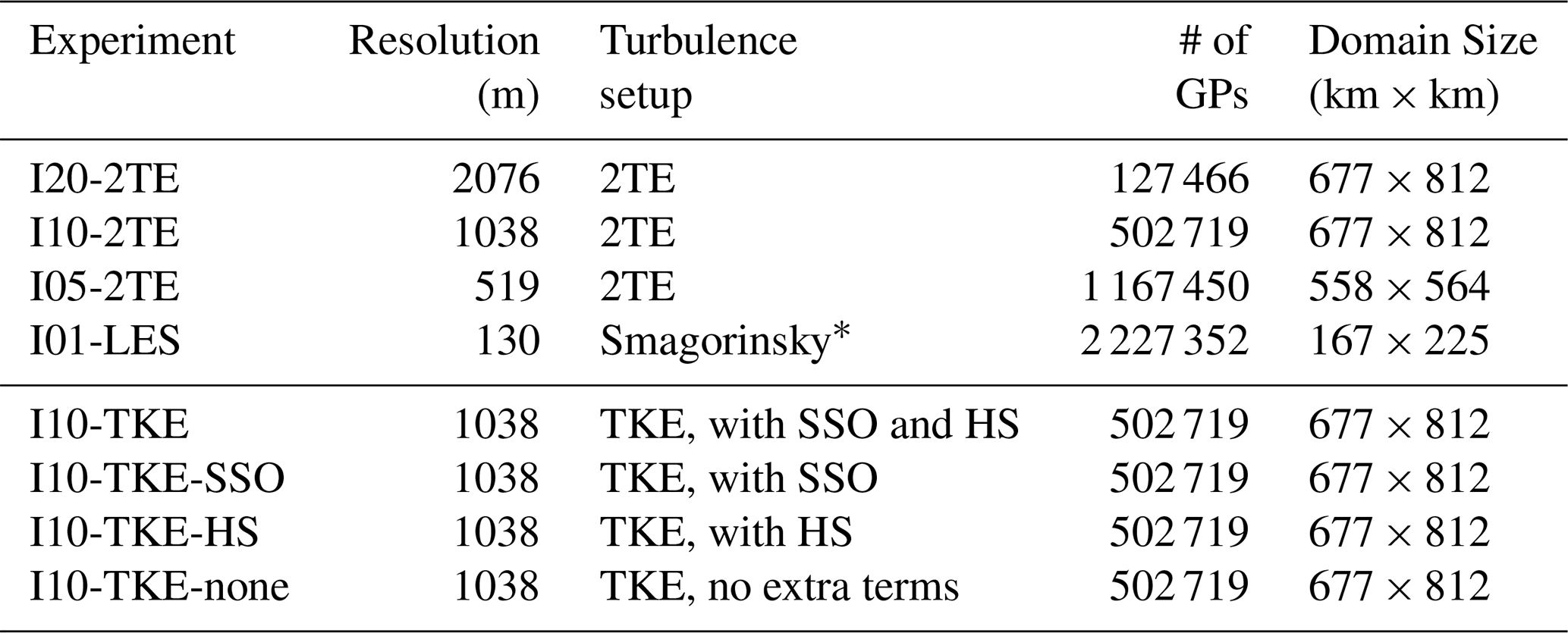
^∗ The LES are run as an online nest consisting of four domains: 1 km, 519 m, 260 m and 130 m.

2.3 Model configurations and simulations

Based on the two turbulence schemes described above, we carried out a set of numerical experiments with varying horizontal and vertical resolutions, complemented by a nested LES and targeted sensitivity runs. The experiments are summarized in Table 1. Limited-area ICON simulations in NWP mode were conducted at horizontal grid spacings of approximately 2 km (I20-2TE), 1 km (I10-2TE, I10-TKE), and 0.5 km (I05-2TE). All configurations employed 137 vertical levels with spacing increasing from about 20 m near the surface and not exceeding 200 m up to 14 km, a model top at 30 km, and Rayleigh damping above 20 km. The simulations were initialized from IFS analyses at 00:00 UTC on 12 July 2014 and integrated for 24 h, with outputs every 30 min and every 5 min between 17:00 and 20:00 UTC. Among these, the I10-2TE simulation was selected as the reference case for the analysis.

An online nested LES configuration at 130 m (I01-LES) targeted the southern flight segment. The LES was realized with four nested domains down to 130 m, with the outermost nest run using the 2TE scheme and the inner nests employing a Smagorinsky closure. To isolate parameterized sources of turbulence production in the TKE scheme, we additionally performed targeted sensitivity runs at 1 km resolution: one with only subgrid-scale orography activated (I10-TKE-SSO), one with only horizontal-shear production activated (I10-TKE-HS), and one with both terms deactivated (I10-TKE-none).

2.4 Bulk characteristics of the GW field

In addition to local characteristics, we also evaluate bulk characteristics of the simulated gravity wave (GW) field over the Southern Alps, namely the area-averaged vertical fluxes of momentum induced by the waves. For this purpose, the model output on terrain-following levels was interpolated to geometric height levels, and averages were taken over the analysis domain shown in Fig. 1. The vertical fluxes of horizontal momentum are defined as

$$\begin{array}{}\text{(1)}& \stackrel{\mathrm{‾}}{\mathit{\rho }{u}^{\prime }{w}^{\prime }}=\stackrel{\mathrm{‾}}{\mathit{\rho }(u-\stackrel{\mathrm{‾}}{u})(w-\stackrel{\mathrm{‾}}{w})},\stackrel{\mathrm{‾}}{\mathit{\rho }{v}^{\prime }{w}^{\prime }}=\stackrel{\mathrm{‾}}{\mathit{\rho }(v-\stackrel{\mathrm{‾}}{v})(w-\stackrel{\mathrm{‾}}{w})},\end{array}$$

where overbars denote horizontal means at a given altitude and primes the corresponding perturbations. The total flux magnitude is then given by

$$\begin{array}{}\text{(2)}& \mathit{\tau }=\sqrt{(\stackrel{\mathrm{‾}}{\mathit{\rho }{u}^{\prime }{w}^{\prime }}{)}^{\mathrm{2}}+(\stackrel{\mathrm{‾}}{\mathit{\rho }{v}^{\prime }{w}^{\prime }}{)}^{\mathrm{2}}}.\end{array}$$

The variance of vertical velocity, $\stackrel{\mathrm{‾}}{w^{\prime \mathrm{2}}}$, follows as a special case of these definitions. Along with the subgrid-scale TKE, these diagnostics characterize the bulk properties of the GW field and parameterized turbulence across different resolutions and turbulence schemes. In particular, area-averaged momentum fluxes provide a measure of convergence with resolution and are an important target quantity for parameterizations in coarse-resolution models.

3 Results and Discussion

We first examine the I10-2TE simulation to establish the baseline characteristics of the wave event. This case serves as the reference for assessing the impact of resolution and turbulence parameterizations in the subsequent subsections. We chose I10-2TE as the reference because, as will be shown, the standard TKE configuration produces excessive and likely unrealistic TKE, making it less consistent as a baseline.

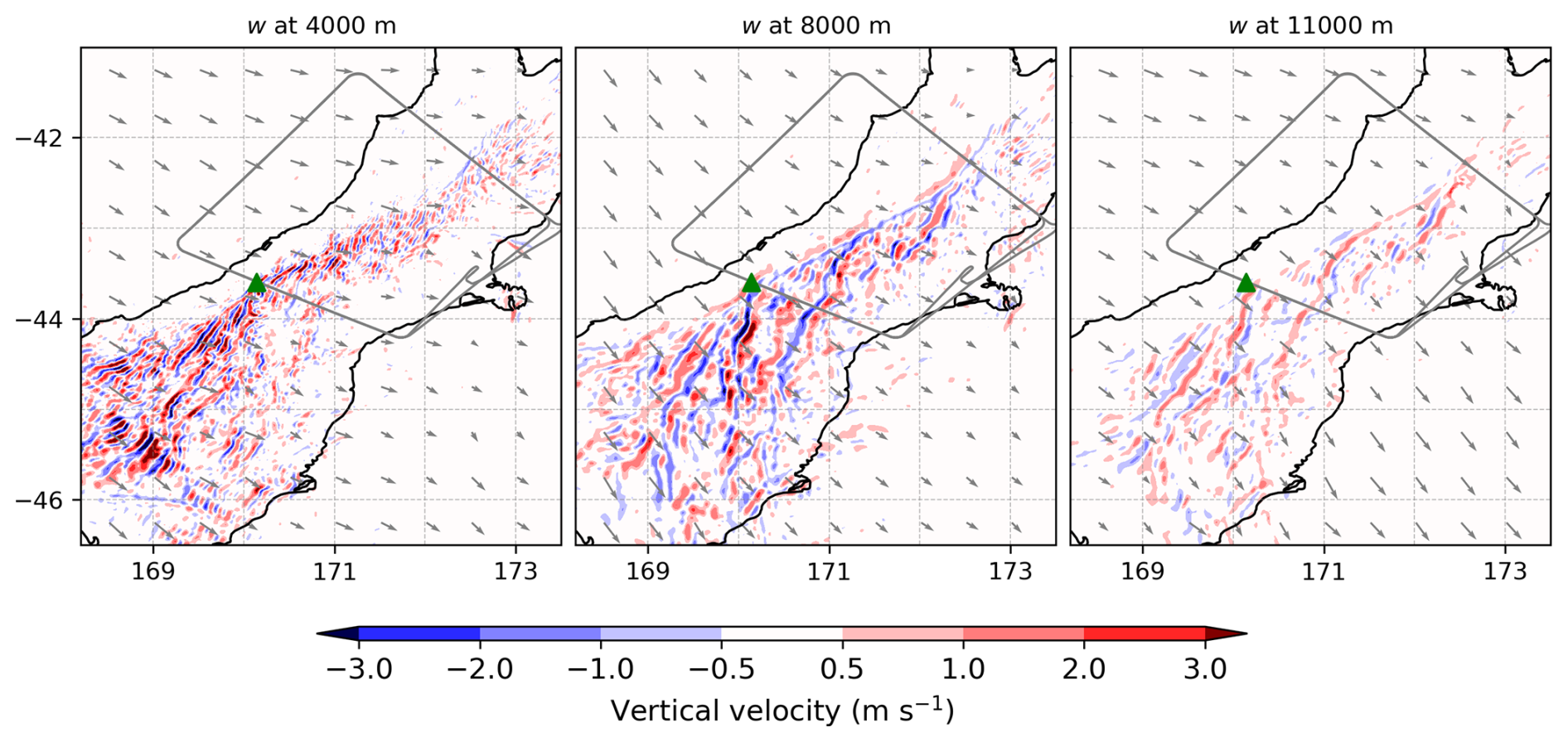
Figure 2 Horizontal cross-sections of vertical wind at three heights, with the upper two corresponding to the lower and upper flight legs, from the I10-2TE simulation at 18:00 UTC on 12 July 2014. Horizontal wind vectors are overlaid. The full flight track is shown by the grey line, and the green marker denotes the location of Mount Cook, New Zealand.

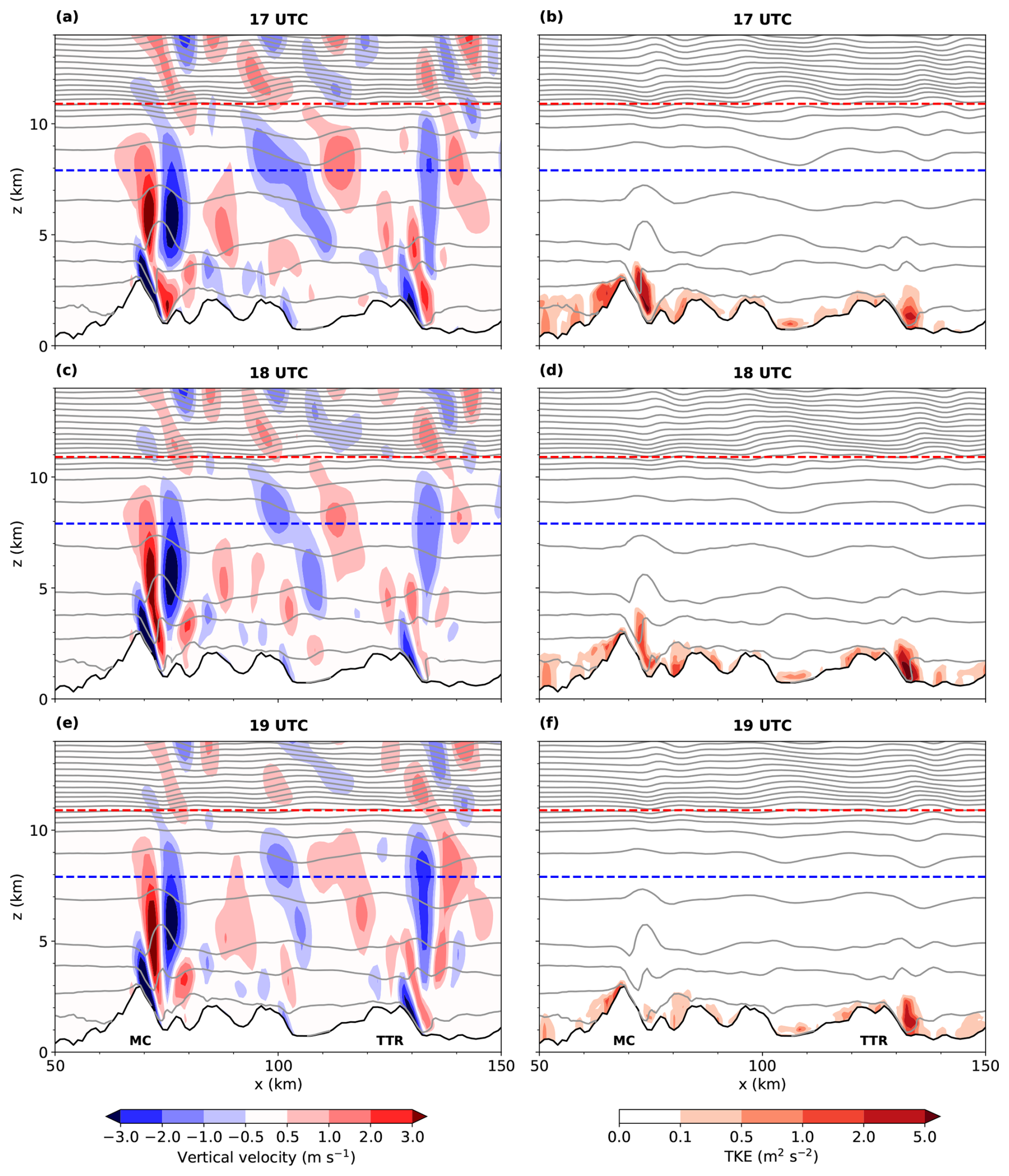
Figure 3 Vertical cross-sections of vertical wind (left column) and parameterized TKE (right column) over the southern segment of the flight track, simulated with I10-2TE at 17:00 UTC (a, b), 18:00 UTC (c, d), and 19:00 UTC (e, f). The similarity between the three times illustrates the quasi-stationary nature of the simulated wave field during the DEEPWAVE flight period. The blue dashed line denotes the lower flight leg, and the red dashed line the upper flight leg. Grey contours show potential temperature at 5 K spacing. The locations of Mount Cook (MC) and the Two Thumb Range (TTR) are indicated.

3.1 Reference simulation of the wave event

The reference simulation I10-2TE reproduces a distinct mountain-wave pattern over the South Island at flight time (18:00 UTC). Horizontal cross-sections of vertical velocity show alternating bands of ascent and descent downstream of the main ridge of the Southern Alps, extending from the mid-troposphere into the lower stratosphere (Fig. 2). The wave signal is most pronounced near the southern leg and south of the DEEPWAVE flight track. It is stronger in the troposphere (4 and 8 km) than in the lower stratosphere (11 km). This decrease in amplitude with height reflects partial wave trapping, consistent with the Scorer-parameter analysis in Sect. 3.2 (Fig. 7). Note that the dominant waves also increase in horizontal scale between 4 and 8 km.

A vertical cross-section along the southern segment of the flight path at 18:00 UTC highlights the primary wave response above the topography (Fig. 3c). The transect passes near Mount Cook, New Zealand's highest mountain, at about x = 68 km. Further southeast, at about x = 125 km, it crosses the Two Thumb Range, the last major ridge in this section. A strong mountain wave, with vertical velocities exceeding 3 m s⁻¹, is triggered by the Mount Cook region, while a weaker wave develops above the Two Thumb Range. Both waves propagate into the lower stratosphere and are associated with leeside descent, low-level steepening of the isentropes, and the production of turbulence (subgrid-scale TKE) as seen in Fig. 3d. Significant turbulence is confined to the ABL and to regions of steep isentropes associated with lee-side flow separation. Note that non-orographic ABL turbulence is weak, as expected for the early morning hours (06:00 local time).

To assess the stationarity of the simulated wave field, the same cross-section is shown at 17:00 and 19:00 UTC (Fig. 3a, b, e, f). At upper levels, the primary wave over Mount Cook remains largely unchanged, whereas noticeable differences appear further downstream above the Two Thumb Range. Near the surface, the flow over Mount Cook varies between the three times, with associated variations in the parameterized TKE. In summary, the large-scale wave pattern over the Mount Cook region is quasi-stationary, whereas smaller-scale features and the low-level TKE show less stationarity. This temporal variability at lower levels has little effect on the wave maxima near 6 km or the flight-leg altitudes.

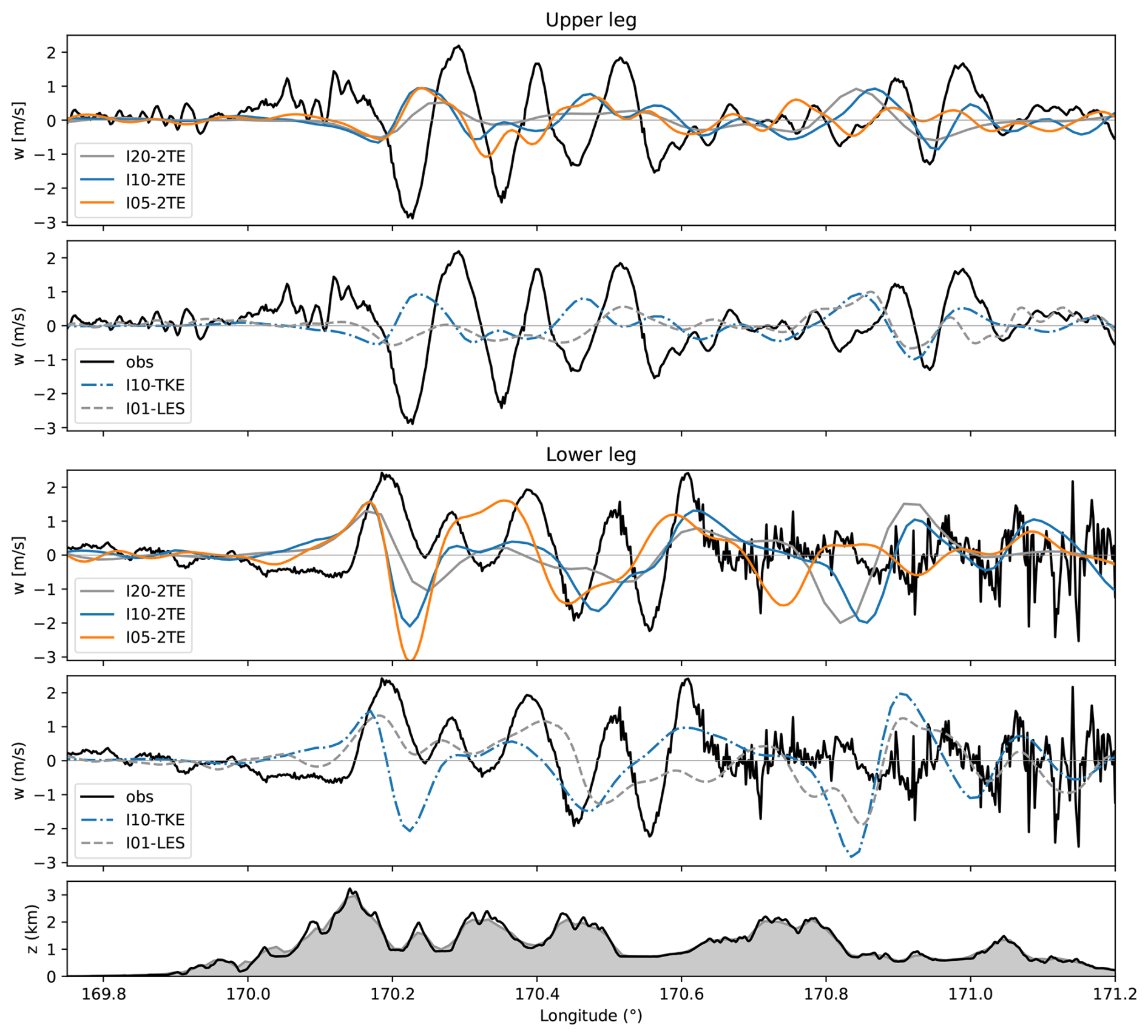
Figure 4 Comparison of vertical velocity from ICON simulations at different horizontal resolutions at 18:00 UTC with in situ observations along the southern segment of the flight track. Results are shown separately for the lower and upper flight legs, together with the underlying terrain along the cross-section, shown for I10-2TE (shading) and I01-LES (black line). Note that 0.2° on the horizontal axis corresponds to 16 km.

Comparison of I10-2TE with observations (Fig. 4) shows that the simulated wave amplitude, in terms of vertical velocity perturbations, agrees reasonably well with the observations on the lower flight leg but it is underestimated on the upper leg. A spatial phase mismatch between simulated and observed waves is also apparent, which is to be expected. While the simulated wave field is almost stationary, particularly for the strong wave triggered above Mount Cook, the real atmosphere is likely much less stationary due to multi-scale interactions among a spectrum of gravity waves and turbulent motions. Additional variability is also expected from temporal changes in the upstream profile. Note that the observed wave phases differ between the lower and upper flight legs. These differences are unlikely to reflect a vertical discontinuity; instead, they most likely result from the roughly one-hour time difference between the two legs and the non-stationary nature of the real gravity-wave field.

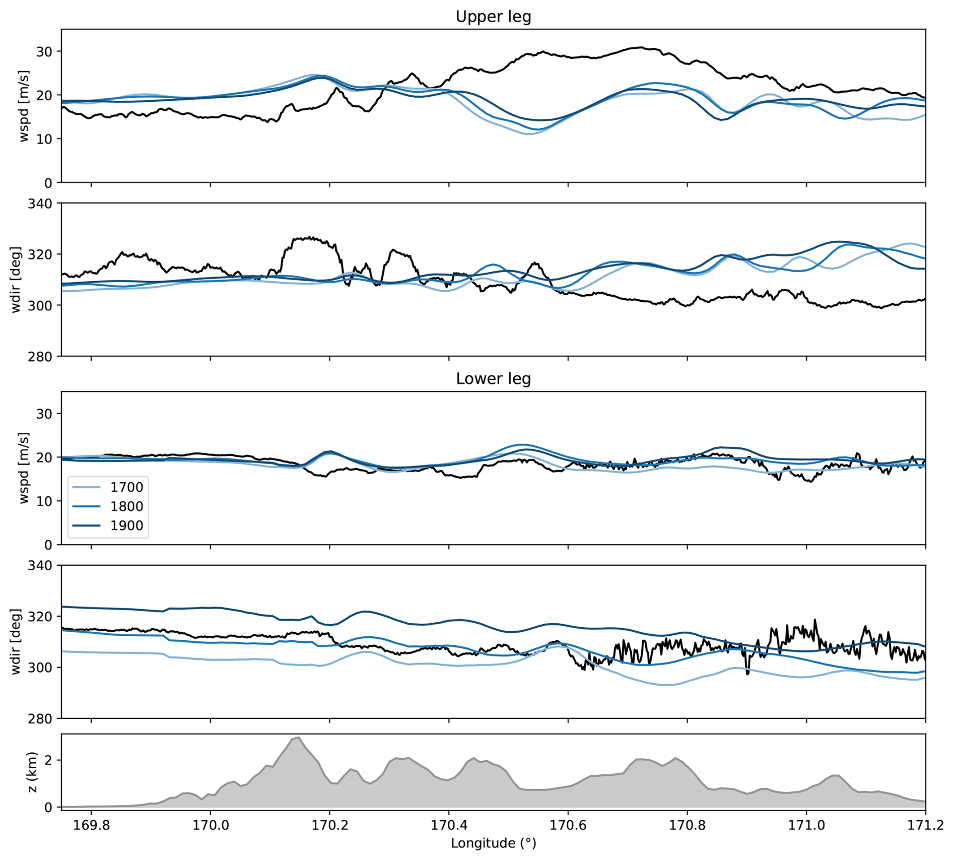
Figure 5 Comparison of horizontal wind speed and direction from the reference simulation I10-2TE at 17:00, 18:00, and 19:00 UTC with in situ observations along the southern segment of the flight track (lower leg: 17:30–17:50 UTC, upper leg: 18:47–19:07 UTC). Results are shown separately for the lower and upper flight legs, together with the underlying terrain along the cross-section.

The horizontal wind along both legs is compared with the observations in Fig. 5 for the reference simulation I10-2TE at 17:00, 18:00, and 19:00 UTC. The simulated wind direction on the lower leg changes by about 10° h⁻¹, and the simulation agrees most closely with the observations at the output times nearest each crossing (18:00 UTC for the lower leg, 19:00 UTC for the upper leg). The upper-level wind-speed bias (up to about 10 m s⁻¹) is common to all resolutions and to both turbulence schemes (not shown, as the winds are largely insensitive to scheme and resolution), so the upper-leg differences reflect the represented flow rather than the turbulence parameterization, consistent with the nearly identical resolved variances of the two schemes (Sect. 3.4). Part of the observed wind fluctuation is the wave itself (e.g., wind-speed perturbations of about 5 m s⁻¹ and wind-direction perturbations of 10–15° on the upper leg).

In summary, the reference simulation captures a strong vertically propagating mountain wave but shows no evidence of significant wave breaking or turbulence at flight altitudes associated with the dominant wave, consistent with the observations. It provides the baseline for assessing the sensitivity to model resolution and turbulence parameterization presented in the following subsections.

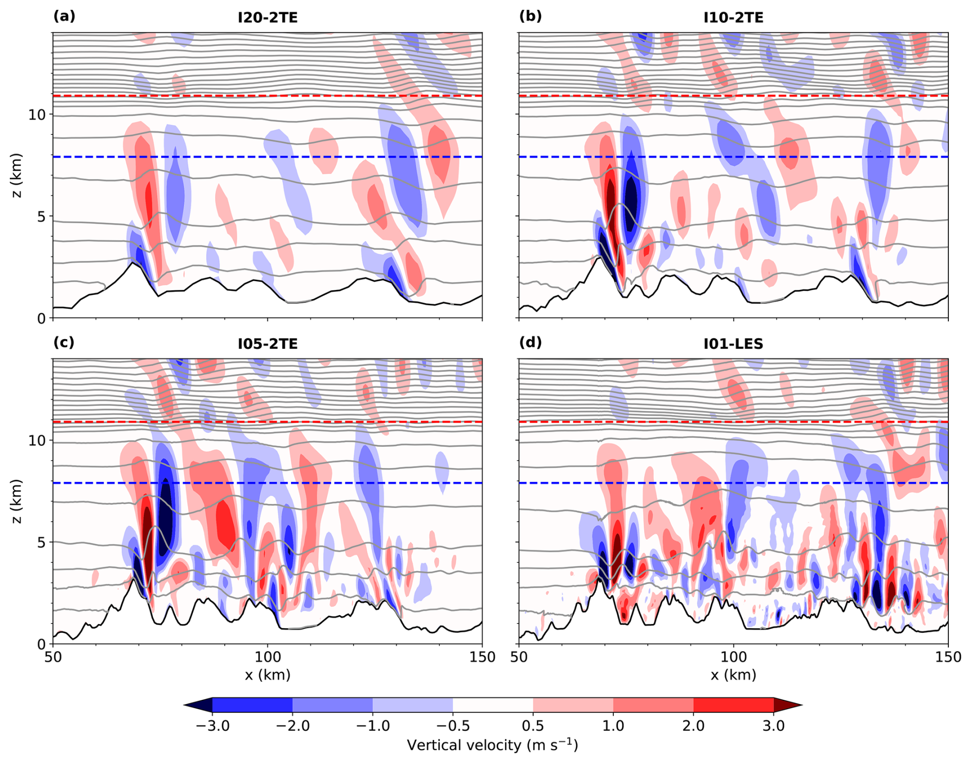
Figure 6 Comparison of vertical velocity along the southern flight-path transect at 18:00 UTC for 2TE simulations and LES at different horizontal resolutions: (a) 2 km, (b) 1 km, (c) 500 m, and (d) 130 m.

3.2 Sensitivity to horizontal and vertical resolution

Figure 6 presents the wave field in terms of vertical velocity and potential temperature. The simulated wave field is strongly affected by horizontal resolution, with substantially more wave activity at finer grid spacing. At 2 km resolution, the horizontal wavelength increases and the gravity wave exhibits a more hydrostatic character, as shorter scales are no longer resolved. This is particularly evident for the wave triggered by the Two Thumb Range. At finer resolution (0.5 km), the waves become more non-hydrostatic, with vertical velocity perturbations more vertically aligned. Importantly, the number of resolved waves increases as the model begins to capture shorter wavelengths. This effect is even more pronounced in the LES at 130 m. The LES further shows that the shortest wavelengths are trapped in the layer of enhanced stability below about 5 km, with a clear example of trapped lee waves in the lee of the Two Thumb Range. Another notable difference between the NWP simulations and the LES is the representation of the flow structure immediately downstream of the mountains (Mount Cook, an intermediate ridge at ∼ 100 km, and the Two Thumb Range). In the NWP runs, the downslope flow penetrates to lower levels than in the LES, which has a significant effect on mountain-wave triggering. These differences are likely due not only to resolution, but also to the different representation of the atmospheric boundary layer and its coupling with the mountain wave (e.g., Jiang et al., 2008). For completeness, horizontal cross-sections of the flow at different resolutions are shown in Appendix B, confirming the sensitivity of dominant gravity-wave scales to model resolution.

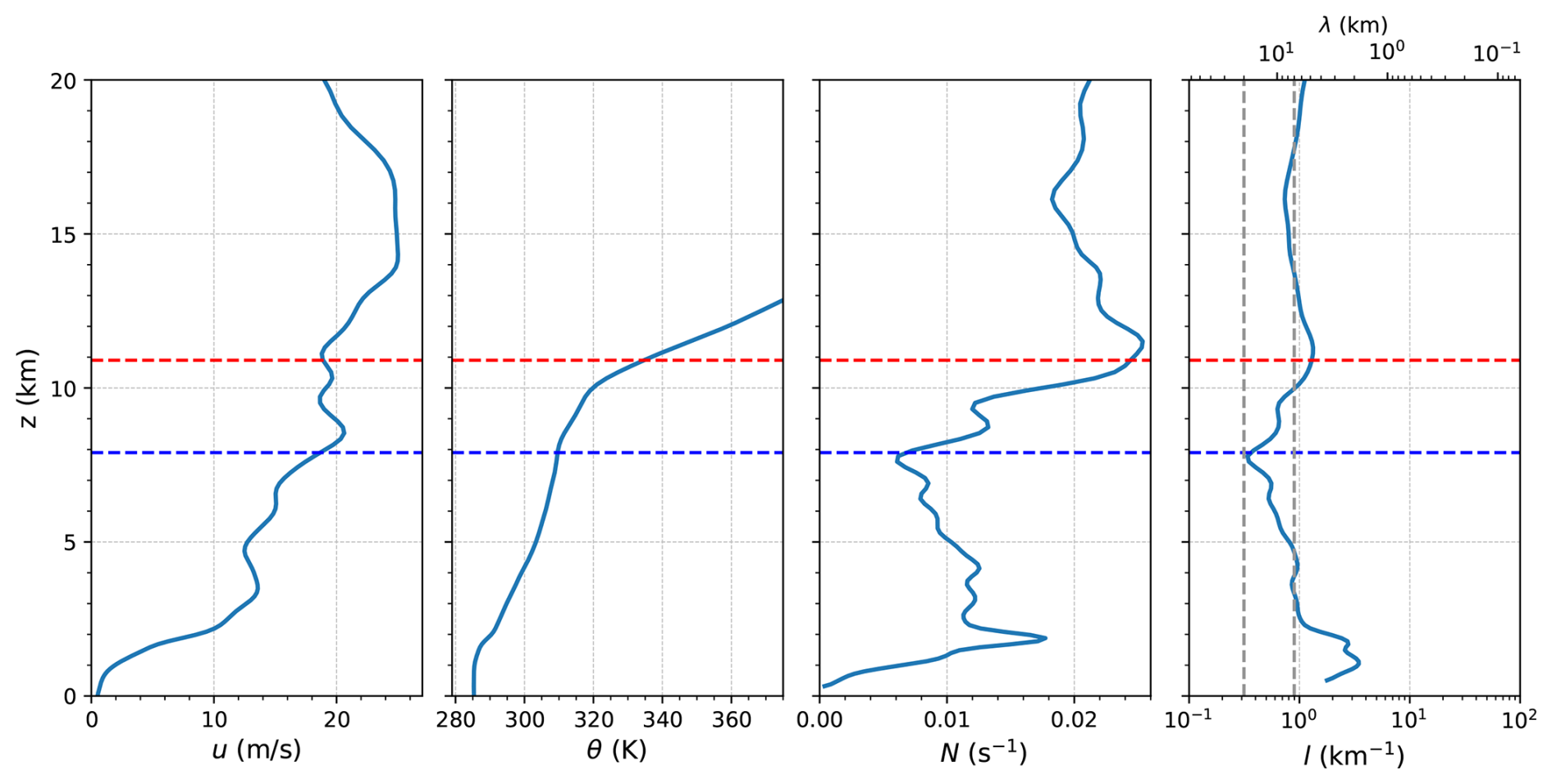
Figure 7 Upstream profiles of wind speed parallel to the southern flight leg (u), potential temperature (θ), Brunt–Väisälä frequency (N), and Scorer parameter (l) from the I10-2TE simulation. Profiles are taken at 10 km along the red transect line shown in Fig. 1 at 18:00 UTC. Wind speed and potential temperature are smoothed vertically using a Gaussian filter with a standard deviation of 1.5 vertical grid points. The grey vertical dashed lines indicate Scorer-parameter values corresponding to wavelengths of 7 and 20 km, respectively.

To gain further insight into the wave environment, upstream profiles of wind speed, potential temperature, Brunt–Väisälä frequency, and the Scorer parameter are shown in Fig. 7. Wind speed increases approximately linearly from about 10 m s⁻¹ at ridge height to nearly 20 m s⁻¹ just below the tropopause at 9 km. In terms of stability, the lower troposphere (below 5 km) is markedly more stable than the upper troposphere above. These two factors combine to produce a decrease of the Scorer parameter with height through much of the troposphere, followed by a recovery to slightly larger values in the lowermost stratosphere. The Scorer parameter profile implies a cut-off wavelength of about 7 km just above ridge level, increasing to roughly 20 km near the tropopause. This vertical structure explains the generation of trapped lee waves in the more stable layer below 5 km and is likely responsible for the reduced simulated wave amplitude at the upper flight leg. In the observations, by contrast, the primary wave keeps a nearly constant horizontal wavelength of about 8 km and a strong signal on the upper leg, indicating that it propagates more freely than the model's Scorer profile would suggest. This difference may in part reflect a bias in the simulated upstream wind and stability profile, which sets the Scorer parameter. Comparison of these simulations with in situ observations along the southern leg (Fig. 4) shows that the wave amplitude is reproduced reasonably well on the lower flight leg but underestimated on the upper leg. Among the NWP simulations, the 0.5 km run (I05-2TE) agrees best with the observed amplitudes at the lower level. The LES better reproduces the wavelength and phase than the NWP simulations, but underestimates the amplitude, particularly on the upper leg. These discrepancies likely reflect, among other factors, the non-stationarity of the real wave field compared to the quasi-stationary model simulations. For example, in the 0.5 km run, the simulated wave above Mount Cook at the altitude of the lower flight leg compares reasonably well with the observed wave at the altitude of the upper leg. The underestimation of the simulated amplitude aloft is most likely a matter of wave propagation (as discussed above), not of turbulent dissipation. Given the three-dimensional, multi-scale orography, exact agreement is not expected, in particular downstream of the primary wave, where waves from different ridges interfere.

The sensitivity to vertical resolution was assessed with additional 2TE runs in which the maximum grid spacing below 14 km was set to 400, 200, and 100 m, respectively. The coarsest grid (400 m) shows clear differences from the reference run, particularly in the stratosphere, whereas the 200 and 100 m results are very similar, particularly for the primary mountain wave, indicating near-convergence at 200 m (Fig. C1). This finding motivated the choice of a maximum vertical spacing of 200 m as the default in the NWP setup used here.

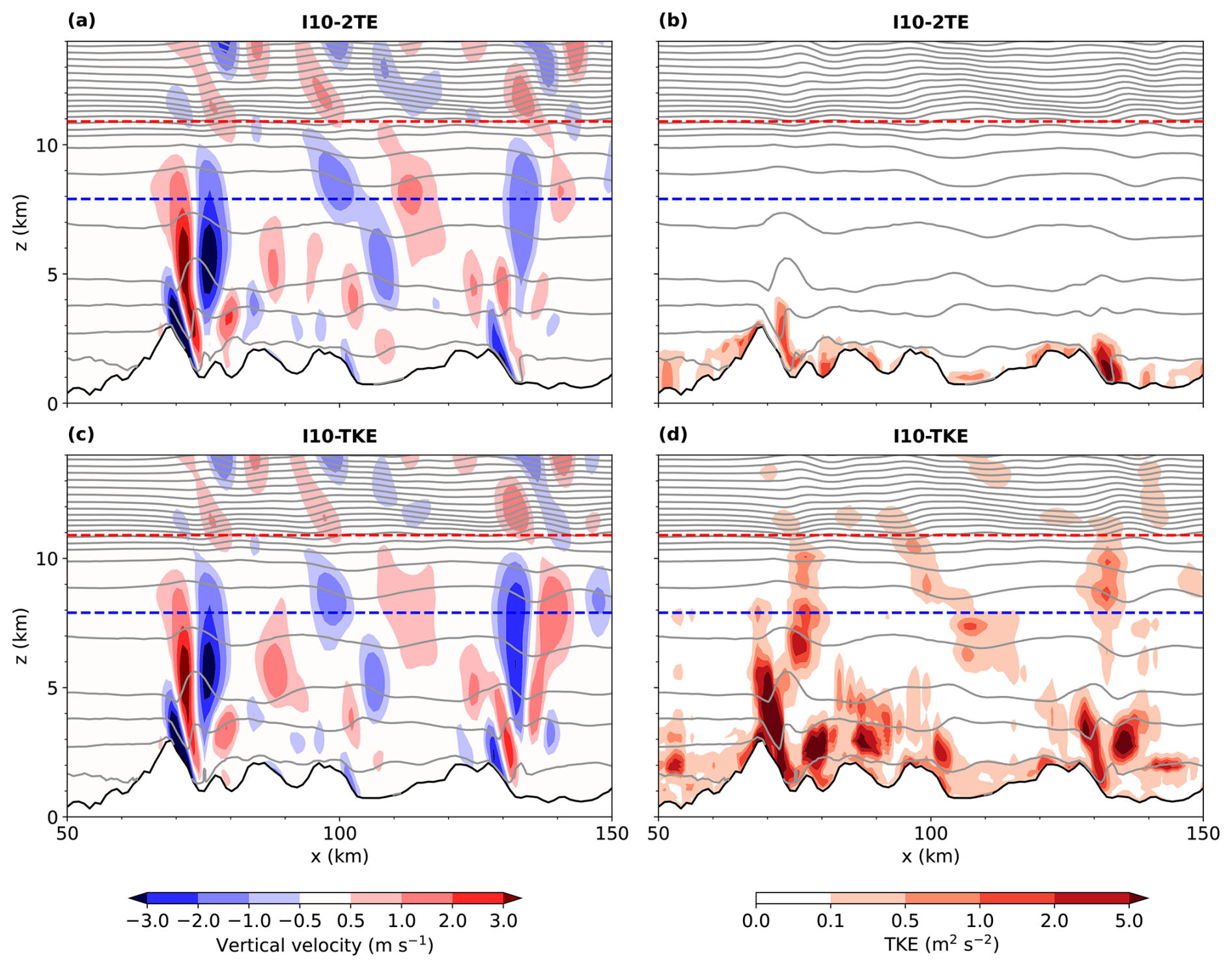
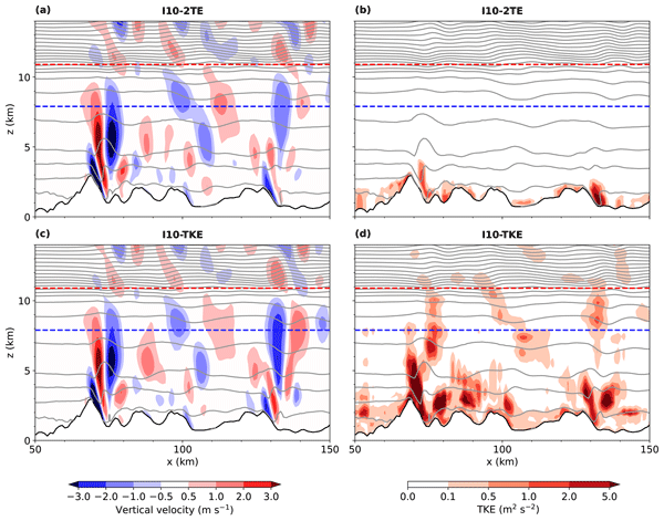
Figure 8 Comparison of vertical velocity and TKE along the southern flight-path transect at 18:00 UTC for ICON simulations at 1 km resolution using (a, b) the 2TE scheme and (c, d) the TKE scheme.

3.3 Sensitivity to turbulence parameterization

3.3.1 Comparison of the two turbulence schemes

At 1 km resolution, the two turbulence schemes produce rather similar wave patterns, particularly for the wave field above Mount Cook (Fig. 8a and c), as also seen in the horizontal cross-sections (Fig. B2). In contrast, the simulated TKE differs markedly between the schemes (Fig. 8b and d). The TKE scheme produces substantially higher TKE values throughout the wave field, whereas the 2TE scheme confines turbulence mainly to the ABL and the strongest low-level mountain waves. Given that wave trapping (Sect. 3.1 and 3.2), rather than turbulent dissipation, is the likely cause of the amplitude weakening aloft, the elevated TKE values above the ABL and outside regions of strong gravity-wave activity appear questionable and warrant further investigation. A key difference between the two schemes is the inclusion of additional empirical source terms in the TKE scheme (see Appendix A). This motivated further experiments to isolate the impact of these terms.

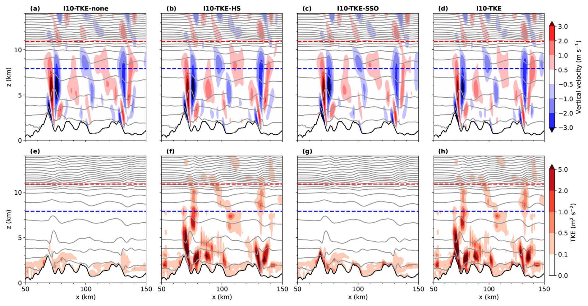
Figure 9 Comparison of vertical velocity and TKE along the southern flight-path transect at 18:00 UTC for ICON simulations using the TKE scheme: (a, e) both horizontal shear (HS) and subgrid-scale orography (SSO) deactivated, (b, f) HS activated, (c, g) SSO activated, and (d, h)  both HS and SSO activated (standard operational configuration).

3.3.2 Effect of optional TKE source terms in the TKE scheme

Sensitivity experiments with individual source terms switched off are shown in Fig. 9. These targeted experiments allow us to disentangle the effects of the horizontal shear and subgrid-scale orography source terms in the TKE equation (see Appendix A). While there are striking differences in the TKE fields, the resolved wave structures are almost identical across all four simulations. In I10-TKE and I10-TKE-HS, which both include the horizontal shear term, substantial TKE appears not only in the ABL and low-level flow-separation regions but also in patches throughout the troposphere, with weaker pockets even extending into the lower stratosphere. In contrast, I10-TKE-none and I10-TKE-SSO, which exclude the horizontal shear term, produce TKE distributions more similar to those obtained with the 2TE scheme, with a modest increase in TKE at low levels for I10-TKE-SSO. The occurrence of large TKE values in regions without obvious wave breaking suggests a breakdown of the empirical horizontal-shear parameterization at km-scale resolution. The parameterization is a two-dimensional Smagorinsky-type closure (Appendix A) that relates horizontal-shear production to the deformation of the resolved flow. Its physical interpretation assumes that deformation near the model cutoff is associated, on average, with a net downscale transfer of kinetic energy to unresolved motions. This interpretation is most plausible when near-grid variability is dominated by stratified mesoscale turbulence, as may occur in strongly deformational frontal and jet regions. In the present simulations, however, much of the grid-scale deformation is associated with resolved, coherent gravity waves. The closure cannot distinguish this largely reversible wave deformation from strain associated with an irreversible turbulent cascade and therefore converts wave-related deformation into parameterized TKE production. This explains why the excess TKE is spatially correlated with the resolved wave field rather than with regions of active turbulence. This finding is consistent with Bramberger et al. (2020), who showed that the Graphical Turbulence Guidance tool, which uses a similar empirical formulation, overpredicted turbulence magnitude over a large area during a breaking mountain-wave event over Iceland. This does not imply that low TKE is realistic everywhere. Two distinct deficiencies coexist at these resolutions: the horizontal shear term over-produces TKE where the observations show no turbulence (e.g., smooth spatial variation of w over the upstream half of the flight segment in Fig. 4), whereas genuine small-scale turbulence (e.g., downstream of the Two Thumb Range, and at the sub-km scales identified by Lachnitt et al., 2023) is under-resolved and hence missed by all configurations, including the LES.

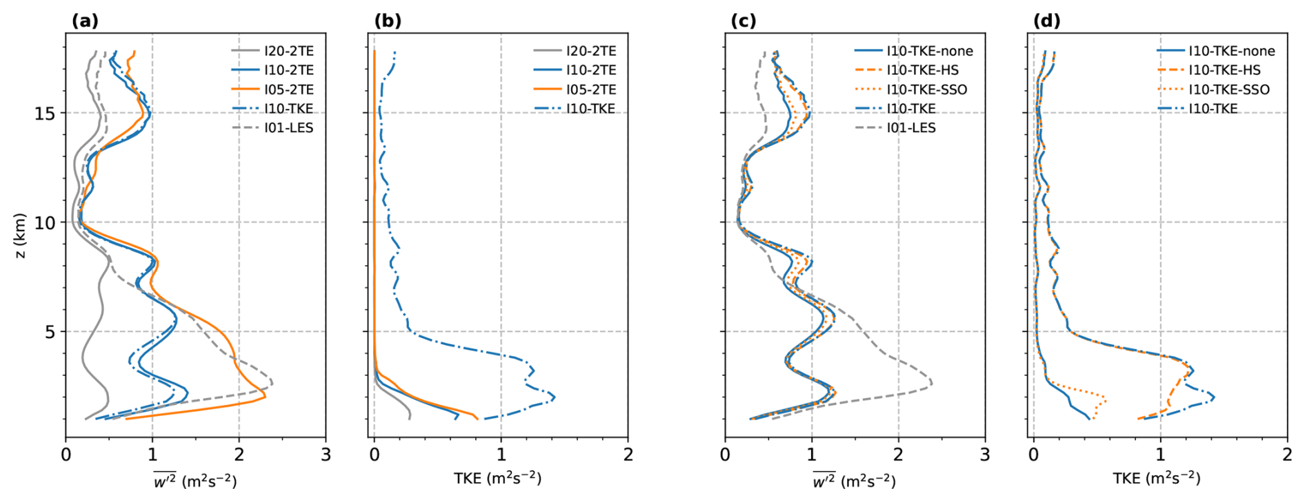
Figure 10 Profiles of resolved vertical velocity variance ($\stackrel{\mathrm{‾}}{w^{\prime \mathrm{2}}}$) and parameterized TKE, averaged over the analysis subdomain shown in Fig. 1, at 18:00 UTC for (a, b) different horizontal resolutions using the 2TE scheme and I10-TKE and (c, d) different TKE-scheme configurations, together with the LES.

3.4 Bulk properties of the GW field

3.4.1 Vertical velocity variance and TKE

Domain-averaged profiles of resolved vertical velocity variance ($\stackrel{\mathrm{‾}}{w^{\prime \mathrm{2}}}$) and parameterized TKE highlight important differences in how resolution and turbulence schemes represent small-scale energy (Fig. 10). Among the 2TE simulations, the 0.5 km run performs particularly well: its variance profile aligns closely with the LES in the lower troposphere, indicating that fine-scale vertical motions are reasonably captured at this resolution. In contrast, coarser runs at 1 and 2 km systematically underestimate the variance, with the largest discrepancy below 5 km in the layer containing the trapped lee waves. This highlights that quasi-LES resolutions of a few hundred meters are required to reproduce the vertical distribution of wave-induced resolved variance for this mountain wave event, which included low-level trapped lee waves.

Above the layer of trapped lee waves, the two simulations I10-2TE and I05-2TE agree very well, indicating near convergence with respect to the resolved variance associated with the dominant mountain waves. While the LES may be a more realistic reference at lower heights due to its improved representation of short-scale trapped lee waves, this is likely less true in the upper troposphere, where comparison with observations indicates that the LES underestimates the magnitude of the vertical velocity fluctuations. This is consistent with an over-dissipation of the near-grid-scale wave amplitude by the LES subgrid closure at marginal resolution: the LES resolves the wavelength and phase but damps the amplitude of the shortest resolved waves. The LES is therefore not automatically the more realistic reference.

At 1 km resolution, the resolved variances ($\stackrel{\mathrm{‾}}{w^{\prime \mathrm{2}}}$) are broadly similar between the two turbulence schemes, but the TKE fields differ substantially. Simulations with the TKE scheme generate larger TKE values than those with the 2TE scheme, particularly when the horizontal shear term is active (the default setup of the scheme). These inflated values contrast with the more realistic profiles from the 2TE simulations and from the TKE scheme without the empirical shear term. Together, these findings emphasize that, while resolved variances converge toward LES at sufficiently fine resolution, the representation of TKE remains highly sensitive to the choice of turbulence formulation.

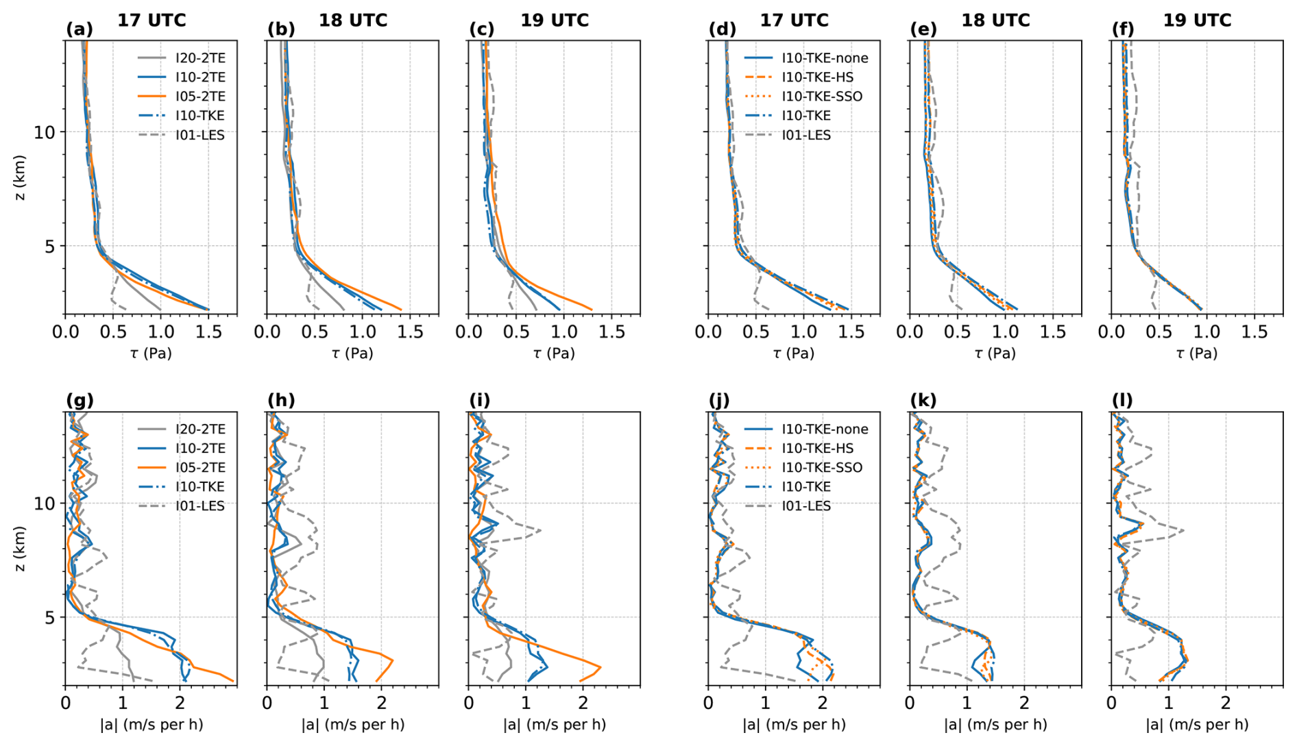
Figure 11 Top row: Profiles of area-averaged momentum flux, τ, for (a–c) different horizontal resolutions using the 2TE scheme and I10-TKE, and (d–f) different TKE-scheme configurations, at three consecutive times, together with the LES. Fluxes are calculated within the same analysis subdomain as in Fig. 10, after interpolation to regular vertical levels with 200 m spacing, and are shown above 2.2 km. Bottom row: As for the top row, but profiles of the momentum-flux divergence, expressed in terms of the magnitude of the corresponding acceleration, computed by vertical differencing at 300 m spacing.

3.4.2 Wave momentum fluxes

Domain-averaged profiles of vertical momentum flux and its vertical divergence (the wave drag) at three consecutive times illustrate how resolution and turbulence schemes influence the representation of wave-induced transport (Fig. 11). Profiles are shown above 2.2 km, where fewer than 5 % of subdomain grid columns lie below the surface; at lower levels the increasing terrain-masked fraction would bias the area average and, in particular, its vertical derivative. The flux divergence is computed by differencing at 300 m spacing, coarser than the 200 m flux grid, to suppress noise amplification by the derivative. In the 2TE simulations, the low-level momentum flux increases with increasing resolution as the orography is better resolved. At 17:00 UTC, the flux profiles for the two higher-resolution simulations, I10-2TE and I05-2TE, are nearly identical. By 18:00 UTC, a significant difference between the two simulations has emerged below 3–4 km, which persists, and becomes more pronounced, at 19:00 UTC. This growing discrepancy with time parallels the reduced stationarity of the low-level wave field noted in Sect. 3.1, and is consistent with the resolution sensitivity of the resolved variance in the trapped-lee-wave layer found in Sect. 3.4.1. The flux divergence (Fig. 11, bottom row) already differs between I10-2TE and I05-2TE at 17:00 UTC. The momentum flux profile for I10-TKE is very close to that for I10-2TE for all three times, despite the large differences in TKE between the two schemes. This suggests that the empirical horizontal shear term in the TKE scheme inflates the TKE but has little influence on the bulk momentum flux. The flux divergence is similarly insensitive to the horizontal-shear term (Fig. 11d–f): the additional TKE is not accompanied by a corresponding momentum deposition. Turbulence production associated with wave breaking would leave a signature in the drag; the horizontal-shear TKE does not. We interpret this decoupling as further evidence that the additional TKE is spurious.

Overall, the results highlight that area-averaged quantities, such as the area-averaged momentum flux, generally exhibit a more robust and monotonic behavior with increasing resolution than local quantities such as vertical velocity or local TKE fields. Local fields are strongly influenced by phase shifts, small-scale variability, and non-stationarity, making convergence assessments more difficult and less meaningful. In contrast, spatial averaging reduces this sensitivity and therefore provides a clearer indication of resolution effects, making momentum flux a more robust diagnostic for evaluating mountain-wave simulations.

4 Conclusions

This study investigated the simulation of mountain waves with the ICON model, focusing on the influence of horizontal and vertical resolution and the representation of turbulence through different parameterization schemes. We examined the performance of the newly implemented two-energy scheme (2TE scheme) in reproducing mountain-wave structures and associated turbulence during a case from the DEEPWAVE campaign over New Zealand on 12 July 2014. Model simulations were compared with high-frequency aircraft observations and a nested LES run for detailed visual and statistical evaluation.

Our results demonstrated that both vertical and horizontal resolutions play a critical role in accurately capturing the structure and behavior of mountain waves. We find that a vertical grid spacing of less than 200 m or less is necessary to adequately resolve the wave field in the UTLS region (Fig. C1). Insufficient vertical resolution damps the wave amplitude, leading to underestimation of wave strength. With respect to horizontal resolution, simulations at 0.5 km approached the LES in terms of wavelength, while coarser runs (1–2 km) underestimated the number and detail of shorter-scale waves. The area-averaged momentum flux, a target diagnostic for GW-drag parameterization, showed a corresponding resolution sensitivity: at low levels it continued to increase between 1 km and 500 m, indicating that the bulk momentum budget has not yet converged at these resolutions. Differences between NWP and LES simulations also point to the importance of how the ABL is represented, as ABL coupling affects lee-side flow separation, and thus the triggering of mountain waves.

Comparison with observations shows, however, that the LES is not automatically more realistic. While the LES may be a more realistic reference at lower heights due to its improved representation of orography and short-scale trapped lee waves, this is likely less true in the upper troposphere, where comparison with observations indicates that the LES underestimates the magnitude of the vertical velocity fluctuations. This may reflect that turbulence and wave breaking remain under-resolved even at 130 m resolution, leading to excessive damping of wave amplitudes.

The two turbulence schemes produced very similar resolved wave fields and comparable area-averaged momentum-flux profiles, but differed strongly in parameterized TKE. This difference originates in the empirical horizontal-shear source term of the operational TKE-scheme configuration, which produces spurious TKE at km-scale resolution, as shown by the controlled source-term experiments (Fig. 9) and by the scaling of the term (Appendix A). The 2TE scheme reproduces the resolved wave field as well as the operational scheme, remains numerically well behaved in the strongly stratified UTLS, and does not exhibit this artifact, which makes it a viable alternative for such applications. We do not, however, claim that the 2TE scheme is more accurate in representing turbulence. That a substantial part of the gravity-wave field in this case is non-breaking, including the primary wave at flight level, is what makes the spurious horizontal-shear TKE clearly identifiable: no significant turbulence is expected in such regions, and none is observed.

Although differences in the resolved flow fields are comparatively small, an accurate representation of TKE is critical for many applications, including aviation turbulence forecasting and the transport and dispersion of tracers such as greenhouse gases and air pollutants. Spurious or overly damped turbulence can directly affect estimates of mixing and exchange between atmospheric layers.

Hence, our findings suggest that careful reevaluation of turbulence parameterizations is required when using high-resolution NWP models in mountainous terrain. For km-scale resolutions, model setups should consider disabling or tuning the horizontal shear and SSO terms in the TKE scheme to avoid spurious TKE production. Alternatively, schemes such as 2TE provide a promising framework for turbulence representation at these scales.

The results have important implications for the configuration of high-resolution regional weather models and for advancing the understanding of terrain-induced gravity waves and associated turbulent processes. Future work will extend this analysis to additional DEEPWAVE cases and other campaigns to test the robustness of these conclusions. A further priority is coupling the 2TE scheme with gravity-wave parameterizations to bridge explicitly resolved and parameterized wave–turbulence interactions, particularly in global and climate modeling frameworks.

Appendix A: Overview of the TKE and 2TE turbulence schemes in ICON

A1 TKE budget and the operational ICON TKE scheme

The general form of the TKE budget equation in a coordinate system aligned with the mean wind, under horizontal homogeneity and negligible subsidence, is

$$\begin{array}{}\text{(A1)}& \begin{array}{rl}\underset{\mathrm{I}}{\underbrace{{\displaystyle \frac{\partial \stackrel{\mathrm{‾}}{e}}{\partial t}}}}=& \underset{\text{II}}{\underbrace{{\displaystyle \frac{g}{\stackrel{\mathrm{‾}}{{\mathit{\theta }}_v}}}\left(\stackrel{\mathrm{‾}}{w^{\prime }{\mathit{\theta }}_v^{\prime }}\right)}}-\underset{\text{III}}{\underbrace{\stackrel{\mathrm{‾}}{u^{\prime }{w}^{\prime }}{\displaystyle \frac{\partial U}{\partial z}}}}-\underset{\text{IV}}{\underbrace{{\displaystyle \frac{\partial \left(\stackrel{\mathrm{‾}}{w^{\prime }e}\right)}{\partial z}}}}-\underset{\text{V}}{\underbrace{{\displaystyle \frac{\mathrm{1}}{\stackrel{\mathrm{‾}}{\mathit{\rho }}}}{\displaystyle \frac{\partial \left(\stackrel{\mathrm{‾}}{w^{\prime }{p}^{\prime }}\right)}{\partial z}}}}\\ & -\underset{\text{VI}}{\underbrace{\mathit{\epsilon },}}\end{array}\end{array}$$

where term I represents the local tendency of TKE; term II the buoyancy production or destruction; term III the shear production; term IV the turbulent transport term; term V the pressure transport; and term VI the viscous dissipation rate (Stull, 1988).

The operational turbulence scheme in ICON (Raschendorfer, 2001) is based on this classical TKE framework but augments it by explicitly separating turbulence from other small-scale motions such as gravity-wave–induced momentum tendencies and horizontal deformation. The corresponding prognostic equation for TKE is

$$\begin{array}{}\text{(A2)}& \begin{array}{rl}{\displaystyle \frac{\partial (q^{\mathrm{2}}/\mathrm{2})}{\partial t}}=& \underset{\text{Buoyancy}}{\underbrace{\mathit{\beta }\stackrel{\mathrm{‾}}{w^{\prime }{\mathit{\theta }}_v^{\prime }}}}-\underset{\text{Vertical Shear}}{\underbrace{\left(\stackrel{\mathrm{‾}}{u_{\mathrm{1}}^{\prime }{w}^{\prime }}{\displaystyle \frac{\partial U_{\mathrm{1}}}{\partial z}}+\stackrel{\mathrm{‾}}{u_{\mathrm{2}}^{\prime }{w}^{\prime }}{\displaystyle \frac{\partial U_{\mathrm{2}}}{\partial z}}\right)}}\\ & +\underset{\text{Turbulent Transport}}{\underbrace{{\displaystyle \frac{\partial }{\partial z}}\left[{\mathit{\alpha }}_T\mathit{\lambda }q{\displaystyle \frac{\partial (q^{\mathrm{2}}/\mathrm{2})}{\partial z}}\right]}}-\underset{\text{Dissipation}}{\underbrace{{\displaystyle \frac{q^{\mathrm{3}}}{{\mathit{\alpha }}_{\mathrm{M}}\mathit{\lambda }}}}}\\ & +\underset{\text{Subgridscale Orography}}{\underbrace{U_{\mathrm{1}}{\displaystyle \frac{\partial U_{\mathrm{1}}}{\partial t}}{|}_{\text{SSO}}+U_{\mathrm{2}}{\displaystyle \frac{\partial U_{\mathrm{2}}}{\partial t}}{|}_{\text{SSO}}}}\\ & +\underset{\text{Horizontal Shear}}{\underbrace{S_{\mathrm{H}}.}}\end{array}\end{array}$$

Here, the subscripts 1 and 2 denote the two horizontal wind components (U₁, U₂) and $q=\sqrt{\mathrm{2}\stackrel{\mathrm{‾}}{e}}$ is the turbulent velocity scale. $\mathit{\beta }=g/\mathit{\theta }{\mathrm{̄}}_v$ is the buoyancy parameter, λ the turbulent length scale, and α_M and α_T are closure constants for dissipation and turbulent transport. The additional terms account for (i) contributions from the SSO parameterization, which represents drag and gravity-wave momentum deposition from unresolved topography; and (ii) turbulence generation associated with large-scale horizontal shear, deformation, and divergence (an empirical source term). The purpose of these extensions is to enable the turbulence closure to operate also in stable layers above the boundary layer and to provide diagnostic quantities such as the eddy dissipation rate (EDR), which is used in aviation turbulence applications (Goecke and Machulskaya, 2021).

The horizontal-shear source term follows a two-dimensional Smagorinsky-type closure (Goecke and Machulskaya, 2021) that relates the horizontal-shear production to the deformation of the resolved flow, under the assumption that this deformation is associated, on average, with a net downscale transfer of kinetic energy to unresolved turbulence,

$$\begin{array}{rl}& S_{\mathrm{H}}=l_{\mathrm{h}}^{\mathrm{2}}\sqrt{C^{\mathrm{3}}{\mathit{\alpha }}_{\mathrm{M}}}(\sqrt{{\text{DEF}}^{\mathrm{2}}+c_{\mathrm{1}}^{\mathrm{2}}{\text{DIV}}^{\mathrm{2}}}-c_{\mathrm{1}}\text{DIV}{)}^{\mathrm{3}},\\ & l_{\mathrm{h}}={\displaystyle \frac{a_{\mathrm{h}}l}{{\mathit{Ri}}^{\mathrm{2}/\mathrm{3}}}},a_{\mathrm{h}}=\mathrm{0.2},\end{array}$$

where DEF is the horizontal deformation, DIV the horizontal divergence, l the grid spacing, and C and c₁ tuning constants. The source therefore scales approximately as $S_{\mathrm{H}}\sim l^{\mathrm{2}}|{\mathrm{\nabla }}_{\mathrm{h}}U{|}^{\mathrm{3}}R{i}^{-\mathrm{4}/\mathrm{3}}$, i.e. as a grid-scale two-dimensional Smagorinsky production whose length scale is set by the grid spacing rather than by a physical turbulence scale. The applicability of this interpretation at km-scale resolution is discussed in Sect. 3.3.2.

Because these additional turbulence sources arise from parameterized processes rather than directly from the resolved flow, the resulting TKE tendencies may not always reflect the local dynamical response in situations dominated by wave propagation and breaking.

A2 Two-energy (2TE) scheme formulation

The 2TE scheme (Bašták Ďurán et al., 2022) provides a unified framework for representing turbulence, shallow convection, and subgrid-scale cloud processes. It introduces two prognostic energy equations: one for TKE and one for the total turbulence energy (TTE). The prognostic TKE equation is

$$\begin{array}{}\text{(A3)}& \begin{array}{rl}{\displaystyle \frac{\partial e_{\mathrm{k}}}{\partial t}}=& \underset{\text{Buoyancy\hspace{0.17em}\hspace{0.17em}(APDF)}}{\underbrace{{\displaystyle \frac{g}{{\mathit{\theta }}_{\mathrm{0}}}}\stackrel{\mathrm{‾}}{{\mathit{\theta }}_v^{\prime }{w}^{\prime }}}}-\underset{\text{Vertical\hspace{0.17em}\hspace{0.17em}Shear}}{\underbrace{\left(\stackrel{\mathrm{‾}}{u_{\mathrm{1}}^{\prime }{w}^{\prime }}{\displaystyle \frac{\partial U_{\mathrm{1}}}{\partial z}}+\stackrel{\mathrm{‾}}{u_{\mathrm{2}}^{\prime }{w}^{\prime }}{\displaystyle \frac{\partial U_{\mathrm{2}}}{\partial z}}\right)}}\\ & +\underset{\text{Turbulent\hspace{0.17em}\hspace{0.17em}Transport}}{\underbrace{{\displaystyle \frac{\partial }{\partial z}}\left(K_{e_{\mathrm{k}}}{\displaystyle \frac{\partial e_{\mathrm{k}}}{\partial z}}\right)}}-\underset{\text{Dissipation}}{\underbrace{{\displaystyle \frac{\mathrm{2}{e}_{\mathrm{k}}}{{\mathit{\tau }}_{\mathrm{k}}}}}}\end{array}\end{array}$$

and the accompanying equation for TTE is

$$\begin{array}{}\text{(A4)}& \begin{array}{rl}{\displaystyle \frac{\partial e_{\mathrm{s}}}{\partial t}}=& \left(\stackrel{\mathrm{‾}}{u_{\mathrm{1}}^{\prime }{w}^{\prime }}{\displaystyle \frac{\partial U_{\mathrm{1}}}{\partial z}}+\stackrel{\mathrm{‾}}{u_{\mathrm{2}}^{\prime }{w}^{\prime }}{\displaystyle \frac{\partial U_{\mathrm{2}}}{\partial z}}\right)+{\displaystyle \frac{\partial }{\partial z}}\left(K_{e_{\mathrm{s}}}{\displaystyle \frac{\partial e_{\mathrm{s}}}{\partial z}}\right)\\ & -{\displaystyle \frac{\mathrm{2}{e}_{\mathrm{s}}}{{\mathit{\tau }}_{\mathrm{s}}}},\end{array}\end{array}$$

where e_k is the turbulent kinetic energy (TKE), e_s the total turbulence energy (TTE), and τ_k, τ_s and $K_{e_{\mathrm{k}}}$, $K_{e_{\mathrm{s}}}$ are the corresponding dissipation time scales and diffusion coefficients.

A key feature of the scheme is the quasi-prognostic stability parameter ${\mathit{Ri}}_{\mathrm{f}}^{\ast }$, defined as a combination of a non-local and a local estimate of the flux Richardson number,

$$\begin{array}{}\text{(A5)}& {\mathit{Ri}}_{\mathrm{f}}^{\ast }=a{\mathit{Ri}}_{\mathrm{f}}^{\text{TE}}+(\mathrm{1}-a){\mathit{Ri}}_{\mathrm{f}}^{\text{GR}},\end{array}$$

where ${\mathit{Ri}}_{\mathrm{f}}^{\text{TE}}$ denotes the non-local estimate, calculated from the two prognostic turbulence energies (TKE and TTE), and ${\mathit{Ri}}_{\mathrm{f}}^{\text{GR}}$ denotes the local estimate, based on the turbulent Prandtl number and the local gradient Richardson number (see Eqs. (21) and (22) in Bašták Ďurán et al., 2022). This nonlinearity and non-locality help suppress the oscillatory behavior often encountered in classical TKE closures. In contrast to the TKE scheme, the mixing length in the 2TE scheme is dynamically adjusted based on the diagnosed ABL height and the bulk state of the ABL (convective versus stable). Another important aspect is the formulation of the stability functions, which do not rely on a critical gradient Richardson number. This guarantees realizability of the scheme over the full range of stratification conditions.

A notable technical property of the 2TE formulation is that it yields numerically stable solutions without requiring a prescribed minimum diffusion coefficient. This avoids the need for ad hoc lower bounds on vertical diffusivity that are often introduced to maintain numerical stability in classical TKE closures. Allowing diffusivities and mixing lengths to approach small values organically preserves the intended behavior of turbulence in weakly turbulent or strongly stratified layers. The 2TE scheme is coupled to the APDF framework for diagnosing buoyancy production. The APDF uses a double-Gaussian joint PDF of vertical velocity, liquid water potential temperature, and total water content. Although originally developed for cloud-topped boundary layers, this coupling ensures a consistent representation of buoyancy effects based on the diagnosed turbulent state. The practical value of retaining the APDF coupling in the UTLS is therefore its ability to represent subgrid-scale condensation, for example, thin, wave-induced cirrus, consistently with the rest of the scheme, should saturation be locally approached; the dry buoyancy flux itself is unaffected.

Focusing on the UTLS region, the most relevant characteristics of the 2TE scheme compared to the TKE scheme are: (i) the local–nonlocal stability parameter, which strongly reduces the occurrence of oscillations and thereby allows smaller exchange coefficients without risking numerical instability, thus preventing the overmixing that can erode thin stably stratified layers; and (ii) stability functions that guarantee realizability over the full range of gradient Richardson numbers.

Appendix B: Additional horizontal cross sections

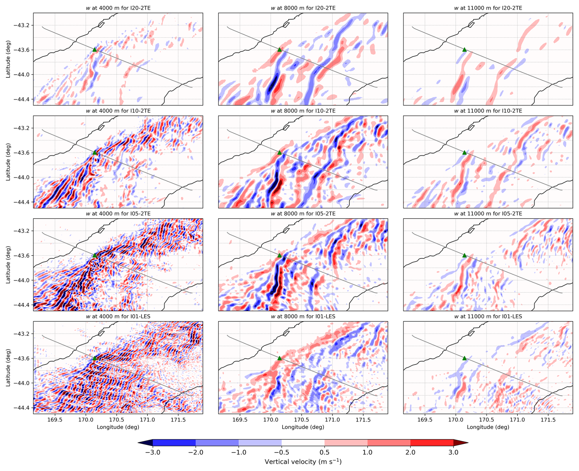
Figure B1 Horizontal cross-sections of vertical velocity at 4000 m (left column), 8000 m (middle), and 11 000 m (right), corresponding to a mid-tropospheric height and the lower and upper flight legs, respectively, for ICON simulations using the 2TE turbulence scheme at different horizontal resolutions, together with the LES.

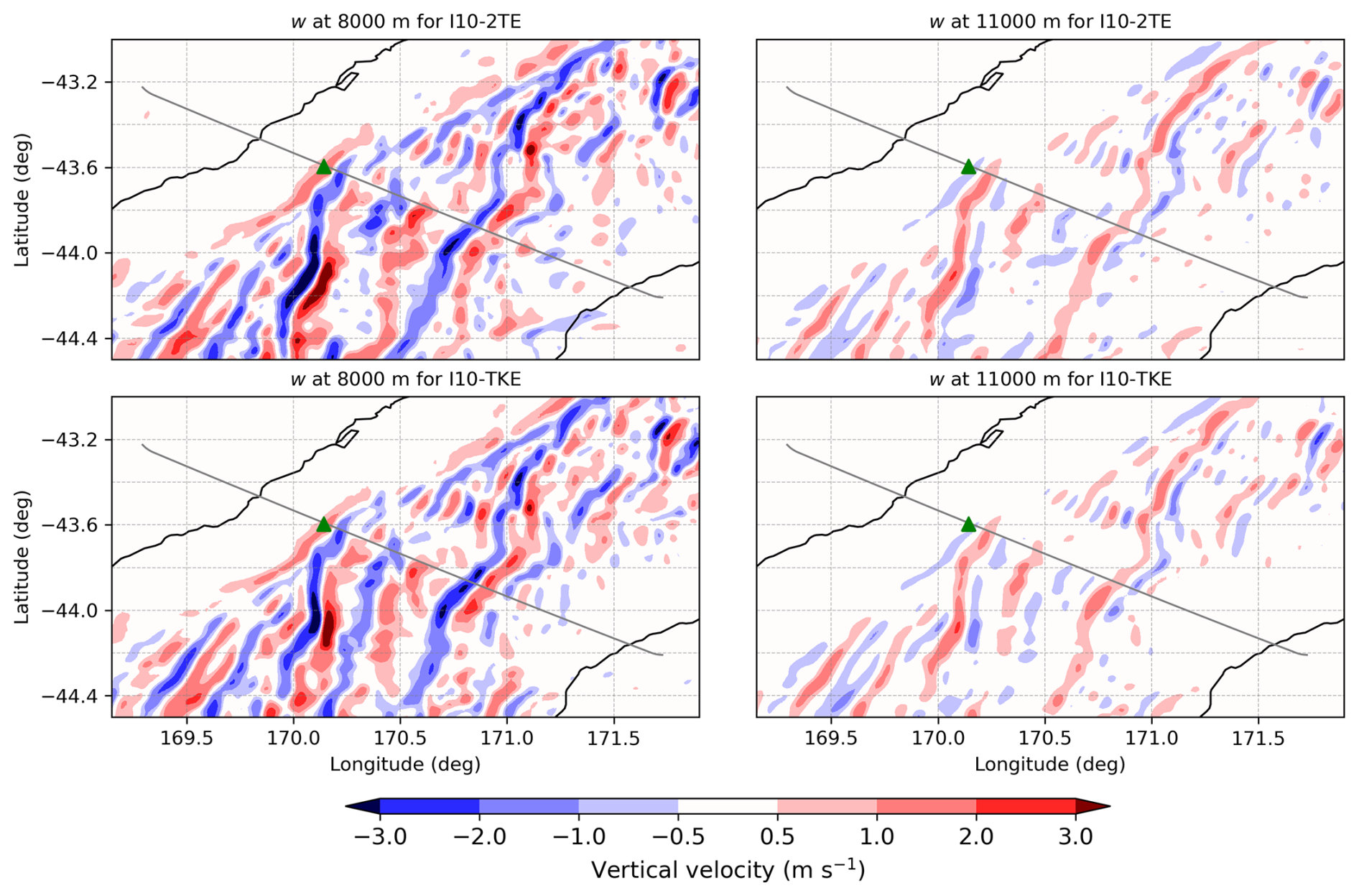
Figure B2 Horizontal cross-sections of vertical velocity at 8000 and 11 000 m, corresponding to the lower and upper flight legs, for the ICON simulations I10-2TE and I10-TKE. The two simulations produce broadly similar wave structures, indicating that differences between the schemes are primarily reflected in the parameterized TKE rather than in the resolved vertical velocity patterns.

Appendix C: Sensitivity to vertical resolution

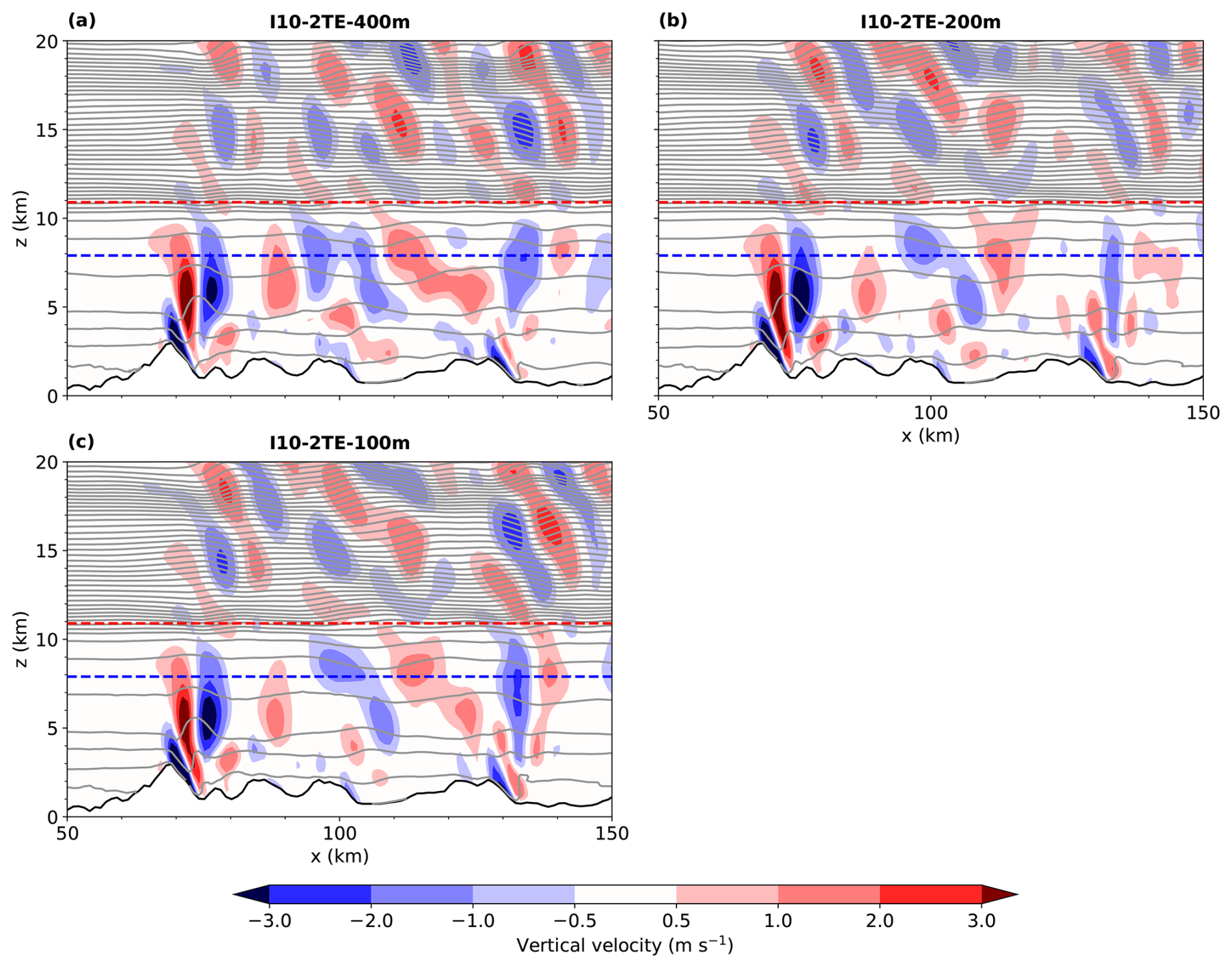
Figure C1 Vertical velocity (shaded) and potential temperature (contour lines) along the southern flight-path transect at 18:00 UTC for 1-km ICON simulations using the 2TE turbulence scheme at different maximum vertical grid spacings in the UTLS region: (a) 400 m, (b) 200 m, and (c) 100 m.