Secondary ice production within shallow, mixed-phase clouds in cold air outbreaks over the Labrador Sea

Shallow, mixed-phase clouds within marine cold air outbreaks (CAOs) frequently form over the North Atlantic. Their shortwave radiative effect is modulated as stratocumulus decks break up into cumulus clouds to the south. Microphysical processes controlling their phase remain poorly represented by climate models; of these, secondary ice production (SIP), describing mechanisms producing new ice crystals from existing primary ice, is a major contributor to uncertainties in the mixed-phase cloud response to future warming. We examine in-situ measurements of cloud microphysical properties made using the UK FAAM BAe-146 research aircraft within CAOs over the Labrador Sea as part of the October–November 2022 M-Phase field campaign. Measured ice particle concentrations frequently exceeded ice-nucleating particle (INP) concentrations at all in-cloud temperatures, highlighting the importance of SIP in these clouds. Peak ice concentrations were observed within the Hallett–Mossop (H–M) process temperature range (−3 to −8 °C), four orders of magnitude above expected INP concentrations. SIP regions contained large, rimed columns and graupel mixed with smaller columnar crystals (< 200 µm), indicative of the H–M process. Splinter production rate calculations indicated the H–M process could feasibly account for most ice production in the largest ice enhancement regions. A secondary zone of SIP activity, between −15 and −18 °C, comprised fragile, branched crystals, aggregates and ice fragments, consistent with laboratory studies of ice-ice collisional breakup. SIP amplified across the stratiform-to-convective regime transition, favouring weak-to-moderate updrafts (0 to +2 m s⁻¹) containing high concentrations of large liquid droplets, suggesting regime-aware SIP schemes would benefit future CAO modelling.

1 Introduction

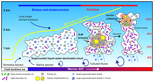
Marine cold air outbreaks (CAOs) are characterised by the advection of cold, polar air over relatively warm, open ocean (Papritz et al., 2015; Fletcher et al., 2016a). This phenomenon is common in the northern North Atlantic region where warm sea surface temperatures associated with the North Atlantic current create a large vertical temperature gradient with overlying, southwards moving polar air masses (Kolstad et al., 2009). This air-sea temperature difference generates strong turbulent heat and moisture surface fluxes, promoting boundary layer cloud formation that can persist for several days, reaching length scales on the order of 1000 km (Brümmer, 1996; Tornow et al., 2021; Murray-Watson et al., 2023). Low-level CAO cloud is identifiable in satellite imagery as overcast stratiform cloud layers, or cloud streets, that transition into broken, open-cellular convective cloud (Abel et al., 2017; McCoy et al., 2017; Murray-Watson et al., 2023). Several mechanisms are attributed to driving this evolution in CAO cloud morphology, including boundary layer decoupling as turbulent fluxes progressively deepen the boundary layer, cutting the ocean off as a source of aerosols and moisture (Lloyd et al., 2018); scavenging of accumulation mode aerosols by precipitation, limiting the formation of new cloud droplets (Murray-Watson et al., 2023); and removal of cloud water by ice-phase precipitation, often driven by elevated ice nucleating particle (INP) concentrations or more efficient ice multiplication processes under increasingly convective conditions downstream (Abel et al., 2017; Huang et al., 2025).

CAO marine boundary layer clouds have a much greater albedo than the dark ocean surface below, therefore the transition from stratiform to broken, convective cloud regimes substantially alters the local radiation budget. Furthermore, CAO clouds are typically mixed-phase, thus their albedo and radiative effects are also heavily dependent on the in-cloud phase partitioning between supercooled liquid droplets and ice crystals (Fowler and Randall, 1996). The composition of these mixed-phase clouds is controlled by a range of microphysical processes, such as ice nucleation, the Wegener-Bergeron-Findeisen (WBF) process, riming, sedimentation, and secondary ice production (SIP) (Bacer et al., 2021; Waitz et al., 2022). However, given the small spatiotemporal scales on which these processes occur, they are generally poorly constrained by numerical weather prediction (NWP) and climate models (McCoy et al., 2017). More accurate parameterisations of sub-grid scale, cloud microphysical processes are needed to improve model simulations of top of the atmosphere and surface energy budgets, thereby reducing uncertainties in the mixed-phase cloud response to future warming, resulting radiative feedbacks and overall climate sensitivity (Qu et al., 2022).

Regular airborne studies have been conducted over the last half century to explore cloud microphysical structure and composition in different geographical settings (Koenig, 1963; Ono, 1972; Mossop, 1985a; Hobbs and Rangno, 1989; Crosier et al., 2011; O'Shea et al., 2017); a significant finding common to many recent experiments in mixed-phase clouds has been that in-situ measurements of ice crystal number concentrations are often orders of magnitude greater than the expected INP concentration (Huang et al., 2017; Yang et al., 2020; Järvinen et al., 2022). In such cases, ice crystal production cannot be accounted for by primary ice nucleation alone. Instead, these observed ice-INP concentration discrepancies, known as ice crystal number enhancements, have been attributed to a range of SIP processes; mechanisms producing new ice crystals from pre-existing primary ice particles (Field et al., 2017; Korolev and Leisner, 2020). SIP processes are capable of rapidly generating regions of high ice concentrations in otherwise liquid-dominated clouds (Abel et al., 2017; O'Shea et al., 2017; Zhao and Liu, 2022); ice crystals multiply and grow at the expense of supercooled liquid water, which decreases the cloud albedo and, in the context of CAOs, helps stimulate ice-phase precipitation, accelerating the breakup of stratiform cloud, thus further modifying the optical thickness of the cloud system (Karalis et al., 2022; Huang et al., 2025).

The most commonly investigated SIP mechanism, known as rime splintering, is understood to involve the ejection of ice splinters following the accretion of supercooled liquid droplets on the surface of large ice particles (Hallett and Mossop, 1974). Early laboratory experiments involving a rotating ice-covered metal rod, representing a large riming ice particle, in a chamber full of supercooled liquid droplets were all successful in generating secondary ice; however, the measured rates of splinter production and the conditions most conducive to peak splinter production varied between experiments. Hallett and Mossop (1974) found the process to be most efficient when temperatures between −3 and −8 °C coincided with high concentrations of droplets with diameter > 24 µm; Mossop (1978) later observed splinter production to increase further when droplets smaller than 12 µm were also present. Saunders and Hosseini (2001) conducted similar riming rod experiments, investigating the importance of rimer-droplet impact velocity, observing maximum splinter production at 6 m s⁻¹, compared to 2.5 m s⁻¹ observed by Hallett and Mossop (1974); however, Saunders and Hosseini (2001) measured a factor of five times fewer splinters generated per milligram of rime accreted.

A more recent, non-riming rod experiment conducted by Seidel et al. (2024), using high-speed video microscopy and infrared thermography, found little evidence of efficient ice multiplication by rime splintering; however, this result may be considered controversial given fundamental experimental setup differences, most notably related to the droplet size distributions used, with almost no droplets of diameter < 12 µm utilised by Seidel et al. (2024). Ultimately, the lack of consistency in experimental setups and results means the exact physical process underpinning rime splintering remains unclear, although several mechanisms have been proposed. For instance, in earlier riming experiments by Dong and Hallett (1989), accreted droplets were found to spread out on the rimer surface at temperatures above −8 °C, rather than freezing spherically on contact; splintering was concluded most likely to be caused by thermal stresses related to the droplet-to-rimer temperature gradient. Emersic and Connolly (2017) also observed droplet spreading; however, protruding rime spires were observed to grow as rime depth increased, encouraging glancing droplet collisions. This is consistent with the popular theory of Choularton et al. (1980), which proposed that large drops may freeze symmetrically when falling on a narrow ice neck created by previously accreted smaller droplets, due to poor thermal contact with the rimer; the freezing droplet subsequently shattering as its ice shell thickens.

Cloud microphysical properties measured by high-resolution instrumentation on-board aircraft can also be used to infer the mechanisms responsible for SIP. Several past in-situ airborne investigations of shallow, mixed-phase clouds have found evidence of SIP within the active temperature range for the H–M process (Crawford et al., 2012; Lloyd et al., 2015; Huang et al., 2017; O'Shea et al., 2017; Huang et al., 2021; Järvinen et al., 2022). For instance, recent aircraft campaigns conducted over the Arctic and Southern Oceans targeting single layer stratiform (Lloyd et al., 2015; O'Shea et al., 2017) and shallow convective (Huang et al., 2017; 2021) clouds observed predominantly liquid-dominated cloud regions containing isolated pockets of high ice concentrations that exceeded expected INP concentrations by more than three orders of magnitude. In each case, these regions of SIP activity were heavily populated by small columnar crystals, larger rimed particles, graupel and large supercooled liquid drops.

Rime splintering, frequently referred to as the Hallett–Mossop (H–M) process given findings from the original Hallett and Mossop (1974) experiments provide the basis for most SIP model parametrisations (Korolev and Leisner, 2020), is often the only ice multiplication mechanism represented in numerical models (Vergara-Temprado et al., 2018; Bacer et al., 2021). Parameterisations of the H–M process generally relate the splinter production rate to the mass of supercooled liquid water accreted onto graupel particles (Morrison et al, 2005; Field et al., 2017; Bacer et al., 2021), peaking at −5 °C and decaying linearly to zero at −3 and −8 °C (Qu et al., 2022). Outside the H–M temperature range, it is often assumed in numerical modelling that ice is generated by primary nucleation alone, which has led to negative biases in simulations at in-cloud temperatures below ∼ −10 °C (Huang et al., 2021; Qu et al., 2022), suggesting other SIP mechanisms are active and need to be accounted for. For instance, the fragmentation or shattering of freezing drops is another SIP process frequently observed in mixed-phase clouds, but across a wider range of temperatures, from within the H–M zone down to ∼ −20 °C (Lauber et al., 2021; Pasquier et al., 2022). Frozen droplet fragmentation occurs initially via progressive inward growth of the freezing outer shell around a supercooled liquid droplet, which causes a build-up of internal pressure and eventual cracking of the ice shell, releasing pressure and allowing water to escape. The ejected water may freeze on the droplet surface and seal the crack, allowing the pressure to build again as the shell thickens; this process repeats until a critical pressure is reached, causing the droplet to shatter, producing many small ice fragments (Korolev and Leisner, 2020). Kleinheins et al. (2021) found that each pressure release event may produce additional ice particles, meaning several SIP events are possible during the freezing of a single droplet. Previous studies suggest the frozen droplet fragmentation mechanism requires large, precipitation-sized drops and therefore favours strong updraft regions found in convective cloud systems (Luke et al., 2021; Qu et al., 2022); although, depending on the INP properties, Pander (2015) found that much smaller, drizzle-sized droplets (< 80 µm) can also readily freeze and shatter, suggesting frozen droplet fragmentation is possible in shallow, marine CAO clouds. Qu et al. (2022) successfully incorporated parameterisations for both rime splintering and droplet fragmentation processes in NWP model simulations of tropical convective clouds, producing optically thinner clouds that more closely matched observed reflectivity profiles.

A second peak in ice crystal number enhancement has been observed at lower temperatures, outside the H–M active range, at around −15 °C (Yang et al., 2014; Mignani et al., 2019; Järvinen et al., 2022). Ice multiplication in this colder temperature region is generally attributed to the fracturing and subsequent breakup of two ice hydrometeors upon collision (Vardiman, 1978; Takahashi et al., 1995). Limited existing knowledge of the mechanics underpinning this SIP process is derived from early laboratory experimental work conducted by Vardiman (1978) and Takahashi et al. (1995), as well as more recent experiments by Grzegorczyk et al. (2023); mechanical breakup of ice particles was shown to favour hydrometeors of varying sizes with different fall velocities, to maximise collisional momentum, and ice crystals with fragile surface characteristics such as riming protuberances or dendritic branches grown by vapour deposition.

Due to the limited findings to-date from laboratory studies and in situ observations, few parameterisations of ice-ice collisional break-up have been developed and incorporated into numerical models (Korolev and Leisner, 2020). However, simple temperature dependent ice break-up schemes were recently implemented by Hoarau et al. (2018) and Sullivan et al. (2018) when modelling deep convective cloud cases; collisions between different classes of hydrometeor were assumed to generate a constant number of ice crystal fragments based on results from the Vardiman (1978) and Takahashi et al. (1995) experiments. A more comprehensive, physics-based description was developed by Phillips et al. (2017), in which the mechanical break-up of two colliding ice crystals is a function of their collisional kinetic energy, size and degree of riming. Sotiropoulou et al. (2020) and Karalis et al. (2022) implemented the Phillips et al. (2017) scheme for model simulations of mixed-phase Antarctic clouds and during a CAO event north of the United Kingdom, respectively, both concluding that inclusion of the ice break-up mechanism was critical for explaining the observed ice crystal concentrations.

A better understanding of the key ice multiplication processes active within CAO clouds is needed to stimulate further development of physically realistic model parameterisations of SIP. This work aims to (i) quantify the contribution to total ice particle concentrations from SIP within shallow, mixed-phase clouds in CAOs, (ii) identify and characterise the dominant active SIP mechanisms and explore the environmental conditions most favourable for ice multiplication, and (iii) understand how SIP activity evolves across the transition from stratiform to convective CAO regimes.

In this study, in-situ observations are presented from the M-Phase campaign, which took place in October–November 2022 and comprised 15 flights targeting mixed-phase CAO clouds over the Labrador Sea. We present in-cloud ice crystal number concentrations, ice particle imagery and thermodynamic properties observed by a suite of on-board instrumentation and examine these alongside co-located INP measurements. This work builds on findings from previous aircraft campaigns which targeted shallow, mixed-phase stratocumulus clouds in the Arctic, such as the Mixed-Phase Arctic Cloud Experiment (M-PACE) (Verlinde et al., 2007; McFarquhar et al., 2007) and the Aerosol-Cloud Coupling And Climate Interactions in the Arctic (ACCACIA) campaign (Lloyd et al., 2015). M-Phase advances these earlier experiments by (a) specifically targeting the evolution of CAO cloud type from stratus and stratocumulus cloud decks to broken, cumulus cloud downwind, and (b) measuring INP concentrations above, below and upwind of sampled cloud, allowing direct comparison between ice crystal and INP concentrations observed in the same air mass. Quantifying ice crystal enhancements using a standard INP-temperature parametrisation, derived for a specific geographic location, has been a common approach of many previous observation-based SIP studies (Grosvenor et al., 2012; Huang et al., 2017; Korolev et al., 2020), but can be a source of considerable error given the large spatiotemporal variability of INP concentrations across the world (Murray et al., 2021). Co-located ice and INP measurements were also made during the recent Arctic Cold Air Outbreak (ACAO) (Raif et al., 2024; Clarke et al., 2026) and Southern Ocean Clouds, Radiation, Aerosol, Transport Experimental Study (SOCRATES) campaigns (McFarquhar et al., 2021; Järvinen et al., 2022), providing an opportunity in this work to compare SIP activity in the different INP regimes of the Northern and Southern Hemispheres.

Detailed descriptions of the M-Phase flight strategy, on-board instrumentation and data processing and analysis procedures are provided in Sect. 2. In Sect. 3, we present an overview of the cloud microphysics measurements, which are separated into stratiform and convective cloud regimes, and provide evidence of active SIP mechanisms alongside discussion of the most favourable environmental conditions for initiating ice multiplication. Section 4 presents a summary of this work's key findings, including its main limitations and suggestions for future study improvement.

2 Methodology

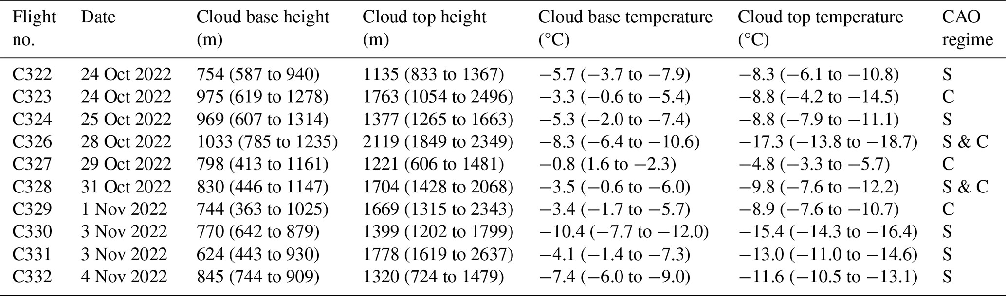
The M-Phase airborne campaign, described in detail by Clarke et al. (2026), took place in Autumn 2022, from 18 October to 5 November. Research flights targeting marine boundary layer cloud embedded within CAOs were conducted over the Labrador Sea in the North Atlantic Ocean, off the east coast of Canada (Fig. 1). The primary objective of M-Phase was to reduce uncertainties in (a) the mixed-phase cloud response to a warming climate, and (b) overall climate sensitivity. To achieve this, the FAAM (Facility for Airborne Atmospheric Measurements) BAe-146 (British Aerospace-146) aircraft was utilised to perform 15 research flights, each taking off and landing at Goose Bay (Fig. 1). The flight strategy incorporated a combination of sawtooth profiles (ascents and descents), predominantly through stratiform cloud regions, and straight-and-level (constant altitude) runs (SLRs) through convective cloud, when possible. Data recorded during the transit legs of each flight has been excluded here to avoid inclusion of high-altitude frontal cloud in the analysis. Each flight also included INP filter measurement legs, which took place at constant altitude upwind of cloud regions as well as above cloud top and below cloud base. Table 1 provides an overview of the cloud regions sampled during each flight which successfully captured north-westerly CAO flow, including cloud base and cloud top altitude and temperature (estimated from sawtooth profiles), and CAO regime (i.e. stratiform or convective). CAO flights were defined based on the marine CAO index (see Appendix B) and visual inspection of satellite imagery (Sect. 2.5); only data collected during CAO flights were included in our analysis.

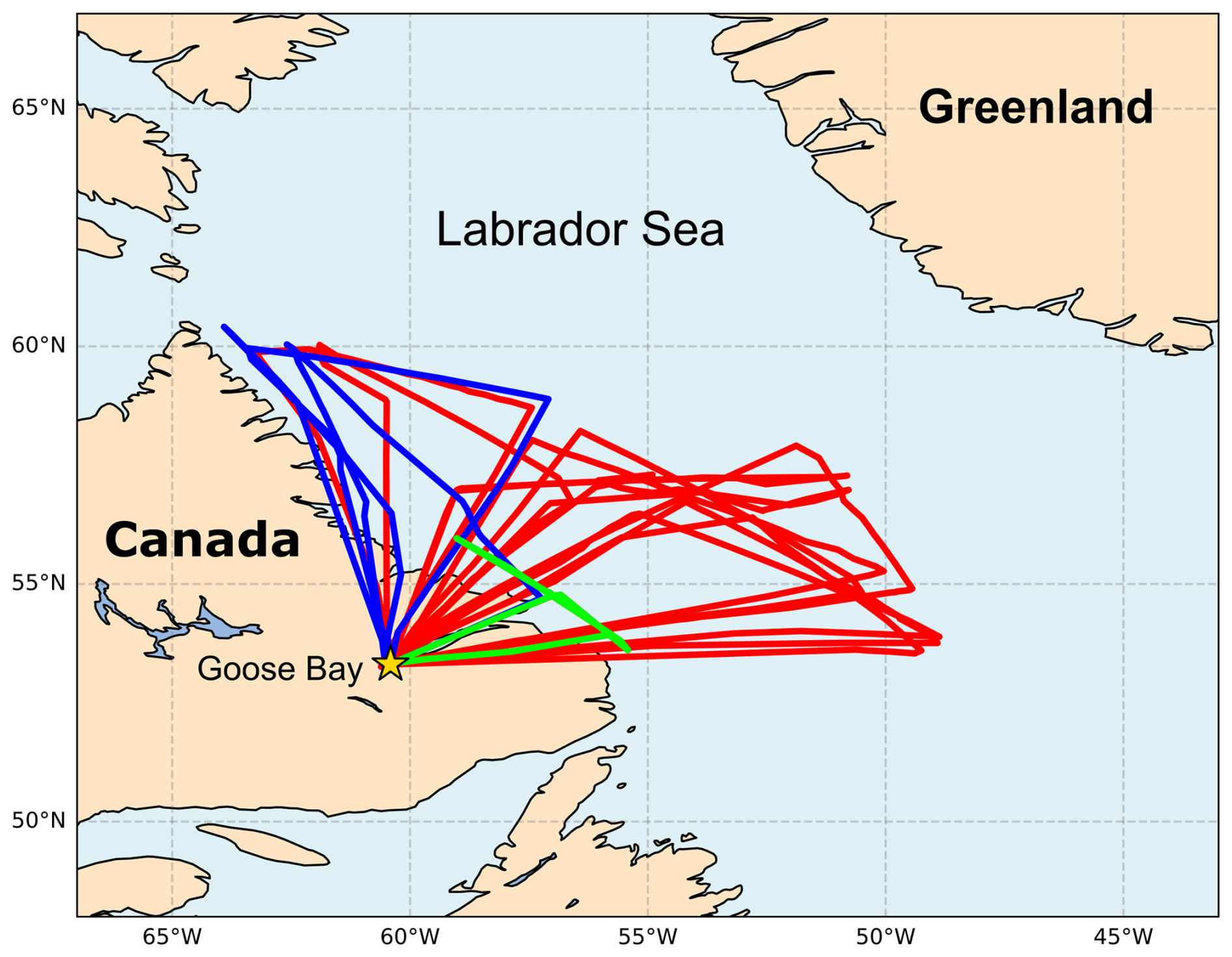
Figure 1 Labrador Sea with tracks from M-Phase flights C320 to C333 overlaid. The tracks of flights that captured north-westerly CAO flow are shown in red; those that sampled other airmasses and were excluded from the analysis are shown in blue. Flight C325, marked in green, targeted aerosol only. The location of Goose Bay is also marked (yellow star).

Table 1 List of M-Phase research flights considered in this study, including estimates of cloud base and top heights (m), and cloud base and top temperatures (°C). Values in bold denote mean values calculated from all sawtooth profile legs during each flight; minimum and maximum values are provided in brackets. Stratiform (S) or convective (C) CAO cloud regimes sampled by each flight are also provided.

In-situ measurements of cloud microphysical, aerosol and thermodynamic properties were made by a suite of instrumentation on-board the BAe-146 aircraft. A complete list and full description of all instruments operated during the campaign is given by Clarke et al. (2026). Here, we provide details of the instruments and associated measurements relevant for this study (Sect. 2.1–2.4). The separation of data into stratiform and convective cloud regimes is described in Sect. 2.5. Section 2.6 provides details of a splinter production rate calculation.

2.1 Ice crystal measurements

In this study, identification of SIP activity was based on in-situ measurements of total ice particle concentrations, analysis of the corresponding ice particles' shape and size, and comparisons with INP concentrations at the in-cloud temperature of observation derived from filter measurements. The following sections describe the main operating principles, uncertainties and processing steps associated with the optical array and imaging probes used during M-Phase for in-cloud ice crystal observations.

2.1.1 Two-Dimensional Stereoscopic Probe

The Two-Dimensional Stereoscopic probe (2D-S), manufactured by Stratton Park Engineering Company Inc. (SPEC), was the principal cloud instrument used for determining ice crystal size distributions during M-Phase. The 2D-S is an optical array probe (OAP) capable of providing information on the concentration, size and phase of cloud particles. The instrument comprises two identical orthogonal channels consisting of two laser beams that cross in the middle of the probe's sample volume (total of ∼ 16 L s⁻¹ at an airspeed of 100 m s⁻¹) and illuminate horizontally- and vertically-oriented 128-photodiode arrays. Shadows are produced on the arrays by particles of diameter (D_p) in the size range 10 to 1280 µm passing through either or both laser beams; images of these particles, with an effective pixel resolution of 10 µm, are built up over sequential time steps (Lawson et al., 2006). Note, particles were excluded from the analysis if their entire shadow was not contained within the photodiode array edges, thus reducing the effective sample volume for larger particles not meeting this requirement.

Raw data from the 2D-S probe was processed using the Optical Array Shadow Imaging Software (OASIS), developed by the National Centre for Atmospheric Science (NCAS) and Droplet Measurement Technologies (DMT) (Crosier et al., 2011). A threshold number of 10 µm pixels is set in the OASIS software, defining the minimum particle size accepted for further analysis. D_p describes a particle's maximum dimension length, therefore in this study, particles consisting of 20 pixels (i.e. a particle with D_p as small as 50 µm comprising 4 × 5 pixels) or less were initially excluded, given previously reported large uncertainties determining both the size (up to 50 %) and concentration (up to 100 %) of particles with D_p < 50 µm (Baumgardner and Korolev, 1997; Baumgardner et al., 2017). However, initial analysis of 2D-S particle size distributions for M-Phase revealed systematically high concentrations of ice between sizes of 50 and 100 µm across all flights, including those that captured strong evidence of recently active SIP processes (e.g. C328 and C329) and those showing negligible evidence of ice multiplication (e.g. C330 and C331) (Fig. A1 in Appendix A); this is consistent with results from early 2D-S testing by Lawson et al. (2006), in which measurements of particles of size less than 100 µm were found likely to be contaminated with out-of-focus liquid droplets erroneously identified as ice crystals. Therefore, for this work, further filtering of the 2D-S data was carried out, with only particles of D_p > 100 µm considered in the analysis; Baumgardner et al. (2017) reported reduced uncertainties of ∼ 20 % and ∼ 50 % for the size and concentration of ice crystals larger than 100 µm, decreasing further as particle size increases.

Further processing of the 2D-S data using the OASIS software included a correction for out-of-focus particles (Korolev, 2007) and application of an inter-arrival time algorithm, which removes particles with very short inter-arrival times indicative of ice crystal fragments potentially formed by shattering on the instrument (Field et al., 2006). Furthermore, following Crosier et al. (2011), discrimination was made between irregular and spherical particles based on geometric analysis of their circularity, C, according to Eq. (1):

$$\begin{array}{}\text{(1)}& C={\displaystyle \frac{P^{\mathrm{2}}}{\mathrm{4}\mathit{\pi }A}},\end{array}$$

where P is the particle perimeter and A is its area. Particle circularities were grouped into three categories: low irregular (LI), medium irregular (MI), and high irregular (HI). Particles with C < 1.2 are classified as LI; visual inspection of the corresponding 2D-S imagery confirmed that they were almost exclusively liquid droplets. Circularities greater than 1.4 are assigned to the HI category; from analysis of the particle imagery we concluded they were predominantly ice crystals. MI particles are defined as those with circularities between 1.2 and 1.4. Interpreting the phase of MI particles was a more complex task as the bulk of the images resembled aspherical ice crystals, often indicative of newly frozen drops; however, many poorly imaged liquid droplets were also likely defined as MI instead of LI. Moreover, the mean ratio of HI to MI particles during M-Phase was ∼ 10; therefore, even if, on average, some fraction of MI particles were ice crystals, the ice number concentration in the MI category would be substantially less than 10 % of the HI particle concentration. Thus, for this study, we assume the HI category alone is an accurate proxy for all ice crystals measured by the 2D-S probe. It should be noted that by (a) assuming all observed ice crystals were categorised as HI, and (b) excluding all particles with D_p < 100 µm, the ice crystal number concentrations reported in this study are likely to be slight underestimations of the true values.

In the past, measurements from aircraft-mounted cloud instruments have been subject to shattering artefacts as ice crystals collide with the probe tips (Heymsfield, 2007). For this flight campaign, the instrument was fitted with Korolev anti-shatter tips, or K-tips, designed to reduce particle-shattering artefacts by minimising inlet surface area and any inefficient heating that may cause ice to accumulate on the probe exterior (Korolev et al., 2013).

We use high time resolution 2D-S data (1 Hz); longer data averaging periods (e.g. 5 or 10 s) have previously been shown to provide a more statistically significant measurement (McFarquhar et al., 2007), but 1 Hz data enables us to better characterise fine-scale cloud structure and capture the expected large spatial variability in mixed-phase cloud ice and water contents (Huang et al., 2021; Wang et al., 2023). At an airspeed of 100 m s⁻¹, the minimum detectable ice concentration for each channel of the 2D-S is ∼ 0.12 L⁻¹ in a 1 s interval. Additionally, particle images can be captured at rates of up to 74 frames per second (Finney et al., 2024); therefore, the high sampling rate and spatial resolution of imagery measurable by the 2D-S enables the identification of cloud regions containing high concentrations of small ice crystals where SIP processes are most likely to be active (Lawson et al., 2006).

2.1.2 High Volume Precipitation Spectrometer

Larger ice crystals, including graupel and other precipitation-sized particles were identified in this study using the High Volume Precipitation Spectrometer Version 3 (HVPS-3, SPEC Inc.). The HVPS is a single array, two-dimensional shadow probe that functions similarly to the 2D-S, but its optics are configured to capture particle images at 150 µm resolution in the size range 150 µm < D_p < 19.2 mm. At an airspeed of 100 m s⁻¹, the sample volume is 310 L s⁻¹ (note, as with the 2D-S probe, sample volume is particle-size dependent), resulting in a minimal detectable ice concentration of ∼ 0.003 L⁻¹ at 1 Hz time resolution. Previous studies have found that ice fragments with D_p < 600 µm can be readily generated from larger crystals breaking up on impact with the HVPS probe arms, leading to the erroneous inclusion of small ice shattering artefacts in ice concentration measurements (Korolev and Isaac, 2005; Glienke and Mei, 2020; Wang et al., 2023); therefore, only particles observed by the HVPS with D_p > 600 µm were considered for this work.

Total ice concentrations were determined as the sum of HI particles observed by the 2D-S (100 < D_p < 1280 µm) and all particles measured by the HVPS outside of the particle size overlap with the 2D-S (D_p > 1280 µm); particles observed by the HVPS with D_p between 600 and 1280 µm were included if the number concentration was below the 2D-S detection limit (∼ 0.12 L⁻¹).

2.1.3 3 View-Cloud Particle Imager

High-resolution images of cloud hydrometeors were captured with the 3 View-Cloud Particle Imager (3V-CPI, SPEC Inc.), providing detailed information on in-cloud liquid-ice phase partitioning and enabling more refined ice crystal habit discrimination between active SIP and neighbouring aged, background ice regions. The 3V-CPI instrument comprises a 2D-S probe integrated with a Cloud Particle Imager (CPI, SPEC Inc.). The CPI is capable of imaging and counting liquid or ice particles (15 µm < D_p < 2500 µm) at a pixel resolution of 2.3 µm, with a sample volume of ∼ 0.37 L at an airspeed of 100 m s⁻¹ (Finney et al., 2024). Hydrometeors passing down its sample tube are captured via a three-laser system. Firstly, the 2D-S, operating as in the stand-alone instrument (Sect. 2.1.1), illuminates the particles that pass down the inlet tube on-axis through the sample volumes of its two orthogonal (continuous) laser beams, located in the laser crossover region, and the scattered light is projected onto two separate diode-array detectors. When a signal is recorded simultaneously by both detectors, an imaging laser is triggered, which illuminates the particles in the CPI sample area and the instrument's imaging optics focus this light onto a high-resolution 256 grey-scale fast CCD camera to record an image of the liquid droplet or ice crystal.

Analysis of the 2D-S shadowgraphs, alongside the higher resolution CPI imagery, enables detailed characterisation of ice crystal shapes and habits, thus assisting with understanding ice crystal generation and growth processes; this is critical for identifying active SIP mechanisms (Korolev and Leisner, 2020).

2.2 INP filter measurements

Each flight incorporated multiple upwind or below/above-cloud filter sampling legs, during which aerosol particles were collected onto polytetrafluoroethylene filters for offline analysis in a hotel room-based temporary laboratory to determine number concentrations of immersion freezing INPs (Price et al., 2018); ACAO, the sister campaign to M-Phase (Clarke et al., 2026), adopted the same filter sampling technique, which is described in detail by Raif et al. (2024). Filter samples were processed mostly within hours, but always within two days of collection, thus avoiding degradation of the samples associated with long-term storage and transport (Beall et al., 2020). Derived cumulative INP concentrations, providing a measure of expected cumulative primary ice particle numbers on cooling to a particular temperature, are directly compared with in-situ measurements of total ice concentrations from the same air mass to highlight potential SIP activity.

Constant-altitude filter legs typically lasted for 20–30 min; a total of 37 filter samples were collected during M-Phase, with at least two per flight to increase the spatial coverage and enable quasi-Lagrangian sampling for the cases where one sample was downwind from another. The droplet-on-filter, or drop-on, sampling technique was implemented for M-Phase and is detailed in Price et al. (2018) and Sanchez-Marroquin et al. (2019), with previous examples of its use in an Arctic environment reported by Sanchez-Marroquin et al. (2023). In brief, the drop-on technique involves placement of microlitre droplets of pure water onto an exposed filter atop a temperature-controlled stage that cools the array of droplets at a constant rate of 1 K min⁻¹. The fraction of droplets frozen at a particular temperature, along with the volume of air sampled during the corresponding filter leg, defines the cumulative INP concentration per litre of air for each filter sample (Price et al., 2018). Across all samples, the warmest temperature at which droplets froze, and INP concentrations were derived, was ∼ −9 °C; INPs at warmer temperatures were below the limit of detection (∼ 0.01 L⁻¹). Other offline filter-based INP measurements from a wide range of geographical locations were shown by Petters and Wright (2015) to decrease sharply (∼ 2 orders of magnitude) at higher temperatures (between −10 and −5 °C); therefore, if we assume a similar trend here, expected INP concentrations at the warmest in-cloud temperatures observed during M-Phase had likely maximum values of ∼ 10⁻⁴ L⁻¹. The coldest-temperature INPs were observed at ∼ −33 °C, with 100 % of droplets frozen at lower temperatures; however, observations at such cold temperatures were only possible in samples with relatively low INP concentrations, as all available droplets had already frozen at warmer temperatures for samples with higher INP concentrations.

2.3 Cloud water content and cloud droplet concentration measurements

The relative mass of supercooled liquid water and ice in mixed-phase clouds provides a measure of their level of glaciation, which, alongside ice number concentration and ice crystal habit, helps inform on whether SIP is occurring; if ice multiplication is at an early or late stage; and which SIP mechanisms are likely to be active.

Bulk liquid-water content (LWC), describing the mass of liquid water in a given volume of air, and total condensed-water content (TWC) (sum of liquid and ice) were measured in M-Phase using a Nevzorov hot-wire probe (Sky Physics Technology Inc.). The instrument's basic operating principle, described in detail by Korolev et al. (1998), incorporates a coiled wire component for LWC measurements and a separate deep cup TWC sensor; all elements are heated and operate at a constant temperature of 120 °C. Calculations of LWC and TWC are based on the power needed to compensate for heat losses following the evaporation of water or ice on contact with the heated probe elements (Korolev et al., 1998). Additional processing of the Nevzorov data was carried out by the UK Met Office, including a calculation of ice water content (IWC) based on the general assumption that the discrepancy between TWC and LWC measurements is solely due to ice particles (Abel et al., 2014); small corrections are applied to calculated IWC and measured LWC values in order to account for the residual signal from ice particles known to often be erroneously detected by the LWC sensor (Korolev et al., 1998; Evans et al., 2025).

The phase composition of sampled CAO cloud was determined here by calculating the ice mass fraction (μ₃) (Korolev et al., 2003), using measured total water content (W_total) and derived ice water content (W_ice) values, according to Eq. (2):

$$\begin{array}{}\text{(2)}& {\mathit{\mu }}_{\mathrm{3}}={\displaystyle \frac{W_{\mathrm{ice}}}{W_{\mathrm{total}}}}.\end{array}$$

Cloud regions with μ₃ < 0.1, 0.1 < μ₃ < 0.9, and μ₃ > 0.9 were classified as liquid, mixed-phase and glaciated (ice), respectively, following the threshold values applied by Korolev et al. (2003) and Evans et al. (2025).

In addition to the Nevzorov measurements of liquid water and total water content, cloud droplet concentrations and size distributions were obtained using the Cloud Droplet Probe (CDP, manufactured by DMT). The CDP measures forward-scattered light from an incident laser beam to detect cloud droplet particles ranging in diameter from 2–50 µm; cloud droplets are distributed across 30 size bins. Potential sources of uncertainty in the CDP measurement are discussed in detail in Lance et al. (2010) and include particle counting and sizing errors related to the non-monotonic relationship between droplet size and scattered light; coincidence occurring as multiple droplets pass through the probe's sample area in quick succession, so that one larger droplet is erroneously detected; and droplet shattering on contact with the instrument leading to the detection of more, smaller droplets. Overall, average droplet sizing and concentration uncertainties with the CDP are estimated to be ∼ 30 % and ∼ 20 %, respectively (Baumgardner et al., 2017).

For this study, the analysis is refined to only include data associated with in-cloud conditions (after removal of higher altitude frontal cloud sampled during transit legs) defined as a 1 Hz period with both: (a) Nevzorov TWC > 0.01 g m⁻³ (Korolev et al., 2003; Crawford et al., 2016; Huang et al., 2021), and (b) CDP total cloud droplet concentration > 1 cm⁻³. Application of the CDP threshold ensures that fully glaciated regions associated with below-cloud ice-phase precipitation, at temperatures around 0 °C, are removed from the analysis.

2.4 Thermodynamic data

Several other FAAM aircraft instruments were used to provide measurements of core thermodynamic variables. The ambient temperature was measured with a Rosemount type 102 probe (Price, 2022); vertical wind speed was provided by the Aircraft-Integrated Meteorological Measurement System (AIMMS-20) at 20 Hz resolution; and altitude was measured by the GPS-assisted Inertial Navigation system (GIN). We only considered vertical wind speeds measured during SLRs, or constant altitude flight legs, as determined by the GIN, to avoid using data contaminated by additional vertical airflow induced by upwards or downwards movement of the aircraft during sawtooth profiles (Beswick et al., 2008).

2.5 Separation of data into stratiform and convective regimes

In this study, we are particularly interested in exploring how SIP activity evolves moving downwind from stratus and stratocumulus cloud decks to broken, cumulus clouds in CAOs. To this end, we separated the cloud microphysical and thermodynamic data into stratiform and convective cloud regimes based on: (a) visual inspection of satellite imagery to identify the transition region from stratiform to cellular convective cloud, (b) review of aircraft-mounted video camera footage, and (c) discontinuities in the temporal variability of LWC and cloud droplet concentrations.

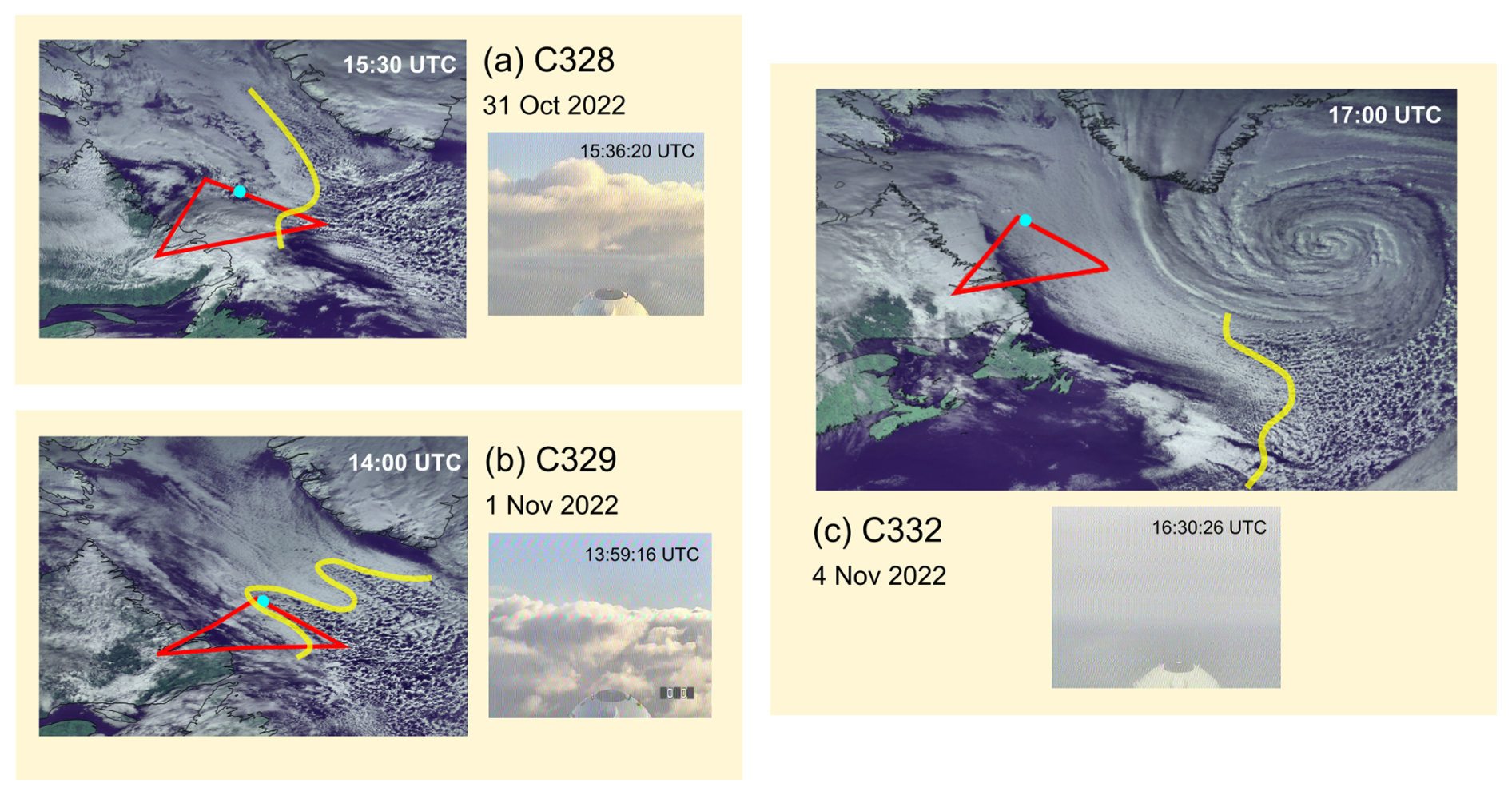
Figure 2 GOES-16 RGB composite satellite imagery, alongside images from the aircraft-mounted forward-facing camera, for M-Phase flights (a) C328, (b) C329, and (c) C332. Satellite overpass and camera image times are marked. Flight tracks are overlaid (red lines) and approximate locations of aircraft when camera image was captured are marked (blue circle). Yellow lines represent estimated location of stratiform-to-convective regime transition.

Figure 2 shows GOES-16 RGB composite satellite imagery, available every 10 min at 0.5 km resolution, and images from the forward-facing camera mounted on the BAe-146 aircraft from a selection of flights which sampled (a) both stratiform and convective CAO regimes (C328), (b) convective cloud only (C329), and (c) stratiform cloud only (C332). The flight tracks are overlaid on each satellite image and consist of a transit leg out over the Labrador Sea from Goose Bay, before the cloud sampling leg travelling south-east to follow the CAO flow, and a further transit leg back to Goose Bay. Flight C328 (Fig. 2a) initially sampled stratiform cloud utilising sawtooth profiles (Fig. 6a in Sect. 3.2), ascending and descending through the shallow cloud layer, reaching ∼ 150 m above and below cloud top and base; Fig. 2a shows a camera image taken shortly before the aircraft penetrated the stratocumulus cloud region. Flight C328 also captured the regime transition to convective cloud, marked by the yellow lines in Fig. 2; at an airspeed of 100 m s⁻¹, the aircraft covered the ground around five times faster than the cloud field and regime transition was migrating to the south-east, thus Flight C328 successfully captured the stratiform-to-convective cloud transition before reaching the end of the cloud sampling leg at approximately 16:35 UTC. Flight C329 (Fig. 2b) sampled convective cloud only, deploying a combination of sawtooth profiles and SLRs (Fig. 9a in Sect. 3.2); a camera image captured immediately before entering broken, cumulus cloud is shown in Fig. 2b. Figure 2c shows CAO cloud associated with the cold, dry sector of a mid-latitude cyclone with a low-pressure centre situated to the south-east of Greenland; Flight C332 took place entirely in the stratus cloud deck located approximately 1500 km upwind of the stratiform-to-convective regime transition region. Note, ambiguous cloud sections sampled during the flight campaign, where a clear distinction between stratiform and convective regimes was not possible, were excluded from the analysis.

2.6 Splinter production rate calculation

To quantitatively assess whether ice multiplication via the H–M process alone could be responsible for elevated ice concentration measurements, we have estimated the splinter production rate following the model developed by Willis and Hallett (1991), which was based on earlier work by Hallett et al. (1978), for cloud regions with temperatures falling within the active H–M range (−3 to −8 °C). If the calculated rate of ice splinter production is too slow to feasibly account for the observed ice crystal concentration enhancements, then other SIP mechanisms are likely to be active. From Hallett et al. (1978), rime splintering is estimated to produce new ice crystals at a rate according to Eq. (3):

$$\begin{array}{}\text{(3)}& {\displaystyle \frac{\mathrm{d}{N}_{\mathrm{ice}}}{\mathrm{d}t}}=\sum _{k=\mathrm{1}}^n{S}_k{N}_k,\end{array}$$

where N_k is the number concentration of graupel (or rimer) particles (1 Hz data) observed in graupel size bin k (n size bins in total); for this study, all measured ice crystals with D_p > 300 µm were assumed to act as rimers, following Järvinen et al. (2022). This rimer size threshold is consistent with previous analysis of micro-stereoscopic cloud particle images from the SOCRATES (Southern Ocean) and ACLOUD (Arctic) aircraft campaigns, conducted by Waitz et al. (2022), which determined that ice crystals of size 300 µm were twice as likely to have undergone significant riming as those smaller than 200 µm, with minimal increases in riming fraction at larger particle sizes. Furthermore, earlier experimental work showed that the minimum ice particle size for a non-zero droplet collection efficiency is around 300 µm for columns, hexagonal plates and broad-branched crystals (Kajikawa, 1974; Pitter, 1977; Wang and Ji, 2000). Here, each rimer is assumed to generate S_k ice splinters per unit time, calculated as:

$$\begin{array}{}\text{(4)}& S_k=N_{\mathrm{d}}\mathit{\alpha }\mathit{\pi }{D}_k^{\mathrm{2}}{V}_{\mathrm{g}}E/\mathrm{4},\end{array}$$

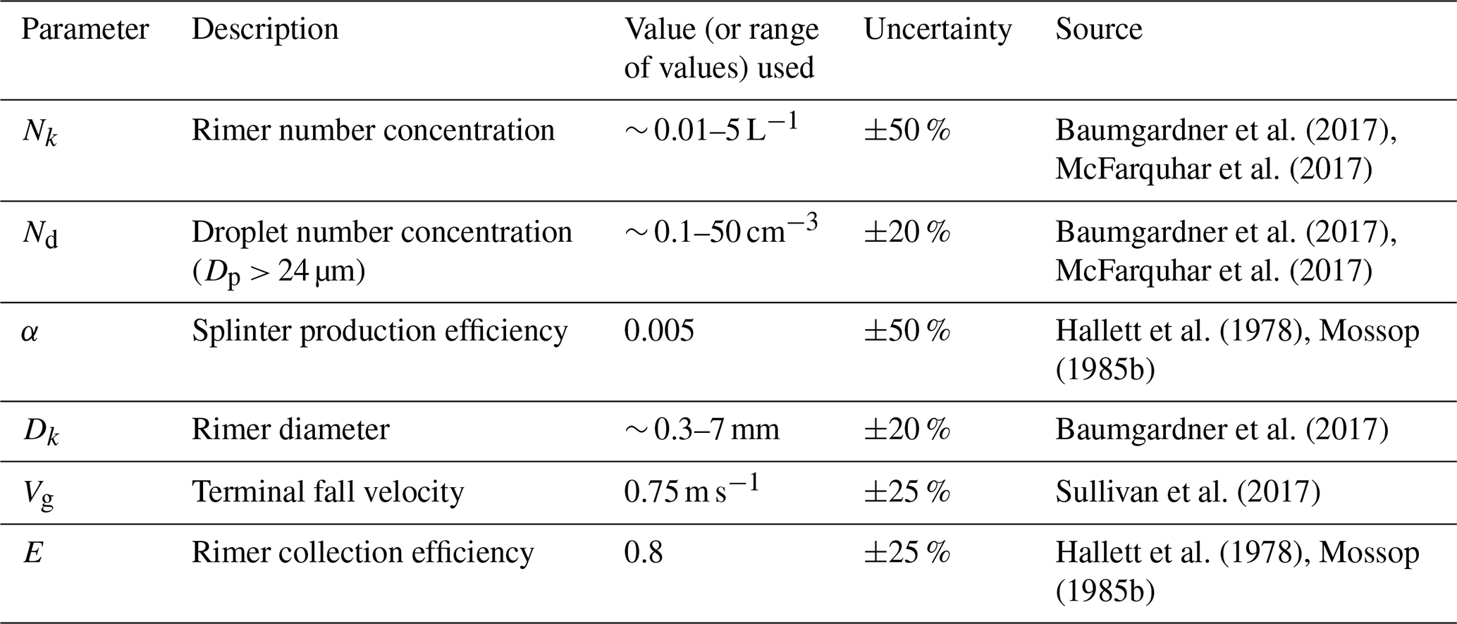
where the concentration of droplets with D_p > 24 µm is given by N_d; α is the splinter production efficiency, describing the average number of splinters produced for each rimer-droplet collision; D_k is the rimer diameter (midpoint of size bin k); V_g represents the rimer terminal fall velocity; and E is the rimer collection efficiency. To enable direct comparison between splinter production rates estimated for CAO clouds in the Northern and Southern Hemispheres, we assume the same values for α (0.005), V_g (0.75 m s⁻¹), and E (0.8) as used by Järvinen et al. (2022) for Southern Ocean clouds examined during the SOCRATES campaign. However, it is important to consider potential uncertainties in the splinter production rate calculation stemming from (a) measurement errors associated with cloud droplet and ice particle size distributions, and (b) rimer characteristic variability, which can impact the splintering parameters in Eq. (4) (i.e. α, V_g, and E) depending on the dominant rimer particle type and size within a particular cloud segment; for instance, large graupel particles will fall through a cloud at a greater velocity than more recently generated columnar crystals, directly impacting riming efficiency and splinter production (Mossop, 1985b). Table 2 summarises the uncertainties associated with each input parameter in Eq. (4) according to previously published analyses of CDP and OAP measurement uncertainties (Baumgardner et al., 2017; McFarquhar et al., 2017), and results from early rime splintering laboratory studies (Hallett and Mossop, 1974; Mossop, 1985b). Based on the propagation of errors in Eq. (4), we estimate a typical uncertainty of ±86 % in calculated splinter production rates.

Table 2 Uncertainties (%) in each parameter used in the splinter production rate calculation.

3 Results and Discussion

First, we provide an overview of the cloud microphysical data collected during the M-Phase campaign and discuss initial evidence of ice multiplication across stratiform and convective CAO cloud regimes (Sect. 3.1). Section 3.2 presents a comprehensive analysis of specific SIP mechanisms which may be active and responsible for the observed ice concentration enhancements. In Sect. 3.3, a summary of the most favourable environmental conditions for activating SIP processes during M-Phase is presented.

3.1 Ice particle concentrations and evidence of SIP in stratiform and convective regimes

Comparisons between in-situ ice concentration and INP measurements provide information on active in-cloud ice formation processes. Similar magnitude ice crystal and INP concentrations measured at the same temperature suggest primary ice production is dominant, whereas much greater ice compared to INP concentrations are indicative of active ice multiplication processes. Figure 3a shows total ice crystal number concentrations (N_ice) measured at 1 Hz resolution with the 2D-S and HVPS probes, and INP concentrations (N_INP) derived from filter measurements as a function of in-cloud temperature for all CAO flights (Table 1) during the M-Phase campaign. The largest 1 Hz N_ice values were observed at ∼ −8 °C, frequently exceeding 100 L⁻¹ and reaching a maximum of 488 L⁻¹. Similar magnitude peak ice concentrations have been observed around this temperature in shallow, mixed-phase clouds during previous airborne campaigns across the Northern Hemisphere (McFarquhar et al., 2007; Crawford et al., 2012; Wang et al., 2023).

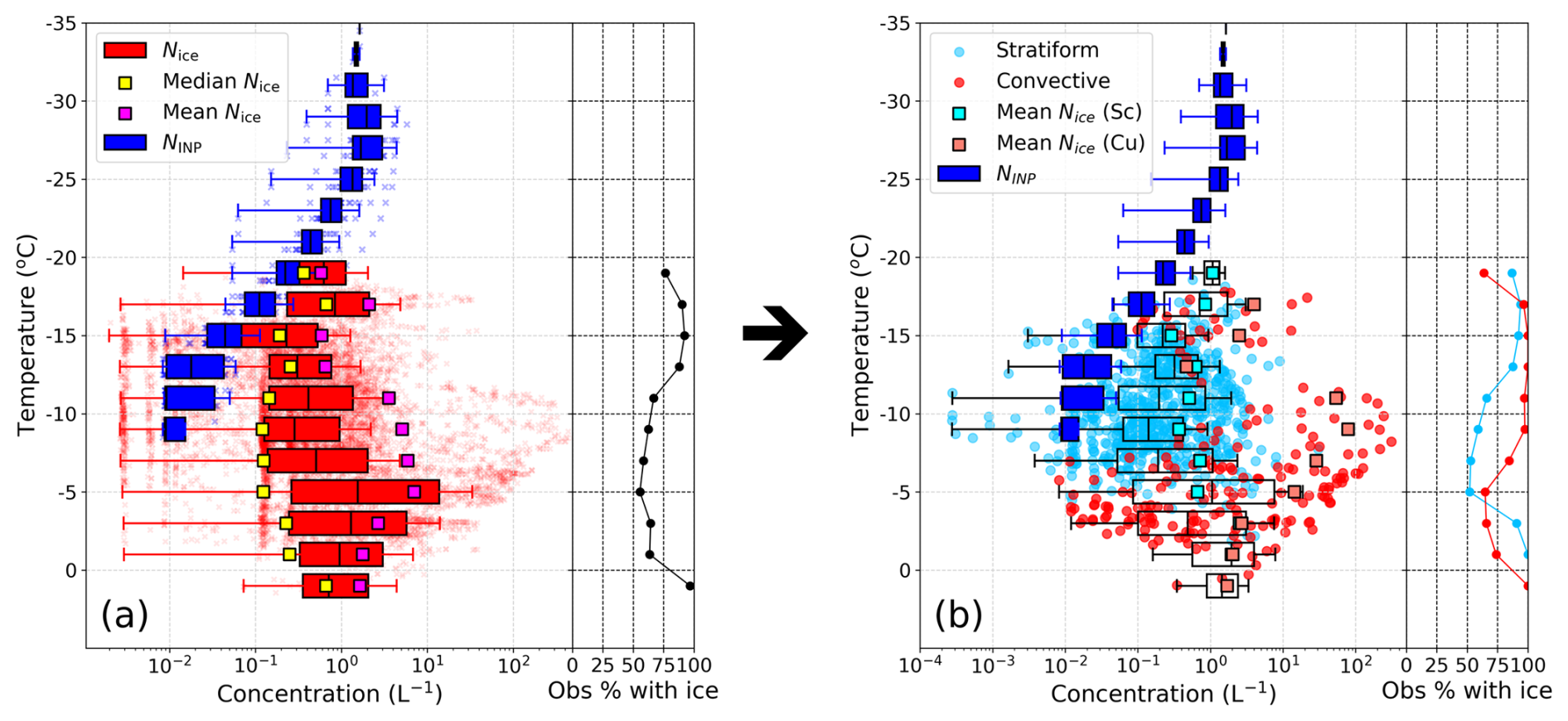
Figure 3 (a) Measured total (2D-S + HVPS) ice crystal number concentrations (N_ice; red) as a function of local in-cloud temperature (1 Hz data) for all CAO flights during M-Phase; only data above the instrument detection limit (i.e. non-zero ice concentrations) are displayed. Boxplots (red) for N_ice above the instrument detection limit in 2 °C temperature bins are composed of centre lines, edges and whiskers representing the median, interquartile range (25th to 75th percentile) and nearest data points within 1.5 × interquartile range of the lower and upper quartiles, respectively. Median N_ice (yellow squares) and mean N_ice (pink squares) are calculated from all data points, including N_ice below the instrument detection limit (i.e. where we have set N_ice to 0 L⁻¹). The percentage of in-cloud data containing detectable ice within each temperature bin is also provided (black line). Measured INP concentrations (N_INP) derived from all filter samples collected during CAO flights are shown in blue. (b) N_iceseparated into 10 s averaged regions within individual stratiform (Sc; light blue) and convective (Cu; red) cloud segments; mean N_ice and percentage of ice concentration observations (1 Hz data) above 0 L⁻¹, as shown in panel (a), are also separated by CAO regime. Boxplots represent 10 s averaged data from both CAO regimes.

Mean N_ice, calculated including cloud regions where measured ice crystal concentrations were below the instrument detection limit (i.e. we set N_ice = 0 L⁻¹), peaked at 7.1 L⁻¹ between −4 and −6 °C (Fig. 3a); however, 44 % of ice concentration measurements within this temperature range contained no detectable ice, the highest proportion across all in-cloud temperatures observed during the campaign. Järvinen et al. (2022) also reported the highest mean N_ice at ∼ −5 °C (9.8 L⁻¹) in Antarctic summertime marine CAO clouds examined during the SOCRATES campaign, including a similar fraction of data below the instrument detection limit (∼ 40 %). When pockets of high ice concentrations, up to four orders of magnitude greater than expected N_INP (Fig. 3a), are frequently observed at the same temperature as liquid-dominated cloud regions containing negligible or very low amounts of ice, it is likely SIP processes are active but only initiated when particular environmental thresholds are met; specifically, the rime splintering mechanism may have regularly been triggered during M-Phase, given peak ice concentrations were generally measured within the active H–M range (−3 to −8 °C).

A secondary peak in measured ice particle concentrations was observed at ∼ −17 °C during M-Phase (Fig. 3a); N_ice values reached up to 34 L⁻¹ with a median of 0.9 L⁻¹ between −16 and −18 °C, an order of magnitude above the corresponding median N_INP (∼ 0.1 L⁻¹). Several previous in-situ measurement studies have reported similar ice crystal enhancements within this colder temperature region in mixed-phase clouds (Yang et al., 2014; Mignani et al., 2019; Järvinen et al., 2022); ice multiplication in these cases was attributed to ice-ice collisional breakup based on ice crystal image analysis and the results of earlier ice break-up laboratory experiments (Vardiman, 1978; Takahashi et al., 1995; Grzegorczyk et al., 2023).

Table 3 Summary of sampled stratiform and convective cloud segments (cloud segment defined where ≥ 5 consecutive seconds of in-cloud conditions were sampled), including mean in-cloud temperature, mean (and 95th percentile) ice crystal number concentration (N_ice), and mean (and 95th percentile) ice mass fraction (μ₃); all calculated from 1 Hz data.

To explore how SIP may evolve downwind in CAOs, as stratocumulus cloud decks break up into cumulus clouds, we separated the 1 Hz N_ice data into 10 s averaged regions contained within individual cloud segments belonging to either the stratiform or convective CAO regimes (Fig. 3b), as described in Sect. 2.5; we condensed the N_icedata from 1 to 0.1 Hz resolution in Fig. 3b to more clearly isolate any regime-specific trends in ice number concentration and thus potential SIP activity. Here, a cloud segment is defined as a period during which a minimum of 5 consecutive seconds of in-cloud conditions (TWC > 0.01 g m⁻³ and cloud droplet concentration > 1 cm⁻³) were sampled. Following these criteria, 215 stratiform and 132 convective cloud segments were identified during CAO flights in M-Phase (Table 3). On average, sampling within individual stratiform and convective cloud segments lasted for 37 and 18 s, respectively, with maximum durations of 224 s in stratiform and 100 s in convective cloud. This discrepancy in sampling duration, and hence cloud segment spatial coverage, reflects the breakup of expansive stratiform cloud into cellular cumulus clouds as sea surface temperatures and turbulent heat fluxes increase with distance south in the Labrador Sea.

On average, lower temperatures were observed in stratiform (−10.2 °C) compared to convective cloud (−6.2 °C), which is reflective of the sampling strategy; sawtooth profiles ascended to cloud top within stratiform cloud, whereas SLRs often targeted lower altitudes within convective cloud due to both challenges operating the aircraft in highly turbulent conditions and the increased risk of aircraft icing at higher in-cloud altitudes. Mean ice particle concentrations measured in convective cloud (16.2 L⁻¹) were more than an order of magnitude greater than in stratiform cloud (0.5 L⁻¹). Moreover, 25 % of cumulus cloud regions (10 s averaged) had ice concentrations greater than 10 L⁻¹, a strong indicator of SIP activity given INP concentrations were at least an order of magnitude below this at all cloud top temperatures during M-Phase; maximum N_INP at the coldest cloud top temperature (−18.7 °C during flight C326) was ∼ 1 L⁻¹, as shown in Fig. 3a. Of these well-glaciated, cumulus cloud regions, 69 % had temperatures within the H–M zone (Fig. 3b). The mean μ₃ value (and 95th percentile) in the convective regime was 0.24 (0.88), compared to 0.06 (0.46) in the stratiform regime (Table 3), further illustrating the extent to which cloud glaciation levels increased across the regime transition.

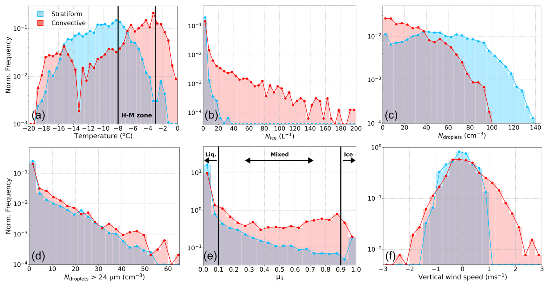
Figure 4 Relative frequency histograms of cloud microphysical properties (1 Hz data) measured within the stratiform (blue) and convective (red) regimes during all M-Phase CAO flights, including (a) local in-cloud temperature (H–M zone marked), (b) ice crystal number concentration (N_ice), (c) total cloud droplet concentration (N_droplets), (d) concentration of cloud droplets with diameter > 24 µm, (e) ice mass fraction (μ₃) with thresholds for liquid, mixed and ice phase cloud regions marked, and (f) vertical wind speed (straight-and-level runs only). Data is normalised so that area under both stratiform and convective histograms integrates to 1.

Figure 4 summarises measurements of key microphysical properties (1 Hz data) made within stratiform and convective cloud during M-Phase. Relative frequency histograms of in-cloud temperatures observed in both CAO regimes (Fig. 4a) show that a greater proportion of measurements were made within the active H–M temperature zone in convective (61 %) versus stratiform (34 %) cloud. Sampling biases at warmer temperatures more conducive to SIP activity may have contributed to the substantial differences in glaciation observed in both regimes. However, if sampling bias was the primary factor driving observed glaciation differences, we would still expect to see some instances of comparable magnitude peak N_ice within the H–M temperature range in both regimes when other local environmental conditions were favourable for SIP, but this was not the case during M-Phase; ice particle concentrations above ∼ 40 L⁻¹ were measured in convective cloud only (Fig. 4b), with mean N_ice values of 0.6 and 15.1 L⁻¹, between −3 and −8 °C, in the stratiform and convective regime, respectively. Future airborne campaigns in CAO cloud systems would benefit greatly from more frequently targeting non-rime splintering temperature zones, such as between −15 and −18 °C, where a secondary peak in N_ice was detected in cumulus cloud regions during M-Phase; only ∼ 11 % of measurements in the convective regime were made within this colder temperature zone.

The highest total cloud droplet concentrations, reaching ∼ 140 cm⁻³, were observed in stratiform cloud; cloud droplet concentrations in convective regions did not exceed ∼ 100 cm⁻³ (Fig. 4c). Lloyd et al. (2018) reported cloud droplet concentrations of comparable magnitude in liquid-dominated stratocumulus clouds in wintertime CAOs over the North Atlantic, which decreased by a similar amount across the regime transition into broken, convective cloud. However, also in agreement with Lloyd et al. (2018), the highest concentrations of supercooled liquid drops with a diameter greater than 24 µm, considered to be a requirement for the H–M process (Mossop, 1978), were more frequently observed in cumulus relative to stratus or stratocumulus cloud regions (Fig. 4d). This increase in cloud droplet size with distance downwind in CAOs has previously been attributed to enhanced collision coalescence under more convective conditions generating more precipitation-sized droplets which, in turn, can lead to more efficient aerosol removal, inhibiting the formation of new cloud droplets (Abel et al., 2017; Murray-Watson et al., 2023).

Stratus and stratocumulus cloud regions sampled throughout the campaign were dominated by supercooled liquid water, illustrated by Fig. 4e, which shows that 86 % of μ₃ values in the stratiform regime were below 0.1 (i.e. liquid phase); a significant proportion of sampled cumulus clouds were also liquid phase (56 %). McFarquhar et al. (2007) and Huang et al. (2021) similarly found that single layer stratocumulus and shallow convective clouds were mostly liquid phase during intensive aircraft campaigns over the Arctic and Southern Oceans, respectively. However, during M-Phase, greater levels of in-cloud glaciation were observed much more frequently in the convective regime; μ₃ values above 0.5 were determined for 23 % and 0.5 % of measurements in convective and stratiform cloud, respectively. This is evidence that, when ice was present, the conditions necessary for the initiation of SIP were more regularly experienced in the convective CAO regime. Specifically, it is well-documented that, in mixed-phase conditions at warmer temperatures (within active H–M range), the large liquid drops detected in shallow convective cloud (Fig. 4d) can readily interact with preexisting ice particles within convective updrafts to initiate ice multiplication (Mason, 1996; Huang et al., 2017; Sullivan et al., 2017; Wang et al., 2023).

During the M-Phase campaign, the strongest downdrafts and updrafts, between ±1 and 3 m s⁻¹, were exclusively observed in convective cloud regions (Fig. 4f). Moderately strong updrafts (+1 to 3 m s⁻¹), comprising 14 % of measurements in the convective regime, are particularly well-known to stimulate SIP by generating sufficient supersaturation to form and grow large hydrometeors, and then by lofting them to the optimal temperature zones for ice multiplication (Sullivan et al., 2018). The consumption of liquid droplets within updrafts through microphysical processes such as riming and the WBF process, leading to ice crystal growth and SIP, can produce fully glaciated cloud regions (μ₃ > 0.9) (Fig. 4e); this was also reported by O'Shea et al. (2017) for shallow layer mixed-phase clouds over coastal Antarctic regions during the Microphysics of Antarctic Clouds (MAC) field campaign.

To help verify whether the stratiform-convective cloud contrast was a real regime effect and not driven by temperature-sampling biases, we repeated the analysis from Fig. 4, but for flights C322 and C323 only (vertical wind speed excluded as flights consisted solely of sawtooth profiles) (Fig. C1 in Appendix C). These flights sampled the stratiform (C322) and convective (C323) regimes of the same CAO event on the same day, enabling a more direct regime comparison. Both flights sampled the same air mass, with cloud top temperatures remaining relatively consistent throughout (Table 1), and observations were predominantly made within the H–M temperature range, with 68 % (692 s) and 85 % (611 s) of in-cloud measurements taking place between −3 and −8 °C during C322 and C323, respectively. Ultimately, the relative frequency histograms shown in Fig. C1 for both flights, which only include data recorded at temperatures within the H–M range to further eradicate any potential sampling bias effects, mirror the key stratiform-convective regime differences shown for the full campaign in Fig. 4; cumulus cloud regions generally comprised higher concentrations of large liquid droplets (D_p > 24 µm) but were substantially more glaciated than the stratiform cloud layer sampled upwind of the regime transition.

Overall, the results presented in Fig. 4 indicate that the microphysical and thermodynamic properties of cumulus clouds embedded in the convective regime of CAOs are more conducive to initiating SIP than those in the stratiform regime. Specifically, ice multiplication seemed to favour specific temperature zones (H–M range and ∼ −15 to −18 °C) that coincided with a strong supply of large, supercooled liquid drops (D_p > 24 µm) and moderate updrafts.

3.2 Analysis of active SIP mechanisms

Improvements to model parameterisations of ice multiplication processes, needed to reduce uncertainties in the mixed-phase cloud response to a warming climate, require better understanding of the underlying physics, bulk effects and environmental conditions favourable for specific SIP mechanisms (Qu et al., 2022). In this section, we present in-situ observations of cloud microphysical properties and high-resolution ice crystal imagery within distinct periods of SIP activity sampled during M-Phase to help understand the key markers and effects of the dominant SIP mechanisms active within CAOs.

3.2.1 Evidence of rime splintering

In Sect. 3.1, we showed that peak ice crystal number concentrations during M-Phase, exceeding expected INP concentrations at the same temperature by more than four orders of magnitude, were observed in the active temperature range for the H–M process. These well-glaciated cloud regions were found predominantly in the convective CAO regime, which was characterised by a high frequency of moderate updrafts and a strong supply of large, supercooled liquid droplets; such conditions have been determined by previous airborne studies to be conducive to the H–M process in shallow, mixed-phase clouds (Hou et al., 2021; Huang et al., 2021).

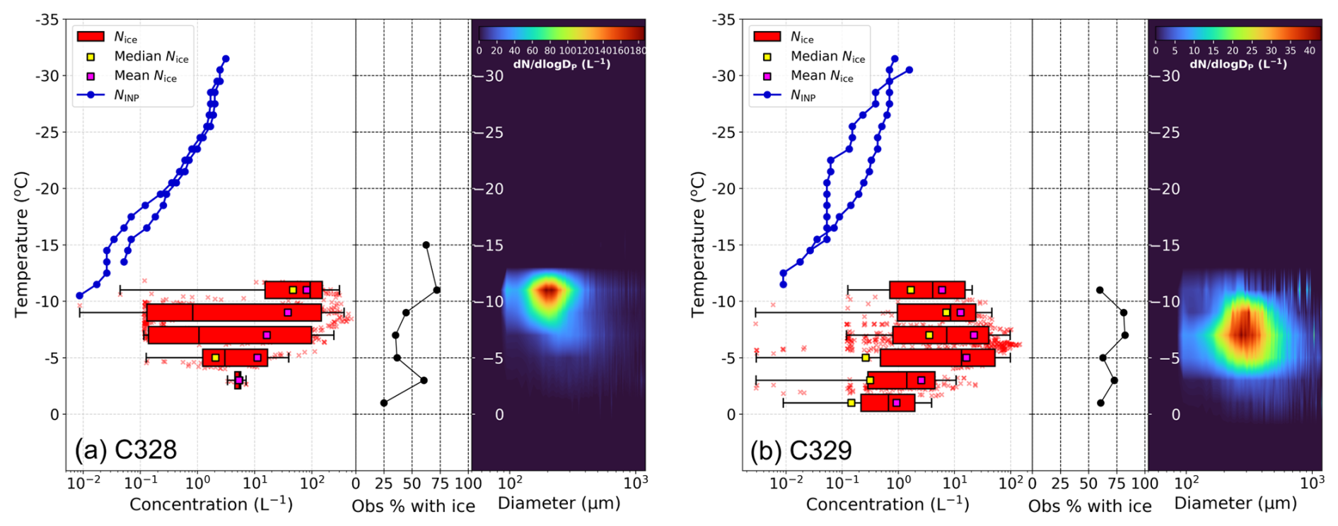
Figure 5 Measured total (2D-S + HVPS) ice crystal number concentrations (N_ice; red) as a function of local in-cloud temperature (1 Hz data) for flights (a) C328 (31 October 2022), and (b) C329 (1 November 2022). Boxplots (red) for N_ice above the instrument detection limit in 2 °C temperature bins are composed of centre lines, edges and whiskers representing the median, interquartile range (25th to 75th percentile) and nearest data points within 1.5 × interquartile range of the lower and upper quartiles, respectively. Median N_ice (yellow squares) and mean N_ice (pink squares) are calculated from all data points, including N_ice below the instrument detection limit (i.e. where we have set N_ice to 0 L⁻¹). The percentage of ice concentration observations above 0 L⁻¹ within each temperature bin is also provided (black line). Measured INP concentrations (N_INP) derived from filter samples collected during both flights are shown in blue. Mean ice particle size distributions as a function of local in-cloud temperature for both flights are presented in the right panel of panels (a) and (b).

Figures 5 to 11 focus on flights C328 and C329, which took place on 31 October and 1 November 2022, respectively. Both flights sampled convective cloud regions of CAOs (C328 sampled the stratiform-to-convective regime transition) at relatively warm temperatures, within the active H–M range, and measured the highest N_ice during the campaign (Fig. 5). The ice particle size distribution (PSD) during C328 peaked between −9 and −11 °C across a narrow diameter range between 150 and 300 µm (Fig. 5a); high concentrations of small ice particles were frequently observed at temperatures a few degrees below the H–M range during the campaign and are likely related to secondary ice particles formed at lower in-cloud altitudes that have mixed upwards in convective updrafts to the point of observation. A broader size distribution peak was observed during C329, between 200 and 500 µm (Fig. 5b), at slightly warmer in-cloud temperatures (∼ −6 to −9 °C). The larger ice crystals observed during C329 may have been generated in an older SIP cell elsewhere in the cloud, before growing and evolving whilst travelling to the measurement point via advection or turbulent mixing, or by precipitating down from a higher altitude. Results from early laboratory-based work (Ryan et al., 1976) and more recent innovative cloud seeding experiments (Fuchs et al., 2025) investigating depositional ice crystal growth rates in mixed-phase clouds indicate that at temperatures within the active H–M range, assuming linear growth over time, newly generated ice columns will grow to lengths exceeding 200 µm in around 5 min (at ∼ −5 °C) to 15 min (at ∼ −8 °C). This growth time is comparable with the convective overturning timescale in these CAO clouds; at an updraft speed of ∼ 1 m s⁻¹, air would mix over a cloud depth of ∼ 1 km in around 15 min. Therefore, some of the ice crystals observed near cloud top during C329, for example, may have formed closer to cloud base under slightly different environmental conditions, limiting how confidently we can directly link all ice production to the conditions at the point of observation.

3.2.2 Case study 1 – Flight C328 on 31 October 2022

Time series of selected cloud microphysical properties (10 s averages) measured during flight C328 are shown in Fig. 6; 10 s averages are shown here to reduce the noise present in the 1 Hz data, so that in-cloud features are more clearly visible. Stratiform cloud was sampled from approximately 15:24 to 16:15 UTC; however, this was initially non-continuous, partially broken cloud (until ∼ 15:51 UTC), likely not part of the main north-westerly CAO flow, as evidenced by the satellite imagery in Fig. 2a. Cloud droplet number concentrations and LWC values measured during the sawtooth profiles conducted between 15:51 and 16:15 UTC were relatively consistent, peaking at ∼ 30–50 cm⁻³ and ∼ 0.2–0.4 g m⁻³, respectively, upon each entry into the shallow stratus cloud layer (Fig. 6). After the regime transition into broken convective cloud (16:15 to 16:35 UTC), cloud droplet concentrations decreased and glaciation levels increased significantly, with mean μ₃ values reaching ∼ 0.7 in each sampled cumulus cloud segment (Fig. 6d).

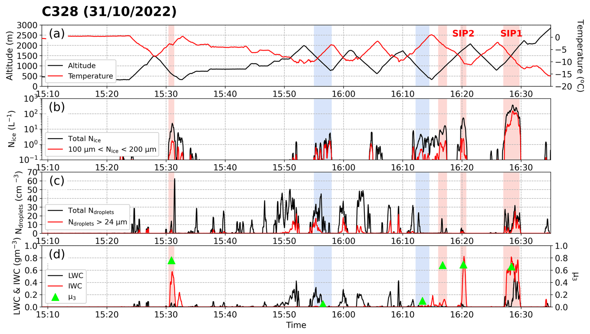
Figure 6 Time series of cloud microphysical properties (10 s averages) measured during flight C328 on 31 October 2022 (transit leg data excluded), including (a) temperature (red line) and altitude (black line), (b) total ice crystal number concentration (N_ice; black line) and concentration of ice particles with diameter > 100 and < 200 µm (red line), (c) total cloud droplet concentration (N_droplets; black line) and concentration of cloud droplets with diameter > 24 µm (red line), and (d) liquid water content (LWC) and ice water content (IWC). SIP and background ice regions are shaded in red and blue, respectively. Mean ice mass fraction (μ₃) values for SIP and background ice periods are also marked in panel (d) (green triangles).

Periods of active, or recently active, SIP processes (red-shaded regions in Fig. 6) were inferred from episodes of elevated ice concentrations that coincided with clear evidence of ice crystal fragmentation or splintering from manual inspection of 2D-S and CPI imagery. Neighbouring regions of lower “background” ice concentrations, where the ice particle imagery contained minimal evidence of SIP activity, are shaded in blue; although SIP does not appear to be active in these regions, measured background ice concentrations were still well above the N_INP at the relevant local cloud temperature and therefore likely contain some amount of aged secondary ice, originating elsewhere in the cloud, or primary particles that have sedimented down from near cloud top. Alternatively, background ice concentrations that exceed expected N_INP could be driven by some degree of spatial inhomogeneity in the INP population within the same air mass of a particular CAO event; however, it's important to note that throughout the entire campaign, N_INP at any given in-cloud temperature varies by less than an order of magnitude across all upwind and below/above-cloud filter measurement legs during CAO flights (Fig. 3). As such, it is highly unlikely that spatial variability in aerosol source, and thus N_INP, rather than ice multiplication processes, was the primary driver of N_ice variability of up to 2–3 orders of magnitude during SIP periods (Fig. 6).

During C328, N_ice across SIP regions varied from 2.0 L⁻¹ (5th percentile) to 324.9 L⁻¹ (95th percentile), with a mean of 110.7 L⁻¹. In contrast, ice particle concentrations measured across adjacent background regions were ∼ 1–2 orders of magnitude lower. As N_ice was above the corresponding N_INP at all temperatures (where INP measurements were above the detection limit) during C328 (Fig. 5a), secondary ice was likely mixed throughout the full sampled cloud region; our aim here was to establish the in-cloud properties (e.g. temperature, cloud droplet concentration or ice mass fraction) characterising the identified SIP periods (Fig. 6) in order to understand why ice multiplication had more recently initiated here versus nearby background regions.

SIP period 1 (hereafter, SIP 1), between 16:27:00 and 16:29:45 UTC, is marked in Fig. 6 and spanned the full vertical extent of a sampled cumulus cloud segment with cloud base and cloud top heights of ∼ 1100 and ∼ 2075 m, respectively; the corresponding cloud base and top temperatures were ∼ −4.5 and ∼ −12.2 °C, respectively. SIP 1 contained the highest measured ice concentrations across all SIP periods sampled during M-Phase, with a mean value of 154.3 L⁻¹ (1 Hz data); 40 % of the ice particles detected during this period had a diameter of less than 200 µm, suggesting ice multiplication processes were recently active. The mean in-cloud temperature during SIP 1 was −8.5 °C (∼ 40 % of measured temperatures were within the H–M zone) and conditions were mixed-phase ($\stackrel{\mathrm{‾}}{{\mathit{\mu }}_{\mathrm{3}}}$ = 0.66), with a strong supply of supercooled liquid droplets of diameter greater than 24 µm (${\stackrel{\mathrm{‾}}{N}}_{\mathrm{droplets}>\mathrm{24}\mathrm{\mu }\mathrm{m}}$ = 8.5 cm⁻³); therefore, the environmental conditions were favourable for the H–M process to occur.

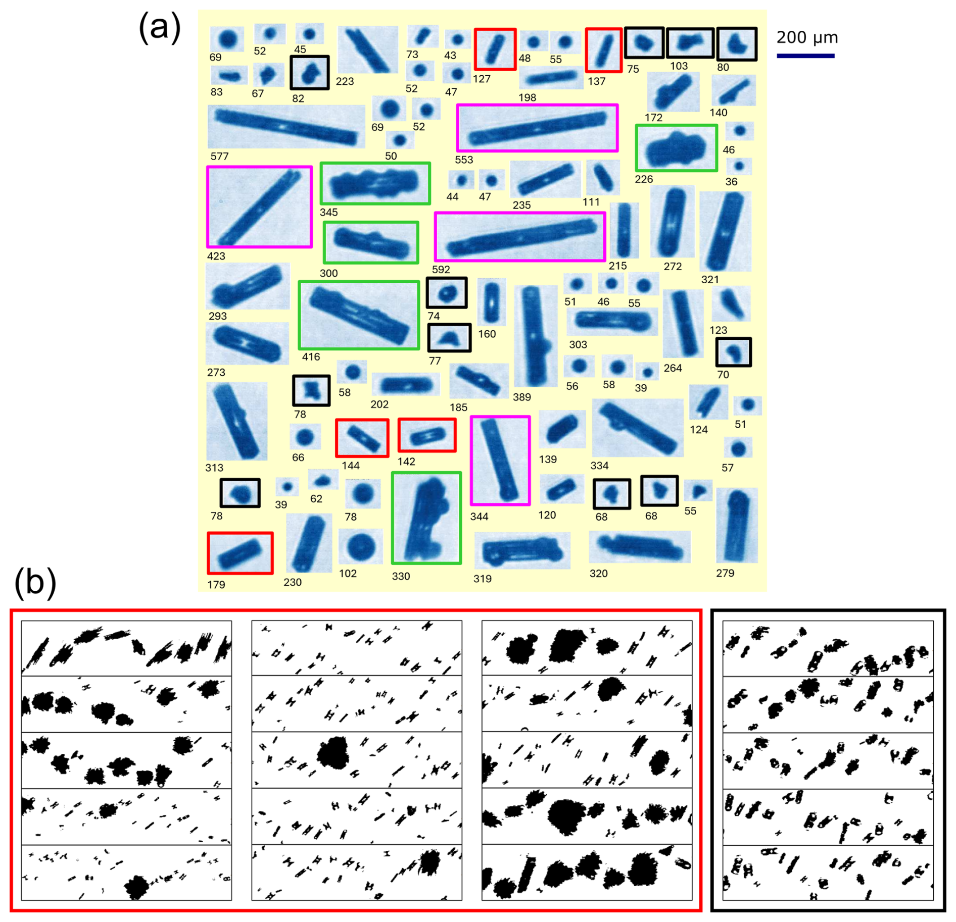
Figure 7 (a) Examples of cloud particles (ice crystals and liquid droplets) imaged with the CPI probe in SIP period 1 (between 16:27:00 and 16:29:45 UTC) during flight C328 (31 October 2022); subsets of small columnar ice of size < 200 µm (red frames), long columns (pink frames), rimed columns (green frames), and possible frozen droplets and fragments of shattered droplets (black frames) are highlighted; numbers below images indicate the maximum dimension length (D_p) of each particle. (b) 2D-S images of highly irregular particles captured in SIP 1; the height of each strip corresponds to the 2D-S array width of 1280 µm.

Figure 7a shows a sequence of CPI images of cloud particles (liquid droplets and ice crystals) from SIP 1. Ice particles observed within this cloud segment were predominantly small, faceted columns of length between 100 and 200 µm (red frames). The local in-cloud temperature during SIP 1 was within the range for columnar growth (∼ −4 to −10 °C), therefore these small ice crystals likely originated via SIP processes nearby, before growing by vapour deposition whilst in transit to the measurement location. Aged ice particles observed during this period were mainly longer columns or needles (300 µm < D_p < 600 µm) (pink frames), some of which had undergone visible riming (green frames). This riming was facilitated by the high concentrations of supercooled liquid droplets present during SIP 1 (${\stackrel{\mathrm{‾}}{N}}_{\mathrm{droplets}}$ = 17.2 cm⁻³), with those of diameter greater than 24 µm comprising nearly half of all droplets observed throughout this period (Fig. 7c); a few larger, drizzle-sized drops with D_p > 100 µm were captured by the CPI probe and are shown in Fig. 7a. The 2D-S imagery (Fig. 7b) captured during SIP 1 shows rapid transitions in ice crystal morphology between large, heavily rimed particles or graupel and regions dominated by small columns or splinters (red frame), consistent with the activation of the H–M process.

A small subset of the CPI images of droplets from SIP 1 have distorted shapes with bulges (black frames) indicating they had frozen or were undergoing freezing at the time of observation (Korolev et al., 2020). Some of these images have small spicule-like regions protruding from the frozen droplet surface, indicative of jetting following the build-up of internal pressure and subsequent cracking of the droplet's freezing outer shell (Lauber et al., 2018); sharp fragments of shattered frozen drops are also highlighted in Fig. 7a (black frames). Examples of frozen droplets, some with adjacent shattered fragments, were also captured by the 2D-S (Fig. 7b; black frame).

In summary, the cloud microphysical properties, environmental conditions and ice crystal habits observed during SIP 1 are consistent with those expected for active rime splintering; however, it is possible that other mechanisms, such as the fragmentation of freezing droplets, were acting concurrently to help amplify in-cloud ice concentrations and produce the large ice enhancements observed within this cumulus cloud segment.

Figure 8 presents average composite size distributions of ice particles measured by the 2D-S and HVPS probes in SIP 1, an additional SIP period (SIP 2) and across both background ice periods during flight C328; all are marked in Fig. 6. SIP 1 was dominated by ice particles of size between 200 and 250 µm, corresponding to the small columnar crystals shown in Fig. 7, possibly originating from the H–M process as previously discussed. In contrast, SIP 2 (${\stackrel{\mathrm{‾}}{N}}_{\mathrm{ice}}$ = 32.3 L⁻¹) was mainly populated by larger ice crystals (300 µm < D_p < 500 µm), with a maximum particle size of ∼ 6 mm. The CPI images captured during SIP 2 (Fig. C2 in Appendix C) show predominantly plate-like crystals (red frames), both hexagonal and sectored. The mean measured in-cloud temperature during SIP 2 was −9.5 °C, generally warmer than plate-growth conditions (−12 to −18 °C), therefore these ice particles may have formed at higher in-cloud altitudes before sedimenting or mixing down to the measurement point. The background ice size distribution has a small peak around 300 µm (Fig. 8), as with SIP 2, likely indicative of contributions from both primary ice and a small amount of aged secondary ice particles, similar to those populating SIP 2.

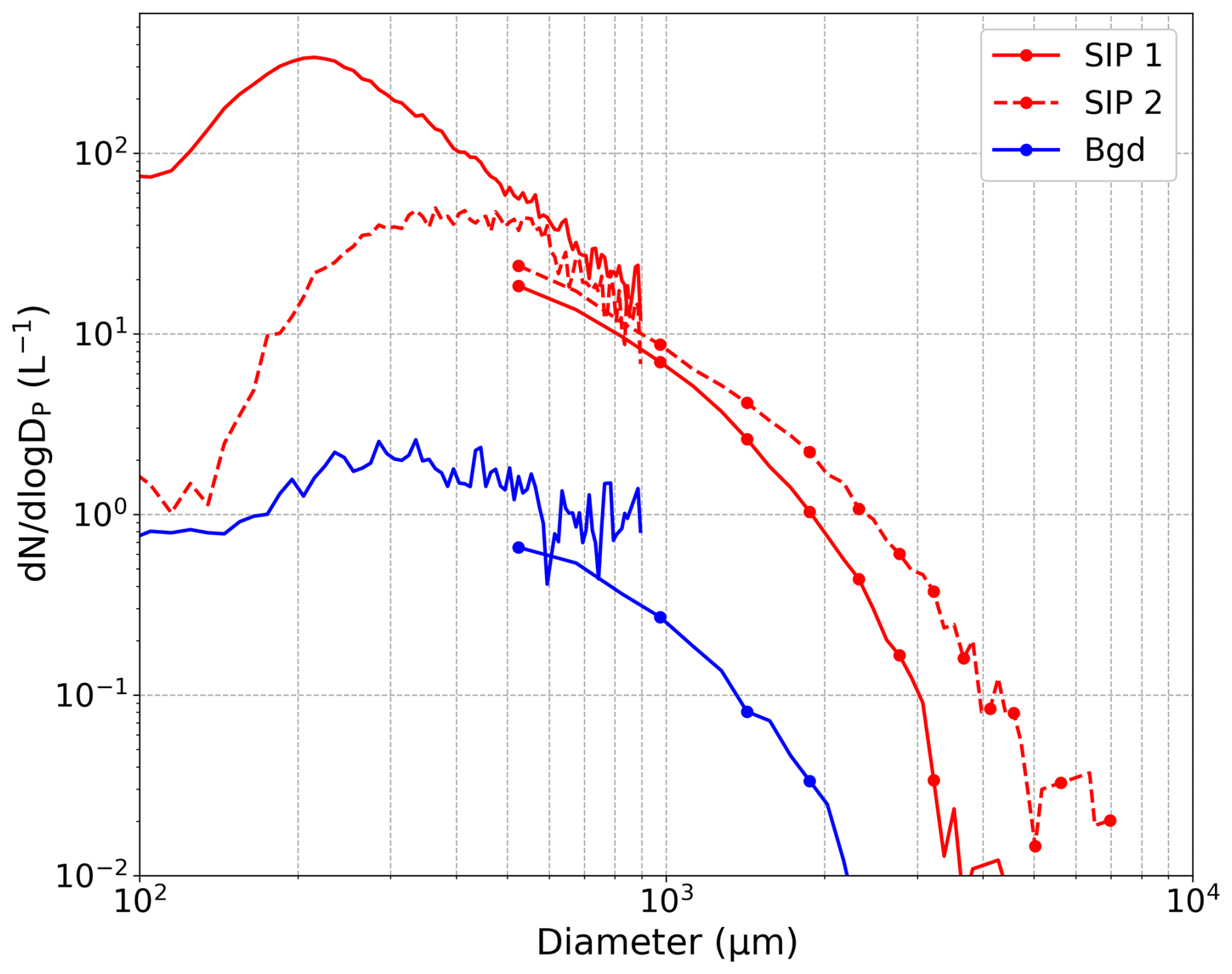
Figure 8 Mean composite (2D-S and HVPS) ice particle size distributions for SIP periods 1 (between 16:27:00 and 16:29:45 UTC) and 2 (between 16:19:45 and 16:20:30 UTC) (red lines) during flight C328 (31 October 2022), and two background ice periods (blue line). HVPS data shown by lines with markers for particle sizes > 600 µm.

SIP 2 occurred in a cumulus segment adjacent to SIP 1, with similar in-cloud temperatures; however, unlike in SIP 1, SIP 2 contained little evidence that the H–M process was active, with few observations of small columnar ice, or larger rimed crystals (Fig. C2), and very low supercooled liquid droplet concentrations (Fig. 6c). Given most of the observed ice crystals likely formed a considerable distance away from the measurement location, before growing over time to their observed final state, it is difficult to surmise the mechanisms responsible for their origins; although, there are several examples of distorted droplets, jetting and fragments of shattered drops in the CPI imagery (Fig. C2), indicative of some contribution from frozen droplet fragmentation. SIP 2 is likely an example of an old ice multiplication cell, within which SIP activity has accelerated liquid depletion via the WBF process and riming, quickly generating an almost fully glaciated (maximum μ₃ value of 0.91) and precipitating cloud region.

3.2.3 Case study 2 – Flight C329 on 1 November 2022

Figure 9 shows time series of selected cloud microphysical properties measured during flight C329; all sampled cloud segments were part of the convective CAO regime. Ice multiplication activity was detected more frequently here than during any other M-Phase flight, with 35 % of in-cloud measurements made within identified SIP periods. The mean ice particle concentration measured across SIP regions during C329 was 36.2 L⁻¹, varying from 1.5 L⁻¹ (5th percentile) up to 101.6 L⁻¹ (95th percentile).

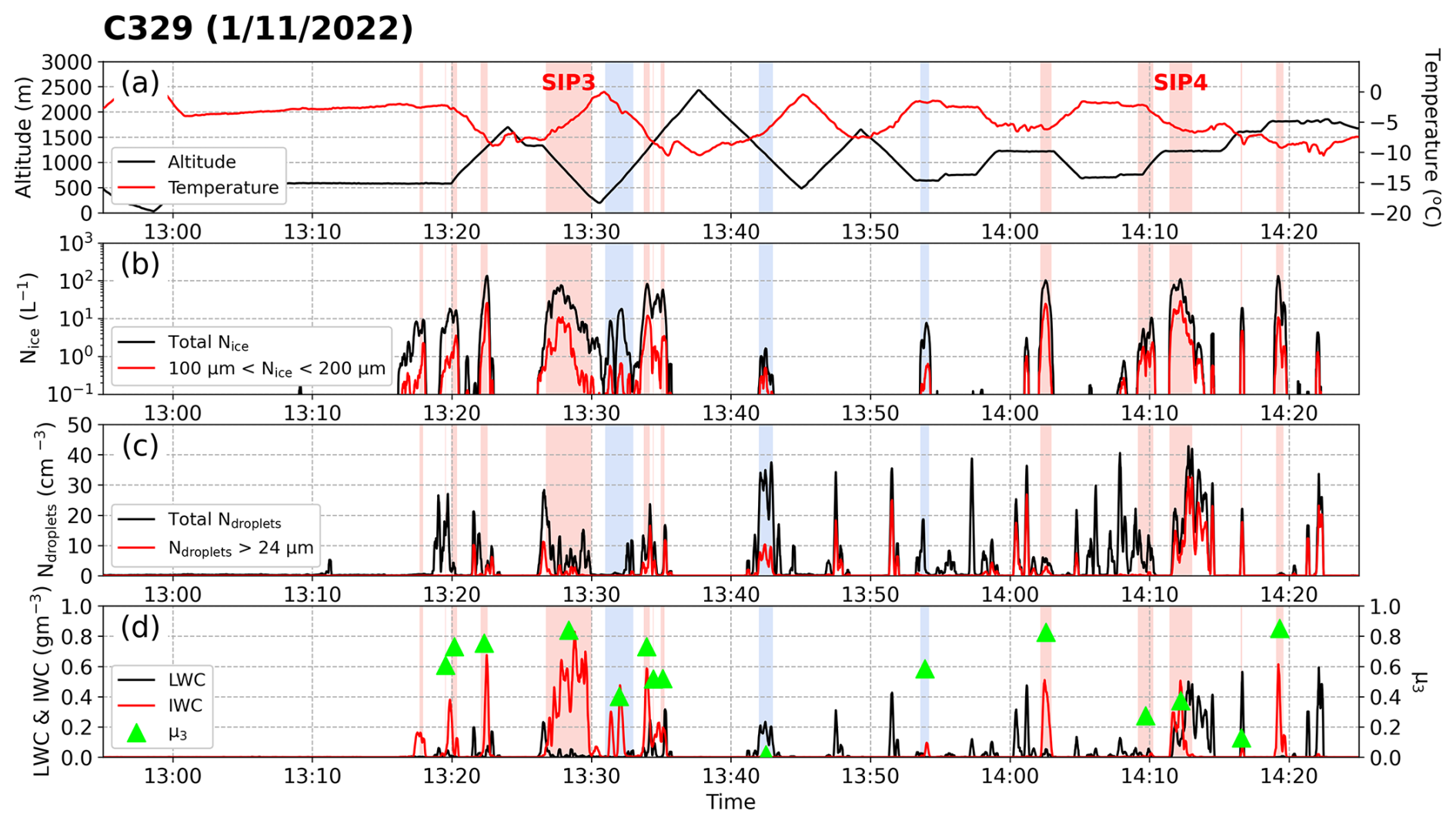
Figure 9 Time series of cloud microphysical properties (10 s averages) measured during flight C329 on 1 November 2022 (transit leg data excluded), including (a) local temperature (red line) and altitude (black line), (b) total ice crystal number concentration (N_ice; black line) and concentration of ice particles with diameter > 100 and < 200 µm (red line), (c) total cloud droplet concentration (N_droplets; black line) and concentration of cloud droplets with diameter > 24 µm (red line), and (d) liquid water content (LWC) and ice water content (IWC). SIP and background ice regions are shaded in red and blue, respectively. Mean ice mass fraction (μ₃) values for SIP and background ice periods are also marked in panel (d) (green triangles).

SIP periods 3 (SIP 3) and 4 (SIP 4) were sampled from 13:26:45 to 13:29:18 UTC and 14:11:25 to 14:13:03 UTC, respectively, and are marked in Fig. 9a. Measured in-cloud temperatures during both periods were well within the active range for the H–M process, ranging from −7.4 to −3.2 °C during the descending sawtooth leg in SIP 3, and across the SLR in SIP 4 the mean temperature was −6.2 °C.

Maximum measured 1 Hz ice concentrations were 95.2 L⁻¹ in SIP 3 and 145.5 L⁻¹ in SIP 4, with 12 % and 24 % of ice crystals observed during SIP 3 and SIP 4, respectively, having a diameter of less than 200 µm, indicating ice multiplication processes were likely active. This is reflected in the size distributions presented in Fig. 11, peaking between ice particle diameters of 250 and 350 µm for both SIP periods. The PSD for all background ice regions peaks at larger sizes of between 400 and 500 µm, indicative of more significant particle ageing relative to the neighbouring SIP regions.

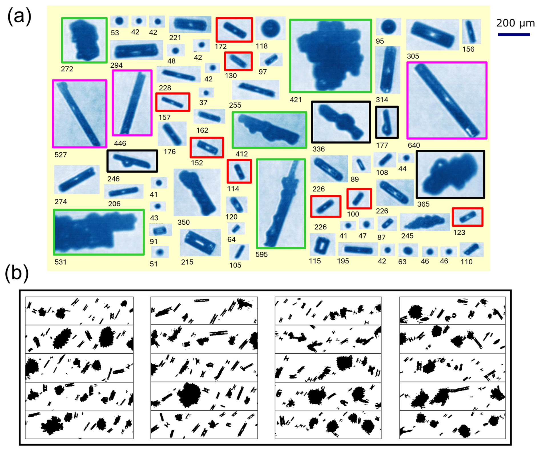
Figure 10 (a) Examples of cloud particles (ice crystals and liquid droplets) imaged with the CPI probe in SIP period 3 (between 13:26:45 and 13:29:18 UTC) during flight C329 (1 November 2022); subsets of small columnar ice of size < 200 µm (red frames), long columns (pink frames), rimed columns and plates (green frames), and columns with frozen droplets attached (black frames) are highlighted; numbers below images indicate the maximum dimension length (D_p) of each particle. (b) 2D-S images of highly irregular particles captured in SIP 3; the height of each strip corresponds to the 2D-S array width of 1280 µm.

The levels of glaciation of both cloud regions sampled during SIP 3 and SIP 4 were substantially different; the mean μ₃ during SIP 3 (0.83) was more than double that during SIP 4 (0.37), reflected by much higher supercooled liquid droplet concentrations in SIP 4 (${\stackrel{\mathrm{‾}}{N}}_{\mathrm{droplets}}$ = 23.9 cm⁻³) compared to SIP 3 (${\stackrel{\mathrm{‾}}{N}}_{\mathrm{droplets}}$ = 9.3 cm⁻³). In several previous in-situ observational studies, a strong liquid water presence has been considered a pre-requisite for the initiation of SIP processes (Lawson et al., 2017; Huang et al., 2022; Waitz et al., 2022); however, as discussed in Korolev et al. (2020), a lack of liquid droplets observed within a region of apparent SIP activity, such as SIP 3, may be explained by their evaporation due to the WBF process as well as significant riming prior to the cloud region arriving at the measurement point. Indeed, the CPI images presented in Fig. 10a indicate that riming was prevalent in SIP 3, with several examples of heavily rimed columns or plates (green frames); examples of droplets freezing on contact with large ice particles are also shown (black frames). The CPI imagery from SIP 3 also contains an abundance of small columns, some hollow (red frames), with D_p between 60 and 200 µm; this, in addition to the well-mixed regions of splinters, small columns and heavily rimed graupel particles shown in the 2D-S imagery (Fig. 10b) suggests the H–M process was active during SIP 3. Furthermore, the maximum ice particle size in SIP 3, measured with the HVPS probe, was ∼ 7 mm, compared to ∼ 3 mm in SIP 4 (Fig. 11), implying that the cloud segment sampled during SIP 3 was a more mature convective cell, within which the H–M process is known to operate particularly efficiently (Yang et al., 2020).

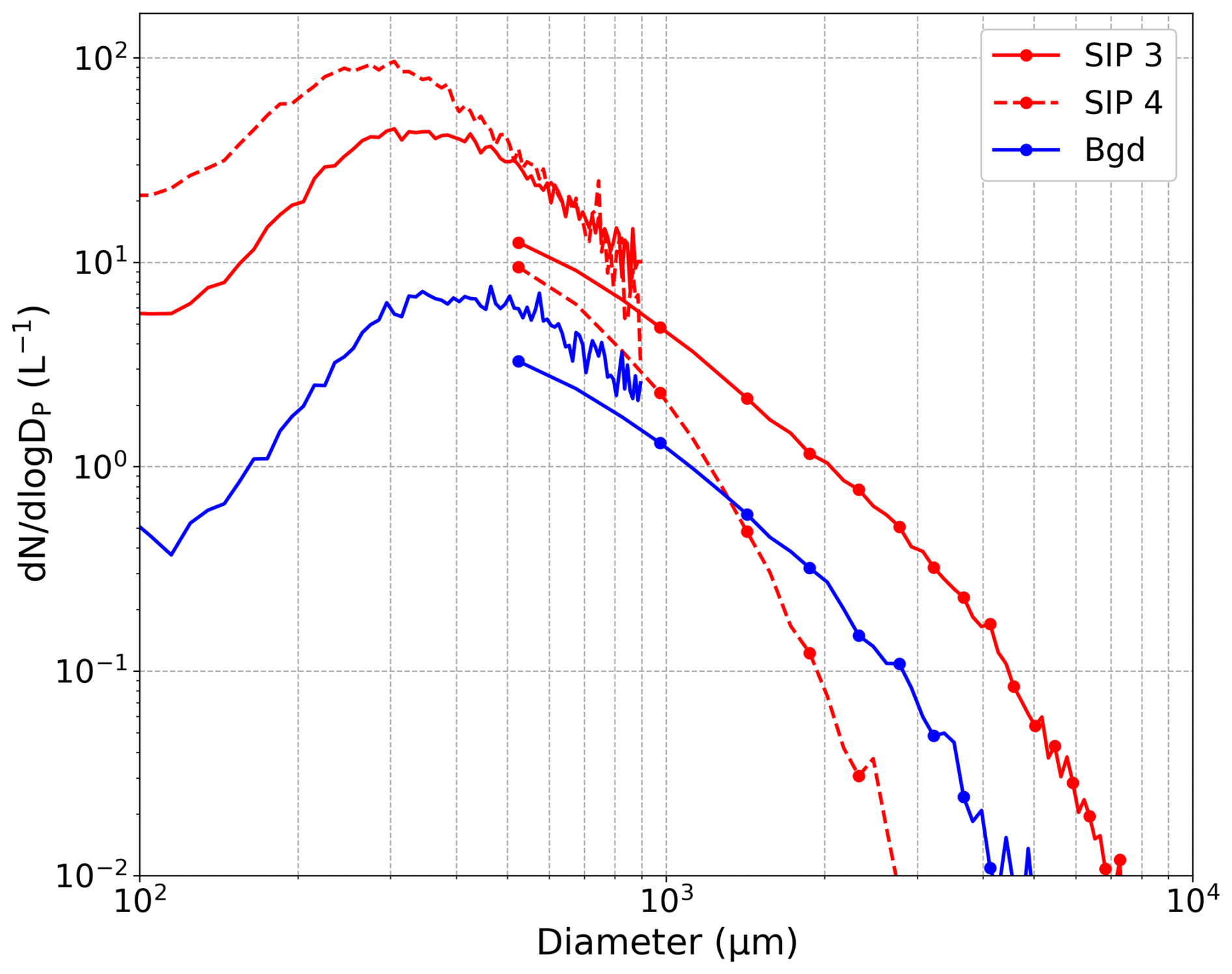
Figure 11 Mean composite (2D-S and HVPS) ice particle size distributions for SIP periods 3 (between 13:26:45 and 13:29:18 UTC) and 4 (between 14:11:25 and 14:13:03 UTC) (red lines) during flight C329 (1 November 2022), and all background ice periods (blue line). HVPS data shown by lines with markers for particle sizes > 600 µm.

The CPI and 2D-S images captured during SIP 4 (Fig. C3 in Appendix C) are similarly consistent with the H–M process being active and primarily responsible for the high ice concentration measurements; large, well-rimed columns, liquid droplets with D_p > 24 µm and small columns were all present within this cumulus cloud segment. Additionally, as SIP 4 was sampled during a constant altitude, SLR flight leg, we can look at how in-cloud turbulence may have affected ice multiplication; the mean vertical wind speed measured during SIP 4 was +0.94 ± 0.09 m s⁻¹, with a maximum value of +3.29 m s⁻¹, indicating updraft conditions dominated. It is well-documented that convective updrafts help provide favourable conditions for SIP processes by creating a more saturated environment for cloud droplet generation and growth (Hou et al., 2021; Qu et al., 2022; Wang et al., 2023).

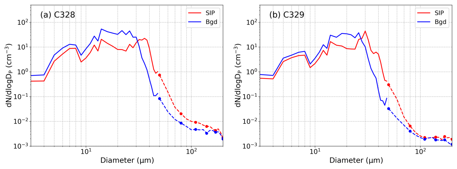
Figure 12 Mean cloud droplet size distributions measured with the CDP (D_P < 50 µm) for all SIP (red lines) and background ice periods (blue lines) during flights (a) C328, and (b) C329. 2D-S low irregular particle size distributions (dashed lines), used as proxy for large cloud droplets (D_P > 50 µm), are also provided.

The importance of large, supercooled liquid droplets in initiating SIP, and the H–M process in particular, is further emphasised by the cloud droplet size distributions shown in Fig. 12. Concentrations of droplets with diameter greater than ∼ 30 µm were substantially higher when averaged across SIP periods compared to neighbouring background ice regions during both flights C328 and C329 (Fig. 12). Interestingly, although there was clearly a strong presence of small liquid droplets (D_p < 12 µm) across SIP regions, consistent with the early experiments of Mossop (1978), their concentrations were generally higher across background ice regions. This suggests that certain mechanistic hypotheses for the H–M process may place too much importance on the role played by small droplets, such as that proposed by Choularton et al. (1980) regarding the symmetrical freezing and shattering of large droplets that impact regions of graupel particles where rime spires comprising small droplets have grown.

3.2.4 Splinter production rate

In this section, we explore the extent to which ice multiplication via the H–M process alone can account for the ice crystal enhancements measured during M-Phase. A splinter production rate (see Sect. 2.6) was estimated for each of the stratiform and convective cloud segments sampled throughout the campaign which had in-cloud temperatures falling within the H–M range, following Willis and Hallett (1991). As described in Sect. 2.6, our estimated rate of production of new ice crystals due to rime splintering, based on the assumption of gravitational collection of droplets by graupel particles, depends on in-situ measurements of graupel number concentration (ice crystals larger than 300 µm), graupel diameter and the concentration of liquid droplets with D_p > 24 µm; note, unlike the other commonly implemented splinter production rate formula derived by Harris-Hobbs and Cooper (1987), small liquid droplets (D_p < 12 µm) are not considered here. The Harris-Hobbs and Cooper (1987) calculation, used by Crosier et al. (2011) and Taylor et al. (2016), is based on the previously discussed theory of symmetrical droplet freezing and shattering, requiring the prior accretion of small droplets (Choularton et al., 1980; Griggs and Choularton, 1983). The formula adopted here (Eq. 4) assumes a much greater role played by large droplets, as described by Hallett et al. (1978); moreover, as shown in Fig. 12, concentrations of small liquid droplets were higher within background ice regions compared to SIP regions during M-Phase, thus calculating a splinter production rate that scales with increasing small droplet concentrations would not be consistent with the observations.

Table 4 Relationship between calculated splinter production rates $\left(\frac{\mathrm{d}{N}_{\mathrm{ice}}}{\mathrm{d}t}\right)$ and mean measured ice concentrations (N_ice) for all cloud segments sampled during M-Phase with in-cloud temperatures within the H–M range of −3 to −8 °C; separate relationships for stratiform and convective clouds are also derived. Timescales for N_ice increase from 1 to 100 L⁻¹ are calculated from each fitting function, including minimum and maximum timescales based on the relative uncertainty in the splinter production rate calculation (±86 %). Results from Mossop (1985c) and Järvinen et al. (2022) are also provided.

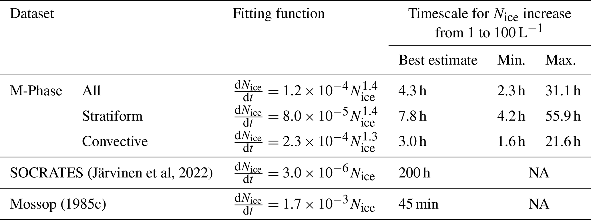
Rime splintering rates were calculated at 1 Hz resolution and averaged over the full cloud segment sampling duration. Figure 13 shows the calculated splinter production rate $\left(\frac{\mathrm{d}{N}_{\mathrm{ice}}}{\mathrm{d}t}\right)$ as a function of mean measured ice concentration (N_ice) for each individual cloud segment. For all relevant M-Phase clouds, the estimated splinter production rate can be expressed according to the power law relationship: $\frac{\mathrm{d}{N}_{\mathrm{ice}}}{\mathrm{d}t}=\mathrm{1.2}\times {\mathrm{10}}^{-\mathrm{4}}{N}_{\mathrm{ice}}^{\mathrm{1.4}}$ (Table 4). By integrating this relationship and assuming that all ice multiplication can be attributed to the H–M process, an increase in N_ice from 1 to 100 L⁻¹ (i.e. dN_ice) within a particular cloud region would take just over 4 h (i.e. dt) (Table 4). However, taking into consideration the overall relative uncertainty (±86 %) in the splinter production rate calculation (Sect. 2.6), an ice concentration increase of this magnitude due solely to the H–M process may occur over timescales as short as just over 2 h, or as long as ∼ 31 h (Table 4). This difference, of more than an order of magnitude, emphasises the need for improved rime splintering parameter constraints (Eq. 4) and real-time microphysical profiling to reduce uncertainty in future campaigns, enabling development of more robust and reliable SIP parameterisations for numerical modelling work.

Our range of estimated rime splintering timescales can be considered physically realistic for marine stratocumulus CAO clouds given their typical lifetime over the North Atlantic is known to vary from several hours to more than a day (Zhang et al., 2023). Broken cumulus cloud fields downstream of the regime transition are generally more short-lived, typically dissipating less than a few hours after forming (Murray-Watson et al., 2023); therefore, in the convective regime, only our fastest splinter production rate estimate for M-Phase can be deemed physically realistic. However, when sampled cumulus cloud segments are considered in isolation, we estimate that the H–M process can drive ice crystal enhancements on the order of 100 L⁻¹ in a more reasonable time of around 3 h (and as fast as ∼ 1.5 h) (Table 4).

Note, as discussed in Sect. 2.1.1, particles of D_p < 100 µm were excluded from our analysis given the likelihood that they would be heavily contaminated with out-of-focus liquid droplets. However, if in-situ measurements are made within a few minutes of the onset of SIP, we would expect to measure high concentrations of particles smaller than 100 µm, following previously reported ice crystal depositional growth rates within the H–M process temperature range (Fuchs et al., 2025). Therefore, as an upper-bound estimate, if we assume that all HI particles detected with the 2D-S of size less than 100 µm were ice crystals, N_ice will increase on average by ∼ 45 % in stratiform and ∼ 10 % in convective cloud regions (Fig. D1a in Appendix D); subsequent glaciation timescales by rime splintering are estimated to increase to ∼ 7 h (all clouds), ∼ 4 h (convective), and ∼ 19 h (stratiform), i.e. around a factor of two. However, the bimodal PSDs (and 2D-S imagery) shown in Fig A1 strongly indicate that a large fraction of particles < 100 µm were likely not ice crystals, but instead out-of-focus droplets (Sect. 2.1.1), thus our $\frac{\mathrm{d}{N}_{\mathrm{ice}}}{\mathrm{d}t}$–N_ice relationships and glaciation timescales presented in Table 4 can still be considered reasonable approximations of conditions during M-Phase. Ultimately, these glaciation timescale estimates act as order-of-magnitude feasibility tests for the H–M process dominating in marine CAO clouds; however, given the large uncertainty (±86 %) in calculated splinter production rates, strong contributions from other SIP mechanisms cannot be entirely ruled out.

During M-Phase, sampled cumulus clouds were often weakly convective, with measured updraft speeds most commonly falling between 0 and 1 m s⁻¹ (Fig. 4f); at 0.5 m s⁻¹, it would take approximately one hour for air to mix over the full vertical extent of a 2 km deep cloud region. As this convective overturning timescale is considerably faster than our best estimates for glaciation timescales due to the H–M process alone (Table 4), we would expect to observe peak ice particle concentrations across the full sampled cloud depth, rather than at specific temperatures which may be more conducive to the H–M process. Indeed, this is consistent with measurements during both case studies presented in Fig. 5; N_ice values exceeding ∼ 100 and ∼ 50 L⁻¹ were observed across most in-cloud temperatures (∼ −5 to −10 °C) during flights C328 and C329, respectively.

Another way to quantitatively evaluate our estimated splinter production rates for M-Phase is by comparing them to the actual rate of ice formation required to maintain high concentrations of small ice particles, characteristic of SIP periods (Figs. 8 and 11), based on previously reported depositional growth rates of ice crystals at temperatures within the H–M range (Ryan et al., 1976; Fuchs et al., 2025). To this end, if we consider an ice concentration of 10 L⁻¹ and assume this is composed entirely of particles between 100 and 200 µm, then further assume a steady-state size distribution within this particle size range and an approximate ice crystal growth rate of 0.5 µm s⁻¹ (derived at ∼ −5 °C by Fuchs et al., 2025), an ice particle formation rate of around 0.05 L⁻¹ s⁻¹ would be required to maintain equilibrium between ice crystals growing into and out of the 100 to 200 µm size range. This ice formation rate is about an order of magnitude higher than the corresponding splinter production rate determined here for an ice concentration of 10 L⁻¹ (Fig. 13), suggesting that the H–M process can only quantitatively account for ∼ 10 % of observed ice crystals. However, the splinter production rates shown in Fig. 13 should be viewed as conservative estimates given they represent averages across full cloud segments; rime splintering rates depend on graupel and large liquid droplet concentrations (Eqs. 3 and 4), both inhomogeneous properties within clouds, producing strong in-cloud spatial variability in splinter production rates. Therefore, we also present the maximum splinter production rate as a function of maximum N_ice for each cloud segment in Fig. D1b in Appendix D; this suggests that the H–M process may account for ∼ 50 % of ice crystal formation within regions where ice concentrations are highest and thus where SIP is likely to be most active. As discussed previously, it is likely that other SIP mechanisms (e.g. frozen droplet fragmentation) were acting concurrently within the H–M zone, which would further account for the discrepancy between our estimated rime splintering and ice formation rates.

Figure 13 also shows splinter production rates estimated by Mossop (1985c) and Järvinen et al. (2022), following the same approach as used in this study, for wintertime cumulus clouds over Australia, and summertime CAO clouds over the Southern Ocean during the SOCRATES campaign, respectively. Mossop (1985c) determined that rime splintering could generate ice crystal enhancements on the order of 100 L⁻¹ in ∼ 45 min, implying that the H–M process was active and dominating over other SIP mechanisms. In contrast, Järvinen et al. (2022) concluded that the splinter production rate estimated for marine CAO clouds over the Southern Ocean was too slow to explain the observed level of ice multiplication; estimated cloud glaciation timescales of approximately 200 h far exceeded the typical lifetime of Southern Ocean stratocumulus clouds. Other mechanisms such as ice-ice collisions and frozen droplet shattering were therefore considered to be contributing significantly to SIP.

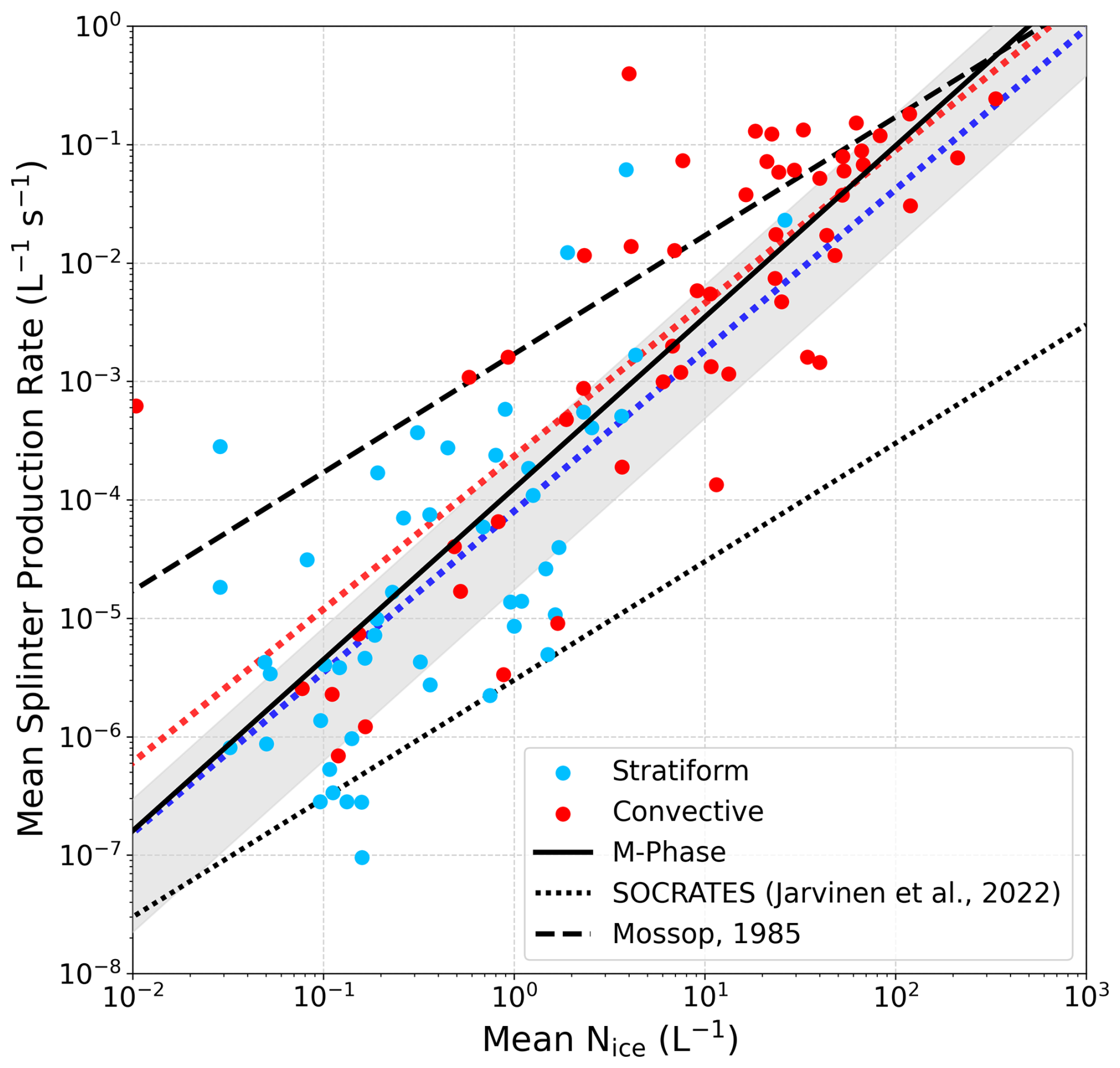
Figure 13 Mean splinter production rate $\left(\frac{\mathrm{d}{N}_{\mathrm{ice}}}{\mathrm{d}t}\right)$, calculated following Willis and Hallett (1991), as a function of mean measured ice particle concentrations for individual stratiform (blue) and convective (red) cloud segments with in-cloud temperatures within the H–M range of −3 to −8 °C. The solid black line represents the fit through the M-Phase data; the shaded region covers the area between fitting functions determined from maximum and minimum splinter production rates based on the overall relative uncertainty of ±86 %. The dashed and dotted black lines represent the relationships estimated by Mossop (1985c) (wintertime cumulus clouds over Australia) and Järvinen et al. (2022) (summertime CAO clouds over Southern Ocean), respectively.

It is reassuring to note that the range of splinter production rates calculated by Harris-Hobbs and Cooper (1987) for mixed-phase cumulus clouds at several locations across the United States (∼ 10⁻⁴ to 10⁰ L⁻¹ s⁻¹), using their alternative formula that incorporates small liquid droplets (D_p < 12 µm), is comparable to our results for M-Phase (Fig. 13); both studies sampled cumulus clouds of similar microphysical characteristics. Mean concentrations of large, supercooled liquid droplets (D_p > 24 µm) during two of the three aircraft campaigns discussed in Harris-Hobbs and Cooper (1987) (3.7 and 5.6 cm⁻³ in California and Montana, respectively) were strikingly similar to those observed within cumulus clouds during M-Phase (4.8 cm⁻³). Large droplet concentrations were much higher during the other campaign (16 L⁻¹ in Florida); however, this difference is compensated for to some extent by the graupel concentrations that were on average an order of magnitude greater during M-Phase. Finally, although updraft speeds were a factor of 2–3 greater in the Harris-Hobbs and Cooper (1987) study than measured during M-Phase, the role of turbulence in initiating and sustaining rime splintering remains uncertain, with some evidence suggesting that weak-to-moderate rather than strong updrafts are more favourable for ice multiplication (Hallett et al., 1978; Sullivan et al., 2017).

Overall, we estimate significant differences between glaciation timescales in the stratiform and convective regimes during M-Phase (Table 4), implying that numerical models incorporating a single parameterisation scheme for the H–M process across all cloud types may misrepresent the spatial and temporal distribution of mixed-phase cloud glaciation, with liquid-phase conditions likely overestimated in the convective regime. To address this, we recommend the application of regime-aware SIP parameterisations into larger scale cloud microphysics schemes, where SIP activation depends not only on temperature thresholds and droplet size distributions but also on dynamical context, such as updraft strength and cloud morphology. Improving the representation of SIP variability across CAO regimes in climate and NWP models is critical for properly capturing the transition from liquid- to ice-dominated, optically thinner states, thereby reducing biases in simulated cloud radiative fluxes and the onset of light precipitation in high-latitude maritime environments.

3.2.5 Evidence of ice-ice collisional breakup

In Sect. 3.1, we showed that a secondary peak in SIP activity was observed at colder in-cloud temperatures during M-Phase, consistent with results from laboratory studies indicating that the collisional breakup of large, fragile ice particles is most efficient at around −16 °C (Vardiman, 1978; Takahashi et al., 1995; Grzegorczyk et al., 2023); fragile dendritic branches, particularly susceptible to fragmentation upon collision, are known to grow preferentially by vapour deposition at this temperature (Ryan et al., 1976; Takahashi et al., 1995).

Flight C326 took place on 28 October 2022 and utilised sawtooth profiles throughout, initially sampling stratiform cloud during the outbound leg over the Labrador Sea, which broke up into convective elements for the return leg. Cloud top temperatures as low as ∼ −19 °C were reached, corresponding to a maximum theoretical N_ice from primary ice production (i.e. N_INP) of ∼ 1 L⁻¹ (Fig. 14); very similar N_ice and N_INP were observed at ∼ −19 °C (Fig. 14) suggesting primary ice production via immersion freezing, rather than SIP, was dominant at cloud top. The highest ice particle concentrations during flight C326 were measured between −15 and −18 °C, reaching 37.4 L⁻¹, which exceeded the associated N_INP by around 1–2 orders of magnitude (Fig. 14); Takahashi et al. (1995) observed a clear peak in the number of ice crystals ejected following collisions at ∼ −16 °C, sharply decaying at colder temperatures towards −20 °C, which is consistent with the comparable N_ice and N_INP observed at cloud top during flight C326. Järvinen et al. (2022) reported similar ice crystal enhancements within this temperature range in Southern Ocean stratocumulus clouds. This ice enhancement is considerably smaller than that observed within the H–M temperature zone during M-Phase (Sect. 3.2.1); however, previous airborne studies in shallow stratiform clouds have observed N_ice exceeding several hundred per litre where cloud tops extend past temperatures lower than ∼ −15 °C (Rangno and Hobbs, 2001; Yang et al., 2014). Therefore, ice multiplication within this colder temperature region may have the potential to substantially modify cloud albedo; thus, improving our understanding of the active SIP mechanism is important for future modelling studies to fully capture the radiative effects of CAO clouds.

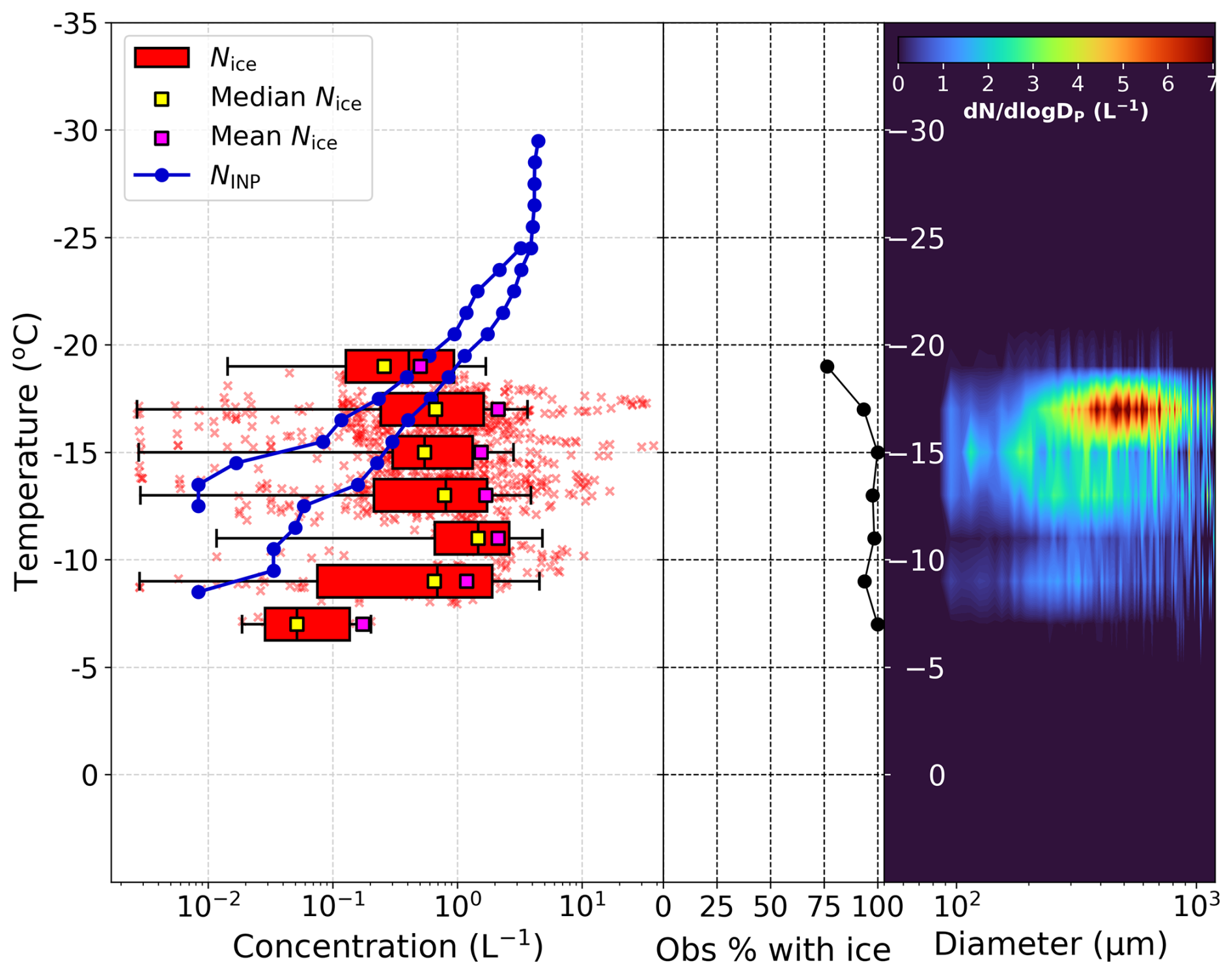
Figure 14 Measured total (2D-S + HVPS) ice crystal number concentrations (N_ice; red) as a function of local in-cloud temperature (1 Hz data) for flight C326 (28 October 2022). Boxplots (red) for N_iceabove the instrument detection limit in 2 °C temperature bins are composed of centre lines, edges and whiskers representing the median, interquartile range (25th to 75th percentile) and nearest data points within 1.5 × interquartile range of the lower and upper quartiles, respectively. Median N_ice (yellow squares) and mean N_ice (pink squares) are calculated from all data points, including N_ice below the instrument detection limit (i.e. where we have set N_ice to 0 L⁻¹). The percentage of ice concentration observations above 0 L⁻¹ within each temperature bin is also provided (black line). Measured INP concentrations (N_INP) derived from filter samples collected during flight C326 are shown in blue. Mean ice particle size distributions as a function of local in-cloud temperature are presented in the right panel.

During C326, sampled cloud regions with temperatures between −15 and −18 °C were heavily populated with large ice crystals of D_p between 400 and 800 µm (Fig. 14). The ice breakup mechanism has been found to readily initiate in similar cloud regions where ice particles with a broad range of sizes are well-mixed, as fragmentation upon impact between ice crystals is most efficient when the difference in their terminal fall velocities is large, maximising the kinetic energy of the collision (Hoarau et al., 2018; Korolev and Leisner, 2020).

3.2.6 Case study 3 – Flight C326 on 28 October 2022

Figure 15 shows time series of selected cloud microphysical properties measured during flight C326. SIP periods 5 (SIP 5) and 6 (SIP 6) were observed from 17:55:40 to 17:56:08 UTC and 19:34:40 and 19:35:10 UTC, respectively, and are marked in Fig. 15. Mean measured temperatures during SIP 5 and SIP 6 were −13.9 and −17.0 °C, respectively; both SIP periods were observed in cloud segments which spanned the temperature range consistent with efficient ice-ice collisional breakup, according to the previously mentioned laboratory experiments (Vardiman, 1978; Takahashi et al., 1995; Grzegorczyk et al., 2023), with cloud top temperatures in both cases reaching ∼ −18 °C.

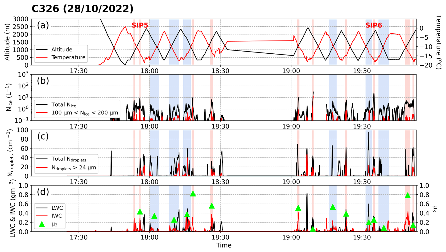
Figure 15 Time series of cloud microphysical properties (10 s averages) measured during flight C326 on 28 October 2022 (transit leg data excluded), including (a) temperature (red line) and altitude (black line), (b) total ice crystal number concentration (N_ice;black line) and concentration of ice particles with diameter > 100 and < 200 µm (red line), (c) total cloud droplet concentration (N_droplets; black line) and concentration of cloud droplets with diameter > 24 µm (red line), and (d) liquid water content (LWC) and ice water content (IWC). SIP and background ice regions are shaded in red and blue, respectively. Mean ice mass fraction (μ₃) values for SIP and background ice periods are also marked in panel (d) (green triangles).

The maximum ice particle concentration (1 Hz data) measured in SIP 5 was 16.6 L⁻¹ and the corresponding PSD (Fig. 16) peaked between particle sizes of 350 and 550 µm, with a maximum D_p of ∼ 5 mm. This broad size distribution suggests that ice crystals of varying stages of growth were collocated during SIP 5, thus meeting the requirement for ice breakup that colliding particles have greatly varying vertical velocities (Korolev and Leisner, 2020).

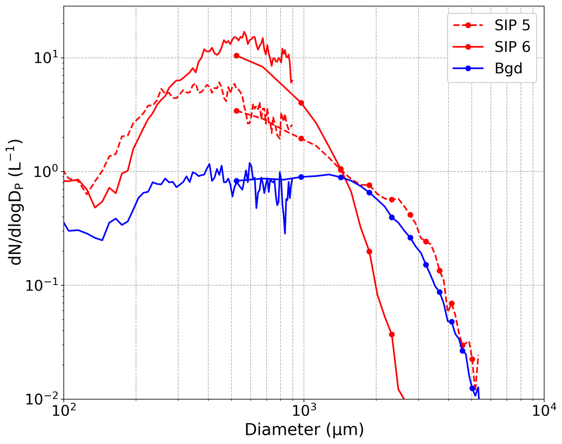
Figure 16 Mean composite (2D-S and HVPS) ice particle size distributions for SIP periods 5 (between 17:55:40 and 17:56:08 UTC) and 6 (between 19:34:40 and 19:35:10 UTC) (red lines) during flight C326 (28 October 2022), and all background ice periods (blue line). HVPS data shown by lines with markers for particle sizes > 600 µm.

During SIP 6, measured ice particle concentrations reached 32.2 L⁻¹ and the corresponding size distribution peaked at larger crystal diameters than during SIP 5 (500 µm < D_p < 800 µm), consistent with original assumptions by Vardiman (1978) that small ice particles do not have elaborate enough geometry or sufficiently large terminal velocity to fragment upon collision. During SIP 6, the observed PSD was narrower overall than in SIP 5, with a maximum ice crystal size of ∼ 3 mm. The relative lack of growth experienced by particles observed during SIP 6, compared to SIP 5, suggests that ice multiplication by ice-ice collisions occurred more recently in SIP 6. Furthermore, SIP 6 was sampled closer to cloud top than SIP 5; ice crystals observed during SIP 5 may have also formed near cloud top before growing while mixing or precipitating down to the point of observation, as evidenced by the images of large, branched crystals shown in Fig. 17.

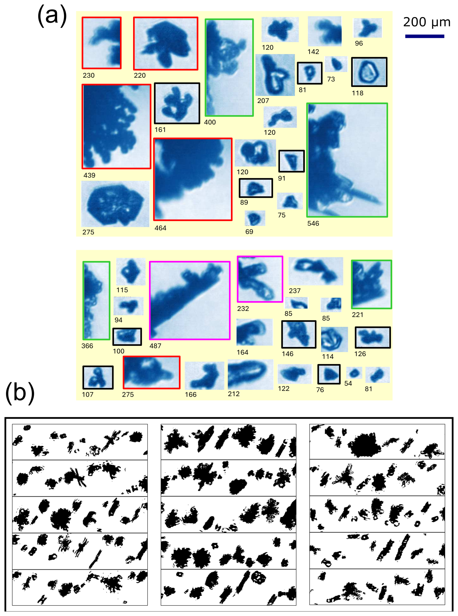
Figure 17 (a) Examples of cloud particles (ice crystals and liquid droplets) imaged with the CPI probe in two cloud segments (cloud top temperature ∼ −18 °C) during flight C326 (28 October 2022); subsets of large rimed crystals with fragile branches (red frames), aggregates (green frames), large crystals with plate-like extensions (pink frames), and small, irregular ice fragments (black frames) are highlighted; numbers below images indicate the maximum dimension length (D_p) of each particle. (b) 2D-S images of highly irregular particles captured in both cloud segments; the height of each strip corresponds to the 2D-S array width of 1280 µm.

Mean μ₃ values for both SIP 5 (0.43) and SIP 6 (0.34) were considerably lower than those discussed previously for SIP 1 to SIP 4. These less glaciated cloud regions, reflecting a strong supercooled liquid water presence, are consistent with previous studies in which ice-ice collisional breakup was found to favour heavy riming conditions at temperatures well-below the active H–M zone (Karalis et al., 2022); fragile dendritic branches have been observed to grow particularly efficiently on heavily rimed particles (Pruppacher and Klett, 1997). Figure 17 presents CPI and 2D-S images of ice particles sampled in two cloud segments during flight C326, both with cloud top temperatures of ∼ −18 °C. Large, heavily rimed ice crystals with fragile protuberances or branches were frequently observed (red frames), alongside aggregates (green frames) and large irregular crystals with plate-like extensions (pink frames) (Fig. 17a); collisions between such particles with differing, often brittle, surface properties are most likely to cause ice breakup, producing high concentrations of small, irregular ice fragments (black frames).

Ultimately, the in-situ evidence presented here supporting active ice-ice collisional breakup during M-Phase can contribute towards constraining new physics-based model parameterisations, such as the scheme developed by Phillips et al. (2017) described in Sect. 1, that require information on the temperatures, ice mass fractions and ice particle sizes and morphologies most conducive to initiating the ice breakup process in shallow, marine CAO clouds.

3.3 Summary of environmental conditions favourable for SIP

Analysis of cloud microphysical properties measured during several ice multiplication episodes, as well as high-resolution ice crystal imagery and splinter production rate calculations (Sect. 3.2), indicates that the H–M process was likely the primary contributor to SIP within the CAO clouds sampled during M-Phase; however, concurrent SIP mechanisms are required to reconcile estimated ice formation rates, consistent with evidence of frozen droplet fragmentation also operating sporadically within the H–M temperature zone, shown in Figs. 7 and C1. Ice-ice collisional breakup was determined to be the most efficient SIP process in deeper cloud regions with cloud tops extending to temperatures below ∼ −15 °C. Figure 18 shows a series of normalised frequency distributions of in-situ data measured throughout the full campaign, highlighting the environmental conditions that correlate most strongly with SIP activation; measurements during SIP periods, as defined in Sect. 3.2, are compared with in-cloud observations made outside of SIP periods (i.e. Non-SIP in Fig. 18).

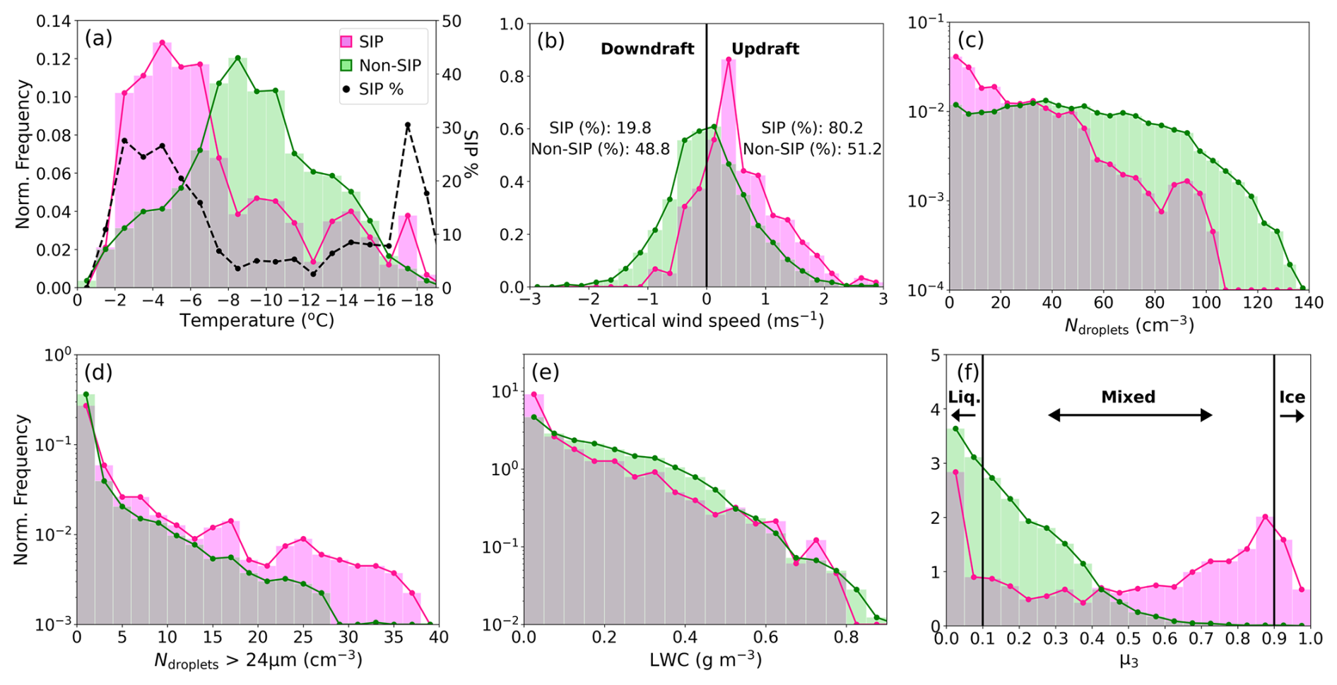
Figure 18 Relative frequency histograms of cloud microphysical properties (1 Hz data) measured within cloud regions containing strong evidence of active ice multiplication (SIP; pink), and those containing minimal evidence of active SIP processes (Non-SIP; green), including (a) local in-cloud temperature (percentage of total observations made during SIP periods within each 1 °C temperature bin also marked with dashed black line), (b) vertical wind speed (straight-and-level runs only), (c) total cloud droplet concentration (N_droplets), (d) concentration of cloud droplets with diameter > 24 µm, (e) liquid water content (LWC), and (f) ice mass fraction (μ₃) with thresholds for liquid, mixed and ice phase cloud regions marked. Data normalised so that area under both SIP and Non-SIP histograms integrates to 1.

Across all identified SIP periods, ice multiplication processes were observed to be most active between −3 and −6 °C (Fig. 18a); strong evidence of SIP was observed in 25 % of in-cloud measurements within this temperature range. A secondary peak in SIP activity was observed at colder temperatures between −16 and −18 °C, consistent with findings from early laboratory studies of ice-ice collisional break-up (Vardiman, 1978; Takahashi et al., 1995; Grzegorczyk et al., 2023). The weaker SIP mode detected between −9 and −12 °C (Fig. 18a) is likely related to aged secondary particles generated within the H–M zone that have been lifted in convective updrafts towards cloud top.

SIP periods were predominantly observed in updrafts (80 %), particularly low turbulence, weak updraft (< +0.5 m s⁻¹) regions, but also frequently in moderate updrafts of up to ∼ +2 m s⁻¹ (Fig. 18b); this relationship is even stronger (90 %) when vertical wind speeds measured within the H–M temperature zone are isolated (Fig. D2 in Appendix D). As previously discussed, updrafts provide a favourable environment for SIP, and particularly rime splintering, by supplying moisture to generate sufficient water supersaturation for the activation of aerosol into cloud droplets, which grow efficiently within updrafts to the necessary size (D_p > 24 µm) for riming and the initiation of the H–M process. Hallett et al. (1978) also observed peak splinter production within weak updrafts in cumulus clouds at temperatures between −4 and −6 °C; ice particles could be retained within this temperature zone long enough for the positive feedback process of splinter production, growth, riming and renewed splintering to occur. Heymsfield and Willis (2014) similarly suggested that locations where weak updrafts balance rimer fall speeds are most favourable for the H–M process as the time scales for riming are prolonged, enabling a more continuous production of secondary ice splinters. It should also be noted that more turbulent conditions, with updrafts regularly exceeding 3 m s⁻¹, have been found previously to be particularly conducive to strong SIP, as reported by Wang et al. (2023) in shallow mixed-phase clouds over China. However, in that case, as ice multiplication was determined to have mostly occurred at temperatures below the H–M zone, where graupel concentrations were very low, SIP was not attributed to the H–M process; instead, frozen droplet fragmentation was considered to be dominating, given the stronger updrafts facilitated the growth of many precipitation-sized liquid droplets that were collocated with high concentrations of small ice fragments.

The highest total cloud droplet concentrations were measured within non-SIP cloud segments reaching up to 140 cm⁻³ (Fig. 18c). However, concentrations of supercooled liquid droplets with D_p > 24 µm, considered necessary for the H–M process, were generally higher in SIP than in non-SIP regions (Fig. 18d). The importance of supercooled liquid water in initiating ice multiplication, and specifically the H–M process, is further emphasised by Fig. D2, which shows that peak LWC values (0.4–0.8 g m⁻³) were more frequently observed in SIP than in non-SIP regions. Fully glaciated SIP regions (μ₃ > 0.9) were occasionally detected during M-Phase (Fig. 18f); as discussed in Sect. 3.2.3, liquid water depletion and subsequent ice particle multiplication and growth may have occurred shortly before sampling in some cases.

In summary, SIP activity observed during M-Phase favoured: (a) the H–M temperature range, specifically from −3 to −6 °C, (b) updraft conditions, particularly low turbulence, quiescent regions, and (c) high concentrations of liquid droplets with diameter greater than 24 µm, consistent with the early rime splintering laboratory studies of Hallett and Mossop (1974) and Mossop (1978).

Overall, we observed strong evidence of ice multiplication in ∼ 15 % of in-cloud ice measurements (1 Hz data) throughout the campaign, which increases to ∼ 26 % within the H–M temperature zone. Specifically, SIP was significantly more active in the convective CAO regime; ∼ 46 % of ice measurements in convective cloud regions were made within SIP periods, compared to only ∼ 4 % in stratiform cloud. Note that this regime-specific quantification of SIP frequency is limited by (a) our general methodology that was based on manually identifying distinct regions of strong SIP activity, possibly leading to some weaker regions of ice multiplication being excluded, with SIP frequency in less turbulent stratiform cloud, in particular, likely underestimated, and (b) the previously discussed sampling biases in convective cloud regions towards warmer in-cloud temperatures, which are more conducive to SIP activity.

4 Conclusions

For this work, we investigated ice multiplication processes active in shallow, mixed-phase clouds embedded within CAOs through detailed analysis of in-situ airborne observations from the M-Phase campaign, which took place in October and November 2022 over the Labrador Sea in the North Atlantic Ocean. Measurements of cloud microphysical and thermodynamic properties were sub-divided into stratiform and convective CAO regimes to explore how SIP activity may evolve as uniform, stratocumulus cloud decks deepen and break up into cumulus clouds downwind over the warming sea surface. We identified explicit periods of SIP activity, based on ice crystal enhancement regions and high-resolution ice particle imagery, allowing the key markers and most favourable environmental conditions for specific SIP mechanisms to be defined. Figure 19 schematically summarises this study's key findings.

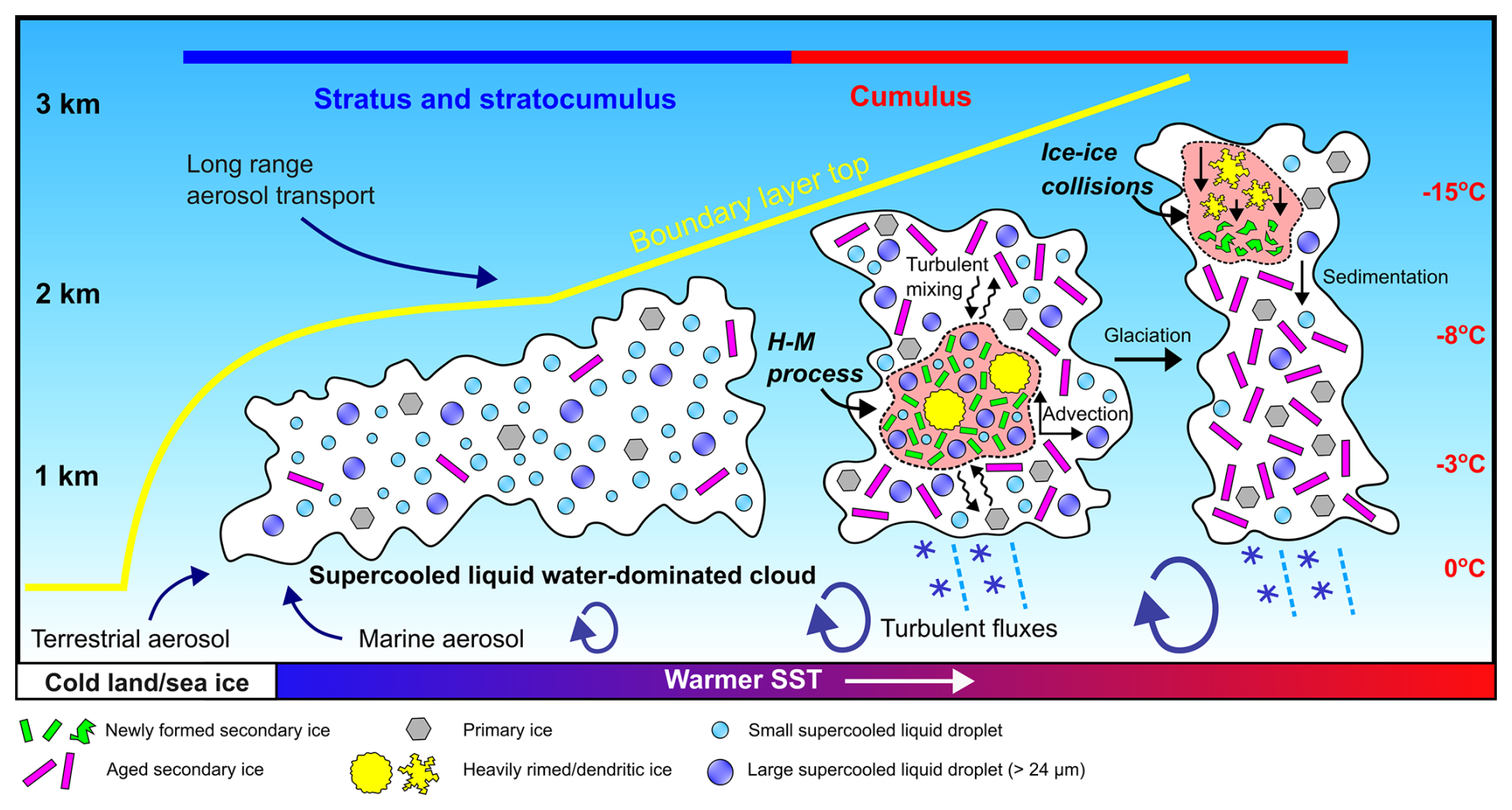
Figure 19 A schematic diagram summarising the evolution of cloud morphology and microphysical properties within CAOs, moving downwind from the stratiform to the convective regime, over the Labrador Sea during the M-Phase campaign. Red regions within cumulus cloud segments contain representations of the dominant SIP mechanisms, inferred from in-situ airborne observations.

Ice multiplication processes appeared to be active across the full range of temperatures (0 to −19 °C) observed within the CAO clouds sampled during M-Phase; however, SIP activity clearly peaked within the active temperature range for the H–M process, with the highest ice concentrations measured at ∼ −8 °C, exceeding 450 L⁻¹, more than four orders of magnitude above the expected N_INP. Identified SIP regions were usually well-populated with large, heavily rimed columnar ice crystals or graupel particles mixed with high concentrations of small columns (diameter less than 200 µm) or splinters, and large liquid drops (D_p > 24 µm), indicative of active rime splintering.

We estimated a splinter production rate for all cloud segments with temperatures within the H–M range, following the conceptual model by Hallett et al. (1978), and determined that the H–M process could feasibly fully account for sporadic but potentially strong SIP in the stratiform regime but may not be fast enough to realistically drive ice crystal enhancements regularly exceeding 100 L⁻¹ in shallow, cumulus clouds. However, when convective cloud regions were considered in isolation, we calculated a shorter glaciation timescale (∼ 3 h), more closely aligning with the expected lifetime of maritime cumulus clouds. Consequently, we suggest that regime-dependent parameterisations for the H–M process are needed for climate and NWP models to best capture the transition from liquid-dominated to well-glaciated CAO cloud states.

Some evidence of frozen droplet fragmentation operating concurrently with the H–M process was found at temperatures warmer than ∼ −10 °C. Frozen drops, some with protruding spicules indicative of jetting, were observed within SIP regions otherwise containing the key markers of active rime splintering; therefore, it's likely that multiple SIP mechanisms can activate simultaneously to generate the largest ice enhancements. However, beyond the limited qualitative image evidence indicating that frozen droplet fragmentation is occasionally active within the H–M zone, we are unable to quantify how much the mechanism contributes to secondary ice particle concentrations in this study.

A secondary peak in SIP activity was detected between −15 and −18 °C, consistent with the temperature range in which laboratory studies investigating ice-ice collisional breakup have observed maximum fragment ejection from collisions between graupel and fragile, dendritic ice crystals. Particle size distributions had a broad peak at larger ice crystal sizes (∼ 350 to 800 µm) than during rime splintering-dominated periods (∼ 200 to 500 µm). CPI images of heavily rimed, branched crystals and large aggregates were consistent with previous laboratory findings indicating that the ice breakup mechanism is most efficient when involving collisions between particles with substantially different terminal velocities and surface properties to maximise the kinetic energy upon impact.

Overall, we found that SIP mechanisms, particularly the H–M process, were more likely to initiate in weak-to-moderate updraft (< 2 m s⁻¹) regions which contain high concentrations of large liquid drops (D_p > 24 µm); conditions that were substantially more prevalent in the broken, cumulus clouds sampled during M-Phase than in the stratocumulus cloud decks. We recommend that future modelling of SIP in CAO clouds incorporate these findings through schemes depending not only on pre-defined temperature ranges and cloud droplet size distributions, but also on cloud dynamics (i.e. updraft strength) and morphologies.

In this study, we infer ice multiplication activity from in-situ ice particle concentration measurements and ice crystal imagery. This approach is limited by the lack of information available on where in the cloud the ice particles were generated; primary or secondary ice detected by the on-board instrumentation may have formed in the vicinity of the aircraft or may have sedimented down from nearer cloud top or mixed in from elsewhere. During M-Phase, we observed many fully glaciated SIP regions within the H–M temperature range, suggesting that liquid consumption by riming or the WBF process and subsequent ice crystal growth and multiplication had occurred before the point of observation. Future work would greatly benefit from the application of new, automatic ice crystal habit classification techniques to help efficiently determine the dimensions and growth time of each particle, as in Korolev et al. (2020) and Jaffeux et al. (2022); thus, the ice crystals that have likely formed in the environmental conditions corresponding with the measurement location can be separated from those originating elsewhere.

This study provides important information for future numerical modelling studies on the key SIP processes active within the shallow, marine boundary layer CAO clouds that frequently develop over the North Atlantic Ocean. Improved representation of spatiotemporal variations in mixed-phase cloud glaciation across the stratiform and convective CAO regimes may help reduce biases in simulated radiative fluxes, thereby reducing uncertainties in the mixed-phase cloud response to a warming climate and overall climate sensitivity.

Appendix A

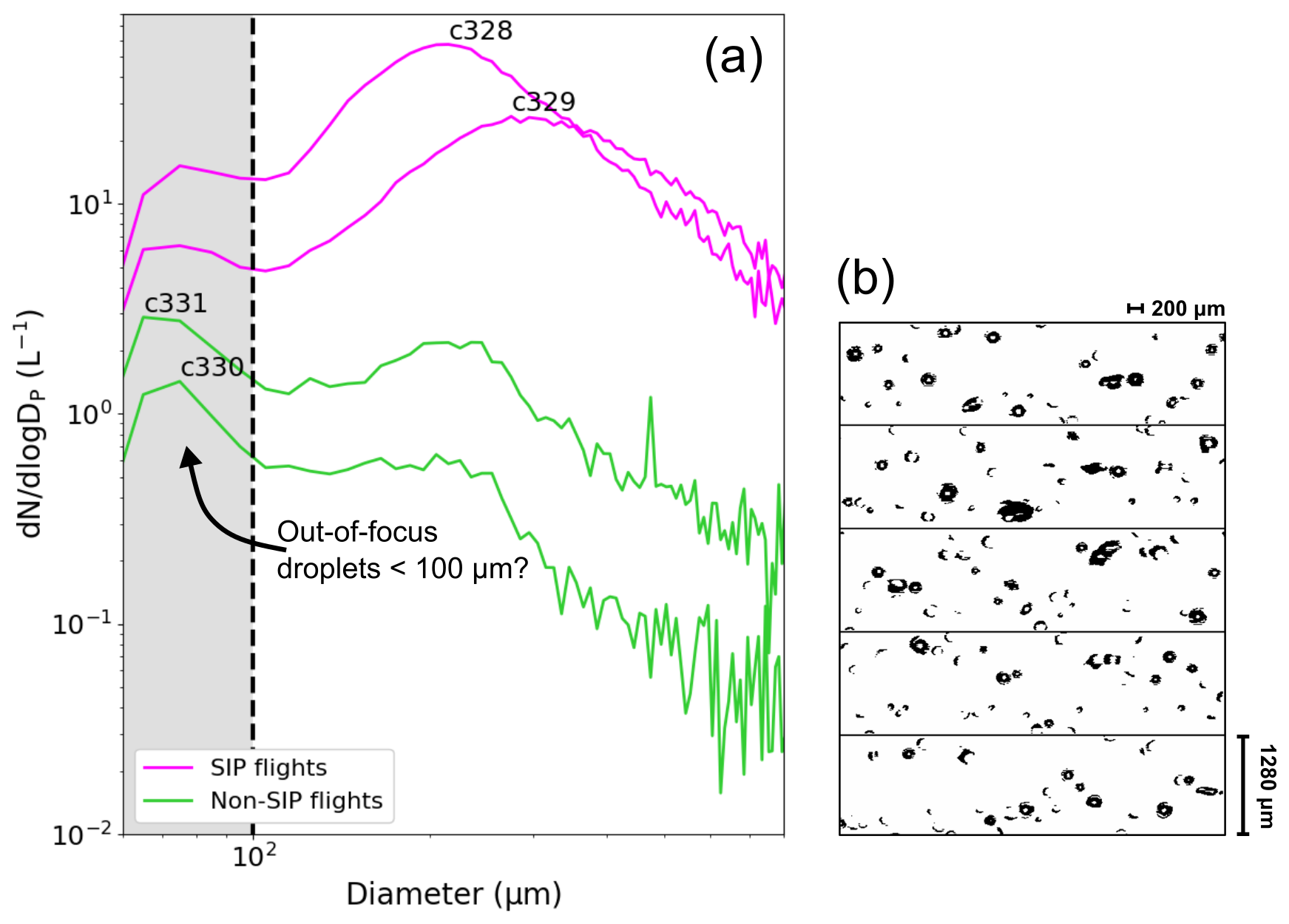
Figure A1 (a) Mean 2D-S highly irregular particle size distributions for flights C328 and C329 (pink lines), which captured strong evidence of active SIP, and flights C330 and C331 (green lines), which showed negligible evidence of ice multiplication. (b) 2D-S highly irregular particle images containing out-of-focus droplets of size < 100 µm from flight C330.

Appendix B

CAO Index

The marine CAO index (M) was calculated, following work by Fletcher et al. (2016b), to identify the M-Phase flights that successfully captured north-westerly CAO flow (Fig. 1; Table 1). Fletcher et al. (2016b) developed an index based on the difference between the potential temperatures of the surface skin (θ_SKT), describing the theoretical temperature of the uppermost surface layer which has no heat capacity and so can respond immediately to surface flux changes, and at 800 hPa (θ₈₀₀), defined as:

$$\begin{array}{}\text{(B1)}& M={\mathit{\theta }}_{\mathrm{SKT}}-{\mathit{\theta }}_{\mathrm{800}},\end{array}$$

where positive M values have been found to reliably identify the large air-sea temperature difference, and thus strong lower tropospheric instability and turbulent heat fluxes, characteristic of marine CAOs (Kolstad et al., 2009; Papritz et al., 2015; Fletcher et al., 2016a). Kolstad et al. (2009) found that using the surface skin temperature, instead of the sea surface temperature, prevents erroneous identification of CAOs in regions where sea ice cover dominates.

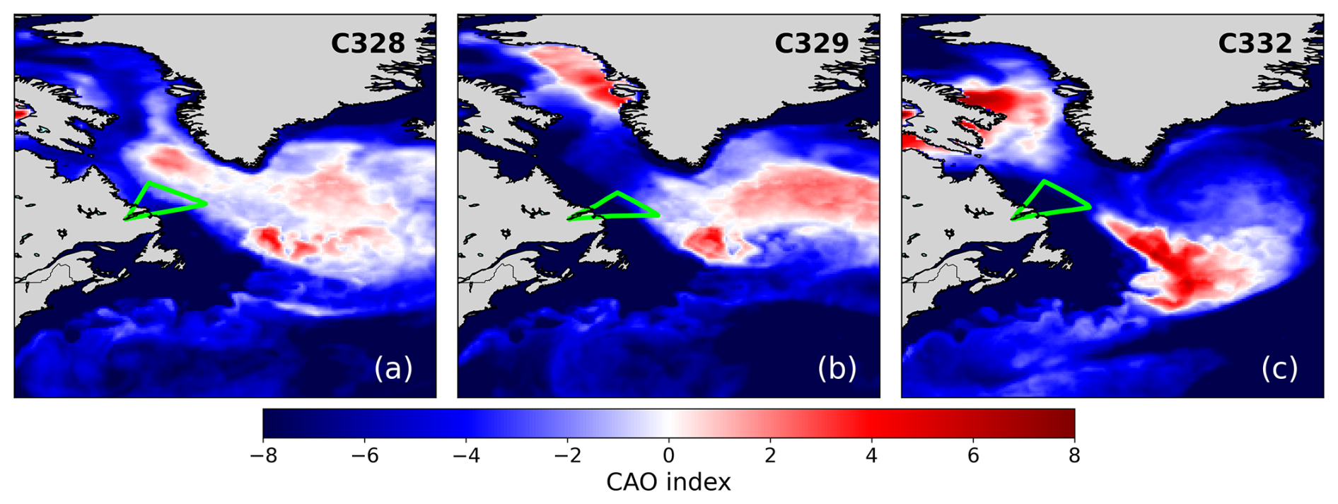
Figure B1 Mean CAO index values during M-Phase flights (a) C328, (b) C329, and (c) C332. Red and blue regions represent positive and negative index values, respectively. Flight tracks are overlaid (green lines).

To calculate M, we used skin temperature and 800 hPa air temperature output from the European Centre for Medium-Range Weather Forecasts (ECMWF) Reanalysis v5 (ERA5) from October and November 2022. The ERA5 data is available hourly on a regular latitude-longitude grid at 31 km resolution. The potential temperatures in Eq. (B1) were calculated using a standard reference pressure of 1000 hPa.

Figure B1 presents maps of mean M values calculated for the time periods coinciding with flights C328, C329 and C332, with flight tracks overlaid. In each case the cloud sampling flight legs are located in the vicinity of positive index values, which span regions correlating with the CAO regime transition to convective cloud, as shown in the satellite imagery in Fig. 2. The collocation of large, positive index values (> 2) and cumuliform cloud agrees with previous work attributing the stratiform-to-convective cloud transition to boundary layer deepening and subsequent decoupling from the sea surface as turbulent heat fluxes increase downwind with the advection of cold, polar air over warmer ocean to the south (Abel et al., 2017; Tornow et al., 2021).

Appendix C

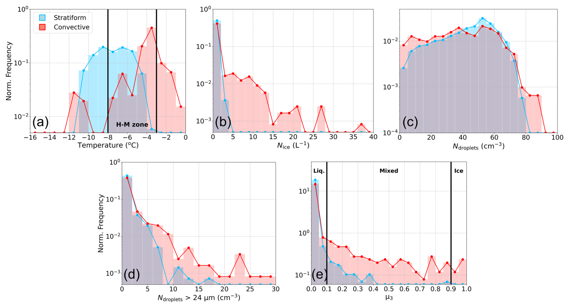
Figure C1 Relative frequency histograms of cloud microphysical properties (1 Hz data) measured within the stratiform (blue) and convective (red) regimes during flights C322 and C323, including (a) local in-cloud temperature (H–M zone marked), (b) ice crystal number concentration (N_ice), (c) total cloud droplet concentration (N_droplets), (d) concentration of cloud droplets with diameter > 24 µm, and (e) ice mass fraction (μ₃) with thresholds for liquid, mixed and ice phase cloud regions marked. Panels (b) to (e) only include data coinciding with in-cloud temperatures within H–M range (−3 to −8 °C). Data is normalised so that area under both stratiform and convective histograms integrates to 1.

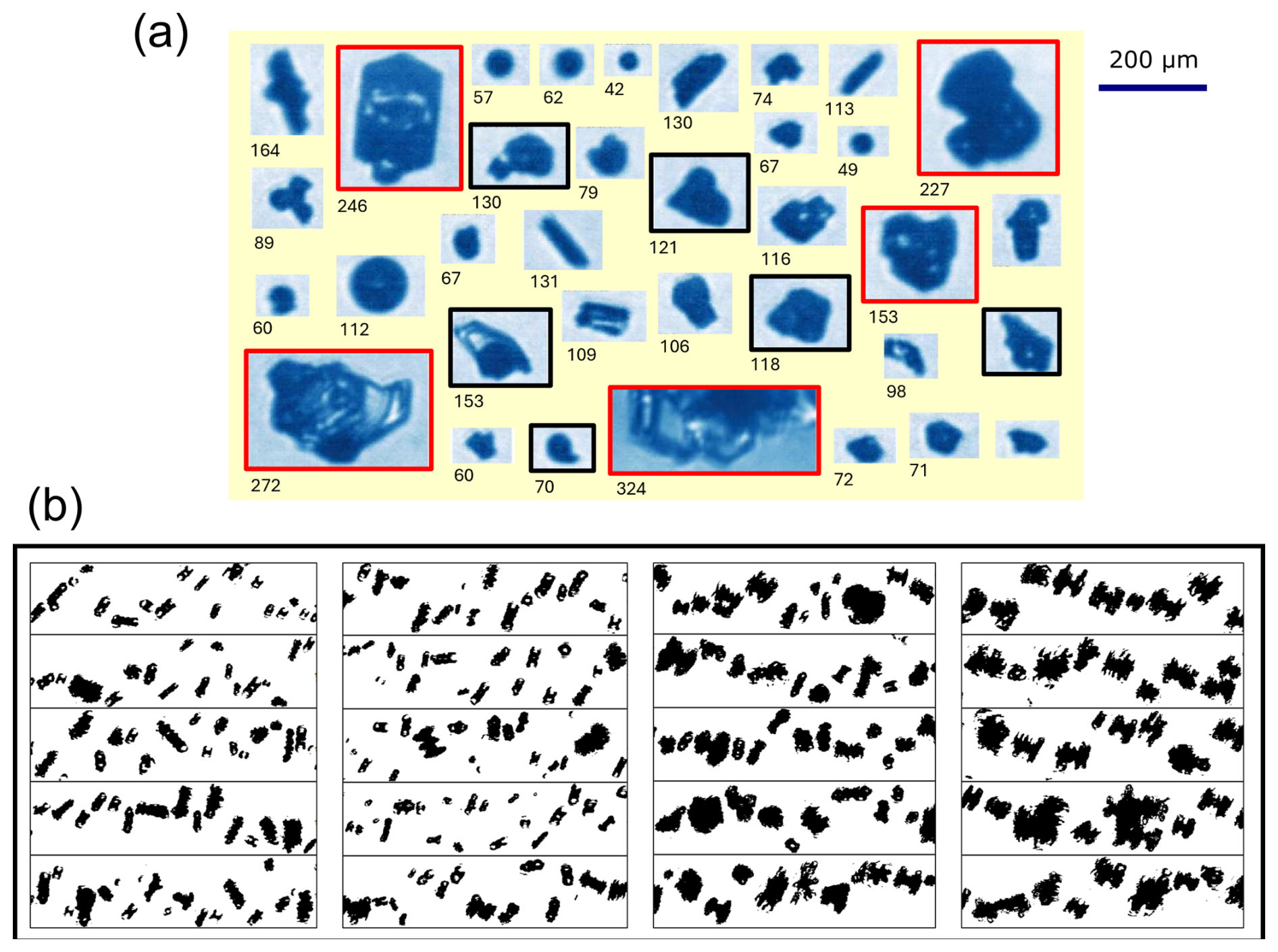
Figure C2 (a) Examples of cloud particles (ice crystals and liquid droplets) imaged with the CPI probe in SIP period 2 (between 16:19:45 and 16:20:30 UTC) during flight C328 (31 October 2022); subsets of plate-like crystals (red frames), and possible frozen droplets and fragments of shattered droplets (black frames) are highlighted; numbers below images indicate the maximum dimension length (D_p) of each particle. (b) 2D-S images of highly irregular particles captured in SIP 2; the height of each strip corresponds to the 2D-S array width of 1280 µm.

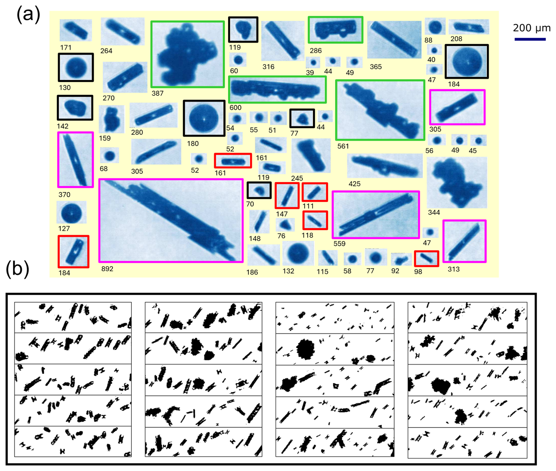
Figure C3 (a) Examples of cloud particles (ice crystals and liquid droplets) imaged with the CPI probe in SIP period 4 (between 14:11:25 and 14:13:03 UTC) during flight C329 (1 November 2022); subsets of small columnar ice of size < 200 µm (red frames), long columns (pink frames), rimed columns (green frames), and possible frozen droplets and fragments of shattered droplets (black frames) are highlighted; numbers below images indicate the maximum dimension length (D_p) of each particle. (b) 2D-S images of highly irregular particles captured in SIP 4; the height of each strip corresponds to the 2D-S array width of 1280 µm.

Appendix D

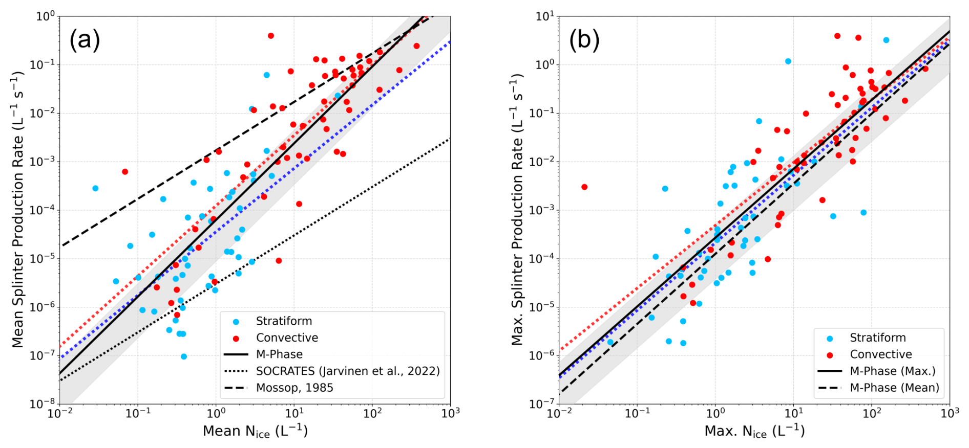
Figure D1 (a) Mean splinter production rate $\left(\frac{\mathrm{d}{N}_{\mathrm{ice}}}{\mathrm{d}t}\right)$, calculated following Willis and Hallett (1991), as a function of mean measured ice particle concentrations (including particles with D_p < 100 µm) for individual stratiform (blue) and convective (red) cloud segments with in-cloud temperatures within the H–M range of −3 to −8 °C. The solid black line represents the fit through the M-Phase data; the shaded region covers the area between fitting functions determined from maximum and minimum splinter production rates based on the overall relative uncertainty of ±86 %. The dashed and dotted black lines represent the relationships estimated by Mossop (1985c) (wintertime cumulus clouds over Australia) and Järvinen et al. (2022) (summertime CAO clouds over Southern Ocean), respectively. (b) Maximum splinter production rate $\left(\frac{\mathrm{d}{N}_{\mathrm{ice}}}{\mathrm{d}t}\right)$ as a function of maximum measured ice particle concentrations. The solid black line represents the fit through the data shown here (maximum N_ice vs. maximum splinter production rate) for all cloud segments; the dashed black line shows the fit through the data for mean cloud segment values as shown in Fig. 13.

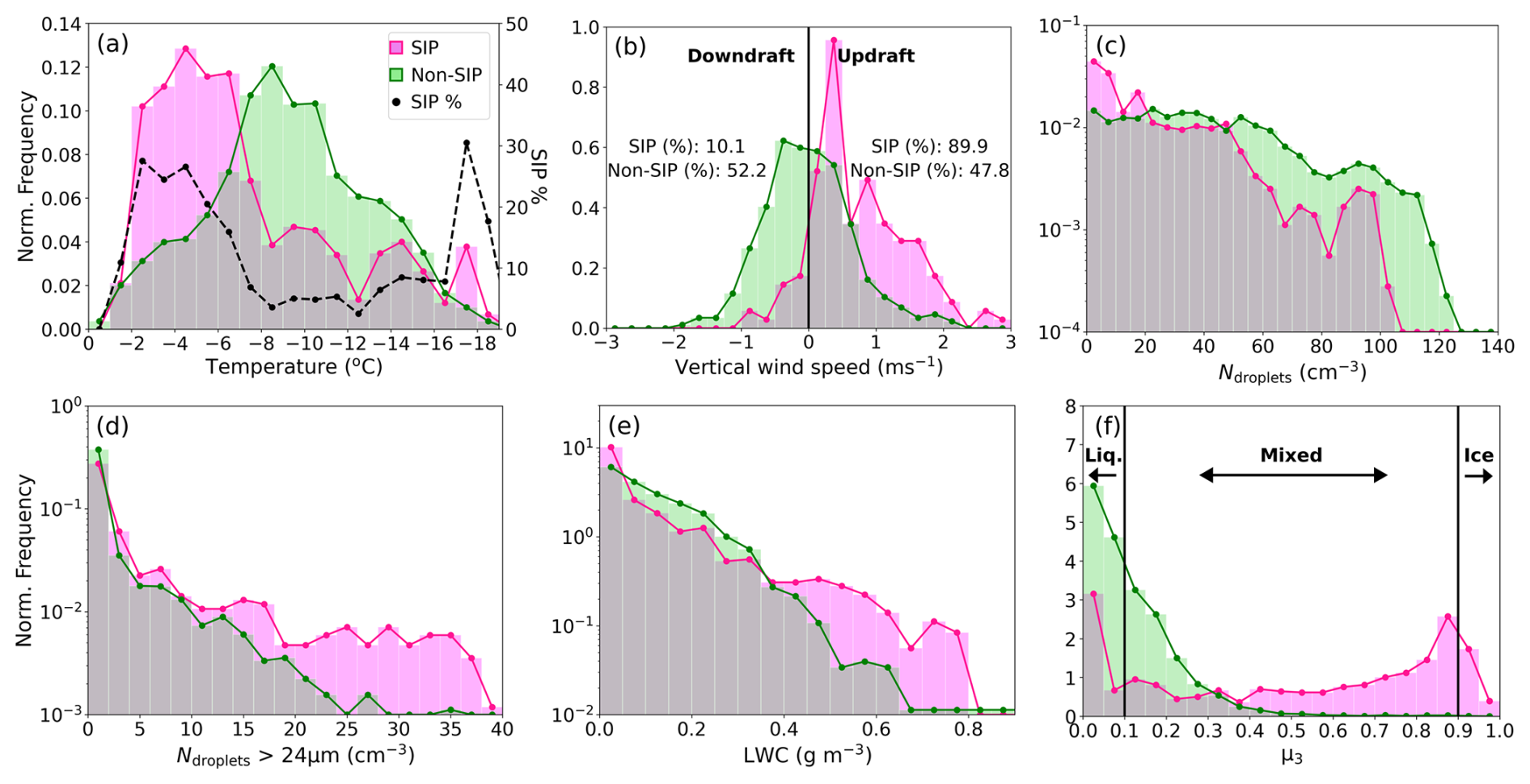
Figure D2 Relative frequency histograms of cloud microphysical properties (1 Hz data) measured within cloud regions containing strong evidence of active ice multiplication (SIP; pink), and those containing negligible evidence of active SIP processes (Non-SIP; green), including (a) local in-cloud temperature (percentage of total observations made during SIP periods within each 1 °C temperature bin also marked with dashed black line), (b) vertical wind speed (straight-and-level runs only), (c) total cloud droplet concentration, (d) concentration of cloud droplets with diameter > 24 µm, (e) liquid water content (LWC), and (f) ice mass fraction (μ₃) with thresholds for liquid, mixed and ice phase cloud regions marked. Panels (b) to (f) only include data coinciding with in-cloud temperatures within H–M range (−3 to −8 °C). Data normalised so that area under both SIP and Non-SIP histograms integrates to 1.