Consistency between zonal mean stratospheric and total column ozone trends (2000–2024)

This study presents an updated assessment of stratospheric and total column ozone trends over the 2000–2024 period using six merged limb-profile datasets and six merged total ozone datasets. Long-term changes were quantified using a multiple linear regression framework that accounts for dynamical and chemical variability. In addition to standard regressors (solar cycle, QBO, ENSO, stratospheric aerosol optical depth), we include Arctic and Antarctic Oscillation indices and the eddy heat flux in each hemisphere as proxies for dynamic variability. Volcanic (and wildfire) aerosol forcing is represented by separate proxies for three periods dominated by the major volcanic events of El Chichón, Pinatubo, and post-2000 volcanic eruptions, including Hunga-Tonga. These period-specific proxies are employed to better account for varying dynamical ozone responses that largely depend on the season and location of the eruptions. All profile datasets consistently show positive trends in the upper stratosphere, with the strongest ozone recovery in southern mid-latitudes, in agreement with other studies. In the lower stratosphere, trends remain weak, spatially heterogeneous, and predominantly negative. A comparison of stratospheric column trends derived from profile data with total ozone trends shows close agreement across all latitude bands. Within the trend uncertainties, total column trends since 2000 are largely driven by stratospheric ozone changes, while tropospheric contributions to zonal-mean total ozone trends (the difference between total and stratospheric column trends) appear negligible. The extended regression framework improves the representation of recent dynamical variability and provides an updated perspective on stratospheric ozone recovery through 2024.

1 Introduction

The stratospheric ozone layer absorbs the sun's ultraviolet radiation, which is harmful to humans and the planet's environment (e.g. Bornman et al., 2023). With the depletion of global stratospheric ozone through the 1990s due to ozone-depleting substances (ODS) (Solomon, 1999), the ozone layer was significantly weakened, especially in the polar regions during spring, leading to the development of the Antarctic ozone hole (Farman et al., 1985). The enactment of the Montreal Protocol in 1987 and its Amendments phased out ODS to counteract this decrease in ozone (Velders et al., 2007; WMO, 2018). A slow but gradual ozone recovery on the order of 1 % per decade to 2 % per decade above around 35 km in the upper stratosphere is evident (e.g. Steinbrecht et al., 2017; Sofieva et al., 2017, 2023; Ball et al., 2018; Arosio et al., 2019; Petropavlovskikh et al., 2019; Szeląg et al., 2020; Li et al., 2023), coinciding with the decline of stratospheric halogens released from the ODS (Bernath and Fernando, 2018; Steffen et al., 2019; Froidevaux et al., 2022). The upper stratospheric trends remain robust and nearly unchanged after ozone timeseries updates to the end of 2024 (Sofieva et al., 2026).

In addition to ODS, atmospheric dynamics and changes in greenhouse gases also significantly influence ozone, particularly, in the lower stratosphere (Chipperfield et al., 2015; WMO, 2022). Ozone trends in the lower stratosphere are in some cases negative but have larger uncertainties and are often not statistically different from zero (Godin-Beekmann et al., 2022), although statistically significant trends have been reported in some studies. Ball et al. (2018, 2019) reported negative trends ranging from the tropics to mid-latitudes. Most chemistry-climate models predict ozone decreases in the tropical lower stratosphere and increases in the extratropics due to a strengthening of the Brewer-Dobson circulation in a changing climate (e.g. Ball et al., 2020), which is in contradiction to Ball et al. (2018, 2019) showing negative trends in the extratropics. Since total ozone trends show negligible trends in the tropics (Weber et al., 2022), it was hypothesised that increases in tropical tropospheric ozone may have balanced decreases in the lower stratosphere (Ball et al., 2018).

Because of the rather limited lifetime of individual satellite missions (up to a maximum of 20 years), merged ozone datasets are needed to analyse ozone trends over several decades. These datasets are the combination of multiple satellite measurements of ozone profiles merged into a single 40+ year coherent dataset. In this study, we use a multiple linear regression (MLR) and apply it to six long-term ozone profile datasets and six long-term total ozone datasets to analyze ozone variability and trends over the time period from 2000 to 2024.

In previous multiple linear regression (MLR) studies of total ozone trends additional dynamical proxies, like the Arctic and Antarctic Oscillation (AO/AAO) and hemispheric eddy heat fluxes representing the Brewer-Dobson circulation, were needed to properly model the strong variability in extratropical total ozone (Chehade et al., 2014; Weber et al., 2018, 2022). These dynamical proxies were not used in the most comprehensive and recent ozone profile trend studies by Godin-Beekmann et al. (2022) and Sofieva et al. (2026). Both studies use the so-called LOTUS model setup (Petropavlovskikh et al., 2019), which includes proxies for Quasi-Biennial Oscillation (QBO), 11-year solar cycle, El Niño-Southern Oscillation (ENSO), and stratospheric aerosols.

Applying the same MLR settings to both total column and vertical profile data shall allow us to answer the question of how much stratospheric and total column trends differ, providing some estimates of the tropospheric contributions (i.e. the differences between total and stratospheric column trends).

The major objective of this study is to assess post-2000 ozone trends through 2024 using multiple independent merged profile and total column datasets. While continued upper-stratospheric recovery has been recently confirmed (Sofieva et al., 2026), the magnitude and hemispheric structure of post-2000 trends, particularly in the lower stratosphere and polar regions, remain sensitive to methodological choice in the MLR setup, including proxy selection and treatment of volcanic forcing. Lower stratospheric (around 5 km above the tropopause) ozone has the largest contribution to total column ozone.

By comparing standard regression configurations like the LOTUS setup with an extended proxy setup that explicitly represents dynamical variability (AO, AAO, and eddy heat flux) and separates major volcanic aerosol periods, including the latest period that is dominated by the Hunga Tonga-Hunga Ha'apai (HTHH) volcanic event, we evaluate the relative contributions of stratospheric versus tropospheric changes to total column trends. Our approach allows us to distinguish chemically driven long-term recovery from dynamically induced variability and trends, acknowledging that chemistry–dynamics coupling may limit a strict separation.

This paper is structured as follows. Section 2 summarises briefly the details on the merged ozone datasets. Section 3 describes the conversion of some of the profile data to a common altitude grid (geometric altitude) and ozone units (number density). The unit conversions are necessary for calculating stratospheric columns from the ozone profiles. Uncertainties arising from the conversion are assessed. In addition, the long-term drifts between the datasets are investigated. Section 4 summarises the MLR setup and the proxy settings. Results are reported in Sect. 5, followed by a discussion (Sect. 6) and summary (Sect. 7).

2 Data

To ensure a consistent analysis of long-term ozone trends, this study uses a harmonized (common altitude and ozone unit) set of monthly mean datasets (Tables 1, A1). Both vertically resolved ozone profile data and total column ozone datasets are included to provide a comprehensive picture of ozone trends. Since the individual profile datasets differ in their vertical and latitudinal grids, as well as in ozone units, all ozone monthly mean profiles are converted to common grids and units before further analysis. Reanalysis data from ERA5 and reference measurements from Aura MLS are used to perform and evaluate these conversions, respectively, ensuring internal consistency across datasets.

2.1 Ozone profile datasets

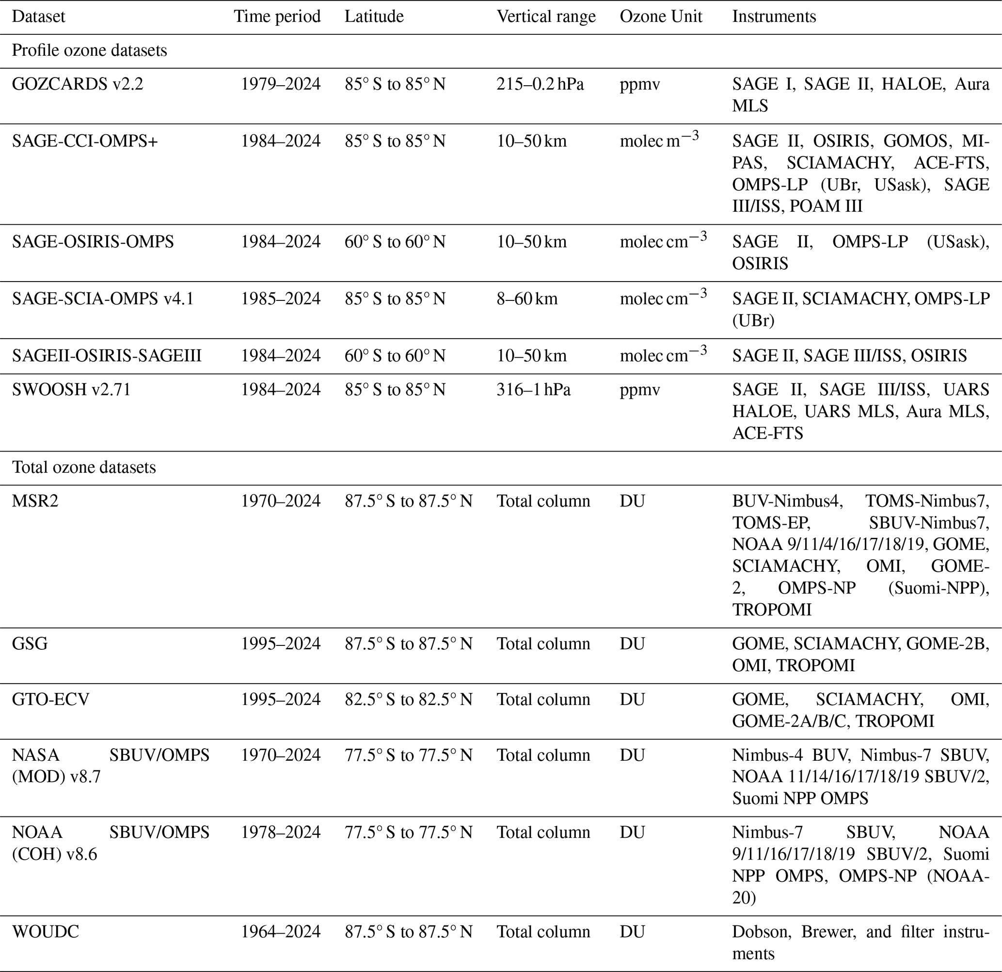
This study uses six long-term merged limb satellite ozone profile datasets: GOZCARDS (Global OZone Chemistry And Related trace gas Data records for the Stratosphere), SAGE-CCI-OMPS (SAGE II, Climate Change Initiative and OMPS), SAGE-OSIRIS-OMPS (SAGE II, OSIRIS and OMPS), SAGEII-OSIRIS-SAGEIII (SAGE II, OSIRIS and SAGE III), SAGE-SCIA-OMPS (SAGE II, SCIAMACHY and OMPS), and SWOOSH (The Stratospheric Water and Ozone Satellite Homogenized). All datasets provide monthly zonal mean stratospheric ozone profiles and are widely used for long-term trend analyses (e.g. Steinbrecht et al., 2017; Godin-Beekmann et al., 2022; Sofieva et al., 2023, 2026). Most datasets begin in 1984/1985 with the launch of SAGE-II, while GOZCARDS extends back to 1979, providing the longest record. All datasets are extended until the end of 2024, enabling consistent post-2000 trend analyses. The temporal coverage of contributing instruments is shown in Fig. 1, and dataset characteristics including latitude coverage, vertical range, ozone units, while contributing instruments are summarized in Table 1. The datasets employ different merging strategies, including anomaly-based merging, debiased absolute-value merging, and absolute-value merging with retained seasonal structure. Despite these methodological differences, all datasets are internally consistent, quality-controlled, and suitable for assessing long-term stratospheric ozone trends. For consistency, all ozone profile datasets are converted to a common latitude–altitude grid and unified ozone units (Sect. 3.1). A more detailed description of the datasets is given by Steinbrecht et al. (2017) and Davis et al. (2026).

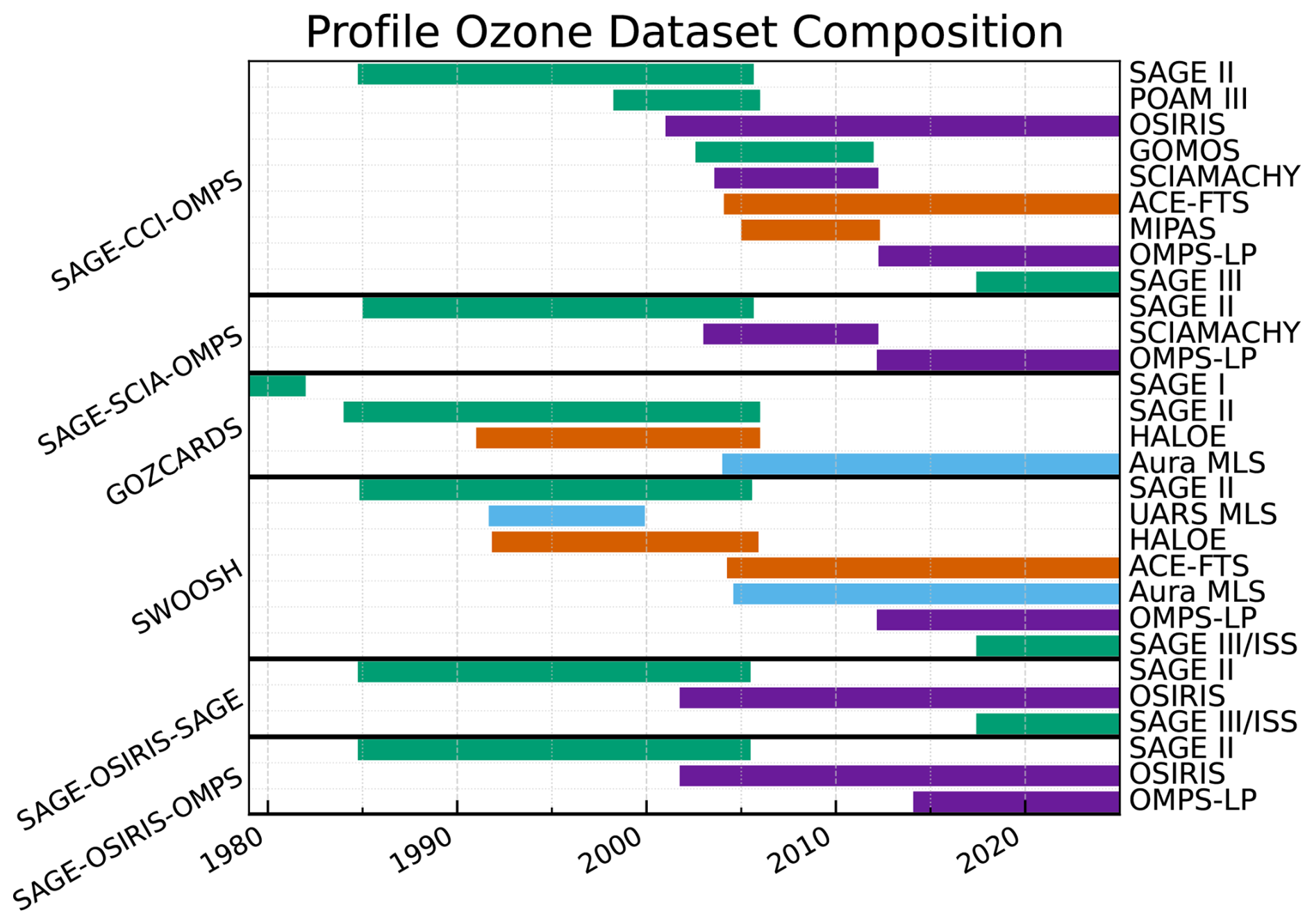
Figure 1 Satellite missions contributing to each of the six merged ozone profile datasets. The instruments shown in light blue measure in the microwave region, those shown in green measure in the UV/visible region, those shown in orange measure in the thermal infrared region, and those shown in violet measure UV/visible limb scatter.

2.2 Total ozone datasets

Six long-term merged total column ozone datasets: MSR2 (Multi-sensor re-analysis), GSG (GOME/SCIAMACHY/GOME2), GTO-ECV (GOME-type Total Ozone – Essential Climate Variable), SBUV (Solar Backscatter Ultraviolet) NASA (MOD (Merged Ozone Data Set)), SBUV NOAA (COH (Cohesive)), and WOUDC (World Ozone and Ultraviolet Radiation Data Centre) are analysed. All datasets extend through the end of 2024 and provide quality-controlled estimates of total ozone suitable for long-term trend analysis. The zonal mean total ozone records generally begin earlier than the profile datasets, with start dates from 1960 (WOUDC) and 1970 (SBUV-MOD). SBUV-COH starts in 1978, while GTO-ECV and GSG start in 1995. In the MLR, the latter two datasets are extended back in time to 1978, the starting year of the regression, using the SBUV-COH data (Weber et al., 2022). The temporal coverage, latitudinal range, and contributing instruments of each dataset are summarized in Table 1, while the contribution of individual instruments is illustrated in Fig. 2.

The datasets comprise a mix of satellite-only merged products and one dataset based upon ground-based observations (WOUDC). The MSR2 dataset provides globally gridded total ozone fields based on data assimilation using individual data records that are bias corrected using ground-based data from Brewer and Dobson instruments (van der A et al., 2015). The remaining satellite products apply homogenization and bias-corrections to match individual data records. WOUDC complements the satellite records by providing zonal mean data derived from ground-based total ozone measurements from Dobson, Brewer, and filter instruments. Zonal mean ground data are calculated combining station data and an ozone climatology (Fioletov et al., 2002, 2008). More details on the various merged datasets can be found in Weber et al. (2022) and Davis et al. (2026).

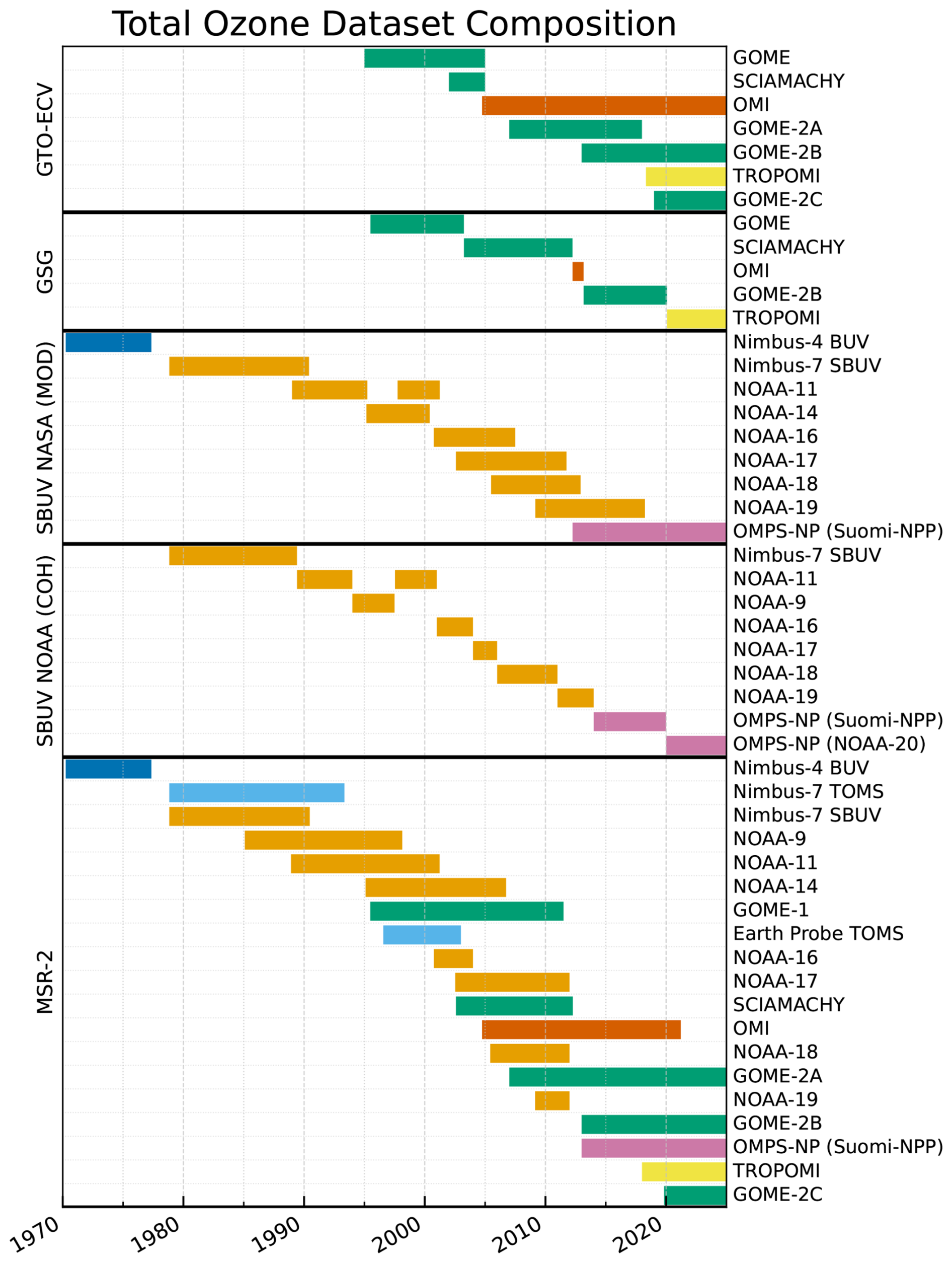
Figure 2 Same as Fig. 1, but for the six merged total ozone datasets. The colors indicate the different instrument families.

Table 1 Overview of merged ozone datasets used in this study, including their temporal coverage, spatial resolution, and original ozone units.

2.3 Auxilliary datasets used for assessing uncertainties in unit conversion

In this study, all ozone profile datasets are expressed in units of number densities [molec cm⁻³] as a function of geometrical altitude [km]. This conversion is needed to directly compare the ozone trends in absolute units and will help in calculating the stratospheric column. The conversion was applied to GOZCARDS and SWOOSH (see Table A1). Meteorological data (geopotential height, pressure, and temperature) from the ERA5 re-analysis data were used for the conversion of the datasets (Hersbach et al., 2020). Apart from the uncertainties in reanalysis temperatures, the conversion applied to monthly mean data, as provided in the merged data product, may lead to uncertainties compared to a merged data product based upon single ozone profiles converted before calculating the monthly means. The conversion of individual ozone profiles before averaging, gridding, and merging is considered to be more accurate, but is not possible if monthly mean merged data sets are used. We quantify this additional uncertainty using Aura MLS (Microwave Limb Sounder) ozone and temperature observations.

MLS, aboard NASA's Aura satellite, provides high vertical resolution ozone profiles spanning from the upper troposphere into the mesosphere (Waters et al., 2006). The long-term stability of Aura MLS has been assessed in comparisons to ground-based data (e.g. Hubert et al., 2016) and MLS is, therefore, suitable for assessing the conversion uncertainty.

3 Data Preparation

3.1 Ozone unit and vertical grid conversion

The limb ozone profile merged datasets (Table 1) are level 3 (L3) monthly mean zonal mean datasets having different ozone units, vertical grids, and spatial resolutions. For a direct comparison of the profile ozone trends, we convert the datasets to common ozone units and vertical grid and re-bin them to a common spatial grid. The advantage of using number density and geometric altitude is the calculation of partial ozone column amounts (e.g. stratospheric) by simple vertical integration of the ozone profile. The units and altitude grid conversion are only needed for SWOOSH and GOZCARDS.

The common latitude grid is defined by the lowest available resolution of the profile datasets, which ranges from 85° S to 85° N (center latitudes) in 10° steps. The merged ozone datasets were created from level-2 (L2) orbit data. The unit conversion of the monthly mean L3, as done in this work, instead of L2 data, may contribute to trend uncertainties. To evaluate the impact of this conversion, we compared two conversion approaches using the MLS/Aura L2 data (2004–2022). The first approach converts the MLS L2 individual profiles to the common ozone and altitude units and afterward creates the monthly mean L3 data. The second approach first determines the L3 data and then applies the unit conversion to the monthly mean L3 data using monthly mean zonal mean meteorological parameters: temperature, pressure, and altitude from ERA5. The linear trends of the difference timeseries between both approaches give an estimate of the trend uncertainty resulting from the unit conversion.

Figure 3 shows the trend of the difference timeseries between both approaches as a function of latitude and month for selected altitude levels. Most of the trends are not significant (hatched areas). At 25 km, a negative trend of around 1 % per decade between April and August in the northern hemisphere (NH) and between January and July in the southern hemisphere (SH) is noted. The significance of these trends decreases with altitude, showing the most significant trends at 25 km. This is possibly because of stronger vertical ozone or temperature gradients near this altitude, which increase the uncertainties from the non-linear ozone unit conversion and vertical axis transformation. Especially in the SH, insignificant trends are observed at higher altitudes (40 km). In general, we conclude that the trend uncertainty due to unit and altitude grid conversions is small and insignificant, but in selected regions and months non-negligible.

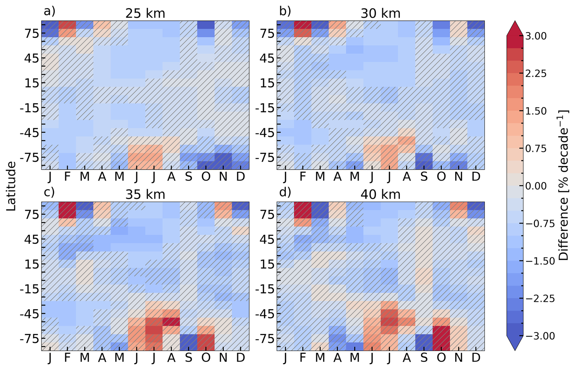
Figure 3 Zonal mean decadal trends of differences between MLS L3 data converted after and before gridding (post-gridded – pre-gridded) in % per decade from 2005 to 2022 at altitudes of 25, 30, 35 and 40 km (panels a–d). Hatches indicate insignificant trends within 2σ.

3.2 Relative Drifts among Multiple Datasets

Another contribution to uncertainties in long-term trends arises from relative drifts among the merged datasets. Here, relative drifts refer to systematic long-term differences between individual datasets and a common reference, in this case the multi-instrument mean (MIM). The spread of the drifts provides an estimate for possible contribution to trend uncertainties derived from multiple datasets.

To assess these relative drifts, a simple linear regression is applied to the time series of differences between the monthly mean merged datasets and the MIM. The percentage ozone difference timeseries is calculated as follows for each profile dataset:

$$\begin{array}{}\text{(1)}& {\displaystyle }\mathrm{\Delta }{O}_{\mathrm{3}}(z,t)=\mathrm{100}\cdot {\displaystyle \frac{O_{\mathrm{3}}(z,t)-\text{MIM}(z,t)}{\text{MIM}(z,t)}},\end{array}$$

where O₃ is the ozone concentration of the merged dataset (in number density or DU). The linear trend (or relative drift) of the ΔO₃ timeseries from all datasets is computed, and the standard deviation of the mean of these trends represents the 1σ drift uncertainty, which is independent of the common reference, here MIM.

Figure 4 shows the 1σ drift uncertainty derived from the six merged profile datasets until the end of 1995 and since 2000. It ranges from 0.5 % per decade to 0.75 % per decade for the period 2000 to 2024 between 60° S and 60° N and above 20 km. The uncertainties are larger at higher latitudes and lower altitudes and are most likely due to higher uncertainties in ozone measurements. In the period between 1985 through 1995, the uncertainties show higher values from close to the tropopause up to 25 km for latitudes above 50° N $/$ 50° S. Above this altitude and in the zonal band between these latitudes, the uncertainties are comparable in magnitude with those from the later period.

The same procedure was applied to the total ozone datasets, and results are shown for the period since 1996 (ODS peak) and 2000 in Fig. 5. We did not include the period before the ODS peak in this figure, because two of the total ozone datasets start around 1995 (GTO-ECV and GSG), leaving us with a limited selection of merged datasets and instruments before that year. Instead we show the relative drift uncertainty for two different start years (1996 and 2000), which were used in previous studies (Weber et al., 2022; Godin-Beekmann et al., 2022; Sofieva et al., 2026). Both relative drift uncertainties look very similar and show no significant differences. The drift uncertainties in the period 2000–2024 are slightly larger than in the period starting in 1996. When comparing the drift uncertainty for the total ozone datasets to the profile ozone datasets (Fig. 4), we see that the total ozone dataset drifts are overall lower and range between 0.1 % per decade and 0.5 % per decade. The highest values can be seen at high latitudes and in the tropics, while the mid-latitudes show very low uncertainties. Higher drift uncertainties at higher latitudes are most probably due to the combination of higher uncertainties in ozone itself (higher solar zenith angles) and a larger natural variability in ozone. It is not clear why the drift uncertainties are enhanced in the tropics. Probably the low natural ozone variability masks the drifts to a lesser degree.

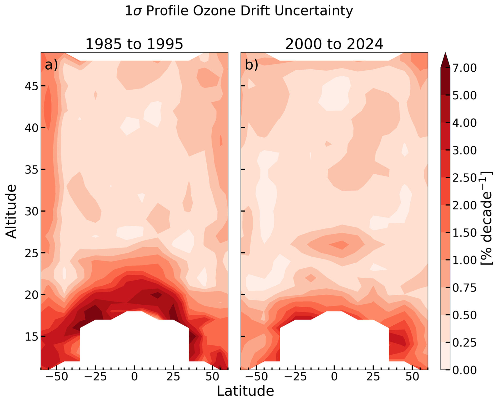
Figure 4 Standard deviation (1σ) of the drifts relative to the multi-instrument mean derived from GOZCARDS, SAGE-CCI-OMPS, SAGE-SCIA-OMPS, SAGE-OSIRIS-OMPS, SAGEII-OSIRIS-SAGEIII and SWOOSH profile data for the periods (a) 1985 to 1995 and (b) 2000 to 2024 as a function of latitude and altitude.

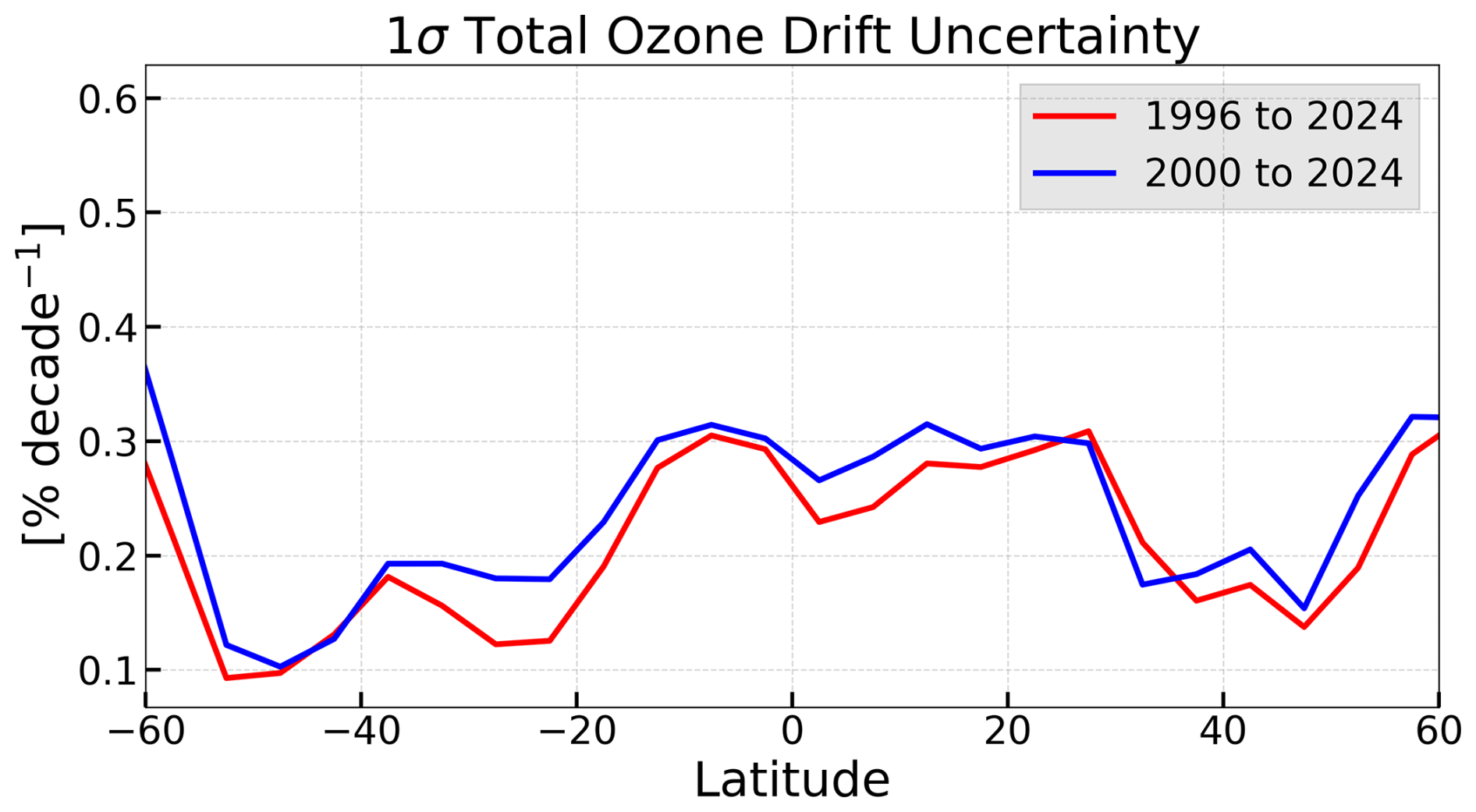
Figure 5 Standard deviation (1σ) of the mean of the drifts (1σ) derived from NASA SBUV, NOAA SBUV, GSG, GTO-ECV, and MSR2 total column data since 1996 (red line) and 2000 (blue line) as a function of latitude.

4 Methods

4.1 Trend analyses

We apply a multiple linear regression (MLR) model to time series of ozone at each altitude-latitude grid point (for profile data) and each latitude (for total column data) including terms that account for various atmospheric processes, e.g. solar cyle, QBO, and El-Nino. The following equation shows the MLR equation (Godin-Beekmann et al., 2022; Sofieva et al., 2026) with additional proxies (see Table 2) as used in this study:

$$\begin{array}{}\text{(2)}& \begin{array}{rl}{\displaystyle }y(z,t)& {\displaystyle }={\mathit{\beta }}_{\mathrm{1}}(z,t)\cdot {\text{QBO}}_{\mathrm{1}}\left(t\right)+{\mathit{\beta }}_{\mathrm{2}}(z,t)\cdot {\text{QBO}}_{\mathrm{2}}\left(t\right)\\ {\displaystyle }& {\displaystyle }+{\mathit{\beta }}_{\mathrm{3}}(z,t)\cdot \text{ENSO}\left(t\right)+{\mathit{\beta }}_{\mathrm{4}}(z,t)\cdot \text{Solar}\left(t\right)\\ {\displaystyle }& {\displaystyle }+{\mathit{\beta }}_{\mathrm{5}}(z,t)\cdot {\text{SAOD}}_{\text{ElChichon}}\left(t\right)+{\mathit{\beta }}_{\mathrm{6}}(z,t)\\ {\displaystyle }& {\displaystyle }\cdot {\text{SAOD}}_{\text{Pinatubo}}\left(t\right)+{\mathit{\beta }}_{\mathrm{7}}(z,t)\cdot {\text{SAOD}}_{\text{HTHH}}\left(t\right)\\ {\displaystyle }& {\displaystyle }+{\mathit{\beta }}_{\mathrm{8}}(z,t)\cdot \text{AO}\left(t\right)+{\mathit{\beta }}_{\mathrm{9}}(z,t)\cdot \text{AAO}\left(t\right)+{\mathit{\beta }}_{\mathrm{10}}(z,t)\\ {\displaystyle }& {\displaystyle }\cdot \text{EHFS}\left(t\right)+{\mathit{\beta }}_{\mathrm{11}}(z,t)\cdot \text{EHFN}\left(t\right)\\ {\displaystyle }& {\displaystyle }+\left({\mathit{\beta }}_{\mathrm{12}}\right(z,t)+{\mathit{\beta }}_{\mathrm{13}}(z,t\left)\right(t-t_{\mathrm{0}}\left)\right)\cdot L_{\text{pre}}\left(t\right)\\ {\displaystyle }& {\displaystyle }+{\mathit{\beta }}_{\mathrm{14}}(z,t)\cdot L_{\text{Gap}}\left(t\right)+\left({\mathit{\beta }}_{\mathrm{15}}\right(z,t)+{\mathit{\beta }}_{\mathrm{16}}(z,t\left)\right(t-t_{\mathrm{1}}\left)\right)\\ {\displaystyle }& {\displaystyle }\cdot L_{\text{post}}\left(t\right)+\mathit{\epsilon }(z,t)\end{array}\end{array}$$

with y(z,t) being the monthly mean ozone as a function of altitude z and running month t and β_k the regression coefficients.

Terms containing L_pre, L_Gap(t), and L_post cover only consecutive periods with separate linear trend coefficients, β₁₃ and β₁₆, before and after the ODS peak in 1996, respectively. These three variables are defined as follows:

$$\begin{array}{}\text{(3)}& L_{\text{pre}}\left(t\right)=\left\{\begin{array}{ll}\mathrm{1}& \text{if }t<t_{\mathrm{0}}\\ \mathrm{0}& \text{if }t\ge t_{\mathrm{0}}\end{array}\right.,\end{array}$$

$$\begin{array}{}\text{(4)}& L_{\text{Gap}}\left(t\right)=\left\{\begin{array}{ll}\mathrm{0}& \text{if }t<t_{\mathrm{0}}\text{ and }t\ge t_{\mathrm{1}}\\ \mathrm{1}& \text{if }{t}_{\mathrm{0}}\le t<t_{\mathrm{1}}\end{array}\right.,\end{array}$$

and

$$\begin{array}{}\text{(5)}& L_{\text{post}}\left(t\right)=\left\{\begin{array}{ll}\mathrm{0}& \text{if }t<t_{\mathrm{1}}\\ \mathrm{1}& \text{if }t\ge t_{\mathrm{1}}\end{array}\right..\end{array}$$

t₀ is January 1996 and t₁, December 1999. Note that the term with L_Gap(t) does not contain a linear trend coefficient during the gap period (1996–1999). This is needed to reduce the influence of the selection of a turnaround point between ozone decline and recovery because the timing of the trend reversal varies with latitude and altitude (Laine et al., 2014). By introducing a transition period rather than a single inflection year, the regression model allows for a more gradual change between the two trend segments.

To consider seasonality more explicitly, the regression model uses harmonic terms to represent the annual and semi-annual cycles of selected terms, as shown in Eq. (6).

$$\begin{array}{}\text{(6)}& \begin{array}{rl}{\mathit{\beta }}_k(z,t)& ={\mathit{\beta }}_{k\mathrm{0}}\left(z\right)+\sum _{i=\mathrm{1}}^{\mathrm{2}}\left[{\mathit{\beta }}_{k\mathrm{1}i}\left(z\right)\sin \left({\displaystyle \frac{\mathrm{2}\mathit{\pi }it}{\mathrm{12}}}\right)\right.\\ & \left.+{\mathit{\beta }}_{k\mathrm{2}i}\left(z\right)\cos \left({\displaystyle \frac{\mathrm{2}\mathit{\pi }it}{\mathrm{12}}}\right)\right].\end{array}\end{array}$$

Harmonic terms are only used for the QBO, ENSO, and fit coefficients in the trend terms (β₁₂ to β₁₆). This approach is robust for non-deseasonalized data and helps reduce uncertainty in the estimated trend, particularly in datasets with sparse temporal coverage.

Trend uncertainties are derived from the covariance matrix of the regression coefficients. Since ordinary least squares assumes uncorrelated residuals, it tends to underestimate uncertainties when applied to ozone time series. To account for autocorrelation, we correct for first-order autocorrelation (AR-1) in the regression residuals (Cochrane and Orcutt, 1949). This is achieved by calculating the lag-1 autocorrelation and applying a transformation to the regression model that reduces the serial correlation of the residuals (Reinsel et al., 2002). The transformed regression equation provides the adjusted fitting coefficients and their uncertainties.

When reporting mean trends from multiple datasets, we use two different formulas for the uncertainty, explained in the LOTUS report and in more detail in Petropavlovskikh et al. (2019). For consistency with the previous analyses (Weber et al., 2022; Godin-Beekmann et al., 2022), we present both uncertainty estimates in our paper. First we use the LOTUS uncertainty estimate (Petropavlovskikh et al., 2019; Sofieva et al., 2026), which is defined as the maximum uncertainty of two terms:

$$\begin{array}{}\text{(7)}& {\mathit{\sigma }}_{\text{mean}}^{\mathrm{2}}=max\left({\displaystyle \frac{\mathrm{1}}{N^{\mathrm{2}}}}\sum _{i,j}{C}_{ij}{\mathit{\sigma }}_i{\mathit{\sigma }}_j,{\displaystyle \frac{\mathrm{1}}{n_{\text{eff}}}}\sum {\displaystyle \frac{(x_i-\overline{x}{)}^{\mathrm{2}}}{N-\mathrm{1}}}\right).\end{array}$$

The first term represents the variance of the mean of correlated trend estimates, accounting for the individual regression uncertainties and the correlations of model-data residuals. The LOTUS report uses constant correlation coefficients C_ij for the pre-1997 period and for the post-2000 period. In this paper we use latitude- and altitude-dependent correlation coefficients, which do not change the results substantially (Petropavlovskikh et al., 2019). The second term is based on the sample variance of the individual trend estimates; the effective number of independent datasets, n_eff is defined as follows:

$$\begin{array}{}\text{(8)}& n_{\text{eff}}={\displaystyle \frac{N^{\mathrm{2}}}{{\sum }_{i,j=\mathrm{1}}^N{C}_{ij}}}\end{array}$$

(Petropavlovskikh et al., 2019).

The second approach, the J-distribution, is a more conservative estimate and characterizes the total ensemble variance of trend estimates (Ko et al., 2013; Harris et al., 2015; Petropavlovskikh et al., 2019), which is defined as follows:

$$\begin{array}{}\text{(9)}& {\mathit{\sigma }}_{\text{mean}}^{\mathrm{2}}={\displaystyle \frac{\mathrm{1}}{N}}\sum {\mathit{\sigma }}_i^{\mathrm{2}}+\sum {\displaystyle \frac{(x_i-\overline{x}{)}^{\mathrm{2}}}{N-\mathrm{1}}}.\end{array}$$

The first term accounts for uncertainties in the trends of the individual datasets and the second term represents the contribution from taking the statistical mean of the individual trends. The joint distribution is considered a conservative estimate (Ko et al., 2013) and produces larger uncertainties than other methods (Steinbrecht et al., 2017; Petropavlovskikh et al., 2019). Both the LOTUS estimate (Eq. 7) and the J-distribution (Eq. 9) consist of two components: the first arises from uncertainties in the MLR fit, while the second characterizes the spread of trend estimates across datasets. However, the two approaches differ in the interpretation of these terms. The J-distribution assumes that the dominant contribution to the MLR uncertainty, estimated from fit residuals, reflects unresolved variability not captured by the trend model. As a consequence, trend estimates from different datasets are effectively treated as fully correlated with respect to this component, and averaging does not reduce this contribution. In the case of C_ij=1, the first terms in Eqs. (7) and (9) become identical. In contrast, the LOTUS estimate accounts for partial correlations between trend uncertainties, with correlation coefficients derived from fit residuals and ranging between approximately 0.6 and 0.95 for the datasets considered here. The second term in the J-distribution represents the full ensemble variance, whereas the LOTUS estimate corresponds to the standard error of the mean for correlated values. Since n_eff≈1.4 for the considered datasets, this term is only slightly reduced in the LOTUS formulation compared to the J-distribution. The J-distribution combines both contributions additively, while the LOTUS estimate uses the maximum of the two terms. For consistency with previous analyses (Weber et al., 2022; Godin-Beekmann et al., 2022), both the LOTUS and J-distribution uncertainty estimates are used in this study. A detailed comparison of the two approaches is provided in Petropavlovskikh et al. (2019).

4.2 Proxy Setup

A list of the proxies used here is given in Table 2. The proxy timeseries have been normalized to the range from −0.5 to 0.5, except for the stratospheric aerosol optical depth (SAOD) (0 to 1 range). They have not been detrended, which means the dynamics-related trends are captured by the proxies rather than by the linear trend terms. This way the linear trends approximate the long-term ODS-related ozone change (Weber et al., 2018). In contrast to the common proxy setup of the LOTUS model (Petropavlovskikh et al., 2019; Godin-Beekmann et al., 2022; Dubé et al., 2023; Sofieva et al., 2026), we add the Arctic and Antarctic Oscillation (AO/AAO), the Brewer-Dobson Circulation (BDC) as expressed by the eddy heat fluxes (EHFN, EHFS), and three separate SAOD proxies (Weber et al., 2022). Both EHFN and EHFS are proxies derived from ERA5 reanalysis ín the respective hemisphere (45–75°). The Brewer-Dobson circulation in boreal and austral winter has an ozone response in the tropics opposite to that in the extratropics (e.g. Weber et al., 2011). There is also SH ozone response to the Brewer-Dobson circulation in the NH (Fioletov and Shepherd, 2003). For this reason, EHFN and EHFS are included in the MLR for all latitudes. Similar arguments apply to AO/AAO proxies.

We chose these additional regressors to better capture dynamic variability in ozone, such as the high ozone in the NH in 2024 (Newman et al., 2024). The Arctic Oscillation (AO), Antarctic Oscillation (AAO), and Brewer–Dobson circulation (BDC) proxies are winter/spring accumulated and weighted by the monthly ozone-variability to account for their seasonally integrated influence on stratospheric ozone (Weber et al., 2011, 2022). AO, AAO, EHFS, and EHFN regulate the meridional ozone transport into high latitudes from autumn through spring and accumulate ozone over winter/spring at high latitudes. They also regulate stratospheric temperatures in the polar region and, therefore, control the size of the polar vortices and associated polar chemical ozone loss (Newman et al., 2001; Weber et al., 2011). The low/high bias in spring ozone persists into summer, even though ozone variability decreases from spring to summer. By accumulating these proxies over the dynamically active season and weighting them by the monthly ozone variability, the regression model better captures the integrated ozone response. Extreme values in the timeseries are better captured by the regression model with these additional proxies (Weber et al., 2018, 2022). Figure 6 shows the regression coefficients of the proxy terms obtained from the MLR fit to SWOOSH data. The latitude-altitude distribution of the regression coefficients is as expected: the dominant lower stratospheric influence from the HTHH volcanic eruption (HTHH proxy) reducing ozone in the SH (e.g. Wang et al., 2023; Evan et al., 2023) and higher absolute values of EHFS and EHFN increasing ozone at high middle latitudes, as well as the strong influence of AO in the NH.

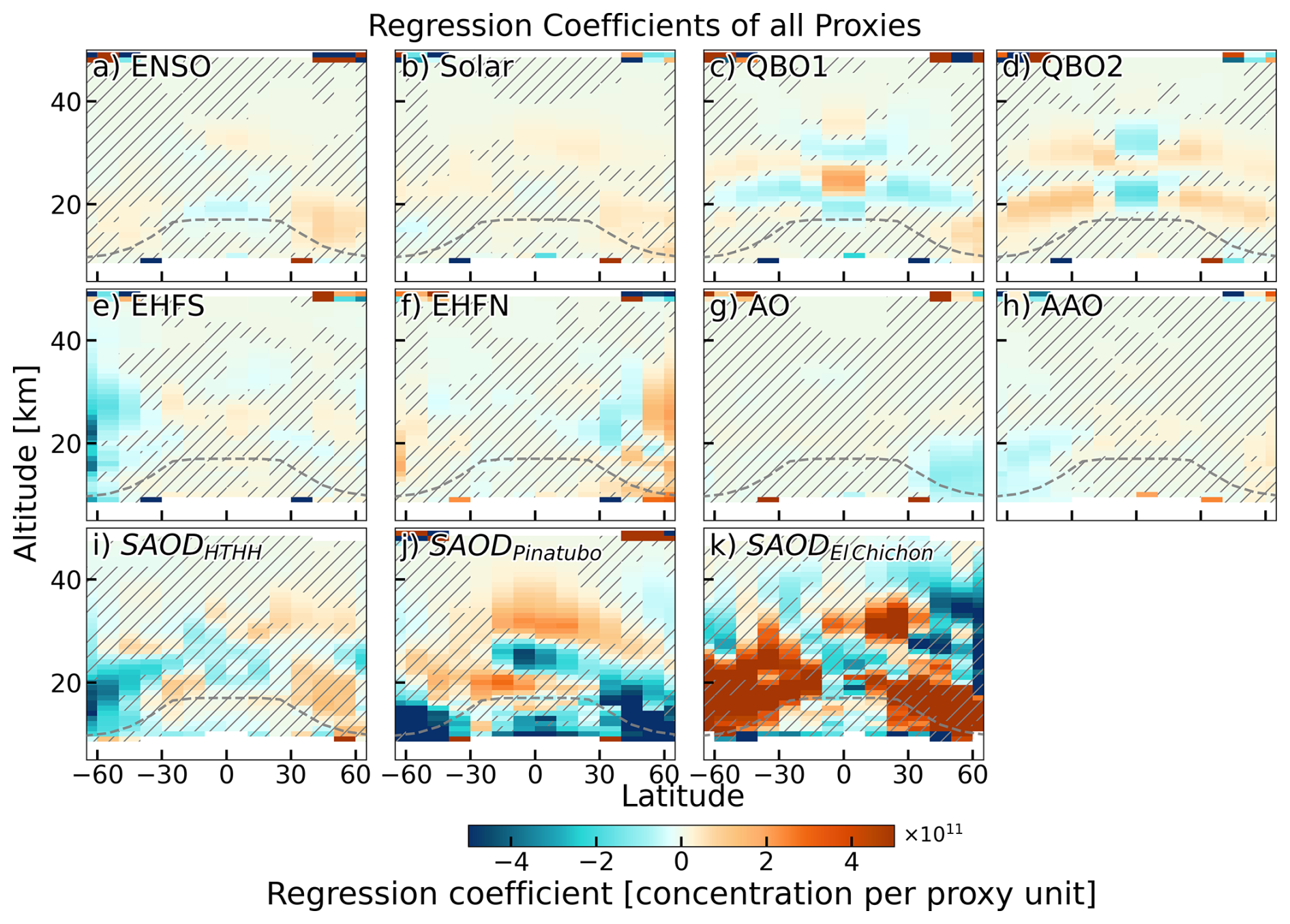
Figure 6 Regression coefficients for (a) ENSO, (b) Solar, (c) QBO1, (d) QBO2, (e) EHFS, (f) EHFN, (g) AO, (h) AAO, (i) SAOD (HTHH), (j) SAOD (Pinatubo) and (k) SAOD (El Chichon) from an MLR fit applied to SWOOSH. Note that EHFS proxy has the opposite sign of EHFN; therefore, lower (more negative) EHFS leads to increases in ozone. All proxies were normalized to −0.5 to 0.5 apart from the SAOD proxies (i), (j) and (k), which were normalized to 0 to 1. Dashed lines are the climatological thermal tropopause derived from ERA5.

Snow et al. (2014)Hersbach et al. (2020)Kovilakam et al. (2020)Kovilakam et al. (2020)Kovilakam et al. (2020)NOAA (2025c)NOAA (2025b)NOAA (2025a)Hersbach et al. (2020)

Table 2 .Overview of proxies used in this study. Data are collected at https://www.iup.uni-bremen.de/OREGANO/proxy/ (last access: 3 March 2026).

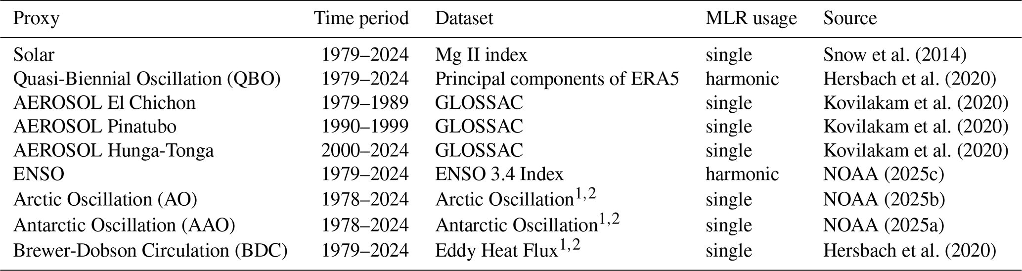
¹ Spring/winter accumulated. ² Ozone-variability weighted.

In this study, the aerosol proxy is separated into three distinct time periods corresponding to the El Chichón period (1979–1989), the Pinatubo period (1990–1999), and the post-2000 period (2000–2024), which includes a series of medium volcanic eruptions as well as the HTHH eruption (Sofieva et al., 2024). Volcanic eruptions have different impacts on stratospheric circulation, chemistry, and ozone distribution, depending on magnitude, season, and latitude of the event (Stolarski et al., 2006; Chehade et al., 2014; Weber et al., 2018, 2022). This variable response is illustrated in panels i–k of Fig. 6. The Australian wildfire (end of 2019) and HTHH had a stronger initial impact in the SH than in the NH because the volcanic aerosols (and stratospheric water vapour) were transported mostly into the SH resulting in an ozone loss (band of negative values in panel i). The Pinatubo eruption had a stronger impact in the NH (boreal winter) as illustrated by the band of negative coefficients from the tropics to the polar region (panel j, Aquila et al., 2014). The dynamic response to the El Chichón eruption showed the opposite effect. Due to changes in the SH circulation the dynamical ozone increase exceeded the chemical ozone loss caused by the eruption (see panel k, Zerefos et al., 1994; Angell, 1997). However, nearly all El Chichon coefficients are not statistically significant at 95 % confidence level. Because of very different ozone responses the major eruptions of El Chichón and Mount Pinatubo are treated separately in the regression. With the 2022 eruption of Hunga Tonga–Hunga Ha’apai (HTHH), a third strong volcanic event occurred that clearly affected stratospheric dynamics and composition (Zhu et al., 2025). Multiple SAOD proxies are also used because the eruptions of El Chichón and, in particular, Pinatubo produce substantially stronger and longer-lasting perturbations to ozone than later eruptions and thus dominate the regression if a single aerosol proxy is used. Treating these periods separately allows the regression model to better represent the variable volcanic forcing (Stolarski et al., 2006; Chehade et al., 2014).

The aerosol data are taken from the GLOSSAC climatologies (Kovilakam et al., 2020). The solar proxy is represented by the Mg II index time series (Snow et al., 2014). The Quasi-Biennial Oscillation (QBO) is described by the first two principal components from a PCA analysis of mean ERA5 stratospheric winds between −6 and 6° latitudes from 70 to 10 hPa. ENSO is described by the ENSO 3,4 index time series. In the past, the El Niño–Southern Oscillation (ENSO) index (MEI V2, Wolter and Timlin, 2011) was used, but we suspect a possible drift starting in the early 2020s, making the index during the recent strong El Niño in 2023/24 too weak (Fig. A1). Additional seasonal components are added to the solar, QBO, and ENSO proxies as mentioned above.

5 Results

We applied the setup (Eq. 2) described in Sect. 4 to the six total ozone datasets and the six profile ozone datasets. Input to the MLR is the ozone timeseries of the datasets. While we mostly show trends from 2000 to 2024, the MLR is always applied to the longer period from 1979 (total ozone) and 1985 (ozone profiles) to 2024 with two inflection points starting in January 1996 and January 2000, with a gap period in between. In general, time series that we use for trend computation are filtered to ensure sufficient data coverage. We exclude time series with less than 50 % valid observations for each sub-period defined by the inflection points. Additionally, we look for sufficient spread of data over each sub-period. For this, we want the first and last value of each period to span at least 50 % of the entire time period, otherwise that period will be excluded from the analysis. This procedure effectively removes time series with insufficient data coverage, while also providing the highest amount of usable data for the trend analysis. The impact of these filters is mostly evident in the tropics below the tropopause and in high latitudes (above 60°) for the profile data and is small for total ozone column data.

5.1 Total Ozone Trends

We first evaluate the total ozone datasets (Table 1) for trends after 2000. The trends as a function of latitude (here in 5° steps), shown in Fig. 7, are mostly positive for all latitudes from 2000 to 2024. The blue lines show the results from our full setup, i.e., with dynamical proxies and three AOD, and the orange lines show the results for the so-called LOTUS setup, i.e., no dynamical proxies and single AOD. Most of the total ozone datasets agree very well. In the NH, total ozone recovers by +1 to +1.5 DU per decade (+0.25 % per decade to +0.5 % per decade). In the SH, the trends polewards of 40° increase on average to +3 to +4 DU per decade (+1.3 % per decade to +1.5 % per decade) and become significant when using the full proxy setup. With the LOTUS settings, SH trends are lower remaining at about +1.5 DU per decade and insignificant above 45° S (see also Fig. A2 for the trends in % per decade). The difference between the two proxy setups is the strongest in the SH above 35° while good agreement is seen elsewhere. The hemispheric asymmetry in the ozone trends with the full setup is in line with observations of the hydrogen chloride (HCl) asymmetry. In the SH, HCl has declined faster due to a faster circulation, fostering in turn a faster increase in ozone compared to the NH (Chrysanthou et al., 2025; Dubé et al., 2025). Results shown in Fig. 7 are very similar to those from Weber et al. (2022), who used a very similar proxy setup.

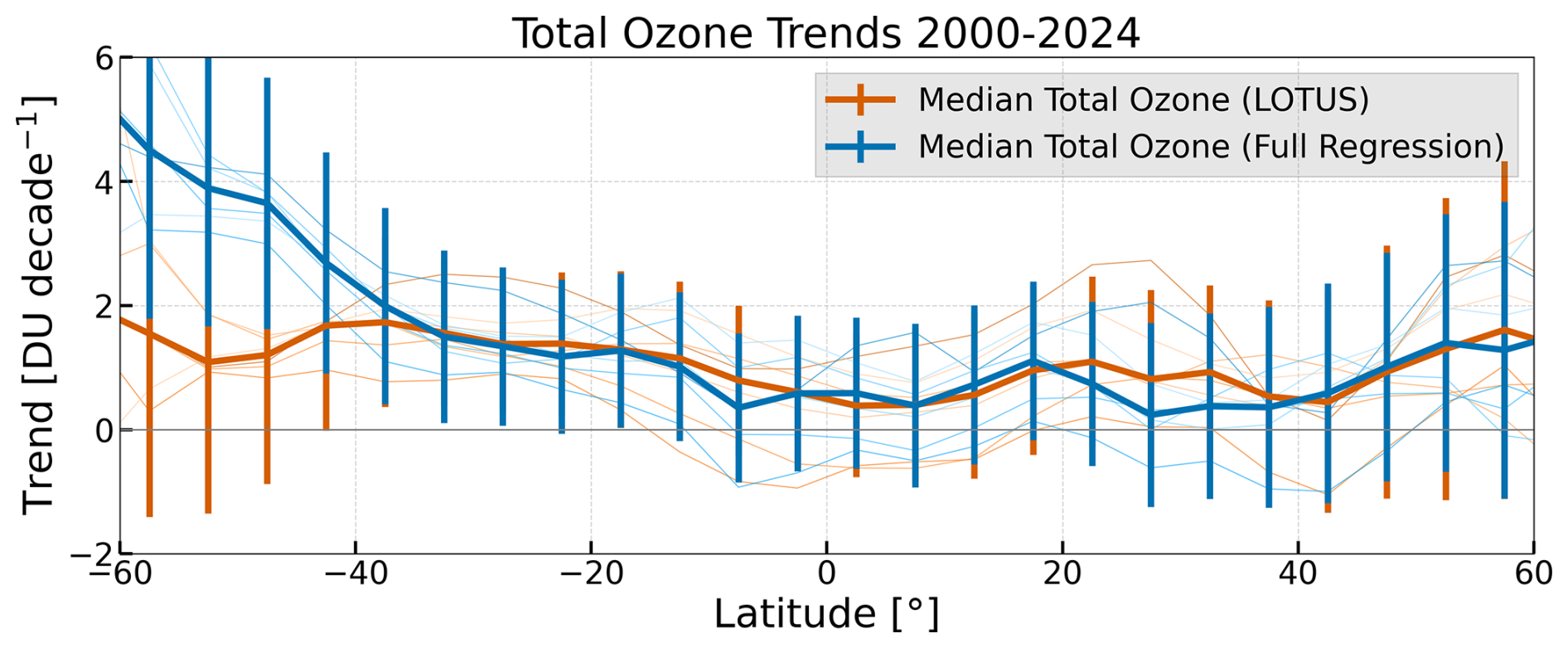
Figure 7 Total ozone trends in DU/decade from 2000 to 2024 for the six total ozone datasets WOUDC, SBUV NASA (MOD), SBUV NOAA (COH), GSG, GTO-ECV, and MSR2 (thin lines) and the median and its 2σ uncertainty (thick line and error bars). Shown in blue are the MLR results with additional dynamical and SAOD proxies and in orange the LOTUS model setup.

To assess differences between the LOTUS model and the full regression model as well as the impact from using the third HTHH SAOD proxy, we look at selected modelled and observed total ozone timeseries. The MLR was applied to the September 60–90° S (ozone hole season) and the 35–60° S annual mean of the six datasets, the results are shown in Fig. 8. A slightly different MLR setup is used here for a more direct comparison to previous analysis by Weber et al. (2022): no gap terms, and in the polar region the pre-ODS period ends in 1999 and post-ODS peak period starts in 2000 (in the extrapolar region 1995 and 1996, respectively) (Newman et al., 2009; Weber et al., 2022). These results can be directly compared to results from Weber et al. (2022). For the southern mid-latitudes, Weber et al. (2022) report an annual trend of 0.7 % per decade for the period 1996–2020 applied to the median timeseries from five total ozone datasets. Extending the analysis to 2024, we obtain trends of 0.6 % per decade (panel c) and 0.4 % per decade with the LOTUS model (panel a). The inclusion of additional dynamical proxies improves the representation of short-term variability, particularly for the local ozone minima in 2020–2022.

A higher difference between the MLR setups can be seen in the southern polar region, where ozone variability and chemical ozone depletion are strongly influenced by the dynamical processes. For September mean ozone between 60 and 90° S, Weber et al. (2022) report a trend of 12.0 % per decade for 2000–2020. In contrast, we derive trends of 3.0 % per decade (LOTUS, panel b) and 8.2 % per decade (full regression), panel (d). Despite the low SH polar ozone in the early 2020s, the full regression trend, interpreted as the smooth ozone recovery related to ODS changes, remains stable within uncertainties after adding four additional years. The impact of dynamical proxies is most pronounced in the polar region (panel d). It is imperative to note, that the LOTUS setup (panel b) was developed for extra-polar latitudes and thus is not suited for polar regions, which is why it only serves as an illustration here.

To demonstrate the impact of the third SAOD (“HTHH”) proxy, we look at the September trends in the SH polar region using different SAOD setups (panel d to f). Polar ozone recovery was first identified in the early phase of the ozone hole season (September) (e.g. Solomon et al., 2016; Weber et al., 2018; Stone et al., 2018). The first setup (panel e) uses a single AOD proxy for the complete time period like in the LOTUS setup, the second (panel f) uses two SAOD proxies, one until 1989 (“El Chichon”) and the other from 1990 to 2024 (“Pinatubo”) (Chehade et al., 2014; Weber et al., 2022), and the last (panel d) uses three SAOD proxies by adding the period 2000–2024 (“HTHH”) and limiting the second SAOD to 1990–1999. The difference between the first (e) and the second (f) setup is small, with trends after 2000 being around +3.5 % per decade in both cases. The addition of the third (d) SAOD (“HTHH”) more than doubles the post-2000 trend to 8.2 % per decade, making it very similar to +12.0 % per decade until 2020 from Weber et al. (2022). These results show the strong sensitivity of the regression and the influence of the dynamical proxies in the southern polar region. Volcanic eruptions lead to perturbations in ozone that usually last for a few years (Wang et al., 2023; Fleming et al., 2024). In the early 2020s, a series of high-stratospheric aerosol events (Australian wildfires in 2019/2020, the 2021 Le Soufrière, and 2022 HTHH volcanic eruption) was responsible for the above-average size ozone holes between 2020 and 2023 (Yook et al., 2022; Fleming et al., 2024). The HTHH-SAOD proxy allows a better separation of these perturbations from the slow (background) decreases in ODS responsible for ozone recovery. The effect from the SAOD-HTHH proxy is however negligible for extrapolar total ozone, but the MLR pattern of the regression coefficient of the HTHH proxy shown in panel (i) of Fig. 6 seems physically reasonable. In summary, the use of the dynamical and SAOD-HTHH proxies in the MLR as well as the comparisons with the earlier results for the period ending in 2020 prove that ozone recovery is ongoing despite the ozone perturbations in the early 2020s in response to the series of volcanic and wildfire events.

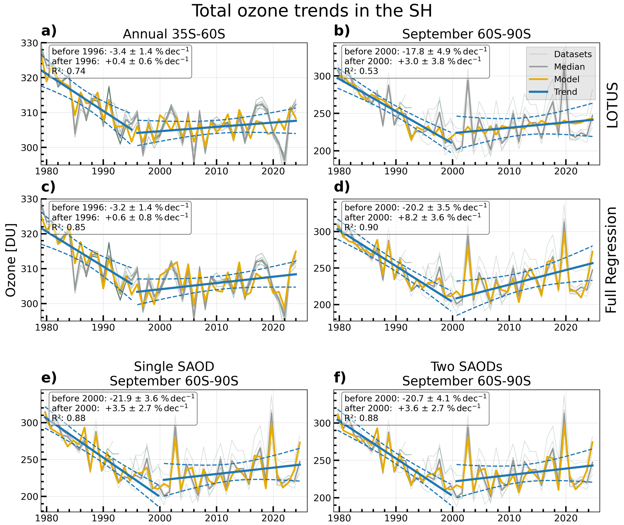
Figure 8 35–60° S annual mean (a, c) and 60–90° S September (b, d, e, f) MLR results using the LOTUS setup (top row) and the full regression model (second row) applied to the total ozone median from six merged datasets. Different SAOD setups are shown for the September SH polar region: (e) single AOD proxy from 1979 to 2024, (f) two AOD proxies: from 1979 to 1989 and from 1990 to 2024 and (d) three AOD proxies: from 1979 to 1989 (El Chichon period), from 1990 to 1999 (Pinatubo period), and from 2000 to 2024 (HTHH and smaller eruption period). Thick grey line: median of observations; yellow line: MLR regression; thin grey lines: individual merged datasets; solid blue lines: trend lines before and after 2000; dashed blue lines: 2σ uncertainty of the trend lines.

5.2 Ozone profile trends 2000–2024

Figure 9 shows ozone profile trends as a function of latitude and altitude for the period 2000 to 2024 using the same setup as for total ozone (Eq. 2). Generally, there is good agreement between the datasets. Above 30 km the trends are below +0.1 DU km⁻¹ per decade as ozone concentration decreases with altitude. Below 30 km, the ozone trends increase up to 0.5 DU km⁻¹ per decade and contribute substantially to the total ozone trends. Negative trends with high uncertainties are mostly visible below 20 km, close to the tropopause. In the UTLS region, uncertainties in limb ozone measurements are higher and likely responsible for higher trend uncertainties (Rahpoe et al., 2015; Hubert et al., 2016).

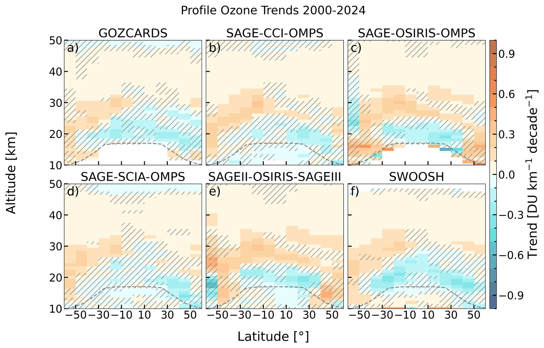
Figure 9 Profile ozone trends in DU km⁻¹ per decade from 2000 to 2024 from the six merged ozone datasets as a function of latitude and altitude: (a) GOZCARDS , (b) SAGE-CCI-OMPS, (c) SAGE-OSIRIS-OMPS, (d) SAGE-SCIA-OMPS, (e) SAGEII-OSIRIS-SAGEIII, and (f) SWOOSH. Hatched areas indicate regions of no significance (2σ). Dashed lines are the climatological thermal tropopause derived from ERA5.

Ozone profile trends in units of % per decade are shown in Fig. A3 of the Supplement. The trends observed in our study (Fig. A3) mostly agree with the results from Sofieva et al. (2026), but there are some differences. The positive trends in the upper stratosphere are consistent between both studies (about +1 % per decade to +3 % per decade). A belt of negative trends just above the tropopause appears to be more persistent from 60° S to 60° N in Fig. 1 of Sofieva et al. (2026) and negative trends in the UTLS appear to be less negative in our case. This is also seen when comparing to a MLR setup without the AO, AAO, EHFS, and EHFN and with a single SAOD proxy (LOTUS setup), as shown in Figs. A4 and A5.

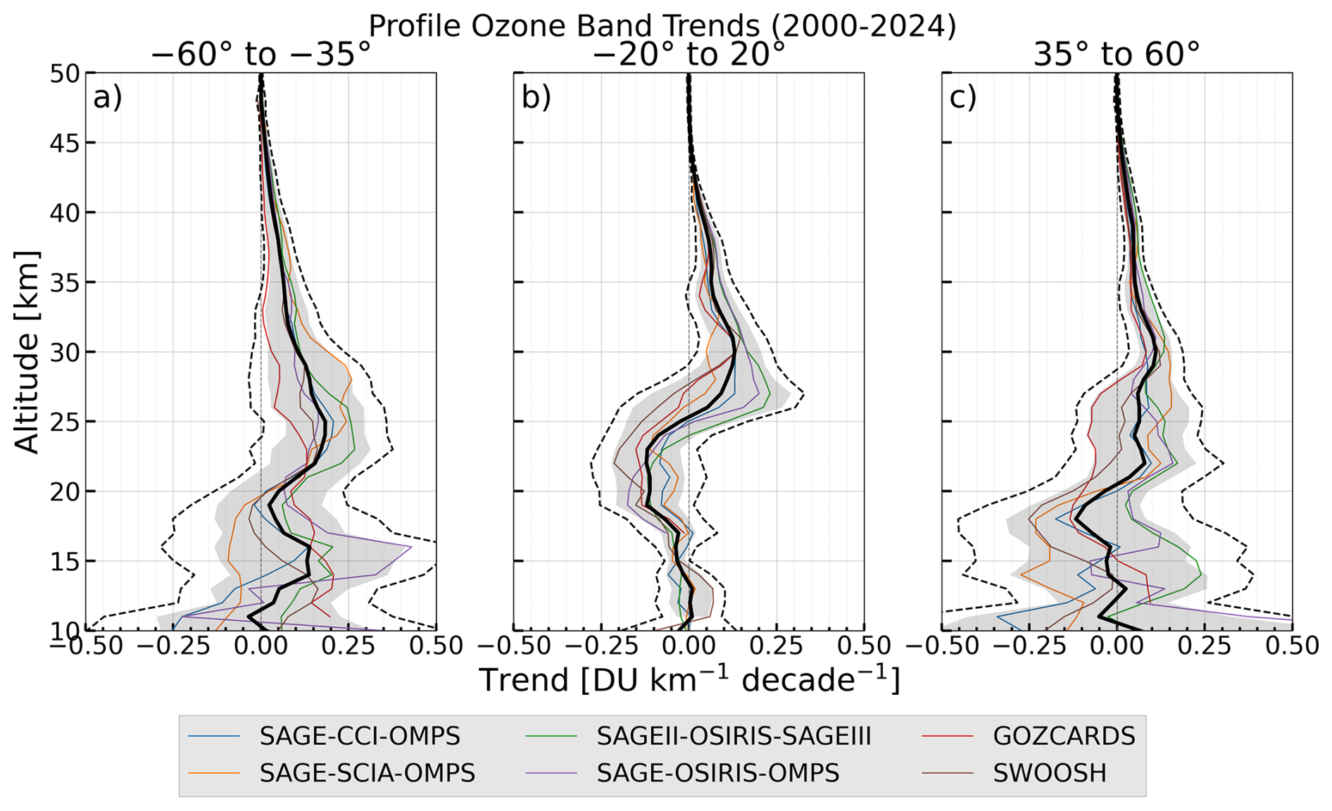
Figure 10 Ozone trends from 2000 to 2024 in three latitude bands ((a) 35–60° S, (b) 20° S–20° N, (c) 35–60° N) in DU km⁻¹ per decade for the six merged ozone profile datasets: GOZCARDS, SAGE-CCI-OMPS, SAGE-OSIRIS-OMPS, SAGEII-OSIRIS-SAGEIII, SAGE-SCIA-OMPS, and SWOOSH. Shaded area indicates the 2σ uncertainties of the mean trends (black line), calculated using the LOTUS uncertainty estimate described in Eq. (7) and the dashed line indicates the J-Distribution uncertainty described by Eq. (9).

In the lower to middle stratosphere (above 20 km altitude), a hemispheric asymmetry in trends is noticeable, with higher trends in the SH, a pattern similar to what is observed for total ozone in Fig. 7. This asymmetry is also seen when looking at trends in three broad latitude bands. Figure 10 shows the ozone profile trends for the zonal bands, 35–60° S (SH), 20° S–20° N (tropics) and 35–60° N (NH). Below 30 km altitude, trends are smaller in the NH compared to the SH. There is overall good agreement in the broad band trends between the datasets. All datasets agree on a positive trend above 30 km in all three latitude bands, maximizing at between 1 % per decade to 3 % per decade near 43 km altitude (Fig. A7). The SH displays larger variations in trends between datasets in this altitude region. The tropics show negative trends below 25 km for all datasets. In the extratropics trends below 20 km can be both positive and negative depending on the dataset. Below about 20 km altitude, the uncertainty in the mean trend increases.

The broad zonal band trends (Fig. 10) show the band trends, similar to Sofieva et al. (2026). The corresponding representation in % per decade (Fig. A7) can be compared with those shown in Fig. 4 of Sofieva et al. (2026), which were derived using the LOTUS setup and cover the same time period up to 2024. Upper stratospheric trends agree well between both studies. Differences are visible in the lower stratosphere. As mentioned before, the lowermost stratospheric mean trends are negative in the extratropics in Sofieva et al. (2026), while in our study they are positive in the SH and on average closer to zero in the NH (see also Figs. A8 and A9). Mirallie et al. (2026) show consistently positive trends in the upper stratosphere, while finding mixed and negative trends in the middle and lower stratosphere from ground-based measurements

The larger variations in SH trend profiles for altitudes above 25 km, seen in panel a) of Fig. 10 (see also Figs. A7–A9) is due to the smaller positive trends seen in GOZCARDS compared to all other merged datasets. Applying the MLR to deseasonalized ozone data (rather than absolute values), GOZCARDS trends in the SH are getting closer to the trends of the other data, as shown in Sofieva et al. (2026).

The differences between the LOTUS uncertainty estimate (shaded area) and the joint-distribution approach (dashed lines) are largest at lower altitudes, where the trends from the individual datasets show higher differences. This is particularly evident in the mid-latitudes around 17 km, most likely driven by both higher trend differences and differences in the underlying dataset uncertainties. While the LOTUS uncertainty estimate generally envelops the individual trends, with some exceptions for datasets exhibiting pronounced trends at specific altitudes, the joint-distribution approach spans a wider range, as it characterizes the total ensemble variance.

5.3 Comparison of total and stratospheric ozone column trends

We calculate the stratospheric columns by integrating the ozone profiles upward from the ERA5 climatological thermal (lapse rate) tropopause. Another method to calculate the stratospheric ozone column trends is to integrate the ozone layer trends shown for example in Fig. 9. A comparison between the two methods (Fig. A6) show that the trends from both methods are generally very similar, however, the uncertainty of the vertically integrated layer trends are smaller than for the trend derived from stratospheric column trends. The tropopause height is determined at the center of each latitude band using interpolation. The MLR is then applied to the stratospheric columns. The difference between total column and stratospheric column trends can then be attributed to the tropospheric contribution to total ozone trends.

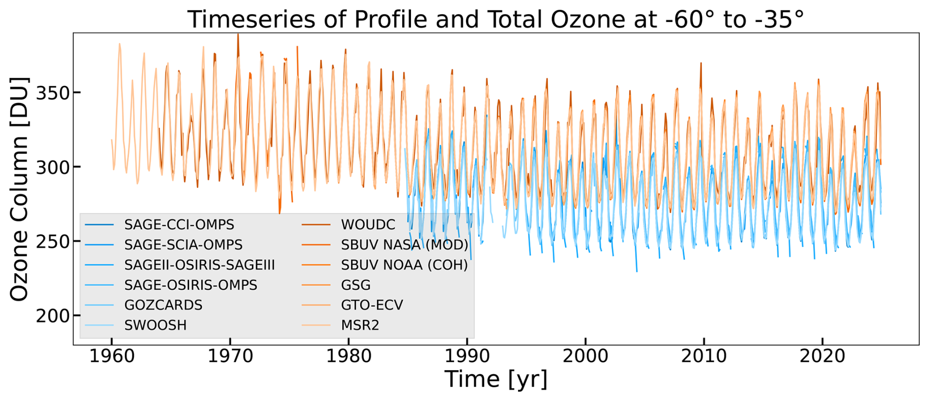
Figure 11 Observed zonal debiased mean stratospheric (blue) and total (orange) ozone columns in the 35 to 60° S latitude band.

Figure 11 shows as an example the ozone timeseries in the broad zonal band 35–60° S for stratospheric ozone and total ozone columns of all datasets. The stratospheric ozone column was bias-corrected by subtracting the mean during the 1998–2008 period from each dataset (anomaly) and adding back the multi-instrument mean to obtain bias-corrected absolute ozone values for each dataset. The difference between the total and stratospheric columns of about 20 to 30 DU yields the zonal mean tropospheric column. There is a gap in the stratospheric column timeseries after the eruption of the Pinatubo volcano in 1992, because of filtering of columns that did not reach the tropopause. This is mainly due to retrieval artifacts in the presence of layers of high aerosol extinction obstructing the limb view in the lowermost stratosphere. The total ozone datasets seem less affected. Due to the weaker eruption of HTHH in 2022 in terms of stratospheric aerosol load, this impact on stratospheric column calculation is also reduced except for SAGE-SCIA-OMPS. For this dataset, observations from February 2022 to May 2023 were excluded.

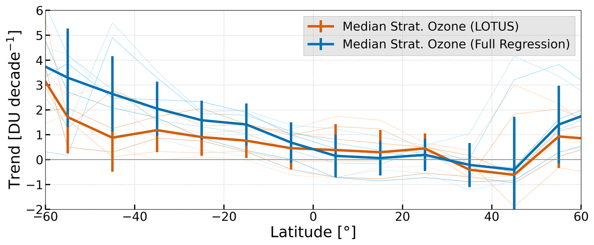
Figure 12 Stratospheric ozone trends in DU per decade from 2000 to 2024 for the six profile ozone datasets GOZCARDS, SAGE-CCI-OMPS, SAGE-OSIRIS-OMPS, SAGE-SCIA-OMPS, SAGEII-OSIRIS-SAGEIII and SWOOSH (thin lines) and the mean and its 2σ uncertainty (thick line and error bars). Shown in blue are the MLR results with additional dynamical and SAOD proxies and in orange the LOTUS model setup.

Figure 12 shows the results of the stratospheric column trends as a function of latitude which can be compared to the total ozone trends (Fig.  7). The tropics and the NH show very similar results with low ozone trends in the tropics (+0.0 to +1 DU per decade) and slightly higher ozone trends above 40° N (up to 2 DU per decade) for both proxy setups. The differences which we saw in the SH total ozone can be seen here as well. Trends using the full setup are larger (up to +3.5 DU per decade) than using the LOTUS setup (+2 DU per decade). Both proxy setups yield similar trends in the SH for stratospheric and total columns, but the stratospheric column trends show a much higher spread between the trends of the different datasets compared to total ozone.

In Fig. 3b of Sofieva et al. (2026) combined latitude-dependent stratospheric column trends are shown and can be compared to our results. Above 40° latitude in each hemisphere stratospheric column trends using the LOTUS setup are slightly higher (around 2 DU per decade) in our analyses compared to Sofieva et al. (2026) (around 1 DU per decade). This difference likely arises from the comparatively strong trends in the OSIRIS dataset, which exert a larger influence on the multi-dataset mean in our six-dataset ensemble than in the eight-dataset mean used by Sofieva et al. (2026). Below 40° the stratospheric column trends agree.

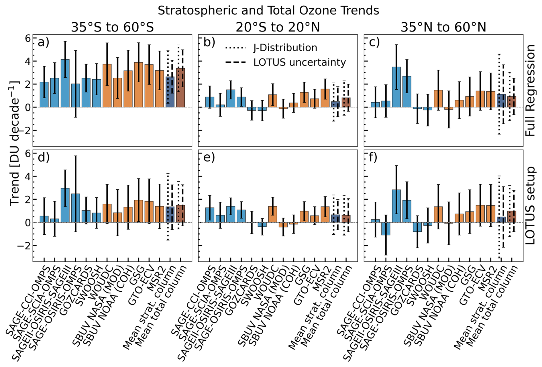
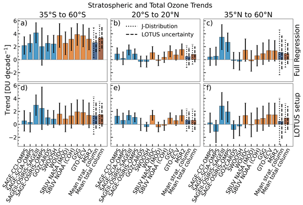
Figure 13 Broad band zonal mean ozone column trends from 2000 to 2024. Shown are total column trends (orange) and stratospheric column trends (blue) for each merged datasets. Upper row panels show the results using the full MLR regression and lower row panels show the regression with the LOTUS setup. Zonal bands are (a, d) 35–60° S, (b, e) 20° S–20° N, (c, f) 35–60° N. Black error bars indicate the 2σ trend uncertainties. The last two bars in each panel show the mean stratospheric and total column ozone trends with two error bars each calculated using the LOTUS (dashed) and the J-distribution (dotted), respectively.

Figure 13 shows trends for all datasets from 2000 to 2024 in the three broad zonal bands. The bars represent the stratospheric ozone column (light blue) and total ozone column trends (orange) of the individual merged datasets. The last two bars show the mean stratospheric ozone column (dark blue) and the mean total ozone column (brown).

The agreement between stratospheric and total column trends is remarkably close across all latitude bands (panels a to c). This suggests that the contribution of tropospheric ozone to the total column trends is small and well below the trend uncertainties. Significant positive stratospheric and total column trends are visible in the SH (about +2 to +4 DU per decade). On average, smaller trends (about +1 DU per decade) are seen in the tropics and the NH in agreement with Figs. 7 and 12. The two merged ozone profile datasets that include OSIRIS (SAGEII-OSIRIS-OMPS and SAGEII-OSIRIS-SAGEIII) show larger trends in comparison to the other ozone profile datasets in the extratropics. Both profile datasets that contain Aura/MLS at the end of their data record (GOZCARDS and SWOOSH) show, not unexpectedly, nearly the same trends.

The bottom row of Fig. 13 (panels d to f) shows our MLR results using the LOTUS setup. The mean profile trends are about +1 DU per decade in the SH and are smaller than with the full proxy setup except for the two merged datasets including OSIRIS and are mostly positive in the other two bands, similar to the full proxy trends.

The ground-based dataset WOUDC total ozone trends are consistent with the trends of the satellite-based datasets. Although WOUDC total ozone values are occasionally slightly higher than the satellite-based datasets (Fig. 11). The LOTUS and the J-distribution uncertainty estimates are showing similar results for total ozone, while the J-distribution uncertainty is mostly larger than the LOTUS uncertainty for the mean stratospheric column trends (Steinbrecht et al., 2017; Petropavlovskikh et al., 2019).

6 Discussion

The ozone profile datasets generally start at an altitude of 10 km (Table 1) which can be an issue when the tropopause is lower than 10 km, particularly at higher latitudes. For the stratospheric column calculations, data were screened out if the three lowest 1 km layers above the tropopause had missing data. In combination with the larger uncertainties of limb measurements below 20 km, this selection criterion causes larger spreads in the profile and stratospheric column trends.

The conversion of the merged ozone profile datasets to a common vertical grid and ozone unit was done for GOZCARDS and SWOOSH and this leads to additional trend uncertainties as that conversion had to be applied to monthly mean data rather than single ozone profiles before merging. In most cases it was found that the difference between both conversions (monthly mean versus single profiles) is statistically not significant, but for certain altitude regions and months it is non-negligible (Fig. 3). As these differences were mostly negative, the trends reported for GOZCARDS and SWOOSH may be slightly underestimated. To have a comparison of ozone trends on the same grid and with the same units as the other datasets, a conversion of pressure to geometric altitude and volume mixing ratio to number density was needed. The same method that was used for the other datasets to calculate the stratospheric column was then used for GOZCARDS and SWOOSH as well.

An additional uncertainty arises from temperature trends in the stratosphere. Conversion between pressure and altitude coordinates follows from the hydrostatic equation and therefore depends on atmospheric temperature. Long-term temperature changes induce vertical shifts of geometric altitude relative to pressure levels, which can alter vertical ozone gradients and modify the trends. As discussed by McLinden and Fioletov (2011) and in the LOTUS assessment (Petropavlovskikh et al., 2019), ozone trends derived on pressure levels (e.g., VMR) can differ from trends derived on altitude levels (e.g., number density) when substantial temperature trends are present. Before the late 1990s, pronounced upper-stratospheric cooling contributed to such discrepancies. For the post-2000 period analyzed in this paper, upper-stratospheric temperature trends are considerably weaker (e.g. Thompson et al., 2011). In the upper troposphere–lower stratosphere (UTLS), recent satellite-based analyses reveal vertically structured temperature trends and changes in lapse-rate tropopause height during the 21st century (Ladstädter et al., 2023, 2025). Such structural changes may slightly affect local ozone gradients. However, given the comparatively small magnitude of recent temperature trends, temperature-driven effects are expected to remain a smaller contribution to the ozone trend estimates presented here.

A major point of discussion in this study concerns the choice of the proxy setup used in the MLR model. In contrast to the standard proxy configurations used in recent ozone trend studies (e.g., Godin-Beekmann et al., 2022; Sofieva et al., 2026), we extended the set of independent variables to include the AO, AAO, and the BDC. We also separated the SAOD proxy into three distinct periods that included the large eruptions of El Chichon (1979–1999), Pinatubo (1990–1999), and Hunga-Tonga (2000–2024). Depending on the location and season of the eruptions, the dynamical response (circulation) from these eruptions may differ (e.g. Chehade et al., 2014). This expanded proxy configuration was chosen to better capture the dynamical and chemical variability observed in the past two decades (Weber et al., 2022). As shown in Fig. 8, the full regression is generalised in such a way that it covers the variability in and outside the polar region. The use of three SAOD proxies/periods brings total ozone trends at SH middle latitudes and the south polar region in better agreement with results from Weber et al. (2022), which clearly indicate that the path of recovery remains within uncertainties unchanged from the earlier study, by using additional four years and despite lower ozone in the early 2020s. The HTHH-SAOD proxy accounts to some extent also for the effect from the enhanced water vapor following the underwater eruption of HTHH (Vömel et al., 2022; Millán et al., 2022). Changes in transport/circulation had a larger influence on ozone than altered chemistry due to enhanced chlorine activation following the eruption (Oesterstroem and Santee, 2025). The additional HTHH-SAOD proxy was introduced to properly model the negative ozone perturbations during a short period of about three years (2020–2022) with elevated stratospheric aerosols at middle to high latitudes in the SH. Without this proxy, the retrieved trends until 2024 are significantly lower than the reported trends until 2020 (WMO, 2022; Weber et al., 2022). From the continuous and nearly linear decline in ODS since 2000, ozone recovery trends (due to ODS changes only) are expected to remain unchanged within uncertainty. With the addition of the third SAOD proxy and the dynamical proxies, this is the case.

In total, the MLR model (Table 2) includes 23 proxy variables together with the intercept and trend terms. While the number of fit parameters is higher than in most previous studies (Godin-Beekmann et al., 2022; Sofieva et al., 2026), the large temporal extent of the dataset, covering 24 years at a monthly resolution (288 data points per time series), provides sufficient degrees of freedom and does not necessarily imply overfitting, even in the presence of autocorrelation in the timeseries. We find that the inclusion of the AO, AAO, and BDC proxies improves the representation of inter-annual and sub-decadal variability, particularly during years with strong polar vortex disturbances. The change from a single AOD proxy to three independent AOD proxies (Fig. 8) also improved the model by better capturing the ozone maxima and minima. While stratospheric and total column trends are very similar without and with the additional dynamical proxies (Figs. 7 and 12), the largest impact from the additional proxies is evident at middle to high latitudes in the SH, where LOTUS total ozone trends (+2 DU per decade) are half the values found in this study (+4 DU per decade). This indicates the impact of dynamics on ozone trends. The stratospheric column shows somewhat smaller differences between the two methods. The reason for this might come from the high variability of the ozone profile trends at high latitudes.

A comparison of our results, using the LOTUS setup (Fig. A7) with recent ground-based studies (Mirallie et al., 2026) shows a general agreement in the vertical structure of the ozone trends. In both studies, the largest positive trends are found in the upper stratosphere, consistent with ongoing ozone recovery. Mirallie et al. (2026) show clear negative trends between 20 and 30 km in the tropics and more mixed results in the northern hemisphere. This mostly mirrors our results although a slightly different proxy setup was used. The most notable difference is a slightly positive trend in the northern hemisphere above 20 km in our results, while Mirallie et al. (2026) show mixed results depending on the station (Figs. 20–23). This might highlight the need to look more closely at longitudinally resolved trends in a future study.

The histogram shown in Fig. 13 provides a very similar picture. Using the joint distribution (Ko et al., 2013) to calculate the uncertainties, the 2σ uncertainties for the mean stratospheric and total column trends are mostly larger than the trends itself, except for the mean total ozone trends in the latitude band 35–60° S using the full proxy setup (panel a). A substantial part of these uncertainties can be attributed to relative drifts between the individual datasets. Globally after 2000, the 1σ spread of the drift estimates between the ozone profile datasets is around 1 % per decade (+1 DU per decade) and increases strongly below 20 km (Fig. 4). For total ozone, the corresponding 1σ spread is smaller, about 0.1 % per decade to 0.3 % per decade, or 0.3 to 1 DU per decade, but still contributes noticeably to the total trend uncertainty (Fig.  5). Within uncertainties, the mean zonal stratospheric column trends do not differ from total ozone and the tropospheric ozone trend contribution (from the difference between both) is therefore not relevant.

Overall, the extended proxy setup provides a more comprehensive and physically consistent description of the processes influencing stratospheric and total ozone variability globally, and in particular, in the polar region (see Fig. 8).

As it was briefly commented in Sect. 5, the ozone profiles and, with that, the stratospheric ozone trends have mostly large uncertainties and are also not as uniform in their trends as for total ozone. Such increased uncertainties in vertically resolved ozone, particularly close to the UTLS region, have also been reported recently by Davis et al. (2026), where discrepancies among observational ozone profile datasets, particularly in the lowermost stratosphere, were found. These uncertainties propagate into the derived stratospheric column ozone and therefore need to be considered when interpreting the computed trends.

7 Conclusions

We analyzed long-term ozone trends from 2000 to 2024 using multiple merged satellite profile and total column datasets. After harmonizing profile data to a common altitude grid, stratospheric column trends were calculated and compared directly with independent total ozone trends. Trends were estimated using a multiple linear regression model that includes an extended set of dynamical proxies to better capture inter-annual variability and recent circulation anomalies. All profile datasets consistently indicate continued ozone recovery in the upper stratosphere, particularly in southern mid-latitudes. In contrast, lower stratospheric trends remain weak and regionally variable, with negative tendencies in parts of the tropics. When integrated to stratospheric columns, the resulting trends closely match those derived from total column datasets across all latitude bands. Within statistical uncertainties, this agreement suggests that total ozone recovery since 2000 is primarily driven by changes in the stratosphere. Tropospheric ozone trends do not produce a detectable large-scale signal in total column trends over this period. The extended regression configuration improves the representation of recent high-variability years and volcanic influences. The main conclusions are positive upper-stratospheric trends and close agreement between total and stratospheric column changes within the combined trend uncertainties. Using the full regression with additional dynamical proxies and three separate SAOD proxies, the later representing different periods of strong stratospheric aersol enhancements, leads to higher extratropical column trends in the SH compared to the NH after 2000, which is in line with indications of a faster ozone recovery in the SH due to a faster decline in the HCl reservoir gas as a result from a faster meridional circulation (Chrysanthou et al., 2025; Dubé et al., 2025). These results provide an updated assessment of ozone recovery through 2024 and reinforce evidence that the Montreal Protocol continues to yield measurable atmospheric benefits.

Appendix A

Froidevaux et al. (2015)Sofieva et al. (2017)Bourassa et al. (2014)Arosio et al. (2019)Bognar et al. (2022)Davis et al. (2016)van der A et al. (2015)Weber et al. (2022)Coldewey-Egbers et al. (2015, 2022)Frith et al. (2014, 2017)Fioletov et al. (2002, 2008)

Table A1 Sources of the ozone datasets that were used in this study.

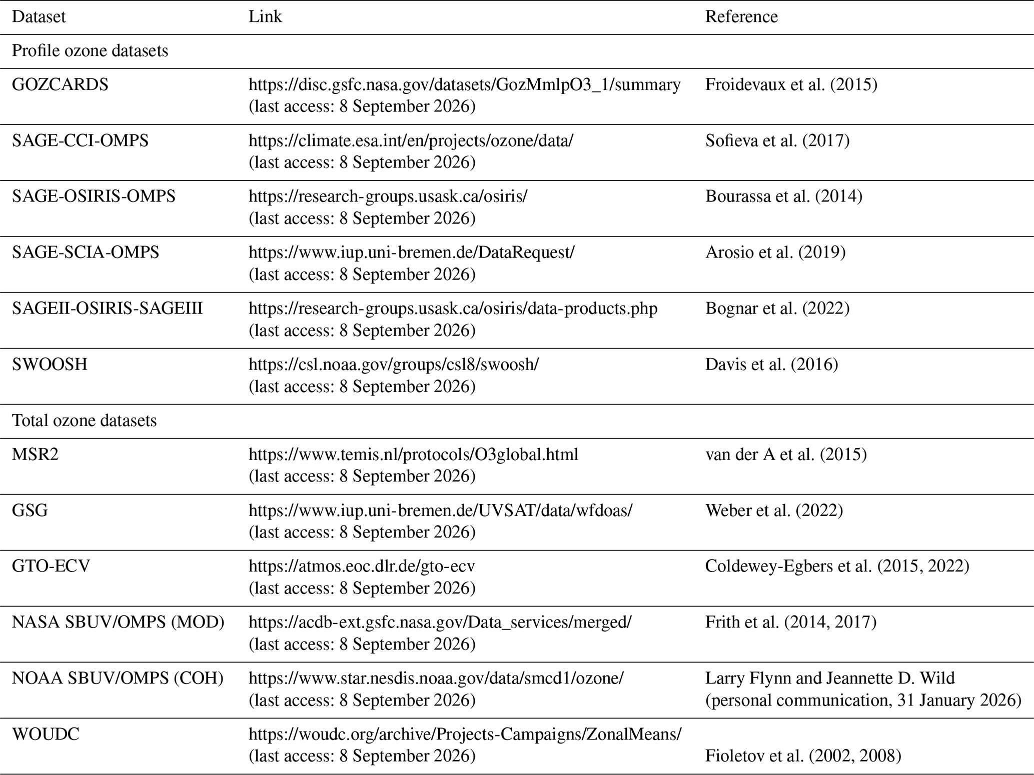
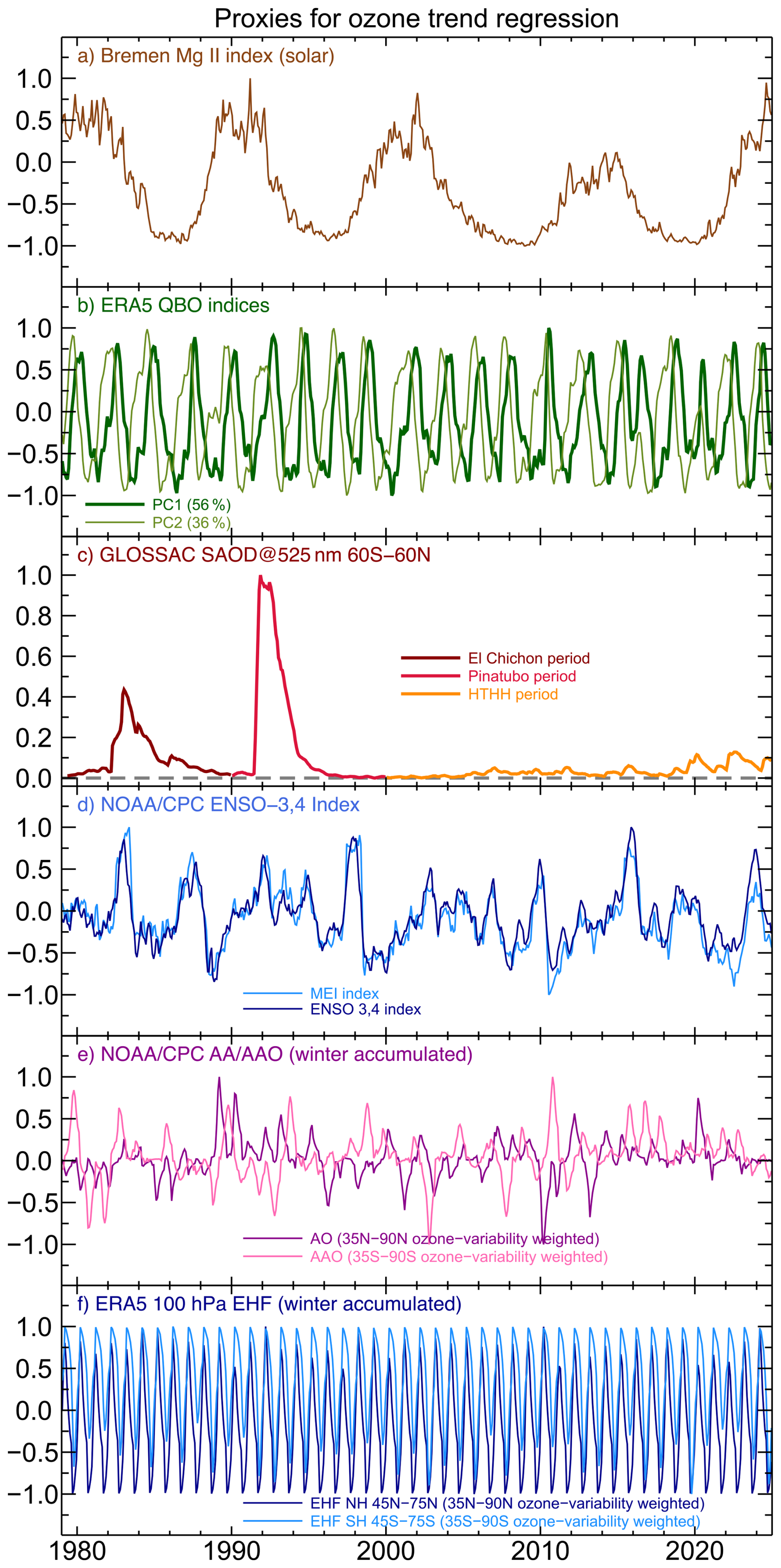
Figure A1 Proxies used in the full regression model. Proxies shown are (a) Solar, (b) QBO1/QBO2, (c) SAOD (with the three periods shown in different colors), (d) ENSO, (e) AO/AAO and (f) EHFN/EHFS. The AO, AAO and EHFn/EHFs are winter/spring accumulated and ozone-variability weighted, as described in Sect. 4.2. Ozone-variability weights are latitude dependent. The SAOD proxies are determined for the latitude bands considered in the MLR.

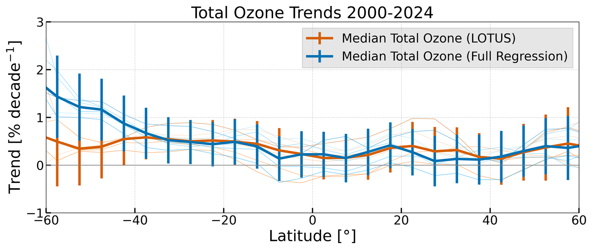
Figure A2 Total ozone trends in % per decade from 2000 to 2024 for the six total ozone datasets WOUDC, SBUV NASA (MOD), SBUV NOAA (COH), GSG, GTO-ECV, and MSR2 (thin lines) and the median and its 2σ uncertainty (thick line and error bars). Shown in blue are the MLR results with additional dynamical and SAOD proxies and in orange the LOTUS model setup. Same as Fig. 7, but with ozone trend units of % per decade.

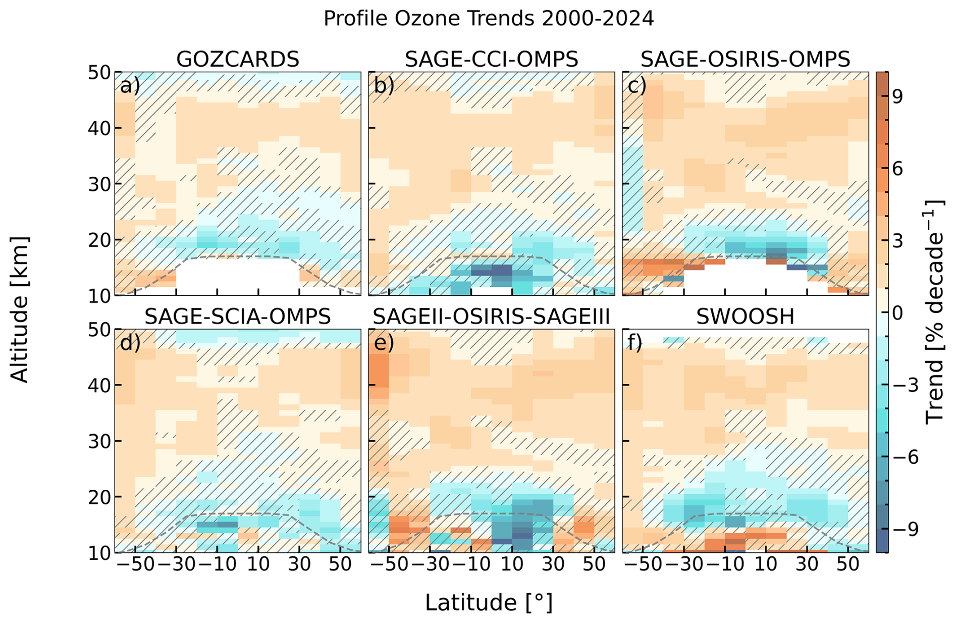
Figure A3 Profile ozone trends in % per decade from 2000 to 2024 for the six profile ozone datasets (a) GOZCARDS, (b) SAGE-CCI-OMPS, (c) SAGE-OSIRIS-OMPS, (d) SAGE-SCIA-OMPS, (e) SAGEII-OSIRIS-SAGEIII, and (f) SWOOSH. Hatches indicate regions of no significance (2σ). Same as Fig. 9, but in units of % per decade.

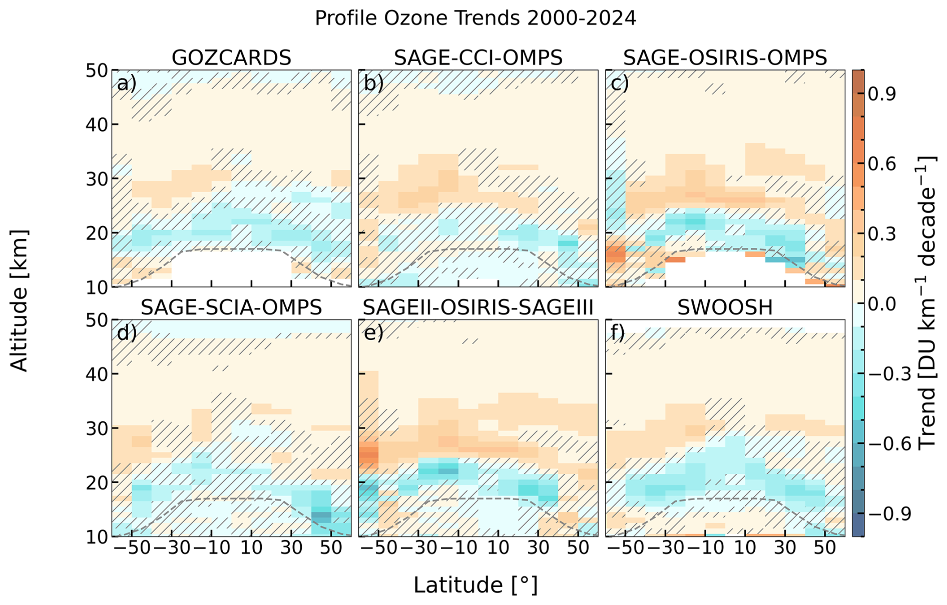
Figure A4 Profile ozone trends (LOTUS model) in DU km⁻¹ per decade from 2000 to 2024 for the six profile ozone datasets (a) GOZCARDS, (b) SAGE-CCI-OMPS, (c) SAGE-OSIRIS-OMPS, (d) SAGE-SCIA-OMPS, (e) SAGEII-OSIRIS-SAGEIII, and (f) SWOOSH. Hatches indicate regions of no significance (2σ). Same as Fig. 9, but using the LOTUS setup in the MLR.

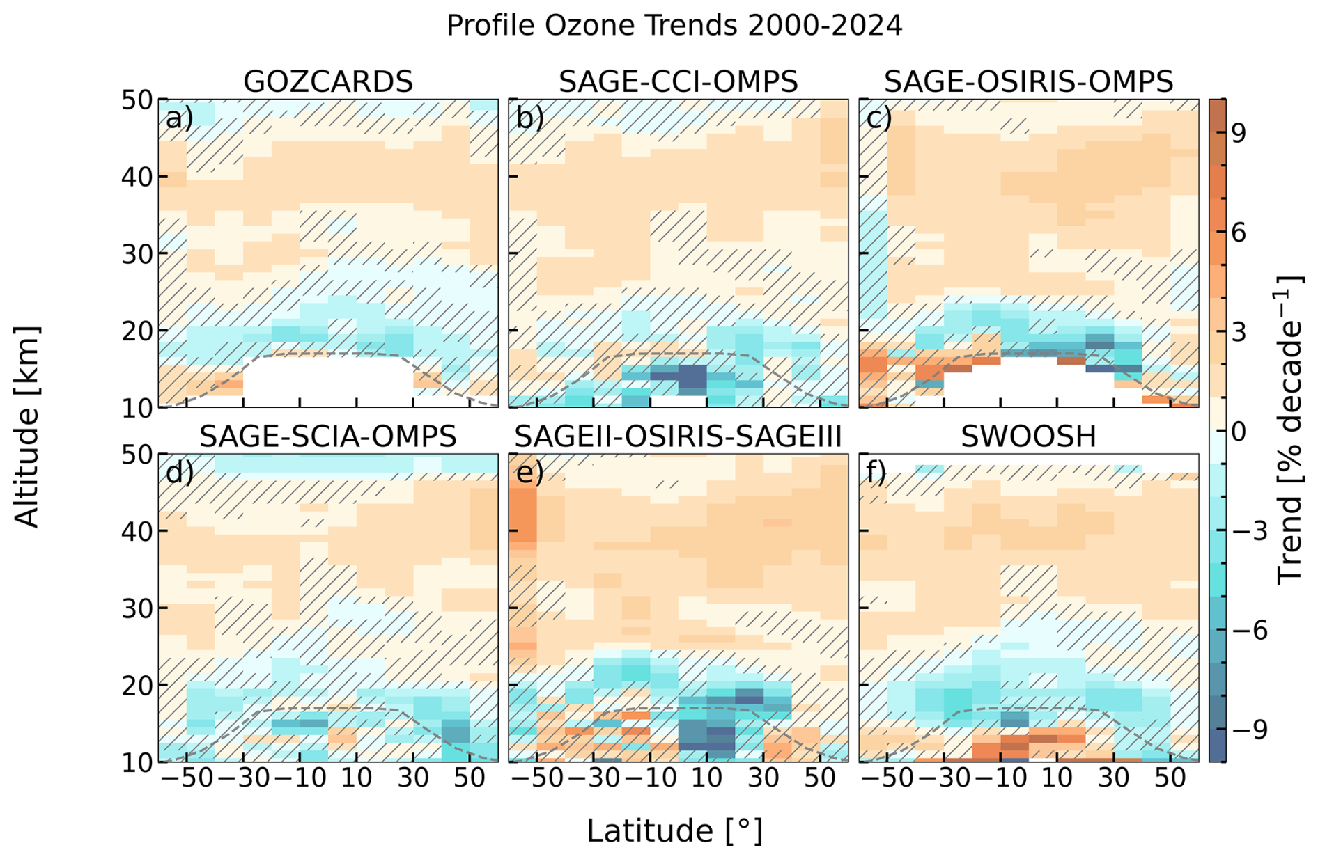
Figure A5 Profile ozone trends in % per decade from 2000 to 2024 using the LOTUS setup for the six profile ozone datasets (a) GOZCARDS, (b) SAGE-CCI-OMPS, (c) SAGE-OSIRIS-OMPS, (d) SAGE-SCIA-OMPS, (e) SAGEII-OSIRIS-SAGEIII, and (f) SWOOSH. Hatches indicate regions of no significance (2σ). Same as Fig. 9, but using the LOTUS setup in the MLR and trend units of % per decade.

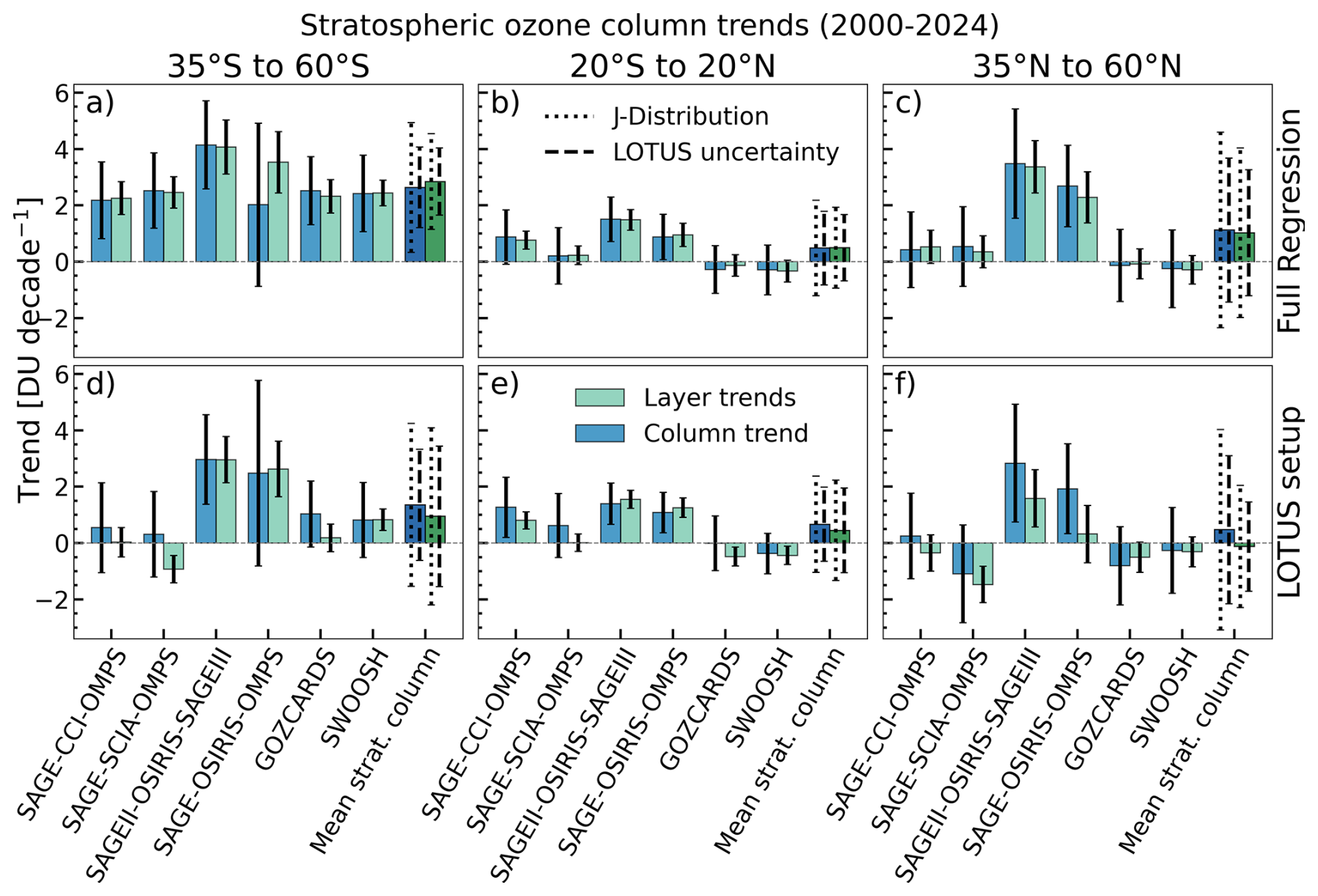
Figure A6 Broad band zonal mean stratospheric ozone column trends from 2000 to 2024. Shown are stratospheric column trends using two approaches: MLR applied to stratospheric columns (dark blue) and stratospheric column trends (light green) determined by integrating ozone layer trends above the thermal tropopause. Upper row panels show the results using the full MLR regression and lower row panels show the regression with the LOTUS setup. Zonal bands are (a, d) 35–60° S, (b, e) 20° S–20° N, (c, f) 35–60° N. Black error bars indicate the 2σ trend uncertainties. The last two bars in each panel show the mean stratospheric column ozone trends using the two approaches from the six merged datasets with two error bars each calculated using the LOTUS (dashed) and the J-distribution (dotted), respectively.

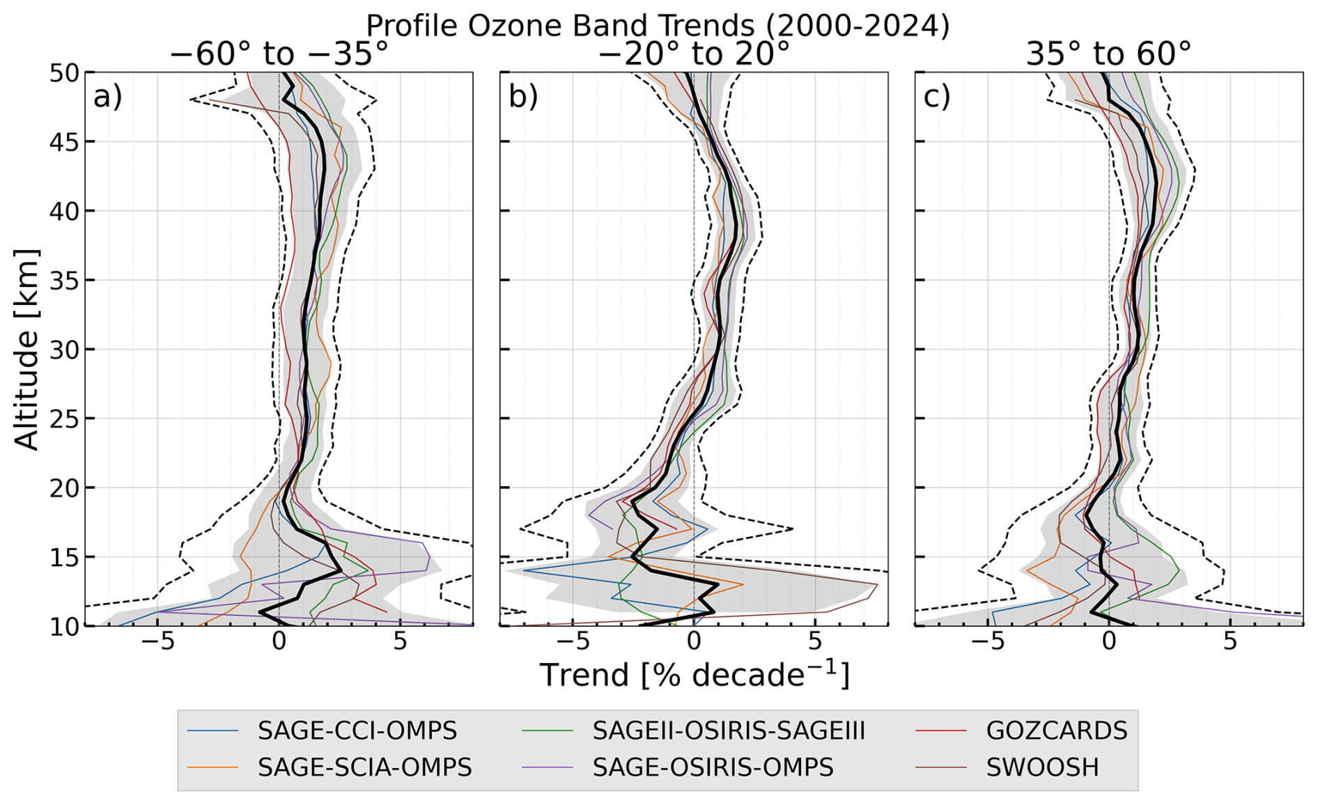
Figure A7 Ozone trends with the Full Regression Model from 2000 to 2024 in three distinct latitude bands ((a) 35–60° S, (b) 20° S–20° N, (c) 35–60° N) in % per decade for the six merged ozone profile datasets: GOZCARDS, SAGE-CCI-OMPS, SAGE-OSIRIS-OMPS, SAGEII-OSIRIS-SAGEIII, SAGE-SCIA-OMPS, and SWOOSH. Shaded area indicates the 2σ uncertainties, calculated using the LOTUS (Eq. 7) and the dashed line indicates the J-Distribution uncertainty (Eq. 9) of the mean trends (black line). Same as Fig. 10, but trends in units of % per decade.

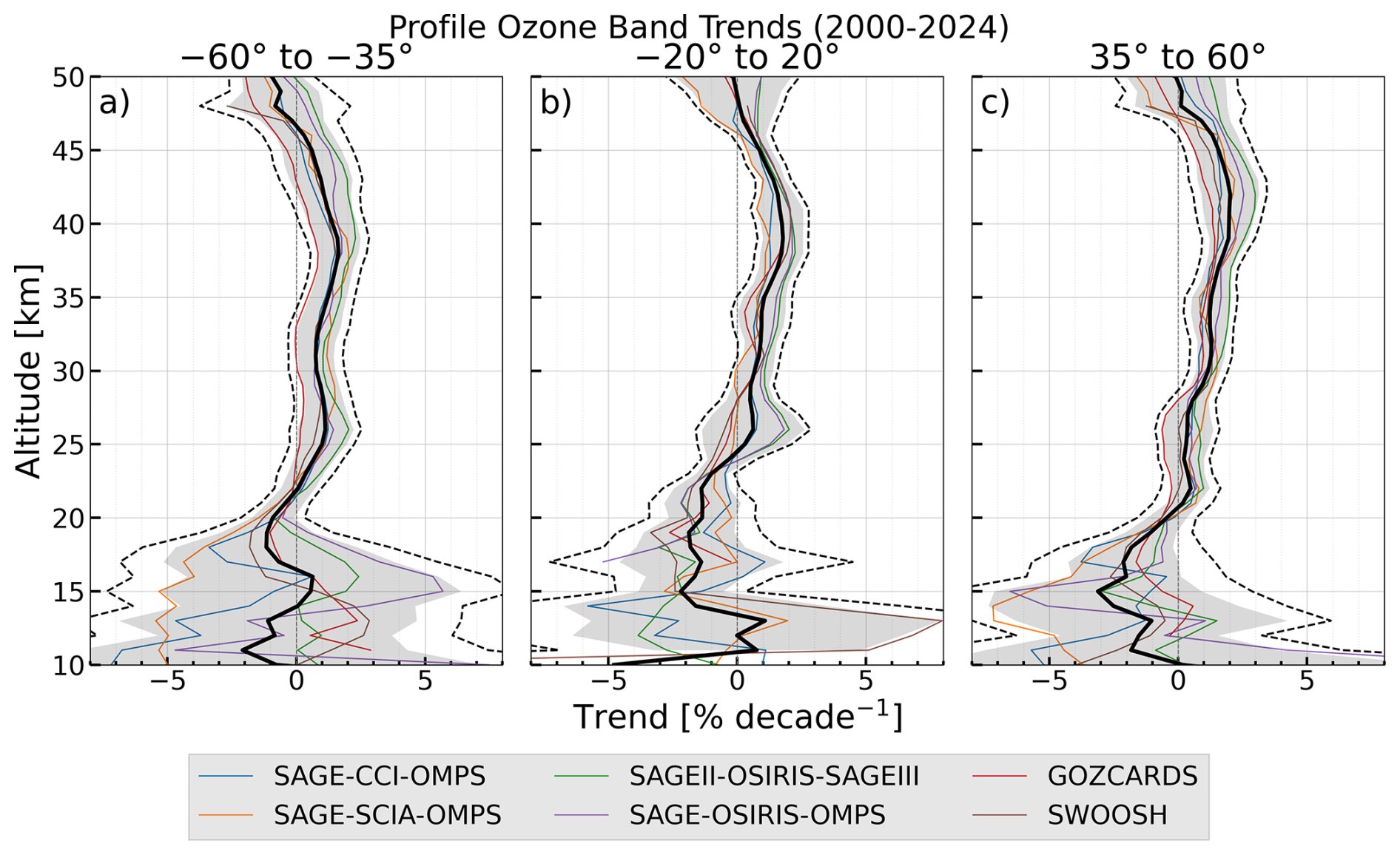
Figure A8 Ozone trends with the LOTUS Model from 2000 to 2024 in three distinct latitude bands ((a) 35–60° S, (b) 20° S–20° N, (c) 35–60° N) in % per decade for the six merged ozone profile datasets: GOZCARDS, SAGE-CCI-OMPS, SAGE-OSIRIS-OMPS, SAGEII-OSIRIS-SAGEIII, SAGE-SCIA-OMPS, and SWOOSH. Shaded area indicates the 2σ uncertainties, calculated using the LOTUS (Eq. 7) and the dashed line indicates the J-Distribution uncertainty (Eq. 9) of the mean trends (black line). Same as Fig.  10, but using the LOTUS setup in the MLR and trend units of % per decade.

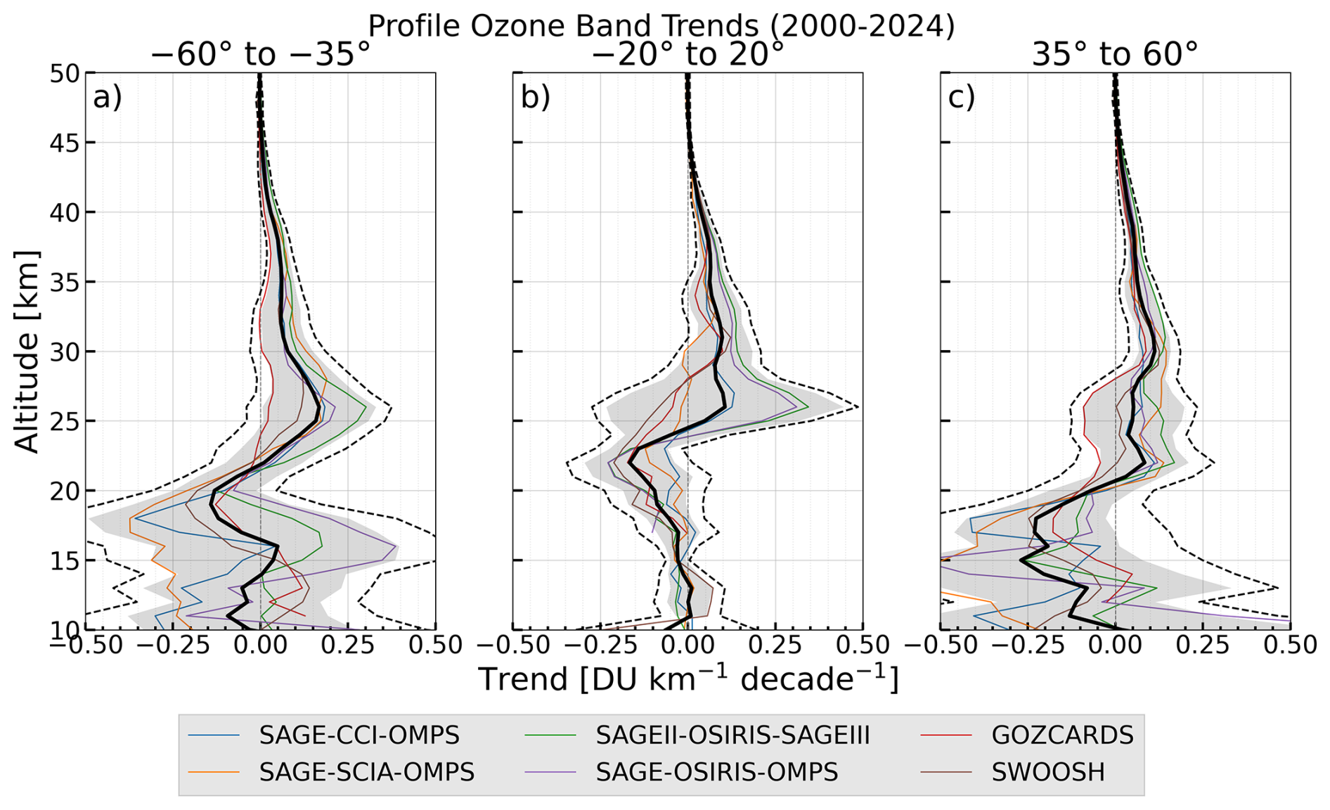
Figure A9 Ozone trends with the LOTUS Model from 2000 to 2024 in three distinct latitude bands ((a) 35–60° S, (b) 20° S–20° N, (c) 35–60° N) in DU km⁻¹ per decade for the six merged ozone profile datasets: GOZCARDS, SAGE-CCI-OMPS, SAGE-OSIRIS-OMPS, SAGEII-OSIRIS-SAGEIII, SAGE-SCIA-OMPS, and SWOOSH. Shaded area indicates the 2σ uncertainties, calculated using the LOTUS (Eq. 7) and the dashed line indicates the J-Distribution uncertainty (Eq. 9) of the mean trends (black line). Same as Fig. 10, but using the LOTUS setup in the MLR.