A cross-instrument closure and polarimetric study for improving sub-millimeter polarimeter-radiometer ice cloud microphysics retrievals

Ice cloud microphysical properties, such as phase, shape, size and density, introduce significant uncertainties and biases that affect our understanding of how clouds influence weather and climate. The upcoming spaceborne sub-millimeter radiometers are expected to help in reducing the ice microphysics induced uncertainties in observations. Yet our knowledge about ice microphysics in this spectrum is still limited, and comparison/validation work is still sparse.

This paper delivers a comprehensive cross-instrument closure study using active, passive remote sensing and in-situ cloud probe measurements collected during the NASA's IMPACTS field campaign. Through combined use of two radars, one lidar and in-situ cloud probe measurements, a comprehensive best reference “truth” is generated, which is then used to validate collocated sub-mm CoSSIR radiance measurements. We found out that only through a realistic vertical hydrometeor type classification that all types of measurements can reach a closure with minimal discrepancies between simulations and observations, which is critical for generating high-quality retrievals for frozen hydrometeors.

We further present a comprehensive exploration of the scientific merit of polarimetric measurements in improving frozen hydrometeor microphysics retrievals. For the first time, we can validate previous theoretical predictions that sub-mm polarimetric signals can be used to retrieve ice particle habit and size. Moreover, we find it is possible to differentiate detailed vertical structure of hydrometeor types using both polarimetric and radiance measurements. This paper paves concrete steps in assuring timely delivery of high-quality science products for the sub-mm radiometer missions as well as possibilities of new science products beyond the mission requirements.

1 Introduction

Ice clouds play a critical role in Earth's radiation budget and hydrological cycle. However, they are poorly observed by satellite remote sensing and poorly constrained in models too. Hence, their impacts on climate and weather come along with the largest uncertainties among all recognized forcings in the IPCC AR6 report (Pathak et al., 2022). From satellite remote sensing perspective, obstacles refraining us from retrieving accurate ice cloud parameters can be summarized in three manifolds: (1) cloud ice microphysical properties usually contain too many degrees of freedom; sub-footprint variabilities exacerbate this ill-posed retrieval problem; (2) cloud ice size spectrum spans such a wide range, and some parts of this spectrum have significant gaps that traditional remote sensing instruments cannot provide enough information about (Wu et al., 2024); (3) other than the small non-precipitating portion of the spectrum that is well sampled by instruments on the geostationary (GOES) platforms in both time and spatial domains, frequent observations for the medium to large sized ice particles that interact with convections and precipitations are lacking from space platforms, which largely impede the investigation of the cloud-convection-precipitation (CCP) coupling processes.

Sub-millimeter (sub-mm; 183–840 GHz) is an ideal spectrum range for observing the medium-large sized ice particles. For one, the depression of measured radiance in this spectral regime is dominated by ice scattering because of insensitivity to liquid emission and surface emission due to water continuum; for two, unlike visible band which is daytime only, sub-mm can continuously monitor the medium-large size range both day and night without relying on multiple scattering to penetrate deeper into clouds; and thirdly, ice scattering signal at sub-mm band is more sensitive to details of the ice microphysical properties compared to passive microwave (PMW) instruments (e.g., Ekelund et al., 2020). As a proof-of-science concept and technology readiness, the launch of a cubesat mission IceCube demonstrated the high science value of using sub-mm bands to fill in the observational gap between infrared (IR) and PMW bands (Gong et al., 2021; Wu et al., 2024).

Several spaceborne sub-mm radiometers are in the pipeline for launch in the next few years. These include European Space Agency (ESA)'s Ice Cloud Imager (ICI), NASA's Earth Venture class mission Polarized Submillimeter Ice Cloud Radiometer (PolSIR), France's Convective Core Observations through MicrOwave Derivatives in the trOpics (C²OMODO) as part of NASA's Precipitation Measurement Mission (PMM). The latter two missions will be on processing orbits to sample the full diurnal cycle of ice clouds in the tropics and sub-tropics, while ICI will be flying on a polar-orbiting Sun synchronized orbit. As the pathfinder of EUMETSAT Polar System Sterna constellation (EPS-Sterna) and the first operational sub-mm mission, the Arctic Weather Satellite (AWS) was launched in 2024, and the Level-1 and -2 data are showing high scientific quality. A sizable amount of independent validation efforts have also been carried out using airborne version sub-mm radiometers (e.g., Evans et al., 2005; Fox et al., 2019).

High sensitivity to ice microphysical properties is a double-edged sword for sub-mm bands. It translates into larger uncertainties in the ice cloud retrieval products for sub-mm radiometers as assumptions of ice microphysical characteristics would cause larger downstream impacts. Previous studies have demonstrated that polarimetric signals can help significantly in constraining some of the ice microphysics assumptions and reducing retrieval errors by ruling out certain incorrect microphysics assumptions (Gong and Wu, 2017), by explicitly incorporating the statistical effects in the retrieval process (Kaur et al., 2022), or by enabling direct retrievals of some microphysical properties (McCusker et al., 2024). ICI and PolSIR instruments will be equipped with polarized channel pairs to take polarimetric measurements for certain channels. While radiative transfer simulations have been carried out at research level to understand the observed relationship between polarimetry and ice microphysics (Gong and Wu, 2017; Brath et al., 2020; Battaglia et al., 2011; Wu et al., 2024), validation work remains nearly non-existing due to the lack of in-situ or ground reference microphysics measurements at this spectrum. McCusker et al. (2024) is the pioneer and the only one to our best knowledge that employed cloud probe measured ice habits and particle size distribution (PSDs) and Ka-band radar derived hydrometeor mass profiles to simulate the observed polarimetric signal at 243 GHz by ESA's airborne sub-mm simulator ISMAR (International Sub-Millimetre Airborne Radiometer). Limited by the campaign payloads and flight pattern, this work has some inevidible caveats which will be discussed later in this paper for a latitudinal comparison, but this is the first closure study demonstrated that passive polarimeter-radiometer and active radar observations cannot reach high-level agreement without including proper frozen hydrometeor microphysics assumptions, and this is the pioneering work that inspired our study.

This paper executes a comprehensive, multi-faceted research framework organized around three inter-linked objectives. The first objective stresses the criticality of cross-instrument consistency about ice microphysics properties, and the other two objectives further explore the scientific utility of multi-channel sub-mm polarimetry in better retrieving the vertical hydrometeor phase distribution and ice particle size. By linking a strict active/passive/in-situ closure study with targeted polarimetric applications, this work aims at establishing concrete baseline protocols for optimizing the operational/research science products of upcoming spaceborne sub-mm radiometer missions.

This paper is organized as follows. In Sect. 2, we will present the datasets/database and methodology, Sect. 3 on results, Sect. 4 on a discussion and last section on summary and future plans.

2 Datasets and Methodology

2.1 Case and payloads description

For this validation and closure study, the radiance and polarimetric observations come from the CoSSIR (Configurable Scanning Submillimeter-wave Instrument/Radiometer) onboard the NASA IMPACTS (Investigation of Microphysics and Precipitation for Atlantic Coast-Threatening Snowstorms) campaign ER-2 aircraft, which was cruising at >16 km altitude during operational mode (i.e., above winter weather systems). Other payloads on the same aircraft include a W-band radar (CRS), a dual-frequency Ku/Ka band radar (HIWRAP), and a multi-frequency cloud physics lidar (CPL; McGill et al., 2002). We will use these three active sensor measurements jointly to provide the best estimates of frozen hydrometeor types and their vertical distributions for the subsequent CoSSIR retrieval of ice water path (IWP) and mass-weighted effective diameter (D_me). The retrieved size parameter will then be compared with in-situ cloud probe measurements from the co-flying P-3 aircraft at a lower altitude (∼ 5–7 km) that co-incides with the channel response function peak altitude of 325±11 GHz. More detailed information and datasets about this campaign can be found in McMurdie et al. (2022) and Yorks et al. (2025). Due to the sparseness of dropsondes, the NOAA high-resolution rapid refresh analysis (HRRR) temperature and water vapor profiles are used to represent the ambient and in-cloud thermodynamic structures for our combined active-sensor hydrometeor type classification, and the Weather Research Forecast (WRF) simulations generated atmosphere is used for forward radiative transfer simulation, both of which admittedly contain errors and biases that are difficult to identify.

Data collected during 16:00–18:30 UTC on 15 January 2023 is used for this validation work. Please note that all time labels in figures throughout this paper express time in decimal hours (e.g., 16.75 UTC = 16:45 UTC). The flight trajectories during this period sampled multiple times through the shallow warm-core intensitification phase of a Western Atlantic oceanic cyclone, as shown in Fig. 1. A consolidated surface low first appeared at 00:00 UTC on 15 January off the North Carolina coast (37° N, 70° W). Then between 06:00 UTC and 12:00 UTC the cold core migrated to warm core, and the shallow surface warm core structure intensified afterwards. Because of the warm core and sea surface temperature (∼22 °C), one can see strong melting band and consistent rainfall below from Fig. 1d, e and f for W-band radar reflectivity curtains. Above the melting band, different frozen hydrometeors are observed in situ by the CPI (cloud particle imager) onboard the P-3 aircraft. At 16:11 UTC, there were mostly ice plates or ice columns. At 17:12–17:18 UTC when the P-3 flew through the cyclone center from southwest to northeast at the same altitude, CPI captured large plate aggregates at the west side but mostly mixed-phase or ice pellets at the east side (Figs. 10 and 12 in McMurdie, 2025).

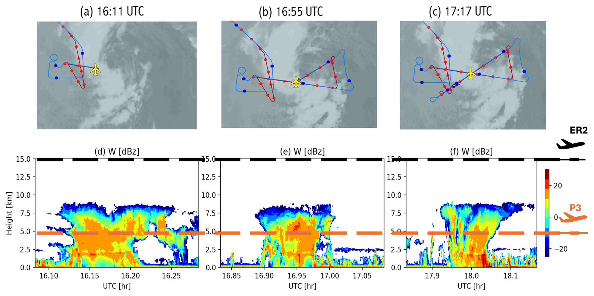
Figure 1 Illustration of the weather system and flight patterns of the 15 January 2023 IMPACTS campaign case. Top rows are ER-2 (blue) and P-3 (red) flight routes overlaid on GOES-16 satellite false-color Advanced Baseline Imager (ABI) albedo measurements at three different UTC times. Dots mark the time at intervals of 5, 10, 15 min, and so on. Cyclone center was roughly at 37° N, 70° W. Bottom row presents the CRS radar reflectivity curtains during the corresponding time segments. Two aircraft icons roughly represent ER-2 and P-3 flight altitudes. Top panels are cropped from https://catalog.eol.ucar.edu/maps/impacts_2023 (last access: 26 June 2026), and bottom panels are calibrated L1B CRS W-band radar reflectivities at corresponding periods. GOES-16 ABI data courtesy of NOAA. NCAR/EOL map products courtesy of NCAR/UCAR. CRS radar data courtesy of NASA.

Because the 15 January flight is an atypical case for the IMPACTS campaign, which means the hydrometeor types and vertical distributions could be quite different from the rest winter storm cases sampled during this three-year long campaign, we selected a 5 February case and applied the same strategy to obtain the reference hydrometeor types (see next subsection for methodology). This case was then used for the training task later to test the robustness of our hydrometeor classification algorithm. 5 February was a typical winter frontal system. During 15:00–18:00 UTC, both flights sampled through the warm front sector latitudinally. This warm front was fairly shallow with core mostly below 4 km and absence of the melting band. Plates, columns and their aggregates were consistently observed during this 3 h period (McMurdie, 2025).

2.2 Reference Dataset Generation

2.2.1 Hydrometeor type classification using a combination of radars and lidar

A combined triple-frequency radar (CRS+HIWRAP) + CPL lidar multi-head decision tree method is developed to separate the hydrometeors into five coarser classes (clear-sky, liquid, supercooled liquid, mixed and ice) and to further break down the ice into 5 more detailed categories (ice, small ice, unrimed aggregates, rimed aggregates, and graupels). This algorithm is an updated version of Finlon et al. (2022) and Tridon et al. (2019) by adding-in lidar signals in determining the hydrometeor type at the cloud tops and identifying supercooled liquid layers (SCLW), the thresholds of which are determined by the in-situ cloud and precipitation probe measurements. An example of such dynamic varying thresholds for CPL is shown in the colored panel in Fig. 2. We first identify the P-3 altitude and corresponding collocated and coincident CPL observations. Then the CPL depolarization-backscatter measurement is then assigned into liquid, ice or mixed-phase class by comparing with an independent Rosemont Icing Detector (RICE) instrument onboard the P-3 aircraft (Cober et al., 2001). RICE's vibration frequency is sensitive to cloud particle phase, especially to SCLW (Finlon et al., 2025). For each campaign deployment day, a probability distribution of different hydrometeor phases is constructed using all the collocated CPL-RICE samples, from which we can draw the two partitioning lines in the depolarization ratio (δ₅₃₂) and backscatter (β₅₃₂) diagram. These two dividing lines are used as the thresholds for determining the hydrometeor phase when CPL is used. The SCLW layer is then further separated from liquid phase using the 0 °C temperature threshold. For every vertical profile, the classification procedure always starts from the cloud top and CPL observations. Once the CPL signal saturates, CRS reflectivity is then used together with HRRR temperature to determine cloud phase. We employed a similar temperature threshold that CloudSat 2B-CWC-RO algorithm uses to define a relatively broad temperature range (−30 °C $<T<\mathrm{0}$ °C) to allow mixed-phase to exist. However, once reaching the altitude when HIWRAP-Ku band measurement passes its minimal detection threshold, HIWRAP observations take the decision over as dual-frequency are much less ambiguous at hydrometeor type defferentiation than a single-frequency (CRS) radar reflectivity measurement. For HIWRAP data, we follow the Tridon et al. (2019) method to mainly rely on the riming parameter and 0 °C temperature threshold for phase determination (Fig. 2a). For a certain altitude if both CRS and HIWRAP do not receive significant enough radar echo return, this altitude and location is classified as “undefined”, corresponding mostly to clear-sky range bin. The riming parameter (r) is defined as: $r=\mathrm{0.05}{Z}_{\text{Ku}}-\mathrm{0.25}{\text{DWR}}_{\text{KuKa}}^{\mathrm{0.5}}-\mathrm{0.3}$. Using r, temperature and minimal HIWRAP-Ku band minimal detection threshold of 15 dBZ, we then further break down the frozen hydrometeor into 5 more categories as illustrated in Fig. 2b. In reality the “small ice” that Ku-band misses but Ka-band detects probably overlaps with the “ice” category that CRS detects, but we still separate them into two different categories for now to avoid potential inconsistency. The last “melting ice” category only happens in the melting layer (i.e., “bright band” zone). For the forward simulation and retrieval steps, this category is completely ignored as no radiative transfer models (RTMs) can handle the melting layer radiative transfer satisfyingly.

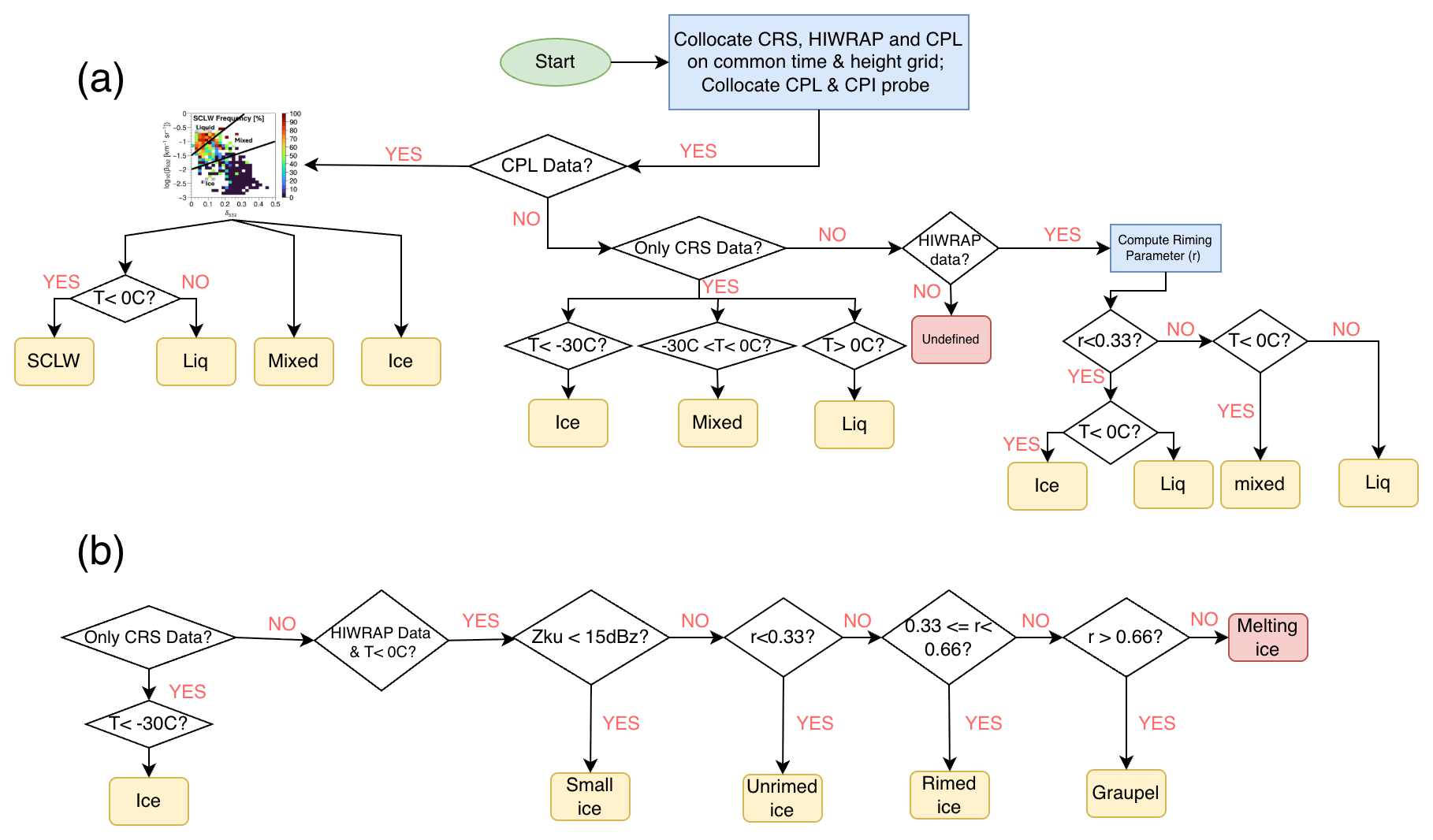
Figure 2 (a) Decision tree for the coarser 5-class hydrometeor classification using CRS,HIWRAP and CPL; (b) further decision tree for finer classification among the ice category. Blue rectangles enclose computing procedures; yellow rectangles enclose the final output categories while pink rectangles are either undefined or not considered in further analysis.

Figure 3 gives an example curtain sampled during one flight leg that crossed the cyclone core between 17:12–17:36 UTC on 15 January 2023. We can clearly see that CPL and CRS together fill in the missing convective cloud top layers between 6–8 km, the stratiform rainfall band below 2 km and the outskirt of the convective cloud that HIWRAP would miss to reveal. On the other hand, both CPL and CRS clearly saturate and can not see through the core, while HIWRAP-Ku band can (Fig. 3c), and the riming parameter (Fig. 3d) suggests significant riming processes happening within the core (r>0.33). In addition, we can identify from decreased lidar depolarization ratio (Fig. 3a) the mixed-phase pockets embedded in the convective cloud top ice layer, as well as the SCLW layer between 17:20–17:30 UTC at ∼2.5 km. Readers should also be aware that our final cloud phase products (Fig. 3e and f) ignore the melting layer, which should be present in the convective core between mixed-phase cloud and liquid precipitation. We also want to make clear that there are additional radar measured Doppler velocities that could have been employed to further help improve the hydrometeor type classification. This could become one of our future efforts but not included in this current algorithm.

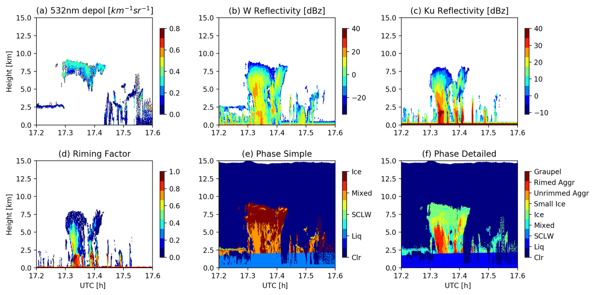
Figure 3 An example to show how the final hydrometeor type is decided based on (a) lidar 532 nm depolarization ratio (δ) and backscatter (β; not shown); (b) W-band reflectivity; (c) Ku-band reflectivity; and (d) calculated riming parameter (r). The final coarse and detailed type classification products are shown in (e) and (f), respectively.

2.2.2 IWC and LWC Reference Profile Generation

With knowledge of this refined vertical hydrometeor type information, we can then retrieve the vertical profile of hydrometeors and particle size using the classical optimal estimation method (OEM) approach. At each altitude, the goal is to minimize the cost function, defined as the sum of the normalized reflectivity difference between observation and forward simulations plus the normalized apriori difference:

$$\begin{array}{}\text{(1)}& S={\mathrm{\Sigma }}_{i=\text{W,Ka,Ku}}{\displaystyle \frac{(R_{\text{obs},i}-R_{\text{simu},i}{)}^{\mathrm{2}}}{{\mathit{\sigma }}_i^{\mathrm{2}}}}+{\displaystyle \frac{(x-x_{\mathrm{a}}{)}^{\mathrm{2}}}{{\mathit{\sigma }}_{\mathrm{a}}^{\mathrm{2}}}}\end{array}$$

The radar OEM retrieval follows the method detailed in Liu et al. (2022). With a pre-calculated IWC-reflectivity database, an onion-peeling method is performed in which Monte-Carlo Integration is applied to each reflectivity layer from the top downward, and the resulting radar attenuation is used to correct the radar reflectivity below. The mean and standard deviation obtained at each layer are then used as the a priori state x_a and its uncertainty σ_a during the OEM process. The state x_a is also used as the initial guess for the OEM.

Very few radiative transfer models (RTMs) can handle the complicated scattering computation from ice particles with different shapes at MW to sub-mm frequencies. For our work, we employ the Atmospheric Radiative Transfer Simulator (ARTS) that is well acknolwedged to be one of the best at ice scattering simulation for MW to sub-mm bands (Buehler et al., 2018). ARTS incorporates a sophisticated ice scattering database that has been used as a benchmark for other RTMs (Barlakas et al., 2022) and validated against several spaceborne (sub-)mm radiometer observations (e.g., Ekelund et al., 2020; Gong et al., 2021; Eriksson et al., 2025). It allows users to select from 34 ice habits and 7 PSD options (Eriksson et al., 2018) so suitable to handle the complicated refined ice types in our study. ARTS also incoorporates the land surface emissivity model TELSEM² (Tool to Estimate Land Surface Emissivity from Microwave to Submillimeter Waves) and ocean surface emissivity modelTESSEM² (Tool to Estimate Sea-Surface Emissivity from Microwaves to sub-Millimeter waves), both have been validated in the sub-mm regime up to 325 GHz (Prigent et al., 2017; Wang et al., 2017) and are used in our case study as this cyclone is over ocean, and the 5 February case is over land. The discrete ordinate iterative (DoIT) solver is employed for non-polarized RT calculations considering its high accuracy, and the RT4 solver is used for polarized RT calculation considering its high computation efficiency and it has been validated against satellite observations (Gong and Wu, 2017). We assumed 1D atmosphere and independent beam approximation (IBA), which would introduce a negligible low bias to simulated brightness temperatures (TBs) for CoSSIR according to Barlakas and Eriksson (2020). CRS range bin resolution of 25 m is employed for RT model vertical resolution with a total of 609 vertical layers.

As the ice habits provided in ARTS model do not necessarily match our refined categories, we use “large column aggregates” (LCA) in ARTS to represent “ice”, “Evan's snow aggregates” (ESA) for “small ice” and “unrimed aggregates”, “graupel” for “rimed aggregates” and “graupel”, and “spherical liquid” for “liquid (including liquid cloud and rain)”, respectively. Because of the challenge of simulating radiative transfer in melting layer, we focus on only retrieving ice water content (IWC) and liquid water content (LWC) in our current study and ignoring finding the best solution for melting layer. A single-moment PSD from Field et al. (2007) for mid-latitude scenario is assumed everywhere to project retrieved IWC (LWC) to D_mei (D_mel).

2.2.3 Independent cloud probe observations

In addition to check the consistency among active and passive sensor measurements, two types of additional in-situ cloud probe observations are also used. One is the Rosemont Icing Detector instrument (RICE), the instantaneous vibration frequency of which is used for building the thresholds for CPL to differentiate liquid, SCLW, ice and mixed-phase. RICE is sensitive to particles with effective diameter (D_e) between 25 to 1550 µm (Cober et al., 2001). RICE has an oscillation probe with a sensing cylinder in the middle. When ice builds up on the sensing cylinder, the oscillation frequency changes subsequently, which is related to the rate of ice accretion (Finlon et al., 2026). The other one is called 2D-S stereo probe, which is used as the independent validation for IWC from radar retrievals and D_me from radiometer retrievals. It's particle diameter sensitivity range is 10 to 1280 µm (Lawson et al., 2006, 2008). Diffferent from RICE which has no capability of telling particle shape nor orientation, 2D-S switches between side-view (H-channel) and birds-eye-view (V-channel) to detect the area of particles that obscuring the sample volume using a laser beam, hence the retrieved particle shape, size and PSD could be quite different from different views. In our work we use the D_me and IWC retrieved from the V-mode images as this view should provide the most accurate measurement of particle size, shape and size distribution for dominantly horizontally oriented frozen particles.

Even though cloud probe observations are used as the “in-situ truths” to validate remote sensing retrievals, which is a widely adopted approach by many other prior research (e.g., McCusker et al., 2024), the images essentially lack mass (or density) information to associate particle size with IWC and D_me. In other words, The latter two variables are also “retrieved” for in-situ measurements with some assumption of the mass-size (m–D) relationship. In this work, three m–D assumptions are employed when conducting the independent validation, which are based on Brown and Francis (1995), Chase et al. (2021) and Heymsfield et al. (2010). Furthermore, cloud probe image frame size is on the order of mm with resolution of ∼2.5 µm, while CPL, CRS, HIWRAP-Ka, HIWRAP-Ku and CoSSIR footprint size are 1 m, 150 m, 400 m, 1 km and 1.1 km (nadir), respectively. Such a huge disparity in measuring dimension means that comparing in-situ and remote sensing retrievals directly requires homogeneity of microphysics across several hundred meters horizontally, which is unlikely the case for most of the time. These are caveats that are inevitable and should be made clear up-front that the associated errorbar is unquantifiable and beyond our scope of this study.

2.3 CoSSIR and Polarimetric Measurements

Currently there are two airborne sub-mm polarimeter-radiometers worldwide that are used as satellite simulators for the current and upcoming spaceborne sub-mm radiometers: ISMAR developed by UK Met Office and ESA (Fox et al., 2017), and CoSSIR developed by NASA (Evans et al., 2005). The latter was deployed during the CRYSTAL-FACE (Cirrus Regional Study of Tropical Anvils and Cirrus Layers, Florida Area Cirrus Experiment) and TC4 (Tropical Composition, Cloud and Climate Coupling) campaigns, both were in deep tropics. It was then reconfigured to add polarization to all frequencies, updated with a new receiver and a stand-alone pedestal (Kroodsma et al., 2024). The new CoSSIR channel frequencies and noise levels can be found in Table 1. During the January–March, 2023 IMPACTS campaign, CoSSIR was operated under three modes: forward conical scan at a fixed scan-angle of 52.8°, cross-track scan, and along-track scan.

Table 1 CoSSIR channel frequencies, bandwidths and noise equivalent differential temperature (NEdT). 182.3 V and 325±0.9 V are excluded for this study due to calibration issues.

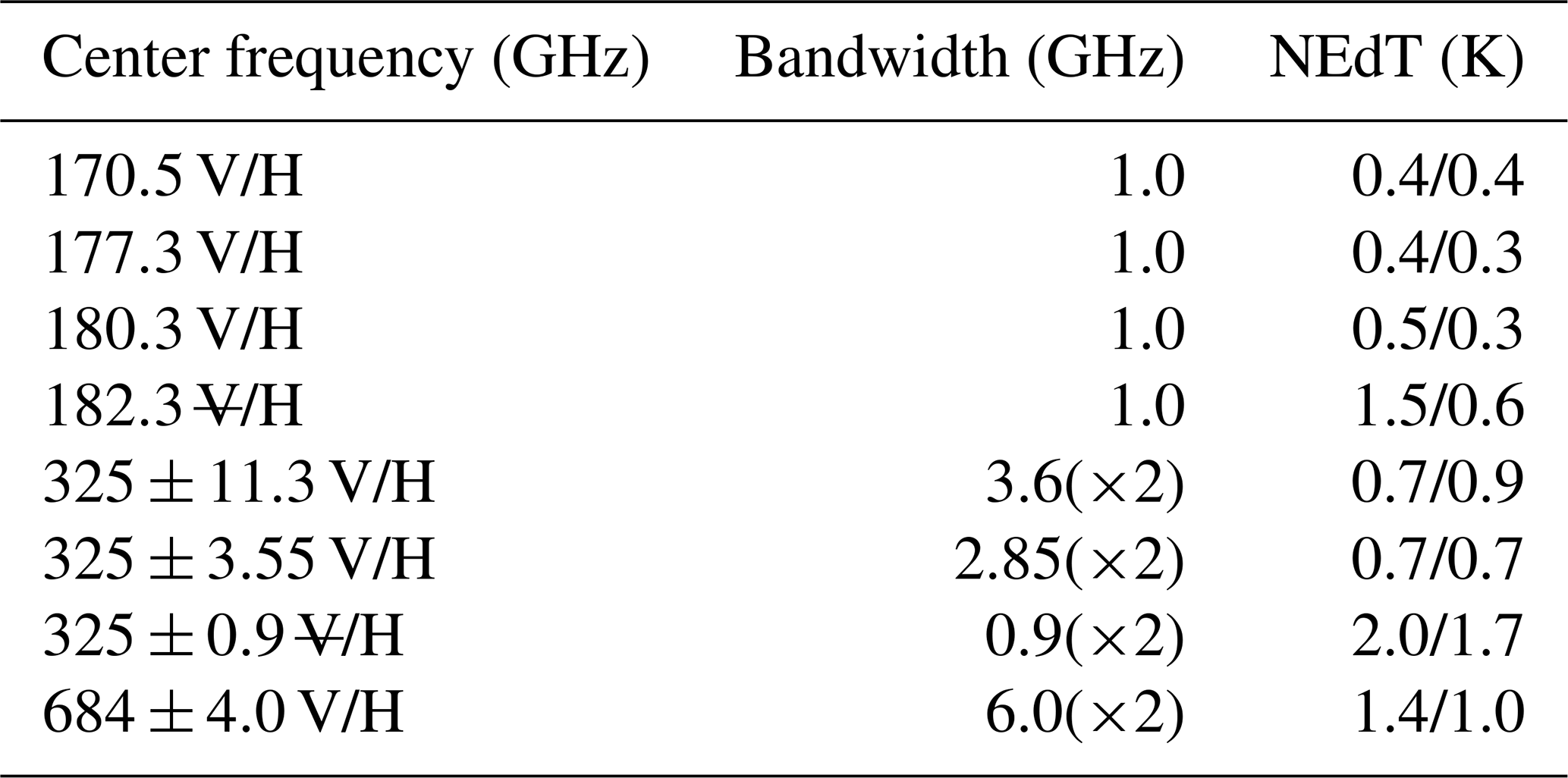
For this closure study, we do not perform direct retrieval using CoSSIR multi-channel radiance measurements. Rather, the IWC and LWC retrieved from the triple-frequency radar algorithm are the inputs fed into the forward model to compute simulated radiance and compare with observed ones to check consistency and sensitivity to ice microphysics. Same microphysics assumptions with radar retrieval algorithms are used for the radiometer forward simulation.

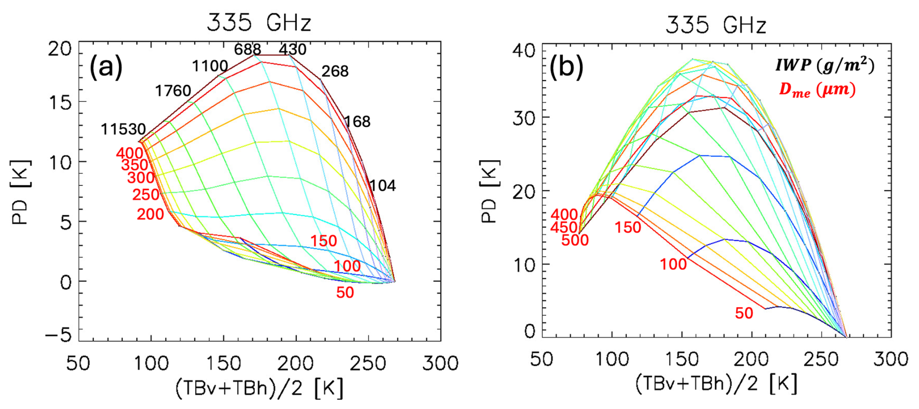
As Gong and Wu (2017) and Wu et al. (2024) have demonstrated that the PD–TB relationship (PD stands for polarization difference, which is defined as TB_V−TB_H from the same frequency channel pair) for a specific frequency is a function of both IWP and D_me using fully polarized radiative transfer simulations, we can use the look-up-table (LUT) approach to identify the best D_me and IWP pairs in the solution space that minimizes the Eucledian distance to the observed TB and PD from single frequency measurements. Barlakas et al. (2021) and Brath et al. (2020) have demonstrated previously that PD is insensitive to the degree of ice particle orientation at scan angle of 52.8°. Hence, using data from this special view-angle can help eliminate the assumption of 100 % horizontal orientation when constructing the LUT, which is an unrealistic assumption in most realworld cases. Avoiding making this assumption is a critical step in assuring robustness of the retrieval results. In this study we therefore only employ CoSSIR measurements from the conical scan mode or cross-track mode with scan angle between 50 and 55° whenever the aircraft is above 16 km (i.e., well above the highest cloud top in this case). Data collected during large yaw, pitch or roll angles are also excluded to avoid cross-polarization information leaking. Strictly speaking, the LUT is also a dependent of ice habit (Brath et al., 2020). In our work, we assume two types of representative ice habit when generating the LUT: 6-bullet Rosette to represent the snowflakes, and column ice to represent small ice crystals. The RT4 solver is used for this fully polarized RT simulation (Gong and Wu, 2017). To make sure the uniform habit assumption is not severely violated, we also exclude convective zones by checking the existence of a melting layer. Filtering out convective scenes help mitigate the inhomogeneity issue mentioned above when we compare CoSSIR retrievals against in-situ cloud probe reference.

2.4 Framework for Closure and Polarimetric Study

This study consists of three main objectives, covering two subjects, and the corresponding approach is shown in the flow chart in Fig. 4. The first objective is a closure study, as enclosed by the pink patched area in Fig. 4. We will be using the same set of hydromteor type profiles for CRS plus HIWRAP radars to retrieve the IWC and LWC profiles, which will be checked against radar reflectivity measurements using the ARTS radar simulator. The retrieved IWC profiles will be validated against independent 2D-S IWC retrievals at P-3 aircraft cruising level. The retrieved hydrometeor mass and particle size profiles will then be fed into the forward model with the same set of hydrometeor type profiles to generate simulated brightness temperature (TB), which will be compared against CoSSIR observations. Uniform habit assumption throughout the scene will be employed as the sensitivity test to understand how sensitive the cross-instrument consistency is to ice particle shape. However, PD measurements are not considered in this entire closure study task.

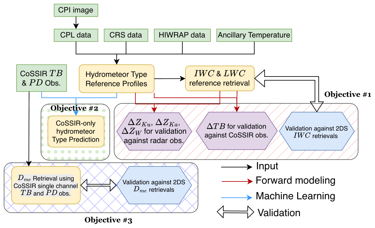
Figure 4 Architecture flow for this work. Green rectangles are observations (or ancillary atmospheric field) as retrieval or machine learning inputs. Yellow rectangles are retrieval products from this work, purple hexagons are consistency check as part of the closure study, and blue hexagons are independent validation from in-situ 2D-S cloud probe observations as the other part of the closure study. Red arrows represent forward modeling operator to convert physical parameters to remote sensing variables. Blue arrows represent the machine learning task. This paper includes three objectives, which are enclosed by the pink hatched area, green dotted area, and blue cross-hatched area, respectively.

The other two objectives explore the subject about how the additional information from PD can constrain microphysics. For the 2nd objective (green dotted area), we will conduct a machine learning task to train CoSSIR to predict the vertical hydrometeor type distribution. PD will first be excluded in the baseline model and then added to evaluate the improvement. For the last objective (blue cross-hatched area), PD will be used together with TB to retrieve ice particle size, which will then be validated against independent 2D-S D_me retrievals. Because both tasks rely on retrieval products generated from the first task, and both include an independent validation step (for Objective #2, the validation follows standard ML protocol), these two objectives fit under the closure-study umbrella in a broader sense.

3 Results

3.1 Closure Study

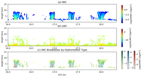
The radar retrieved IWC and LWC profiles between 16:00–18:30 UTC are shown in Fig. 5. During this 2.5 h period, the two aircrafts passed the cyclone center 4 times. However, if we only have IWC retrieval without breaking it down into more detailed hydrometeor types, as shown in Fig. 5a, it is almost impossible to tell how the cyclone changed over this period. When we have more detailed vertical information (Fig. 5b), we can see this cyclone center was still developing at ∼ 16:12 UTC given a core occupied by graupel and large graupel IWC values. Scattered single convective towers in the vicinity also suggested developing phase. At ∼ 18:00 UTC, the storm center was filled with snow aggregates and decreased IWC values. Stratiform mixed-phase low-level clouds at ∼3 km started to be captured when the aircrafts passed the storm the second time (∼ 17:00–17:12 UTC). Such a layer also indicates saturation and decaying of this cyclone, accompanied by periodic rainfall. After 18:00 UTC when the aircrafts passed the center the 4th times, the stratiform rain layer became quite evident. It is also quite interesting to see positive LWC (i.e., mixed-phase clouds) consistently appearing at the convective cloud top throughout this 2.5 h period, which is certainly SCLW, and they are mostly unambiguously determined by the CPL depolarization ratio. Although there was unfortunately no in-situ cloud probe observations at ∼10 km to validate these SCLW cloud, they were repeatedly reported in cold cloud systems by previous aircraft measurements. Rauber and Tokay (1991) attributed this unique SCLW scenario to the imbalance between the large condensate supply rate by strong updraft and the relatively slow ice crystal growth rate because they are small there as well as radiative cooling at cloud top, while Rosenfeld and Woodley (2000) provided a similar explanation, but attributing the latter to the lack of ice nuclei there. Moreover, Zaremba et al. (2024) found 19 % of of IMPACTS campaign cloud scenes appeared to have SCLW on the cloud top, again demonstrating the ubiqutous existence of SCLWs. Our work seems to lean toward supporting the explanation by Rosenfeld and Woodley (2000) more, because the updraft evidently became weaker at later stage of this studying period, yet the SCLW layer at the cloud top still sustained. As both CRS and HIWRAP are Doppler radars, the vertical velocity measurements should be explored in the future to understand better of these SCLW clouds.

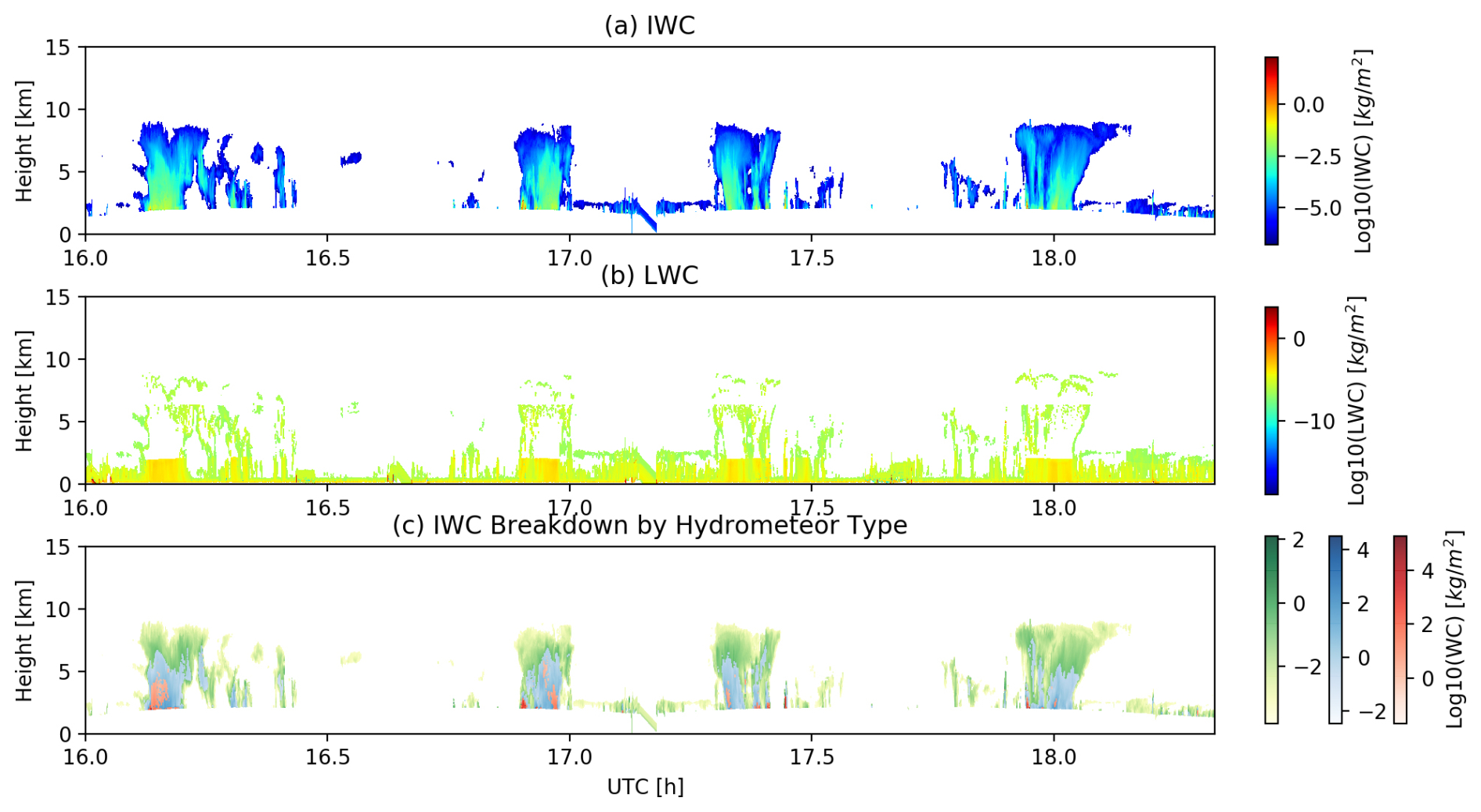
Figure 5 Vertical water content (WC) profile retrieved from CRS plus HIRWAP. (a) IWC; (b) LWC; (c) IWC from cloud ice (green), snow aggregates (blue), graupel (red) and liquid. Colorbars are in Log₁₀-scale. Note that positive LWC pixels overlap with many of the positive IWC pixels (e.g., cloud top, cloud boundary, SCLW layer, etc.), so they are shown separately in (a) and (b) to ease visual comparison.

Next we check the quality of hydromteor profile retrievals against real CRS and HIWRAP observations by using the ARTS radar forward simulator to convert the hydrometeor profiles to radar reflectivities. 17:00–17:48 UTC is the period picked for scrutinization. During this period, ER-2 flew from southwest toward northeast direction, hovered around the convective center for about 5 min, and returned along roughly the same trajectory. Therefore, it sampled both the southwest sector of this cyclone as well as the center. P-3 was arranged to consistently fly underneath the ER-2 with flight height from 5.4 km at 17:00 UTC to 3.5 km at 17:48 UTC. During this period, P-3 released 9 dropsondes, separated apart by ∼6 min.

The hydrometeor classification results are detailed in Fig. 3f. Reflectivity differences ΔZ (defined as Z_simu−Z_obs) are shown in Fig. 6a, b and c for Ku-band, Ka-band and W-band, respectively. Such an experiment is also carried out by assuming all frozen hydrometeors are graupel (Fig. 6d, e, and f) or LCA (Fig. 6g, h, and i). Note that when we conduct the latter two sensitivity experiments, the uniform ice habit assumptions were made during both the retrieval and forward simulation steps so that the microphysics assumption is maintained across-board and no additional ΔZ is introduced to bias our comparison. The bottom row displays the mean difference as a function of height, where segment below melting layer and above cloud top is excluded. Due to the expected challenge in simulating the melting layer, our LWC retrievals below is also likely biased, so we neglect discussing discrepancies within and below the melting layer and only focus on the frozen hydrometeors above. This is justified as our focus is CoSSIR essentially which is primarily sensitive to frozen hydrometeors.

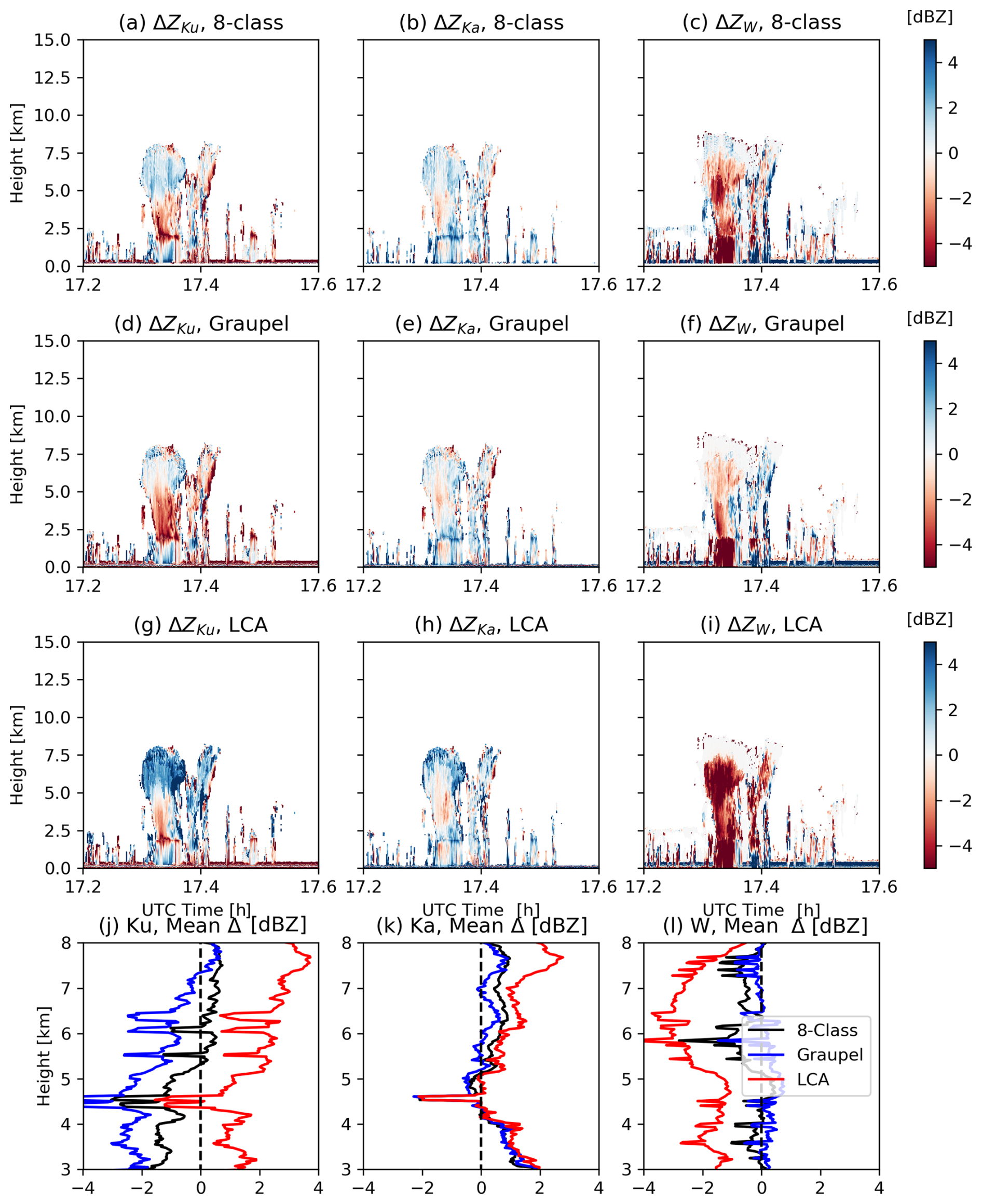
Figure 6 Reflectivity difference ΔZ between simulated and observed ones for HIWRAP-Ku (left), HIWRAP-Ka (middle) and CRS (right) using three different ice habit assumptions. The top row employs the three detailed ice class (LCA/ECA/Graupel), the middle row assumes graupel-only for all frozen hydrometeors and the 3rd row assumes LCA everywhere for all frozen hydrometeors. The bottom row shows the comparison of mean difference as a function of height for Ku, Ka and W band, respectively.

As one can clearly see, detailed hydrometeor information including mass and habit can effectively help close the gap between observations and simulations. Above the melting layer, $\left|\mathrm{\Delta }Z\right|<=\mathrm{2}$ dBZ mostly when detailed hydrometeor type is considered, although the simulated Z still tends to be on the smaller side within the graupel layer for Ku-band (Fig. 6j), and snow aggregates generated Z is low-biased as well for W-band (Fig. 6l). Assuming graupel everywhere produces slightly larger (smaller) negative biases in the convective core for Ku-band (W-band) compared to the results using detailed habits (Fig. 6j and l). The overall performance across three frequency bands are comparable, but we know graupel in anvil cloud deck is a rather irrational assumption. Assuming LCA everywhere introduces large positive biases (ΔZ>4 dBZ) in anvils for Ku-band large negative biases ($\mathrm{\Delta }Z<-\mathrm{4}$ dBZ) everywhere for the W-band except for the anvil cloud deck. This means ice particles in the assumption is too strong in scattering, which strongly suggests that LCA should not be the dominant habit within the convective cloud.

Thirdly, now we can also check whether the retrieved IWC with the detailed vertical hydrometeor types can reproduce the CoSSIR observed TBs. ARTS is again employed as the forward simulator to convert between physical variables and measured TBs. Auxillary inputs including temperature and water vapor profiles came from the WRF simulations. For sensitivity tests, whole-column LCA and whole-column graupel are again assumed for all frozen hydrometeors. We can clearly see that both 170.05 and 325.15±11.5 GHz are sensitive to ice particle habit (Fig. 7a and b). Using LCA assumption can only generate $\mathrm{1}/\mathrm{3}$ or even less TB depression magnitudes (TB depression defined as TB_cloudy−TB_clear) within the convection tower (∼ 17:00 UTC and 17:24–17:30 UTC). While uniform graupel assumption mitigate the warm bias by more than 20 K within the convective centers, they are still too warm. Only using the detailed hydrometeor types can we reproduce cold enough TB depressions that can produce the closest resemblence of the observations, although they are still 10–20 K too warm compared to the observations for the two wing bands at the deep convective cores (Fig. 7a and b). Such a warm bias might be caused by the excessive LWC retrieved at and below the melting layer, which also causes the low bias of simulated W-band radar reflectivity there (Fig. 6c). It may also be explained by ignoring the horizontally oriented snow aggregates between 5–7.5 km (Fig. 3f) that would introduce a colder TB_H signal due to the enhanced scattering. For 325.15±3.4 GHz channel (Fig. 7c), the same conclusion holds with smaller contrast. That is because this channel is much closer to the water vapor absorption line at 325.15 GHz, and therefore the environmental humidity largely saturates this channel and hence it is less sensitive to hydrometeor types. 684 GHz with channel response function in the upper troposphere is not sensitive to hydrometeor types at all (Fig. 7d) for this case.

Figure 7 Timeseries of observed TB (black astericks) versus simulated TB. Red, blue and green lines are using detailed frozen hydrometeors, uniform graupel and uniform LCA assumptions, respectively. (a) 170.5 GHz; (b) 325.15±11.5 GHz; (c) 325.15±3.4 GHz; (d) 684 GHz. The observed TB is an average between V-pol and H-pol measurements.

Away from the deep convective center where low-level stratiform rainfall and scattered congestus clouds prevail, both observed and simulated TB match well at the warm end for both wing channels (Fig. 7a and b). Interestingly, this is not exactly the case for two water vapor channels (Fig. 7c and d). Simulated TBs match well during 17:06–17:21 UTC, but then produces about 10 K warm bias during 17:36–17:48 UTC. Shallow congestus with mixed-phase clouds (cloud top below 5 km) were captured by radars and CPL during this period (Fig. 5). As the weighting function (WF) for 325±3.4 GHz and 684 GHz are in middle troposphere (∼5 km) and upper troposphere (∼10 km), respectively, the warm TB biases in these two channel simulations indicate a possible dry bias in the middle and upper troposphere in the WRF water vapor field. This hypothesis turns out to be indeed the plausible explanation. As we can see from the water vapor field comparison between WRF simulations and dropsonde observations (Fig. 8), a dry tougue is observed thrusting into 4–6 km altitude in the WRF data. The contrast between wing bands and the channels close to the water vapor absorption lines during 17:06–17:08 UTC clearly demonstrates the sensitivity of the latter two to atmospheric water vapor structures especially when clouds are below the weighting function peaking altitudes.

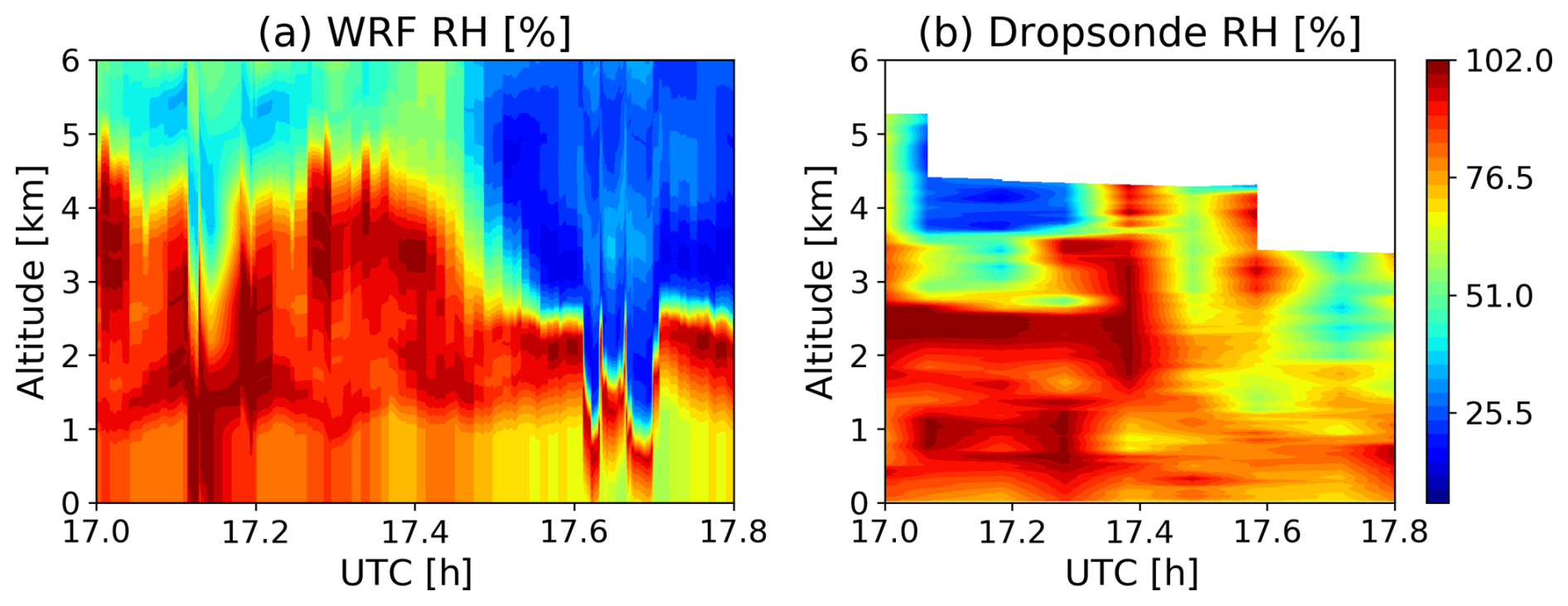
Figure 8 Timeseries of (a) WRF model simulated relative humidity (RH, unit in %) and (b) dropsonde observed ones during the same period of Fig. 7 (17:00–17:48 UTC).

For the last step of the entire closure study, we shall validate the remote sensing retrievals using independent 2D-S cloud probe “observations”. By adding the quotation mark, it is important to stress again that cloud probe “observations” are also “retrievals” with orders of magnitude difference in scales. As mentioned previously, P-3 co-flew with ER-2 only during 16:12–17:30 UTC. Hence we can identify 2D-S retrievals from collocated radar range bins where P-3 was cruising as collocated and coincident in-situ IWC “truths”. It turns out these collocated samples cover more than 3 orders of magnitude of IWC values, and the radar retrievals turns out to agree quite well for all values with a slight over-estimation for IWC<0.1 g m⁻² (Fig. 9). Note that the Brown and Francis (1995) m–D relationship is assumed here to convert 2D-S images to IWC retrievals. If other m–D relationships are used, as will be shown later in Sect. 3.3, they will alter the bias direction. We shall hence focus on the excellent overall agreements, which nicely concludes this closure study.

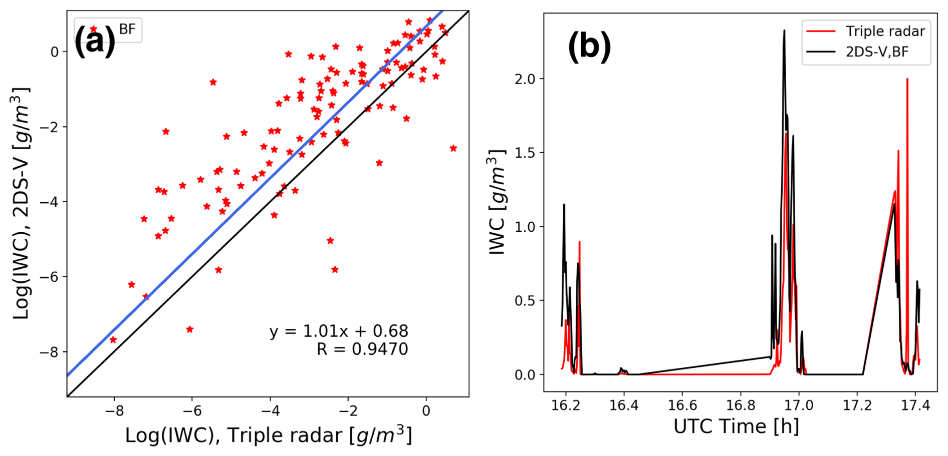
Figure 9 Comparison between joint CRS+HIWRAP IWC retrievals and 2D-S cloud probe retrievals at the collocated radar range bin where P-3 was cruising. (a) Scatter plots from the collocated samples and (b) displaying the same data samples using a timeseries. The Brown and Francis (1995) m–D relationship is used for 2D-S. Linear regression results for (a) are added as the blue line and equation/R-value written in the bottom right corner of panel (a).

3.2 CoSSIR-only prediction of vertical profiles of hydrometeor type

This section will explore the advantage of polarimetric difference ($\text{PD}\equiv {\text{TB}}_{\text{V}}-{\text{TB}}_{\text{H}}$) in helping differentiating the hydrometeor type both vertically and horizontally. Although CoSSIR is a passive sensor that collects the WF-weighted vertically-integrated information, the fact that different channel WFs give preference at different altitudes suggests that CoSSIR has capabilities, although likely limited, at differentiating vertical profiles of hydrometeors. This is also vividly suggested in Figs. 7 and 10.

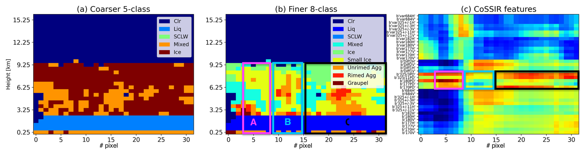
Figure 10 Combined (a) 5-class and (b) 8-class hydrometeor classifications for a cross-section of the storm, and (c) the collocated and coincident CoSSIR measurements (normalized for each variable). From bottom to top in (c): radiance (TB) following the order listed in Table 1 with V-pol first followed by H-pol for each frequency, polarization difference (PD) for 170, 177, 180, 325±11, 325±3.4 GHz, TB difference between different channels (325±11 V–170 V, 325±11 H–170 H, 325±3 V–180 V, 325±3 H–180 H) and variance of 14 channel TBs. All values have been normalized using min-max method with values ranging from 0 (deep blue) to 1 (bright red). The three colored rectangles encircle three different vertical cloud structures and their corresponding PD signals in CoSSIR. The PD signals are measured at 170, 177, 180, 325±11 and 325±3 GHz from lower to upper rows. Note that the horizontal resolution of (a) and (b) are coarsened both horizontally to ∼500 m to match CoSSIR footprint size, and vertically to ∼250 m. See text for the discussion about Regime A, B, and C circled in (b) and (c).

Figure 10a and b showcase an example of triple-frequency radar retrieved hydrometeor types (a for 5-class, and b for finer 8-class categorization) for a contiguous 32-footprints (∼32 km) nadir-looking curtain. The originally 240 m vertical resolution is coarsened to 500 m, partially because the image size (16 km × 32 km $=\mathrm{32}\times \mathrm{32}$ pixels) is more suitable for machine learning (ML) training, and more importantly, due to the concern that CoSSIR is at its best able to tell apart 7-layers of vertical information indepedently according to our previous information content analysis (Liu et al., 2026). This translates into about 1 km vertical resolution for a 7 km thick ice clouds, or 500 m vertical resolution for a shallow 3 km thick ice clouds. In practice, the actual vertical resolution is about 2 km in most scenarios (Liu et al., 2026), so we should bear in mind that our ML exercise here tends to be on the optimistic side. Figure 10c stacks from bottom to top normalized CoSSIR observed TB, PD and ${\mathit{\sigma }}_{\text{TB}}^{\mathrm{2}}$ along the horizontal axis for the 32 observations, where rich information can be clearly seen from the polarimetric measurements (i.e., rectangle enclosed regions). The pink, light blue and black rectangles in Fig. 10 highlight three regions where the vertical cloud structures are distinctively different, namely anvil clouds (A), middle-layer ice core (B) and stratiform precipitating layers (C). This is the first time that PDs are compared amongst different channels laterally for a weather system, where we see greater channel-by-channel variations compared to the constrasts among TBs measurements from different channels. Typically speaking, for the same channel frequency, a larger PD accompanied by cold TB usually suggests dominantly horizontally oriented large ice particles (e.g., rosette), a smaller PD with warm TB indicates small cloud ice with no preferred orientation, but a smaller PD with cold TB implies possible turbulence inside convective cores (Gong and Wu, 2017; Gong et al., 2020). Combining PD and TB from different channels therefore unveils more details. For example, PD at 180 and 325.15±3 GHz both enhance significantly in Zone A. Because both of these channels are close to the water vapor absorption line, their enhancements indicate a significant anvil layer dominated by horizontally oriented ice. Meanwhile, as TB across all CoSSIR bands remain the coldest among this scene for Zone A with PD enhancement at 170 GHz, we can infer a large IWC layer in the lower troposphere with small vertical velocity, i.e., a dying convective core. This is also clearly indicated in the radar hydrometeor classification figure by the heavily riming aggregates and graupel near 3.25 km in Zone A. As a contrast, 325±11 GHz with WF peaking at around 6–7 km, shows a PD enhancement in Zone C, which indicates an alofted stratiform layer at 6–7 km. In Zone B, TBs are relatively warm, PDs are small, which could correspond to a shallow congestus or developing shallow convection with fresh unrimed ice and larger internal vertical velocity.

The ML segmentation task employs the full set of CoSSIR channel TB, PD and ${\mathit{\sigma }}_{\text{TB}}^{\mathrm{2}}$ observations except 182.3 V and 325±0.9 V as we experienced some calibration issues with these two bands and data quality was not satisfying (data quality backed to normal after 31 January for these two channels). This yields a total of 36 input features and the target is 9-class hydrometeor type (clear-sky is included as the 9th class) at 500 m vertical resolution between 0–16 km. The radar curtain is randomly cropped into images with 32×32 pixels in size as the example shown in Fig. 10b. To avoid data leaking, we employed a total of 1575 training images from the 5 February 2023 winter storm case, and target at predicting 479 independent testing samples from this 15 January 2023 case. In the 1575 training samples, training/validation was split at 80 % $/$ 20 % ratio. A standard fully-connected Unet segmentation model is employed in this ML task with 5-layer model depth and a standard binary cross entropy (BCE) loss function. Since this paper is by no means intended as a ML-oriented effort, we didn't a run a full grid search of optimal hyperparameters. Rather, with a satisfactory performance after several trials, we apply exactly the same set of hyperparameter values and identical model to another sensitivity test that excludes all 6-channel PDs. The baseline model is called “full-set”, and the sensitivity test is called “No-PD”. Although BCE loss function was employed for training and testing, the mIoU (Mean Intersection over Union) score is also used as the evaluation metric. mIoU is defined as:

$$\begin{array}{}\text{(2)}& \text{mIoU}\equiv {\displaystyle \frac{\mathrm{1}}{\mathrm{9}}}{\mathrm{\Sigma }}_{i=\mathrm{1}}^{\mathrm{9}}{\displaystyle \frac{{\text{TP}}_i}{{\text{TP}}_i+{\text{FP}}_i+{\text{FN}}_i}}\end{array}$$

where TP, FP and FN stand for true positive, false positive and false negative, respectively. mIoU score ranges from 0 to 1, where 0 means every pixel is segmented into a wrong class while 1 means every pixel is segmented correctly (i.e., a perfect match between predicted image and reference truth). Typically a mIoU score of 0.5 is considered a good result for 9-class segmentation tasks, and a value of 0.7 or higher usually indicates a very high-quality result.

The mIoU score for the baseline full-set model and no-PD sensitivity run is 0.642 and 0.4024, respectively. Both of the scores indicate descent retrieval potential of CoSSIR in distinguishing vertical hydrometeor structures. Figures 11 and 12 give two example scenes, one for the deep convective cloud with three cloud layers at the outskirt, and the other with boundary layer broken mixed-phase clouds and liquid precipitation layer beneath. For the former complicated multi-layer thick cloud scene, we can see excluding PDs is really limited in reproducing the true vertical cloud structure (Fig. 11a vs. b), although it does reasonably well in capturing the location of convective core, the rough vertical separations of frozen and liquid hydrometeors and the overall geometric thickness. Once PD measurements are included, the prediction quality improves dramatically. When the cloud layer is thin and low, both ML models perform relatively poorly, but including PDs help in general. For example, both ML models predict a wrong cirrus cloud layer in the upper troposphere for the multi-layer boundary layer cloud scene shown in Fig. 12, including PDs seems to be not critical, although the no-PD prediction gives a false cirrus cloud for this case (not for many other similar scenes). Yet, including PDs effectively predict the mixed-phase layer above the liquid layer correctly while the No-PD model missed in predicting the existence of the mixed-phase layer completely.

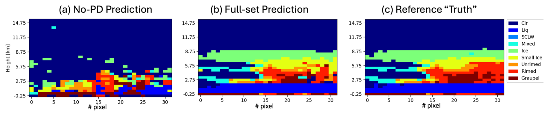
Figure 11 Prediction without (a) and with (b) using PDs and reference truth (c) of a deep convective clouds with multi-layer features.

Figure 12 Same with Fig. 11, except for a double-layer boundary layer cloud scene.

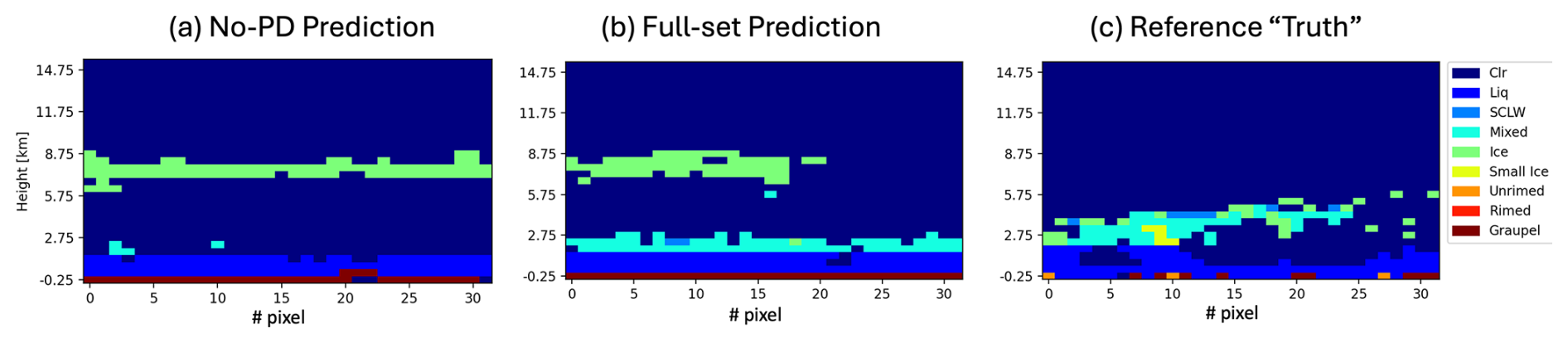
The limitation of No-PD retrieval of hydrometeor vertical type for thick ice cloud is as expected because TBs at >183 GHz lacks the channel-by-channel contrast when encountering thick ice cloud layers. This is also suggested by Fig. 10c and the example channel response function (CRF) shown by Fig. A2 in the Appendix. Although our current RT capabilities limit us in simulating the correct response function for PDs for thick clouds, the ML experiments clearly demonstrate the merits and potential. For single-layer thin ice clouds, there are enough differentiations among 183.31, 325.15 and 684 GHz wing bands to unveil vertical variations. As for boundary layer warm clouds, CoSSIR lacks the lower-frequency bands that are sensitive to liquid emissions. Yet, Fig. 12 and many other lower cloud scenes (not shown) demonstrate that PD signals might be very useful in telling apart liquid from mixed-phase clouds in the boundary layer.

Lastly, it is worth emphasizing that we intentionally designed to train on a typical winter storm case (5 February) and to predict on an atypical case (15 January) to test the robustness of our hypothesis that CoSSIR PD signals contain useful information about the vertical hydrometeor phase distribution. As most of the IMPACTS cases are typical winter storm cases, making a good prediction on another winter storm case might be partially explained by the similarity of winter storm vertical structures.

3.3 CoSSIR single-channel D_me retrieval

In this last objective, we further explore the merit of using PD in constraining the ice particle habit and size. Gong and Wu (2017) found a statistically robust upside down “bell-curve” for the PD–TB relationship using the Global Precipitation Measurement Microwave Imager (GPM-GMI) observations at 166 GHz. They also identified a similar curve for 684 GHz using CoSSIR observations collected during the TC4 campaign over deep tropics. They further found the value range of PD is strongly dependent on the ice particle shape assumption, while the curvature of the bell curve is a function of mass-weighted ice particle diameter (D_me). Wu et al. (2024) further proposed a look-up-table (LUT) method to retrieve D_me using a single frequency PD–TB measurements. All these conclusions were based on highly idealized RT simulations assuming 100 % horizontal orientation, one single ice habit in the entire column, and a box cloud shape with fixed cloud top and bottom height. Whether such a LUT approach can work in real world cases was never explored.

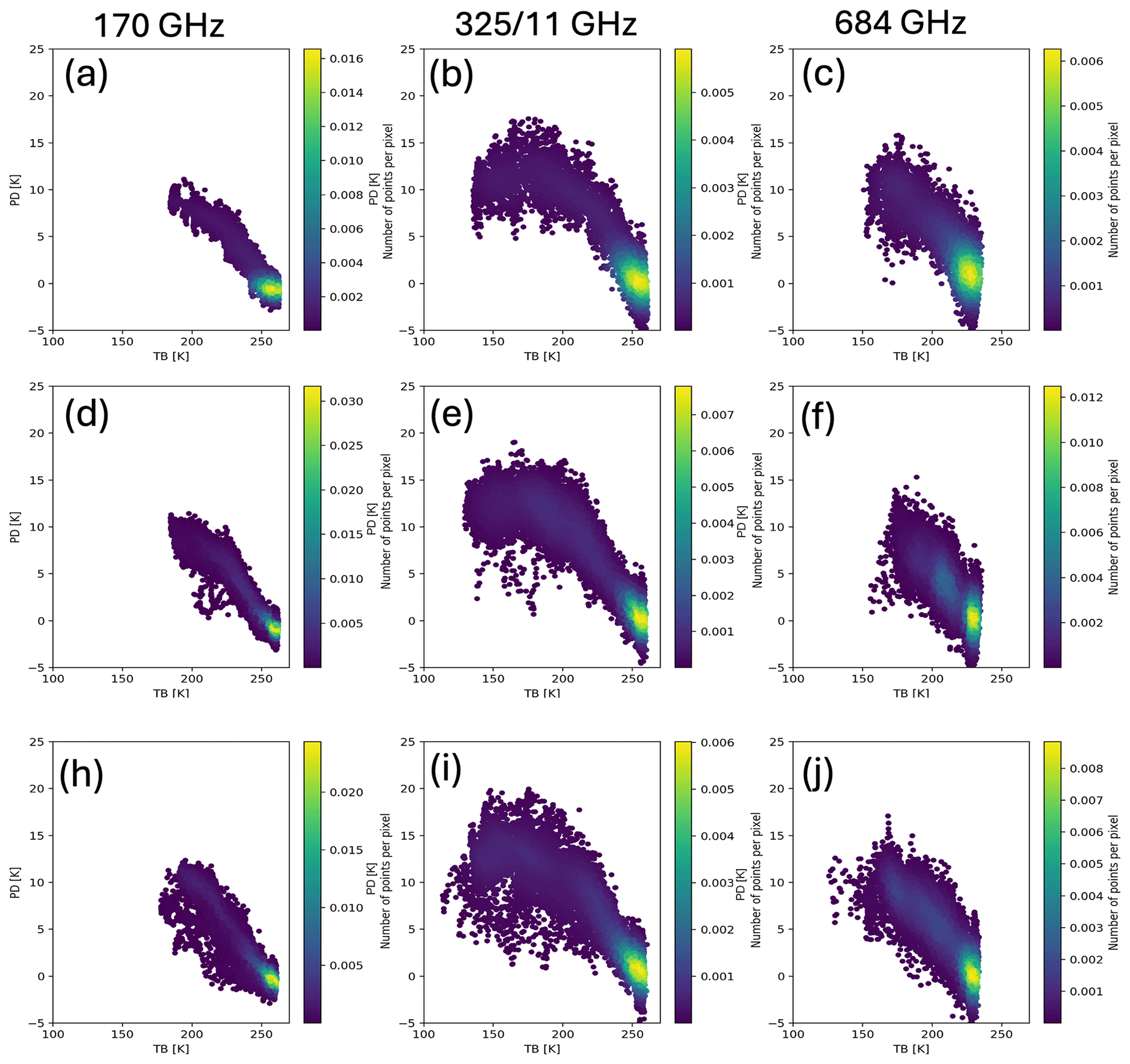
In this vein, we first inspected the PD–TB scatter plots from three different channels, presumably with WF peaking at different altitudes. The entire period of interest is also separated into three sub-periods: 16:05–16:24, 16:48–17:03 and 17:15–17:30 UTC to exclude contamination of the general statistics from clear-sky or pure-liquid scenes because the LUT method does not apply to these scenes. Such a segmentation also originates from the consideration to separate samples from different stages because the microphysical properties could evolve. The statistical relationship from the first sub-period is shown in Fig. 13, while all three sub-periods are displayed in Fig. B1.

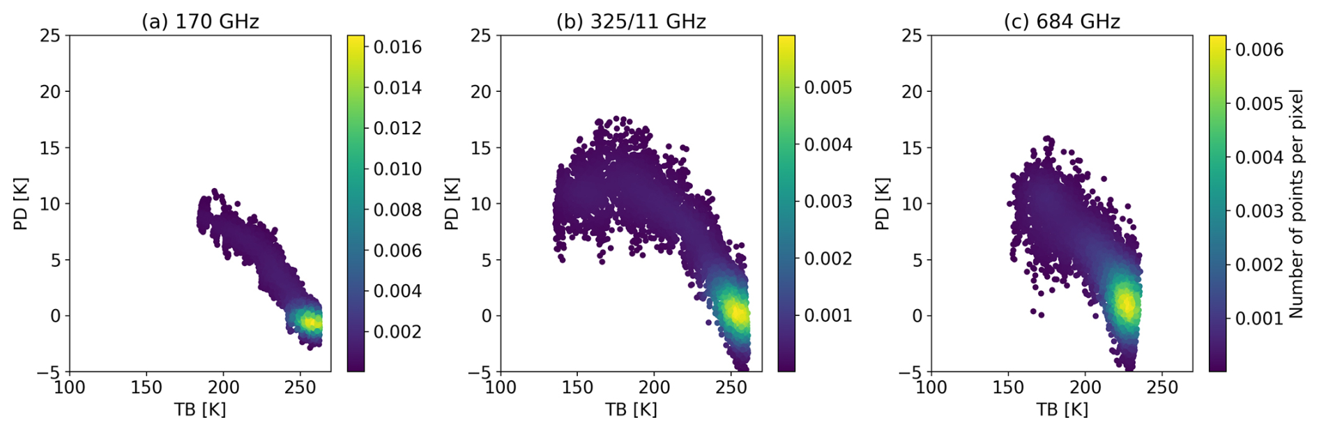
Figure 13 Density plots of the observed PD–TB relationship during 16:05–16:24 UTC for (a) 170, (b) 325.15±11 and (c) 684 GHz.

Firstly, the upside down bell-curve does not present in 170 and 684 GHz like what was previously discovered using tropical observations. This is because this 15 January warm-core cyclone never introduced cold enough TB nor strong enough turbulence to drive the PD value back to zero at cold TBs. 325.15±11 GHz shows the largest dynamic range of TB for this system, which is as expected and the most suitable for applying the LUT method (see Fig. A2 in the Appendix for a detailed explanation). Secondly, the largest PD value is ∼15 K, which indicates 6-bullet rosette is likely the most proper ice habit assumption as other particle shapes we tried (plate, column, dendrite) all produce too large PD (40–80 K). Two examples are given in Fig. 14. As a matter of fact, 6-bullet rosette assumption holds as the best choice for all three sub-periods. Lastly, we apply the LUT method to CoSSIR 325.15±11 GHz as its WF peaking height is the closest to P-3 cruising altitude during this period. The retrieved D_me can then be compared against collocated 2D-S retrieved ones.

Figure 14 Look-up-table (LUT) for 325.15+10 GHz for (a) 6-bullet rosette and (b) column ice.

The comparison results are shown in Fig. 15. Three different m–D relationship assumptions are employed to generate D_me retrievals from 2D-S, and we can see the single-channel retrieval results match well to the reference no matter what m–D relationship is chosen, although Brown and Francis (1995) seems to produce the best matches in this case. Further, we can clearly observe an increase of ice particle size along with time, which agree with our previous observation of the evolvement of hydrometeor vertical structures over time (Fig. 5).

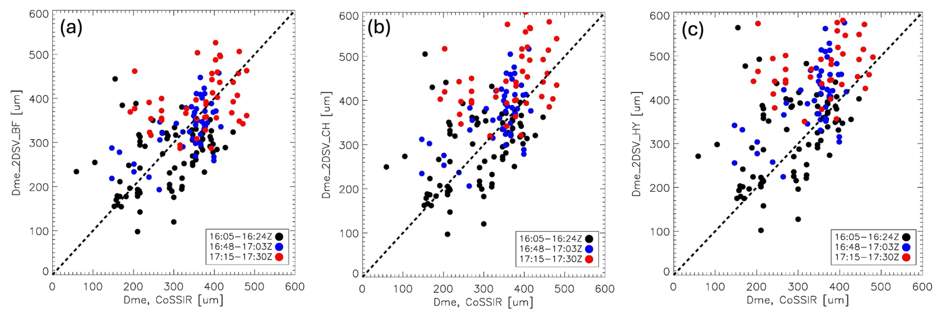
Figure 15 Scatter plots of retrieved D_me from CoSSIR 325.15±11 GHz (horizontal axis) in comparison with collocated 2D-S retrievals using the m–D relationship from (a) Brown and Francis (1995), (b) Chase et al. (2021) and (c) Heymsfield et al. (2010). Black, blue and red dots are taken from 16:05–16:24, 16:48–17:03 and 17:15–17:30 UTC periods, respectively.

4 Discussion

Although we have discussed many details in the results section, including caveats in the data or current approach, we still want to dedicate this section to discuss cross-latitude comparison against similar works, as well as some known caveats that can be improved in the future.

First, closure study is the focus of this paper, which was inspired by McCusker et al. (2024). Findings from both papers stress the criticality of having more detailed vertical profiles of hydrometeor phase and habits to reach agreement among in-situ, active and passive remote sensing measurements. Albeit, our research took a distinctively different approach compared to McCusker et al. (2024), mainly because of more data availability from different instruments and the co-flying design with two aircrafts (Yorks et al., 2025). As the case in McCusker et al. (2024) installed the cloud probe on the same aircraft with European's sub-mm airborne instrument ISMAR, the airplane flew back and forth through the same winter frontal system while gradually descending its altitude so to sample the full cloud system from remote sensing measurements using the first half segment and sample the in-situ “truth” using cloud probes during the second half of the flight leg. Due to the temporal mismatch between remote sensing and in-situ measurements, the authors had to assume ice particle habit remaining unchanged throughout, which also means that they had to miss the opportunity of studying microphysics evolution like what we can do here in Fig. 15. Their flight leg design, however, provided vertical profiling of ice habit and size, which our flight trajectory design was not able to capture. In addition, the Ka-band radar was installed on a different aircraft, and the two flights were not coordinated to fly together in their case. This fact obviously adds challenges to the McCusker et al. (2024) case analysis, because they not only needed to assume the frontal system did not change between two aircraft overpasses, but also lacked detailed vertical information about hydrometeor microphysics by using Ka-band radar reflectivity measurement only for generating input hydrometeor profiles for forward simulations for ISMAR channels. The co-flying pattern between two aircrafts during the IMPACTS campaign is examplatary to future airborne campaign design to boost science discoveries.

Second, for the ML-based hydrometeor type profile retrieval, the intention is to highlight the advantage of polarimetric measurements instead of delivering a mature algorithm/product. Rather, our companion paper (Liu et al., 2026) provides a much more strict retrieval algorithm for hydrometeor profiling with a thorough information content analysis. Note that while Liu et al. (2026) builds its algorithm upon the heritage Bayesian theorem-based retrievals, it assumes one ice habit at a time for the whole column to retrieve the vertical mass distribution, while this work focuses on exploring potential research product enabled by additional polarimetric measurements. Interested readers are recommended to explore that paper as well as May and Eriksson (2025). We anticipate to explore further a combination of ML and Bayesian frameworks to advance the retrieval algorithm development of hydrometeor profiles in the future.

Last but not the least, the single-channel size retrieval using PD and TB is the first observational proof-of-concept of the previously proposed approach using idealized RTM simulations. Although the results are indeed very encouraging, a few assumptions need to be postulated to simplify the LUT table computation. One of the assumption is same particle habit in the column, which is likely not the case in real world. In addition, once deviating from scan-angle 52.8°, the degree of randomness (i.e., percentage of particles that are horizontally oriented) starts to matter more and more, so the application of this PD–TB single band retrieval method will face challenges for cross-track scanners. Nevertheless, we believe this pilot study points to a viable direction that could make PD operationally usable for retrieving ice microphysics or at least becoming part of the operational algorithm to constrain the retrieval errors.

5 Conclusions

To summarize, this paper paves some concrete steps in assuring timely delivery of high-quality science products for the sub-mm radiometer missions as well as possibilities of new science products beyond the mission requirements. This current research explores three inter-linked objectives: an in-situ, active and passive remote sensing closure study to emphasize the criticality of having the correct vertical profiles of hydrometeor type, and two research objectives to explore the scientific merits of sub-mm polarimetric measurements in (1) facilitating the hydrometeor profiling; and (2) constraining the frozen hydrometeor particle size. This entire work is built upon a carefully designed and successfully executed airborne campaign that enables myrid ways leading to new scientific discoveries.

The closure study is designed as an extension of regular satellite algorithm validation effort. Through this work, we would like to emphasize that active remote sensing measurements, although usually treated as the “truths” for validating passive satellite measurements or algorithms, need to be carefully “pre-processed”, or otherwise the discrepancies tend to often be interpreted as “biases” from the passive sensor measurements while inconsistent microphysics assumptions across different retrievals are indeed the culprit. Similarly, for “in-situ truth”, which also relies on certain assumptions to “retrieve” the “reference truth”, the drastic measurement scale difference should be factored in in order to make fair and meaningful validations.

Results about the scientific usefulness of PD are preliminary and require extensive studies with more carefully designed strategies in order to make the latter two into reliable research products for upcoming sub-mm satellite missions. To the least extent, we will need to apply the same strategy to more cases over different weather regimes (e.g., cold front, warm front, tropical convective systems, etc.) in order to understand the advantages and limitations. For the PD-based size retrieval, we need to build the LUT approach into the retrieval workflow in order to take advantage of the PD measurements operationally.

Appendix A: Channel response function (CRF) for thick clouds

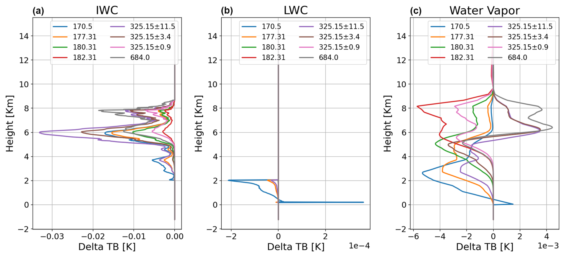
We provide Fig. A1 and its corresponding Jacobians to hydrometeors and water vapor in Fig. A2 to support two purposes in the main text: first, to demonstrate that No-PD loses hydrometeor profiling capabilities when the frozen hydrometeor layer is very thick, because that CRFs to IWC all look very similar in terms of shape (Fig. A2a). Nevertheless, we can still see from the same panel that 170.5, 177.31 and 325.15±11.5 GHz channels are capable to penetrate deep in this case to still capture the bottom layer IWC between 2–4 km. TB signal is dominated by frozen hydrometeors when ice cloud is thick, since the Jacobians to IWC are one order of magnitude larger than that to water vapor (Fig. A2c), and two orders of magnitude larger than that to LWC (Fig. A2b). Secondly, this example is intended to justify why the 325.15±11.5 GHz channel retrieved D_me is used to compare with the 2D-S references, as it is clearly seen that this channel has a the largest WF response to frozen hydrometeors at 5–7 km, the level where 2D-S took most of its measurement between 16:00–18:30 UTC.

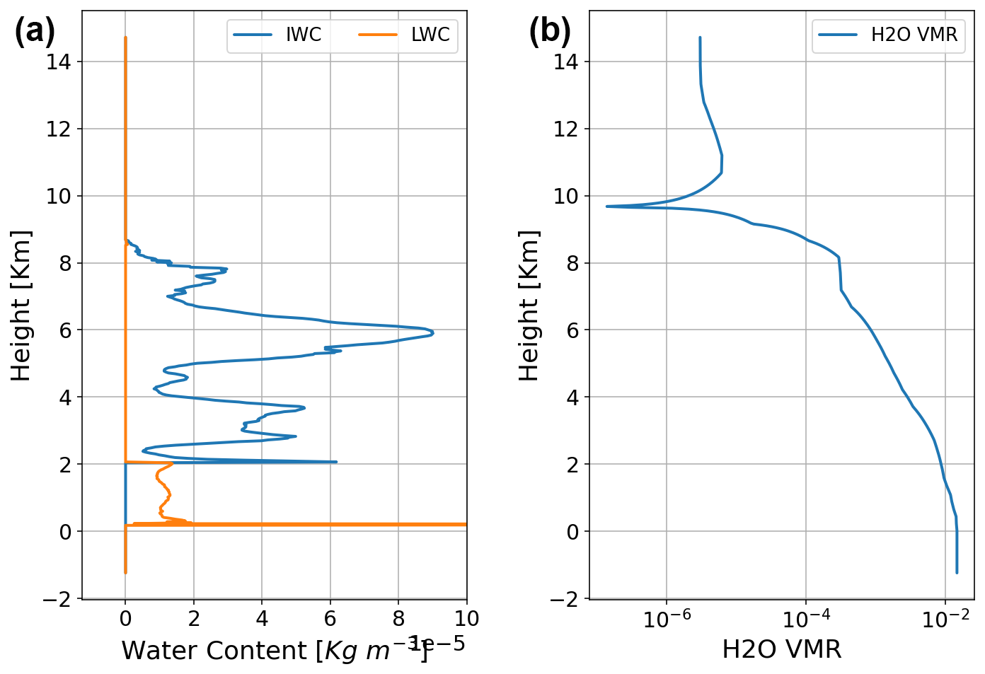
Figure A1 Sample (a) IWC (blue), LWC (orange) and (b) water vapor mixing ratio profiles at 18:00 UTC. IWC and LWC are retrieved from triple-frequency radar measurements, and water vapor mixing ratio is from the WRF simulation.

Figure A2 Jacobians for each channel for (a) IWC, (b) LWC and (c) water vapor that are provided in Fig. A1. The Jacobians are computed by perturbing each layer by 1 % each time. Please note the value range in the horizontal axis.

Appendix B: PD–TB relationship for different sub-period

Figure B1 Same with Fig. 13, except the second row is made up from samples collected during 16:05–16:24 UTC, and last row from 17:15–17:30 UTC.