Fractal characteristics of ice-supersaturated regions in the tropopause region of the northern midlatitudes

Ice supersaturated regions (ISSRs) are air masses in the upper troposphere and lower stratosphere (UTLS) where saturation ratio over ice (S_i) exceeds one, i.e. regions with enhanced water vapor concentrations. These are potential formation regions of cirrus clouds and contrails. While the impact of cloud free regions of enhanced water vapor on the planetary radiation balance is small to negligible, thin cirrus clouds and aircraft induced contrail cirrus formed within them might have a large radiative impact. Understanding the characteristics of ISSRs, including their geometry and seasonal variability, is essential for evaluating atmospheric models in representing ice clouds correctly. While ISSR's pathlength statistics, i.e. 1D characteristics, have already been studied, their geometric properties, particularly fractal properties such as self-similarity, and their seasonal variability remain largely unexplored. We identify ISSRs using ERA5 reanalysis data spanning from 2010 to 2020 at three pressure levels. An area-perimeter method is employed to compute fractal dimensions. The results reveal slopes implying fractal dimensions, strongly suggesting that ISSRs in the UTLS exhibit fractal behavior. A seasonal cycle in total number and area of ISSRs, as well as in the fractal dimension is found, in combination with a strong vertical variation. We hypothesize that this is caused by the seasonal variation of convective and frontal activity. We further analyzed the zonal and meridional extents of ISSRs as well as the pathlengths of modeled flights along commercial flight routes. The results of these horizontal extents are consistent with the fractal properties, and suggest distinct formation processes for ISSRs.

1 Introduction

Ice supersaturated regions (ISSRs) in the upper troposphere and lower stratosphere (UTLS) serve as key environments for the formation and persistence of in situ cirrus clouds. These regions occur when the water vapor partial pressure p_v exceeds the water vapor saturation pressure over ice at temperature T, leading to a saturation ratio

$$\begin{array}{}\text{(1)}& S_{\mathrm{i}}={\displaystyle \frac{p_{\mathrm{v}}}{p_{\mathrm{si}}\left(T\right)}}\end{array}$$

greater than one. Ice supersaturation (first described by Alfred Wegener, 1910, 1911) is a frequent and widespread phenomenon in the UTLS (Gierens and Spichtinger, 2000; Spichtinger et al., 2003b; Gettelman et al., 2006; Lamquin et al., 2012; Petzold et al., 2020; Reutter et al., 2020), where the cold and dry conditions render even small variations in humidity highly significant. ISSRs not only serve as a key environment for the formation of in situ cirrus clouds (Krämer et al., 2016), but also as a prerequisite for persistent contrails (Schumann, 1996; Stuber et al., 2006; Lee et al., 2010, 2021; Petzold et al., 2025). Currently, this is a major topic in the context of contrail avoidance, since contrails can persist for over 10 h and spread into contrail cirrus (Haywood et al., 2009). Cloud free ISSRs have a relatively minor direct influence on the local radiation budget, but their transition into cirrus clouds significantly alters radiative forcing (Fusina et al., 2007). ISSRs and cirrus clouds are predominantly found in the upper troposphere, but they can also extend above the tropopause (Spichtinger et al., 2003a; Reutter et al., 2020), affecting the lower stratosphere (LS). The upper troposphere–lower stratosphere (UTLS) region is characterized by extremely cold and dry air masses (Dessler and Sherwood, 2009; Held and Soden, 2000). Outgoing longwave radiation is particularly sensitive to small relative perturbations in UTLS water vapor (Clough et al., 1992). Gradients in saturation ratio are closely related to the respective changes in longwave radiation (e.g. Fusina et al., 2007), potentially resulting into local changes of the thermodynamic structure of the tropopause region (Köhler et al., 2024). Consequently, variations in ISSR occurrence and cirrus cloud formation within this region have important implications for climate dynamics and radiative balance (Lee et al., 2010). ISSRs are not necessarily cloud free air masses (Spichtinger et al., 2004), despite former investigations (e.g. Gierens and Spichtinger, 2000) suggesting this property. The transition from ice clouds to cloud free air is very smooth and usually there are no sharp boundaries. In our study we will not further distinguish between clear and cloudy air, as we are interested in the thermodynamic state of the air masses. While studies have examined the horizontal extent of ISSRs using pathlength statistics (Gierens and Spichtinger, 2000; Diao et al., 2014; Spichtinger and Leschner, 2016; Reutter et al., 2020), their two-dimensional spatial characteristics, including shape and scaling behavior, remain poorly understood and have not been studied in detail yet. Statistical investigations are challenging because of the ISSRs' variability in size and shape. In addition, some metrics must be defined (or even developed) for studying ISSRs as 2D/3D objects, instead of just using point measurements. The radiative effects of cirrus clouds, related to either natural or anthropogenic origins, are a subject of ongoing research. This study emphasizes the structural and statistical properties of ISSRs. Understanding their morphology and variability is essential for improving microphysical parameterizations and interpreting the atmospheric processes that control cloud evolution in the UTLS.

A potential approach in studying the geometric properties of 2D or 3D objects is to examine their potential self-similarity, i.e. the fractal properties of these macroscopic objects. In general, fractals are geometric structures characterized by self-similarity. These objects exhibit similar patterns on different scales. They differ from traditional Euclidean shapes by possessing non-integer (fractional) dimensions that describe the way their complexity changes with scale (Peitgen et al., 2004). The research field of fractal geometry was defined by Mandelbrot in 1975, and became prominent in the 1980s (e.g., Mandelbrot, 1982). Investigations on the fractal nature of natural objects were made before Mandelbrot. Notably, Richardson (1926) carried out first investigations on the nature of turbulence, already addressing fractal properties. Thus, fractal analysis has a longstanding tradition in atmospheric physics, especially in cloud physics. In numerous previous studies, the fractal nature of clouds is investigated, ranging from cumulus cloud statistics and properties (Cahalan and Joseph, 1989; Joseph and Cahalan, 1990; Cahalan et al., 1994; Gotoh and Fujii, 1998; Siebesma and Jonker, 2000), rain and hail clouds (Lovejoy, 1982; Lovejoy and Mandelbrot, 1985; Rys and Waldvogel, 1986), tropical clouds (Benner and Curry, 1998; Batista-Tomás et al., 2016), noctilucent clouds (von Savigny et al., 2011; Brinkhoff et al., 2015), and cloud fields in high resolution models (Christensen and Driver, 2021). Additionally, fractal analysis is a key technique for turbulence theories and data evaluation (e.g., Sreenivasan and Meneveau, 1986; Sreenivasan, 1991). In some studies, clouds and turbulence investigations are combined in order to explain fractal properties of clouds by the underlying turbulence (or diffusion) characteristics (e.g., DeWitt et al., 2024; Rees et al., 2024). Overall, there is strong evidence that clouds at different vertical levels show fractal behavior. Thus, it is reasonable to question whether their potential formation regions, i.e. the ISSRs for ice clouds, exhibit similar properties. If this holds true and ISSRs also display self-similar characteristics, determining their fractal dimension can provide insight into their spatial attributes and characteristics.

To identify and study ISSRs, we analyze ERA5 reanalysis data that incorporates absolute humidity, temperature and pressure. Working with a simplified binary representation of ISSRs, connected areas are identified and their areas and perimeters are calculated. To assess the fractal characteristics, especially the self-similarity of ISSRs, we examine the area-perimeter relation. This relation and variations of it have been used in many investigations of clouds (Lovejoy, 1982; Lovejoy and Mandelbrot, 1985; von Savigny et al., 2011; Vogelaar and Wakker, 1994; Batista-Tomás et al., 2016). Such an analysis provides a quantitative measure of the macroscopic structures and has important implications for further investigations.

The study is structured as follows: In Sect. 2 the data set and the methods are introduced. In Sect. 3 the fractal characteristics of ISSRs as found in the data are investigated. This is followed in Sect. 4 by the investigation on the horizontal extent of ISSRs. The results are discussed and conclusions are drawn in Sect. 5. Additional results are presented in the Supplement.

2 Data and Methods

In this section we present the data set and describe the methods used for the investigation of the data.

ISSRs are naturally occurring physical phenomena whose boundaries are inherently gradual rather than sharply defined. Their identification using gridded reanalysis fields necessarily imposes discrete representations of these continuous structures. Although these representations are not identical to the physical structures in nature, they provide a consistent basis for quantifying the geometry and occurrence of physically meaningful supersaturated regions.

2.1 Data set ERA5

The study analyzes eleven years of ERA5 reanalysis data (Hersbach et al., 2020) covering the period from 1 January 2010, to 31 December 2020. Data is available at the standard synoptic times each day (00:00, 06:00, 12:00, 18:00 UTC), resulting in a total of 16 060 datasets for analysis. ERA5 provides data with a horizontal resolution of 0.25° in longitude and latitude, and a vertical resolution of 137 model levels with an approximate resolution in the tropopause region of about 300 m. The data set contains variables of 3D winds ($u,v,w$), temperature T, and specific humidity q. For the investigation we distinguish water vapor in air masses in the state of sub or super saturation with respect to ice. The geographical area used for the analysis is narrowed down to range from 80 to 30° latitude in the Northern Hemisphere in order to exclude the tropics and polar regions. In our investigation we focus on pressure levels of 200, 250, and 300 hPa, representing the upper troposphere and tropopause region (similarly to the investigation by Lamquin et al., 2012). The data on adjacent model levels were interpolated on the respective isobaric surfaces.

2.2 Methods

Here, we briefly describe the processing of the data; for details we refer to Appendix A.

2.2.1 Relevant variable

The thermodynamic order parameter for ISSRs is the saturation ratio

$$\begin{array}{}\text{(2)}& S_{\mathrm{i}}={\displaystyle \frac{p\cdot q}{\mathit{ϵ}\cdot p_{\mathrm{si}}\left(T\right)}}={\displaystyle \frac{p_{\mathrm{v}}}{p_{\mathrm{si}}\left(T\right)}}\end{array}$$

as calculated from the ERA5 variables p, T, q, using the ratio of molar masses of water and air, i.e. $\mathit{ϵ}=\frac{M_{\mathrm{v}}}{M_{\mathrm{d}}}$ and the saturation vapour pressure over (hexagonal) ice p_si in the formulation by Murphy and Koop (2005), i.e.,

$$\begin{array}{}\text{(3)}& \begin{array}{rl}{p}_{\mathrm{si}}& =\exp (\mathrm{9.5504}-{\displaystyle \frac{\mathrm{5723.265}}{T}}+\mathrm{3.53068}\log (T)\\ & -\mathrm{0.00728332}T),\end{array}\end{array}$$

Here, T is given in Kelvin and p_si is obtained in Pascal. The formulation is valid for temperatures T>100 K. The thermodynamic equilibrium between vapor and ice is given by S_i=1.

ERA5 data underestimates the humidity in the UTLS region (Köhler et al., 2024). We counteract this by choosing a threshold value of $S_{\mathrm{i},\mathrm{threshold}}=\mathrm{0.9}$. Note that we use no further information about possible clouds inside the ISSRs. A data point is assigned to be supersaturated (i.e.  belonging to an ISSR) if $S_{\mathrm{i}}\ge S_{\mathrm{i},\mathrm{threshold}}=\mathrm{0.9}$. Using this criterion we create a two dimensional binary field with subsaturated data points (index = 0) and data points inside an ISSR (index = 1) for each pressure level. For a macroscopic object we have to specify a measure for the connectivity of single data points (with index = 1) on the gridded isobaric surface. We choose the 8-neighborhood (or Moore neighborhood), i.e. a central pixel is connected to the neighboring pixels via the edges and the diagonals. This definition, originating from investigations with cellular automaton (Chopard and Droz, 1998), is essential, since the connectivity of a physical object should not (or as little as possible) depend on the orientation of a grid. A visualization of different neighborhoods is represented in Appendix A. For a substantial analysis, we consider only ISSRs consisting of at least N=24 pixels, i.e. exceeding a minimum size. Otherwise, a possible self-similar structure would not be reliably resolved. Here, we follow the recommendation of Christensen and Driver (2021). Furthermore, we focus on the midlatitudes in the Northern Hemisphere (30–80° N). As ISSRs may extend into polar or tropical regions, we exclude those objects crossing the boundaries of 30 and 80° N completely (setting the index = 0) to avoid artificially smoothing perimeter and cropping area. For the further evaluation, the resulting connected binary islands (i.e. the ISSRs) are numbered.

2.2.2 Measuring Island Area and Perimeter

The ISSRs are located on the geographical grid of the Earth. Since we use a latitude-longitude description we have to take into account the distortion caused by the curvature of the Earth. Each grid point can be seen as the center of an almost quadratic pixel with a respective area (in square meters, see Appendix A), which can be assigned by using the Python package pyproj.Geod (Snow et al., 2025). For the calculation of the perimeter, we had to develop an additional tool, taking into account the length of the respective boundaries of the pixel without a neighboring pixel. The overall perimeter of the labeled island is calculated iteratively; here, we can determine both internal and external borders.

2.2.3 Calculation of the Fractal Dimension

A key characteristic of fractals is self-similarity, the defining property upon which we base our approach for the dimension of objects. The fractal dimension most commonly refers to the Hausdorff dimension. However, its rigorous determination lies beyond the scope of this work. As the general concept involves progressively increasing the spatial resolution of the data (Peitgen et al., 2004), this procedure is not feasible for real-world data due to the finite resolution. Specifically, gridded data sets such as ERA5 are incompatible with this method, as the resolution is fixed and cannot be refined arbitrarily.

Consequently, a different method must be employed to calculate the dimension for data in two dimensions. For this purpose, the area-perimeter relation is investigated. This type of relationship was introduced by Lovejoy (1982) to study fractal properties of clouds and rain areas, i.e. the self-similarity of such objects. It is defined as a power law relationship between the perimeter P and the area A of a two dimensional object is assumed, such that

$$\begin{array}{}\text{(4)}& P=C\cdot A^{\frac{D}{\mathrm{2}}}⟺\log \left(P\right)=\log \left(C\right)+{\displaystyle \frac{D}{\mathrm{2}}}\log \left(A\right)\end{array}$$

with C a scaling parameter. Using scatter plots of data points (A,P) in a double logarithmic scale, the perimeter shows a linear behavior with respect to the area with a slope α. α is not necessarily an integer number but rather a non-negative real number α∈ℝ. This can be used for calculating the “fractal” dimension $D=\mathrm{2}\cdot \mathit{\alpha }$. For regular geometric objects we obtain a value D=1 (see also the discussion in Appendix B). D should be understood as the dimension of the perimeter. For planar, fractal objects like ISSRs on an isobaric surface we assume $\mathrm{1}<D<\mathrm{2}$. The value of D can be determined by a linear fit with slope α.

As observed by Cheng (1995), the “dimension” D as derived by the area-perimeter relation does not agree with the Hausdorff dimension in general. However, it is appropriate to use this approach in order to study the fractal characteristics and properties of phenomena as shown in other studies (e.g., Mandelbrot et al., 1984; Sakellariou et al., 1991; Klinkenberg, 1994; Florio et al., 2019, for details see Supplement).

For the ERA5 data in this study (as for all gridded data), the perimeter cannot approach infinity as the horizontal resolution limits the frayed nature of the ISSRs' perimeter, further justifying the employment of the area-perimeter method. The dimension calculated with the area-perimeter method will hereafter be referred to as the fractal dimension. As ISSRs have irregular boundaries, the dimension is expected to be in the range $\mathrm{1}<D<\mathrm{2}$. In Appendix B we exemplarily show how the fractal dimension might change by either changing the shape of rectangulars systematically or fraying the boundary of squares.

For gridded data, area and perimeter can only be approximated. Possible errors are underestimation of the area and overestimation of the perimeter, as discussed in Sanchez et al. (2005) and Imre (2006). In Appendix C we investigate these issues for spheres. The analysis indicates that the quality of the evaluation is not compromised. The derived fractal dimensions (i.e. exponents in Eq. 4) can therefore be regarded as robust estimates and are suitable for further, including quantitative, analysis.

3 Fractal properties of ISSRs

In this section we investigate the properties of ISSRs, such as the number and area of ISSRs, and the derived fractal dimension D. Subsequently, their seasonal and annual evolution are investigated.

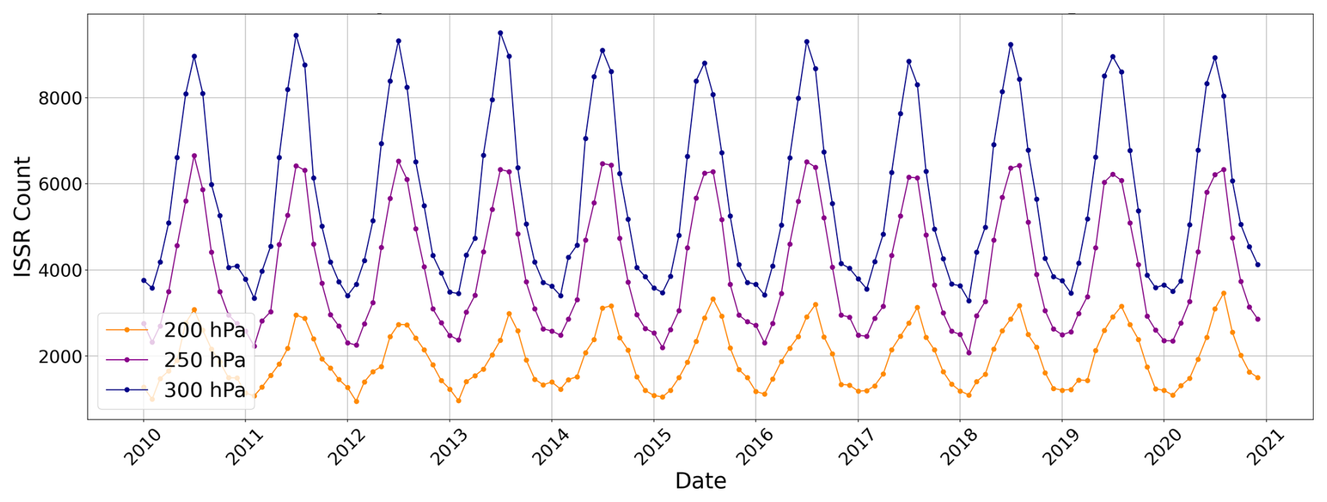
Figure 1 Monthly ISSR Number count from 2010 to 2020 at pressure levels 200 hPa (orange), 250 hPa (violet) and 300 hPa (dark blue).

3.1 ISSR Number Count and Area

Figure 1 shows the number of observed ISSRs by month on the 200, 250 and 300 hPa pressure levels during the period from 2010 to 2020. The total number is a sum of all ISSRs appearing at each point in time. This causes the number to be significantly higher than the ISSRs that appeared in a given month, as ISSRs are counted multiple times when having a life-span longer than 6 h. A clear dependence of the number of ISSRs with altitude is evident. At lower altitudes (i.e. higher pressures) we find significantly more ISSRs than at higher altitudes. This can be explained by the fact that in the extratropics the (thermal) tropopause is located in the pressure range between 300 and 200 hPa, and ISSRs are almost exclusively located in the troposphere. Only few ISSRs seem to reach into the stratosphere (Spichtinger et al., 2003a). Generally, ISSRs are most frequently located close to the tropopause.

The tropopause also shows a seasonal cycle with high altitudes during summer and lower altitudes during winter (e.g., Spichtinger et al., 2003a). Nevertheless, the probability to measure dry and warm air in the stratosphere at a certain pressure level in the extratropics is much higher for pressure level p=200 hPa, than for p=250 hPa or p=300 hPa. This might explain the strong differences in the amount of ISSRs between the three pressure levels. The strong seasonal cycle in the number of ISSRs is a prominent feature, which is most pronounced at pressure level p=300 hPa, i.e. in the upper troposphere. We find maxima in summer and minima in winter for all 3 pressure levels. The month with the highest observed number at pressure level p=300 hPa is July 2013 with 9511 detected ISSRs, the minimum number of 3290 ISSRs at the same pressure level can be observed in February 2018. Respectively, the highest number of ISSRs at pressure level p=200 hPa was recorded in July 2020 with 3462 ISSRs, whereas the minimum was observed in February 2012 with 954 ISSRs. Here, we see the substantial spread in the amount of ISSRs.

The seasonal cycle compares well with former investigations. Spichtinger and Leschner (2016) also found this signature with highest values of ISSR numbers during summer and lowest counts in the winter's season. Furthermore, the strong variation of numbers with the vertical levels agrees well with our findings.

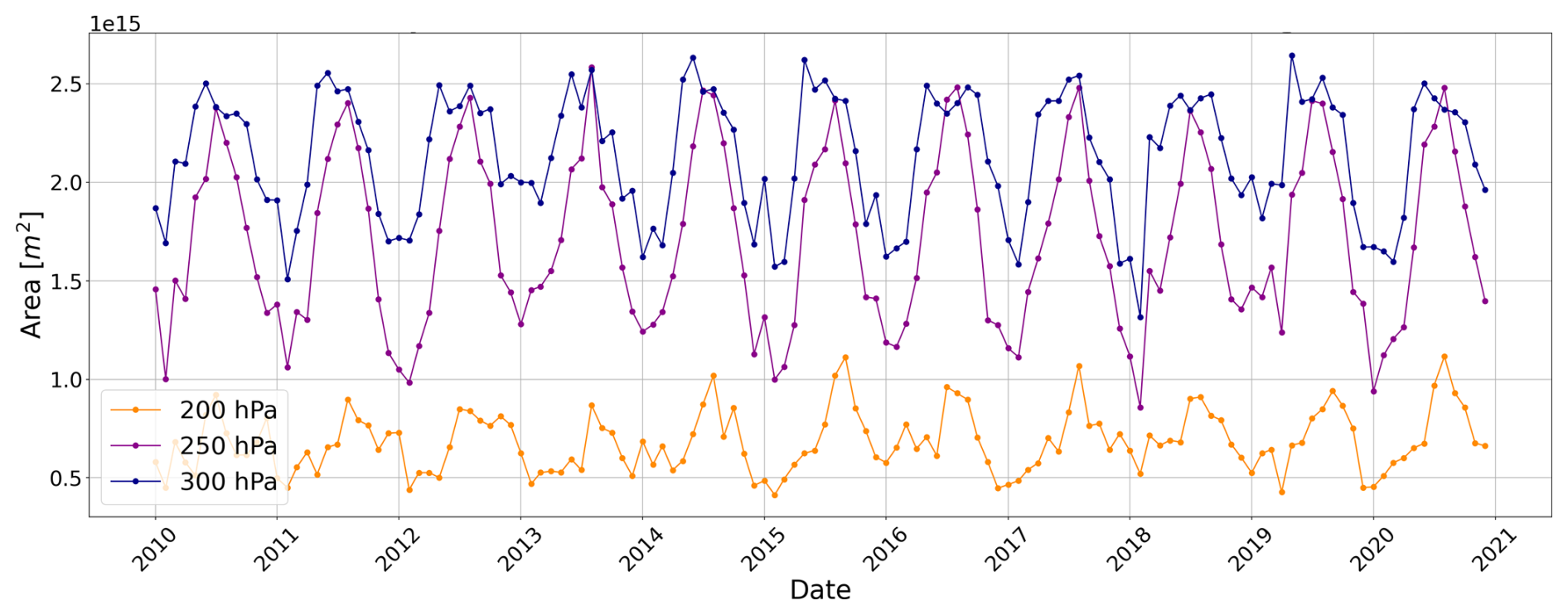
Figure 2 Monthly ISSR total area from 2010 to 2020 at pressure levels of 200 hPa (orange), 250 hPa (violet) and 300 hPa (dark blue).

In addition to the total number of ISSRs we investigate the total area of the detected ISSRs. Analogous the number of ISSRs, in Fig. 2 the total area of observed ISSRs by month on the 200, 250 and 300 hPa pressure levels in the timespan from 2010 to 2020 is shown. As for the evaluation of the total number, the area might be enhanced by counting long-lived ISSRs multiple times. The total area is largest at the lowest altitude (i.e. pressure level p=300 hPa), and is decreasing with increasing altitude. The highest total area in one month was observed in May 2019 with a summed area of 2.65×10⁹ km² at pressure level p=300 hPa. On the same pressure level the minimum of 1.32×10⁹ km² is found in February 2018. At the highest altitude level (pressure level p=200 hPa) the area is strongly reduced compared to the other two levels, which have comparable area values. At p=200 hPa the month with the highest total area of supersaturation in respect to ice is July 2020, summing up to 1.12×10⁹ km². February 2015 at this pressure level constitutes the absolute minimum observed on all pressure levels with 0.41×10⁹ km². Like the total number, the area also shows a seasonal cycle. We find maximum values in the summer months, and minimum values in the winter months, similarly to the investigations of the total number of ISSRs. The cycle is most pronounced in the two lower levels (p=300 hPa and p=250 hPa), while for the highest level (p=200 hPa) the variation is weak but still apparent. In summer, the total area of ISSRs at p=250 hPa is approaching values comparable to (p=300 hPa. This comparability only holds for the area maximum in summer, whereas the area decreases more strongly at p=250 hPa compared to p=300 hPa in winter.

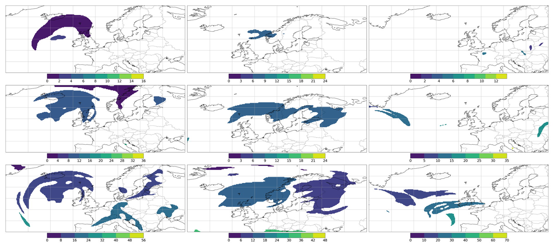
Figure 3 Exemplary ISSRs at pressure levels p=200 hPa, p=250 hPa, p=300 hPa (top to bottom) at three different times (3 columns) in January 2010. Colors are used to distinguish between individual ISSRs.

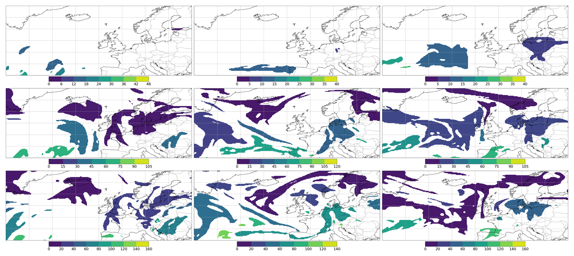
Figure 4 Exemplary ISSRs at pressure levels p=200 hPa, p=250 hPa, p=300 hPa (top to bottom) at three different times (3 columns) in July 2019. Colors are used to distinguish between individual ISSRs.

In Fig. 3 examples of ISSRs at the three different pressure levels over the North Atlantic region are presented for three times in January 2010, giving a snapshot. A similar example is shown in Fig. 4 for one snapshot in July 2019 (3 times). In winter the ISSRs are discernibly more compact and cover a limited area (Fig. 3). At the highest altitudes (i.e. at pressure level p=200 hPa) there are very few ISSRs while at lower altitudes (higher pressures) more ISSRs can be seen. In winter the tropopause is located at lower altitudes, thus the pressure level p=200 hPa is (most likely) completely contained in the stratosphere. In contrast, in July we find widespread and frayed ISSRs at all three pressure levels (Fig. 4). Even at p=200 hPa ISSRs can be found, since during summer the tropopause is located at higher altitudes and ice supersaturation is present there.

To gain a better understanding of the correlation between ISSR count and area in relation to seasons, we calculated the mean ISSR area from the corresponding number and area statistics. The results are shown as timeseries in Fig. 5.

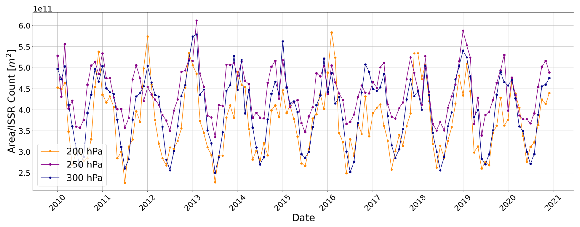
Figure 5 Averaged area as calculated from the number and areas of ISSRs, determinated in the evaluation in Sect. 3.1.

We see a pronounced seasonal cycle in the mean area of ISSRs with a very distinct maximum in winter (mean values $\overline{A}\sim \mathrm{5}$–6×10¹¹ m²) and a clear minimum in summer (mean values $\overline{A}\sim \mathrm{2.5}$–3×10¹¹ m²). Assuming a purely spherical shape, this would translate into a factor of $\sqrt{\mathrm{2}}$ for the radii. This behavior hints at two different formation mechanisms dominating in summer and winter respectively.

While the average area per ISSR on the 200 and 300 hPa levels show good agreement across all seasons, this ratio is noticeably larger at 250 hPa during summer. This feature does not represent an outlier but can be explained by jointly considering the number count and total area. In winter, both the number count and total area at 250 hPa are substantially lower than at 300 hPa. During summer, the total area at both levels is comparable, despite a lower number count at 250 hPa. Consequently, the ratio of total area to number count is increased at 250 hPa in summer. The underlying cause of this feature is the 250 hPa level being recurrently located within both the upper troposphere and lower stratosphere depending on the season. In contrast, 200 hPa remains predominantly above and 300 hPa predominantly below the tropopause throughout the year (Spichtinger et al., 2003a).

The different shape of ISSRs in winter and summer, as observed in Figs. 3 and 4, can also be seen in the (statistical) investigations of the fractal dimension, as described in the next section.

3.2 ISSR Dimension

The fractal dimensions for all ISSRs in the data set are derived using the methods explained in Sect. 2.2 and Appendix A. We calculate area and perimeter for each detected ISSR (i.e. each connected “island”) and determine the fractal dimension by using all data of a certain pressure level for a whole month in a double logarithmic scatter plot. In Fig. 6 an example is shown for January 2017, in the Supplement another example provided for July 2017).

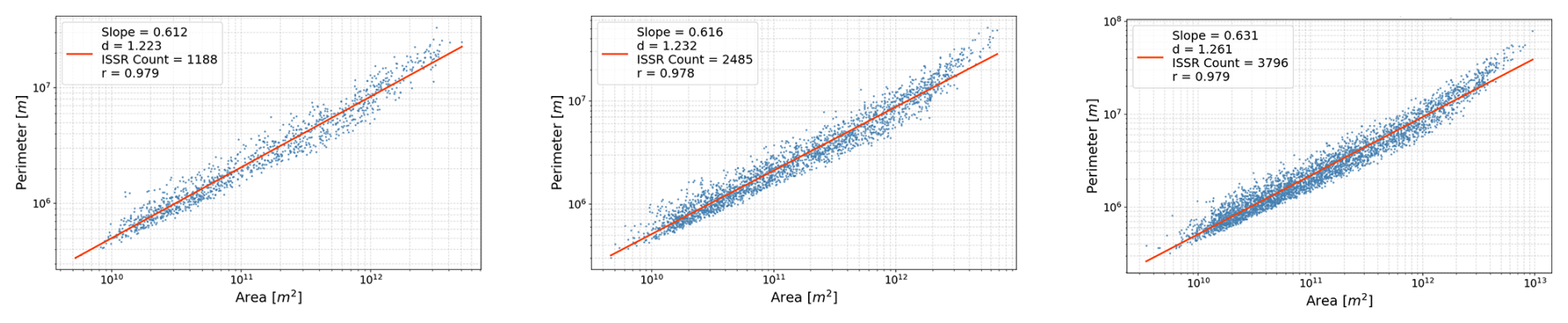
Figure 6 Determination of the fractal dimension via fits to the area-perimeter relation (Eq. 4) for January 2017. Blue dots indicate the data points (tuple (A,P)), red lines are the fits from linear regression. Left: Pressure level p=200 hPa; Middle: Pressure level p=250 hPa; Right: Pressure level p=300 hPa.

In the scatter plots the data is confined to a linear point cloud. There is a perceptible change in slope at areas of $A\sim \mathrm{2}\times {\mathrm{10}}^{\mathrm{12}}{\mathrm{m}}^{\mathrm{2}}$. As this signature is weak, we do not separate these two regimes in this evaluation. It might be related to the fact that the horizontal extent of objects on isobaric surfaces in the Earth's atmosphere is limited by the finite surface of the Earth. This can also be seen in the investigations of the horizontal extents in Sect. 4. A linear regression is applied to the complete dataset of each respective month, and the resulting slope is used to determine the respective fractal or self-similar dimension, as indicated in Eq. (4). We find values in the range D∼1.18–1.375, i.e. values well above the value of D=1 for a geometric object.

As illustrated in the simple examples presented in Appendix B, the increase of fractal dimension for larger objects might be driven either by more elongated objects (for example the systematically stretched rectangular) or by more frayed objects. Both reasons seem to be plausible from the presented snapshots in Figs. 3 and 4, but a clear attribution is not possible.

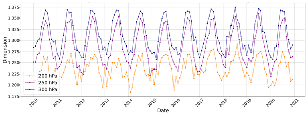
Finally, we determine the annual evolution of the fractal dimension as obtained from monthly data at different pressure levels; the results are represented in Fig. 7. We see a clear separation by vertical levels. For each month, the fractal dimensions are ordered, with the smallest value assigned to pressure level p=200 hPa, followed by the medium value at pressure level p=250 hPa and the highest value at pressure level p=300 hPa. The fractal dimensions of the observed ISSRs are in the ranges D∼1.18–1.29 (p=200 hPa), D∼1.22–1.36 (p=250 hPa), and D∼1.26–1.375 (p=300 hPa). All fractal dimensions D show a strong seasonal cycle with maxima during summer and minima during winter. The amplitude for the cycles is largest for the pressure level p=250 hPa, followed by a slightly reduced amplitude for the pressure level p=300 hPa. The variation of the monthly fractal dimension is smallest for the pressure level p=200 hPa, but it is still well pronounced. The correlation coefficient for the linear fit indicating the quality of the fits by the linear regression are relatively high (r²≥0.95). Thus, we can conclude that these results are robust and constitute a new and pronounced feature of ISSRs. The influence of the grid resolution (i.e. grid coarsening) on the derived fractal dimension is discussed in the Supplement. Unless otherwise indicated, all plots and results are based on ERA5 data at a horizontal resolution of 0.25° in both longitude and latitude.

The large seasonal variation of D might point to different physical formation mechanisms, as discussed below.

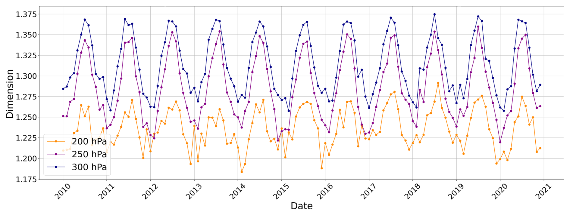
Figure 7 Fractal dimensions at three pressure levels (200 hPa in orange, 250 hPa in violet, and 300 hPa in dark blue) in a monthly resolution for the time span of 11 years of ERA5 data.

Although this is the first study investigating the fractal nature of ISSRs, we can try to compare our results to similar studies on fractal dimensions, e.g., for high clouds observed in satellite data and models with global storm resolving resolutions. Since ice clouds form in ISSRs, there should be a comparable relationship. Batista-Tomás et al. (2016) evaluated satellite data (spatial resolution of 1 km) of (ice) clouds and found a fractal dimension of $D=\mathrm{1.37}\pm \mathrm{0.02}$ for high cirrus clouds, and a fractal dimension of $D=\mathrm{1.18}\pm \mathrm{0.05}$ for cumulonimbus clouds. These values are in the same range as values of D found in this study, showing clear fractal properties of clouds. Christensen and Driver (2021) investigated satellite data (5 km grid) and high resolution model data (initialized using the ECMWF 9 km analysis data, linear resolution of 2.5 to 7.8 km for the core ensemble) and found fractal dimensions in the range D∼1.35–1.45 for the satellite data, and D∼1.27–1.53 for the different (high-resolution) models, which are also comparable to our findings. Since we are not distinguishing between cloudy and clear air inside ISSRs, there might be a mixture of different signatures of clouds and cloud free air massses (constituting all ISSRs). Nevertheless, these results show that ISSRs exhibit a clear signature of self-similarity.

4 Horizontal extent of ISSRs

Although ISSRs are quasi 2D objects on isobaric surfaces, a common measure for ISSRs is the so-called pathlength. The pathlegth is the distance traveled by an aircraft within an ISSR. Gierens and Spichtinger (2000) first investigated pathlength statistics of ISSRs using data from the MOZAIC project (Marenco et al., 1998), this study was later extended by Spichtinger and Leschner (2016) for the IAGOS data set (Petzold et al., 2015). The pathlengths, constituting 1D tracks through 3D objects, give a first idea about the horizontal extent and the shape of ISSRs. Since we use quasi 2D data (at pressure levels) in this study, we can generate artificial pathlengths in order to simulate the distribution of realistic pathlengths. These can be used in two different ways. First, using zonal and meridional directions (i.e. East-West, North-South, respectively), we can statistically investigate the horizontal extent (or span) of ISSRs in a systematic but less realistic way. Second, we can generate more realistic pathlengths in using simulated flight tracks along geodesics between frequently used airports. These tracks are chosen specifically to cover routes also included in the IAGOS project (Petzold et al., 2015).

The zonal and meridional extents are not measured as a means to obtain the largest extent in one direction, but rather to generate a full set of spans along latitudes/longitudes touched by the respective ISSR. Thus, the ISSR is measured in “slices” with a spacing of 0.25°. This procedure is carried out for both zonal and meridional directions. The resulting data is separated by seasons, i.e. summer (JJA) and winter (DJF), and is used to derive statistical distributions of the horizontal extent of ISSRs.

The data used deliberately does not include measurements shorter than 27 km, as this is approximately the longest single-pixel length that can be measured in the target region. Including distances below that threshold is not meaningful, since this would introduce artificial biases stemming from different pixel sizes at different locations, leading to artificial breaks of regimes. Note that we still use the data set with the restriction of a minimum of 24 pixels per ISSR. This might also crucially reduce the number of small ISSRs in the evaluation, but this is consistent with our investigations in Sect. 3.

Former investigations of pathlength statistics showed Weibull-type distributions (Gierens and Spichtinger, 2000; Spichtinger and Leschner, 2016), or at least the distributions could be well represented using Weibull-type fits. We emphasize that the application of the Weibull distribution in this context is purely empirical. In contrast to classical extreme-value statistics, we do not consider maxima of underlying distributions, but rather the full population of pathlengths. Therefore, a strict interpretation in the framework of extreme-value theory is not appropriate here. Instead, the Weibull distribution is used as an empirical fitting function that provides a good representation of the observed distributions and allows for a compact characterization via its parameters, which is consistent with above mentioned studies studying ISSR distributions.

The probability density function of a Weibull distributed random variable x is given by $f\left(x\right)=\mathit{\gamma }p{x}^{p-\mathrm{1}}\exp (-\mathit{\gamma }{x}^p)$ with shape parameter $p\in {\mathbb{R}}_{+}$ and scale parameter $\mathit{\gamma }\in {\mathbb{R}}_{+}$. The parameter p determines the overall shape of the distribution. It can be obtained by using a Weibull plot (and the cumulative distribution $F\left(x\right)=\mathrm{1}-\exp (-\mathit{\gamma }{x}^p)$) with linear regression. The slope of the regression line is the parameter p. For more details about Weibull plots we refer to Appendix D.

4.1 Span along Longitude

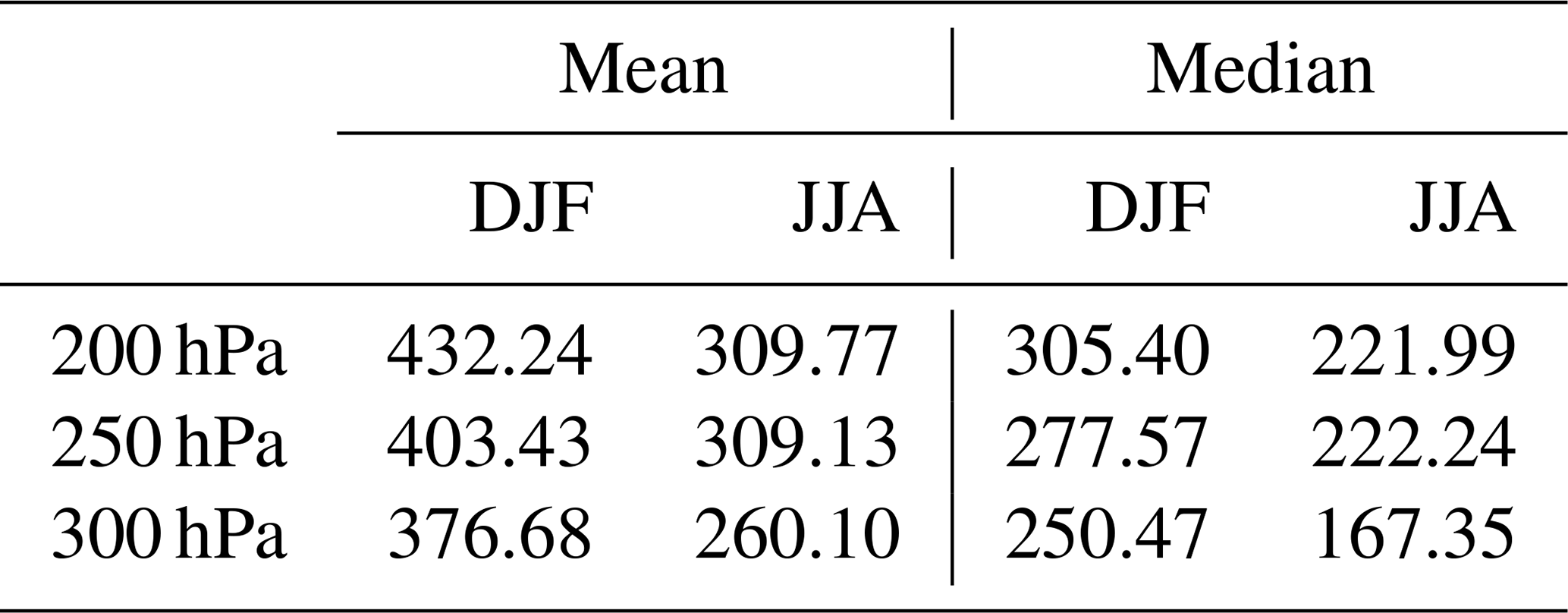
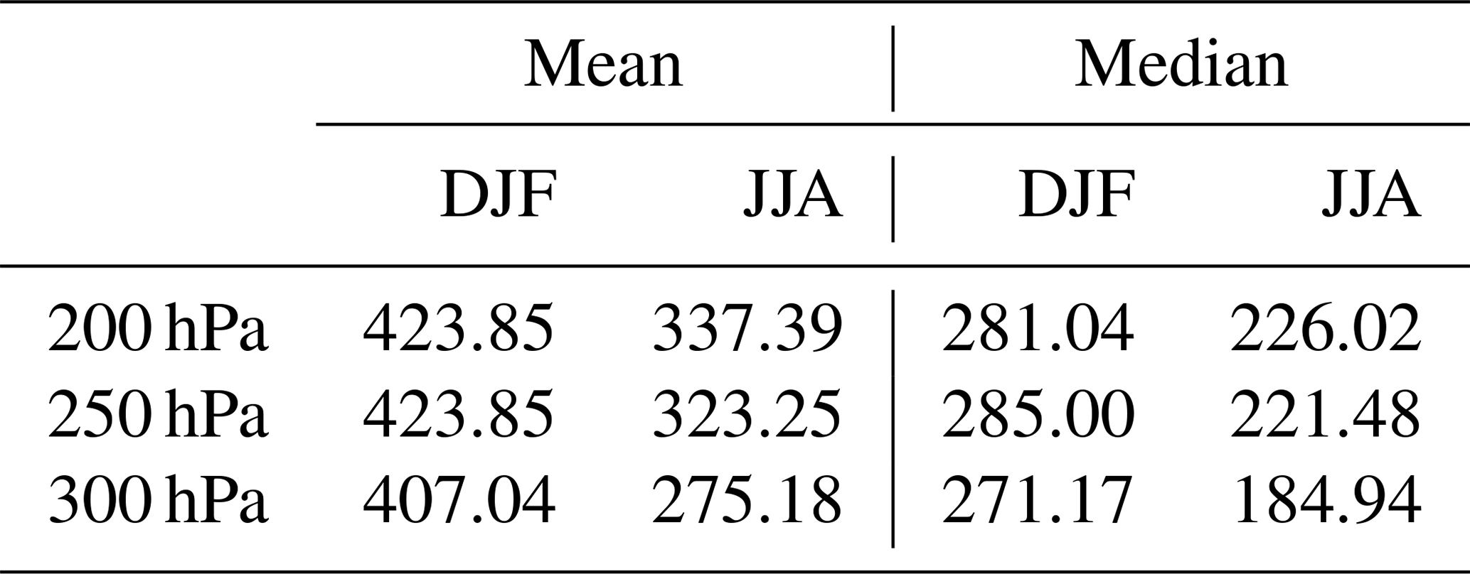
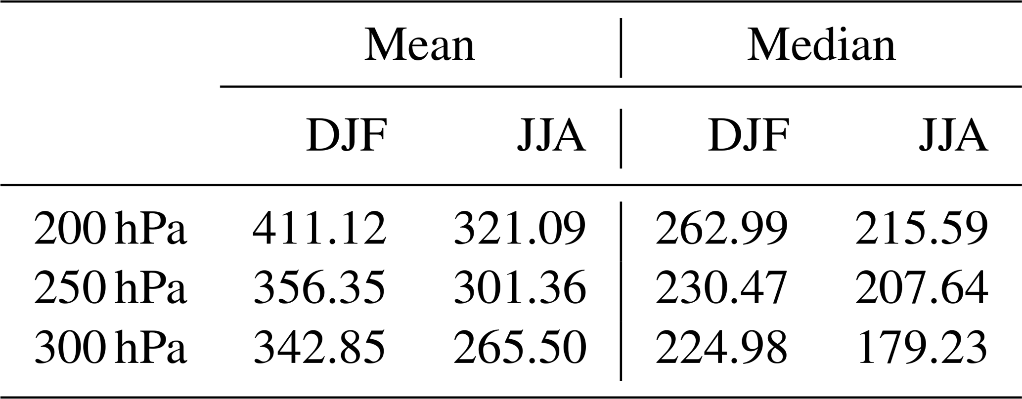
First, we investigate the meridional slices, i.e. pathlengths along longitudes. Since the major variation of horizontal extents is between winter and summer, we exclusively show these results in all respective figures. The probability density functions for winter and summer, differentiated into three pressure levels are shown in Fig. 8. The mean and median values are reported in Table 1.

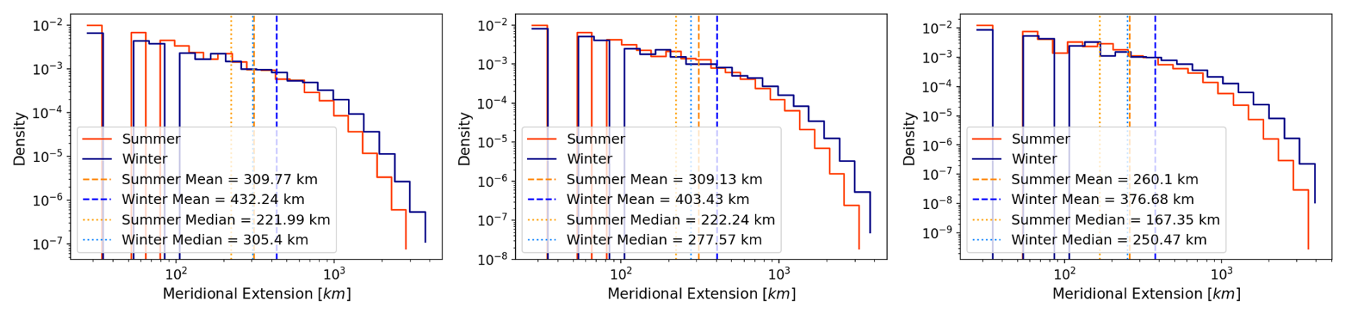
Figure 8 Distributions of meridional span (i.e. pathlengths in North-South direction) for summer (JJA, orange colors) and winter (DJF, blue colors). Mean values are indicated by vertical dashed lines, median values are indicated by vertical dotted lines. Left: 200 hPa, Middle: 250 hPa, Right: 300 hPa.

For all pressure levels p=200/250/300 hPa, the mean meridional extent of ISSRs is significantly higher in winter compared to the summer months. While the density does not differ substantially between seasons for ISSRs up to a size of approximately 10³ km, the disparity between summer and winter inflates with increasing measured span. The absolute mean span increases with decreasing pressure (i.e. with rising altitude levels). The relative difference comparing summer and winter slightly increases with higher pressure (i.e. lower altitudes). All values are reported in Table 1. The strong seasonal cycle is present in both the mean values and the extreme tails of the distributions. In winter, the season with maximum mean values, a clear enhanced probability of finding extremely large pathlengths (i.e. enhanced values in the tail of the distribution) can be seen, whereas the probability of extremely large pathlengths is reduced in summer. The histograms are not symmetric but right-skewed, so the mean is pulled upward by few large ISSRs. The median is more robust and thus more suitable to assess the typical 2D features of ISSRs. The median behaves similarly to the mean in that it generally decreases with increasing pressure, the exception being a minor increase from 200 to 250 hPa in the summer months.

Table 1 Mean and median values of the meridional span (pathlength in North–South direction, in km) for DJF and JJA at different pressure levels.

The data shows two regimes with roughly linear correlation but different slopes in the Weibull plots (i.e. in the respective values of parameter p) in Fig. 9. Thus, there are two distinct distributions superimposed in the histograms. The transition between these regimes is roughly located at $L\sim \mathrm{2}\times {\mathrm{10}}^{\mathrm{2}}\mathrm{km}$. For the smaller ISSRs we find values of p∼1.5, whereas the distribution is close to an exponential distribution (p∼1) for the larger ISSRs.

The presence of two clearly separated size regimes suggests different formation mechanisms of ISSRs operating at distinct spatial scales, i.e. synoptic-scale vs. localized on mesoscales, leading to characteristic horizontal extents. This hypothesis is subject to further investigation, since an in depth analysis is out of scope of this study.

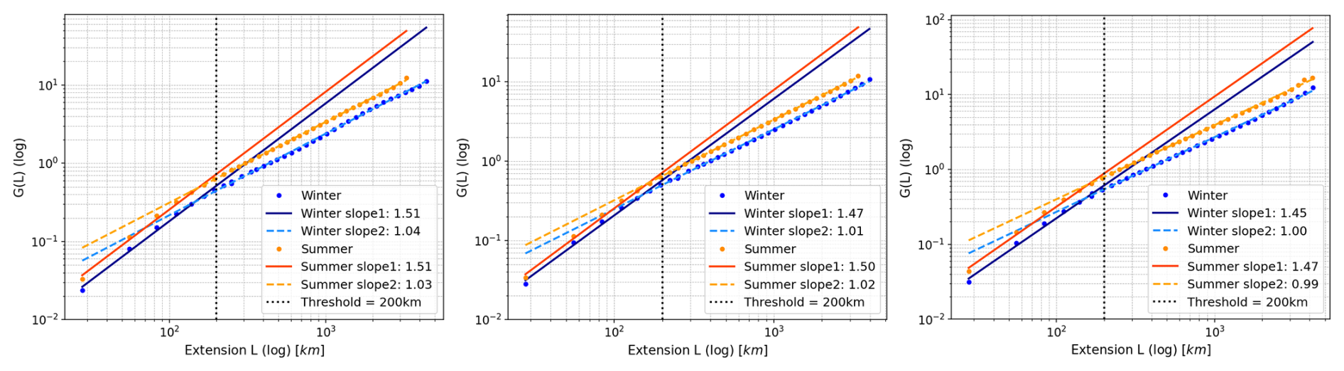
Figure 9 Weibull plots for the pathlength distributions in North-South direction. The linear regression fit is shown for the regimes of pathlengths smaller and larger than $\sim \mathrm{2}\times {\mathrm{10}}^{\mathrm{2}}\mathrm{km}$ (dashed vertical line). Blue/orange colors indicate winter/summer data, respectively. The fits to the different regimes are represented by a dashed and a solid line. Left: 200 hPa, Middle: 250 hPa, Right: 300 hPa.

4.2 Span along Latitude

Alike investigating the meridional slices along longitudes, we now investigate horizontal extents along latitudes, i.e. slices in zonal (East–West) direction within ISSRs. The probability density functions for the two seasons (summer/winter), separated into three pressure levels, are shown in Fig. 10.

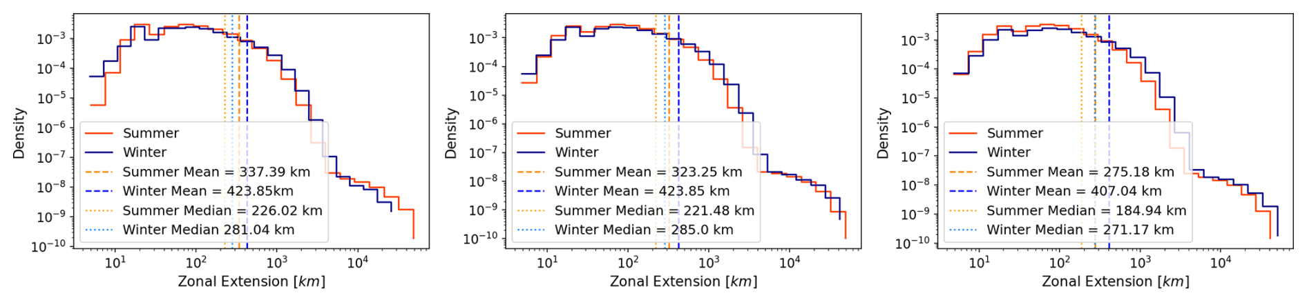
Figure 10 Distributions of zonal span (i.e. pathlengths in East-West direction) for different seasons, i.e. summer (JJA, orange colors) and winter (DJF, blue colors). Mean values are indicated by vertical dashed lines, median values are indicated by vertical dotted lines. Left: 200 hPa, Middle: 250 hPa, Right: 300 hPa.

The distribution of measured zonal distances shows almost identical qualitative characteristics as the meridional counterpart. We see a strong decrease in frequency of occurrence for spans larger than the mean values. In contrast to the meridional distributions, there is an additional very small mode at very large spans (L∼10 000 km), indicating the occurrence of very few very large ISSRs in East-West direction. This difference can be explained by pathlengths in meridional direction being limited to the 30–80° N range we study, while zonal pathlengths can theoretically extend to the length of the latitude. For all pressure levels, the mean span is significantly higher in the winter months compared to the summer months. Differences in the distribution of spans by season are most clear for larger spans. The mean generally decreases slightly with a higher pressure level. The decrease in mean span with higher pressure is more evident in the summer months. Analogous to the meridional observations, the median is consistently lower than the mean. The median increases marginally from 200 to 250 hPa in winter but behaves analogous to the mean in all other instances. It is lowest at the highest pressure level. As with the meridional span, the distribution is right-skewed. All values are reported in Table 2. We see the same feature of enhanced probability for extremely large pathlengths during winter and reduced probability during summer.

Table 2 Mean and median values of the zonal span (pathlength in East–West direction, in km) for DJF and JJA at different pressure levels.

In Fig. 11 we investigate the Weibull plots for the distributions. For the zonal spans, three distinct regimes are visible. There is a regime of very small spans (up to L∼10² km), without a clear Weibull signature in the Weibull plot. In addition, there are two further regimes, separated at values $L\sim \mathrm{2}\times {\mathrm{10}}^{\mathrm{3}}\mathrm{km}$, which show linear behavior in the Weibull plots, thus indicating two different regimes clearly distinguishable by a different Weibull parameter p. The regime of intermediate spans of ISSRs results in an almost exponential distribution (Weibull parameter p∼1), whereas the regime of very large spans shows a Weibull characteristic with parameter p∼0.2. This characteristic remains virtually identical across seasons.

The regime of very small pathlengths might be an artifact of the evaluation. The real area of a pixel (or grid point) depends crucially on the latitude. Scanning high latitude circles will systematically produce small horizontal sizes for ISSRs consisting of few pixels.

The tiny mode of very large spans of ISSRs of orders up to almost latitudinal circumference might indicate the impact of synoptic and large scale weather systems, triggering atmospheric flows in the zonal direction with a persistent vertical upward motion, thus leading to a persistence of ice supersaturation in the UTLS. The upper bound of such synoptically driven ISSRs is given by the circumference of the Earth at certain latitudes.

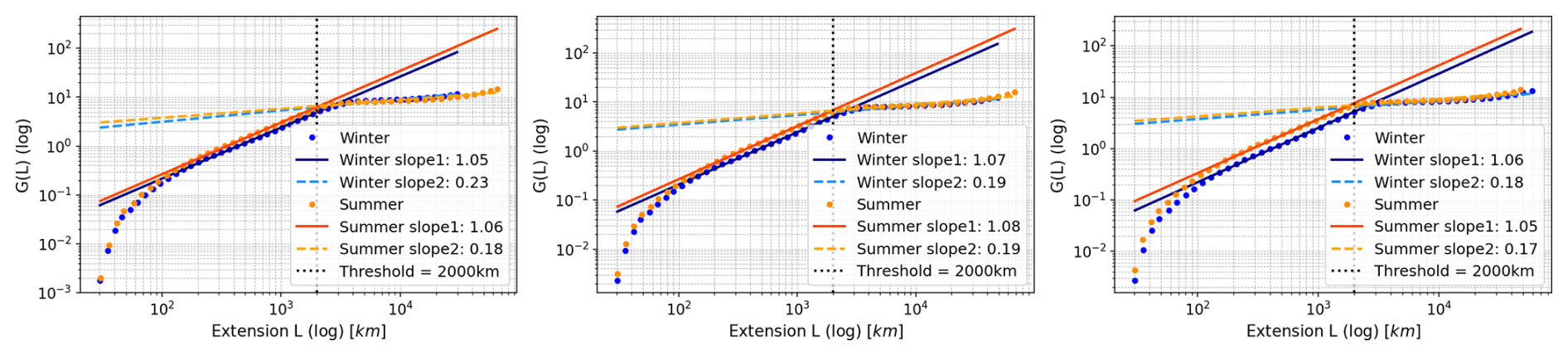
Figure 11 Weibull plots for the pathlength distributions in East-West direction. The linear regression fit is shown for the regimes of pathlengths smaller and larger than $L\sim \mathrm{2}\times {\mathrm{10}}^{\mathrm{3}}\mathrm{km}$ (dashed vertical line). with a clear scale break at $L\sim \mathrm{2}\times {\mathrm{10}}^{\mathrm{3}}\mathrm{km}$ (indicated by a dotted line). Blue/orange colors indicate winter/summer data. The fits to the different regimes are represented by a dashed and a solid line. Left: 200 hPa, Middle: 250 hPa, Right: 300 hPa.

4.3 Span along modeled aircraft tracks (pathlengths)

In addition to the rather artificial longitudinal and latitudinal measurements, realistic pathlengths are investigated. In lieu of real in situ measurements, tracks along commercial aircraft routes are investigated. We exemplarily chose three transatlantic flight routes based on the flight tracks frequently found in the IAGOS data (Petzold et al., 2015). The three tracks (i.e. direct flight routes Berlin–Chicago, Frankfurt–Atlanta, and Paris–Miami) are assumed as geodesics on a sphere (Fig. 12). The pathlengths are obtained by measuring the distance along the sections of ice supersaturation on the flight track from airport to airport.

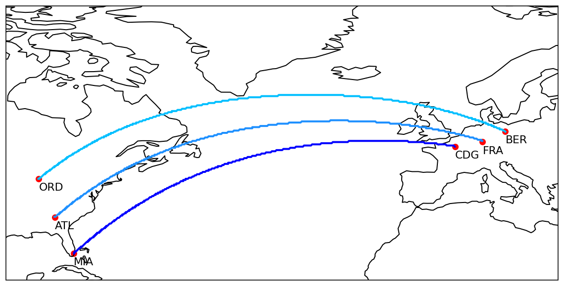
Figure 12 Typical flight routes of commercial air traffic for some important airports in the US (Chicago, Atlanta, Miami) and Europe (Berlin, Frankfurt, Paris). These flight routes can be seen in the measurement data from the IAGOS project.

The histograms (Fig. 13) show numerical artifacts for small ISSRs. We find the same features of pathlength statistics for mean values and distributions as in Sect. 4.1 and 4.2. The winter months yield the highest mean pathlengths while summer returns the shortest mean distances. For all seasons there is an increase of mean and median values with increasing altitude. The highest mean/median pathlengths can be found at the highest level (p=200 hPa), and the lowest values at p=300 hPa with intermediate values at the level p=250 hPa. The distributions mostly agree for the two seasons, with a larger deviation for the largest pathlengths. During winter, there are more large ISSRs than during summer. The mean and median values of the pathlength distributions are represented in Table 3. The mean exceeds the median in all instances.

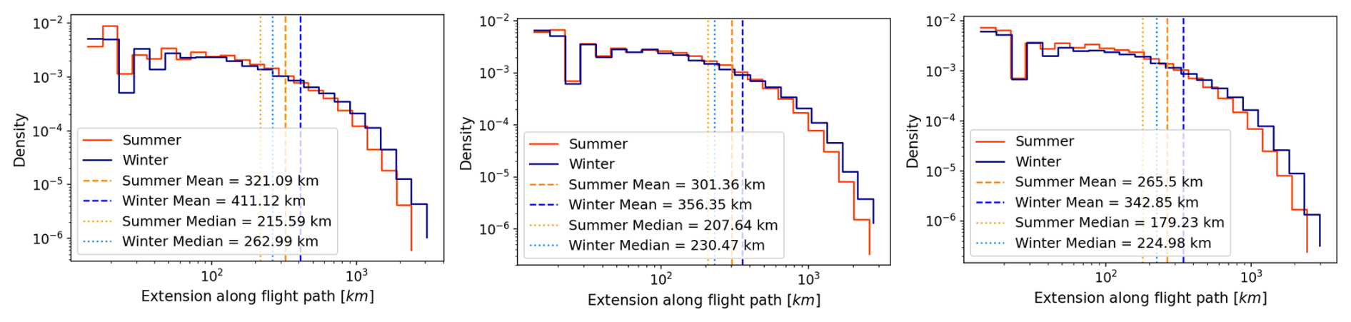
Figure 13 Distributions of realistic pathlengths for different seasons as simulated by assuming common flight tracks (as shown in Fig. 12) for different seasons, i.e. summer (JJA, orange colors) and winter (DJF, blue colors). Mean values are indicated by vertical dashed lines, median values are indicated by vertical dotted lines. Left: 200 hPa, Middle: 250 hPa, Right: 300 hPa.

Table 3 Mean and median values of pathlengths (i.e. artificial flight tracks, in km) for DJF and JJA at different pressure levels.

In the evaluation of the Weibull plots (Fig. 14), we find two different regimes of distinct Weibull distributions with different values of p, separated at pathlengths L∼10² km, analogous to the meridional extents. The difference in the regimes is more pronounced compared to the former evaluation, and the signal of the very large zonal extents is missing in this evaluation. This is expected, as the largest possible extent is the distance between airports. As before, we overlook the very small pathlengths in the linear regression. For both regimes, the seasonal cycle is not strongly pronounced. In the small pathlengths regime, we find values p∼1.95, whereas in the regime of large pathlengths, the values are close to an exponential distribution, i.e. p∼1. This signal is very robust, with almost no seasonal variation in the parameters or with respect to the different levels.

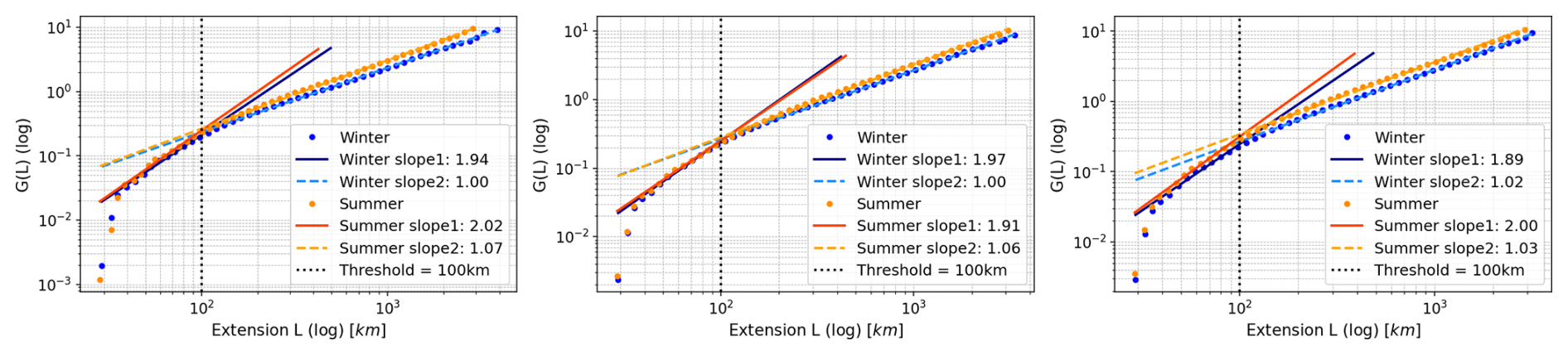
Figure 14 Weibull plots for the pathlength distributions of realistic pathlengths simulated by common flight tracks. The linear regression fit is shown for the regimes of pathlengths between 40 and ∼10² km and pathlengths larger than L∼10² km, this threshold being indicated by a dotted line. Blue/orange colors indicate winter/summer data, respectively. The fits to the different regimes are represented by a dashed and a solid line. Left: 200 hPa, Middle: 250 hPa, Right: 300 hPa.

4.4 Agreement of pathlength distributions

The results of the longitudinal, latitudinal and pathlength measurements agree well with another. The observation of the summer months yielding the shortest and winter the longest mean distances generally holds true across methods. This agreement applies to most results in terms of dependence on pressure level as well. The mean span is generally larger at lower pressures, i.e. higher up in the atmosphere. While this is always true for the comparison between levels p=200 hPa and p=300 hPa, in the intermediate level p=250 hPa some variations can be seen. The mean values for zonal extents are generally larger than those for the meridional extents and the flight track pathlengths. This feature likely stems from ISSRs usually extending more in East-West direction (as shown in Figs. 3 and 4), driven by the mean large scale flow.

The results of the simulated IAGOS flights have a larger qualitative agreement with the meridional extents. In both cases, there is a scale break at L∼10² km , separating two different modes of Weibull distributions. The tiny mode of exceptionally large spans as found in the zonal slices cannot be detected in the pathlengths of realistic flight tracks. These very few, very large ISSRs are mostly elongated into zonal direction and the maximum of possible pathlength is limited by flight track length.

The distributions as well as the mean (and median) values of the simulated pathlengths compare qualitatively well with the former investigations of pathlengths as obtained from aircraft measurements (Gierens and Spichtinger, 2000; Spichtinger and Leschner, 2016). The mean (and median) values as obtained from the ERA5 data are generally larger than those of aircraft data. This is not surprising, since the aircraft data has a much higher temporal (and thus spatial) resolution. The Weibull shaped distributions can be seen in all evaluations with a varying degree of prominence of a scale break at pathlengths L∼10² km. The fitted Weibull parameter of the distributions differ between aircraft data and ERA5 evaluation. The general feature of a smaller slope for pathlengths below the scale break and a higher slope for pathlengths above the scale break is present in all evaluations. The difference in slopes for aircraft vs. ERA5 data is likely due to the different resolutions of the data sets. Finally, we see that the range of the obtained distributions of pathlengths is roughly the same in all investigations (ranging from few 10 km up to ∼5000 km).

5 Discussion and conclusions

Ice supersaturated regions in the UTLS are important potential formation regions of ice clouds and contrails. For a better understanding of these regions on different scales and resolutions, we investigated ISSRs in ERA5 data as “macroscopic” and quasi two dimensional objects on pressure levels in the UTLS. We can summarize the main findings as follows:

ISSR characteristics tend to have seasonal cycles. We can observe this in both the number and total area of ISSRs. The number of ISSRs is largest during summer and smallest during winter across all pressure levels. The total area covered by ISSRs shows the same behaviour. While the total area is largest in summer, the average area per ISSRs is significantly smaller during the summer months. In addition to their seasonal variability, ISSR number and area display a distinct vertical structure. The number of ISSRs is highest for lower altitudes and declines with decreasing pressure. We find the same vertical layering for the total area of ISSRs with a decrease in total area with increasing altitude. The vertical variation of total area itself is subject to a seasonal cycle. Area values at p=250 hPa approach those at p=300 in summer but drop significantly lower than the latter in winter. The average area per ISSR shows little vertical variability with the exception of higher values in summer at p=250. This effect can be attributed to the larger amplitude in total area at that pressure level. The larger amplitude is a feature caused by the seasonally differing altitude of the tropopause (Spichtinger et al., 2003a).

The calculated values of fractal dimension of ISSRs are in the range $\mathrm{1.175}\le D\le \mathrm{1.375}$. A pronounced seasonal cycle is evident for the fractal dimensions as well, producing larger values in summer and smaller values in winter. This signal appears on all considered pressure levels. The fractal dimensions also show a distinct vertical layering with largest values for low altitudes and lower values for high altitudes.

In the evaluation of the horizontal extents of ISSRs, i.e. deriving pathlengths in various ways (artificial East-West and North-South spans vs. realistic flight paths), the seasonal variation is maintained. Generally, we find smaller pathlengths during summer (smaller mean values, less extremes), whereas during winter the pathlengths are generally larger (larger mean value, more large pathlengths). This feature is robust for all evaluated pressure levels. In the pathlengths statistics, we find different regimes, as also indicated by different values of the shape parameter p in the Weibull plots, indicating a superposition of two different Weibull distributions.

As can be seen in the simple exercise in Appendix B about changes in fractal dimensions, more elongated or even strongly frayed objects have larger fractal dimensions than their strictly geometric counterparts (i.e. D>1). As indicated by the snap-shots in Figs. 3 and 4, in summer the ISSRs are more elongated and more frayed than in winter. The fractal dimension is larger for ISSRs in summer, thus we expect more frayed/elongated objects. In turn, these objects result in shorter pathlengths, as traversing them generally involves smaller cross sections of ice supersaturation. On the other hand, ISSRs in winter have smaller fractal dimensions, thus suggesting a more compact shape. This is consistent with the pathlength statistics, as traversing more compact objects results in fewer short pathlengths and, on average, larger cross sections. Thus, the seasonal cycles of fractal dimensions and pathlengths are physically consistent.

Consistent with our initial hypothesis, the analysis of the area–perimeter relationship demonstrates that ISSRs in the UTLS exhibit self-similar (fractal) behavior.

The strong contrast between fractal properties of ISSRs for different seasons suggest different formation processes. For this we might also take into account the seasonal fluctuation in the number of ISSRs with a peak in summer. A possible explanation is the transportation of water vapor into the UTLS by convection during the summer months. A multitude of convection sites causes high ISSR numbers while the winter months are dominated by low pressure areas and frontal systems. The ascending air flow of the warm conveyor belt causes a connected area of supersaturation. This hypotheses is supported by the shorter mean latitudinal and longitudinal spans in summer compared to winter months. It is further corroborated by the pronounced seasonal cycle in the mean area of ISSRs. The distinct maximum in winter and clear minimum in summer is consistent with the proposed formation mechanisms: convective processes in summer produce more localized ISSRs, whereas large-scale dynamics in winter lead to more extended structures. Extending this hypothesis to the seasonal variation in the fractal dimension, particularly during the period with the lowest values in summer, provides two possible interpretations. One perspective suggests that convective sites lead to ISSRs with frayed boundaries, resulting in long perimeters compared to the smoother edges of ISSRs caused by frontal activity, i.e. large scale dynamics. An alternative interpretation posits that multiple convective “bubbles” occurring in close proximity may be collectively labeled as a single ISSR. This would lead to elevated perimeters attributed to their intricate structure and the added internal perimeter created by holes that segregate convective regions.

In addition, the scale break in the Weibull plots of the pathlengths at $L\sim \mathrm{2}\times {\mathrm{10}}^{\mathrm{2}}\mathrm{km}$, which is consistent with former investigations (Spichtinger and Leschner, 2016), also suggest a possible superposition of two different populations of ISSRs. This can possibly originate in the slopes corresponding to smaller and larger ISSRs. Smaller scale ISSRs form in localized lifting phenomena like convection. Frontal activity and large scale dynamics create larger areas of supersaturation with respect to ice.

Our findings of seasonal variation and vertical layering in ISSR numbers are consistent with Reutter et al. (2020) and Spichtinger et al. (2003a). The pathlengths statistics and Weibull distributions are in good agreement with Spichtinger and Leschner (2016). Batista-Tomás et al. (2016) found similar dimension values for clouds. These consistencies with former studies allow confidence in our results. However, fractal dimensions of ISSRs have not previously been quantified systematically from ERA5 data (to our knowledge), representing a novel contribution.

When interpreting the presented results, limitations need to be considered. As the study is based on ERA5 reanalysis data, the identified ISSRs and their geometric characteristics depend on the representation of humidity and on the spatial resolution of the underlying data set. Changes due to the coarsening of the grid are discussed in the Supplement. Confirming our findings with studies on measured rather than modeled data could act as an endorsement to incorporate self-similar and fractal characteristics in other models.

Treating ISSRs as quasi 2D objects on isobaric surfaces neglects their three-dimensional nature. This does not substantially affect our confidence in the results, as previous investigations have successfully characterized ISSRs using one-dimensional pathlength statistics, whereas this study extends the analysis to two-dimensional properties.

Future studies using different definitions of fractal dimension (e.g. the Hausdorff dimension) might substantiate our understanding of the fractal properties of ISSRs. Although the results allow the hypothesis of convective influences during summer and large-scale dynamical forcing during winter, an in depth investigation of formation processes is beyond the scope of this study, but is planned as future investigation.

The impact and implications of these findings are broad. The identification of fractal structures enriches scientific inquiry by providing new tools for analysis and offering deeper insights into the complexity of natural phenomena. The self-similarity of ISSRs reshapes our understanding of ISSRs as irregular but organized spatial structures across a broad range of scales with systematic seasonal and vertical variation. This study has significance for our understanding of humidity variability in the UTLS, cirrus formation, and consequently the radiation budget of the atmosphere. The observed seasonal changes in ISSR geometry suggest that the dominant mechanisms controlling ice supersaturation vary throughout the year, with convective processes contributing more strongly during summer and large-scale dynamical lifting playing a larger role during winter. The fractal nature of ISSRs further indicates that substantial spatial variability persists across scales. As a more practical aspect of the analysis, the fractal properties of ISSRs must be taken into account for the highly discussed concepts of contrail avoidance (e.g., Petzold et al., 2025). Looking at the examples of frayed ISSRs in Figs. 3 and 4, it seems to be very optimistic that contrail avoidance might work in a meaningful, impactful or feasible way. The large amount of small ISSRs (or short pathlengths) in connection with the huge fractal objects makes it very difficult to manage efficient contrail avoidance in the Northern Hemisphere.

Appendix A: Methods for evaluation

In Fig. A1 two possible definitions of neighborhoods of points on gridded data are shown, originating from investigations with cellular automaton (Chopard and Droz, 1998). Given a 4-neighborhood (or von Neumann neighborhood), the central pixel is only connected to pixels via the four edges of the point. A 8-neighborhood (or Moore neighborhood) is defined as the central pixel being additionally connected to pixels via the diagonals¹. In our evaluation, we choose the Moore neighborhood, since the physical properties as connectivity should not depend on a grid representation, i.e. rotation of the object should result into the “same” connected object.

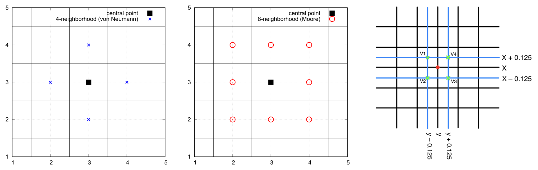
Figure A1 Two possible measures for connecting points on gridded data (Chopard and Droz, 1998). Black square: Center point. Left: Blue crosses indicate points connected to the central point using the 4-neighborhood (von Neumann neighborhood). Middle: Red circles indicate points connected to the central point using the 8-neighborhood (Moore neighborhood). Right: Assignment of area to a grid point, using a halo of ±0.125 degrees.

For the derivation of the grid point's area we use the coordinates of the point (x,y) as the center of a rectangular with vertices $(x\pm \mathrm{0.125},y\pm \mathrm{0.125})$ (see right panel of Fig. A1). The area (in square metres) is then assigned to the grid point, taking into account the latitudinal stretching of the grid. For the derivation of the perimeter, we use the four edges of the introduced rectangular, with the respective length (in metres). If there is no neighboring grid with index = 1, the edge is counted as part of the perimeter.

Appendix B: Changes in fractal dimensions

In this appendix we illustrate some effects which might have some influence on the change in the fractal dimension. We use the area-perimeter relation $P=C{A}^{\frac{D}{\mathrm{2}}}$ for the investigations. For geometric objects, the fractal dimension coincides with the classical integer values dimension, as can be seen directly for simple examples as spheres, squares, rectangulars with fixed ratio of sides.

1. Sphere: For a sphere with radius r we easily calculate the perimeter P=2πr and the area A=πr², thus leading to the derivation $\mathrm{2}\mathit{\pi }r=P=C{A}^{\frac{D}{\mathrm{2}}}=C{\left(\mathit{\pi }{r}^{\mathrm{2}}\right)}^{\frac{D}{\mathrm{2}}}=C{\mathit{\pi }}^{\frac{D}{\mathrm{2}}}{r}^D$ which immediately gives D=1 and $C=\mathrm{2}\sqrt{\mathit{\pi }}$.

2. Rectangular with fixed ratio of sides: We assume sides a and $b=d\cdot a$ with a fixed value d>0; thus, we calculate $\mathrm{2}(\mathrm{1}+d)a=P=C{A}^{\frac{D}{\mathrm{2}}}=C{\left(d\cdot a^{\mathrm{2}}\right)}^{\frac{D}{\mathrm{2}}}=C{d}^{\frac{D}{\mathrm{2}}}{a}^D$ with D=1 and $C=\frac{\mathrm{2}(\mathrm{1}+d)}{\sqrt{d}}$. Note that the example of a square (d=1) is included here, leading to C=4.

As a first example for a fractal object, we compare the fractal dimension of a square with a systematically stretched rectangular, i.e. we change the ratio between the two sides, while we proceed to larger sizes. In fact, we set a=ϵ and b=ϵ² for $\mathit{ϵ}\in {\mathbb{R}}_{+}$. Thus, we can calculate

$$\begin{array}{}\text{(B1)}& A=a\cdot b={\mathit{ϵ}}^{\mathrm{3}},P=\mathrm{2}a+\mathrm{2}b=\mathrm{2}\mathit{ϵ}+\mathrm{2}{\mathit{ϵ}}^{\mathrm{2}}=\mathrm{2}\mathit{ϵ}(\mathrm{1}+\mathit{ϵ})\end{array}$$

leading to the area-perimeter relation

$$\begin{array}{}\text{(B2)}& \mathrm{2}\mathit{ϵ}(\mathrm{1}+\mathit{ϵ})=P=C{A}^{\frac{D}{\mathrm{2}}}=C{\left({\mathit{ϵ}}^{\mathrm{3}}\right)}^{\frac{D}{\mathrm{2}}}.\end{array}$$

Applying the logarithm, we can derive an approximate value of the dimension D (and also the constant C).

Using $\log \left(P\right)=\log \left(\mathrm{2}\right)+\log \left(\mathit{ϵ}\right)+\log (\mathrm{1}+\mathit{ϵ})$, and log (A)=3log (ϵ), we obtain for the dimension

$$\begin{array}{}\text{(B3)}& \begin{array}{rl}{\displaystyle \frac{D}{\mathrm{2}}}& ={\displaystyle \frac{\log \left(P\right)-\log \left(C\right)}{\log \left(A\right)}}\\ & ={\displaystyle \frac{\log \left(\mathrm{2}\right)+\log \left(\mathit{ϵ}\right)+\log (\mathrm{1}+\mathit{ϵ})-\log \left(C\right)}{\mathrm{3}\log \left(\mathit{ϵ}\right)}}\end{array}\end{array}$$

For large ϵ we find $\log (\mathrm{1}+\mathit{ϵ})\approx \log \left(\mathit{ϵ}\right)$ and $\log \left(P\right)-\log \left(C\right)\approx \log \left(P\right)$, thus we find

$$\begin{array}{}\text{(B4)}& {\displaystyle \frac{D}{\mathrm{2}}}=\underset{\mathit{ϵ}\to \mathrm{\infty }}{lim}{\displaystyle \frac{\log \left(P\right)-\log \left(C\right)}{\log \left(A\right)}}={\displaystyle \frac{\mathrm{2}}{\mathrm{3}}}\iff D={\displaystyle \frac{\mathrm{4}}{\mathrm{3}}},\end{array}$$

and we also obtain C≈2. In the left panel of Fig. B1 the area-perimeter relation for a square and a stretched rectangular are shown together with the theoretically derived values for the fits. The systematically stretched rectangular turns into a more line-shaped geometric object, thus changing the fractal dimension to larger values.

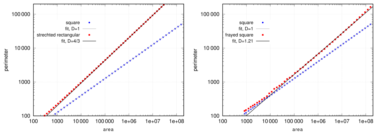
Figure B1 Examples of fractal dimension for 2D objects. Left: square vs. stretched rectangular. Right: square vs. frayed square. The fractal dimension of the frayed square is determined using linear regression to the data points in logarithmic scale. The fits to the other objects are based on the theoretically obtained values.

As a second example, we investigate a square, with a systematically frayed boundary leading to a slightly smaller area but to a strongly enhanced perimeter. A regular, unfrayed square would yield a (fractal) dimension of D=1. For the frayed square, we see that the fractal dimension is also enhanced, leading to values of about D∼1.21. The scatter plot of the normal square and the frayed square, respectively, is shown in the right panel of Fig. B1, together with the linear fit via regression. These two mechanisms (stretching and fraying) can for instance serve for changing fractal dimensions of “two dimensional” geometric objects.

Appendix C: Potential errors for gridded data: Overestimation of perimeters

It is well known that the calculation of perimeter on gridded data lead to overestimation of this quantity (Imre, 2006). However, it is not completely clear if and how the area-perimeter relation might change due to this error. Exemplarily, we investigate this for a sphere. We calculate the area and perimeter according to the methods explained above and compare these values with the analytically calculated quantities. The area-perimeter relations are represented in Fig. C1.

Despite a systematic shift in perimeters, the resulting fractal dimension D∼0.999564 (as a linear fit to the double logarithmic scatter plot) is very close to the analytically determined “fractal” dimension D=1. Thus, we are confident that the systematic overestimation of perimeters does not disturb the quantitative investigations of area-perimeter relations.

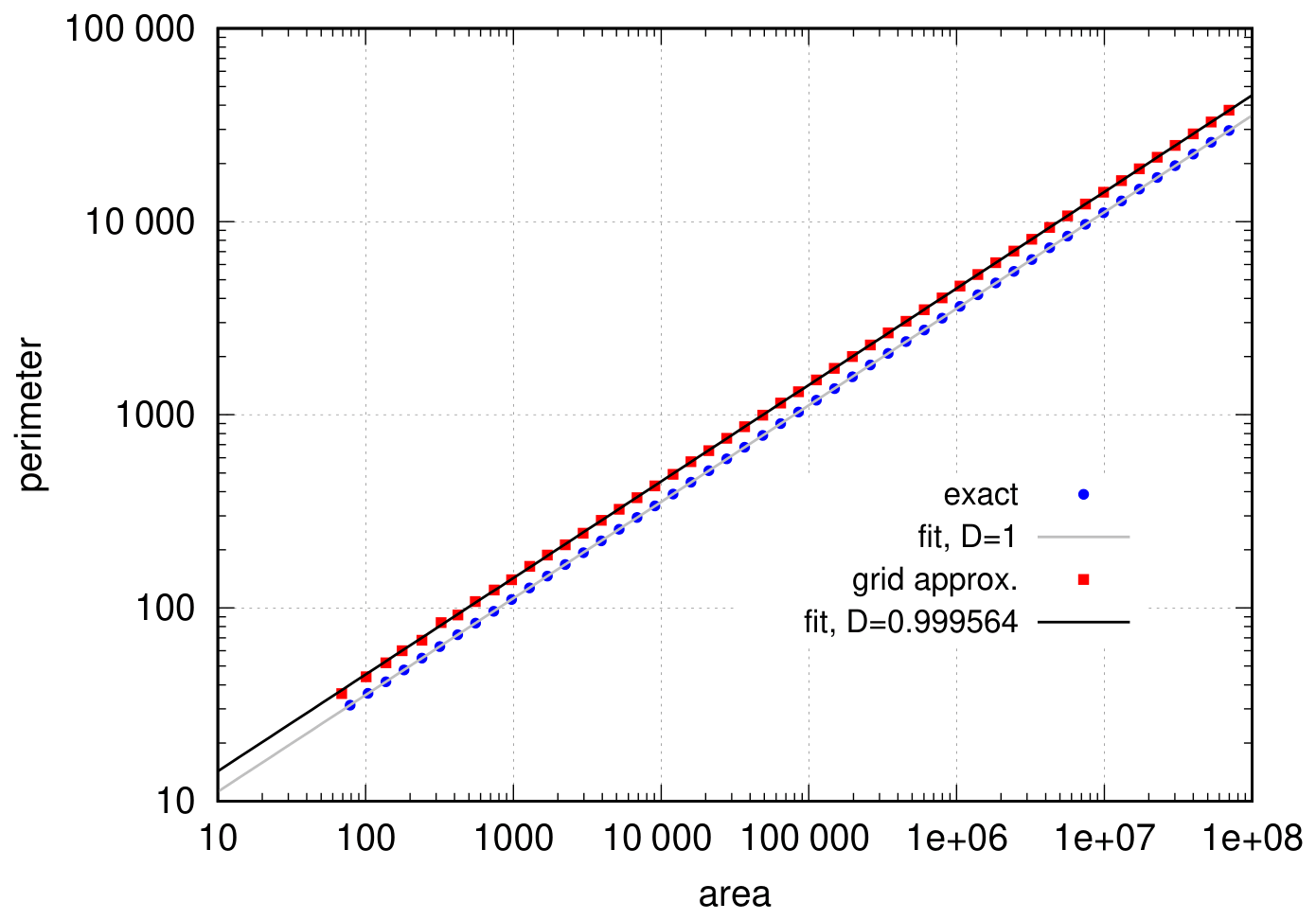
Figure C1 Systematic error for determining perimeters of spheres on gridded data. Blue circles indicate the exact values (with a fractal dimension D=1), red squares indicate the numerically derived values (with a fractal dimension D=0.999564). The dimensions were obtained using a linear regression to the data points in logarithmic scale.

Appendix D: Weibull plots

Here we give a short explanation for the use of the Weibull plot. The general form of a Weibull probability distribution of a non-negative random variable x is given by

$$\begin{array}{}\text{(D1)}& f\left(x\right)=\mathit{\gamma }p{x}^{p-\mathrm{1}}\exp (-\mathit{\gamma }{x}^p)\end{array}$$

with the shape parameter $p\in {\mathbb{R}}_{+}$, responsible for the slope of the distribution, and the scale parameter γ∈ℝ. The cumulative distribution (i.e. via integration) can be written as

$$\begin{array}{}\text{(D2)}& \begin{array}{rl}& F\left(x\right)=\underset{\mathrm{0}}{\overset{\mathrm{\infty }}{\int }}f\left(t\right)\mathrm{d}t=\mathrm{1}-\exp (-\mathit{\gamma }{x}^p),\\ & \text{i.e.}\mathrm{0}\le F\left(x\right)\le \mathrm{1}.\end{array}\end{array}$$

This equation can be reformulated as follows.

$$\begin{array}{ll}\text{(D3)}& {\displaystyle }\mathrm{1}-F\left(x\right)=\exp (-\mathit{\gamma }{x}^p)& {\displaystyle }\iff {\displaystyle \frac{\mathrm{1}}{\mathrm{1}-F\left(x\right)}}=\exp \left(\mathit{\gamma }{x}^p\right)\text{(D4)}& {\displaystyle }& {\displaystyle }\iff \log \left({\displaystyle \frac{\mathrm{1}}{\mathrm{1}-F\left(x\right)}}\right)=\mathit{\gamma }{x}^p{\displaystyle }& {\displaystyle }\iff \log \left(\log \left({\displaystyle \frac{\mathrm{1}}{\mathrm{1}-F\left(x\right)}}\right)\right)\\ \text{(D5)}& {\displaystyle }& {\displaystyle }=\log \left(\mathit{\gamma }{x}^p\right)\end{array}$$

Finally, we end with this equation

$$\begin{array}{}\text{(D6)}& \log \left(\log \left({\displaystyle \frac{\mathrm{1}}{\mathrm{1}-F\left(x\right)}}\right)\right)=\log \left(\mathit{\gamma }\right)+p\cdot \log \left(x\right)\end{array}$$

thus constituting a linear relationship between the quantities $\mathit{\eta }:=\log (-\log (\mathrm{1}-F\left(x\right)\left)\right)$ and ξ=log (x) with a slope of p. Thus, using a scatter plot of variables (ξ,η) we can derive the parameter p via linear regression.