Assessing combinations of regional MCB designed to target multiple climate response objectives

Marine Cloud Brightening (MCB) is a proposed method of Solar Radiation Modification (SRM). MCB proposes the injection of sea salt aerosols into marine clouds to enhance their reflectivity aiming to counteract greenhouse gas (GHG) driven warming. Modelling suggests that the climate effect of MCB depends on the location of deployments, with some regional MCB deployments resulting in potentially undesirable climate changes. MCB in midlatitude regions was found to cause a relatively homogeneous temperature and precipitation change pattern. Here we seek to quantify the trade-offs associated with different MCB strategies and to design an “optimal” deployment strategy. This study analyses 42 MCB patch simulations in UKESM1.0, spanning fourteen different regions and three different injection rates. These simulations are used to inform deployments with the aim to restore the SSP2-4.5 2040s mean climate to a baseline of 2014–2033. Multiple climate targets, consisting of global mean surface air temperature, precipitation, Arctic September sea ice extent, Southern Oscillation Index, and hemispheric mean temperatures, are used to inform the design of an optimised 14-region deployment and a reduced complexity optimised 6-region deployment, which we compare to the aforementioned midlatitude MCB deployment. Some improvements to the midlatitude MCB deployment are observed, in sea ice restoration and zonal mean temperature response. These results show it may be possible to design MCB strategies that target several climate responses simultaneously when combining regional MCB deployments. The results highlight the importance of including high latitude MCB to achieve Arctic sea ice restoration in UKESM1.0.

1 Introduction

Despite decarbonization efforts, the carbon dioxide (CO₂) emissions from fossil fuels and industry continue to rise, with record high greenhouse gas (GHG) emissions and human induced rates of global warming over the period 2014–2023 (Forster et al., 2025). There is an increasing body of research into solar radiation modification (SRM) methods, which are proposed technologies that aim to cool the planet by deliberately increasing the reflection of incoming solar radiation back out to space. The two most prominent SRM methods are Stratospheric Aerosol Injection (SAI; Crutzen, 2006; Kravitz et al., 2011; Visioni et al., 2023b) and Marine Cloud Brightening (MCB; Twomey, 1974; Latham, 1990; Latham et al., 2008). MCB is a proposal to inject sea salt aerosols (SSA) into marine clouds, with the intention of increasing the reflectivity of the clouds through the Twomey effect (Twomey, 1977) and the Albrecht effect (Albrecht, 1989). The SSA act as cloud condensation nuclei (CCN), increasing the cloud droplet number concentration (CDNC) and, in turn, the cloud albedo (Twomey or cloud albedo effect). The reduced size of the cloud droplets tends to suppress precipitation, increase dry air entrainment, and increase cloud droplet evaporation. These have complex effects on cloud liquid water content and lifetime (together called cloud adjustments) (Feingold et al., 2024). In ESMs, the net effect tends to reduce the sink of liquid water which may increase the lifetime and coverage of clouds (Albrecht effect – Albrecht, 1989). The SSA themselves also scatter solar radiation through the direct aerosol effect. This component is sometimes referred to as marine sky brightening (MSB) and can significantly contribute to the negative radiative forcing in MCB simulations (Ahlm et al., 2017; Feingold et al., 2024). For example, Partanen et al. (2012) found a 29 % direct effect component of the total radiative effect for a strategy seeding all ocean areas.

Previous research on MCB has primarily focused on regions with high susceptibility to CCN perturbations, targeting stratocumulus decks (Jones et al., 2009; Jones and Haywood, 2012; Haywood et al., 2023; Chen et al., 2025). These regions have high proportions of low-level clouds with low CDNC. While these regions exhibited a strong Twomey effect, there were some undesirable climate responses to deployments in these regions. For example, Jones et al. (2009) and Jones and Haywood (2012) showed that MCB in the stratocumulus deck off the west coast of southern Africa results in detrimental precipitation deficits in the Nordeste and Amazon regions of Brazil, a feature reproduced by multiple Earth System Models (ESMs) (Hirasawa et al., 2023; Rasch et al., 2024). Haywood et al. (2023) and Chen et al. (2025) showed that deploying solely in the susceptible regions of the East Pacific results in very strong La Niña-like responses. Additionally, Xing et al. (2025) found MCB in the subtropical eastern Pacific results in a mean-state La Niña tendency and suppresses ENSO variability, reducing ENSO amplitude by approximately 61 %.

The Geoengineering Model Intercomparison Project (GeoMIP) aims to coordinate geoengineering simulations to limit the differences in model setup to enable multi-model analyses (Kravitz et al., 2011; Visioni et al., 2023a). GeoMIP has conducted many SAI and MCB experiments. The G3 sea-salt climate engineering (G3-SSCE; Alterskjaer et al., 2013) experiment, was designed to simulate 50 years of MCB between 30° S and 30° N starting in 2020 to counteract the radiative forcing in the Representative Concentration Pathway 4.5 (RCP4.5), followed by 20 years where the MCB is stopped to investigate the termination effect. MCB has been simulated by prescribing increases to CDNC, as in the G4cdnc experiment (Kravitz et al., 2013; Stjern et al., 2018), as well as injection of SSA into the marine boundary layer, for example in G4sea-salt (Kravitz, 2013; Ahlm et al., 2017). These simulations showed more uniform cooling than targeting solely the subtropical stratocumulus decks, though there was still substantial residual cooling at high latitudes. Chen et al. (2024), more recently, focused on strategies targeting less susceptible regions which was found to provide a more uniform global cooling. The susceptibility of regions was estimated using the shortwave cloud forcing from an increase of in-cloud CDNC to 375 cm⁻³. These findings motivate further research into understudied regions. Rasch et al. (2024) analysed regional MCB in 6 marine regions (the Northern Ocean, South-East Atlantic, and North, North-East, South-East and South Pacific) across three ESMs. That work was extended in Hirasawa et al. (2026a) to include more regions or “patches”, along with a comparison of stratocumulus deck MCB in subtropical ocean regions to a midlatitude MCB strategy. This midlatitude strategy was shown to give a temperature and precipitation pattern which more closely resembles the opposite of GHG-driven changes relative to previously studied MCB strategies, though many residual regional climate changes remain.

MCB differs from SAI in the heterogeneity of its potential deployments. The aerosols in SAI deployments have a much longer residence time and quickly spread zonally in the stratosphere. In contrast, aerosols in MCB deployments have shorter lifetimes resulting in a more localized perturbation. This provides both challenges and opportunities when considering how different patches of MCB might be combined. Past GCM studies highlight the need to carefully consider the spatial distribution of MCB intervention, as the effect of MCB is strongly dependent on the location of the SSA emissions. While there are many approaches to designing SRM strategies and scenarios, such as targeting specific regional climate changes, here we aim to develop a strategy that simultaneously reduces GHG climate impacts by targeting multiple key climate metrics. Explicitly simulating all possible combinations of MCB deployments using ESMs is not feasible. However, with a much larger array of MCB simulations, further research into MCB deployment design is possible. The additional flexibility of MCB deployment design with respect to SAI highlights a need for research into optimization of MCB implementations that target multiple metrics from the climate response together. This study aims to work towards this research need, exploring the trade-offs and limits of potential MCB strategies. Akin to applications of Green's function methods to understanding climate responses (Liu et al., 2018; Bloch-Johnson et al., 2024; Kooloth et al., 2025), this study uses MCB simulations in different regions to estimate responses to a combined deployment in these various regions.

The paper is organized as follows. Section 2 provides a model description and outlines the base set of simulations. Section 3 examines the climate responses of this base set of simulations, extending the analysis of the 14 UKESM1.0 patch simulations considered in Hirasawa et al. (2026a), by investigating additional metrics and multiple injection rates. Section 4 describes the methodology used to produce two novel MCB scenarios from the patch simulations that are optimized to meet multiple climate metric targets. The climate responses to these novel MCB deployments are discussed in Sect. 5, with comparison to a midlatitude MCB deployment similar to the new G6-MCB-1.5K experiment strategy (Hirasawa et al., 2026b). Finally, Sect. 6 summarises and discusses the findings of this research.

2 Model description and outline of simulations

The simulations are run using the UK Earth System Model, UKESM1.0 (Sellar et al., 2019), which is a fully coupled ESM. The physical model uses HadGEM3-GC3.1, an atmosphere–land–ocean–sea ice model (Kuhlbrodt et al., 2018). This includes an atmosphere model with grid resolution of 1.875° in longitude, 1.25° in latitude and 85 model levels up to 85 km altitude (Walters et al., 2019). There is coupling to several Earth system components including ocean (Storkey et al., 2018), sea ice (Ridley et al., 2018), ocean biogeochemistry (Yool et al., 2013), land surface and vegetation (Best et al., 2011), and atmospheric chemistry (Archibald et al., 2020) from the United Kingdom Chemistry and Aerosol (UKCA) model (Morgenstern et al., 2009; O'Connor et al., 2014).

Coupled to the atmospheric chemistry is the UKCA two-moment modal aerosol microphysics scheme, called GLOMAP-mode. The GLOMAP-mode scheme (Mann et al., 2010) is used to represent aerosol mass and number for 4 aerosol species (sulfate, sea-salt, black carbon (BC), and organic carbon (OC)) as internal mixtures across five lognormal size modes. Dust is modelled separately by the Coupled Large-scale Aerosol Simulator for Studies in Climate (CLASSIC) bin scheme (Woodward, 2001). The aerosol activation scheme is based on the Abdul-Razzak and Ghan (2000) aerosol activation parameterisation to diagnose CDNC, described further by West et al. (2014). The RADAER scheme is used to simulate the direct radiative effect from aerosols using specific scattering and absorption coefficients, and the dimensionless asymmetry parameter of the aerosols, as described in Bellouin et al. (2013). For a full description of the aerosol scheme in HadGEM3-GC3.1 and UKESM1.0, and how the Earth system couplings in UKESM1.0 lead to differences between the two models, the reader is referred to Mulcahy et al. (2020).

Consistent with the G6MCB simulations outlined in Haywood et al. (2023), SSA injection is represented by enhancing the primary sea-salt emissions scheme. SSA are emitted into the lowest model level which is centred at approximately 20 m. Bins 1–12 of the 20-bin sea salt emissions scheme are mapped to the accumulation mode in GLOMAP-mode; SSA are emitted into bin 10, which has a mid-bin dry diameter of 172 nm. This aerosol size was chosen to maximise the cooling from MCB in UKESM1.0 for subtropical injection locations (Haywood et al., 2023). The SSA are injected into the open ocean parts of the regions outlined in Fig. 1 (grid cells with a land fraction equal to 0.0). Each region was selected to have similar open ocean areas for SSA injection.

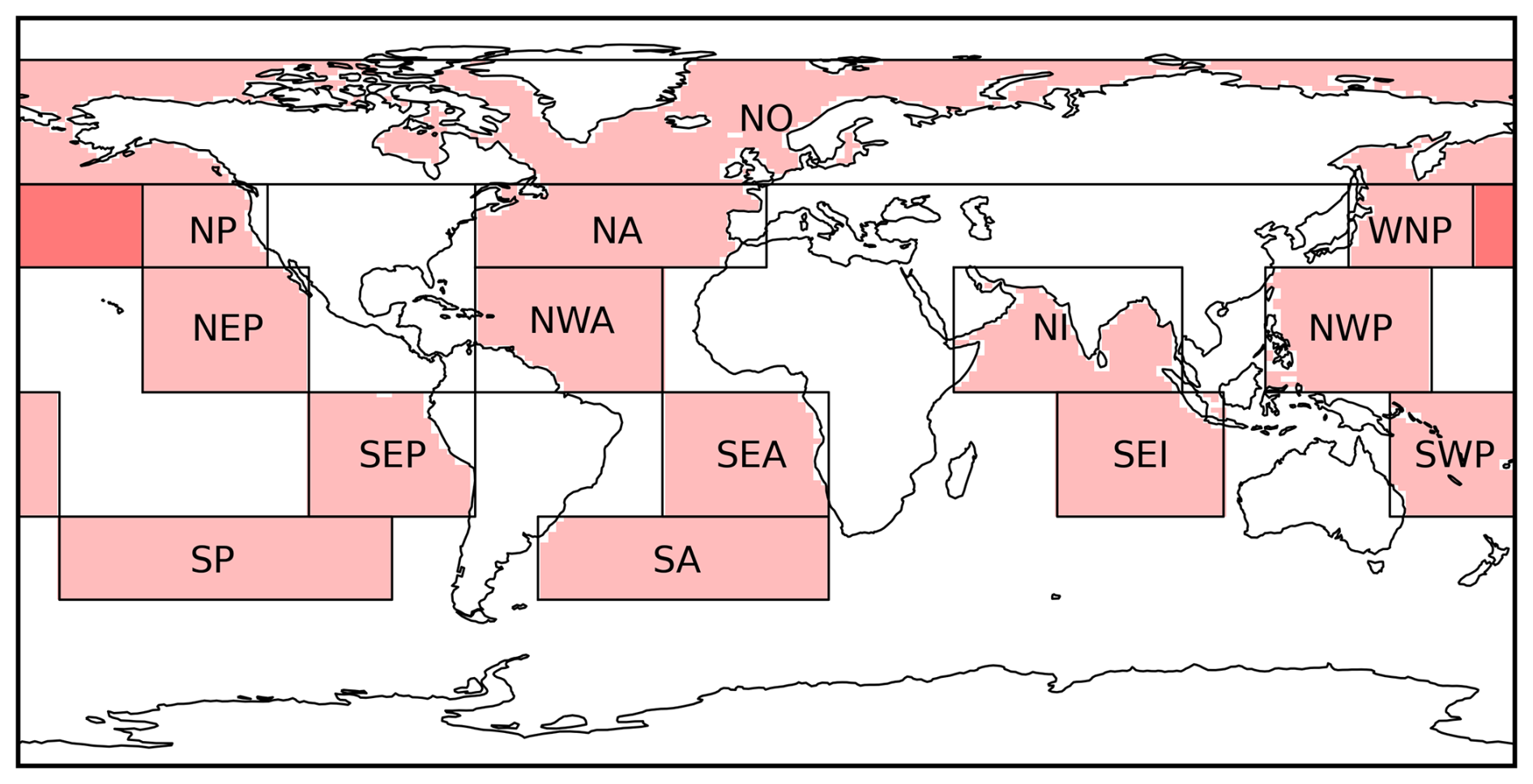
Figure 1 The locations of the 14 different regions where MCB is deployed in this study. The different regions are: Northern Ocean (NO), North Pacific (NP), North-East Pacific (NEP), South-East Pacific (SEP), South Pacific (SP), Western North Pacific (WNP), North-West Pacific (NWP), South-West Pacific (SWP), North Atlantic, (NA), North-West Atlantic (NWA), South-East Atlantic (SEA), South Atlantic (SA), Northern Indian (NI), and South-East Indian (SEI). The red shading shows the open ocean grid points of a given box, showing where SSA are emitted. Note that the WNP and NP regions overlap, illustrated by the darker shading, as outlined in Table 1.

Table 1 Definitions of the regions used in this study, as shown in Fig. 1. The open ocean area for the Northern Ocean (NO) is nominal owing to variable sea ice fraction.

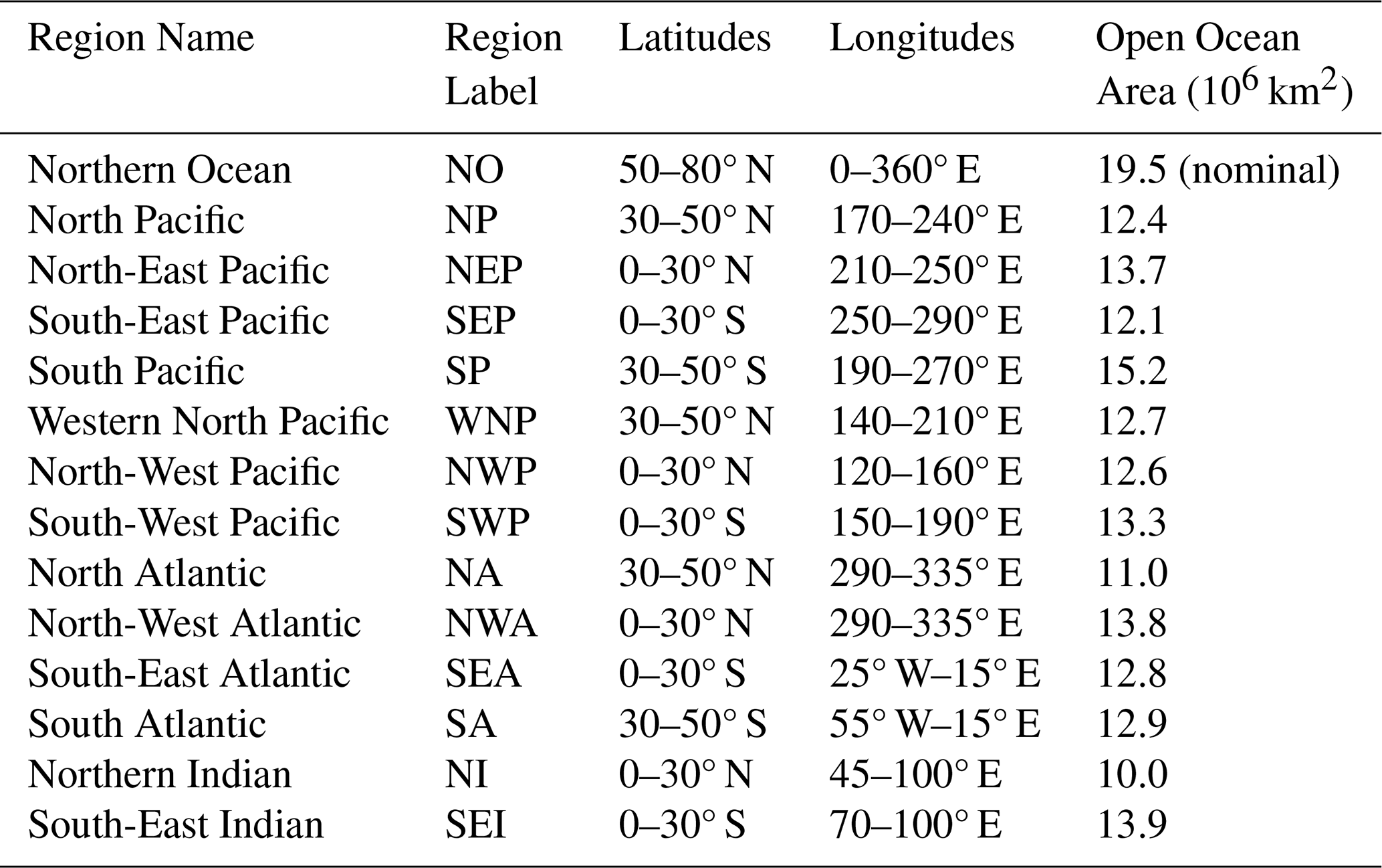
Table 1 lists the definitions of the 14 regions shown in Fig. 1. For each of these regions, pairs of coupled and prescribed sea surface temperature (SST) simulations are run for 3 different injection rates: 5, 10 and 50 Tg yr⁻¹. These are time-invariant emissions, applied continuously throughout the year, except for the Northern Ocean (NO) region. In the NO region, the 5, 10 and 50 Tg yr⁻¹ SSA emissions rates are nominal. The true emission rate is scaled by the sea ice free fraction of a given grid cell, which results in a seasonal variation of SSA emission rates, along with slight annual variation due to the seasonal and inter-annual variability in sea ice coverage, as discussed in Henry et al. (2025). The SSA emission reach their annual maximum when the sea ice area is at its minimum in September, when the emission rate is approximately 1.5 times the minimum emission rate (typically in March) for a given injection rate. The fixed SST simulations are 10-year transient Atmospheric Model Intercomparison Project (AMIP) simulations from 1979 to 1989 (Eyring et al., 2016) used to calculate the effective radiative forcing (ERF) of the different regional MCB deployments; this is examined in Sect. 3.1. The fully coupled simulations are based on a medium emissions scenario, the Shared Socioeconomic Pathway 2-4.5 (SSP2-4.5; Fricko et al., 2017), and run for 15 years from 2035, averaging the results over the final 10 years. Four additional simulations, where 2.5, 5, 10 and 50 Tg yr⁻¹ of SSA are injected into all 14 regions at once, totalling 35, 70, 140 and 700 Tg yr⁻¹ respectively, are run to inform the methodology to produce optimised MCB deployments and to investigate how additive the regional MCB deployments are. Finally, three 50 Tg yr⁻¹ coupled simulations are run for 15 years from 2035, comparing two optimised MCB deployments to a midlatitude deployment. These deployments are discussed further in Sect. 4.2. The Unified Model (UM) version used in this study is no longer supported, preventing an expansion in ensemble size for these three simulations with the same configuration. A single ensemble member is, therefore, a limitation of this study. However, an exploration of the climate responses of these simulations in Sect. 5 act as a proof of concept for the methodology used in this paper. Future studies should certainly expand on the ensemble size.

3 Forcings and Climate Responses from the Base Set of simulations

3.1 AMIP simulations

Figure 2a illustrates the ERF from the base set of 42 simulations used in this study, along with the contributions from the cloud radiative forcing (CRF) in Fig. 2b and the direct radiative forcing (DRF) in Fig. 2c, relative to the control simulation (Ghan, 2013). These latter components correspond to the indirect and direct effect contributions to the ERF, respectively, although some of the CRF may also be driven by dynamical responses. Residual differences between the total ERF and the sum of the CRF and DRF may be attributed to surface albedo changes and/or atmospheric rapid adjustments (Smith et al., 2018, Weber et al., 2024). The bar charts are sorted by the magnitude of the total ERF to the 50 Tg yr⁻¹ simulations of a given region.

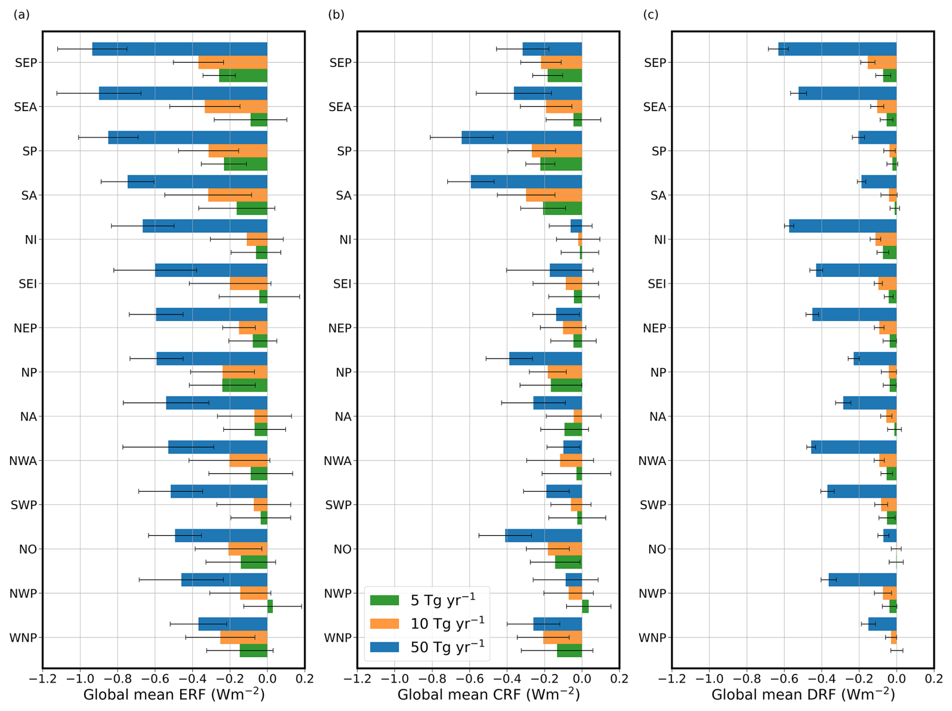
Figure 2 Panel (a) shows the 10-year mean ERF from the MCB simulations for the different regions shown in Fig. 1 and defined in Table 1. The cloudy and clear-sky components of the ERF are shown in panels (b) and (c) respectively. Error bars show one standard deviation of the annual mean ERF responses.

Areas with major stratocumulus decks which are susceptible to the addition of aerosols (e.g. SEP, SEA, NEP) show strong radiative forcing response to SSA, which supports the choice of these areas for injection in earlier studies (e.g. Jones et al., 2009; Haywood et al., 2023). The SEA and SEP give the most negative ERF for the 50 Tg yr⁻¹ injection rate, whereas the NEP ERF for this injection rate is approximately a third weaker. Previous studies found that the NEP region has both less climatological low cloud cover and smaller increases in cloud cover relative to SEP and SEA in UKESM1, which causes the area-averaged ERF susceptibility (Rasch et al., 2024; Hirasawa et al., 2026a). Figure 2b shows it is the SP and SA regions that have the largest contributions from the CRF at all three injection rates, similar to two other ESMs (Hirasawa et al., 2026a). However, SEP and SEA have larger total ERF because stronger insolation at lower latitudes results in larger DRF in these regions. The SP and SA regions have lower background CDNC and higher liquid water path (LWP) compared to SEA and SEP as shown in Fig. S1 in the Supplement. While MCB in these regions results in a similar absolute change in CDNC in these regions, the higher background CDNC in the SEA and SEP show these regions are initially more saturated with aerosol particles. Therefore, the addition of aerosols to the SP and SA seeds clouds whereas the SEP and SEA are already cloudy and saturated with aerosols, so the additional aerosols are directly scattering sunlight rather than forming clouds. As the injection rate increases from 5 to 10 to 50 Tg yr⁻¹, the increase in CRF per additional Tg yr⁻¹ reduces, driving the “diminishing returns” in most areas investigated, with the ERF per Tg yr⁻¹ injection decreasing with increasing injection rate (Haywood et al., 2023). The ERFs of the 50 Tg yr⁻¹ injections are generally less than five times the 10 Tg yr⁻¹ simulations, with the DRF becoming an increasingly important component of the ERF for these high injection rates as shown by Fig. 2c.

3.2 Coupled simulations

Figures 3 and 4 show the pattern of the surface air temperature anomaly (ΔT) and precipitation anomaly (ΔP) in response to 50 Tg yr⁻¹ SSA injection for each of the 14 regions in the 2040s relative to SSP2-4.5. The pattern of responses varies greatly with the injection region. The global mean surface air temperature responses (ΔT_glob) for the 2040s vary up to a factor of three for the 50 Tg yr⁻¹ injections, with −0.13 °C for an NWA deployment compared to −0.56 °C for NP. Global mean precipitation responses (ΔP_glob) for the 2040s also vary up to a factor of three between deployment regions (e.g., SEP vs. NWP). The SEA precipitation response, in Fig. 4j, shows significant drying of the Amazon consistent with previous research (Jones et al., 2009; Jones and Haywood, 2012; Haywood et al., 2023; Rasch et al., 2024; Chen et al., 2025).

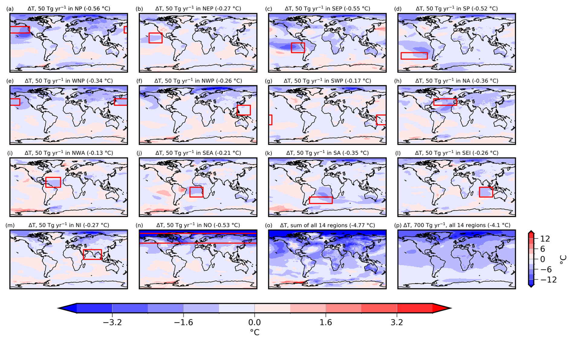
Figure 3 Panels (a–n) show the 2040s surface air temperature anomaly (ΔT) from the 50 Tg yr⁻¹ patch simulations relative to SSP2-4.5. Panel (o) shows the sum of the 14 responses in panels (a–n), for comparison with the 700 Tg yr⁻¹ simulation in panel (p). The 2040s global mean surface air temperature anomaly (ΔT_glob) is annotated in brackets above each panel. The horizontal colour bar corresponds to panels (a–n), and the vertical colour bar next to panel (p) corresponds to panels (o) and (p).

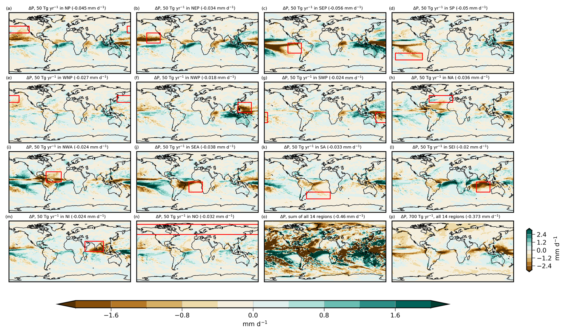
Figure 4 Same as in Fig. 3, but for 2040s precipitation anomaly (ΔP). The 2040s global mean precipitation anomaly (ΔP_glob) is annotated in brackets above each panel.

A comparison of the sum of these 14 simulations to the explicit 700 Tg yr⁻¹ simulation, where 50 Tg yr⁻¹ is deployed in each region simultaneously, is also shown in Fig. 3o and p and Fig. 4o and p. A cooling of 4.77±0.61 °C and a drying of 0.46±0.08 mm d⁻¹ from summing the individual responses compares to a cooling of 4.10±0.69 °C and a drying of 0.37±0.05 mm d⁻¹ responses for the 700 Tg yr⁻¹ simulation. ΔT_glob and ΔP_glob of the 700 Tg yr⁻¹ simulation reached 86 % and 80 % of the magnitude of the sum of all 14 responses in the 50 Tg yr⁻¹ patch simulations. The global mean ERF of the simulated 700 Tg yr⁻¹ simulation was 90 % of the sum of all 14 simulations. This non-additivity is consistent with previous studies which found the sum of responses to regional MCB perturbations tends to overestimate the cooling when MCB is applied simultaneously (Hill and Ming, 2012; Rasch et al., 2024; Hirasawa et al., 2026a). Hill and Ming (2012) identified a 19 % greater cooling from the sum of the temperature responses of three subtropical MCB regions compared to simulations of MCB in all three regions simultaneously, while Hirasawa et al. (2026a) found that the sum of cooling from five midlatitude regions overestimates cooling by 13 %–29 % in three models. Thus, models consistently indicate there is some non-linearity in the climate response to MCB. In terms of precipitation, Fig. 4o and p show much worse spatial agreement between the sum and explicitly simulated simulation for precipitation, in large part because it is a noisier field. Despite this limited spatial agreement, we assume that the global mean responses ΔP_glob are sufficiently additive, since the sum of the fourteen regional ΔP_glob anomalies is 80 % of the ΔP_glob response in the simultaneous 700 Tg yr⁻¹ emission simulation. As we shall see, when running strategies that include perturbations from many different areas simultaneously, the resulting zonal precipitation patterns show reasonable agreement with the desired target (Fig. 15) suggesting that the approach is valid.

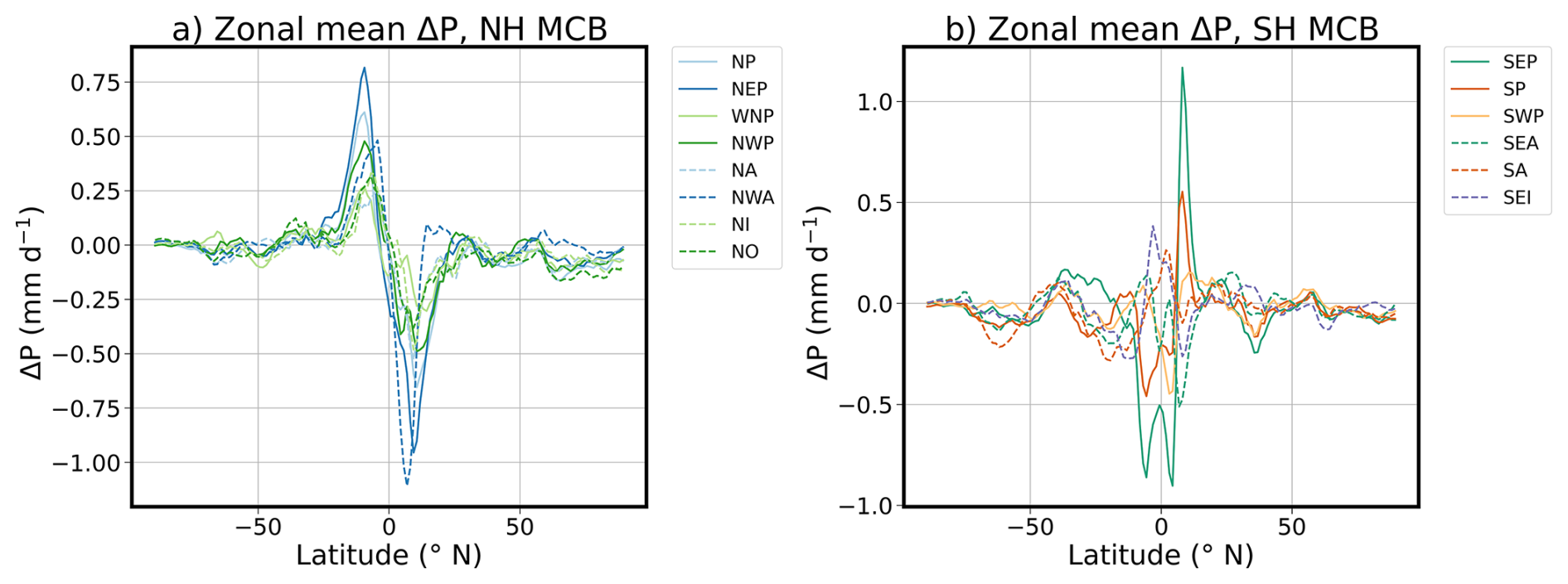
Figure 5 Zonal mean 2040s precipitation anomaly (ΔP) for the 50 Tg yr⁻¹ patch simulations in (a) the Northern Hemisphere (NH) and (b) the Southern Hemisphere (SH) relative to SSP2-4.5.

Analysis of the zonal mean ΔP shows a clear southward shift in the Intertropical Convergence Zone (ITCZ) for the Northern Hemisphere (NH) deployments, as shown by Fig. 5a. This is a feature shown in the shifting precipitation patterns in several of the maps in Fig. 4. For the Southern Hemisphere (SH) deployments, we also see changes in the ITCZ position but the trend is not as clear as for the NH deployments. The fact that NH MCB deployments lead to a southern shift of the ITCZ is consistent with NH SAI (e.g., Haywood et al., 2013), and have led to SAI design strategies that attempt to avoid perturbing the inter-hemispheric temperature balance to minimize impacts on the ITCZ (e.g. Kravitz et al., 2017). Design of an MCB combination strategy should therefore avoid seeding just the NH to avoid shifting the ITCZ southwards which could impact vulnerable regions such as South Asia and the Sahel.

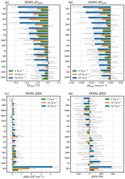
2040s mean climate responses of the 42 patch simulations for ΔT_glob, ΔP_glob, Southern Oscillation Index (ΔSOI) and Arctic September sea ice extent (ΔSSI) are summarized in Fig. 6a–d. Error bars show some of the temporal variability of the responses, spanning ± one standard deviation of the annual mean responses that make up the decadal mean responses plotted. These climate responses are analysed to inform the targets used in the methodology outlined in Sect. 4. ΔT_glob, ΔP_glob, ΔSOI and ΔSSI, as well as Northern Hemisphere and Southern Hemisphere mean temperature responses (ΔT_NH and ΔT_SH respectively), are chosen as targets. ΔT_glob, ΔP_glob and ΔSSI are targets consistent with previous SRM studies (Lee et al., 2020). The inclusion of ΔT_NH and ΔT_SH targets aims to avoid a hemispheric asymmetry in the cooling with respect to the target. To investigate the potential impacts of different patches on El Niño Southern Oscillation (ENSO), the mean sea level pressure difference between Tahiti and Darwin is used here as a simple measure of the SOI (Haywood et al., 2023). SOI is an oscillatory variable, so targets quantifying impacts on the magnitude and frequency of ENSO would be preferable for MCB optimisation. However, given our coupled simulation length of 15 years this analysis is not feasible. Instead, a mean ΔSOI target is included to prevent significant shifts to the SOI mean state and to avoid selecting MCB strategies that lead to large La Nina-like responses (Haywood et al., 2023; Chen et al., 2025). Other climate responses could have been chosen, but these were selected in this proof-of-concept study. They serve to illustrate how a proposed MCB deployment might incorporate targets into its design. However, any proposed MCB deployment would require very careful consideration of what targets to include or omit.

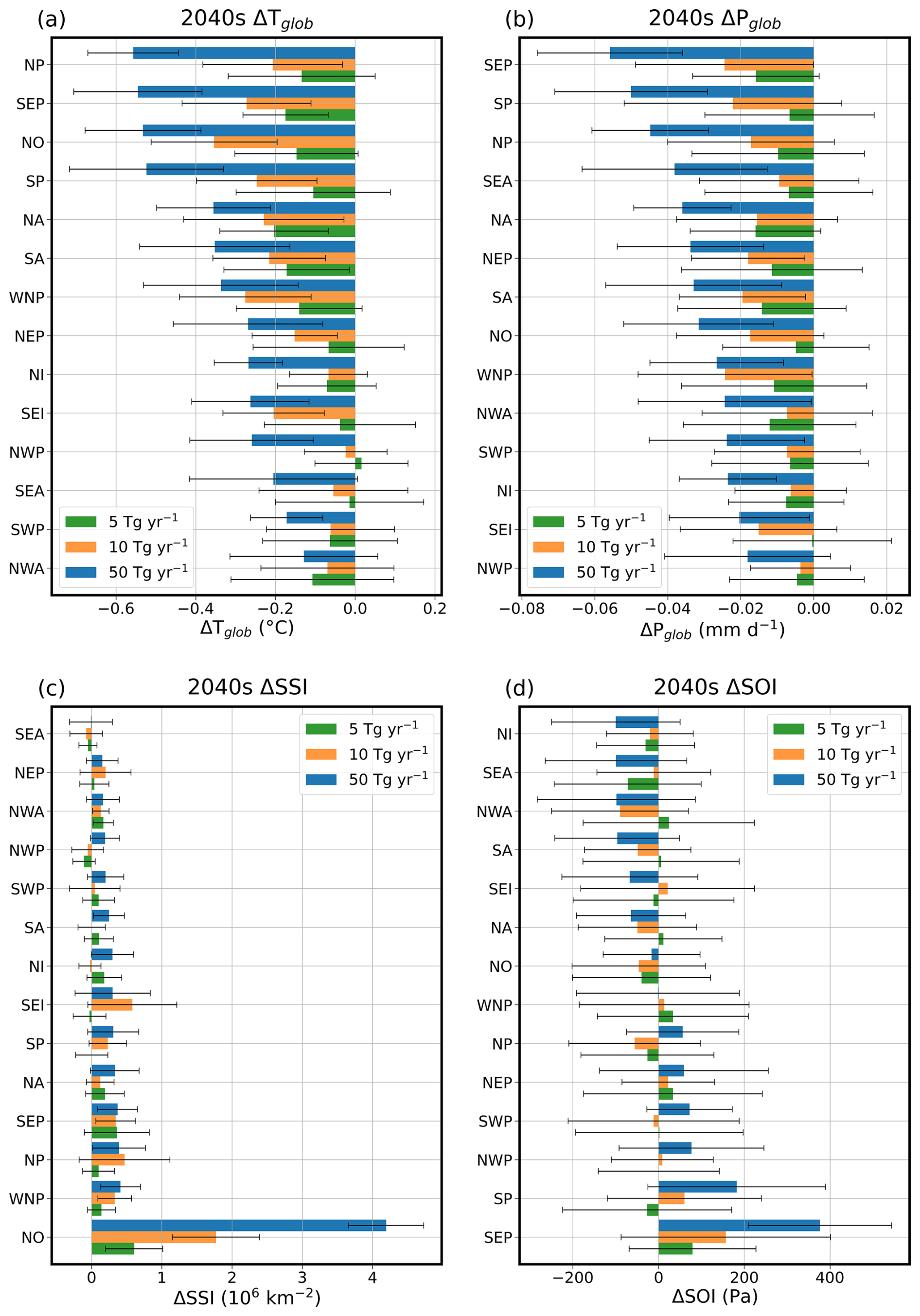
Figure 6 The 2040s mean responses of the patch simulations for global mean surface air temperature anomaly (ΔT_glob), global mean precipitation anomaly (ΔP_glob), Arctic September sea ice extent anomaly (ΔSSI) and Southern Oscillation Index anomaly (ΔSOI) are shown in panels (a)–(d) respectively. The 5, 10 and 50 Tg yr⁻¹ responses are shown as green, orange and blue bars respectively. Error bars show one standard deviation of the annual mean responses.

It is unsurprising that the largest sea ice restoration is seen in the NO patch, as this provides SSA and cooling closest to the sea ice (Henry et al., 2025). Figure 6c shows that most of the regions have an insignificant SSI response. MCB in the SEP region exhibited the largest impact on SOI, as shown in Fig. 6d, with the only statistically significant SOI response of all the patch simulations for SEP at 50 Tg yr⁻¹ SSA emission rate. This suggests that ENSO is most sensitive to seeding in the SEP region, with a positive SOI response of 377 Pa for a 50 Tg yr⁻¹ injection, making a La Niña state more likely. We note that studies using other fully coupled models have highlighted the strong La Niña response to aerosol radiative perturbations over the SEP region (Fasullo et al., 2024).

Figure 6a–d clearly show that between zero and 50 Tg yr⁻¹ injection rates there is non-linearity in the global mean coupled responses that varies from region to region. Incorporating information from simulations of lower injection rates is therefore critical to reduce uncertainty in estimates of responses to smaller injection rates. These coupled responses show larger variability, especially apparent in the ΔSOI responses in Fig. 6d. To reduce this variability, ideally an ensemble of simulations for each region and injection rate would need to be run. However, this would require another 84×15 year coupled simulations to produce three member ensembles. With comparison to the ERF responses in Fig. 2, it can be noted that the ERF variability is more constrained. Hence, in the absence of multiple coupled ensemble members for each patch simulation, this lower variability in the ERF responses is incorporated into the MCB deployment design methodology for combining the patch simulations to overcome the high variability of the coupled responses, as outlined in Sect. 4.

4 Methodology for designing MCB deployments from the base set of simulations

4.1 Defining climate response targets and sampling the combination space

There are an infinite number of possible MCB deployments that could be simulated. However, resources are limited and so it is important to narrow down to a handful of combinations. A target climate must first be defined to inform the deployment design and in order to narrow down the possible combinations. Any “optimised” deployment will depend greatly on these definitions of targets. The 2014–2033 mean climate is chosen here as this is the period in which the global mean temperature is 1.5 °C above preindustrial in SSP2-4.5 in UKESM1.0, consistent with previous studies (Henry et al., 2023).The aim here is the restoration of the 2040s mean climate in SSP2-4.5 to the 2014–2033 target climate with “optimised” MCB deployment. The targets are visualized in Fig. 7.

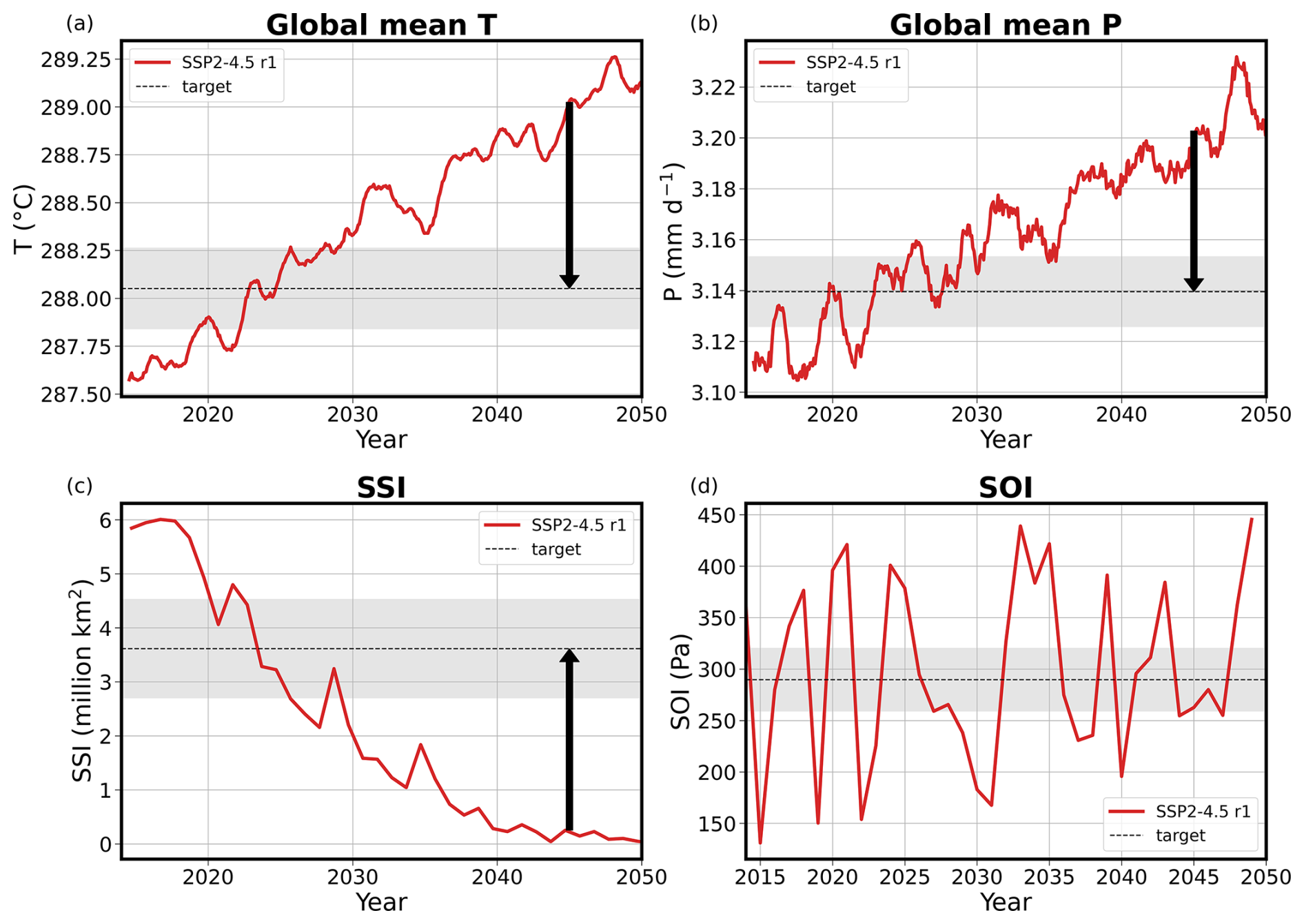
Figure 7 (a) Global mean surface air temperature, (b) global mean precipitation, (c) Arctic September sea ice extent (SSI) and (d) Southern Oscillation Index (SOI) targets, aiming to restore the 2040s climate to the 2014–2033 mean state (dashed line). The shading shows the target range and the black arrows show the magnitude for a conceptual target restoration. This is omitted in panel (d) due to the small magnitude of the SOI target.

Figure 8 illustrates linear interpolation of the ΔT_glob responses to the 35, 70 and 140 Tg yr⁻¹ MCB simulations spread evenly across all 14 regions. This suggests a 46 Tg yr⁻¹ equivalent simulation would restore the 2014–2033 ΔT_glob. Hence, in this study, we decide to sample combinations totalling 50 Tg yr⁻¹.

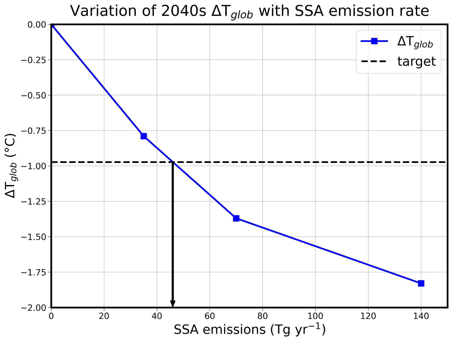
Figure 8 Variation of 2040s global mean surface air temperature anomaly (ΔT_glob) with sea salt aerosol (SSA) emission rate for a 35, 70 and 140 Tg yr⁻¹ MCB deployment with the SSA shared equally across the 14 regions. The dashed line indicates the target cooling required to restore the 2014–2033 ΔT_glob. Linear interpolation suggests a 46 Tg yr⁻¹ is required to achieve this cooling target.

The base set of 42 simulations are used to estimate the climate responses from a given combination of regions and SSA injection rates. Putting n identical objects into k boxes results in $\left(\begin{array}{c}n+k-\mathrm{1}\\ n\end{array}\right)$ distinct combinations. Here, the possible combination space is spanned by considering a 50 Tg yr⁻¹ deployment shared in multiples of 5 Tg yr⁻¹ across the 14 regions. This can be thought of as putting 10 identical 5 Tg yr⁻¹ shares into any of the 14 regions, giving a total of $\left(\begin{array}{c}\mathrm{10}+\mathrm{14}-\mathrm{1}\\ \mathrm{10}\end{array}\right)=\mathrm{1}\mathrm{144}\mathrm{066}$ distinct combinations. This choice balances the computational constraint of handling a large number of combinations. Using multiples of 5 Tg yr⁻¹ shares allows the responses from the 5, 10 and 50 Tg yr⁻¹ base simulations to be used directly, with interpolation only necessary for values between 10 and 50 Tg yr⁻¹. The total emission constraint of a combination is described by Eq. (1):

$$\begin{array}{}\text{(1)}& {\sum }_{i=\mathrm{1}}^{N=\mathrm{14}}{x}_i=\mathrm{50}\mathrm{Tg}{\mathrm{yr}}^{-\mathrm{1}}\end{array}$$

where x_i is the mass of SSA in Tg yr⁻¹ injected into the region i for a given MCB combination, taking values of 0, 5, 10… up to 50 Tg yr⁻¹.

Additivity and linearity of the responses from the base set of simulations is assumed. There is significant variability in the coupled responses particularly for the 5 and 10 Tg yr⁻¹ simulations. Relying on the coupled responses alone failed to achieve the desired climate targets. To overcome the variability, this methodology uses the more constrained ERF to scale down the 50 Tg yr⁻¹ coupled responses. In this analysis, the estimated climate response, R, from a given combination is approximated as the sum of the ERF-weighted climate response from the patch simulations of the 14 regions, outlined in Eq. (2):

$$\begin{array}{}\text{(2)}& R={\sum }_{i=\mathrm{1}}^{N=\mathrm{14}}{\displaystyle \frac{{\text{ERF}}_i\left(x_i\right)}{{\text{ERF}}_i\left(\mathrm{50}\mathrm{Tg}{\mathrm{yr}}^{-\mathrm{1}}\right)}}\times r_i\left(\mathrm{50}\mathrm{Tg}{\mathrm{yr}}^{-\mathrm{1}}\right)\end{array}$$

where ERF_i(x_i) and ERF_i(50 Tg yr⁻¹) are the ERF to SSA injection in region i at x_i and 50 Tg yr⁻¹ emission rates respectively, and r_i (50 Tg yr⁻¹) is the climate response to a 50 Tg yr⁻¹ deployment in region i. Therefore, this directly uses the ERF data from the 5, 10 and 50 Tg yr⁻¹ prescribed SST simulations, and interpolates the ERF for values between 10 and 50 Tg yr⁻¹. The 50 Tg yr⁻¹ coupled responses themselves have high variability. However, owing to the larger rate of SSA emission they have higher signal-to-noise ratios, and the variability is less significant compared to the absolute mean coupled response than for the 5 and 10 Tg yr⁻¹ simulations. Thus, we focus on using 50 Tg yr⁻¹ as a pragmatic decision, made in the absence of many ensemble members and longer simulations that might otherwise reduce the uncertainty in the 5 and 10 Tg yr⁻¹ coupled responses.

This method provides an initial prediction of the climate responses from a given combination and allows the visualisation of different parameter spaces spanned by the sample of over a million combinations. This is illustrated for the ΔT_glob and ΔP_glob response parameter space in Fig. 9, which shows that combinations with the largest cooling tend to give the largest drying, a trend expected from the relationship of global mean precipitation with global mean temperature consistent with the Clausius–Clapeyron equation (Trenberth et al., 2003). These parameter spaces can be used to investigate how multiple climate response targets could be met simultaneously with a single combination of patch simulations.

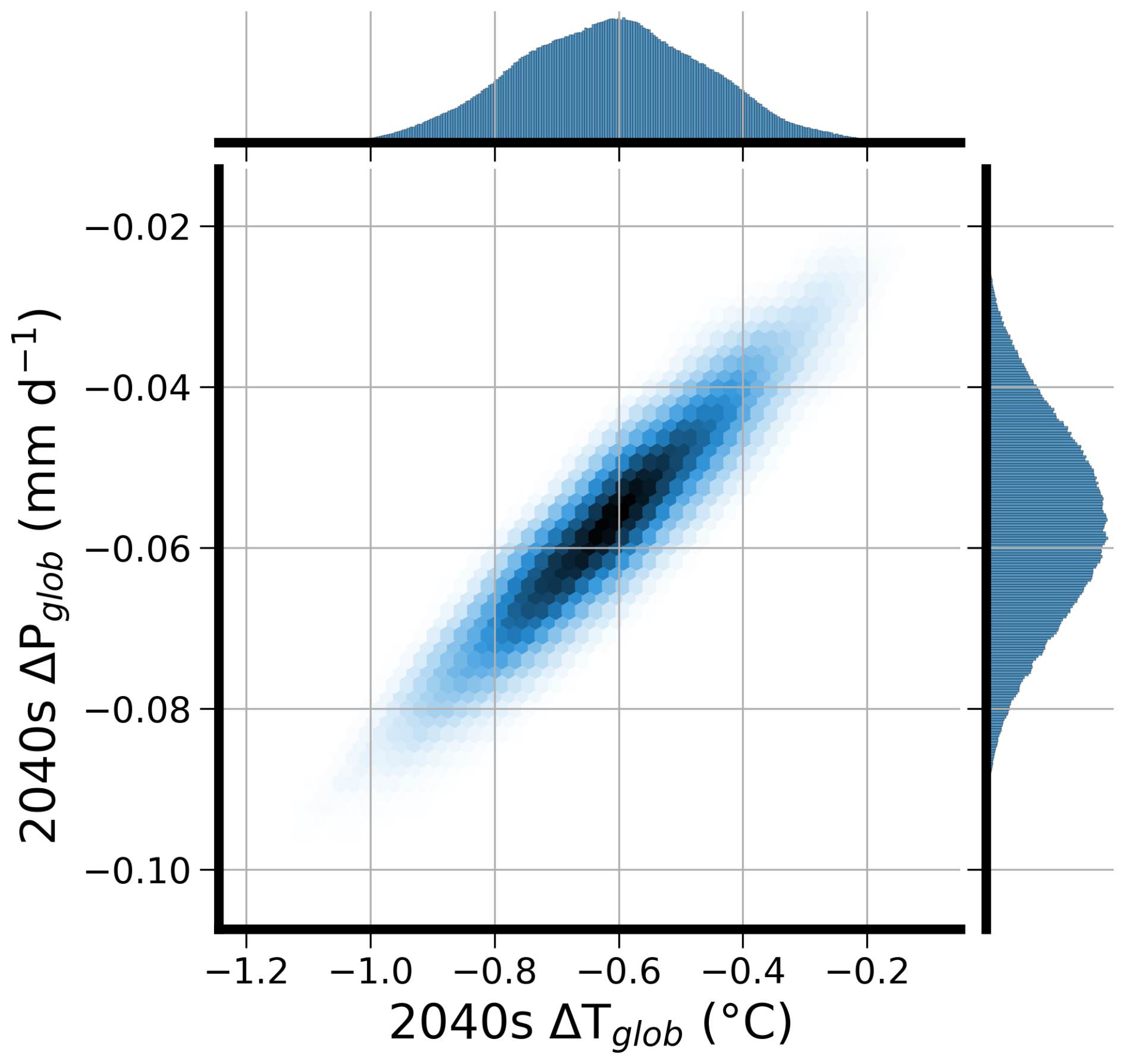
Figure 9 A heatmap of the 2040s global mean precipitation anomaly (ΔP_glob) against 2040s global mean surface air temperature anomaly (ΔT_glob) combination space for a 1 144 066 sample of possible 50 Tg yr⁻¹ MCB combinations, estimated using Eq. (2), assuming additivity and linearity with the patch simulations.

4.2 Filtering the combination space

The target ranges and filtering process are summarized in Table 2 and Fig. 10. The difference between the 2014–2033 mean responses for SSP2-4.5 and the 2040s mean for the control run of these MCB simulations are listed in the target column of Table 2. The autocorrelated standard deviation of the annual mean coupled responses for the 2014–2033 baseline and 2040s control run is used as the tolerance for a given target, providing a target range. Any combination that has a response that falls outside a target range is excluded. The application of ΔT_glob, ΔP_glob, ΔSOI, ΔSSI, ΔT_NH and ΔT_SH targets restricts the number of possible combinations to 172 (Table 2). Figure 10 visualizes this process of narrowing down the combination space to a sample which satisfy all of these specified climate response targets. The different coloured lines in the first column of plots correspond to the target ranges used for each filtering step.

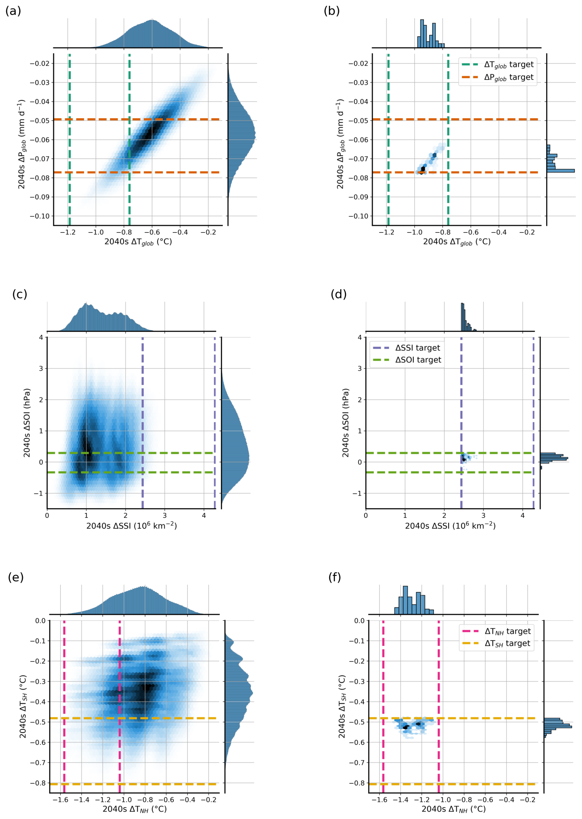
Figure 10 Heatmaps showing the narrowing down of the combinations based on climate response targets defined in Table 2. Panels (a), (c) and (e) show the heatmaps for the 1 144 066 combinations. Panels (b), (d) and (f) show the heatmaps for the remaining 172 combinations that satisfy all 6 climate response targets. Dashed lines show the upper and lower bounds of a given target.

Table 2 Climate response targets.

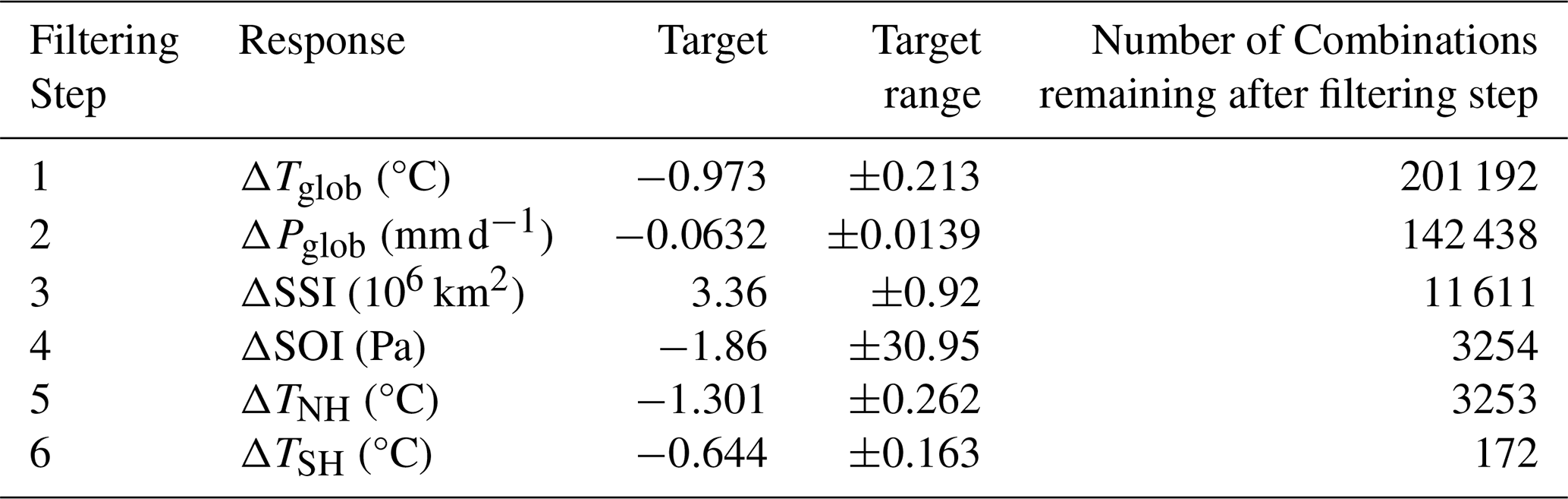
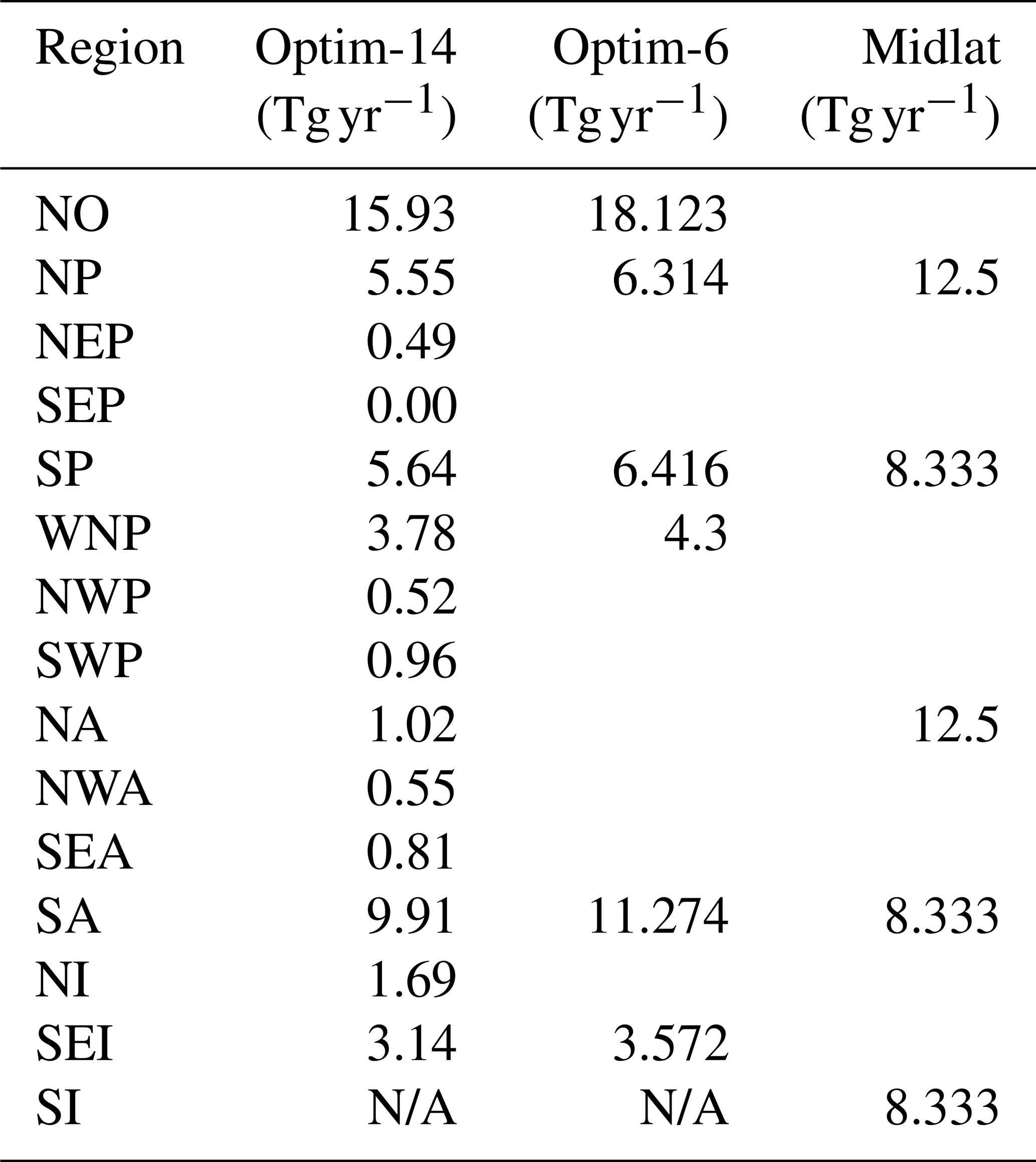
There are 172 of the 1 144 066 combinations that satisfy all 6 targets simultaneously. The average of these remaining 172 combinations is used to provide the distribution of the 50 Tg yr⁻¹ deployments across the 14 regions for a novel MCB deployment optimized for the climate response targets. This deployment is named “Optim-14”. An additional simulation, “Optim-6”, is run where the 6 most significant regions of Optim-14 are chosen, and the injection rates are rescaled to a total of 50 Tg yr⁻¹. The basis for reducing the regions of the deployment from 14 to 6 is pragmatic. Any practical deployment would seek to reduce the number of deployment areas to as few as practically possible. We choose 6 as this is a similar number to the 5 areas used in Hirasawa et al. (2026a). Hirasawa et al. (2026a) suggests that a midlatitude deployment of MCB would lead to a pattern of cooling which is similar to the warming from increased GHGs relative to previously studied MCB strategies. Therefore, a midlatitude deployment is also simulated for comparison with the novel MCB deployments, named “Midlat”. These three deployments are summarised in Table 3 and visualized in Fig. 11a–c, and the climate responses from these deployments are the subject of the next section. It is important to note the Midlat deployment involves injection into an additional region, the South Indian (SI) region, which is not considered in the methodology used in this paper. The SI region spans 30–50° S in latitude and 30–100° E in longitude, and is included in the Fig. 11c visualization of the Midlat deployment.

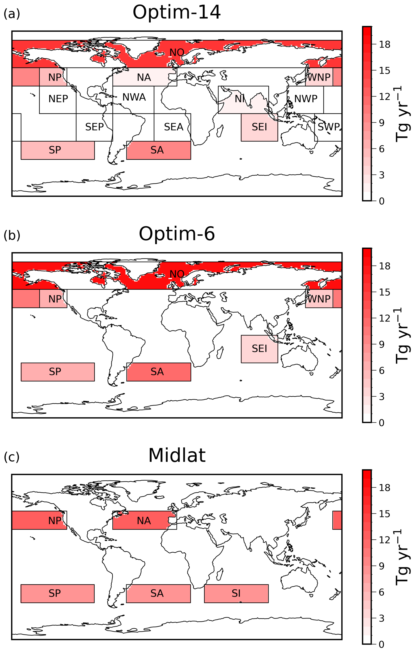
Figure 11 The distribution of the 50 Tg yr⁻¹ deployments for (a) Optim-14, (b) Optim-6 and (c) Midlat.

Table 3 Injection rates and locations for the Optim-14, Optim-6 and Midlat deployments.

The choice of metrics influences the optimisation; therefore, this methodology could be extended to incorporate other climate response targets that would further restrict the 172 combinations. For example, an optimised deployment could consider impacts on the position of the ITCZ, along with other climate response considerations. Although an ITCZ target was not incorporated in the optimisation in this study, impacts of the optimised MCB deployments on the ITCZ are considered in Sect. 5.

5 Analysis of novel MCB deployments

5.1 Assessments of the optimised deployments with respect to a midlatitude MCB deployment

Figure 12 compares the restoration of target temperature and precipitation responses for Optim-14, Optim-6 and Midlat. The correlation scores show some improvement relative to the midlatitude deployment for temperature both globally and over land, with more modest improvements in the precipitation correlation scores. There is some statistically significant residual warming in South America for all three deployments, but with a greater magnitude for Optim-14 and Optim-6. This was not specifically targeted in the design of these three deployments, but perhaps an improved deployment would address this as a target to avoid this residual warming. All three deployments exhibit statistically significant overcooling with respect to the target in ocean regions. These unsurprisingly are apparent in the regions where most SSA are emitted in the model, for example, in the NO region for both Optim-14 and Optim-6, and the SA and SP regions for all three strategies.

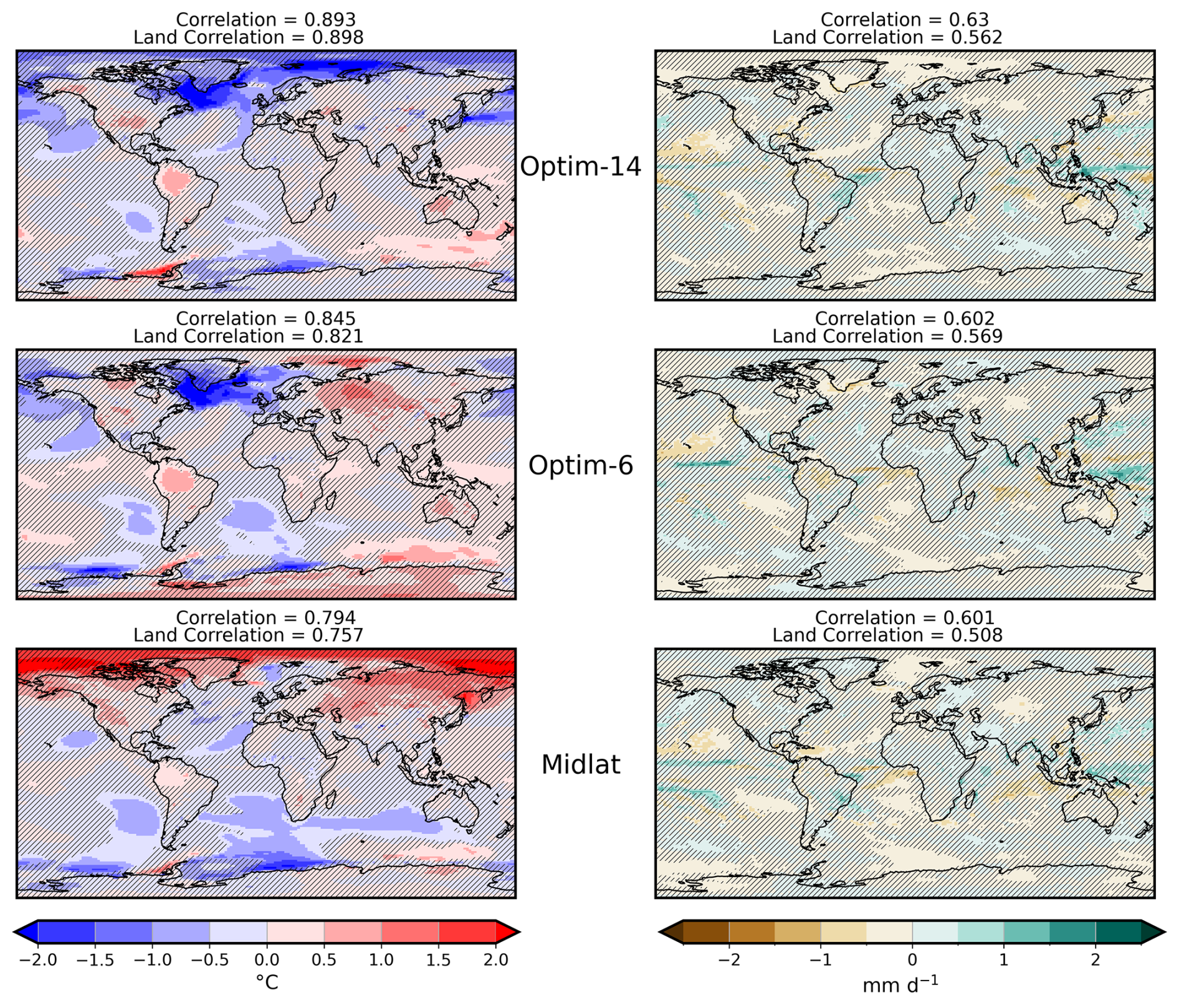
Figure 12 Difference in temperature and precipitation 2040s mean responses of Optim-14, Optim-6 and Midlat from the 2014–2033 target. Area-weighted spatial Pearson correlation scores, calculated both globally and over land, are annotated, with hatching showing non-significant grid points at the p<0.05 level using a Student's t-test.

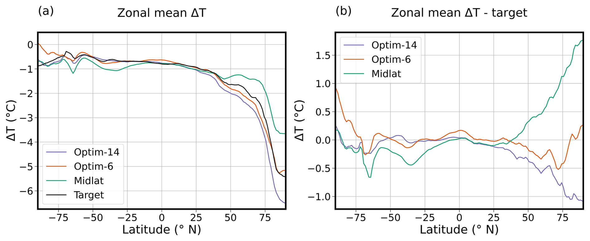
Figure 13 (a) Zonal mean 2040s surface air temperature anomaly (ΔT) for Optim-14, Optim-6, and Midlat, compared to the SSP2-4.5 2014–2033 minus 2040s target. Panel (b) shows the zonal mean ΔT difference between the deployments and the target.

There is some success in Optim-14 and Optim-6 in addressing the midlatitude deployment's undercooling of the NH high latitudes, as shown in Fig. 13. These zonal mean plots show that Optim-14 and Optim-6 provide significantly more cooling of the NH high latitudes compared to the midlatitude strategy, owing to the significant deployment in the NO. Optim-14 overcools in this region with respect to the zonal mean target by 1 °C, while Optim-6 matches the target best of the three deployments.

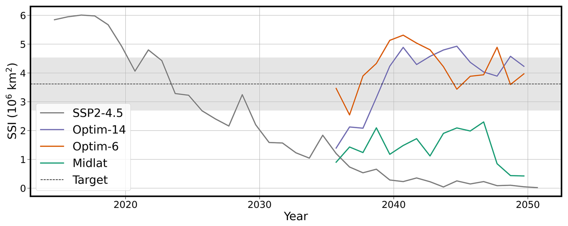
Figure 14 Arctic September sea ice extent (SSI) responses of Optim-14, Optim-6 and Midlat, compared to SSP2-4.5. The dashed line shows the 2014–2033 target and the shading shows the target range used in the methodology to produce Optim-14 and Optim-6, as described in Sect. 4.

Figure 14 shows the SSI response above 60° N. While the Midlat deployment maintains SSI from the start of the deployment in 2035, it fails to restore SSI to the 2014–2033 baseline level. Optim-14 and Optim-6 both restore the sea ice to the target, actually resulting in higher sea ice extent than the 2014–2033 baseline target. Strong Arctic amplification results in significant warming of the Arctic in UKESM1.0, resulting in significant Arctic sea ice loss. MCB deployment design that incorporates sea ice targets, like Optim-14 and Optim-6, prioritise MCB in the NO region to help restore this significant loss in sea ice by focusing more cooling at the NH high latitudes.

Table 4 2040s climate response of Optim-14, Optim-6 and Midlat relative to the SSP2-4.5 control, compared to the target responses. One standard deviation in the annual mean responses is given as a spread of the responses.

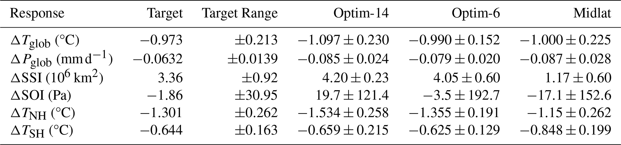
The 2040s mean responses for Optim-14, Optim-6 and Midlat are compared to the targets in Table 4. All three deployments counteract the ΔT_glob rise from the 2014–2033 baseline to the 2040s in SSP2-4.5. Optim-6 achieves the closest match to the ΔT_NH and ΔT_SH targets, and both Optim-14 and Optim-6 manage to restore SSI to above 2014–2033 levels in this model. All three deployments have ΔSOI responses within the target range, with smaller changes to the 2040s mean ΔSOI when compared to the responses to 50 Tg yr⁻¹ MCB deployments in individual regions, as seen in Fig. 6d. The deployments do not have any deployment in the SEP region which has the largest ΔSOI response, although they all include deployment in the SP region which has the second largest ΔSOI response. However, these ΔSOI responses are highly variable as seen in Table 4. Figure S2 in the Supplement shows the SOI timeseries for the three deployments, which shows a small reduction in the standard deviation of SOI that is not statistically significant.

Table 5 As for Table 4, but for Northern Hemispheric mean precipitation anomaly (ΔP_NH), Southern Hemispheric mean precipitation anomaly (ΔP_SH), and ITCZ position.

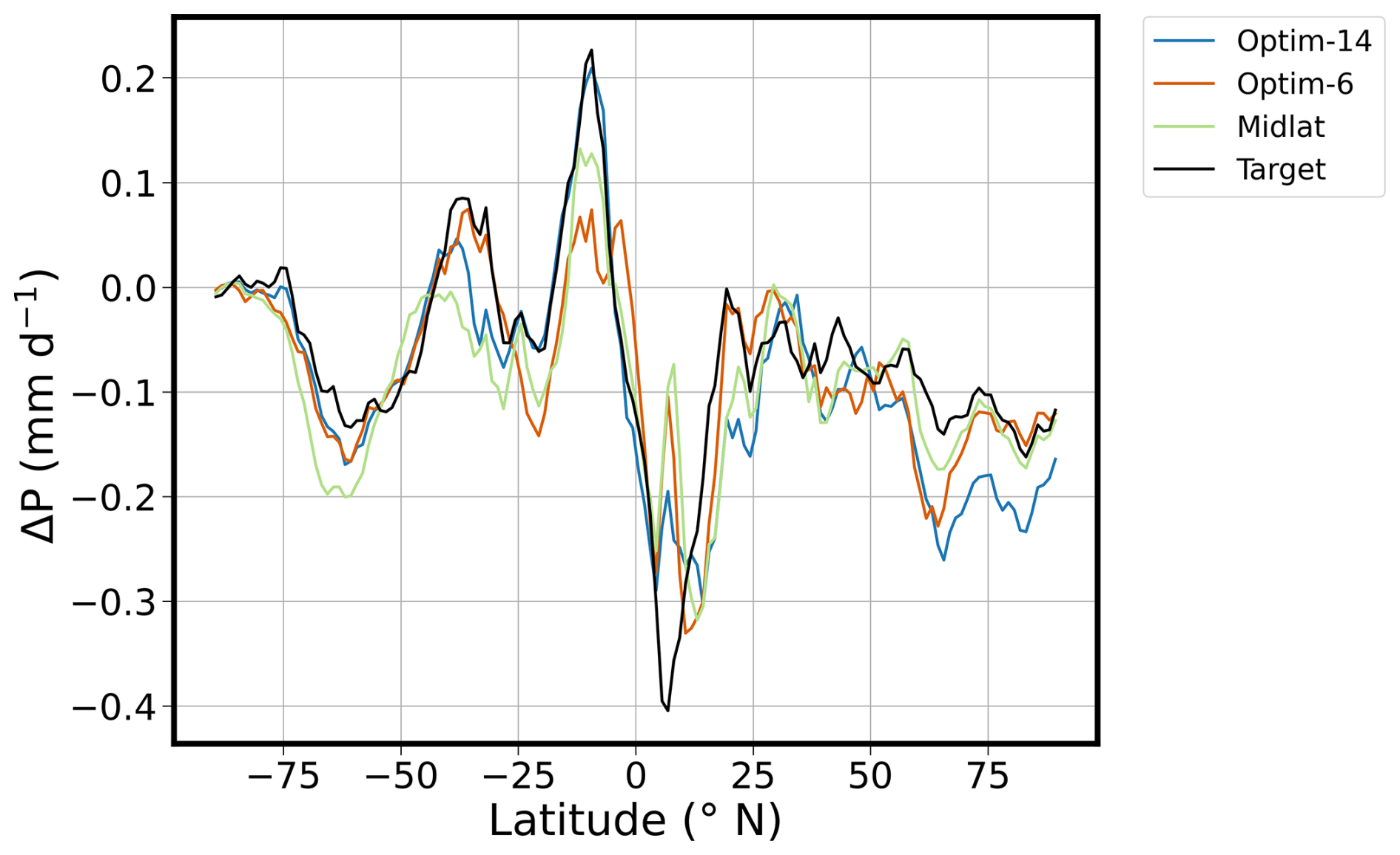
Figure 15 Zonal mean 2040s precipitation anomaly (ΔP) for the Optim-14, Optim-6 and Midlat, with respect to the target restoring the 2014–2033 SSP2-4.5 mean.  

While an ITCZ target was not explicitly incorporated in this optimisation, ensuring balanced ΔT_NH and ΔT_SH responses prevents shifts in tropical precipitation latitude to first order. We verify this in Table 5 which summarises 3 potential targets that could be used following the methodology in this paper; Northern Hemispheric mean precipitation anomaly (ΔP_NH), Southern Hemispheric mean precipitation anomaly (ΔP_SH), and ITCZ position, which is taken to be the latitude position of the precipitation median for precipitation between latitudes 20° N and 20° S (Adam et al., 2016). Optim-14, Optim-6 and Midlat were not optimised for these targets. For ΔP_NH, Optim-6 and Midlat match well with the target and all three simulations counteracting the increase in NH precipitation under SSP2-4.5 for this model. However, all three cause too much SH drying with respect to the ΔP_SH target. Optim-14 has the best match with the target ITCZ position, which agrees with the zonal mean precipitation shown in Fig. 15. Figure 15 shows that all three of Optim-14, Optim-6 and Midlat result in southward shifts of the ITCZ. With respect to the target, all three optimised deployments reproduce similar features, with Optim-14 producing the best match to the target peak at ∼10° S. Optim-14 and Optim-6 both result in too much drying north of 50° N compared to Midlat and the target, which is the result of MCB in the NO region in these two optimised strategies. Incorporating an ITCZ target in future analyses could help further constrain the MCB response on precipitation patterns. However, including larger ensembles and longer runs may be necessary enable a more robust analysis and optimization, particularly on regional precipitation anomalies.

6 Conclusions and Discussion

In this work, we have developed a methodology for optimizing potential MCB deployments, using a base set of simulations to inform optimized deployments that aim to address several climate response targets at once. The methodology was followed to produce two potential deployments, Optim-14 and Optim-6. These deployments were then simulated to test the methodology, with a comparison to a midlatitude deployment, Midlat.

In agreement with the suggestion by Hirasawa et al. (2026a) that a midlatitude deployment may give significant cooling while avoiding the deleterious impacts of strategies targeting subtropical regions, this methodology produces novel MCB strategies that also favour midlatitude regions. Optim-14 and Optim-6 did prioritise some of the midlatitude regions used in Hirasawa et al. (2026a) midlatitude deployment. Significant proportions of the 50 Tg yr⁻¹ were allotted to the NP and SP regions (∼11 % each), and especially the SA region (∼20 %). Differences included the deployment in the WNP region, extending the midlatitude deployment further west. It is important to note this region overlaps with the NP region. This methodology did not incorporate the SI region used in the midlatitude strategy, but resulted in some injection into the SEI region. An analysis incorporating simulations of the SI region, and other MCB patches, in the base set of simulations would be interesting.

The stark difference is the priority of MCB in the NO region, much more apparent in this model owing to the strong Arctic amplification in UKESM1 that results in much greater warming of high latitudes in the NH than CESM2 and E3SM (Henry et al., 2025). The Optim-14 and Optim-6 strategies differ from the Midlat strategy in the emphasis of MCB in the NO (∼30 %), driven by the incorporation of the SSI target. Henry et al. (2025) showed that Arctic sea ice could be maintained across three ESMs with SSA injection between 60 and 80° N, and while the Midlat strategy appears to delay continued reductions in sea ice extent out to the mid to late 2040s, this study suggests that MCB in the NO region may be critical for targeting a restoration of sea ice extent. This analysis indicates that incorporation of MCB in the NO region to compliment a midlatitude strategy is necessary when considering climate response targets like sea ice and hemispheric temperatures.

Using the ever-widening array of MCB data, such as the patch simulations considered in this study, provides an opportunity to search for MCB combinations that have more targets, and there is some strength in optimising MCB to satisfy multiple targets at once, at least for UKESM1. However, the specifics of any “optimised” deployment will depend greatly on the definitions of the targets as well as the models being used. An appreciation of the model dependence of Optim-14 and Optim-6 is vital, and similar analyses using other ESMs for comparison is critical to improve the understanding of uncertainties and risks of any “optimised” MCB strategies. It is likely that the optimal emission distribution will depend on the climate targets. Incorporating spatial correlation into the optimization methodology by emphasising the minimisation of regional scale differences from a target period, rather than just targeting large scale climate metrics, could reduce some of the residual regional warming or precipitation changes that remain in Optim-14 and Optim-6 (Brody et al., 2025).

Moreover, this study relies on a single 15-year coupled simulations for each region and given injection rate, which is a significant limitation of this analysis. Longer simulations and/or larger ensembles would help to improve this analysis by allowing better uncertainty quantification and enabling the development of more robust optimised strategies. Longer simulations would allow for more sophisticated analyses of the impacts of MCB on ENSO. Alternative targets that consider the magnitude and frequency of El Niño and La Niña events, along with ITCZ targets, would be interesting to incorporate into future optimisation analyses. MCB could potentially play a role in reducing strong ENSO events as suggested by Wan et al. (2026), motivating further research into the potential and risks of MCB used to target specific ENSO events to mitigate extremes.