Long-term trends in reconstructed atmospheric aerosol load based on large-scale sunshine duration records since 1900

Aerosol emissions from anthropogenic sources have increased considerably since pre-industrial times. However, global climate models exhibit substantial discrepancies in the radiative forcing attributed to anthropogenic aerosols, a primary factor contributing to uncertainties in total anthropogenic forcing estimates. Therefore, achieving a sufficiently accurate quantification of historical aerosol optical depth (AOD) would be crucial to enhance our ability to project future climate changes and formulate effective mitigation and adaptation strategies. This study uses multiple observational networks, utilizing sunshine duration as a proxy for broadband AOD (BAOD), together with cloud cover observations from 2700 sites across the world, to reconstruct BAOD trends since the late 19th century. In particular, this analysis provides, for the first time, historical BAOD estimates for Europe dating back to the early 1900s. The findings include a general trend toward cleaner atmospheres at most European observation sites during both the 1900–1925 and 1926–1959 periods, amounting to regional trends of −0.014 and −0.004 per decade, respectively. The mean-annual BAOD is found to increase at only a few stations during those periods, likely because of local industrialization. Conversely, based on sunshine data from around 400 sites during the 1960–1985 period, the analysis, underscores the role of anthropogenic aerosols in the dimming observed across Europe (0.004 per decade), as well as the modulating relevance of volcanic aerosols. A continuous increase in BAOD is also observed over Southeast Brazil during 1960–1985, with a noticeable higher rate of 0.015 per decade, which is approximately four times as large as that found in Europe. At the same time, Japan experienced a notable decrease in BAOD with a rate of −0.015 per decade, owing to stringent environmental regulations implemented between 1960 and 1985. Meanwhile, Oceania exhibited a modest negative trend of −0.004 per decade during that period. During the 1986–2015 period, commonly referred to as a “brightening phase”, a general decline of annual BAOD is observed in each studied region: higher rate of decreasing aerosol load in Southeast Brazil, Japan, and Europe by −0.010, −0.015, and −0.013 per decade, respectively, compared to much lower rate of −0.003 per decade over Oceania. This comprehensive assessment sheds new light on the historical BAOD variability and highlights region-specific differences, contributing valuable insights that can help refine climate models and advance our understanding of the complex interplay between aerosols and climate.

1 Introduction

Projections of climate change, a key information for decision-makers, still include large uncertainties caused partially by atmospheric aerosols (IPCC Sixth Assessment Report; Rosenfeld et al., 2014; Stevens, 2013). A significant source of uncertainty originates from our limited knowledge of the historical evolution of aerosol load (Storelvmo et al., 2018; Moseid et al., 2020). To estimate the relative contribution of anthropogenic aerosols to the aerosol forcing, it is important to know how much anthropogenic aerosol emissions perturb the level of background aerosol from natural sources (Carslaw et al., 2013), although it is possible that a part of the observed changes in aerosol load has been caused by changes in natural aerosol emissions from climate feedback. In addition, the separate impacts of aerosols, water vapor, and clouds on the long-term or decadal trends – usually referred to as dimming/brightening – in the observed surface solar radiation (SSR) is not yet well-established (Wild, 2009, 2016; Schilliger et al., 2024). Therefore, the scientific community is still looking for an accurate historical time-series of aerosol load at large scale to enhance the reliability of Earth Systems Models (ESM) when estimating the climate sensitivity to aerosols.

A major source of uncertainty in aerosol–climate interactions is related to the limited availability of long, observation-based records of aerosol optical depth (AOD), especially prior to the satellite era. Ground-based sunphotometer AOD observations (e.g., AErosol RObotic NETwork abbreviated AERONET) provide high-quality reference measurements but began only in the early 1990s (Holben et al., 1998), at which time the network counted only a few stations. In parallel, the earliest satellite-based AOD products extend back only to the late 1970s, with rough AOD estimates obtained with retrievals from the Total Ozone Mapping Spectrometer (Torres et al., 2002).

Longer, observation-based proxies for AOD are valuable for multiple purposes, including characterizing historical variability and providing benchmarks for the quantification of aerosol evolution in global climate models. Because aerosols modulate radiative transfer through the atmosphere, the scarcity of long AOD records also limits our ability to interpret multi-decadal changes in surface solar radiation, including the reported dimming/brightening.

Long-term changes in surface solar radiation (“dimming/brightening”) reflect contributions from aerosols, clouds, water vapor, and circulation-driven variability. Because of their complexity, the relative roles of these factors remain challenging to disentangle from the available observations alone. Nevertheless, long time series of aerosol burden can provide valuable complementary evidence by documenting the timing and spatial coherence of changes in AOD. In particular, the early-twentieth-century brightening signals that were reported over some regions motivate an increase in effort to extend observation-based aerosol burden proxies further back in time, while recognizing that burden changes alone do not uniquely determine causation.

To infer AOD at many locations before the 1970s, the best would be to rely on solar radiation/pyrheliometric observations of direct solar irradiance, from which AOD or other turbidity related parameters can be inferred through an inversion approach (Gueymard, 1998; Russak et al., 2007; Qiu, 2003) with reasonable accuracy (Carlund et al., 2003). Since such old records are extremely rare (Lachat and Wehrli, 2013), the next best solution is to use long-term ground-based sunshine duration (SD) measurements instead. These have become a useful proxy because their records have been available at a few sites as early as the 1880s (Matuszko and Węglarczyk, 2015; Sanchez-Romero et al., 2016; Dumitrescu et al., 2017; Wandji Nyamsi et al., 2020) and have become widespread at the beginning of the 20th century (Urban et al., 2018). Since clear-sky conditions are required for the estimation of AOD from these measurements (Jaenicke and Kasten, 1978; Helmes and Jaenicke, 1984; Eltbaakh et al., 2012; Sanchez-Romero et al., 2014, 2016; Dumitrescu et al., 2017; Wandji Nyamsi et al., 2020), cloud information, such as total cloud cover (TCC), becomes a crucial supplementary meteorological variable to help filter out the effects of clouds on SD in these prominent records.

Several approaches have been developed and applied to estimate AOD at daily scale from SD measurements over Europe with Romania and Spain and Northern China (Sanchez-Romero et al., 2016; Li et al., 2016; Dumitrescu et al., 2017). A recent “hybrid” method by Wandji Nyamsi et al. (2020) enabled an accurate reconstruction of the historical evolution of AOD, fitting within this topic. It is a fully physics-based method combining the best aspects from previous studies by Li et al. (2016), Sanchez-Romero et al. (2016), and Dumitrescu et al. (2017), with further enhancements in some parts. Similar to the sunphotometer-based approach widely used within AERONET, the hybrid method exploits a more accurate broadband direct normal irradiance (DNI) model than the one used in Li et al. (2016)'s approach and takes into account local conditions affecting SD measurements through the seasonal variability of the burning threshold of the Campbell-Stokes heliographs used for SD observation. A description of the hybrid method is detailed in Sect. 3.3.

One critical difficulty that must be resolved to generalize the hybrid method, however, is that combined datasets of historical SD and TCC time series are difficult to find at global scale. For instance, previous studies of this kind were limited to only one or a few stations (e.g., Matuszko, 2012; Vetter and Wechsung, 2015, Wild et al., 2021; Montero-Martín et al., 2021, 2023; Aparicio et al., 2023). The objectives of the present study are thus twofold: (i) uncover as many SD-TCC combined datasets as possible over all continents; and (ii) develop the first historical observation-based AOD database for a long period starting from the early 1900s. The ultimate scientific goal is to provide detailed information on the historical evolution of AOD, desirably including pre-industrial conditions. More specifically, this goal can be broken up into obtaining reliable, multidecadal AOD time series, detecting their long-term trends over different parts of the world, connecting them with anthropogenic aerosol emissions, and separating them from natural sources of variability caused by volcanic activity, dust storms, or wildfires. Although this effort is unprecedented in terms of number of stations investigated in many parts of the world, and in terms of duration of the uncovered time series of the distant past, it is acknowledged that the available datasets only cover a small part of the world. Obviously, the farther through the past an empirical investigation is conducted, the lower number of observing stations is available and the higher the risk is for incomplete or questionable data. Considering this important limitation, it is emphasized that the present regional results of the early 20th century are fragmentary and cannot be truly generalizable to the global scale.

2 Sources of data

For maximum transparency and reproducibility, all measured and modelled data used in this study can be freely accessed through public sources available on the web or are available from the authors upon request. Details on access are specified in this section and are summarized in the “Data Availability” section.

2.1 Sunshine duration and total cloud cover measurements

SD has been observed over many decades by means of dedicated heliographs that record the burned trace of concentrated direct irradiance on a special paper chart. The vast majority of stations have used the Campbell-Stokes type of heliograph, which is used here exclusively, with one exception (see Sect. 3.2). (Other instrument designs have existed and have been used in, e.g., the U.S., but do not provide compatible SD readings.) Additionally, TCC is a crucial parameter used for selecting clear days. It is defined as the fraction of the sky obscured by any type of cloud as observed from a given location, typically expressed in eighths (oktas) or percent. It takes into account all cloud layers combined; a clear sky is $\mathrm{0}/\mathrm{8}$ (or 0 %), whereas a sky completely obscured by clouds is $\mathrm{8}/\mathrm{8}$ (or 100 %).

Extensive efforts have been devoted to uncovering all the available SD and TCC measurements in databases such as the World Radiation Data Centre (http://wrdc.mgo.rssi.ru/, last access: 1 September 2022). Both SD and TCC measurements are also found in the European Climate Assessment & Dataset (ECA&D, https://www.ecad.eu, last access: 1 September 2022). Quality-controlled climate data from German stations, namely temperature, pressure, precipitation, sunshine duration, etc., are collected and distributed by the German Meteorological Service (Deutscher Wetterdienst, DWD) via its Climate Data Center (CDC, https://opendata.dwd.de/climate_environment/CDC/observations_germany/climate/daily/kl/, last access: 1 September 2022). Another worldwide source of data for both daily SD and TCC is the Integrated Surface Database (ISD, https://www.ncei.noaa.gov/access/search/data-search/global-historical-climatology-network-hourly, last access: 1 March 2025; Smith et al., 2011). In addition, several world institutions that are well known for the quality of their meteorological measurements, such as national weather and meteorological services, were contacted directly and individually by email.

After data collection, Europe emerged as the continent offering the largest number of stations providing both SD and TCC, along with the longest temporal coverage. Nevertheless, suitable measurements were also obtained from other parts of the world, e.g., Asia, North Africa, South America, and Oceania. All these regions are investigated here.

To be considered usable, the stations observing SD and TCC had to be collocated at a maximum distance of 50 km. Overall, the compilation yielded about 2700 stations distributed over 20 countries in five continents.

2.2 ECMWF total column amounts of water vapor and ozone

Here, daily-mean estimates of the total column amounts of water vapor, l_w, and ozone, l_o, have been obtained from the European Centre for Medium-range Weather Forecasts (ECMWF) 20th century reanalysis, ERA-20C (https://www.ecmwf.int/en/forecasts/datasets/reanalysis-datasets/era-20c, last access 1 September 2022), which covers the period from January 1900 to December 2010 (Poli et al., 2016). This data source has been specifically selected because it is one of the longest reanalysis products, thus covering most of the reconstruction temporal period investigated in this study. Moreover, it has been widely used in various disciplines, based on its reported accuracy. ERA-20C is produced with a modern data-assimilation system; however, because the density of assimilated surface observations decreases markedly backward in time, the uncertainty in model-derived fields is expected to be larger during the early decades and over sparsely observed regions.

The estimated variables have a spatial resolution of ∼ 1.125° over the whole globe. The daily means of l_w and l_o are extracted from the closest pixel to the location under scrutiny. They are both needed as inputs to the hybrid method described in Sect. 3.3 to remove the atmospheric attenuation caused by water vapor and ozone. The ECMWF l_o data are used from 1 October 2004 backwards.

2.3 OMI total column amount of ozone

Daily l_o data are also provided by the Ozone Monitoring Instrument (OMI) on board the NASA EOS Aura spacecraft since 9 August 2004. Numerous analyses have reported the high quality of these l_o retrievals when compared against relevant ground-based measurements (Balis et al., 2007; McPeters et al., 2008; Antón et al., 2009). The selected data time series are accessible online (https://acdisc.gesdisc.eosdis.nasa.gov/data/Aura_OMI_Level3/OMTO3d.003/, last access: 1 September 2025, https://doi.org/10.5067/Aura/OMI/DATA3001, Bhartia, 2012) since 1 October 2004. The OMI l_o data are used from 1 October 2004 onwards. Overall, it is emphasized that l_o has only a very small impact – if not negligible – on the accuracy of the retrieved AOD (Wandji Nyamsi et al., 2020), therefore the selection and accuracy of its data source are of limited importance.

2.4 MERRA-2 reanalysis aerosol products

Among other products, NASA's Global Modeling and Assimilation Office has produced the Modern-Era Retrospective analysis for Research and Applications, Version 2 (MERRA-2) reanalysis, which includes a multi-parameter aerosol product (Gelaro et al., 2017). This product is selected here to provide the assimilated aerosol information because several studies have demonstrated the quality of its AOD estimates, most importantly (e.g., Gueymard and Yang, 2020).

MERRA-2 assimilates numerous sensors and ground-based measurements. Regarding aerosols in particular, the assimilation includes ground-based measurements from AERONET, two Moderate Resolution Imaging Spectroradiometer (MODIS) sensors flying on board both Terra (morning overpass since 2000) and Aqua (afternoon overpass since 2002) satellites, Multi-angle Imaging SpectroRadiometer (MISR) data from the Terra satellite, and Advanced Very High Resolution Radiometer (AVHRR) data from NOAA Polar Operational Environmental Satellites (Randles et al., 2017). The MERRA-2 products cover the period from 1980 to the present with a spatial resolution of 0.5° latitude × 0.625° longitude (Molod et al., 2015). This study uses the hourly total aerosol extinction AOD at 550 nm and total aerosol Ångström exponent (470–870 nm) available from the MERRA-2 repository (http://disc.sci.gsfc.nasa.gov/mdisc/, last access: 1 June 2020). All hourly data between sunrise and sunset are averaged to retrieve the daily sun-up MERRA-2 estimates.

3 Methodology

The fundamental question of how the historical AOD levels have evolved during past decades is addressed here based on the method detailed in Wandji Nyamsi et al. (2020), which estimates the daily AOD from SD measurements under assumed clear-sky conditions. In order to rigorously carrying out this research, the methodology is split into three steps: (1) perform homogeneity tests to select a reasonable set of ground-based stations with good-quality measurements; (2) apply Wandji Nyamsi et al. (2020)'s method to estimate AOD from SD under clear-sky conditions at each site; and (3) evaluate the decadal trends over each estimated historical evolution of atmospheric aerosol load at each site. An overview of the methodology is given in Appendix B.

3.1 Homogeneity tests

For this study, highly homogeneous time series of SD measurements are needed to ensure the best quality of results. Here, a time series is considered homogeneous if it is impacted only negligibly by non-climatic factors, following careful application of the set of homogenization tests described hereafter. A preliminary step consists of a series of efficient homogeneity tests, jointly referred to as “homogeneity algorithm” (HA). HA is appropriately designed first to detect any obvious artefacts in the time series. The analysis involves both SD and the corresponding SD fraction (SDF), obtained after normalizing the daily SD by that day's sunup hours. Both the SD and SDF time series from each individual station are then scrutinized. The yearly mean (Mean), mean of the monthly maximum per year (Max), and standard deviation of the monthly maximum per year (Std) are calculated from both the SD and SDF time series. This yields a total of six variables to be tested, describing the temporal SD variations and representing important characteristics of variation at yearly scale. A series of four homogeneity tests of the literature is then applied sequentially to each annual time series of the six aforementioned variables: (i) the standard normal homogeneity test (Alexandersson, 1986); (ii) the Buishand range test (Buishand, 1982); (iii) the Pettitt test (Pettitt, 1979); and (iv) the Bartlett's test for homoscedasticity (Bartlett, 1937). The four tests are applied to each variable with a confidence level of 99 %. If at least three of four tests have statistically significant detected inhomogeneities, the median year obtained by the three first homogeneity tests is categorized as a change point for that variable. However, a change point is mostly caused by either one of two types of reasons: (1) non-climatic factors such as change in instrumentation, observing practices, location, or environment; or (2) climatic factors such as natural phenomena (e.g., volcanic eruptions) or change from a dimming to a brightening period, or vice versa (Toreti et al., 2011). Because the change point detection helps to identify an inhomogeneous time series, a discrimination between Type-1 and Type-2 change points is obviously required. A qualitative assessment is performed to resolve this kind of situation. An exhaustive literature describes the typical climatic factors that can cause change points in a time series that is actually homogeneous. Based on that, the timing of massive volcanic eruptions and approximate years of change from dimming to brightening phenomena can reasonably represent the climatic factors associated with change points.

The median year that is categorized as a change point for one analysed variable is retained only if that year is not amongst potential years of previously listed climatic factors. Then, the four homogeneity tests are applied anew on each of the five remaining variables, thus resulting in a total of six analysed variables as mentioned earlier.

Let Y_i denotes the retained median year of the ith analysed variable, $\forall i\mathit{ϵ}\left\{\mathrm{1},\mathrm{2},\mathrm{\dots },\mathrm{6}\right\}$. Y_i is collected and gathered in a set {Y_i}. At this step, two situations exist. First, the set is empty, i.e. no retained years were found; the SD time series is thus considered homogeneous. Second, the set is not empty so that an action is executed as follows. The number of occurrences of Y_i is counted. If Y_i or Y_i+1 had two occurrences at maximum, the SD time series is considered homogeneous too. For at least three occurrences in total, the SD time series is considered inhomogeneous. In that case, the SD time series is split into two sub-SD time series from the most recent year (reaching up to three occurrences) (1) backwards and (2) onwards. Only onwards sub-SD time series as the reduced time series, is retained because, following the development of ground- and satellite-based instruments, recent data are generally more homogeneous than old data.

Afterwards, HA is iteratively applied as described previously until no change point is further detected within a reduced time series. When the analysed time series is change-point-free related to non-climatic factors, the time series is finally retained for further analysis. The TCC time series are analysed in the same way as just described for SD. Only SD and TCC times simultaneously and successfully passing this homogeneity test are retained for further analysis.

3.2 Illustration of the application of the homogeneity algorithm

To demonstrate the efficiency of the HA for SD time series, an example of the results of the four tests is carried out on one of the longest and best maintained operational radiation monitoring stations, namely Potsdam, Germany. Generally associated with each relevant historical SD time series, metadata information is normally the most powerful and reliable way to find out inhomogeneities of station series over the entire period under scrutiny. Over the station's history of the measuring devices for SD at Potsdam, only one important change in observational routines is reported and summarized as follows: SD records are performed (1) from 1 January 1893 to 15 March 2005 with Campbell-Stokes SD recorder and (2) from 16 March 2005 to 11 November 2021 with automatic SD recorder named “SONIe Solar Energy sensor”. There was an overlapping measurement period of both SD sensors between 12 August 1992, and 15 March 2005 to (1) prevent the potential effects during the transition from manual to automatic instrument and (2) for ensuring inhomogeneities-free SD time series. As consequence, SD time series has been proved to be completely homogeneous since 1893 until the present day (Hannak et al., 2019).

Figure 1 shows the results of the standard normal homogeneity test (SNHT), Buishand range, and Pettitt-Bartlett's tests applied to various time series: the yearly mean (Mean_SD, Mean_SDF), mean of the monthly maximum per year (Max_SD, Max_SDF), and standard deviation of the monthly maximum per year (Std_SD, Std_SDF) conveniently computed from the SD and SDF time series of Potsdam. Corresponding test results for Mean_SD, Max_SD, Std_SD, Mean_SDF, Max_SDF, Std_SDF time series are plotted in green, gold, blue, brown, violet and pink respectively for the SNHT, Buishand range, and Pettitt tests. For Bartlett's test, the statistically significant zone, i.e., wherever the p-value is lower than 0.01, is delimited by the light-yellow area. The year of detected change point of each test statistic is reported on the graph close to the variable name.

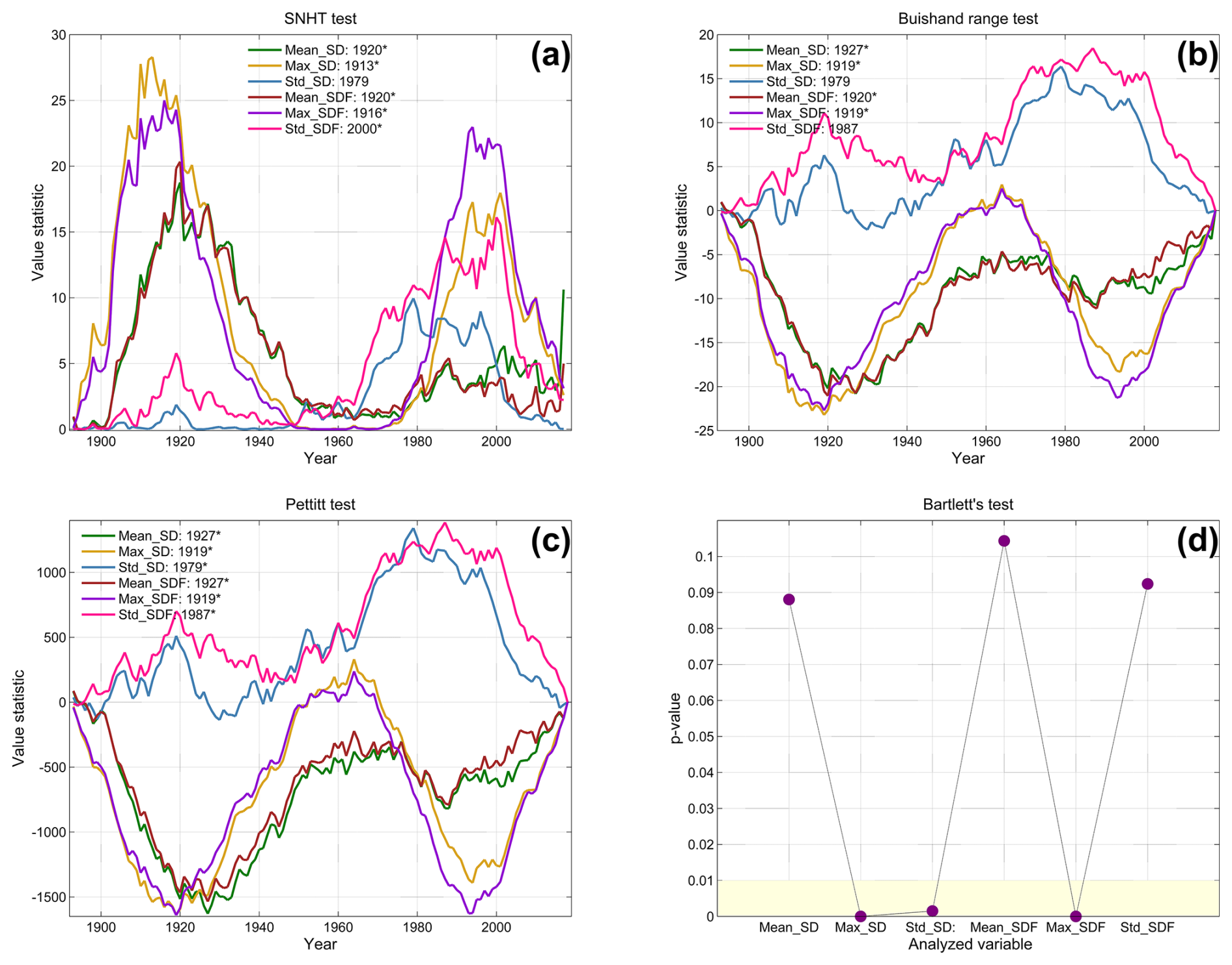
Figure 1 Test results of the (a) SNHT; Buishand range (b), Pettitt (c), and Bartlett's test (d) applied to the time series of six variables at Potsdam, Germany. The year of extreme is indicated. The asterisk indicates that the change point is statistically significant (p<0.01) for the shown year for the analysed variable and used test. A statistically significant (p<0.01) zone is delimited by the light-yellow area for Bartlett's test.

For the Mean_SD time series, the SNHT statistic (Fig. 1a) reaches an extreme in 1920, indicative of a change point around that year. This maximum, or change point, which is statistically significant in 1920 with a p-value lower than 0.01, causes a rejection of the null hypothesis at the 1 % level. Similar conclusions are drawn from the minima in the graphs of the Buishand range and Pettitt test statistics, both having statistically significant extremes in 1927. Conversely, the Bartlett's test does not indicate any inhomogeneity at the 1 % level. Nevertheless, since three tests reject the null hypothesis at the 1 % level, the median year 1927 is kept for further analysis and categorized as a change point for Mean_SD time series.

The same procedure is repeated and applied on each of the five other variables of interest, as investigated just above. As result, the change point is statistically significant in 1919, 1920, and 1919 for the Max_SD, Mean_SDF, and Max_SDF time series, respectively. In summary, the occurrences of statistically significant change points are 2, 1, and 1 for 1919, 1920, and 1927, respectively. There is no year having at least three occurrences in total. Therefore, the SD series of Potsdam is assigned to be a homogeneous time series over the entire time period, which is perfectly corroborated by the metadata information. Hence, that time series can indeed be used for trend computations.

More generally, the HA method has been tested on a reduced set of 58 SD time series from stations having available metadata information serving as reference for the identification of non-climatic change points. About 96 % of the time, HA was found to accurately categorize homogeneous time series by clearly detecting the potential change points associated with non-climatic factors.

3.3 Estimating daily AOD from SD measurements

The daily-mean AOD is estimated from SD data using the hybrid method developed by Wandji Nyamsi et al. (2020). The concept of this method is elaborated in a step-by-step approach as follows. In the context of historical observations, SD is the total length of the burned trace on an appropriate card of the Campbell-Stokes heliograph. Each card represents data over one specific day. The burned trace appears when DNI is greater than the burning threshold of the card. During a cloudless day, – the sky condition of interest in this paper – the burned trace is expected to be continuous; it starts not long after sunrise and stops just before sunset. Assuming the diurnal uniformity of daily ozone and water vapor conditions, the SD-derived AOD can also be considered diurnally uniform. Consequently, SD can be transformed to an equivalent hour angle (ω) such as $\mathit{\omega }=\mathrm{15}(\frac{\mathrm{SD}}{\mathrm{2}}$) in degrees. From an hour angle, in turn, with the latitude of the station and solar declination angle at a given day, both accurately known, the solar zenith angle (θ_s) can be computed. Then, θ_s is used to compute air masses and all atmospheric transmittances using the mathematical equations explicitly given in Appendix A. These equations are used to finally derive AOD as described hereafter. With this approach based on the computed θ_s, the SD-derived AOD is estimated at those instants close to sunrise/sunset, when the burned trace becomes visible/extinct, respectively.

Concretely, for each ground-based station retained after applying the preliminary HA, a selection of SD data under cloudless days is carried out. A day is assumed to be cloudless if the average of daily available TCC observations is rounded to 0 okta. Depending on the type of the daily mean of cloud cover available at few stations, without being too restrictive but still realistically close enough of various cloudless days, an exception has been made so that the average of daily available TCC observations is ≤1 okta. This threshold is typically used in the literature, rather than 0 okta, as a valid trade-off between accurate selection and reasonable number of cloud-free days having no significant influence on the computed AOD trends (Manara et al., 2016; Yang et al., 2019; Wild et al., 2021). Cloudless SD data combined with atmospheric variables such as l_w, l_o, and the MERRA-2 aerosol products are conveniently used to estimate the monthly burning threshold of each Campbell-Stokes instrument from year 2000 onwards. This is done by using a reliable broadband DNI model proposed by Wandji Nyamsi et al. (2020) based on accurate functions for broadband transmittance and optical mass of each attenuator identified in Gueymard (2003). These functions are then tested with an improved version of the absorption parametrization named kato2andwandji that is included in libRadtran (Kato et al., 1999; Mayer and Kylling, 2005; Wandji Nyamsi et al., 2014, 2015a; Emde et al., 2016). A theoretical validation of these functions was conducted under an appropriate set of realistic atmospheric conditions as used by e.g., Wandji Nyamsi et al. (2015b, 2017, 2019, 2021, 2026). Detailed information on this method appears in Wandji Nyamsi et al. (2020). All the equations needed to derive the broadband DNI used here are explicitly given in the Appendix.

A monthly climatology of daily l_w and l_o over the period 1900–1925 is computed from daily l_w and l_o data extracted from the ERA-20C reanalysis over the period 1900–2010 (Poli et al., 2016). To some extent, the computed climatology is assumed for daily atmospheric inputs before the year 1900. A computed daily l_w and l_o from the Copernicus Atmosphere Monitoring Service (CAMS) is used from 2011 onwards. The atmospheric aerosol load is characterised here in terms of the daily broadband AOD, BAOD or τ_a, according to its original definition (Unsworth and Monteith, 1972):

$$\begin{array}{}\text{(1)}& {\mathit{\tau }}_{\mathrm{a}}=-\ln \left(T_{\mathrm{a}}\right)/m_{\mathrm{a}}\end{array}$$

where T_a is the atmospheric transmittance for the total aerosol attenuation over the shortwave and m_a is the aerosol optical mass. In practice, T_a is unknown and must be estimated indirectly. Based on the data available in the present context, T_a is evaluated from:

$$\begin{array}{}\text{(2)}& T_{\mathrm{a}}={\displaystyle \frac{\stackrel{\mathrm{‾}}{G_{\mathrm{b}}}\left(mm\right)}{\mathit{\epsilon }{G}_{\mathrm{o}}{T}_{\mathrm{R}}{T}_{\mathrm{g}}{T}_{\mathrm{o}}{T}_{\mathrm{w}}}}\end{array}$$

where mm is the month number, $\stackrel{\mathrm{‾}}{G_{\mathrm{b}}}\left(mm\right)$ is the computed monthly-effective burning threshold irradiance of the Campbell-Stokes heliograph under scrutiny, ε is the Sun–Earth distance correction factor (depending on the day of the year), and G_o is the extra-terrestrial irradiance received on a plane normal to the Sun rays, also known as “solar constant”, assumed here to be 1367 W m⁻² as originally used by, e.g., Li et al. (2016) or Wandji Nyamsi et al. (2020) and adopted based on the recommendation of the World Meteorological Organization. Finally, T_R, T_g, T_o, and T_w are the individual broadband transmittances of the main non-aerosol attenuators, i.e., Rayleigh scattering, uniformly mixed gases, ozone absorption, and water vapor absorption, respectively.

From the literature, BAOD is often assumed approximately equal to the spectral AOD at an effective wavelength of 750 nm (Qiu, 1998; Molineaux et al., 1998; Li et al., 2016; Kudo et al., 2012). In reality, this effective wavelength depends on atmospheric variables describing the actual atmospheric state such as air mass, Ångström exponent, and total column amounts of water vapor (Qiu, 2001, 2003). Nevertheless, a few preliminary tests revealed that using a fixed effective wavelength of 750 nm was a reasonable compromise, considering that the true atmospheric state is not always known precisely, especially during the reconstruction period.

The complete Wandji Nyamsi et al. (2020)'s method was originally validated by comparing its BAOD estimates to collocated AERONET measurements serving as reference. This validation was performed at 10 ground-based stations located in Europe under various climates. In general, the correlation coefficient was found greater than 0.6. The bias between estimates and reference values was close to 0.00, with a root mean square difference of 0.07 for the whole sample. These results reveal a reasonable level of accuracy for the method. Furthermore, the uncertainty in the BAOD estimates has been quantified by means of a diagnostic method (Sayer et al., 2020) that uses the expected error (EE_AOD) envelope of BAOD estimates relative to AERONET measurements. This approach includes all possible sources of uncertainties caused by, e.g., changes of burning card type, burning threshold, cloud contamination, changes in aerosol properties during the day, observer errors in sunshine duration or cloud information estimates, input data inadequacies, and the method itself. Overall, the expected error envelope is obtained as ${\mathrm{EE}}_{\mathrm{BAOD}}=\pm (\mathrm{0.01}+\mathrm{0.40}\times \mathrm{BAOD})$. For more detailed information on this method, validation results and performance statistics altogether already developed, carried out and presented, the reader is referred to Wandji Nyamsi and al. (2020).

It is obviously desirable to reduce the impact on the BAOD estimates caused by the uncertainties and systematic biases described above, while also making it possible to correctly interpret any change in the past aerosol loads. To address the key science question of how the historical AOD levels have evolved during many past decades, the daily BAOD estimates elaborated above are converted into seasonal and annual means and are then carefully examined. The seasonal mean is computed as the average of all available daily values over a given season. The four seasons are grouped as follows: December–January–February (DJF), March–April–May (MAM), June–July–August (JJA), and September–October–November (SON). Similarly, the annual mean is computed as the average of all available daily values from 1 December to 30 November of the following year.

To further minimise the uncertainties or biases, anomaly values (relative to the corresponding long-term average) are also analysed, assuming that trends can be more accurately modelled and analysed based on anomaly values rather than absolute values. Therefore, long-term seasonal/annual means are computed as the average of all available seasonal/annual values from 1980 onwards. Then, anomaly values are simply obtained as the difference between a value for a given year and its corresponding long-term mean.

3.4 Trend computations

To detect long-term trends, the subdivision of the entire temporal period covering all available SD measurements is crucial, but still profoundly challenging, because well-known phenomena (e.g., dimming/brightening) or their reversal might not necessarily occur at the same time at all locations. In addition, aerosol events from volcanic activity, dust storms, or wildfires might not locally affect the atmosphere with the same magnitude everywhere. This makes, for instance, the atmosphere much hazier at sites close to a volcano hotbed than at a remote location.

Based on the challenges just described, the whole 1900–2015 period has been intentionally divided into four sub-periods, namely 1900–1925, 1926–1959, 1960–1985, and 1986–2015. This subdivision is made in two steps. The first one makes use of the well-documented dimming and brightening periods that approximately occurred over 1960–1985 and 1986–2015, respectively even though these phenomena are fundamentally local. Nevertheless, it is also assumed that these phenomena, which were originally observed at a few sites, would be representative of the situation at larger scale. The second step concerns the period 1900–1959. The inflection period, 1925–1926, was found after scrutinizing the years of apparent reversal trend from a few long BAOD time series in Europe, in parallel with the corresponding SSR time series, if available, as well as previous findings from the substantial literature on this topic (Ohmura and Lang, 1989; Stanhill and Moreshet, 1992; Stanhill and Cohen, 2001; Ohmura, 2006; Wild, 2009; Wild et al., 2021; Kudo et al., 2012; Antón et al., 2014; Sanchez-Lorenzo et al., 2015; Kazadzis et al., 2018; Moseid et al., 2020; Schilliger et al., 2024). It is acknowledged that other subdivisions of the whole temporal period could have been possible, using different criteria or a different set of stations.

The trend estimates are calculated using the Dynamic Linear Model (DLM) with Markov chain Monte Carlo (MCMC) estimation (Petris et al., 2009, Laine, 2020). The MCMC chain used here has a length of 500, which refers to the number of iterations in the estimation process. Because BAOD time series tend to be log-normally distributed, just as AOD, BAOD is estimated using logarithmic time series. The single model includes a local linear trend component, a seasonal component with regression analysis on a monthly basis, and a first-order autoregressive error term, as described below:

$$\begin{array}{}\text{(3)}& {\displaystyle }{y}_t={\mathit{\mu }}_t+{\mathit{\gamma }}_t+{\mathit{\eta }}_t+{\mathit{\epsilon }}_{\mathrm{obs}},{\mathit{\epsilon }}_{\mathrm{obs}}\sim N\left(\mathrm{0},{\mathit{\sigma }}_t^{\mathrm{2}}\right)\text{(4)}& {\displaystyle }{\mathit{\mu }}_t={\mathit{\mu }}_{t-\mathrm{1}}+{\mathit{\alpha }}_t+{\mathit{\epsilon }}_{\mathrm{level}},{\mathit{\epsilon }}_{\mathrm{level}}\sim N\left(\mathrm{0},{\mathit{\sigma }}_{\mathrm{level}}^{\mathrm{2}}\right)\text{(5)}& {\displaystyle }{\mathit{\alpha }}_t={\mathit{\alpha }}_{t-\mathrm{1}}+{\mathit{\epsilon }}_{\mathrm{trend}},{\mathit{\epsilon }}_{\mathrm{trend}}\sim N\left(\mathrm{0},{\mathit{\sigma }}_{\mathrm{trend}}^{\mathrm{2}}\right)\text{(6)}& {\displaystyle }{\mathit{\eta }}_t=\mathit{\rho }{\mathit{\eta }}_{t-\mathrm{1}}+{\mathit{\epsilon }}_{\mathrm{AR}},{\mathit{\epsilon }}_{\mathrm{AR}}\sim N\left(\mathrm{0},{\mathit{\sigma }}_{\mathrm{AR}}^{\mathrm{2}}\right)\end{array}$$

where y_t is the estimated BAOD at time t; μ_t is the mean level and α_t is the change in the level from time point t−1 to time point t; γ_t is the seasonal component, described by two harmonic components that are each described by trigonometric (sine, cosine) functions; η_t is an autoregressive error component; and ρ is the coefficient for autoregressive component. The Gaussian ε terms are used to evaluate the uncertainties in BAOD estimates (including uncertainty in SD measurements) and in other estimated parameters.

DLM is fitted for the whole BAOD time series. For a given sub-period, the estimated change in BAOD and its uncertainty are defined simultaneously by first sampling the estimated DLM model trend 100 times and then calculating the estimated median and standard deviation of the change for each sub-period of those trend realizations.

Regional trends are finally calculated using bootstrap (Efron, 1981). The bootstrap sample is taken from the estimated trends of stations in the region for the period during which the trend is estimated. The number of stations differs in each period for a variety of reasons. The number of bootstrap samples for each region and time period is 1000, which is assumed to be a large-enough sample for trend uncertainty estimation, i.e., for calculating confidence intervals.

4 Results and discussion

This section provides important results for regions and periods for which no directly observed AOD data have been publicly available. Additional results are included in the Supplementary material. Moreover, computed site-specific trends since 1900 are freely available at the Finnish Meteorological Institute's data repository from https://doi.org/10.57707/fmi-b2share.ae9691880b334499b112fe9d174187ab (Wandji Nyamsi et al., 2025). The data products, i.e. historical evolution of aerosol optical depth, obtained from this study are also available there (https://doi.org/10.57707/fmi-b2share.14e58e89d157468ba155836a72878692, Wandji Nyamsi and Arola, 2025).

4.1 First Period: 1900–1925

At the onset of the 20th century, only six European stations from three countries were found to have SD measurements respecting this study's requirements. Four stations are in Switzerland (Basel, La Chaux-de-Fonds, Neuchatel, and Zurich), one in Germany (Potsdam), and one in Croatia (Zagreb-Gric). Figure 2 shows the spatially distributed decadal BAOD trends computed with a DLM based on annual means for the 1900–1925 period. Over this whole first period, all trends are statistically significant, except at La Chaux-de-Fonds. All computed BAOD trends per season, as well as the corresponding maps, are provided in the Supplement.

The calculated annual BAOD trends range between −0.031 and 0.005 per decade. Four stations, namely Basel, La Chaux-de-Fonds, Neuchatel, and Potsdam, exhibit negative trends of (−0.028 ± 0.004) per decade, (−0.006 ± 0.003) per decade, (−0.031 ± 0.003) per decade, and (−0.022 ± 0.004) per decade, respectively. This denotes a relatively smooth decrease in BAOD. Conversely, for the two remaining stations, positive trends of (+0.003 ± 0.002) per decade and (+0.005 ± 0.001) per decade are seen in Zurich and Zagreb-Gric, respectively.

Five of the world's longest and best maintained operational measurement sites in the world, – among them, Potsdam in Germany, Zurich in Switzerland and Zagreb-Gric in Croatia, previously mentioned, – were selected. These iconic stations have been widely used in the literature on dimming/brightening (Antón et al., 2014, 2017; Wild, 2016; Wild et al., 2021; Sanchez-Lorenzo and Wild, 2012; Sanchez-Romero et al., 2016). Their respective annual BAOD mean time series since the 1900s are plotted in Fig. 3 to help the discussion. The corresponding 5-year running means are displayed too. The 1900–1925 period under investigation here is delimited by the leftmost yellow area in Fig. 3. The few peak values of mean-annual BAOD that are observed over the whole time series reach ≈ 0.3 in 1903 and ≈ 0.25 in 1912 for Potsdam, ≈ 0.15 in 1903 for Zurich, and ≈ 0.1 in 1913 for Zagreb-Gric. These maximum values of BAOD seem to occur around the years of the two world's strongest volcanic eruptions such as Santa María in 1902 and Novarupta in 1912, as indicated by vertical dashed lines in Fig. 3. Impacts on BAOD of massive volcanic eruptions might not be perceptible at yearly scale but can be seen at least at daily scale. This is, for instance, the case for Zagreb-Gric, where the impact of Santa María is not detectable in the annual BAOD mean time series in Fig. 3. At daily scale, however, an elevated peak value of 0.3 has been observed on 27 March 1903, for example. The decreasing trend mentioned earlier for Potsdam is also clearly perceptible in that figure.

The BAOD time series shown in Fig. 3 include both natural background and anthropogenic aerosols. It is difficult to accurately separate those two types of aerosols because of the lack of accurate natural background AOD data, especially during the period under scrutiny. More specialized investigations, out of the scope of this study but still relevant, could be carried out in a future work. Nevertheless, it can be hypothesized that the decreasing trend in Potsdam could be partially the result of the gradual decline of the impact from these massive volcanic aerosol events. For Zagreb-Gric, even if the Novarupta impact is ignored, the increase in AOD can still be observed there and might be partially induced by a surge in aerosol emissions caused by the rapid city development up to the 1914 outbreak of World War I. In most cases, both seasonal and annual trends are consistent in direction with the annual trends shown in Fig. 2.

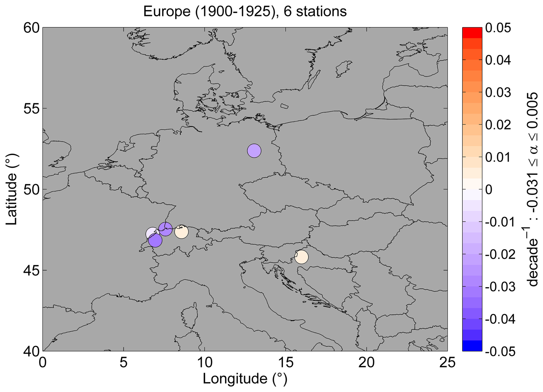
Figure 2 Spatial distribution of decadal BAOD trends based on annual means at six European sites over the period 1900–1925. The number of sites is shown at the top. The colour–coded bar indicates the magnitude of the BAOD trend, whose range is indicated on the side. α represents the trend value computed with DLM.

Using bootstrap, national and regional trends in BAOD are also estimated from the BAOD trends of all the sites that are assumed to be reasonably representative (Efron, 1981). All computed BAOD trends, as well as their standard deviation and a statistical significance index, are provided at the Finnish Meteorological Institute's data repository https://doi.org/10.57707/fmi-b2share.ae9691880b334499b112fe9d174187ab (Wandji Nyamsi et al., 2025) for each site and for each sub-period. In general, negative BAOD trends, (−0.017 ± 0.010) per decade, are obtained over Switzerland during the first period.

For such a period with a very limited number of stations, quantifying a regional trend is highly challenging, mainly because of the spatial scarcity of stations. It is thus to ascertain the effective representativeness of the trend value over that region. This limitation is duly acknowledged, as also mentioned in Sect. 1. Nevertheless, a tentative regional trend value is provided here, as well as for other similar cases. The regional trends calculated from the six baseline stations reach the negative value of (−0.014 ± 0.01) per decade respectively denoting an overall decrease in aerosol load after the major contributions of Santa Maria and Novarupta (Fig. 3).

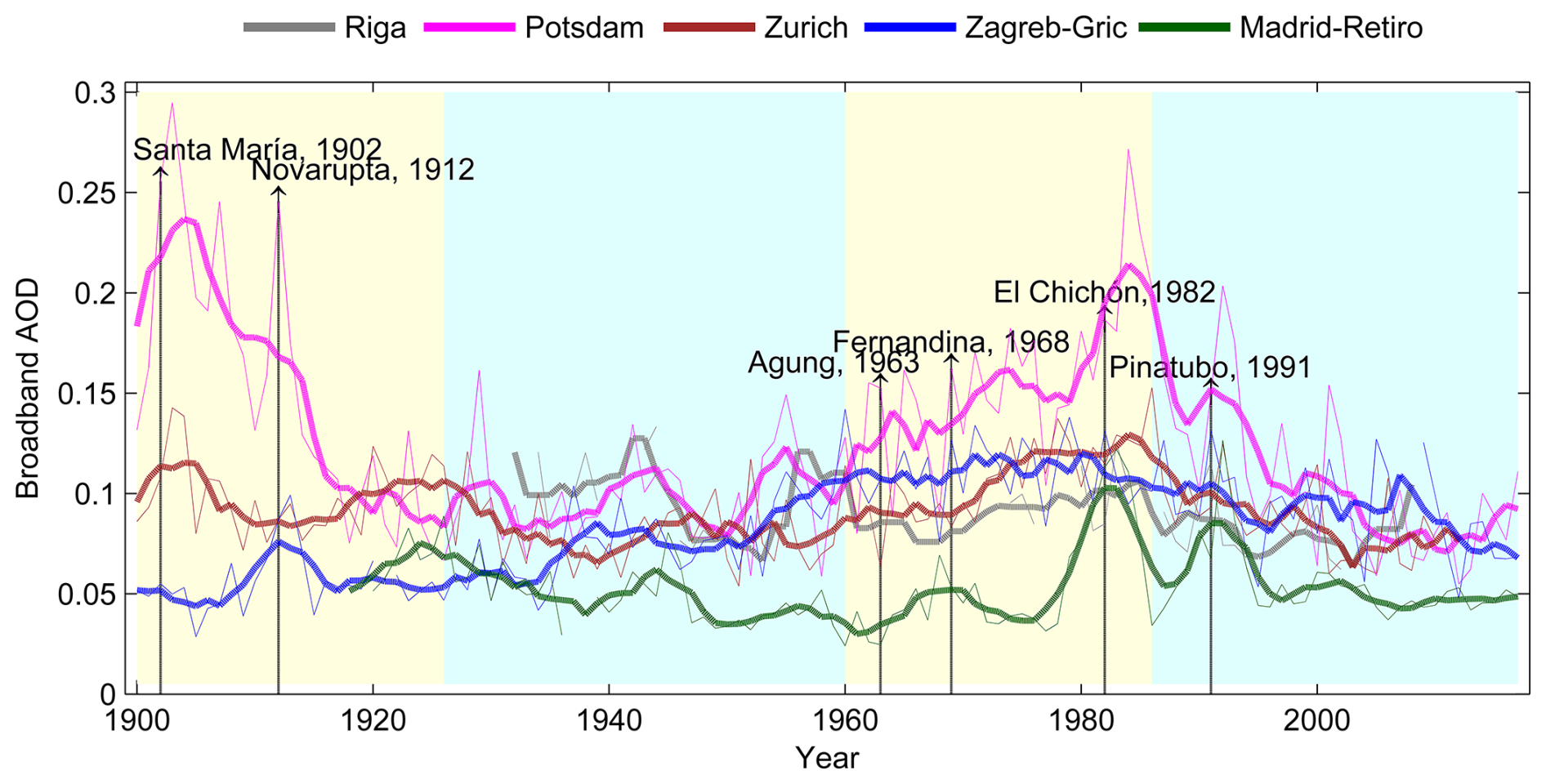
Figure 3 Annual BAOD mean time series since the 1900s for the five longest European measurement sites (coloured thin dashed lines) in decreasing order of latitude: Riga, Latvia (dark grey line), Potsdam, Germany (magenta line), Zurich, Switzerland (brown line), Zagreb-Gric, Croatia (blue line), and Madrid–Retiro, Spain (green line). Vertical dashed lines indicate the years of massive volcanic eruptions. In addition, 5-year running means are shown for all-time series (coloured thick lines).

4.2 Second period: 1926–1959

The BAOD trend map for 1926–1959 is shown in Fig. 4. During this second period, data from only Europe could be found, as before. Compared to the previous period, two more countries are represented, namely Latvia (with the Riga station) and Spain (with the Madrid-Retiro station), as well as three new stations in Germany (Jena-Sternwarte, Geisenheim, Lorch-am-Rhein) and two in Switzerland (Geneva and Sion), for a total of 13 stations. Overall, the trends vary between (−0.013 ± 0.004) per decade (in Riga, Latvia) and (+0.015 ± 0.001) per decade (in Neuchatel, Switzerland). Three stations namely Basel, Potsdam, and Geneva, exhibit nonsignificant trends. Stations that are in the same region generally show consistent trend directions, except for the two closest stations: Neuchâtel and La Chaux-de-Fonds. The disparity between these sites also existed during the first period; it might be caused by the atmospheric stratification (lake boundary layer, inversion layer, and free troposphere) and the main atmospheric flows affecting this tiny area of Switzerland, considering that the sites are located at different elevations: 485 m (Neuchâtel) vs. 1018 m (La Chaux-de-Fonds).

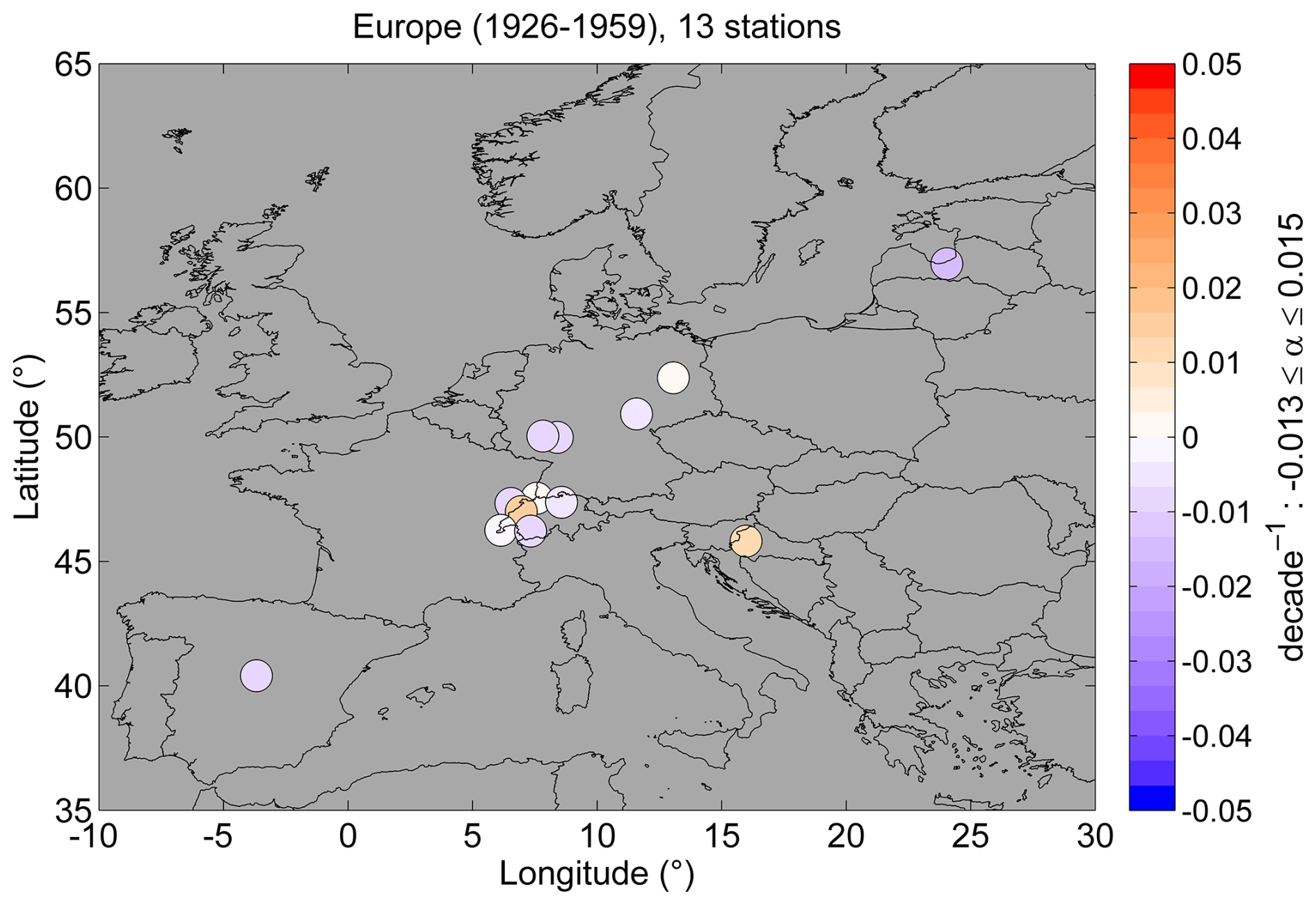
Figure 4 Spatial distribution of decadal BAOD trends based on annual means at 13 sites in Europe during the period 1926–1959. The colour–coded bar indicates the BAOD trend, whose range is indicated on the side. α represents the trend value computed with DLM.

National negative trends of small magnitude are found in Latvia, Germany, Switzerland, and Spain: (−0.013 ± 0.004), (−0.006 ± 0.003), (−0.002 ± 0.004), and (−0.01 ± 0.002) per decade, respectively. Conversely, the trend is positive in Croatia, like during the previous period, and is statistically significant at (+0.013 ± 0.001) per decade. Overall, the European trend is only (−0.004 ± 0.003) per decade, suggesting a slight decrease in AOD at continental scale, hence with no clear or systematic change in aerosol conditions over that period, during which volcanic activity was apparently non-existent. Considering that 61 % of the observational sites have negative TCC trends, both aerosol and cloud changes could have partly contributed to the observed increases in SSR before 1950. This SSR trend, over Europe in particular, has been reported earlier based on measurements from a few radiometric stations only, and is often referred to as the “early brightening” period (Ohmura, 2006; Wild, 2009; Sanchez-Lorenzo et al., 2015).

Compared to the earlier 1900–1925 period, the signs in the national trends are the same, as confirmed in Figs. 2 and 4. The strongest increasing signal at national level, twice that of the trend during the previous period, occurs at Zagreb-Gric in Croatia. This fast-increasing aerosol burden is attributed to a substantial increase in air pollution, likely related to the largest demographic boom in the history of Zagreb, when its population increased by 70 % between 1921 and 1931 (The city of Zagreb, 2007).

4.3 Third period: 1960–1985

Figure 5 shows trend maps over Southeast Brazil, Japan, Oceania (Australia and New Zealand), and Europe. Over Southeast Brazil (Fig. 5a), all trends are found statistically significant. Strong positive trends (greater than +0.015 per decade) are found at São Paulo and São Simão, amounting to (+0.016 ± 0.007) per decade and (+0.018 ± 0.004) per decade, respectively. Conversely, Presidente Prudente was affected by a negative trend, (−0.019 ± 0.008) per decade. This spatial disparity of trends in Brazil could be explained by the rapid industrialisation, which was however concentrated in a small number of locations where an increase in air pollution has been noted (Baer and Mueller, 1995). This increasing BAOD trend, particularly at São Paulo, is an important finding because it confirms the contribution of aerosols to the observed decrease in SSR there, as suggested by Yamasoe et al. (2021).

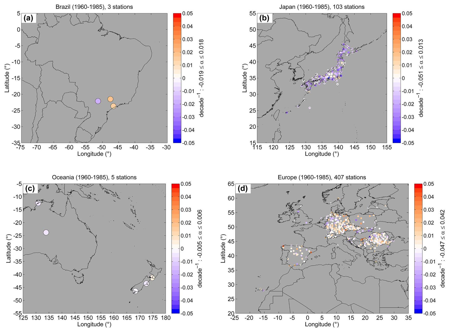
Figure 5 Spatial distribution of decadal BAOD trends based on annual means over (a) Southeast Brazil, (b) Japan, (c) Oceania, and (d) Europe for the period 1960–1985. The number of sites in each region is shown at the top. The colour–coded bar indicates the BAOD trend, whose range is shown on the side. α represents the trend value computed with DLM.

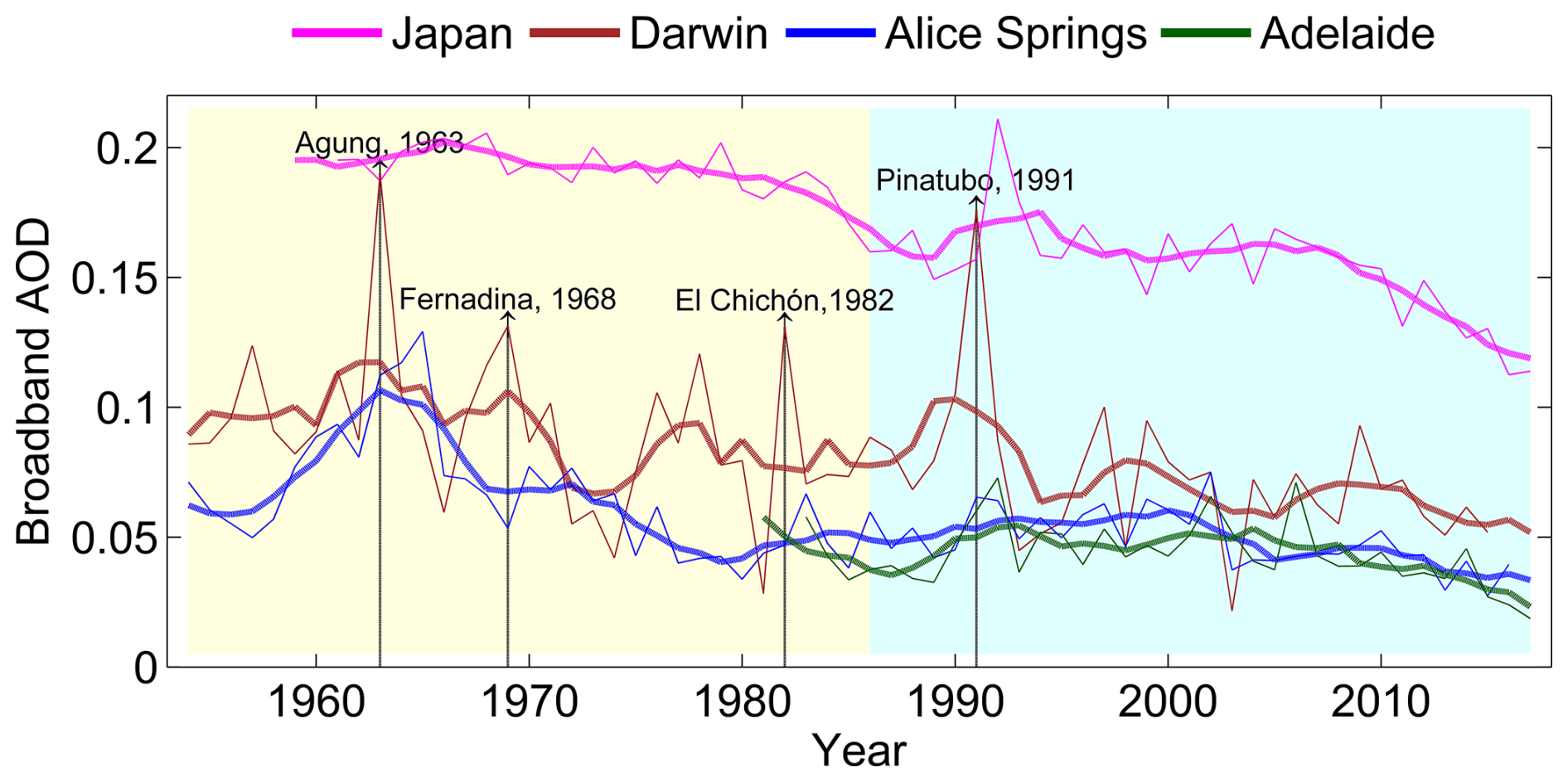
Figure 6 Annual BAOD mean time series over Japan (magenta) from 1960 onwards and over three Australian sites between 1954 and 2016, ordered by decreasing latitude: Darwin (brown line), Alice Springs (blue line), and Adelaide (green line).

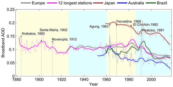
Over Japan, the BAOD trend estimates and the corresponding averaged time series are shown in Figs. 5b and 6, respectively. Remarkably, 71 % of the Japanese sites exhibit statistically significant trends. When only these significant sites are displayed, the corresponding plot of spatial distribution of decadal BAOD trend in Fig. 6 does not differ much from Fig. 5b. This predominantly downward trend over Japan is opposite to the widely reported European dimming: this trend – observed at 89 % of the observational sites, and even at 93 % of them when only statistically significant trends are selected – is most likely caused by a decrease in aerosol emissions. The Japanese national trend found here is statistically significant (−0.015 ± 0.002) per decade and is in very good agreement with earlier findings (Kudo et al., 2012). The proposed explanation is that Japan experienced a serious air pollution problem after World War II because of its strong economic and industrial growth. That in turn led to the adoption of strict air quality policies that were enacted in the 1960s. This resulted in an overall cleaner atmosphere over Japan (Kudo et al., 2012; Ma et al., 2022).

Figure 5c shows the trends over Oceania, based on data from five stations (Darwin and Alice Springs in Australia, and Christchurch Airport, Wellington-Kelburn, and Invercargill Airport in New Zealand). The trends are statistically significant for Christchurch Airport and Wellington-Kelburn. The trends range from (−0.005 ± 0.003) per decade (in Alice Springs) to (+0.006 ± 0.001) per decade (in Wellington-Kelburn). The difference in trends between observational sites is relatively small, resulting in a regional trend that is close to zero.

Despite the limited number of stations over Oceania, it is likely that this region did not experience much aerosol-induced decadal variations in SSR during that period – -at least related to anthropogenic sources. From Fig. 6, however, the BAOD time series at Alice Springs appears more variable than at Darwin, which justifies closer scrutiny. Figure 6 reveals an increasing aerosol load at Alice Springs from 1957 to the mid-1960s, followed by a decrease until the 1970s. The peak around the mid-1980s coincides with the reported heightened dust emissions from Lake Eyre to the south-east. Lake Eyre is known as a major global dust source region (Washington et al., 2003; Ekström et al., 2004; Lamb et al., 2009). In contrast, the impact from the Agung and Pinatubo volcanoes in 1963 and 1991 is more clearly visible in the Darwin time series compared to other observational sites because of its proximity to these hotbeds. In effect, the Pinatubo plume was transported westward from the Philippines, making Australia impacted much sooner than Japan. This specific result clearly underlines that the present method is capable of detecting the signal from massive aerosol events.

Figure 5d displays trends mainly over Europe, now including also Poland (1966–1985). In general, the trends vary from (−0.047 ± 0.008) per decade to (+0.042 ± 0.006) per decade. About 60 % of stations have statistically significant trends. Characteristic features on spatial distribution of AOD trends are also seen when alternatively selecting either only statistically significant trends or all of them, resulting in no clear differences. The regional trend over Europe is found to be small, (+0.004 ± 0.001) per decade. Here, 64 % of the measurement stations show positive trends, thus suggesting a likely increase of air pollution. Statistically significant strong positive trends, of about +0.03 per decade or more, can be seen, for instance, over Potsdam (Germany), Reus Airport (Spain), Osijek (Croatia), Sombor (Serbia), and Wieluń (Poland). This finding stresses the dominance of increasing BAOD trends over Europe during that period and therefore supports the conclusion of a significant aerosol contribution to the downward trend (dimming) in SSR that is reported in the literature (Sanchez-Lorenzo et al., 2015; Wild et al., 2021).

4.4 Fourth period: 1986–2015

Figure 7 show the trend maps for two sites over Southeast Brazil, Japan, Oceania (Australia and New Zealand), and Europe. For additional scrutiny, the country-mean BAOD time series are also shown in Fig. 8. Figure 7a displays the trends for two Brazilian sites (São Simão and São Paulo) for this most recent period. The two sites are relatively close geographically and both experienced a negative trend: (−0.014 ± 0.007) per decade and (−0.004 ± 0.006) per decade, respectively. Only São Paulo, however, has a statistically significant trend. At these two stations, the transition observed from a positive trend (during the earlier 1960–1985 period) to a negative trend (during this period) could be the result of a combination of factors. According to (Fernandes et al., 2021), that period is known for an economic crisis, and industrialization shifts to other regions of Brazil, yielding strong reductions of local air pollution and a significant decrease in biomass burning and deforestation. This AOD downward turn supports Yamasoe et al. (2021)'s suggestion that the aerosol load had contributed to the increase in SSR over Southeast Brazil.

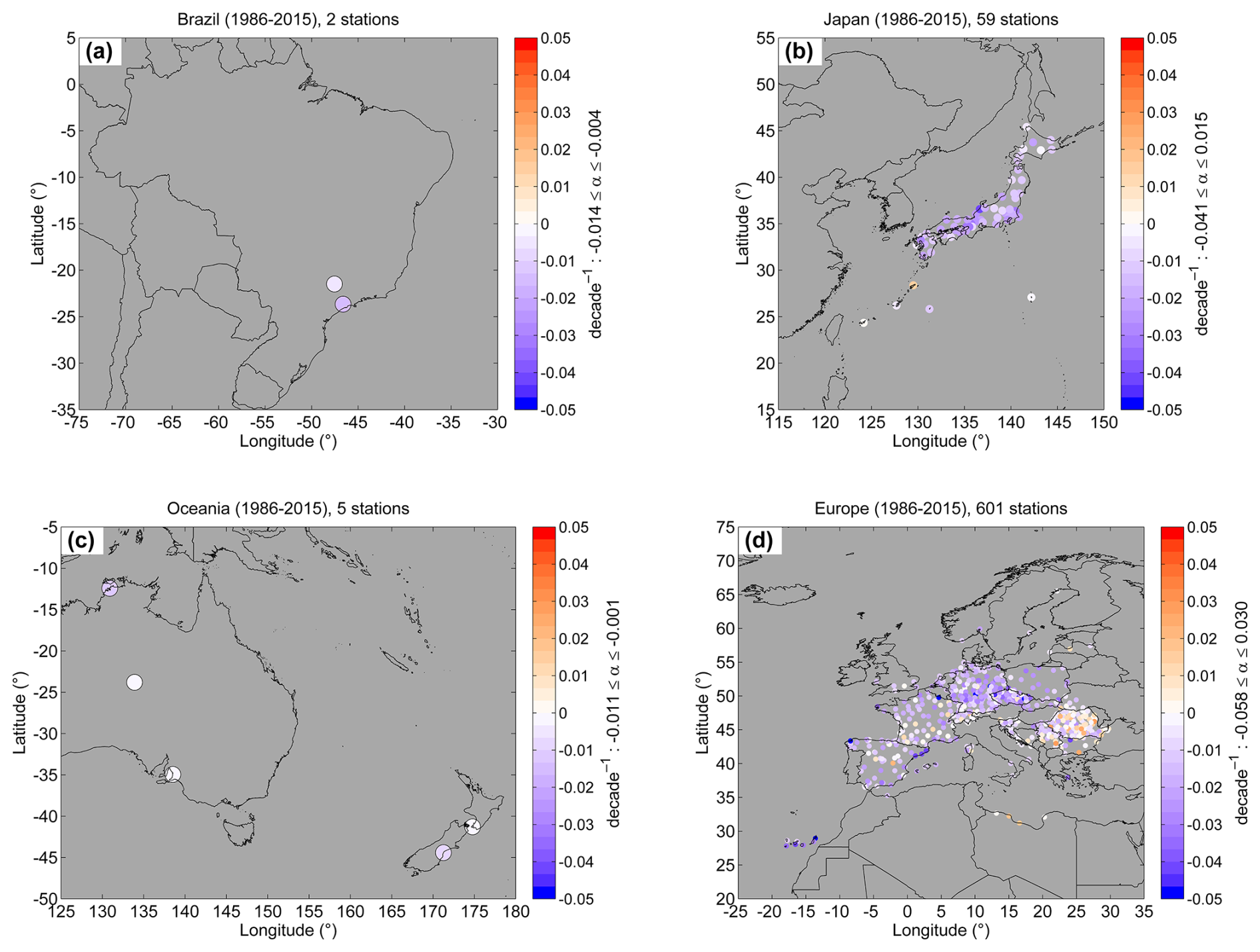
Figure 7 Spatial distribution of decadal BAOD trends based on annual means over (a) Southeast Brazil, (b) Japan, (c) Oceania, and (d) Europe for the period 1986–2015. The number of sites for each region is shown at the top. The colour–coded bar indicates the BAOD trend, whose range is indicated on the side. α represents the trend computed with DLM.

Over the 59 Japanese observational sites displayed in Fig. 7b, the decadal trends vary from (−0.041 ± 0.004) per decade (in Kanazawa) to (+0.015 ± 0.010) per decade (in Naze). Remarkably, 52 sites out of 59 exhibit significant trends. Visually, the main features appear similar when using all sites or only those with significant trends. With a national trend of (−0.015 ± 0.002) per decade, which actually started during the earlier 1960–1985 period (see Fig. 9), and 97 % of the sites having negative trends, the downward trend in BAOD is clearly established. This reveals that the air quality policies that were enacted during the earlier period had effectively resulted in a significant reduction in air pollution.

Over Oceania (Fig. 7c), the trend values vary from (−0.011 ± 0.009) decade⁻¹ (in Darwin) to (−0.001 ± 0.001) per decade (in Adelaide). As also seen in Fig. 6, the strongest negative trend is found at Darwin. Because it is the Oceania site closest to Mount Pinatubo, its trend appears to be mainly a result of the natural decay in volcanic aerosols that followed the 1991 eruption – the second–largest eruption of the 20th century). In contrast, Alice Springs experienced a transition from a dusty atmosphere to a cleaner and relatively dust-free period with low aerosol levels (Ekström et al., 2004; Lamb et al., 2009).

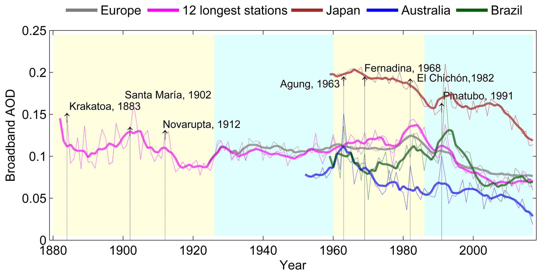
Figure 8 Overview of annual BAOD mean time series over Europe (gray line), 12 longest European stations (magenta line), Japan (brown line), Australia (blue line) and Southeast Brazil (green line). The period is from 1880 onwards.

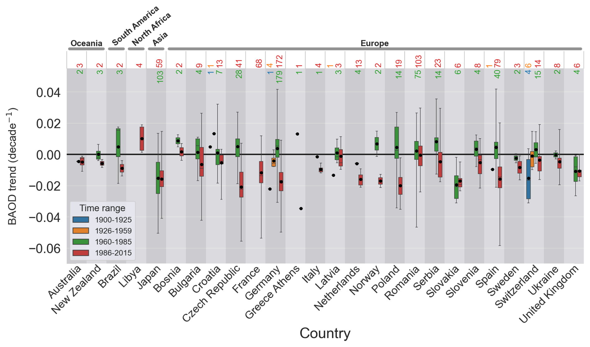
Figure 9 Box plots showing the distribution of decadal BAOD trends (y-axis) of all sites per country (x-axis) and for the four sub-periods: 1900–1925; 1926–1959; 1960–1985 and 1986–2015 in blue, brown, green, and red, respectively. The black dot shows the mean BAOD trend relative to each dataset. The number of sites per country and per period is indicated at the top of the figure. The boxes denote the 17 %–83 % range (66 % probability), and the whiskers denote the 5 %–95 % range (90 % probability) of the BAOD trends.

Figure 7d shows the BAOD trends over Europe and North Africa, including those for Switzerland, Ukraine, Latvia, and Bulgaria, based on measurements ending in 2010, 2010, 2008, and 2004, respectively. The trends fluctuate between (−0.058 ± 0.006) per decade and (+0.030 ± 0.005) per decade, averaging to a statistically significant regional trend of (−0.013 ± 0.001) per decade. A clear dominance of negative trends is observed at 85 % of stations. Nevertheless, most of the positive trends are detected over Eastern Europe, particularly in Romania, thus contrasting with other parts of Europe, as illustrated in Fig. 10. These positive trends appear to be directly related to the renewed economic development and sharp increase in accompanying aerosol emissions specific to those regions, and consistent with the Gross Domestic Product evolution (Dumitrescu et al., 2017). Overall, the European trend changed from (+0.004 ± 0.001) per decade during the 1960–1985 period to (−0.013 ± 0.001) per decade during the 1986–2015 period (see also Fig. 9). This suggests a successful recovery of the clearness of the atmosphere following air quality policies and/or some economic downturn in various regions, eventually resulting in atmospheric brightening.

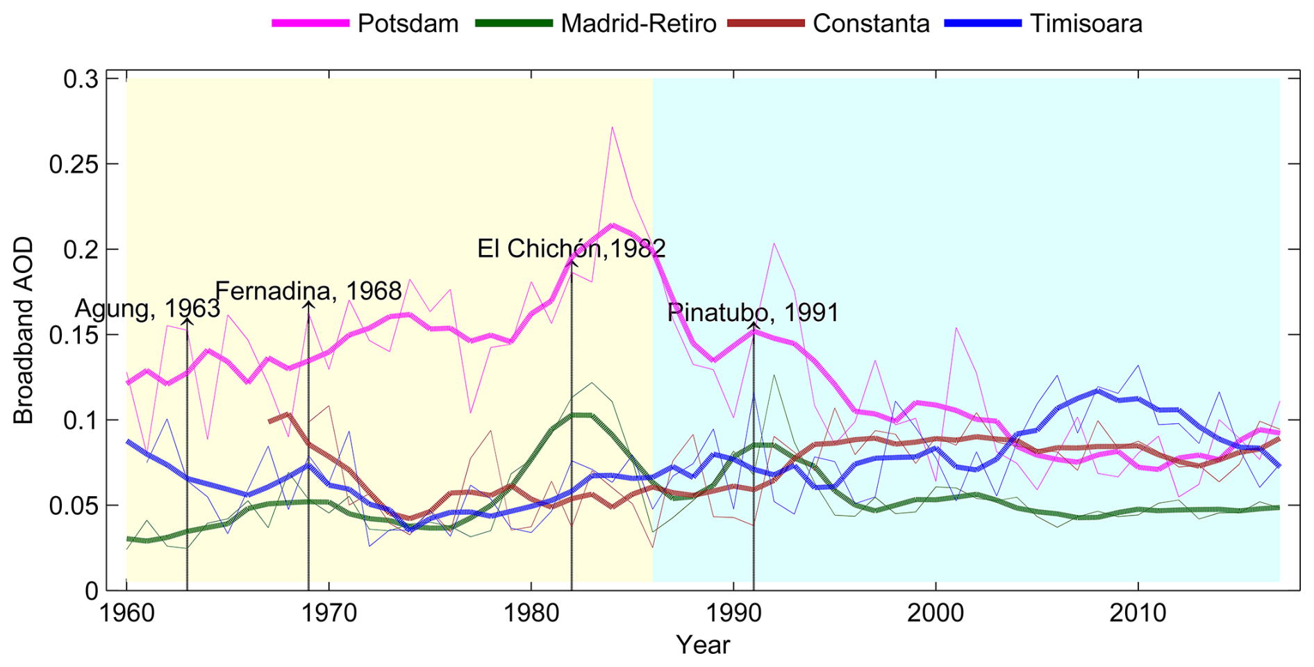
Figure 10 Annual BAOD mean time series during 1960–2015 over Potsdam (magenta), Madrid-Retiro (green line), Constanta (brown line), and Timisoara (blue line).

5 Summary and conclusions

This study has presented a reconstruction of aerosol loads dating back to the early 20th century, leveraging a novel hybrid method based on sunshine duration (SD) records and cloud observations to derive the broadband aerosol optical depth (BAOD) under cloud-free conditions. These results mark a significant advancement in the field, providing unprecedented insights into historical BAOD levels across more diverse geographical areas and extending further back in time than any prior studies.

Utilizing SD and cloudiness records, cloud-free days were carefully identified to ensure the accuracy of the derived BAOD estimates. To summarize the study's results in a combined quantitative and visual way, Fig. 11 shows the magnitude and qualitative tendencies of the annual BAOD trends over the different parts of the globe under scrutiny here, based on all the best available daily SD-derived BAOD results, including long-term observations. For each sub-period, the number of ground-based sites used to derive the corresponding regional trends is given in brackets. The blue and red arrows indicate the decline and incline of annual BAOD, respectively, for each sub-period. For Europe during 1900–1925, a decline in annual BAOD is observed at most sites, whereas a 3-time lesser decline is found during 1926–1959. Despite the considerable efforts deployed here to discover as many stations as possible during the early decades of the period under scrutiny, the observational database is considered too limited before 1960 to draw definitive conclusions regarding the global coherence and significance of the early brightening trend.

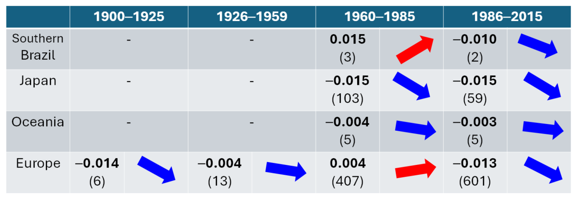
Figure 11 Changes in annual BAOD observed in different regions (first column) with noticeable site coverage during four sub-periods (from second to fifth column). For each sub-period, the numbers in bold denote the regional trend in per decade; the number of ground-based sites used to obtain the corresponding regional trend is indicated between brackets. The blue and red arrows indicate the decline or incline of annual BAOD for the sub-period.

During the 1960–1985 period, commonly described as “dimming phase”, the easternmost part of the study area – including Japan and Oceania – experienced a rapid decline in annual BAOD, especially in Japan, where the decline was ≈ 4 times faster than over Oceania. In contrast, an incline in annual BAOD occurred over both Europe and Southern Brazil, with a stronger rate in Brazil compared to Europe. During the 1986–2015 period, commonly referred to as “brightening phase”, a general decline in annual BAOD is conclusively observed over each region, with however continental variance: stronger negative trends in Brazil, Japan, and Europe compared to Oceania.

The present findings agree with earlier results related to the dimming and brightening periods that occurred across Europe, thus confirming the role of aerosols over that continent. Notably, this analysis also revealed contrasting trends in other world regions, such as Japan, where an unexpected decrease in AOD was observed during the anticipated dimming period. This confirms the positive effects of the air quality policies that were enacted there from 1960 onwards and emphasizes the regional nature of the dimming/brightening phenomenon.

For Europe, this study has contributed novel knowledge about the spatial and temporal evolution of the aerosol regime during the decades preceding 1960, when solar irradiance measurements were practically non-existent. In particular, a marked decrease in aerosol load was found from 1926 to 1959, suggesting that an “early brightening” phase had occurred even earlier than previously reported. Furthermore, the reconstructed BAOD time series, incorporating seasonal and annual averages, distinctly captured the impact of major volcanic eruptions – Agung, Arena, Fernandina Island, El Chichón, and Pinatubo – across various periods, with notable effects remarkably observed at Darwin, Australia. Consequently, it can be stated that volcanic eruptions significantly impacted the regional or even global time series of aerosol loading. The second main driver is human activity through industrialization, urbanization, and economic development. A third driver, dust emissions, has been identified at Alice Springs, Australia. Unfortunately, no sufficient historical data appear to exist over regions typically impacted by biomass burning, which is also known to be a substantial driver of aerosol burden, particularly over equatorial regions.

Overall, the present investigation has clarified the long-term role of atmospheric aerosols in the dimming/brightening phenomenon, offering a new perspective on decadal aerosol load variations over diverse regions. The innovative hybrid reduction method emerged as a powerful tool for historical aerosol load reconstruction when sunshine duration and cloud cover data are available. This study paves new avenues for (i) enhancing the performance of Earth System Model (ESM) aerosols at least at regional scale where a significant number of observational sites were already used, and (ii) assessing their radiative forcing, ultimately contributing to the refinement of ESM climate change projections and reducing uncertainties in aerosol forcing.

Appendix A: Broadband direct normal irradiance (DNI) model

The broadband direct normal irradiance G_b received on a plane normal to the sunrays at ground level is computed as the extraterrestrial irradiance corrected for the actual Sun–Earth distance G_on=ε G_o multiplied by a product of five individual broadband transmittances:

$$\begin{array}{}\text{(A1)}& G_{\mathrm{b}}=\mathit{\epsilon }{G}_{\mathrm{o}}{T}_{\mathrm{R}}{T}_{\mathrm{g}}{T}_{\mathrm{o}}{T}_{\mathrm{w}}{T}_{\mathrm{a}}\end{array}$$

where $\mathit{\epsilon }=\mathrm{1}+\mathrm{0.03344}\cos (\frac{\mathrm{2}n}{\mathrm{365.2422}}-\mathrm{0.049})$ is the Sun–Earth distance correction factor (depending on the day of the year), n the day number, starting at 1 for 1 January and G_o the extra-terrestrial irradiance received on a plane normal to the Sun rays, also known as “solar constant”, assumed here to be 1367 W m⁻². Short-term variations of the solar output, caused by solar activity, are simply neglected because small (< 0.3 % according to Gueymard, 2018) compared to the other sources of uncertainty in the method.

T_R and T_g are the broadband transmittances of Rayleigh scattering and uniformly mixed gases respectively whereby the product T_RT_g is mathematically expressed as follows:

$$\begin{array}{}\text{(A2)}& T_{\mathrm{R}}{T}_{\mathrm{g}}=\left(\mathrm{1}-{\displaystyle \frac{\mathrm{0.606}{m}_{\mathrm{R}}^{\prime }}{\mathrm{6.43}+m_{\mathrm{R}}^{\prime }}}\right)(\mathrm{1}-\mathrm{0.0075}{m_{\mathrm{R}}^{\prime }}^{\mathrm{0.875}})\end{array}$$

$m_{\mathrm{R}}^{\prime }$ is the absolute, or pressure-corrected, air mass, i.e., $m_{\mathrm{R}}^{\prime }=m_{\mathrm{R}}\exp (-\frac{z_{\mathrm{o}}}{\mathrm{8430}}$), m_R is the optical air mass for Rayleigh scattering calculated by using the following mathematical equation $m_{\mathrm{R}}={\left(\cos \left({\mathit{\theta }}_{\mathrm{s}}\right)+\mathrm{0.45665}{\mathit{\theta }}_{\mathrm{s}}^{\mathrm{0.07}}(\mathrm{96.4836}-{\mathit{\theta }}_{\mathrm{s}}{)}^{-\mathrm{1.6970}}\right)}^{-\mathrm{1}}$ and θ_s solar zenith angle.

The broadband transmittance of ozone absorption T_o is defined as:

$$\begin{array}{}\text{(A3)}& T_{\mathrm{o}}=\exp (-\mathrm{0.0365}{\left(m_{\mathrm{o}}{l}_{\mathrm{o}}\right)}^{\mathrm{0.7136}})\end{array}$$

where $m_{\mathrm{o}}={\left(\cos \left({\mathit{\theta }}_{\mathrm{s}}\right)+\mathrm{268.45}{\mathit{\theta }}_{\mathrm{s}}^{\mathrm{0.5}}(\mathrm{115.420}-{\mathit{\theta }}_{\mathrm{s}}{)}^{-\mathrm{3.2922}}\right)}^{-\mathrm{1}}$ is the optical ozone mass and l_o total column amount of ozone (DU).

The broadband transmittance of water vapor absorption T_w is mathematically defined as:

$$\begin{array}{}\text{(A4)}& T_{\mathrm{w}}=\mathrm{1.0121}-\mathrm{0.11}{\left(\mathrm{0.8}{m}_{\mathrm{w}}{l}_{\mathrm{w}}+\mathrm{0.00063}\right)}^{\mathrm{0.3}}\end{array}$$

where $m_{\mathrm{w}}={\left(\cos \left({\mathit{\theta }}_{\mathrm{s}}\right)+\mathrm{0.031141}{\mathit{\theta }}_{\mathrm{s}}^{\mathrm{0.1}}(\mathrm{92.4710}-{\mathit{\theta }}_{\mathrm{s}}{)}^{-\mathrm{1.3814}}\right)}^{-\mathrm{1}}$ is the water vapor optical mass and l_w the total column amount of water vapor (cm).

The broadband transmittance of aerosol extinction (scattering and absorption) T_a is defined as:

$$\begin{array}{}\text{(A5)}& \begin{array}{rl}{T}_{\mathrm{a}}& =\exp \left(-m_{\mathrm{a}}\mathit{\beta }\left(\mathrm{0.6777}+\mathrm{0.1464}{m}_{\mathrm{a}}\mathit{\beta }\right.\right.\\ & \left.{\left.-\mathrm{0.00626}{\left(m_{\mathrm{a}}\mathit{\beta }\right)}^{\mathrm{2}}\right)}^{-\mathrm{1.3}}\right)=\exp (-m_{\mathrm{a}}\mathrm{BAOD})\end{array}\end{array}$$

where m_a=m_w is the aerosol optical mass and β the aerosol optical depth at 1000 nm. BAOD is the broadband aerosol optical depth and can be considered approximately equal to AOD at 750 nm (Qiu, 1998; Molineaux et al., 1998).

Appendix B: Practical implementation of methodology for computing long-term trends in reconstructed atmospheric aerosol load based on large-scale sunshine duration records since 1900

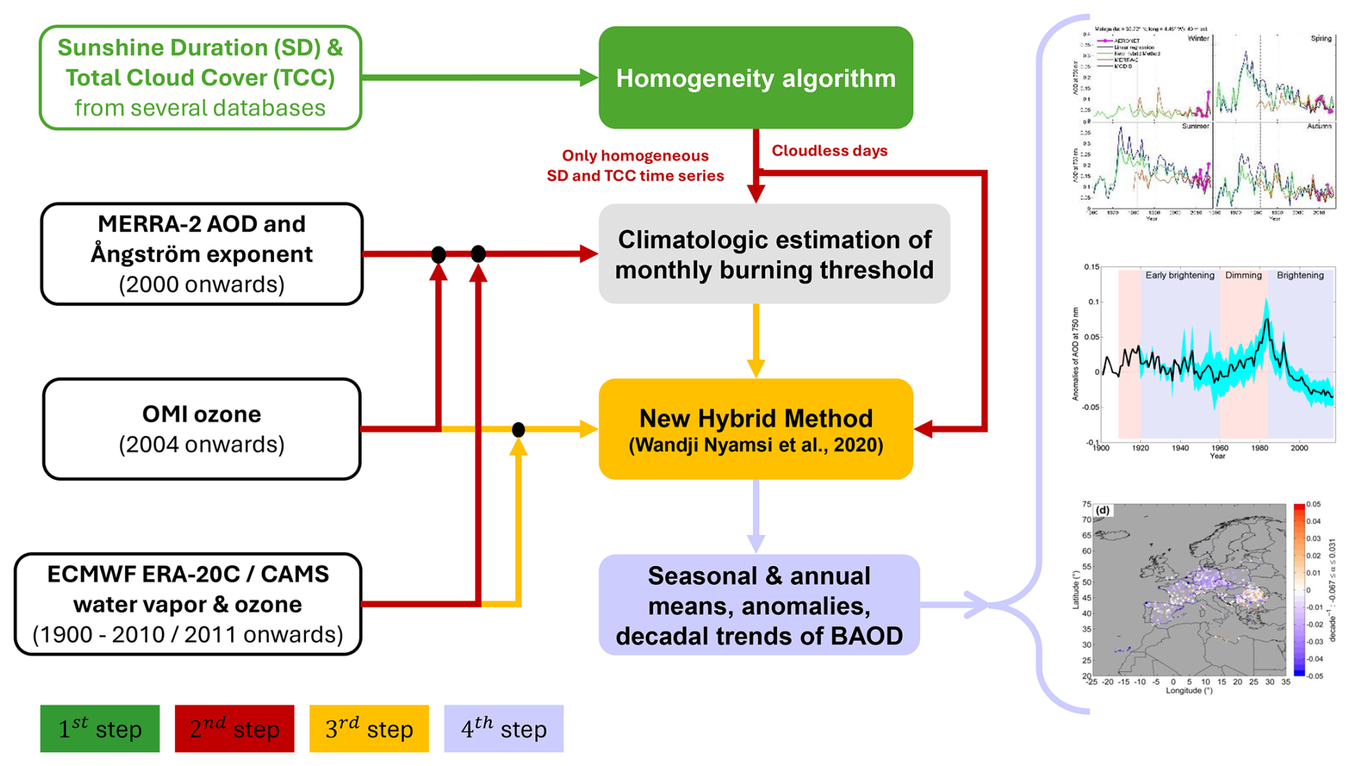
Figure B1 Sketch for computing long-term trends in reconstructed atmospheric aerosol load based on large-scale sunshine duration records since 1900.