Spatiotemporal optimization of NO_x and VOC emissions using a hybrid inversion framework and implications for ozone sensitivity-regime diagnosis

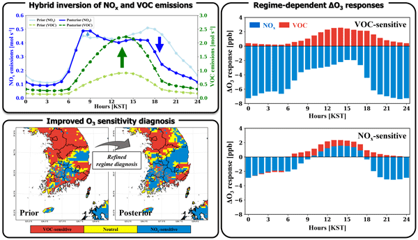
Ozone (O₃) over South Korea has risen in recent years, underscoring the need to accurately quantify emissions of nitrogen oxides (NO_x) and volatile organic compounds (VOC). We develop a hybrid inverse modeling framework that couples the Finite Difference Mass Balance (FDMB) method with four-dimensional variational data assimilation (4D-Var) using the Community Multiscale Air Quality (CMAQ) model to jointly constrain spatiotemporal NO_x and VOC emissions over South Korea. The inversion is constrained by Tropospheric Monitoring Instrument (TROPOMI) NO₂ and HCHO columns and by surface NO₂ and O₃ concentrations from the Air Quality Monitoring Station (AQMS) network. The analysis covers 1–14 May 2022, during a month that exhibited the highest mean O₃ over the past decade. Optimized NO_x emissions exhibit strong diurnal adjustments relative to the prior (nighttime reductions up to 51 % and daytime increases up to 14 %). The joint NO_x–VOC inversion produced the best consistency with assimilated AQMS O₃ observations (Index of Agreement > 0.8). Optimized emissions shift O₃ sensitivity from VOC-sensitive to NO_x-sensitive across much of the domain, improving spatial consistency with TROPOMI-derived formaldehyde-to-NO₂ ratio diagnostics. Adjoint-based hourly ΔO₃ responses reveal distinct temporal characteristics: O₃ titration by NO_x is immediate, whereas photochemical O₃ production by VOCs requires a 1–2 h reaction time. Furthermore, reactive biogenic VOCs contribute to a slight nighttime O₃ sink under NO_x-sensitive conditions. These findings motivate hour-specific, regime-specific controls rather than uniform daily reductions. Overall, the hybrid framework improves O₃ simulations and sensitivity-regime diagnosis, enabling spatiotemporally resolved precursor emission reduction guidance for effective O₃ mitigation.

1 Introduction

Surface ozone (O₃) is a highly reactive secondary air pollutant primarily formed through complex photochemical reactions involving nitrogen oxides (NO_x ≡ NO + NO₂) and volatile organic compounds (VOC). Elevated O₃ concentrations have been associated with adverse respiratory health outcomes, including asthma and pneumonia, as well as broader impacts on air quality and ecosystem health (Gryparis et al., 2004; Turner et al., 2016; Raza et al., 2018). In recent years, a persistent increase in O₃ levels has been observed across East Asia, leading to a growing demand for scientific investigation into its underlying causes. Previous studies have attributed this increase to multiple factors, including changes in atmospheric circulation patterns due to climate change, enhanced stratosphere–troposphere exchange, and shifts in the O₃ sensitivity regime (Lee et al., 2021; Itahashi et al., 2022; Hou et al., 2023).

Among these factors, shifts in the O₃ sensitivity regime play a key role in understanding the causes of rising recent O₃ levels. The O₃ sensitivity regime refers to the relative responsiveness of O₃ formation to changes in its precursor emissions, primarily NO_x and VOC. In a VOC-sensitive regime, O₃ production increases when VOC emissions rise, but shows little change or may even increase when NO_x emissions are reduced. Conversely, in a NO_x-sensitive regime, O₃ formation responds strongly to reductions in NO_x emissions. Several recent studies have reported that many regions in East Asia are currently undergoing a transition from a VOC-sensitive regime toward a transitional or NO_x-sensitive regime, while, during this transition, many regions remain sufficiently VOC-sensitive that reductions in NO_x emissions can result in increased O₃ concentrations (Lee et al., 2021; Itahashi et al., 2022; Wang et al., 2025). Accordingly, the formulation of effective O₃ mitigation strategies necessitates accurate characterization of region-specific sensitivity regimes, which in turn requires an accurate spatiotemporal estimation of NO_x and VOC emissions.

Emission estimates are typically derived using either bottom-up or top-down approaches. The bottom-up method relies on activity data and emission factors to statistically estimate emissions. While widely used, this approach is subject to high uncertainty due to variability in emission factors, spatial heterogeneity in activity data, and the extensive time and cost required to survey all emission sources (Zhao et al., 2011; Hristov et al., 2017; Solazzo et al., 2021). To overcome these limitations, top-down approaches based on inverse modeling have become increasingly prevalent. These methods assimilate satellite and ground-based observational data with chemical transport models to infer emissions that are consistent with observed atmospheric concentrations (Miller et al., 2014; Cheng et al., 2021). Various inverse modeling techniques have been applied, including mass balance (Lamsal et al., 2011; Cooper et al., 2017; Li et al., 2019; Qu et al., 2019; Momeni et al., 2024), four-dimensional variational data assimilation (4D-Var) (Hu et al., 2022, 2023; Voshtani et al., 2023; Nüß et al., 2025), and ensemble Kalman filter (EnKF) methods (Peng et al., 2017; Jia et al., 2022; Wu et al., 2023). The mass balance approaches are computationally efficient and suitable for rapid emission updates, but are known to be susceptible to smearing effects due to pollutant transport (Cooper et al., 2017). Among the mass balance-based methods, the Finite Difference Mass Balance (FDMB) method has been shown to improve emission estimates by exploiting sensitivities between emissions and column concentrations (Cooper et al., 2017; Mun et al., 2023). In contrast, the 4D-Var approach uses adjoint sensitivity to trace the influence of emission sources backward in time, thereby reducing transport-induced smearing errors (Li et al., 2019). However, it is computationally intensive and requires the development of an adjoint model, which can be a substantial limitation. To leverage the strengths of both approaches, a hybrid inverse modeling framework combining the mass balance and the 4D-Var has been recently applied (Qu et al., 2017, 2019; Chen et al., 2021; Choi et al., 2022; Moon et al., 2024).

Accurately reproducing O₃ concentrations remains a critical challenge due to its short-lived and chemically reactive nature. Because diurnal variations in precursor emissions strongly influence O₃ formation through nonlinear photochemical processes (Wang et al., 2018), it is essential to simultaneously capture the hourly evolution of emissions and constrain the relative contributions of both NO_x and VOCs. Therefore, a comprehensive inverse modeling framework capable of simultaneously optimizing the spatiotemporal distribution of both precursor emissions is required.

In this study, we develop a hybrid inverse modeling framework that combines the FDMB and 4D-Var methods with the Community Multiscale Air Quality (CMAQ) model to simultaneously constrain the spatiotemporal distributions of NO_x and VOC emissions over South Korea, to improve O₃ simulations and sensitivity regime diagnostics, and to quantify hourly ΔO₃ responses to NO_x and VOC emissions using adjoint sensitivities. Here, ΔO₃ represents the change in O₃ concentration in response to changes in precursor emissions, as diagnosed by the adjoint model. The inverse modeling system is constrained using satellite-based measurements from the TROPOspheric Monitoring Instrument (TROPOMI) and in situ observations from the Air Quality Monitoring Station (AQMS) network. We further analyze the changes in O₃ concentrations and O₃ sensitivity regimes before and after inverse modeling to propose a robust top-down emission adjustment approach that can inform the development of future O₃ mitigation policies. The results are presented in four sections: (1) spatiotemporal corrections in emissions (Sect. 3.1), (2) spatiotemporal corrections in NO₂, HCHO, and O₃ concentrations (Sect. 3.2), (3) improvement of O₃ sensitivity regimes through hybrid inversion (Sect. 3.3), and (4) regime-dependent hourly ΔO₃ responses to NO_x and VOC emissions (Sect. 3.4).

2 Methods

2.1 WRF/CMAQ modeling system

In this study, we employed version 5.0 of the Community Multiscale Air Quality (CMAQ) model, developed by the U.S. Environmental Protection Agency (EPA), which includes an adjoint model, to conduct 4D-Var inverse modeling (Zhao et al., 2020a). Meteorological input fields required for the CMAQ simulation were generated using the Weather Research and Forecasting (WRF) model version 3.8.1 (Skamarock et al., 2008). The modeling domains consisted of two nested grids: a coarse-resolution outer domain (D1) covering East Asia at a horizontal resolution of 27 km and a finer-resolution inner domain (D2) focusing on South Korea at 9 km resolution (Fig. 1).

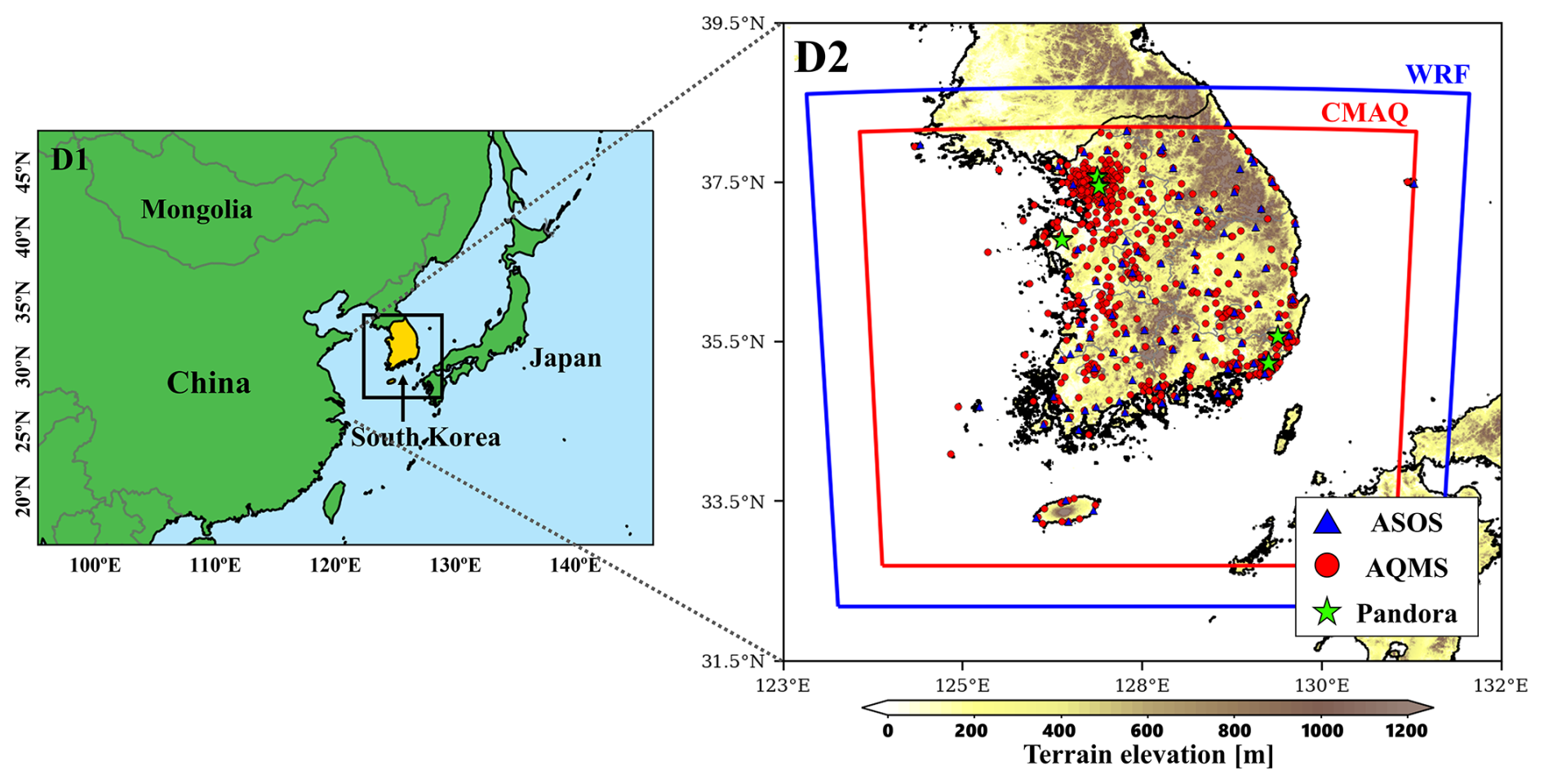
Figure 1 WRF/CMAQ modeling domains and spatial distribution of observational sites (ASOS: blue triangles; AQMS: red circles; Pandora: green stars).

This study targeted South Korea, and the inverse modeling was conducted exclusively over D2. The initial and boundary conditions for the WRF simulation were obtained from the ERA5 reanalysis dataset with a spatial resolution of 0.25° × 0.25°, provided by the European Centre for Medium-Range Weather Forecasts (ECMWF) (Hersbach et al., 2023a, b). To improve the accuracy of meteorological fields, grid nudging was applied during WRF simulations (Jeon et al., 2015).

We utilized the Emissions Database for Global Atmospheric Research-Hemispheric Transport of Air Pollution version 3 (EDGAR-HTAPv3) as the source of anthropogenic emissions. This inventory incorporates national emission estimates from South Korea's Clean Air Policy Support System (CAPSS) and provides monthly averaged emissions at a spatial resolution of 0.1° × 0.1° for nine key air pollutants: black carbon (BC), carbon monoxide (CO), nitrogen oxides (NO_x), sulfur dioxide (SO₂), ammonia (NH₃), organic carbon (OC), non-methane volatile organic compounds (NMVOC), particulate matter with an aerodynamic diameter ≤ 10 µm (PM₁₀), and particulate matter with an aerodynamic diameter ≤ 2.5 µm (PM_2.5) (Crippa et al., 2023). To generate the hourly gridded emissions required for CMAQ modeling, the monthly data were temporally downscaled using sector-specific temporal allocation profiles (Crippa et al., 2020). In addition, biogenic volatile organic compound (BVOC) emissions, which serve as key precursors of O₃, were estimated using the Model of Emissions of Gases and Aerosols from Nature (MEGAN) version 2.1 (Guenther et al., 2012).

The CMAQ simulations were conducted from 27 April to 15 May 2022, including a 4 d spin-up period. The analysis focuses on 1–14 May 2022 (two weeks), selected for computational efficiency during the month that recorded the highest monthly average surface O₃ concentrations over South Korea in the past decade (Fig. S1 in the Supplement). Detailed model configurations for both WRF and CMAQ are provided in Tables S1 and S2 in the Supplement. Initial and boundary conditions for the outer domain (D1) were derived from default CMAQ vertical profile data, while the inner domain (D2) was driven by D1 through one-way nesting.

2.2 Observation data

2.2.1 Ground-based observations

For the evaluation of meteorological and air quality model performance and the implementation of inverse modeling over South Korea, we utilized ground-based observational data from Automated Surface Observing System (ASOS), Air Quality Monitoring Stations (AQMS), and Pandora spectrometers (Fig. 1). Hourly measurements of temperature, wind speed, and relative humidity from 95 ASOS sites were used to assess the accuracy of meteorological simulations. For air quality model evaluation and inverse modeling, hourly NO₂ and O₃ concentrations from 619 AQMS sites were used. In the baseline inversion, all sites were used for both data assimilation and evaluation. To assess the robustness of the posterior emissions using independent observations, an additional validation experiment was conducted using a data-splitting approach, in which 496 sites (80 %) were randomly selected for the inversion and the remaining 123 sites (20 %) were reserved for independent validation. The spatial distribution of the selected sites is shown in Fig. S2.

In addition, tropospheric NO₂ and HCHO Vertical Column Densities (VCDs) were obtained from Pandora spectrometers at five sites operated by the Pandonia Global Network (PGN) to evaluate the model's performance in simulating NO_x and VOC-related column concentrations. To ensure data reliability, only Pandora NO₂ retrievals with Level 2 (L2) data quality flags classified as “high” quality (flags 0 and 10) were used. For HCHO, L2 retrievals classified as “high” quality (flags 0 and 10) or “medium” quality (flags 1 and 11) were used in this study (Bae et al., 2025; Fu et al., 2025). The Pandora observations were hourly averaged for comparison with model results.

2.2.2 TROPOMI NO₂ and HCHO observations

TROPOMI is the single payload aboard the European Space Agency (ESA)'s Sentinel-5 Precursor (S5P) satellite, launched on 13 October 2017 (Veefkind et al., 2012). Operating in a sun-synchronous polar orbit at an altitude of approximately 800 km, it provides daily global coverage with a high spatial resolution footprint of 5.5 km × 3.5 km at nadir and an equator crossing time near 13:30 local solar time.

Tropospheric VCDs of NO₂ and HCHO used in this study were obtained from the TROPOMI Level 2 operational products (De Smedt et al., 2021; van Geffen et al., 2022). Both products are retrieved using a three-step Differential Optical Absorption Spectroscopy (DOAS) technique: (1) fitting of the Slant Column Density (SCD), (2) separation of the tropospheric components from the total SCD, and (3) conversion from slant to vertical column using an air mass factor (AMF). The retrieval accuracy of VCD is highly sensitive to the a priori vertical profile used in the AMF calculation (Cooper et al., 2020). In the operational products, these profiles are derived from global simulations of the TM5-MP chemistry model at a coarse resolution of 1° × 1°, which is much coarser than the native resolution of the TROPOMI SCDs. This spatial mismatch has been linked to underestimation of VCDs, particularly over regions with strong or localized emissions (Judd et al., 2020; Douros et al., 2023; Goldberg et al., 2024).

To mitigate this limitation, we recalculate the satellite VCDs using Eq. (1) (Souri et al., 2016), which adjusts the satellite-derived VCDs (VCD_satellite) by accounting for differences between the a priori profiles used in the satellite retrieval and those from a regional chemical transport model.

$$\begin{array}{}\text{(1)}& {\mathrm{VCD}}_{\mathrm{satellite}}^{\prime }={\displaystyle \frac{{\mathrm{VCD}}_{\mathrm{satellite}}\times {\mathrm{AMF}}_{\mathrm{satellite}}}{{\mathrm{AMF}}_{\mathrm{model}}}}\end{array}$$

AMF_satellite is the AMF provided in the TROPOMI Level 2 product, and AMF_model is a model-derived AMF calculated using the vertical profile from the CMAQ model and the TROPOMI Averaging Kernel (AK) (Eq. 2). Here, AMF_apriori denotes the a priori air mass factor provided in the TROPOMI Level 2 product, which is used as the reference AMF in the satellite retrieval.

$$\begin{array}{}\text{(2)}& {\mathrm{AMF}}_{\mathrm{model}}={\mathrm{AMF}}_{\mathrm{apriori}}{\displaystyle \frac{\sum \mathrm{AK}\times {\mathrm{VCD}}_{\mathrm{model}}}{\sum {\mathrm{VCD}}_{\mathrm{model}}}}\end{array}$$

To ensure data quality, we applied a quality assurance threshold of qa_value > 0.75 for NO₂ (high quality), which is relaxed to >0.5 for HCHO (moderate quality) to retain sufficient sampling.

2.3 Inverse modeling

2.3.1 Finite Difference Mass Balance inversion using 3D-Var

The mass balance approach estimates emissions by assuming a linear relationship between observed column concentrations and surface emissions (Cooper et al., 2017). Among the mass balance-based methods, the Finite Difference Mass Balance (FDMB) method, proposed by Lamsal et al. (2011), introduces a scaling factor (β) to account for nonlinear relationships between changes in column concentrations (ΔΩ) and emissions (ΔE) (Eqs. 3 and 4). Here, ΔΩ_m represents the change in modeled column concentrations in response to a prescribed perturbation in emissions, while ΔE_m denotes the imposed emission perturbation used to estimate the sensitivity. In this study, ΔE_m is defined by a 10 % perturbation of the prior emissions.

$$\begin{array}{}\text{(3)}& {\displaystyle }{E}_{\mathrm{FDMB}}=E_{\mathrm{m}}\left(\mathrm{1}+{\displaystyle \frac{{\mathrm{\Omega }}_{\mathrm{a}}-{\mathrm{\Omega }}_{\mathrm{m}}}{\mathit{\beta }{\mathrm{\Omega }}_{\mathrm{m}}}}\right)\text{(4)}& {\displaystyle }\mathit{\beta }={\displaystyle \frac{\mathrm{\Delta }{\mathrm{\Omega }}_{\mathrm{m}}/{\mathrm{\Omega }}_{\mathrm{m}}}{\mathrm{\Delta }{E}_{\mathrm{m}}/{\mathrm{E}}_{\mathrm{m}}}}\end{array}$$

Here, E_FDMB represents the FDMB emissions, E_m is the a priori model emissions, Ω_a is the analysis field used as the observational constraint, and Ω_m is the simulated column density from the prior simulation. The sensitivity factor β is calculated from the prior simulation and a perturbed simulation in which emissions are increased by 10 %. The β value is constrained between 0.1 and 10 to prevent unrealistic corrections (Cooper et al., 2017; Li et al., 2019; Mun et al., 2023).

In this study, we applied the FDMB inversion to constrain NO_x and VOC emissions. To mitigate potential inversion errors arising from the highly non-linear dependence of HCHO production on background NO_x concentrations (Wolfe et al., 2016), we sequenced the initial mass-balance step by optimizing NO_x prior to VOCs. Specifically, we first derived an emission factor for NO_x based on the sensitivity of NO₂ columns to NO_x emissions (Eq. 5). Establishing this updated NO_x baseline in the forward model effectively reduces the non-linearities associated with HCHO yields. Following this, we corrected VOC emissions using HCHO columns as observational constraints. For this step, total VOC emissions were separated into anthropogenic (AVOC) and biogenic (BVOC) categories, as their distinct species compositions lead to different HCHO responses (Millet et al., 2006; Choi et al., 2022; Oomen et al., 2024). We independently quantified the HCHO column sensitivities to AVOC and BVOC emissions (Eqs. 6 and 7). Based on these sensitivities, we derived emission factors for both AVOC and BVOC components.

$$\begin{array}{}\text{(5)}& {\displaystyle }{\mathit{\beta }}_{{\mathrm{NO}}_x}={\displaystyle \frac{\mathrm{\Delta }{\mathrm{\Omega }}_{{\mathrm{NO}}_{\mathrm{2}}}/{\mathrm{\Omega }}_{{\mathrm{NO}}_{\mathrm{2}}}}{\mathrm{\Delta }{E}_{{\mathrm{NO}}_x}/E_{{\mathrm{NO}}_x}}}\text{(6)}& {\displaystyle }{\mathit{\beta }}_{\mathrm{AVOC}}={\displaystyle \frac{\mathrm{\Delta }{\mathrm{\Omega }}_{\mathrm{HCHO}}/{\mathrm{\Omega }}_{\mathrm{HCHO}}}{\mathrm{\Delta }{E}_{\mathrm{AVOC}}/E_{\mathrm{AVOC}}}}\text{(7)}& {\displaystyle }{\mathit{\beta }}_{\mathrm{BVOC}}={\displaystyle \frac{\mathrm{\Delta }{\mathrm{\Omega }}_{\mathrm{HCHO}}/{\mathrm{\Omega }}_{\mathrm{HCHO}}}{\mathrm{\Delta }{E}_{\mathrm{BVOC}}/E_{\mathrm{BVOC}}}}\end{array}$$

However, traditional mass balance approaches may incorporate biases inherent in satellite observations into the inferred emission estimates. While iterative applications of the mass balance method can theoretically reduce spatial smearing errors, localized scaling factors become highly vulnerable to overfitting this observational noise when applied at fine model resolutions, such as our 9 km grid. A pseudo-observation test conducted by Moon (2025) demonstrated that iterating the FDMB framework at this high resolution increased emission errors due to the propagation of residual noise through repeated updates. To address these challenges associated with observational uncertainties and noise propagation, we incorporated a 3D-Var data assimilation step into our framework to generate a smoothed analysis field as the observational constraint for the FDMB inversion. In this configuration, the 3D-Var step serves as an observational constraint that provides chemically and physically consistent constraints to mitigate error propagation into the top-down emission fields (East et al., 2022), allowing the FDMB inversion to establish a robust spatial baseline (Fig. 2).

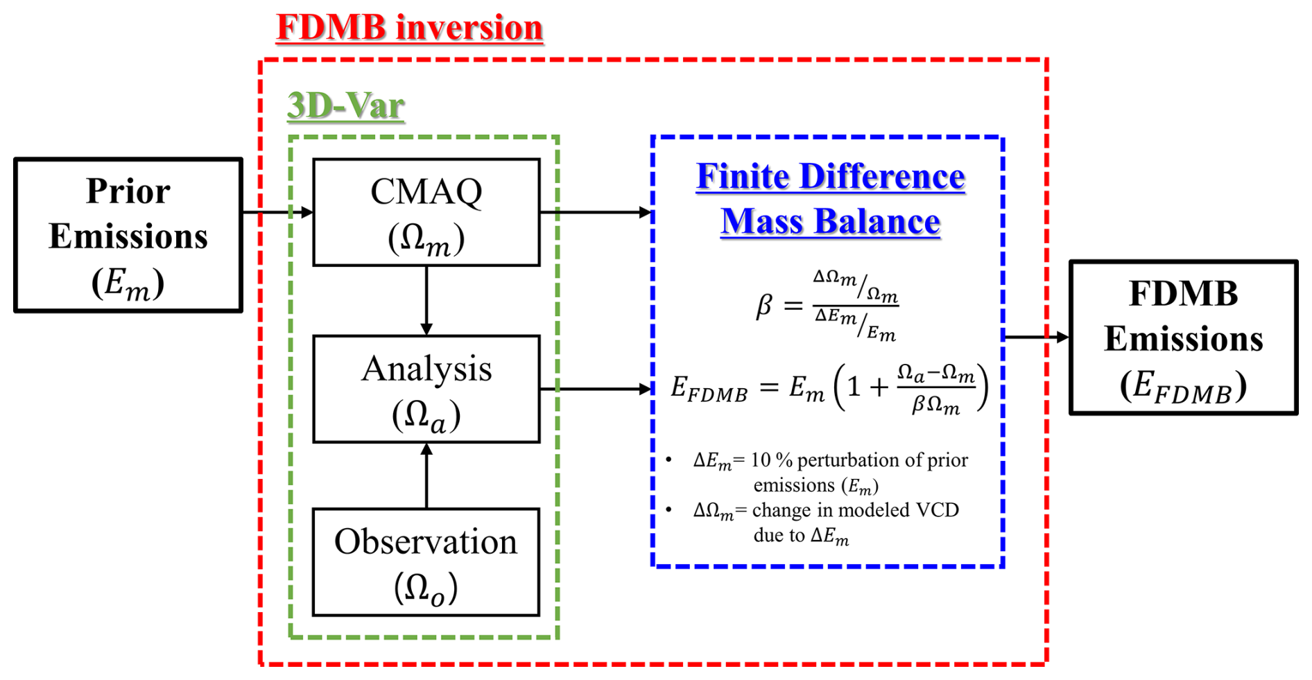
Figure 2 Flowchart of the FDMB inversion framework with 3D-Var assimilation. The red dashed box denotes the overall FDMB inversion framework, the green dashed box represents the 3D-Var assimilation step (Ω_m: CMAQ VCD, Ω_o: observed VCD, Ω_a: analysis VCD), and the blue dashed box indicates the finite-difference mass balance step used to update emissions based on finite-difference sensitivities.

Furthermore, to minimize errors associated with transport-induced smearing, the FDMB inversion was performed using two-week-averaged column densities for both the model and observations over the study period, following previous studies (Lamsal et al., 2011; Chen et al., 2021; Mun et al., 2023). Consequently, this study focused on constraining the spatial distribution of emissions based on temporally averaged observations, without accounting for temporal variability in emissions. While the FDMB method can theoretically be extended to separate time windows, the once-daily overpass of TROPOMI inherently limits its capacity to independently resolve diurnal temporal variability. Therefore, the FDMB step is used strictly to establish a robust spatial baseline, while hourly variations are optimized in the subsequent 4D-Var inversion.

2.3.2 4D-Var inversion

While the FDMB inverse modeling enables spatial correction of emissions effectively, it cannot account for their temporal variability. To overcome this limitation, we implemented a four-dimensional variational (4D-Var) inversion approach to constrain the spatial and temporal distribution of emissions. The cost function employed in this study is defined in Eq. (8).

$$\begin{array}{}\text{(8)}& \begin{array}{rl}J\left(\mathit{\alpha }\right)& ={\displaystyle \frac{\mathrm{1}}{\mathrm{2}}}\mathit{\gamma }\sum _{i=\mathrm{0}}^{n-\mathrm{1}}{\left({\mathit{\alpha }}_i-{\mathit{\alpha }}_b\right)}^T{B}_i^{-\mathrm{1}}\left({\mathit{\alpha }}_i-{\mathit{\alpha }}_b\right)\\ & +{\displaystyle \frac{\mathrm{1}}{\mathrm{2}}}\sum _{i=\mathrm{1}}^n{\left(y_i-H_i\left(c_i\right)\right)}^T{R}_i^{-\mathrm{1}}\left(y_i-H_i\left(c_i\right)\right),\\ & \text{where}{c}_i=M_{i-\mathrm{1}\to i}\left(c_{i-\mathrm{1}}{e}_{i-\mathrm{1}}\right)\end{array}\end{array}$$

Here, n represents the number of hourly time steps within the assimilation window, which was set to 24 in this study. The control variable is the emission scaling factor (α_i) at a specific hourly time step i ($i=\mathrm{0},\mathrm{\dots },n-\mathrm{1})$. The emission scaling factor (${\mathit{\alpha }}_i=e_i/e_i^b$) represents the ratio between the updated emissions (e_i) and the prior emissions ($e_i^b$).

c_i represents the simulated concentration field at time step i. As explicitly denoted by the forward model integration operator $M_{i-\mathrm{1}\to i}$, the concentration field c_i is obtained by integrating the model from time step i−1 to i using the previous concentration field c_i−1 and emissions e_i−1. Because c_i−1 already contains the accumulated effects of earlier emissions, transport, chemical reaction, and initial conditions, c_i reflects the cumulative atmospheric history up to time step i rather than the influence of e_i−1 alone. Consequently, to appropriately account for the transport and chemical processing time in the adjoint backward integration, the observation term is evaluated from i=1 to n, corresponding to the concentrations driven by emissions from i=0 to n−1. y_i denotes the observation vector at time step i, consisting of hourly AQMS NO₂ and O₃ concentrations, and H_i denotes the observation operator that maps the model concentration field c_i onto the corresponding AQMS observation space. Thus, the observation term compares hourly AQMS observations with the simulated concentrations mapped to the corresponding station locations and times, rather than comparing observations directly with emissions.

B_i and R_i are the error covariance matrices for emission scaling factors and observations, respectively. Assuming spatial independence, both B_i and R_i were configured as diagonal matrices. The prior uncertainty for the emissions was set to 100 %, which corresponds to assuming a standard deviation of 1.0 for the prior emission scaling factors (α_b=1). Consequently, the corresponding variance is 1.0, and the diagonal elements of B_i were set to 1.0. Under this Gaussian error assumption, the background penalty term is symmetrically evaluated; for instance, a doubling of emissions (α_i=2) and a complete zeroing of emissions (α_i=0) incur the same mathematical penalty in the cost function.

For ground-based AQMS observations, the total observational error was estimated as the sum of measurement errors (ϵ_o) and representativeness errors (ϵ_r), such that ${\mathit{ϵ}}_{\mathrm{tot}}=\sqrt{{\mathit{ϵ}}_{\mathrm{o}}^{\mathrm{2}}+{\mathit{ϵ}}_{\mathrm{r}}^{\mathrm{2}}}$ (Elbern et al., 2007; Feng et al., 2018). Specifically, ϵ_o is defined as ${\mathit{ϵ}}_{max}+\mathrm{0.0075}\times y_{\mathrm{obs}}$, where ϵ_max is a base error limit set to 1.5 µg m⁻³ for both NO₂ and O₃, and y_obs is the observed concentration. The representativeness error (ϵ_r) is parameterized as ${\mathit{ϵ}}_{\mathrm{r}}=\mathit{\kappa }\sqrt{\mathrm{\Delta }x/L}$, where κ is a tunable scaling factor (0.5), Δx is the grid spacing (9 km), and L represents the radius of influence of an observation (set to 3 km).

In this study, the assimilation time window was set to 24 h to better represent diurnal variations in atmospheric processes. To prevent overfitting or underfitting in the inversion process, a regularization parameter γ was introduced (Henze et al., 2009; Chen et al., 2021; Yu et al., 2021), and its optimal value was determined using the L-curve test (Hansen, 1999). The optimized γ was then used to constrain the spatiotemporal distribution of emissions, ensuring physically realistic corrections.

2.3.3 Hybrid inverse modeling framework

In this study, we applied the hybrid inverse modeling framework proposed by Moon et al. (2024) to constrain the spatiotemporal distribution of NO_x and VOCs, which are key precursors influencing O₃ formation and destruction. The hybrid inverse modeling approach consists of a two-step process: an initial adjustment of the spatial distribution of emissions using the FDMB method, followed by a refinement of the spatiotemporal distribution through 4D-Var inverse modeling. A model-based twin experiment by Moon et al. (2024) demonstrated that a standalone 4D-Var approach structurally struggles to effectively correct emissions in grid cells with exceptionally large prior spatial errors. By sequentially combining these methods, the FDMB step establishes a robust and accurate spatial baseline, which enables the subsequent 4D-Var step to focus more effectively on optimizing diurnal temporal variations and multi-species chemical feedbacks, while reducing the influence of spatial distribution errors in the prior emissions. While the original framework primarily focused on single-species corrections such as NO₂, we extended the approach to jointly optimize both NO_x and VOC emissions to better represent the nonlinear photochemical processes governing O₃ formation. A schematic of the hybrid inverse modeling framework is shown in Fig. 3.

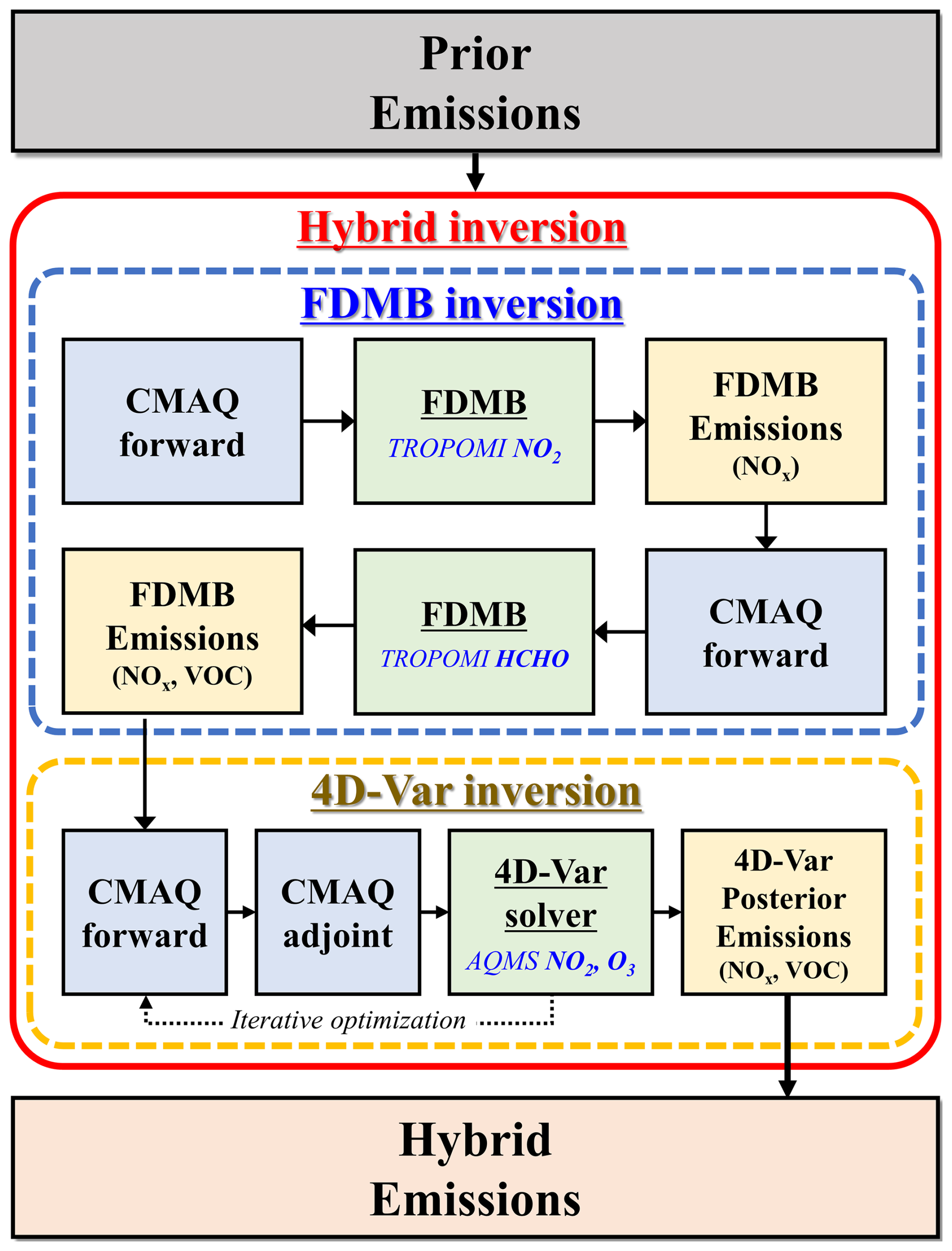
Figure 3 Schematic of the hybrid inverse modeling framework combining FDMB and 4D-Var inversions. In the first step, the FDMB inversion (blue box) corrects the spatial distribution of NO_x and VOC emissions using TROPOMI NO₂ and HCHO VCDs. In the second step, the 4D-Var inversion (yellow box) constrains the spatiotemporal distribution of NO_x and VOC emissions by assimilating hourly ground-based NO₂ and O₃ observations.

The prior emissions used in this study are derived from the EDGAR-HTAPv3 inventory, temporally disaggregated to hourly resolution using sector-specific temporal allocation profiles (Crippa et al., 2020). First, we performed FDMB inversions for NO_x and VOC emissions in two sequential steps. In the first step, TROPOMI NO₂ VCDs were used to update the spatial distribution of NO_x emissions. In the second step, TROPOMI HCHO VCDs were utilized to correct VOC emissions. Given the different source characteristics of VOC, we estimated separate scaling factors for AVOC and BVOC. As the FDMB inversion relies on two-week-averaged satellite column observations, it corrects only the spatial distribution of emissions without modifying their temporal allocation.

Next, the FDMB NO_x and VOC emissions were used as the prior estimate for a 4D-Var inversion. In this step, we assimilated hourly NO₂ and O₃ measurements from the AQMS network, which are highly sensitive to changes in NO_x and VOC emissions. The control variables in the 4D-Var system included both NO_x and 15 VOC species (Table S3), enabling the joint optimization of key precursors that drive O₃ formation and variability. The 4D-Var inversion was applied sequentially using a 24 h assimilation window over the two-week analysis period, with the FDMB-corrected emissions serving as the spatial prior for each window. The optimized concentration fields from each window were carried over as initial conditions for the subsequent day's forward integration, allowing the atmospheric state to evolve continuously across the analysis period.

To evaluate the effectiveness of the hybrid inverse modeling approach, we designed three experiments: (1) Prior, which used anthropogenic emissions from the EDGAR-HTAPv3 inventory and biogenic VOC emissions from MEGAN v2.1; (2) Hybrid_NOx, which corrected only NO_x emissions; and (3) Hybrid_NOx+VOC, which jointly constrained NO_x and VOC emissions. By comparing the model outputs from all three experiments with ground-based observations, including AQMS NO₂ and O₃ concentrations and Pandora NO₂ and HCHO VCDs, and by using TROPOMI NO₂ and HCHO columns for satellite-based O₃ sensitivity-regime diagnostics, we assessed the effects of NO_x and VOC emission constraints on the spatiotemporal distribution of O₃ and its sensitivity regime. Model performance was assessed using multiple statistical metrics (Table S4).

2.4 O₃ sensitivity regime classification

The O₃ sensitivity regime can be classified based on the $\mathrm{VOC}/{\mathrm{NO}}_x$ ratio, for which several photochemical indicators – such as $\mathrm{HCHO}/{\mathrm{NO}}_{\mathrm{2}}$, ${\mathrm{H}}_{\mathrm{2}}{\mathrm{O}}_{\mathrm{2}}/{\mathrm{HNO}}_{\mathrm{3}}$, and ${\mathrm{H}}_{\mathrm{2}}{\mathrm{O}}_{\mathrm{2}}/{\mathrm{NO}}_y$ – have been widely applied (Sillman, 1995; Liu and Shi, 2021). Among these, the HCHO-to-NO₂ ratio has been widely used because it is applicable to satellite observations and can effectively capture regional-scale photochemical conditions (Duncan et al., 2010; Liu et al., 2021; Jang et al., 2023; Rahman et al., 2025). In this study, we assess the model's capability to diagnose O₃ sensitivity regimes by comparing HCHO-to-NO₂ ratios derived from TROPOMI satellite measurements with those simulated by the model. Conventionally, we classified HCHO-to-NO₂ ratios ≤ 2.0 as VOC-sensitive, ≥ 2.8 as NO_x-sensitive, and between 2.0 and 2.8 as neutral, following the thresholds proposed by Jang et al. (2023) for South Korea.

2.5 Adjoint-based analysis of ΔO₃ responses to precursor emissions

We quantified the hourly influence of NO_x and VOC emissions on O₃ as a function of the sensitivity regime using the CMAQ adjoint model. The primary objective of this analysis is to identify how emissions released at different hours contribute to O₃ concentrations at specific times of the day, thereby resolving the diurnal characteristics of precursor–O₃ relationships under different sensitivity regimes. To this end, a forward CMAQ simulation was first performed using the posterior emissions from the Hybrid_NOx+VOC experiment to generate the concentration fields required for adjoint integration. The adjoint model was then driven by these concentration fields, with a separate diagnostic cost function J_Reg(h_r) defined for each local hour h_r – distinct from the optimization cost function J(α) used in the 4D-Var inversion (Eq. 8) – as the two-week mean of the spatially averaged surface O₃ over grids classified as regime r at that hour:

$$\begin{array}{}\text{(9)}& \begin{array}{rl}& J_{\mathrm{Reg}}\left(h_r\right)={\displaystyle \frac{\mathrm{1}}{\left|D\right|}}\sum _{d\in D}{\displaystyle \frac{\mathrm{1}}{\left|G_{\mathrm{Reg}}\right|}}\sum _{g\in G_{\mathrm{Reg}}}{C}_{{\mathrm{O}}_{\mathrm{3}}}(g,h_r,d),\\ & h_r\in \left\{\mathrm{0},\mathrm{1},\mathrm{\dots },\mathrm{23}\right\},\\ & \mathrm{Reg}\in \left\{\text{VOC-sensitive},{\mathrm{NO}}_x\text{-sensitive}\right\}\end{array}\end{array}$$

Here, d denotes an individual analysis day ($d=\mathrm{1},\mathrm{2},\mathrm{\dots },\mathrm{14}$, corresponding to 1–14 May 2022), D is the complete set of 14 analysis days, g refers to an individual model grid cell, G_Reg is the set of all grid cells classified as regime Reg, and $C_{{\mathrm{O}}_{\mathrm{3}}}\left(g{h}_{r}d\right)$ is the simulated surface O₃ concentration at grid cell g, local hour h_r, and day d.

It is important to note that J_Reg(h_r) serves as a diagnostic receptor function, not as an optimization cost function subject to minimization. Unlike the 4D-Var cost function J(α) in Eq. (8), J_Reg(h_r) is not iteratively minimized; instead, it defines the O₃ indicator whose sensitivity to precursor emissions is to be quantified. Here, h_r denotes the receptor hour – the hour at which surface O₃ is evaluated as the response variable – and h_e denotes the emission hour – the hour at which precursor emissions are released and exert their influence. That is, the adjoint model quantifies how much the O₃ concentration at h_r is attributable to emissions released at each prior hour h_e. The adjoint model is initialized from J_Reg(h_r) and integrated backward in time through a single backward integration, propagating the gradient of J_Reg(h_r) through the chemical and physical processes of the model to yield sensitivities to precursor emissions at all prior emission hours h_e.

A single adjoint integration performed for a given receptor hour h_r simultaneously provides the sensitivities of J_Reg(h_r) to emissions at all emission hours h_e, defined as:

$$\begin{array}{}\text{(10)}& S_i\left(h_{\mathrm{e}}\to h_r\right)={\displaystyle \frac{\partial J_{\mathrm{Reg}}\left(h_r\right)}{\partial E_i\left(h_{\mathrm{e}}\right)}},i\in \mathit{\{}{\mathrm{NO}}_x,\mathrm{VOC}\mathit{\}}\end{array}$$

where E_i(h_e) is the hourly emission rate. S_i(h_e→h_r) has units of ppb per (mol s⁻¹) and represents the change in regime-mean O₃ at h_r per unit increase in emissions of species i at h_e. To quantify the actual contribution of emissions to O₃, S_i(h_e→h_r) is multiplied by the corresponding posterior emission rate E_i(h_e), yielding the emission-time–specific O₃ response:

$$\begin{array}{}\text{(11)}& \mathrm{\Delta }{\mathrm{O}}_{\mathrm{3}}^{\mathrm{Reg},i}\left(h_{\mathrm{e}},h_r\right)=S_i\left(h_{\mathrm{e}}\to h_r\right)\times E_i\left(h_{\mathrm{e}}\right)\left[\mathrm{ppb}\right]\end{array}$$

Finally, summing $\mathrm{\Delta }{\mathrm{O}}_{\mathrm{3}}^{\mathrm{Reg},i}\left(h_{\mathrm{e}},h_r\right)$ over all emission hours within the diurnal cycle yields the emission-time–integrated O₃ response at h_r:

$$\begin{array}{}\text{(12)}& \mathrm{\Delta }{\mathrm{O}}_{\mathrm{3},\mathrm{all}}^{\mathrm{Reg},i}\left(h_r\right)=\sum _{h_{\mathrm{e}}=\mathrm{0}}^{\mathrm{23}}{S}_i\left(h_{\mathrm{e}}\to h_r\right)\times E_i\left(h_{\mathrm{e}}\right)\left[\mathrm{ppb}\right]\end{array}$$

In this configuration, each receptor hour h_r requires a distinct adjoint run; therefore, 24 adjoint simulations were performed for each regime, for a total of 48 runs. Each simulation spanned the full two-week analysis period and simultaneously provided sensitivities to all emission hours h_e. These sensitivities were multiplied by the corresponding posterior emission rates to obtain the emission-time-specific O₃ responses (Eq. 11), and then summed over all emission hours to derive the emission-time-integrated responses (Eq. 12). The overall procedure is summarized in Fig. 4.

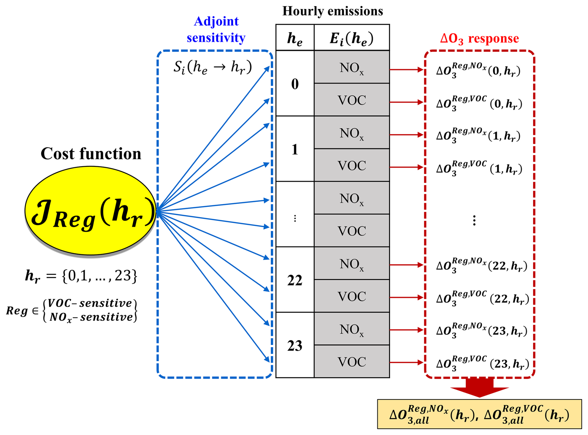
Figure 4 Schematic of the adjoint-based O₃ response calculation. A single adjoint run provides, for a given receptor hour h_r, the sensitivities of the regime-mean surface O₃ diagnostic cost function J_Reg(h_r) to precursor emissions at each emission hour h_e. Multiplying these sensitivities by the corresponding hourly emissions E_i(h_e) ($i\in \mathit{\{}{\mathrm{NO}}_x,\mathrm{VOC}\mathit{\}}$) yields the emission-time–specific O₃ response $\mathrm{\Delta }{\mathrm{O}}_{\mathrm{3}}^{\mathrm{Reg},i}\left(h_{\mathrm{e}},h_r\right)$. Summing over all emission hours h_e = 0–23 gives the emission-time–integrated response $\mathrm{\Delta }{\mathrm{O}}_{\mathrm{3},\mathrm{all}}^{\mathrm{Reg},i}\left(h_r\right)$. Responses are evaluated over grids classified as regime Reg at hour h_r, enabling regime-by-regime comparison of NO_x and VOC influences.

3 Results

3.1 Spatiotemporal corrections in NO_x and VOC emissions

To investigate the spatiotemporal changes in emissions constrained by the hybrid inverse modeling, we compared the results from the Hybrid_NOx experiment, which constrained only NO_x emissions, and the Hybrid_NOx+VOC experiment, which simultaneously constrained both NO_x and VOC emissions, with those based on the Prior emissions. Prior to the hybrid inversion, an L-curve test was conducted to determine an appropriate γ for the 4D-Var inverse modeling and a value of γ=10 was selected (Fig. S3).

Figure 5 shows the spatial distributions of NO_x, AVOC, and BVOC emissions averaged over the study period for the Prior and Hybrid_NOx+VOC experiments. In the Hybrid_NOx experiment, NO_x emissions were substantially reduced relative to the Prior experiment, particularly over major urban regions such as the Seoul Metropolitan Area (SMA), Busan, Ulsan, and Daegu (Fig. S4). On average, NO_x emissions across the entire modeling domain decreased by 18.23 %. The Hybrid_NOx+VOC experiment also showed a reduction in NO_x emissions, but to a lesser extent, with an average decrease of 15.5 %. In contrast, VOC emissions remained unchanged in the Hybrid_NOx experiment. However, in the Hybrid_NOx+VOC experiment, emissions of both AVOC and BVOC were substantially increased by approximately 70.54 % and 161.64 %, respectively, relative to the Prior. The increase in AVOC was largely concentrated over urban regions, similar to the NO_x distribution, while BVOC showed a more spatially homogeneous enhancement, especially over vegetated and mountainous areas across South Korea.

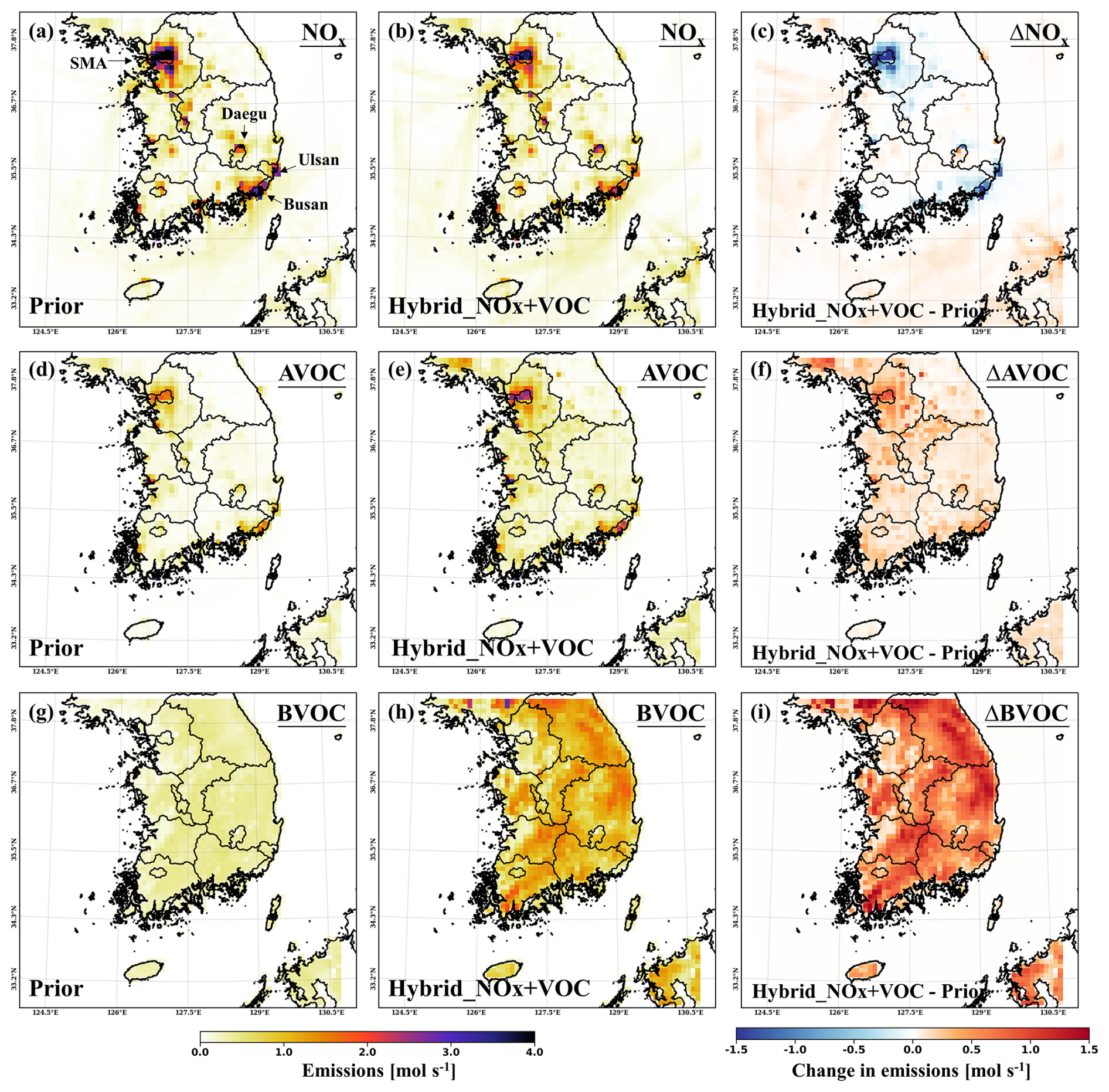
Figure 5 Spatial distributions of (a, d, g) the Prior emissions, (b, e, h) the Hybrid_NOx+VOC emissions, and (c, f, i) the corresponding analysis increments (Hybrid_NOx+VOC – Prior) for NO_x, AVOC, and BVOC, respectively, averaged over the study period.

The different adjustment magnitudes for AVOC and BVOC emissions in the Hybrid_NOx+VOC experiment arise from the distinct VOC species compositions of the two source categories and the associated differences in their chemical reactivity. Because the HCHO-based optimization updates emissions according to precursor-specific sensitivities, AVOC and BVOC emissions can be adjusted by different amounts. A similar tendency was reported in Choi et al. (2022), where BVOC emissions showed larger adjustments than AVOC when constrained with HCHO column observations. These results indicate that the VOC adjustments in our inversion reflect the species-dependent sensitivities inherent in HCHO-based optimization. Nevertheless, the large BVOC adjustment should be interpreted with caution. Because HCHO columns indirectly constrain VOC emissions, the inversion may partly compensate for uncertainties in model chemistry, oxidative capacity, transport, or retrieval errors rather than reflecting BVOC emission errors alone (Choi et al., 2025). To evaluate the consistency of the optimized BVOC emissions, we compared the modeled isoprene VCDs against the multi-year May mean CrIS retrievals for 2012–2020 (Wells and Millet, 2022). Although the Hybrid_NOx+VOC experiment produced isoprene VCD magnitudes closer to the CrIS retrievals than the Prior experiment (MBE decreased from $-\mathrm{7.16}\times {\mathrm{10}}^{\mathrm{14}}$ molec. cm⁻² in the Prior experiment to $-\mathrm{3.73}\times {\mathrm{10}}^{\mathrm{14}}$ molec. cm⁻² in the Hybrid_NOx+VOC experiment), spatial differences remained (Fig. S5). These discrepancies are likely related, at least in part, to the temporal mismatch between the multi-year May mean CrIS observations and our specific May 2022 episodic simulation. Therefore, the optimized BVOC emissions in this study should be viewed as HCHO-constrained effective VOC corrections within the model framework, rather than as an independent evaluation of absolute BVOC emission magnitudes.

Figure 6 presents the diurnal variations in NO_x, AVOC, and BVOC emissions for each experiment. The Prior NO_x emissions show two peaks corresponding to morning and evening rush hours. In contrast, the Hybrid_NOx and Hybrid_NOx+VOC experiments exhibit a shift in temporal emission patterns, with increased emissions in the morning and substantial reductions in the evening and at night. This shift implies a redistribution of hourly emission characteristics driven by the inversion process. For VOC, the Hybrid_NOx+VOC experiment resulted in a substantial increase in AVOC emissions during the daytime and a slight increase at night. BVOC emissions, which are primarily driven by photosynthetic and metabolic processes in vegetation, also showed a distinct increase during the daytime, reflecting a temporal pattern similar to that of the Prior emissions.

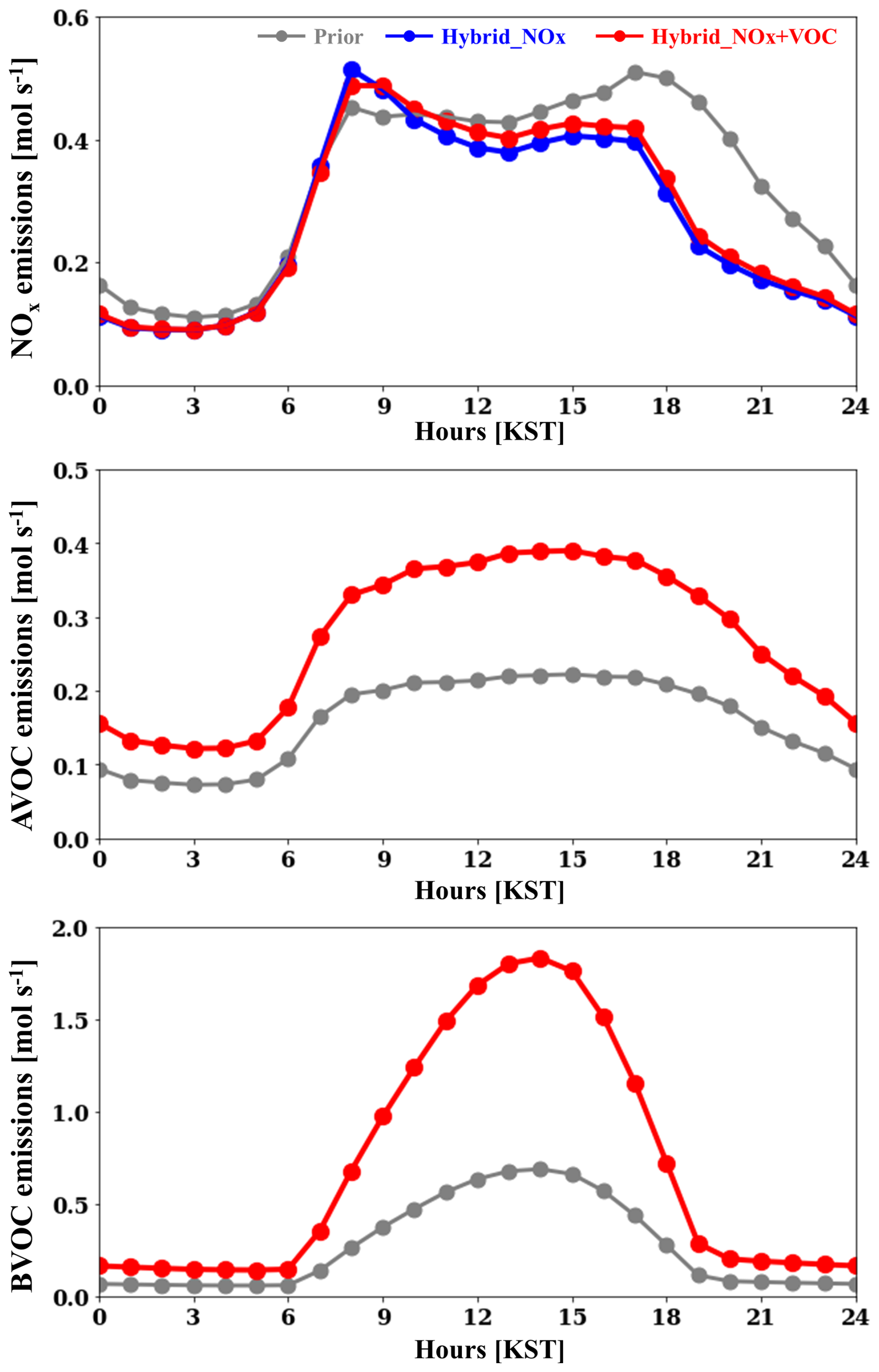
Figure 6 Diurnal variations of NO_x (top), AVOC (middle), and BVOC (bottom) emissions for each experiment (Prior: gray, Hybrid_NOx: blue, Hybrid_NOx+VOC: red), averaged over South Korea during the study period. In the Hybrid_NOx experiment, AVOC and BVOC emissions are identical to those in the Prior experiment. The Prior emissions are derived from the EDGAR-HTAPv3 inventory for anthropogenic sources and from MEGAN v2.1 for BVOC emissions.

In summary, the Hybrid_NOx+VOC experiment led to an overall reduction in NO_x emissions and an increase in VOC emissions relative to the Prior inventory. Although NO_x emissions decreased on average, they increased during the morning rush hour and decreased markedly during the evening and nighttime, indicating a shift in their temporal distribution. These results demonstrate that the proposed hybrid inverse modeling framework effectively adjusts both the spatial distribution and temporal allocation of emissions.

3.2 Spatiotemporal corrections in NO₂, HCHO, and O₃ concentrations

In this section, CMAQ simulations based on the Prior, Hybrid_NOx, and Hybrid_NOx+VOC experiments were performed to assess the effectiveness of the hybrid inverse modeling approach. Before evaluating the inverse modeling performance, the meteorological fields were first validated, with the results summarized in Table S5. The model showed good agreement with observations for temperature, wind speed, and relative humidity. Subsequently, the simulated NO₂, O₃, and HCHO concentrations for each experiment were evaluated against observational data, as summarized in Table 1.

Table 1 Statistical evaluation of AQMS NO₂, AQMS O₃, Pandora NO₂ VCD, and Pandora HCHO VCD for each experiment (Prior, Hybrid_NOx, and Hybrid_NOx+VOC). The statistics were calculated over the corresponding observation locations and averaged over the entire study period. Surface NO₂ and O₃ observations were obtained from the AQMS network, while NO₂ and HCHO VCD observations were obtained from Pandora measurements.

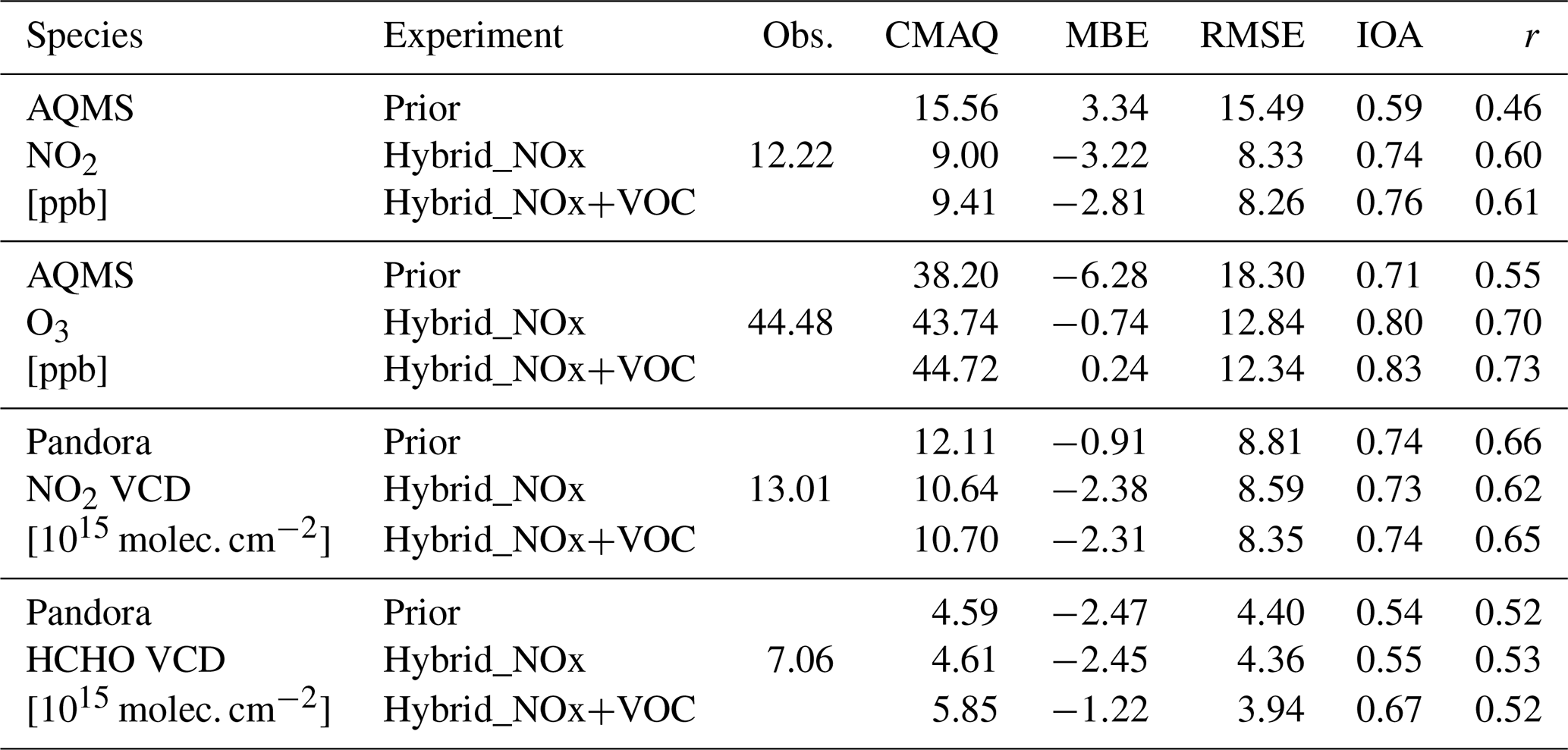
For NO₂, the Prior experiment exhibited a positive bias, with a mean bias error (MBE) of 3.34 ppb. This overestimation was notably reduced in the Hybrid_NOx and Hybrid_NOx+VOC experiments, with MBEs of −3.22 and −2.81 ppb, respectively. The temporal pattern of bias also changed: while the Prior experiment overestimated NO₂ concentrations during nighttime, both hybrid simulations substantially reduced this overprediction, resulting in concentrations closer to observations (Fig. 7). These improvements, primarily attributable to decreased nighttime NO_x emissions, led to enhanced agreement during nighttime. Consequently, the correlation coefficient (r) increased from 0.46 in the Prior experiment to above 0.6 in both hybrid experiments. As an additional column-based evaluation, the simulations were compared with Pandora NO₂ VCD observations. The Hybrid_NOx+VOC experiment slightly reduced the root mean square error (RMSE) relative to the Prior experiment, but the MBE became more negative, with only marginal changes in the index of agreement (IOA) and correlation coefficient. This limited response is consistent with the comparison against daytime AQMS NO₂ concentrations (Fig. 7), which showed only minor changes after the inverse modeling because 4D-Var inversion mainly adjusted NO_x emissions to correct nighttime NO₂ overestimation rather than daytime NO₂ levels.

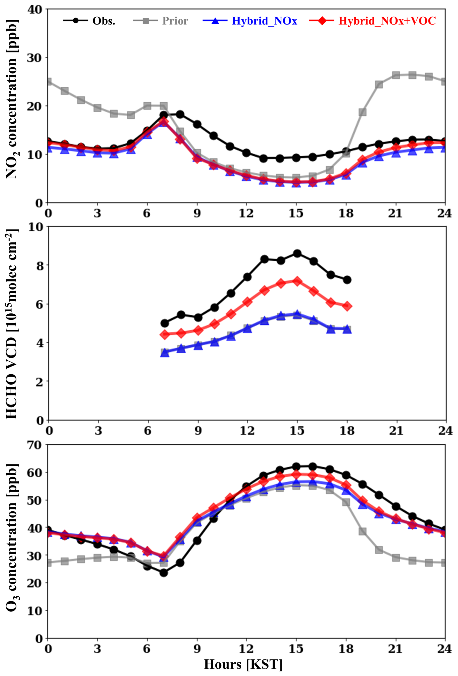
Figure 7 Diurnal variations of NO₂ concentrations (top), HCHO VCDs (middle), and O₃ concentrations (bottom) for each experiment (Prior: gray, Hybrid_NOx: blue, Hybrid_NOx+VOC: red, Observations: black) in comparison to the observations. NO₂ and O₃ are averaged over AQMS sites in South Korea, whereas HCHO VCDs are averaged over the five Pandora sites during the study period.

For VOC, model results were compared with Pandora HCHO VCDs (Table 1). The Prior experiment showed a significant underestimation (MBE = $-\mathrm{2.47}\times {\mathrm{10}}^{\mathrm{15}}$ molec. cm⁻²). The Hybrid_NOx experiment showed marginal changes in HCHO VCDs (MBE = $-\mathrm{2.45}\times {\mathrm{10}}^{\mathrm{15}}$ molec. cm⁻²) because VOC emissions were held constant; the slight difference from the Prior is attributable to secondary changes in atmospheric oxidative capacity driven by the NO_x emission updates. In contrast, the Hybrid_NOx+VOC experiment more effectively reduced the bias (MBE = $-\mathrm{1.22}\times {\mathrm{10}}^{\mathrm{15}}$ molec. cm⁻²) and achieved the highest IOA (0.67), a standardized measure of agreement between model simulations and observations, with a value of 1 indicating perfect agreement. During daytime, HCHO VCDs in both the Prior and Hybrid_NOx experiments were underestimated relative to Pandora observations, whereas the Hybrid_NOx+VOC experiment yielded higher HCHO VCDs that were closer to the Pandora measurements (Fig. 7). These results demonstrate that the underestimation of VOC emissions in the Prior experiment was effectively corrected in the Hybrid_NOx+VOC experiment, leading to improved agreement with observations across South Korea.

Regarding O₃, the Prior experiment underestimated surface concentrations, with an MBE of −6.28 ppb. The bias was substantially reduced in the Hybrid_NOx (MBE = −0.74 ppb) and Hybrid_NOx+VOC (MBE = 0.24 ppb) experiments. The IOA improved from 0.71 (Prior) to 0.80 (Hybrid_NOx) and 0.83 (Hybrid_NOx+VOC), indicating improved consistency with the AQMS observations used in the baseline inversion. In terms of diurnal variation, the Prior experiment generally underestimated O₃ with particularly large negative biases at night. In the Hybrid_NOx experiment, nighttime O₃ concentrations increased markedly, although daytime changes were limited. By contrast, the Hybrid_NOx+VOC experiment increased O₃ concentrations during both daytime and nighttime, yielding the closest agreement with observations. Spatially, the Prior experiment substantially underestimated O₃ concentrations in urban areas with high NO_x emissions, whereas the Hybrid_NOx+VOC experiment produced higher O₃ levels in these regions, resulting in improved agreement with the observations (Fig. 8).

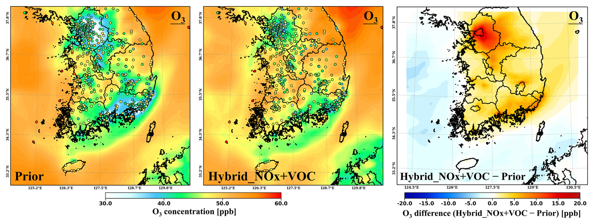
Figure 8 Spatial distributions of mean surface O₃ concentrations from the Prior (left) and Hybrid_NOx+VOC (middle) experiments, and the differences (Hybrid_NOx+VOC − Prior; right), averaged over the study period. Circles indicate O₃ observations from the AQMS network.

These improvements can be explained by the reduced titration of O₃ by NO during nighttime, which increased nighttime O₃ concentrations and improved agreement with observations. The limited daytime response in the Hybrid_NOx experiment further indicates that constraining NO_x emissions alone is insufficient to fully reproduce daytime O₃ variability. In contrast, the Hybrid_NOx+VOC experiment improved O₃ simulations during both daytime and nighttime. These findings demonstrate that jointly constraining NO_x and VOC emissions is more effective than constraining NO_x alone in accurately reproducing O₃ concentrations over South Korea.

As described in Sect. 2.2.1, the independent validation experiment produced similar improvements at the withheld AQMS sites, indicating that the posterior emission corrections were not solely a result of fitting the assimilated observations. Compared with the Prior experiment, the Hybrid_NOx+VOC experiment reduced the RMSEs for both NO₂ and O₃ and improved their temporal agreement with independent AQMS observations (Table S6). These results support the robustness of the posterior emissions and indicate that the hybrid inversion framework improves O₃ simulations beyond the stations directly used in the inversion.

3.3 Improvement of O₃ sensitivity regimes through hybrid inversion

In this section, we examine how the O₃ sensitivity regime changes before and after the application of the hybrid inverse modeling. The O₃ sensitivity is diagnosed using the HCHO-to-NO₂ ratios. Figure 9 compares the HCHO-to-NO₂ ratio distributions derived from TROPOMI with those simulated in the Hybrid_NOx+VOC experiment (see Fig. S6 for the comparison with the Prior experiment). The TROPOMI-based HCHO-to-NO₂ ratios indicate VOC-sensitive regimes over major urban regions such as the SMA, Busan, Ulsan, and Daegu, whereas NO_x-sensitive regimes dominate over mountainous and heavily vegetated areas where BVOC emissions are substantial.

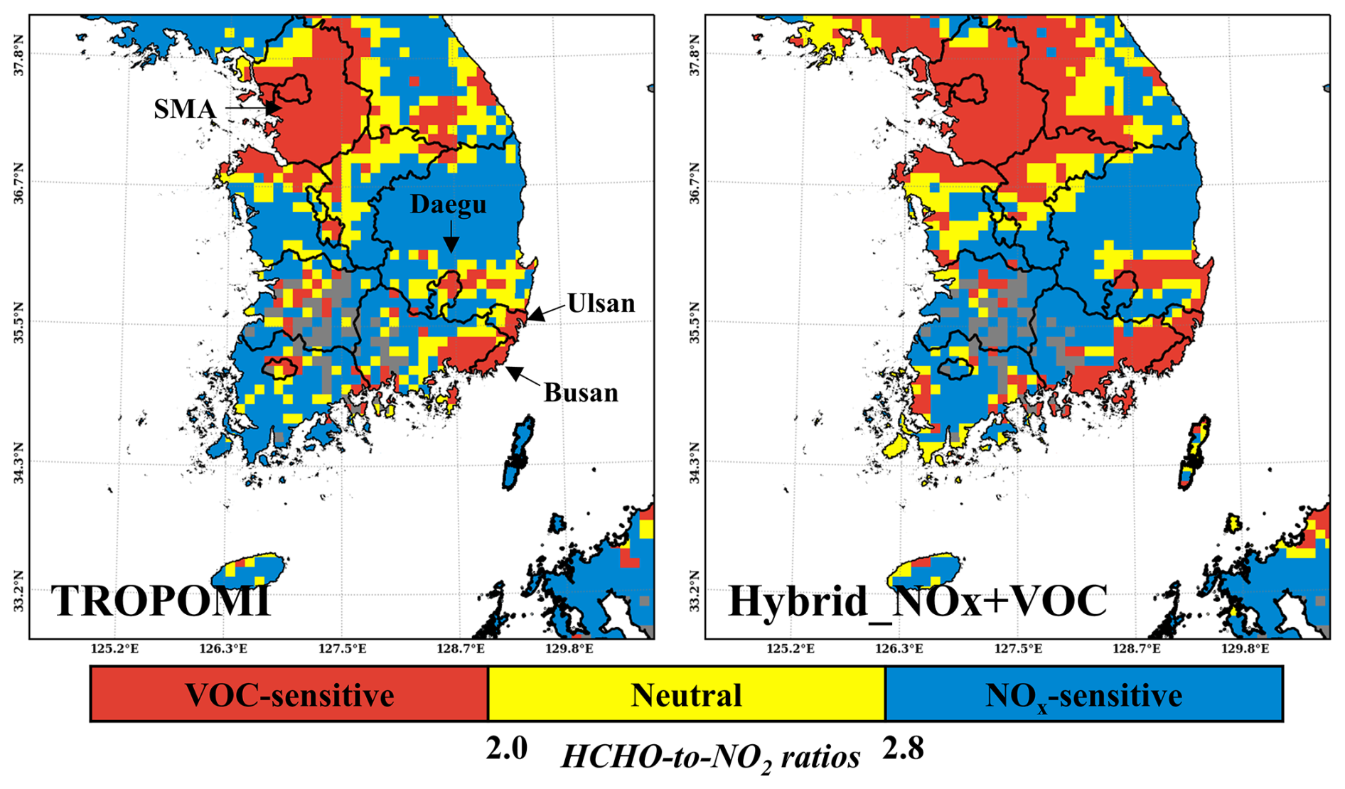
Figure 9 Spatial distributions of O₃ sensitivity regimes derived from TROPOMI-based HCHO-to-NO₂ ratios (left), and Hybrid_NOx+VOC experiment (right), averaged over the study period. Red, yellow, and blue denote VOC-sensitive, neutral, and NO_x-sensitive regimes. Gray areas denote missing or filtered pixels (e.g., due to cloud interference); for consistency, model results are sampled only at locations and times with valid satellite observations. Oceanic regions are masked to focus on terrestrial emission impacts.

The Hybrid_NOx+VOC experiment successfully reproduces the spatial pattern of the TROPOMI-based HCHO-to-NO₂ ratios, in sharp contrast to the Prior and Hybrid_NOx experiments, which classify most of South Korea as VOC-sensitive (Fig. S6). This discrepancy in the Prior experiment may partly reflect uncertainties in the prior emission inputs. The prior anthropogenic emissions are based on the 2018 EDGAR-HTAPv3 inventory, whose earlier base year may not fully represent anthropogenic emission conditions in 2022, potentially biasing the Prior experiment toward VOC-sensitive regimes. In addition, BVOC emissions estimated using MEGAN v2.1 may contribute to regime-classification uncertainty, particularly over vegetated and mountainous regions where BVOCs strongly affect HCHO production and thus the HCHO-to-NO₂ ratios. The limited improvement in the Hybrid_NOx experiment further indicates that adjusting NO_x emissions alone is insufficient to capture the observed O₃ sensitivity regimes. These results suggest that simultaneous optimization of both NO_x and VOC emissions is essential for accurately diagnosing O₃ chemical regimes.

The improved agreement in the Hybrid_NOx+VOC experiment highlights the importance of integrating recent satellite observations into emission updates, enabling the model to better reflect the current photochemical environment. These findings are consistent with recent studies reporting regional transitions in East Asia from VOC-sensitive toward NO_x-sensitive or transitional regimes (Lee et al., 2021; Itahashi et al., 2022; Wang et al., 2025).

Given that the hybrid inversion yields O₃ sensitivity regimes that closely resemble those derived from TROPOMI, the optimized posterior state provides a robust foundation for further analysis. Accordingly, in Sect. 3.4, we assess the regime-dependent hourly ΔO₃ responses to NO_x and VOC emissions using adjoint sensitivities derived from the posterior simulation.

3.4 Regime-dependent hourly ΔO₃ responses to NO_x and VOC emissions

We quantify hourly ΔO₃ responses using adjoint sensitivities to determine, within VOC-sensitive and NO_x-sensitive regimes, which precursor (NO_x or VOC) exerts a stronger influence on O₃ production or loss. Figure 10 shows regime-stratified hourly ΔO₃ responses to NO_x and VOC emissions, averaged by hour of the day over the period of 1–14 May 2022. Figure 10a and c show the ΔO₃ at each local hour (Korean Standard Time, KST), representing the cumulative response to precursor emissions released across all prior times (Eq. 12). This reflects not only the response to emissions released at the same hour but also the influence of the full diurnal emission profile of each precursor on hourly O₃. Thus, the panels illustrate how the complete daily emission cycle of each precursor contributes to hourly O₃ within each regime.

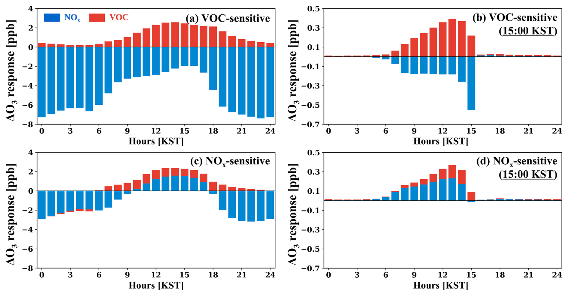
Figure 10 Two-week mean ΔO₃ response (ppb) to NO_x (blue) and VOC (red) emissions, by local hour, for 1–14 May 2022. For each local hour, responses are spatially averaged over grid cells classified into each regime at that hour; regimes are diagnosed with the HCHO-to-NO₂ ratios from the Hybrid_NOx+VOC experiment. Panels (a) and (c) show, for VOC-sensitive and NO_x-sensitive regimes respectively, the ΔO₃ response at each local hour to emissions released over all hours (i.e., emission-time–integrated response). Panels (b) and (d) show the ΔO₃ response at 15:00 KST as a function of emission time (“emission-time response”).

In the VOC-sensitive regime (NO_x-rich), the NO_x response is negative at all hours, indicating net O₃ decreases consistent with rapid O₃ titration, whereas the VOC response is positive and strengthens during daytime, reflecting enhanced photochemical production. In the NO_x-sensitive regime (VOC-rich), VOC provides a persistent positive daytime response, while the NO_x response changes sign with time of day: negative at night (titration) and positive from late morning into the afternoon as radical chemistry intensifies. A slight negative VOC response also appears during nighttime under NO_x-sensitive conditions. To clarify this response, we further separated the VOC sensitivity into AVOC and BVOC contributions (Fig. S7). The results indicate that this nighttime O₃ decrease is mainly associated with the BVOC category. This response can be explained by direct ozonolysis of reactive unsaturated VOC species represented within the BVOC category. Under nighttime conditions, when NO₂ photolysis and photochemical O₃ production are suppressed, reactions between O₃ and reactive VOC species can act as a net gas-phase O₃ sink, leading to O₃ depletion. Previous laboratory and field studies provide a chemical basis for this interpretation, showing that reactive BVOCs can undergo ozonolysis and that gas-phase reactions involving biogenic hydrocarbons can contribute to O₃ loss in forest environments (Atkinson and Arey, 2003; Kurpius and Goldstein, 2003).

Figure 10b and d focus on 15:00 KST, the hour of maximum O₃ concentration, to illustrate the sensitivity of O₃ at this hour to the timing of precursor emissions. This allows for a comparison of how hourly emissions contribute to the O₃ concentration at 15:00 KST (Eq. 11). In VOC-sensitive regimes, NO_x emitted at 15:00 KST yields the largest negative ΔO₃ response, consistent with the instantaneous O₃ titration. By contrast, VOC emissions at 13:00 KST exert the strongest positive influence on 15:00 KST O₃, indicating an effective lag of about 2 h associated with multistep photochemical production. In NO_x-sensitive regimes, NO_x generally promotes O₃ formation; however, NO_x emitted at 15:00 KST still produces O₃ losses through immediate titration. The largest positive effects on 15:00 KST O₃ arise from NO_x at 13:00 KST and VOC at 14:00 KST, indicating a similar response time of approximately 1–2 h.

Taken together, the results show that precursor impacts on O₃ vary with both regime and hour. Under VOC-sensitive conditions, VOC reductions are more effective than NO_x reductions for lowering daytime O₃, whereas under NO_x-sensitive conditions, NO_x controls deliver the more direct decreases. Because titration is immediate but photochemical production requires chemical processing time, effective mitigation of high-O₃ periods requires hour-specific emission controls aligned with the prevailing O₃ sensitivity regime. These results also indicate that emission control strategies should not be based solely on daily mean precursor responses. In VOC-sensitive regions, nighttime NO_x emissions decrease O₃ through NO titration; therefore, stricter nighttime NO_x controls may not immediately reduce O₃ and could increase nighttime O₃ by weakening titration. In contrast, VOC reductions are more effective for lowering daytime O₃ under VOC-sensitive conditions, whereas NO_x reductions provide a more direct pathway for reducing daytime O₃ under NO_x-sensitive conditions.

Furthermore, to assess the practical efficiency of VOC emission controls, it is crucial to distinguish between anthropogenic and biogenic sources, as only AVOCs can be actively regulated. As shown in the separated VOC contributions (Fig. S7), the contribution of AVOCs to O₃ formation is small in the NO_x-sensitive regime. In the VOC-sensitive regime, however, AVOCs account for approximately 14 % to 21 % of the total VOC-driven O₃ response, indicating a non-negligible potential for targeted AVOC controls in these specific areas. Nevertheless, BVOCs still predominantly drive the overall O₃ responses across the domain. We attribute this strong BVOC dominance to the specific study period (May), which is characterized by highly active biogenic emissions. Therefore, the influence of BVOCs observed in this study might be more pronounced than in other seasons, such as autumn or winter, when biogenic activities significantly decrease. Consequently, the potential effectiveness of AVOC controls can vary considerably by season, and our findings regarding the limited impact of AVOC reductions should be interpreted with the seasonal characteristics of the study period in mind.

A clear understanding of how precursor influences on O₃ differ across sensitivity regimes and vary throughout the day is essential for designing realistic and region-specific O₃ control strategies. In this context, the hybrid inversion framework presented in this study provides a practical basis for policy development, as it enables accurate identification of the dominant O₃ sensitivity regime and quantification of the major precursor contributions. By capturing both the chemical regime and the temporal characteristics of precursor impacts, the proposed methodology can provide valuable guidance for developing region-specific and effective emission reduction strategies. The comparison between the Prior and posterior (Hybrid_NOx+VOC) simulations further demonstrates the value of using observation-constrained emissions to refine policy-relevant O₃ sensitivity diagnostics. As shown in Fig. S6, the Prior experiment classified most of South Korea as VOC-sensitive, suggesting that VOC reductions would be broadly prioritized based on the Prior emissions. In contrast, the posterior results identified substantially more NO_x-sensitive regions, where NO_x reductions are expected to be more effective than VOC reductions for lowering daytime O₃. Thus, the posterior simulation complements the Prior inventory by providing a more spatially differentiated diagnosis of target precursors for emission control. Moreover, because the posterior NO_x emissions showed a substantial nighttime reduction relative to the Prior emissions (Fig. 6), the inferred timing of effective controls could also differ between the Prior and posterior simulations. These differences demonstrate that posterior, observation-constrained emissions provide a more reliable basis for deriving spatially targeted, time-specific, and chemically appropriate O₃ mitigation strategies.

This analysis is limited to a two-week period and may not capture the seasonal or longer-term variability of O₃ sensitivity regimes across South Korea. Nevertheless, the hybrid inverse modeling framework efficiently constrains precursor emissions on short time scales and enables assessments tailored to individual regions that explicitly account for the prevailing O₃ sensitivity regime, thereby supporting the implementation of emission reduction policies. Compared with conventional bottom-up inventories, the top-down approach uses atmospheric observations to adjust prior emissions and provide posterior emission estimates that are more consistent with observed concentrations. A full-year hybrid inversion would require FDMB and repeated 4D-Var assimilation cycles and therefore substantial computational resources. However, compared with developing or updating bottom-up inventories based on detailed activity data and source-specific emission factors, the top-down approach can provide relatively rapid observation-driven emission estimates. This approach enables rapid updates of O₃ precursor emissions and provides timely guidance for O₃ management policies.

4 Summary and Conclusions

This study aimed to enhance the accuracy of simulated O₃ concentrations and improve the diagnosis of O₃ sensitivity regimes over South Korea by applying a top-down hybrid inverse modeling approach to constrain the spatiotemporal distributions of NO_x and VOC emissions, and to quantify hourly ΔO₃ responses to these precursors using adjoint sensitivities. The inverse modeling system used TROPOMI NO₂ and HCHO column densities along with surface NO₂ and O₃ measurements from the AQMS network. The modeling was conducted using CMAQ and its adjoint model. The hybrid inverse modeling approach combining the FDMB and 4D-Var methods was employed to constrain emissions. To assess the impact of major O₃ precursors on the spatiotemporal distribution and sensitivity regime of O₃, three experiments were conducted: Prior, which used EDGAR-HTAPv3 for anthropogenic emissions and MEGAN v2.1 for biogenic VOC emissions; Hybrid_NOx, in which only NO_x emissions were optimized; and Hybrid_NOx+VOC, in which both NO_x and VOC emissions were jointly constrained.

In the Hybrid_NOx experiment, where only NO_x emissions were adjusted, emissions decreased by up to 51 % at night and increased by up to 14 % during the day relative to the Prior inventory, resulting in an overall average reduction of 18 %. These time-dependent adjustments enabled the correction of diurnal variability in the emission profile. In the baseline comparison with AQMS observations used in the inversion, nighttime O₃ concentrations increased and the negative O₃ bias was substantially reduced relative to the Prior experiment. In contrast, during the daytime, constraining NO_x emissions alone yielded only limited improvements in O₃ concentrations. This highlights the need for jointly constraining NO_x and VOC emissions to better represent the nonlinear chemical processes controlling daytime O₃ formation.

To address this limitation, the Hybrid_NOx+VOC experiment was conducted, in which both NO_x and VOC emissions were simultaneously constrained. Compared to the Prior emissions, NO_x emissions decreased by an average of 15.5 %, while AVOC emissions and BVOC emissions increased by 71 % and 162 %, respectively. In the independent data-splitting validation, in which 20 % of AQMS sites were withheld from the inversion, the Hybrid_NOx+VOC experiment reduced the magnitude of O₃ MBE from 3.02 to 0.86 ppb and increased IOA from 0.71 to 0.77 relative to the Prior experiment. These independent validation results support the robustness of the posterior emission corrections and underscore the importance of simultaneously constraining NO_x and VOC emissions and accurately representing their diurnal variability for improving O₃ model performance.

The hybrid inverse modeling also improved the simulation of O₃ sensitivity regimes. In the Hybrid_NOx+VOC experiment, the spatial distribution of the simulated HCHO-to-NO₂ ratios closely matched the TROPOMI-derived regimes, reproducing VOC-sensitive conditions over major urban regions and NO_x-sensitive conditions over mountainous and vegetated areas. This agreement highlights the ability of the hybrid inversion to incorporate observational constraints and accurately represent the relative contributions of NO_x and VOC to O₃ formation. The improved regime classification further provides a reliable foundation for analyzing regime-dependent O₃ production and understanding how changes in precursor abundances drive transitions between VOC-sensitive and NO_x-sensitive conditions.

Building on the improved regime representation obtained from the Hybrid_NOx+VOC experiment, we further analyzed how each precursor influences O₃ in a regime- and time-dependent manner. Under VOC-sensitive conditions, VOC emissions sustain daytime O₃ production, whereas NO_x emissions lead to net O₃ losses through rapid titration. In contrast, under NO_x-sensitive conditions, NO_x emissions contribute positively to O₃ formation from late morning into the afternoon, while titration processes dominate during nighttime hours. These results clarify precursor-specific emission control priorities with explicit diurnal dependence: in VOC-sensitive regimes, reducing VOC emissions is most effective for mitigating daytime O₃, whereas in NO_x-sensitive regimes, NO_x emission reductions provide more immediate and direct benefits. Because titration occurs almost instantaneously while photochemical production unfolds over finite chemical timescales, effective mitigation of high-O₃ periods requires hour-specific emission controls that are aligned with the prevailing O₃ sensitivity regime. The contrast between the Prior and Hybrid_NOx+VOC experiments further highlights the value of observation-constrained posterior emissions in refining policy-relevant O₃ sensitivity diagnostics. The Prior experiment provided a broad initial indication of VOC-sensitive conditions over South Korea, while the posterior emissions revealed more spatially differentiated sensitivity regimes, including more extensive NO_x-sensitive regions. This suggests that the hybrid inversion can complement prior emission inventories by improving the representation of both the target precursor and the timing of effective emission controls. Therefore, observation-constrained posterior emissions provide an important basis for developing spatially targeted, time-specific, and chemically appropriate O₃ mitigation strategies.

This analysis spans two weeks and therefore may not capture seasonal or long-term variability. In addition, because EDGAR-HTAPv3 was spatiotemporally downscaled for CMAQ, inventory-related uncertainties could not be fully assessed. Despite these limitations, the findings suggest that extending the hybrid inverse modeling over longer periods and incorporating diverse observations would further improve the resolution and reliability of emission estimates. Overall, the proposed hybrid inverse modeling shows strong potential to enhance O₃ simulations and to support region-specific regime assessments and precursor emission control strategies.