Ozone stratospheric trends from regional Bayesian composite of ground-based partial columns

Large uncertainties and variability in individual ground-based instrument records limit the detection of statistically significant ozone trends, particularly in the lower stratosphere. Available merging studies are typically performed by latitude bands on satellite-based data records. This study derives correlation-based regional composites of ground-based timeseries towards reducing trend uncertainties. We address fundamental heterogeneities resulting from grouping individually homogenized ground-based datasets to enable robust merging. Uneven temporal and vertical resolutions of five ozone measurement techniques (Ozonesondes, FTIR, Dobson Umkehr, Lidar and Microwave radiometers) are handled by integrating monthly mean ozone profiles in two sets of four independent partial columns. Spatial heterogeneity is resolved by defining coherent regions using the Copernicus Atmosphere Monitoring Service (CAMS) reanalysis. Regional timeseries are merged by the BAyeSian Integrated and Consolidated (BASIC) algorithm, adapted to consider propagated measurement uncertainties and the agreement between individual timeseries by Principal Component Analysis (PCA). Trends for the 2000–2024 period are then estimated by Multiple Linear Regression using the LOTUS model. We compare BASIC with a conventional weighted mean. While the weighted mean fails to capture variability during periods of low instrument consensus, BASIC produces more representative timeseries by robustly handling outliers. Accordingly, for the selected regions, BASIC reduces average uncertainties of the trend estimates by 9.4 % relative to the weighted-mean approach. Our results support positive trends in the upper stratosphere, predominantly negative trends in the middle stratosphere and non-significant trends in the lower stratosphere. This study establishes a consolidated ground-based reference to be used for comparison with global satellite-based ozone trends.

1 Introduction

The Montreal Protocol and its subsequent Amendments have successfully reduced the atmospheric concentrations of ozone depleting substances, initiating a slow recovery of the ozone layer (WMO, 2022). However, this recovery is spatially heterogeneous and remains vulnerable to emerging threats such as unregulated emissions (Rigby et al., 2019) and climate change (Wang et al., 2025), emphasizing the need for continuous monitoring of both stratospheric and tropospheric ozone.

The clear recovery signal in the upper stratosphere (WMO 2022) contrasts with the evolution of ozone in the lower stratosphere, which remains uncertain (Dietmüller, 2021; Szela̧g et al., 2020; Millán et al., 2025). Statistically non-significant negative ozone trends have been estimated from measurements in the lower stratosphere while models are showing the opposite (Godin-Beekmann et al., 2022; WMO, 2022). Moreover, the large uncertainties of the trend estimates in the lower stratosphere, possibly coming from the rising tropopause in the tropics (Thompson et al., 2025), prevent definitive conclusions about ozone changes in this vertical domain. We note also that trends from individual ground-based instruments can be significantly different, even if the instruments are collocated (Petropavlovskikh et al., 2019; Godin-Beekmann et al., 2022; Björklund et al., 2024) and that large discrepancies are also reported in trend estimates from satellite-based data records (Sofieva et al., 2026). Differences in collocated data records should be taken into account when combining them using an appropriate merging technique. Nevertheless, profile trend estimation is crucial to understand the recovery processes. Ozone changes are dominated by different chemical and dynamical processes depending on the altitude (WMO, 2022). Hence, the monitoring of the vertical structure of the changes is an essential addition to that of the integral measurement, i.e. the total ozone column.

Several considerations aimed at reducing the uncertainties in ozone profile trends can be found in the literature. The merging of data records has been extensively used in the field of satellite-based instruments, with the merging of gridded satellite-based data records (Sofieva et al., 2021), the merging of homogenized satellite-based data records (Davis et al., 2016; Arosio et al., 2019) or the merging of debiased ozone records in Froidevaux et al. (2015). In the OCTAV-UTLS APARC activity, Millán et al. (2025) report the ozone profile in several coordinate systems to divide the measurements into vertical domains. This allows the data in each domain to be affected by the same dynamical processes, reducing their variability. This reduction is critical for trends detection particularly in UTLS where opposite ozone changes cancel each other in standard pressure coordinates. Integration of the vertical profiles into partial columns can also be used to partially compensate for the significant uncertainties of a profile, as it averages out its vertical variability. This method is widely used in the validation of low vertical resolution instruments with higher resolution instruments (e.g. Kramarova et al., 2013; Frith et al., 2020) or data assimilation products (e.g. Inness et al., 2019; Emili et al., 2014).

Satellites provide excellent geographical coverage, although their life-time may be more limited (e.g. SBUV series of remote sensors, SAGEII-III-IV, ENVISAT). On the other hand, ground-based instruments are geographically rather sparse and unequally distributed, but their time series are continuous (Stübi et al., 2017) and the resolution of some of them in the lower stratosphere is sufficient: less than 1 km for Lidars (Leblanc et al., 2016), a few hundred meters for ozonesondes (Smit and Thompson, 2021), and insufficient for others: MWR cannot resolve the lower-stratosphere below 20 km (Maillard Barras et al., 2020). With the foreseen reduction of the number of limb-viewing satellite instruments in the coming years (Salawitch et al., 2025), the study of ozone recovery will rely more heavily on ground-based measurements to help fill the data gaps that will emerge for ozone and other essential climate variables.

There is therefore a sustained need for ground-based global coverage of ozone measurements (which can be achieved only by increasing the number of ground-based stations. A global coverage impression can be reached by grouping the data records into regions and by considering these regions as entities with similar ozone variability). Furthermore, by combining all existing information into a regional composite, the uncertainty of the resulting time series, and thus of its trend estimate, can likely be reduced (e.g. Ball et al., 2017; Arosio et al., 2019; Sofieva et al., 2021; Keppens et al., 2025). The main motivation of this study is to improve from single-station or single-instrument trend analyses, which are often affected by local data gaps and instrumental drifts. By using a Bayesian merging methodology over coherent regions, we aim to extract the underlying regional common ozone signal. This approach takes advantage of the spatial redundancy within the NDACC network to go beyond a simple spatial average, resulting in a more stable composite for long-term trend estimation.

In this study we integrate heterogeneous ground-based ozone datasets into common partial columns, and define spatially coherent regions with correlations derived from a representativeness analysis. We merge time series into a composite using a Bayesian algorithm (BASIC, Ball et al., 2017), and estimate 2000–2024 trends with the MLR model from LOTUS (Petropavlovskikh et al., 2019; Godin-Beekmann et al., 2022) defined within the LOTUS/APARC activity (Long-term Ozone Trends and Uncertainties in the Stratosphere) with consideration of the propagated monthly measurement uncertainties. We compare the Bayesian approach to conventional weighted mean, and provide regional partial-column trend estimates.

The paper is organized as follows: ground-based instrument datasets, partial column definitions and determination of uncertainties are described in Sect. 2. Section 3 is dedicated to the methodology and describes the determination of the regions with the representativeness study based on the CAMS reanalysis, the Bayesian merging method and the MLR trend estimation. Results are detailed in Sect. 4, where regional composites are computed and their 2000–2004 trends estimated for regions covering a part of the globe. Finally, conclusions are drawn in Sect. 5.

2 Data Records

The data records used in this study are mostly part of the Network for the Detection of Atmospheric Composition Change (NDACC) (NDACC, 2020). The NDACC ozone profiles records are made of five instrument types: Ozonesondes (O3S), Fourier-Transform InfraRed spectrometers (FTIR), Lidars, Microwave Radiometers (MWR) and Dobson (Umkehr) spectrophotometer. The data records used in this study are mostly part of the Network for the Detection of Atmospheric Composition Change (NDACC), except that not all the homogenized ozonesondes site data used here belong to NDACC. The NDACC-affiliated ozonesondes data records are on the way to being submitted to the NDACC Data Host Facility by the instrument PIs after having been homogenized within the Harmonization and Evaluation of Ground-based Instruments for Free-Tropospheric Ozone Measurements (HEGIFTOM) working group of the Second Tropospheric Ozone Assessment Report (TOAR II). We strictly limit our ozonesondes selection to this HEGIFTOM dataset because it uniquely provides the per-measurement uncertainties required for our error propagation to the monthly means. Furthermore, isolated sites or instruments that do not correlate sufficiently with other NDACC records (such as specific ozonesondes in Antarctica or East Asia) are naturally excluded by our regional grouping methodology. A map of all available measurement stations by instrument type is illustrated in Fig. 1, and a table describing all the instruments names, coordinates and data availability is in Supplement Sect. S1.

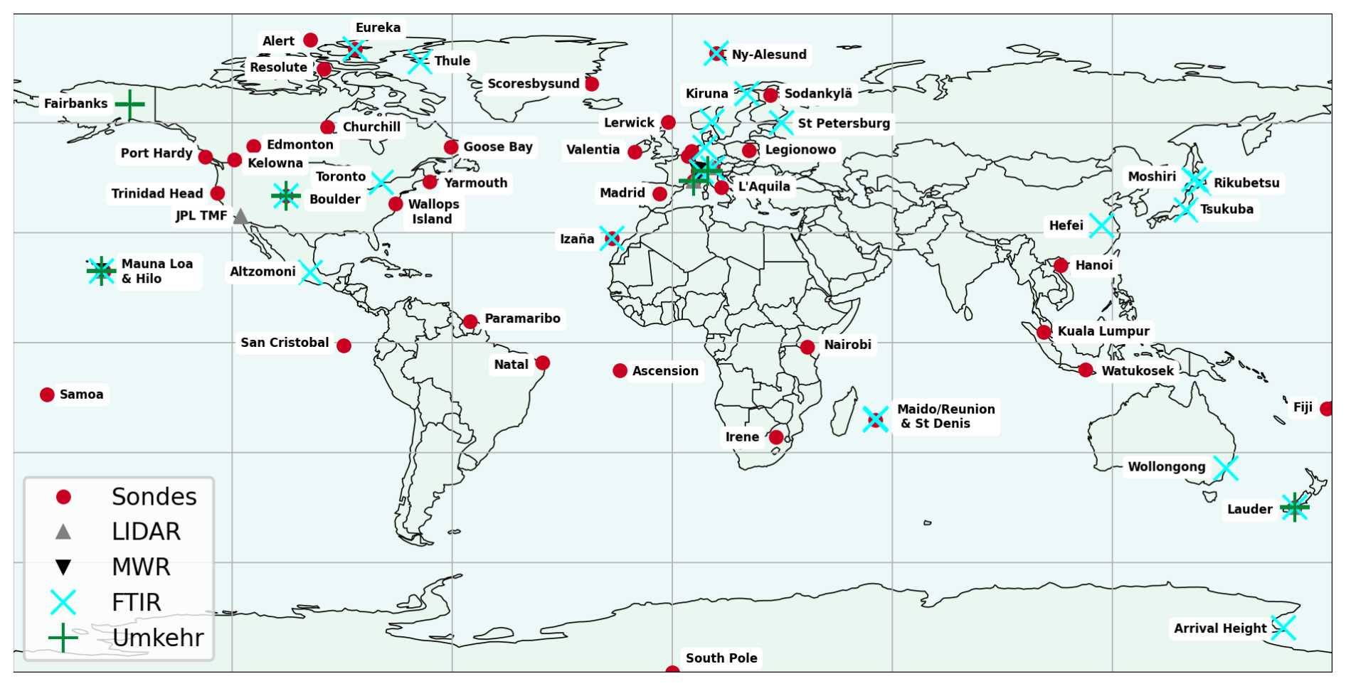
Figure 1 Map of all available measurement stations by instrument type: ozonesonde in red, LIDAR in grey, MWR in black, FTIR in cyan and Dobson Umkehr in green.

We use harmonized data records and homogenize the propagation of measurement errors. The homogenization of the time series aims to identify and correct artifacts, jumps and drifts where possible, although some inhomogeneities may remain. This harmonization work was performed within the APARC/LOTUS and TOAR-II/HEGIFTOM (Harmonization and Evaluation of ground-based Instruments for Free Tropospheric Ozone Measurements) initiatives. As a result, we assume that differences between the homogenized time series are limited to measurement (random) errors and offsets caused by variations in spatial representativeness (see Sect. 3.1).

The instruments differ significantly in their measurement principles, uncertainties and vertical resolutions. For a consistent merging of the datasets, a common basis is required, on which instruments datasets are comparable. This is achieved by integrating the profiles over defined Partial Columns (PC), which will be described in Sect. 2.1. The uneven resolutions are addressed by ensuring that at least one degree of freedom per instrument is available in each defined partial column. Figure 2 illustrates the vertical resolution of the instruments as the number of horizontal bands within their vertical ranges, alongside the two sets of partial columns defined for this study (see Sect. 2.1). The instruments also differ in temporal resolution as follows: Ozonesondes are launched typically 2 to 12 times per month, Dobson Umkehr provides bi-daily measurements at most, Lidar, FTIR and MWR can provide several profiles per hour, nighttime for the Lidar, daytime for the FTIR and both daytime and nighttime for the MWR. The diurnal cycle is not expected to contribute to the disparities caused by different temporal resolutions, given its limited amplitude, maximum in the upper stratosphere, reported to be generally below 4 % (Sauvageat et al., 2023). To reduce these disparities, we aggregate all data into monthly means (L3). This approach does not fully resolve all sampling biases: for ozonesondes, the limited launch frequency (2–12 per month) leaves monthly means potentially unrepresentative of episodic events, while for Dobson Umkehr, Lidar and FTIR, the requirement for clear-sky conditions introduces a meteorological sampling bias that monthly averaging cannot eliminate. These residual biases are partially absorbed into BASIC's posterior uncertainty through the inter-instrument disagreement, but are not explicitly corrected. Furthermore, to ensure consistency, all monthly mean partial columns are expressed in Dobson Units (DU).

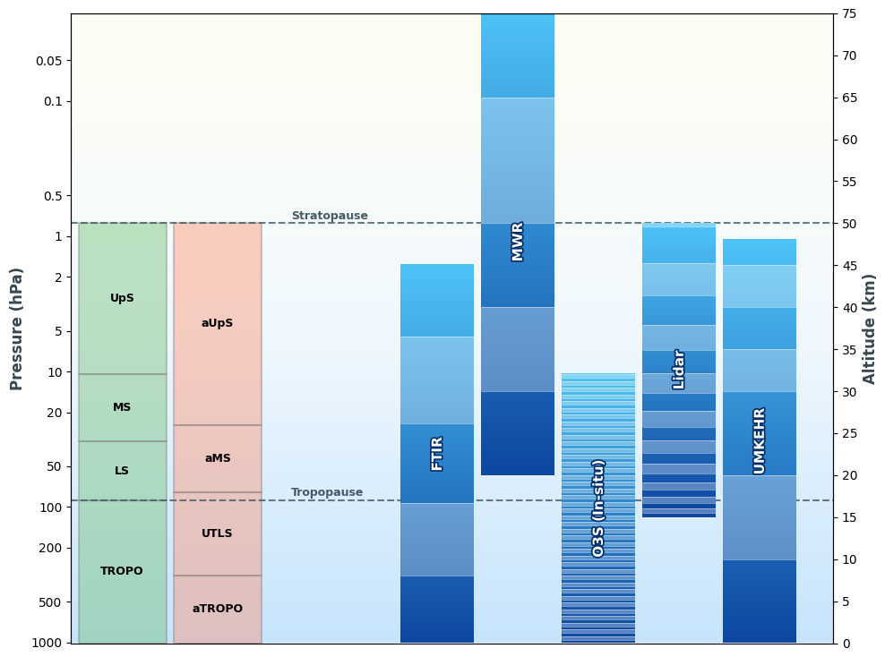
Figure 2 Representation of the two sets of partial columns used on the left-hand side and of the instruments approximate vertical resolutions and ranges on the right-hand side (adapted for ground-based ozone measurements from NDACC (link in Table S1 in the Supplement). Pressure ranges values are given in Table 1.

Finally, a consistent methodology is applied to propagate uncertainties from individual measurements (L1) to the monthly means (L3) used for trend analysis. The L1 measurement uncertainties are the total error budget, including random and systematic errors, as well as smoothing and retrieval uncertainties for remote sensing techniques. The uncertainty of the daily mean (L2) is calculated as the L1 measurement uncertainty divided by the square root of the number of measurements within that day. Then, the monthly mean uncertainty (L3) is calculated by dividing the daily L2 uncertainty by the square root of the number of measurement days in the month. Specific L1 uncertainty values are detailed in the following subsections.

2.1 Partial Columns

The proxies used in ozone trend analyses typically represent large-scale, low-frequency atmospheric variability. Small-scale or high-frequency variability is therefore not captured by the regression model, leading to larger trend uncertainties. This leads to large uncertainties in trend estimates when derived from highly resolved vertical profiles. Vertical integration may counteract this effect by averaging out some variability, if the partial columns are selected for that purpose. However, fine vertical evolution can also be averaged out by vertical integration. Focusing on reducing the uncertainties of the trends estimates, we have chosen to estimate the trends of ozone on two sets of four partial columns defined as follows (see Table 1):

• the standard set (“sPC”), which can be found in Ball et al. (2018 and 2020) with a distinction for stations with latitudes inside and outside the 30° band.

• the alternative set (“aPC”), which has a pure troposphere and a UTLS, in order to force the variability around the tropopause into a single partial column.

Table 1 sPC and aPC are two sets of partial columns defined on pressure levels (approx. heights in km) with latitude distinction. The two sets of partial columns can be seen on the left-hand side of Fig. 1. ^a Latitude < 30°, ^b Latitude < $\mathrm{15}/\mathrm{30}/\mathrm{60}/\mathrm{90}$°.

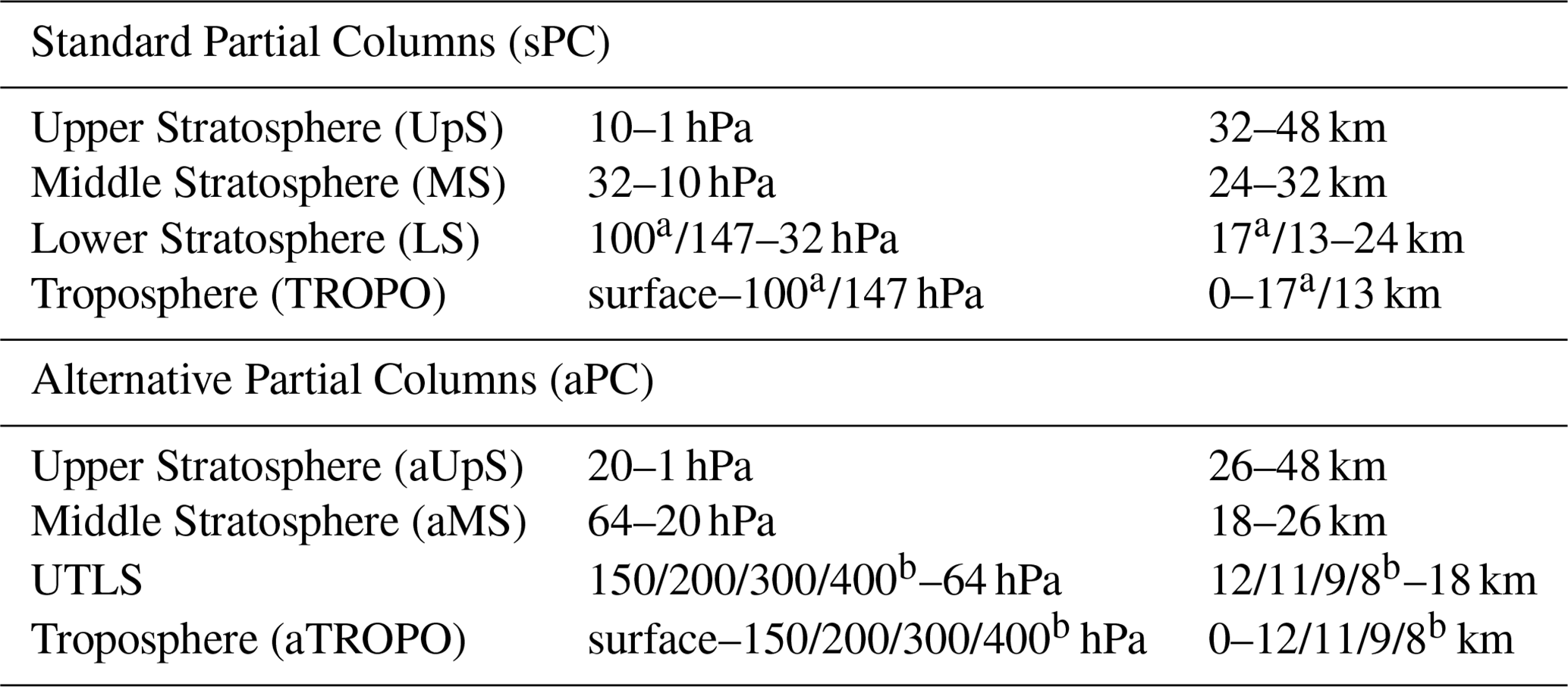
To account for the decrease in the tropopause height with increasing latitude, we define the layers depending on the latitude. For the standard partial columns, this is done using a separation at 30°, and with finer resolution for the alternative partial columns, to ensure that the boundaries remain consistent with the climatological tropopause height.

The daily tropopause variability is not included, which contributes to the noise in LS and UTLS layers. This could be addressed in future work by including a dynamical proxy for the tropopause height.

For all instrument types, the ozone amount in each partial column has been computed as the sum of ozone content in function of the pressure level within the partial columns' vertical ranges. Ozonesondes do not provide any values in the upper stratosphere, MWR do not provide any tropospheric nor UTLS ozone values and Lidars provide a complete stratosphere as described in Sect. 2.2.3. Monthly means are computed from daily mean values. The minimum number of measurement days per month was set to three.

2.2 Instruments

2.2.1 Ozonesondes

Ozonesondes, launched with weather balloons, are small, light-weight instruments that measure the vertical ozone profile up to about 30–35 km altitude (10–5 hPa), based on the titration of ozone in a neutral buffered potassium iodide sensing solution. This measurement technique has a stated precision better than ±(3 %–5 %) and an accuracy of about ±(5 %–10 %) for up to 30 km altitude (Smit et al., 2021, 2024). As major contributors to uncertainties in ozone trends are discontinuities and biases in the long-term records of ozonesonde sites due to e.g. changes in ozonesonde type, sensing solution, and preparation/processing, the ozonesonde data has been homogenized as described in Smit et al. (2021), Van Malderen et al. (2025a), and references therein. This homogenization (normally) also involves the provision of an uncertainty estimate for every single measurement. To calculate partial ozone columns from the ozonesonde data, the profiles are simply integrated between the upper and lower boundaries of the defined atmospheric layers, if the percentage of missing (intermediate) profile data in the partial column is not higher than 20 %. The uncertainties of the partial ozone columns are obtained by summing up the individual uncertainties of the ozone concentration measurements across pressure levels. Since the same instrument measures all layers during a given flight, the measurements at different altitudes are not linearly independent. This linear sum is the worst case scenario, assuming fully correlated systematic uncertainties in the entire vertical profile. Most sites typically launch once a week, but the average monthly launch frequencies vary roughly within the ozonesonde network between 2 to 12. The uncertainties on the monthly means have been computed as described above (see Sect. 2) and are around 5 % to 6 % on average. While other ozonesonde records exist globally, our analysis is restricted to the HEGIFTOM dataset, which uniquely provides the per-measurement uncertainties required for our error propagation. Furthermore, isolated sites or instruments that do not correlate sufficiently with other NDACC records (such as specific sites in Antarctica or East Asia) are naturally excluded by our regional grouping methodology.

2.2.2 FTIR

The FTIR (Fourier Transform InfraRed) ozone measurements are uniformly performed in NDACC with Bruker high-resolution spectrometers (except for Toronto, which uses an ABB Bomem instrument). This remote sensing technique retrieves trace gas concentrations from solar absorption spectra, requiring daylight and cloud-free conditions. The FTIR ozone retrievals have been standardized within the IRWG (InfraRed Working Group, https://www2.acom.ucar.edu/irwg, last access: 8 July 2026). Details on the instruments, retrieval codes and principles can be found in Vigouroux et al. (2015). In summary, ozone total columns can be retrieved from the area of ozone absorption lines by fitting spectral regions modelized using a spectroscopic database (HITRAN), climatological a priori profile information on all absorbing gases, and a radiative transfer model. Profiles of limited vertical resolution can be obtained from the line shapes (pressure and temperature dependent) by using regularization techniques. The vertical resolution and degrees of freedom for signal (DOFS) are described by the averaging kernels. For ozone, the sensitivity covers the surface up to about 48 km, with about 4 DOFS: one in the troposphere and three in the stratosphere (Vigouroux et al., 2015).

Except for Altzomoni and Izana, the present paper uses the latest improved version of NDACC FTIR ozone data (Bjorklünd et al., 2024), in which the spectral windows have been optimized to avoid water vapor line interferences while the spectroscopic parameters have been updated to HITRAN 2020 (Gordon et al., 2022)

The uncertainty characterization is based on optimal estimation (Rodgers, 2000; and Vigouroux et al., 2015 for details on its application to FTIR ozone retrievals). The random part is dominated by the measurement noise for total columns (about 1.0 %–1.4 % for an individual measurement) and by the smoothing random uncertainty for partial columns (about 4 %–6 %). The systematic uncertainty is dominated by spectroscopy, especially for total columns (2 %–3 %), and by the instrumental line shape and the temperature a priori profile errors for the partial columns (5 %–7 %).

2.2.3 Lidar

Lidar (Light Detection And Ranging) is a remote sensing technique based on the interaction of coherent light source with the atmosphere. The use of pulsed laser sources enables range-resolved measurements (active remote sensing). Ozone measurements by lidar are performed using the DIAL (Differential Absorption Lidar) technique, which uses the simultaneous emission of two laser wavelengths absorbed differently by ozone in the atmosphere. For stratospheric ozone, the weakly-absorbed wavelength of 308 nm and non-absorbed wavelength of 355 nm are chosen to optimize sensitivity through the entire stratospheric ozone layer (10–50 km). The selection of this wavelength pair is linked to the simultaneous decrease in the upper stratosphere of the ozone number density and of the atmospheric number density that provides the backscatter radiation (Godin-Beekmann et al., 2003; Leblanc et al., 2016b). After a few typical corrections (e.g., non-linearity, background noise) of the raw lidar signals, ozone number density is retrieved by differentiating with respect to altitude the logarithm of the ratio of the corrected signals at the absorbed and non-absorbed wavelength. The differential absorption technique is “self-calibrating”, thus minimizing potential sources of long-term drifts, which are typically linked to systematic misalignment of the laser beams within the telescope field of view, leading to beam-telescope partial overlap at the bottom of the profiles (below 10–16 km depending on the systems),  and inconsistent signal-to-noise ratio at the top of the profiles (above 45 km). These issues are normally well-controlled, resulting in long-term drifts typically not exceeding 2 %–3 % over several decades, as highlighted by Hubert et al. (2016). To account for the rapid decrease of the signal-to-noise ratio in the high-altitude range, a low-pass filter is used, which decreases the effective vertical resolution of the ozone profile (Leblanc et al., 2016a). Depending on the laser power and the altitude of the station, ozone vertical distribution is generally retrieved from 10 to 45–50 km altitude, with an effective vertical resolution ranging from less than 1 km to more than 5 km, and with total uncertainty varying from a few percent in the lower stratosphere to more than 15 % at 50 km, depending on the power of the emitted laser radiation and choice of vertical resolution (Godin-Beekmann et al., 2003; Leblanc et al., 2016b). Stratospheric ozone measurements are performed during the night to avoid high background noise from the solar radiation, and in quasi cloud-free conditions to avoid interference and absorption by clouds. Only the presence of cirrus clouds is tolerated for the measurements. The lidar instruments used in this study have been running in routine mode 2 to 8 h per night, 1 to 5 nights per week over a time span of several decades.

2.2.4 Dobson Umkehr

The Umkehr is an observational method designed to collect zenith sky observations at two wavelengths in the ultraviolet part of the spectrum at varying solar zenith angles during sunrise or sunset. An optimal estimation technique is used for retrieving the vertical profile of ozone from the observations collected by Dobson spectrophotometer instruments at wavelengths centered at 311.5 and 332.4 nm (i.e. Petropavlovskikh et al., 2005, 2008, 2009, 2011). The Brewer ozone profiles are retrieved using similar techniques, with zenith sky observations at ∼ 310 and ∼ 326 nm (Petropavlovskikh et al., 2011). Dobson Umkehr data have been homogenized by assessing instrumental artifacts that created step changes in the records (Petropavlovskikh et al., 2022; Maillard Barras et al., 2022). The total uncertainty characterization of Umkehr profile retrievals is based on the Rodgers (2000) optimal estimation technique and includes measurement and vertical smoothing errors. The Dobson and Umkehr retrievals are optimized for monthly mean ozone values. Therefore, for estimation of the error of a single profile retrieval, we make assumptions based on the monthly mean (MM) errors and the fact that MM (or L3) errors are daily profile errors over the square root of the number of days in a month. Uncertainties of the Umkehr ozone profile retrievals are provided by a monthly covariance matrix. To calculate uncertainties of four large partial columns for this paper, a root sum of squares method is used to combine uncertainties of each Umkehr partial column that has its pressure limits within the pressure boundaries of larger partial columns.

2.2.5 Microwave radiometer (MWR)

Microwave radiometry measures the intensity spectrum of the ozone emission line at 142.175 GHz or 110.836 GHz to retrieve ozone profiles in the stratosphere and the lower mesosphere (20 to 65 km) by the optimal estimation method (Rodgers, 2000). The MWR is a ground-based all-weather instrument. The spectral distribution is measured by a fast-Fourier-transform spectrometer or by a filter-bank spectrometer depending on the instrument. The ozone altitude distribution is retrieved from the pressure-broadened line shape. Ozone values are reported as a mixing ratio (ppmv) as a function of pressure and converted to Dobson Units (DU) for this study.

The total uncertainty is calculated for each retrieved profile accounting for measurement noise, tropospheric attenuation, calibration load temperatures, spectroscopy, atmospheric temperature profile and smoothing as sources of uncertainty. Both observation and smoothing errors are considered random uncertainties. The total uncertainty is dominated by systematic errors below 2 hPa and by the measurement noise above. The total uncertainty is 9 %–15 % for the Bern MWR, 7 %–12 % for the Payerne MWR, 5 %–9 % for the Lauder MWR and 7 %–9 % for the Mauna Loa MWR.

The measurements are nearly continuous, and the vertical resolution ranges from 9 km in the lower stratosphere to 15 km in the low mesosphere. Details on the retrieval process and the uncertainty budget can be found in Sauvageat et al. (2022). The Bern and the Payerne MWRs have been harmonized in 2022. Both data records have been homogenized in 2010 for an upgrade to an AC240 FFTS spectrometer (Maillard Barras et al., 2020). The Mauna Loa data record uses a similar retrieval routine and has been homogenized to account for the low bias caused by the use of an AC240 spectrometer during the period in 2015–2017 (Sauvageat et al., 2021). The Lauder MWR data record ended in 2016 and should resume in March 2026. The four MWR data records are included in the Network for the Detection of Atmospheric Composition Change (NDACC).

When combining long-term ground-based measurements, instrumental long-term drifts represent a major source of uncertainty in trend estimation (Hubert et al., 2016). Within the NDACC and TOAR-II frameworks, extensive protocols are established to minimize these artifacts across techniques.

For ozonesondes, homogenization substantially corrects known instrumental and processing changes. Comparisons with satellite data demonstrate a stability within ±2 % for total columns and ±5 % for stratospheric profiles (Stauffer et al., 2022), though small residual station-specific biases may remain. For Lidars, the differential absorption technique is intrinsically “self-calibrating”. Misalignment or signal-to-noise issues are well-controlled, keeping long-term drifts typically below 2 %–3 % per decade (Hubert et al., 2016). Regarding FTIR, total columns are highly stable due to constant spectroscopic parameters. While partial columns are more sensitive to instrumental line shape (ILS) and temperature profile uncertainties (García et al., 2012), regular cell measurements ensure stability, with recent studies showing partial column drifts mostly contained within 1.5 % to 3.5 % per decade (Björklund et al., 2024; Jonas et al., 2026). Finally, for Umkehr records, inherent data normalization and regular calibrations against regional standards minimize the development of long-lasting drifts (Petropavlovskikh et al., 2022; Maillard Barras et al., 2022).

Although these techniques deploy strict quality controls, undetected residual drifts may still occur in individual timeseries. This strongly motivates our use of the BASIC merging methodology (Sect. 3.2). If an instrument develops a drift, its relative weight within the composite dynamically decreases. BASIC inherently accounts for such anomalies by translating the reduced agreement into an appropriately increased posterior uncertainty envelope rather than a biased regional trend.

3 Methods

3.1 Definition of regions

Regional groups used for the BASIC's merging are determined following a representativeness study based on CAMS global reanalysis (EAC4) monthly averaged fields of ozone (Inness et al., 2019). This type of study was proposed in Weatherhead et al. (2017), where a satellite dataset was used to evaluate the representativeness – or spatial coverage – of a ground-based network measuring the UTLS temperature. In the context of tropospheric ozone, it was further considered in Van Malderen et al. (2025b) based on the CAMS data, and similarly applied to total, tropospheric and stratospheric ozone in Jonas et al. (2026). Here we use spatial correlations of the CAMS partial columns of ozone at each location of ground-based sites to determine if records from geographically selected sites can be merged together to determine representative trends for that region. As we find, the size of these regional groups highly depends on the altitude of the partial columns. Because the two sets of partial columns largely overlap in altitude range, the representativeness of one partial column is valid for the other one, so we only run this representativeness study on the original sPC definition and not on the alternative set aPC. This introduces uncertainty, particularly in the UTLS layer governed by the tropopause dynamics.

To avoid having the correlations dominated by the seasonal cycle, we computed them using the CAMS anomalies time series of PC ozone monthly means. Since the CAMS data is only available from 2003 to 2024, it was the time range used to compute the correlations. However, the trends will be computed for the period 2000–2024, so we extrapolate the correlation for the years 2000–2002. Further, since the CAMS EAC4 reanalysis assimilates satellite and ozonesondes data, the spatial merging is somehow biased by this. In this study we have 64 distinct ground-based sites (given the grid precision of CAMS, i.e. of 0.75° lat. × 0.75° long., we cannot distinguish between sites too close to each other, 0.75° varies between 82.9 to 83.9 km depending on the latitude). For the four partial columns, we calculate the spatial correlation of monthly anomalies of CAMS between each pair of sites. We obtain correlation tables, from which we construct regional groups such that all sites within a group correlate with a Pearson coefficient r larger than 0.75. Following Weatherhead et al. (2017), correlations of r>0.7 are referred to as “well correlated” and r>0.9 and above as “strongly correlated”.

The procedure of defining the regional groups is presented in detail here for the example of the continental Europe ground-based sites in the lower stratospheric partial column. The corresponding correlation table is given in Fig. 3. This table leads to the North Sea group (Valentia, Uccle, De Bilt, Lerwick), the Central Europe group (Payerne, Bern, Zugspitze, Arosa/Davos, Hohenpeissenberg, Uccle, Bremen, OHP, De Bilt, Jungfraujoch, Legionowo) and the South Europe group (Madrid, OHP, l'Aquila). By plotting the correlation maps with respect to one specific site, we can visualize the spatial extent of these groups, as in Figs. 4 and 5 for Zugspitze FTIR in the lower and upper stratosphere respectively. The group is defined as the highest number of instruments that are all two-by-two correlated with the threshold defined above. In the case of the group central Europe LS, it could not be fused with south Europe because Madrid and L'Aquila are poorly correlated to Bremen, De Bilt and Valentia.

Such an analysis is performed for all ground-based sites around the globe and for the tropospheric, lower, mid and upper stratospheric partial columns. For each partial column, we do not consider groups that contain less than 3 instruments measuring in that partial column range because in that case, the BASIC merging procedure described in Sect. 5 does not bring any added value compared to a simple weighted mean of the time series.

The grouping relies on the assumption that sites highly correlated in monthly anomalies share the same dominant large-scale forcing mechanisms – notably QBO, solar cycle, ENSO, and sAOD – which are also the proxies used in the trend analysis. This assumption is supported by the fact that these forcings are hemispheric to global-scale phenomena that dominate interannual ozone variability beyond the annual cycle. Sites responding coherently to these forcings are therefore expected to share the same long-term trend drivers. This is particularly apparent in the upper stratosphere, where reduced variability and the dominance of the solar cycle and BDC transport explain correlations across wide latitude bands. However, some forcings such as QBO and ENSO respond asymmetrically between hemispheres, meaning that high interannual correlation alone is not sufficient to justify merging across hemispheres. Interannual correlation is therefore used as a necessary but not sufficient condition for grouping, and physical judgment is applied where the statistical criterion alone would lead to physically questionable composites.

Finally, as visible in Fig. 5, the mid-latitudes group in UpS extends from Zugspitze to La Réunion island, including Hawaii. Despite meeting the 0.75 correlation threshold, Maïdo (La Réunion, 21° S) was manually excluded from the final Mid-Latitudes group (see Table S2) because the Northern and Southern hemispheres respond differently to the same large-scale forcings which could lead to different long-term trend drivers despite short-term correlation.

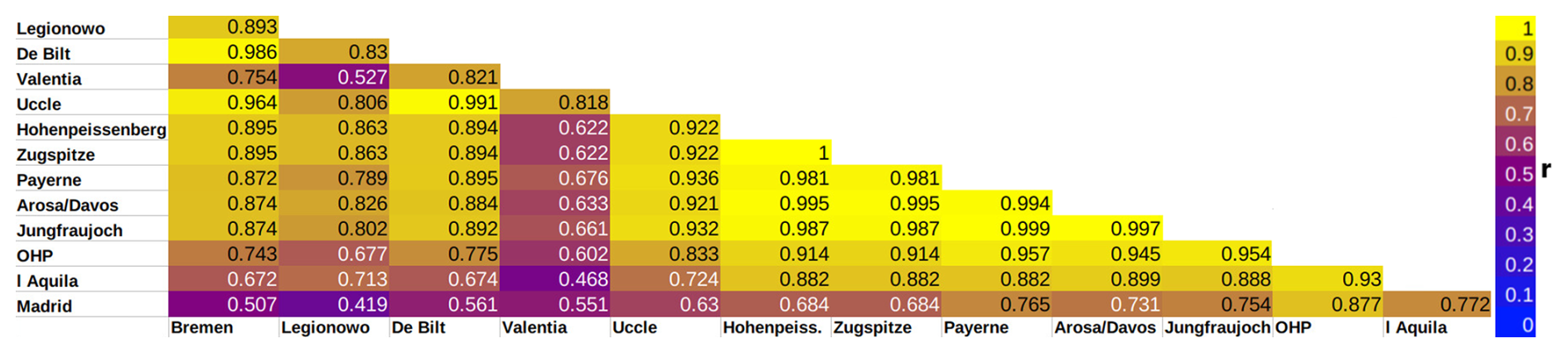
Figure 3 Correlations in the lower stratospheric partial column for Continental Europe sites. The cell colors vary from yellow to blue based on the correlation. The correlation (r) above (resp. below) 0.75 is written in black (resp. white).

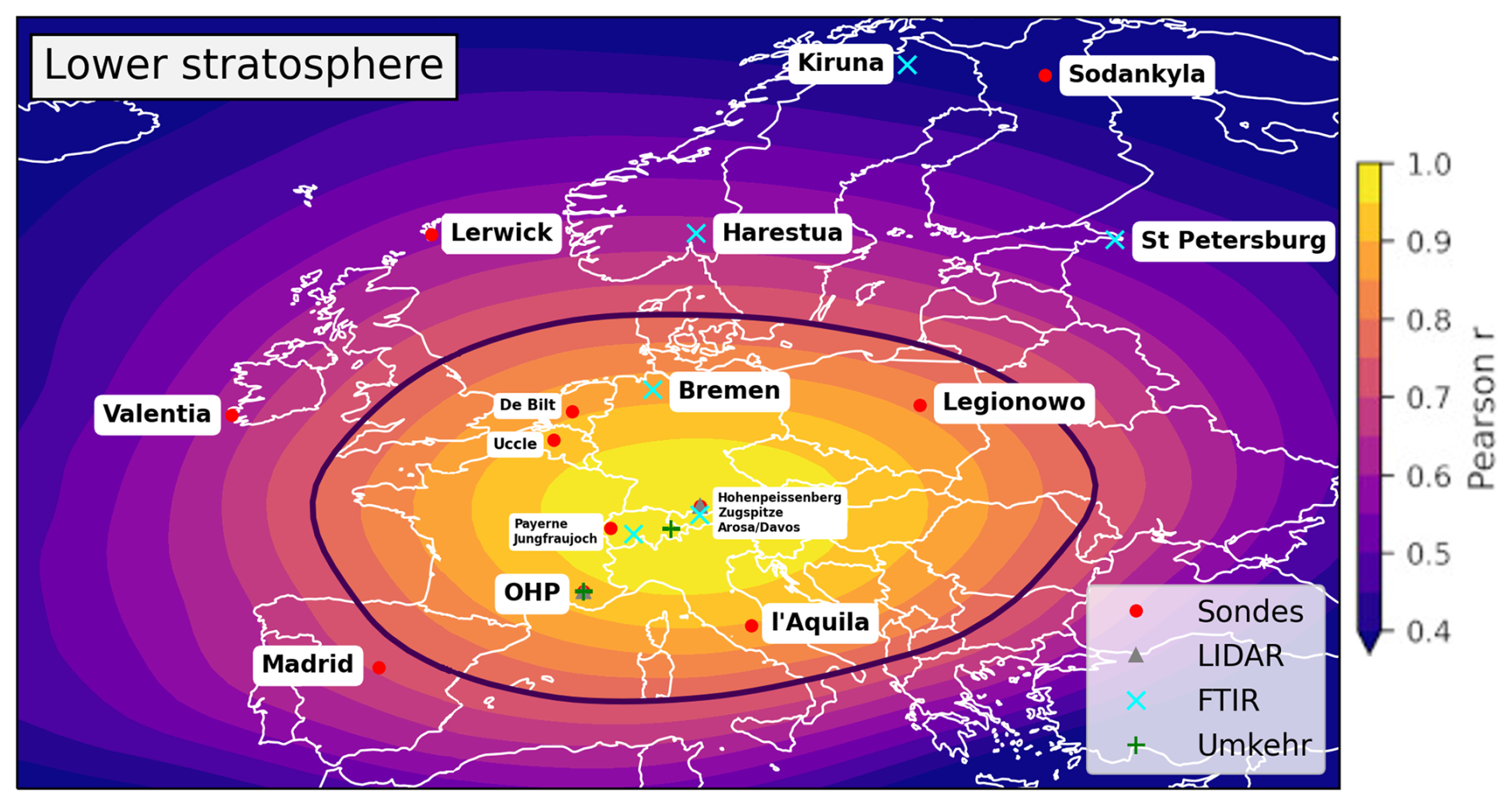
Figure 4 Correlation map for Zugspitze, FTIR (47.42° lat., 10.98° long.) in the lower stratosphere. We see that all sites in the Central Europe group lie within the r>0.75 limit (black line) of correlation with Zugspitze.

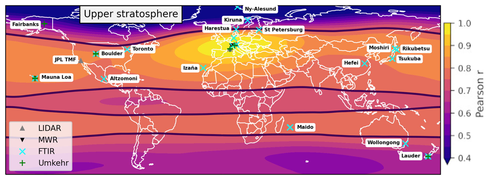
Figure 5 Correlation map for Zugspitze in the upper stratosphere. The r>0.75 region limit (black line) here spans the whole mid latitude region. In the upper stratosphere, the ozonesondes are not measuring so there are only 30 stations available there.

3.2 Composite time series

Merging heterogeneous records requires careful handling of systematic biases and outliers. In this section, we describe the pre-processing of the data records and compare two merging methodologies: the conventional weighted mean (WM) and the BAyeSian Integrated and Consolidated (BASIC) algorithm (Ball et al., 2017). The composite aims to be the best estimate of what would have been measured by a single stable instrument, with the spatial redundancy and combined temporal resolution of all the instruments in the group. It is a regional ozone timeseries with appropriate uncertainties.

3.2.1 Offset removal

Systematic errors (including offsets) might exist between ozone datasets within the same region due to local atmospheric variability and differences between retrieval techniques. To account for this, following Ball et al. (2017), we align all the time series to a common baseline. We calculate the mean value of a selected reference instrument (arbitrarily chosen) over an arbitrary reference period (2009–2014). All other series in the group are shifted (via subtraction of their respective means) to align with this reference. This process effectively removes relative offsets, resulting in a unified dataset of aligned monthly means that preserves the seasonality and long-term variability, suitable for trend analysis.

Mathematically, following the notation of Ball, for the full dataset d_t,c (n_c⋅n_t matrix where n_c is the number of instruments and n_t is the number of measurements of one instrument), we define the aligned dataset ${d^{\prime }}_{t,c}$, in which we removed the relative offsets, by adjusting the mean of each instrument c to the mean of the reference instrument ${d^{\prime }}_{t,\mathrm{ref}}$ over the reference period [t₁, t₂]:

$$\begin{array}{}\text{(1)}& d_{t,c}^{\prime }=d_{t,c}-{\displaystyle \frac{\mathrm{1}}{n}}{\sum }_{t^{\prime }=t_{\mathrm{1}}}{}_{\mathrm{2}}^t{d}_{t^{\prime },c}+{\displaystyle \frac{\mathrm{1}}{n}}{\sum }_{t^{\prime }=t_{\mathrm{1}}}{}_{\mathrm{2}}^t{d}_{t^{\prime },\mathrm{ref}},\end{array}$$

where n denotes the number of months between t₁ and t₂.

3.2.2 The Weighted Mean

One way of merging datasets is computing their WM. For a set of aligned monthly mean measurements x_i with uncertainties σ_i at a given time step t, over all the instruments c of the group, the WM is defined as:

$$\begin{array}{}\text{(2)}& \mathrm{WM}\left(t\right)={\displaystyle \frac{{\sum }_{\mathrm{c}}{w}_{t,c}{d}_{t,c}^{\prime }}{{\sum }_c{w}_{t,c}}}\text{ with }{w}_{t,c}={\displaystyle \frac{\mathrm{1}}{{\mathit{\sigma }}_{t,c}^{\mathrm{2}}}}\end{array}$$

The weights are the inverse of the squared measurement uncertainties (of L3 data in our case). The WM assumes that measurement errors are normally distributed and that all instruments provide unbiased estimates of ozone. However, the WM is highly sensitive to outliers. This is particularly problematic if an outlier instrument c at a month t has a small uncertainty: the weight w_t,c becomes disproportionately large, pulling the composite average toward the outlier value. The WM assumes the reported uncertainties result only of random normally distributed measurement errors. While the harmonization of individual datasets and our alignment of the time series supposedly removed systematic errors and biases that existed, the merging correlation threshold 0.75 accepts spatial variability, another source of inconsistency. Since the WM cannot distinguish between this spatial variability and the measurement uncertainties, it allows those outliers to bias the curve.

3.2.3 The BASIC Methodology

BASIC (Ball et al., 2017) uses Bayesian inference (as defined in Rodgers, 2000) to determine the most probable underlying ozone time series by combining the data with prior knowledge of ozone variability and a robust handling of outliers.

The Bayesian method computes the posterior probability distribution of the true ozone time series y, given the observed dataset d and a month-to-month prior M as:

$$\begin{array}{}\text{(3)}& P\left(y|d,M\right)={\displaystyle \frac{P\left(y|M\right)\cdot P\left(d|y\right)}{P\left(d|M\right)}}\end{array}$$

P(y|M) is the month-to-month prior distribution. It describes the expected change of ozone from one month to another. In Ball et al. (2017), the prior is computed from the actual datasets. Here, the prior is derived from the ML climatology (McPeters and Labow, 2012), based on Aura MLS and ozonesonde datasets, rather than from the input records themselves. This reduces direct dependence on the merged timeseries, although the prior is not fully independent. The ML prior provides a climatological month-to-month constraint, while remaining broad enough for the posterior to be mainly driven by the observations.

P(d|y), the likelihood, represents the probabilistic model of the data. To account for outliers, BASIC uses a Gaussian-mixture model (Box and Tiao, 1968). Unlike a single Gaussian, it assumes that any data point has a probability β of being an outlier with an uncertainty inflated by a factor γ. This allows the algorithm to effectively down-weight data points that deviate significantly from the regional consensus. In this work, β=0.1 and  γ=100, thus we expect 10 % of outliers, that can have a 100 times bigger variance. Figure 6 illustrates this process for the Central Europe group in LS for the months of January, May and August 2012. The black curve images the probability density function of the observations, with the merged uncertainty (instruments plus PCA uncertainties, see Sect. 3.2.4), drawn as the sum of individual instrument Gaussian distributions. The green curve represents the prior distribution derived from the ML climatology- a very large distribution because of the high variability reported in the climatology.

BASIC samples the final posterior distribution $P\left(y\right|M,d)$ using a Hamiltonian Monte Carlo (HMC, in the family of Markov Chain Monte Carlo MCMC methods), following the code in Ball et al. (2017), with the Stan package (Stan Development Team, 2024). The sampling is done on n+1 chains (where n is the number of instruments of the group), with a warmup of 5000 (burn-in length) and a sampling of 20 000.

Two convergence diagnostics were applied (automatically computed by Stan):

1. The rank normalized Gelman-Rubin diagnostic ($\widehat{R}$, Vehtari et al., 2021), which quantifies the convergence of the n+1 independent Markov chains by comparing the variance within each chain with the variance between the chains. The value is typically recommended to be less than 1.01.

2. The Effective Sample Size (ESS, Vehtari et al., 2021), which estimates the number of i.i.d. draws necessary to obtain the same standard error (since the draws in the MCMC are autocorrelated). The value is typically recommended to be at least 400.

In May 2012 (Fig. 6b), the instrument's curves are close, so the probability density is almost unimodal (Wilks, 2019). Therefore, the BASIC posterior (in blue) and the WM (in red) are very similar, BASIC being broader to account for the main large body of the distribution. In the image, the sum of instruments (black) curve is larger than the blue BASIC posterior because the black curve represents the sum of individual likelihoods, whereas the BASIC curve represents the product of the likelihoods and the prior, which naturally sharpens the probability density around the consensus value.

In January 2012 (Fig. 6a), the datasets are disparate, and BASIC identifies the larger mode and ignores the outlier (peak visible at 152 DU), producing a robust estimate closer to the cluster of consistent instruments, whereas the WM is pulled toward the outlier.

Finally, in August 2012 (Fig. 6c), the probability density splits into two distinct peaks/modes (near 100 and 108 DU). The Weighted Mean is centered at 105 DU – directly between the peaks – where the actual probability density is low. This result is physically unlikely as it represents a value supported by fewer instruments than 108 DU (right peak) or 100 DU (left peak). In contrast, BASIC's Gaussian mixture model selects the more probable peak (centered at 100 DU), effectively resolving the ambiguity rather than averaging it out. Because the standard HMC struggles to traverse low-probability valleys between isolated modes (Betancourt, 2017), the parallel chains remain localized within their respective initialized peaks. The diagnostics reflect this expected topological barrier: for the bimodal August 2012 case, we record an $\widehat{R}$ of 1.044 and an ESS of 217.3 in the Lower Stratosphere (LS), and a more severe mode separation in the Upper Troposphere Lower Stratosphere (UTLS) with an $\widehat{R}$ of 1.435 and an ESS of 21.8.

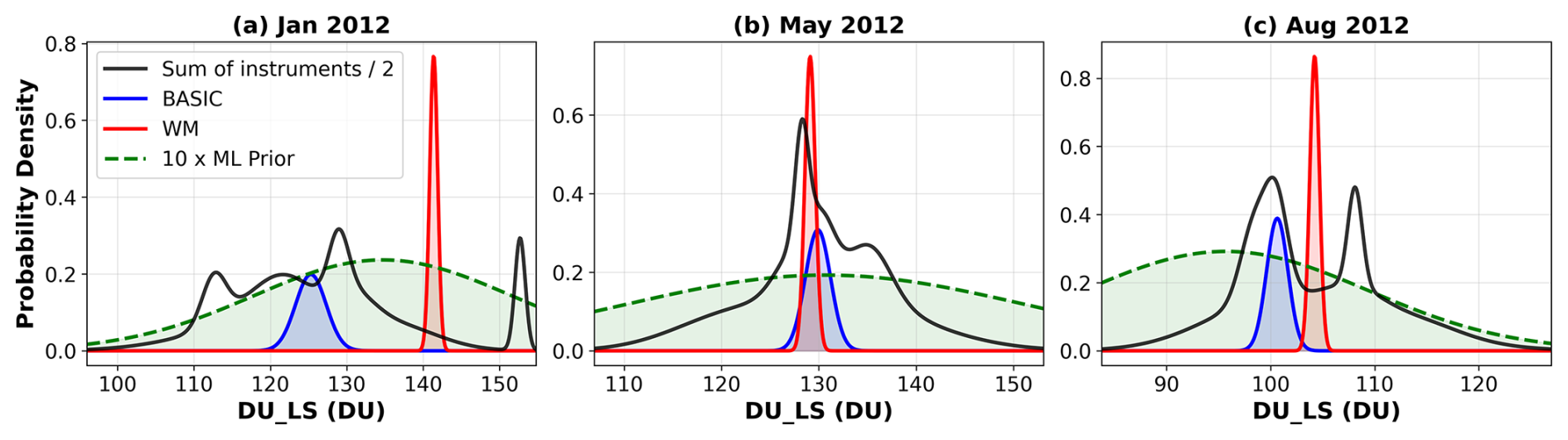
Figure 6 Illustration of the probability density sampling of BASIC, for January, August and May 2012, for the group Central Europe in LS. The black distribution is the sum of all instruments' Gaussians, the green distribution is the ML prior distribution, the blue is BASIC and the red is the WM.

3.2.4 Principal Component Analysis (PCA) uncertainties

To further enhance the detection of outliers, we use a PCA to identify the most common ozone signal among all the time series. The beta coefficient of the probabilistic model (Box-Tiao) is set to 0.1, an estimation of the proportion of outliers that becomes less robust as the number of instruments decreases. Our approach is inspired by Ball et al. (2017), except that we do not use it to create the monthly mean uncertainties (as we propagate them from the L1 data) but to improve the outliers detection. A PCA is performed via Singular Value Decomposition on the aligned datasets d^′: the first mode represents the common underlying ozone signal, while the higher-order modes represent the noise and specific variability of each timeseries. Mathematically, the decomposition of d^′ is of the form $d^{\prime }=UW{V}^T$, where U contains the temporal modes, W contains the singular values (amplitude of each mode), and V the projection coefficients (how much each temporal mode in U is present in all the instruments). The statistical uncertainty ${\mathit{\sigma }}_{\mathrm{PCA},t,i}$ for instrument i at time t is obtained by summing the contributions of the noise modes (from k=2 to N), identically to Eq. (5) in Ball et al. (2017):

$$\begin{array}{}\text{(4)}& {\mathit{\sigma }}_{\mathrm{PCA},t,i}^{\mathrm{2}}={\sum }_{k=\mathrm{2}}^N{\left(U_{t,k}{W}_{k,k}{V}_{i,k}\right)}^{\mathrm{2}}\end{array}$$

Finally, to obtain the merged uncertainties, the instrumental L3 uncertainties (σ_Profile) generally have a much larger magnitude than the statistical scatter (σ_PCA), so a direct sum is meaningless. To combine them, we use the PCA uncertainty as a scaling factor. This multiplicative scaling is applied because it proportionally inflates the propagated uncertainties of instruments that deviate from the consensus. This allows the Bayesian framework (BASIC) to smoothly down-weight outliers without discarding the underlying data. For each month, we identify the “reference” instrument as the one with the smallest statistical uncertainty (σ_PCA,ref). The final merged uncertainty used in BASIC is given in Eq. (5).

$$\begin{array}{}\text{(5)}& {\mathit{\sigma }}_{\mathrm{Merge},i}={\mathit{\sigma }}_{\mathrm{Profile},i}\cdot {\displaystyle \frac{{\mathit{\sigma }}_{\mathrm{PCA},i}}{{\mathit{\sigma }}_{\mathrm{PCA},\mathrm{ref}}}}\end{array}$$

The resulting merged uncertainties contain in the end the L3 profile uncertainties, inflated with respect to their agreement to the reference PCA uncertainty, which is the smallest PCA uncertainty for this month. We acknowledge a theoretical limitation to this methodology: by strictly down-weighting instruments that deviate from the PCA consensus, the method could, in principle, suppress genuine physical signals that are uniquely captured by a single high-resolution instrument.

3.3 Multiple Linear Regression (MLR) trend estimation

Trends are estimated using the weighted multiple linear regression (MLR) model developed within the APARC/LOTUS initiative. This open-source regression tool (v0.8.3, see Supplement Sect. S5) has been widely used for evaluating stratospheric ozone profile trends since the WMO 2018 Assessment (WMO, 2018). Here we evaluate trends between January 2000 and December 2024. The multiple regression of the time serie y(t) is performed as follows:

$$\begin{array}{}\text{(6)}& \begin{array}{rl}y\left(t\right)& ={\mathit{\beta }}_{\mathrm{1}}\left(t\right)\cdot {\mathrm{QBO}}_{\mathrm{1}}\left(t\right)+{\mathit{\beta }}_{\mathrm{2}}\left(t\right)\cdot {\mathrm{QBO}}_{\mathrm{2}}\left(t\right)+\\ & {\mathit{\beta }}_{\mathrm{3}}\cdot \mathrm{Solar}\left(t\right)+{\mathit{\beta }}_{\mathrm{4}}\cdot \mathrm{ENSO}\left(t\right)+{\mathit{\beta }}_{\mathrm{5}}\cdot \mathrm{AOD}\left(t\right)+\\ & {\mathit{\beta }}_{\mathrm{6}}\left(t\right)+{\mathit{\beta }}_{\mathrm{7}}\cdot t+\mathit{ϵ}\left(t\right)\end{array}\end{array}$$

With

$$\begin{array}{rl}{\mathit{\beta }}_i\left(t\right)& ={\mathit{\beta }}_{i,\mathrm{0}}+{\sum }_{k=\mathrm{1}}^{\mathrm{2}}{\mathit{\beta }}_{i_{\mathrm{1}},k}\sin \left({\displaystyle \frac{\mathrm{2}\mathit{\pi }kt}{\mathrm{12}}}\right)+\\ & {\sum }_{k=\mathrm{1}}^{\mathrm{2}}{\mathit{\beta }}_{i_{\mathrm{2}},k}\cos \left({\displaystyle \frac{\mathrm{2}\mathit{\pi }kt}{\mathrm{12}}}\right)\text{ for }i=\mathrm{1},\mathrm{2},\mathrm{5}.\end{array}$$

The trend estimation is performed here directly on the monthly mean composite time series, and the annual cycle is modeled within the regression by expanding specific coefficients (the intercept β₆(t) in Eq. 6) into Fourier series. Moreover, the merging methods provide uncertainties for their monthly mean values, which enable the use of a weighted MLR. The fit is constrained by the inverse of the squared BASIC uncertainties ($\frac{\mathrm{1}}{{\mathit{\sigma }}_{\mathrm{BASIC}}^{\mathrm{2}}}$), so that months with smaller uncertainties – therefore higher confidence – contribute more to the trend result.

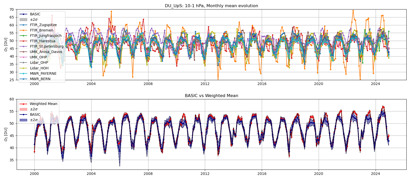
Figure 7 Time series for regional group central Europe, in the Upper Stratosphere (UpS). Top: time series of the group members, plotted with BASIC in blue and its uncertainty in grey. Bottom: comparison between BASIC in blue, with 2 uncertainties in blue, and the Weighted mean in red, with 2 uncertainties in red.

The other functions in Eq. (6) are the explanatory variables, which have been chosen to be the same for all the regional groups to make the inter-regional comparison easier:

• QBO: The Quasi-Biennial Oscillation is modeled using two orthogonal components (EOF-1 and EOF-2) derived from the Principal Component Analysis of Singapore stratospheric winds (10–100 hPa).

• Solar Cycle: The 11-year solar cycle is represented by the 10.7 cm solar radio flux (F10.7).

• ENSO: El Nino Southern Oscillation.This is the proxy used in previous LOTUS papers such as Godin-Beekmann et al. (2022). ENSO modulates stratospheric ozone through fluctuations in the tropical upwelling of the Brewer-Dobson circulation (Randel et al., 2009).

• sAOD: Aerosol Optical Depth from GloSSAC v2.2 (Thomason et al., 2018) to account for volcanic perturbations (e.g., Raikoke, Hunga Tonga) and ozone chemistry.

The linear trend is the coefficient β₇ in DU per month, which can then be converted into % per decade using the climatological mean. The uncertainty of the trend estimates (σ_Trend) is derived from the standard error of the regression coefficient β₇. However, the autocorrelation in the fitting residuals (ϵ(t)) typically leads to underestimated uncertainties. To correct this, we apply the Cochrane-Orcutt transformation (Cochrane and Orcutt, 1949) to remove first-order autocorrelation from the residuals.

Figure 8 Same as Fig. 7 for the Middle Stratosphere (MS).

Figure 9 Same as Fig. 7 for the Lower Stratosphere (LS).

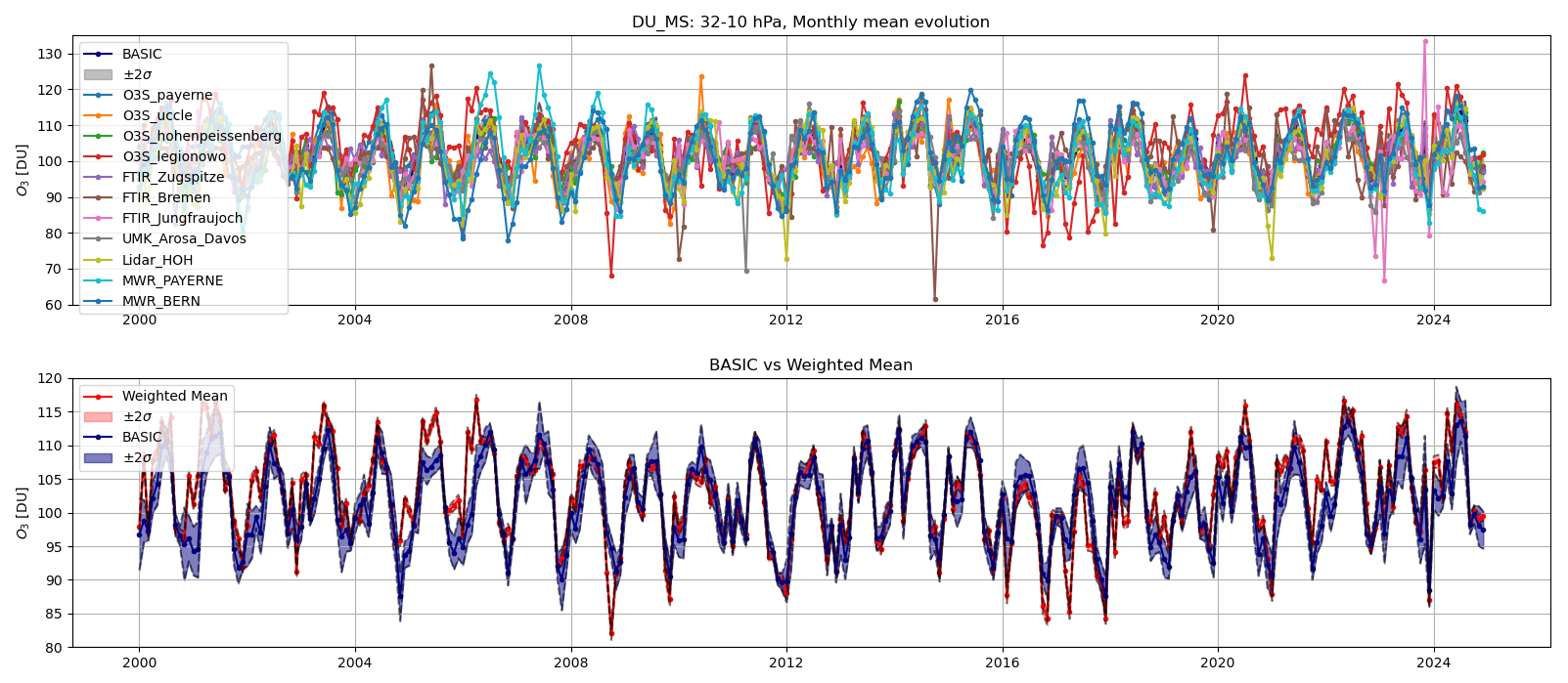
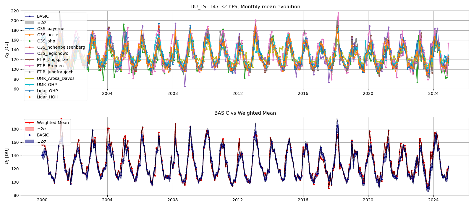
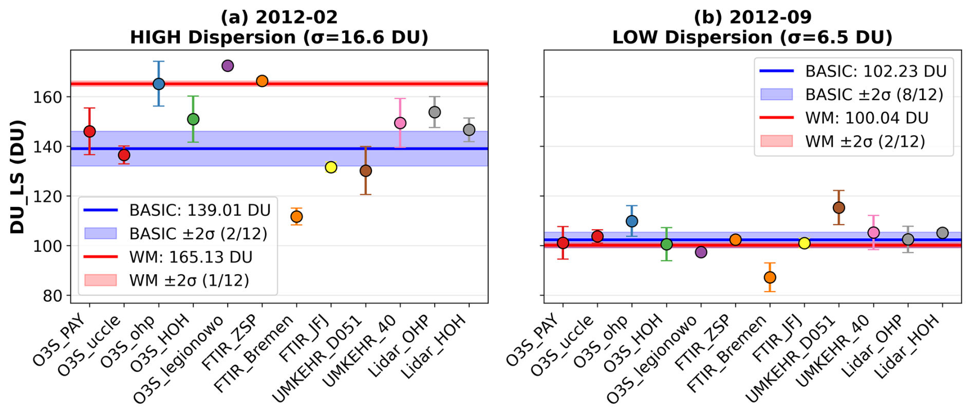
Figure 10 Monthly mean ozone values in DU for all the instruments in the group Central Europe in LS, for two months selected for their high (left panel, February 2012) and low (right panel, September 2012) variability. The BASIC (in blue) and WM (in red) composites are superposed with their 2σ uncertainties.

The quality of the regression fit is assessed using the Adjusted Coefficient of Determination ($R_{\mathrm{adj}}^{\mathrm{2}}$). Unlike the standard R², which increases automatically with the number of predictors, $R_{\mathrm{adj}}^{\mathrm{2}}$ accounts for the degrees of freedom:

$$\begin{array}{}\text{(7)}& R_{\mathrm{adj}}^{\mathrm{2}}=\mathrm{1}-(\mathrm{1}-R^{\mathrm{2}})(n-\mathrm{1})/(n-p-\mathrm{1})\end{array}$$

where n is the number of observations and p is the number of predictors. A high $R_{\mathrm{adj}}^{\mathrm{2}}$ (closer to 1) indicates that the chosen proxies and seasonal model successfully capture the observed ozone variability. On the other hand, a low $R_{\mathrm{adj}}^{\mathrm{2}}$ suggests that the variability is driven by processes not included in the model (e.g., chaotic dynamical noise in the lower stratosphere), or that the instrumental noise exceeds the natural variability. Trends are considered statistically significant at the 95 % confidence level if their absolute value exceeds their 2σ uncertainty (if | Trend $|>\mathrm{2}{\mathit{\sigma }}_{\mathrm{Trend}})$.

4 Results and Discussion

4.1 BASIC composites

The BASIC methodology was applied to all the regional groups of datasets that are described in Tables S2–S5 (see Supplement Sect. S2). Here, we display the group Central Europe as a representative case study to compare the performance of BASIC with the conventional WM. Figure 7 displays the time series in UpS. The aligned individual time series (top panel) show a seasonal cycle ranging generally between 40 and 60 DU, with individual outliers ranging from 30 to 70 DU. In this layer, there are no particular discrepancies between BASIC (in blue) and WM (in red) composites (bottom panel). The differences between the two methods are minimal, indicating that when the underlying data are consistent, either composite method converges to the standard result. The visible extremes in individual records are likely outlier measurements rather than systematic differences in annual cycle amplitude, and are down-weighted by the merging in BASIC rather than removed by the offset correction.

In Fig. 8, corresponding to MS, the annual variability ranges from 80 to 110 DU. Divergences between the merging methods are visible, e.g. in 2005–2006, where the WM is consistently higher than BASIC during almost 2 years. This is driven largely by the O3S Legionowo (and other ozonesondes), which are significantly higher than the other instruments during this period. BASIC remains centered on the majority of the instruments, but with a larger uncertainty to include the larger range of variability. In 2017–2018, the opposite occurs: O3S Legionowo (and other ozonesondes) are lower than the rest, dragging the WM downward. Finally, during the beginning and the end of the time series, the instrumental variability is large, and BASIC uncertainties reflect the lack of consensus by being larger. In contrast, the WM uncertainties remain unrealistically small, failing to capture the structural variability at this month.

In Fig. 9, in LS, we observe the largest dispersion, ranging from 90 to 175 DU, with outliers extending from 60 to 210 DU. While the BASIC and WM time series often overlap, their uncertainty characterization differs fundamentally. Figure 10 compares individual instrument monthly means with the BASIC and WM composites and their ±2σ uncertainty intervals. Mathematically, the BASIC algorithm assumes a Box–Tiao error distribution (with outlier proportion β=0.1 and variance inflation γ=100). In such a distribution, one expects 92 % of the data to be included within the ±2σ uncertainty intervals, and 99.7 % of the data for a pure Gaussian. In Fig. 10a (February 2012), the instrument values are widely scattered (105–165 DU). The BASIC algorithm accounts for this dispersion with a large posterior uncertainty: the BASIC ±2σ interval includes 5 out of 12 instruments. The WM ±2σ interval, however, is extremely narrow, overlapping with only 1 of 12 instruments. In Fig. 10b (September 2012), where agreement is better (80–110 DU), the BASIC uncertainty interval is smaller and overlaps with 8 of 12 instruments. The WM ±2σ interval overlaps with 2 of 12 instruments. These results are to be interpreted cautiously because the time series are correlated and biases may exist. These coverage counts are only illustrative; however, they clearly highlight the robustness of the Bayesian error inflation to deal with outliers compared to the conventional WM.

Finally, Fig. S1 presents the Tropospheric partial column. Despite periods of high instrumental variability (e.g., March 2004, where BASIC uncertainty exceeds 10 DU to account for the inter-instrument spread), the overall time series of BASIC and the WM overlap significantly. This agreement confirms that BASIC is robust enough to retrieve the regional ozone variability shared across all instruments in the group, even in the most heterogeneous layer of the atmosphere, with the remaining variability left as unexplained noise. The distinct advantage of BASIC lies in its uncertainty characterization: it accounts for periods of low consensus with large uncertainties, whereas the WM ignores it.

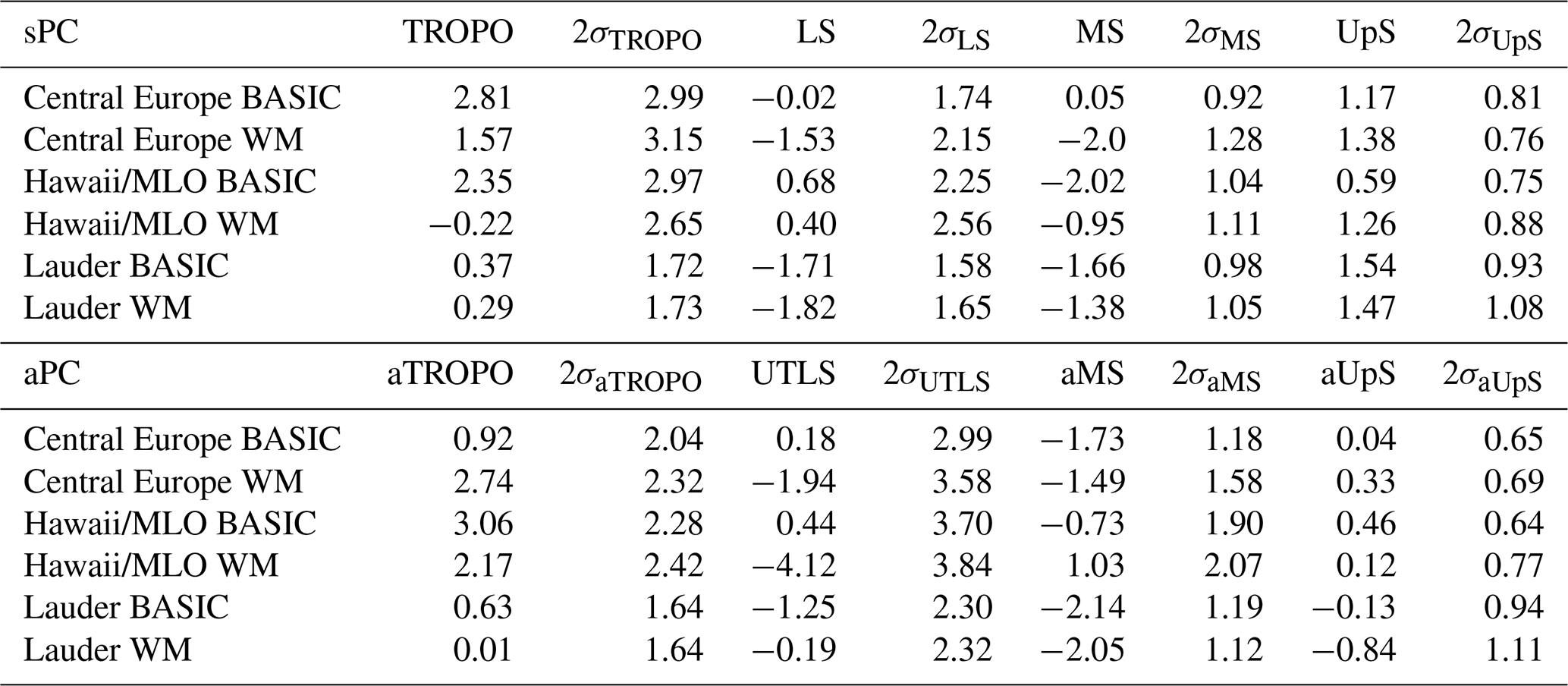
Table 2 BASIC and WM trends and trend uncertainties in % per decade for three selected NDACC stations, for sPC and aPC. In bold are significant trends and their uncertainty.

4.2 Vertical regional trends

The trends for the 2000–2024 period are estimated using the LOTUS version 0.8.3 regression model described in Sect. 3.3. We illustrate the results here for three groups of selected NDACC stations: the mid-latitude Central Europe, Mauna Loa (MLO) in the tropics, and Lauder in the Southern-Hemisphere, as investigated in Godin-Beekmann et al. (2022) for the period 2000–2020 and Sofieva et al. (2026) for the period 2000–2024, but results are provided for all regions and all layers in Sect. 4.3. In the figures of this section (e.g. Fig. 11), the legend lists the datasets for which the trends have not been estimated on the same time range as the composite trends period, either beginning later than 2000, or finishing before 2024, and/or which have significant data gaps. The complete list of time range and gaps for each instrument is available in Table S1. A common misconception is to consider that the weighted mean trend is a weighted mean of the trends of the individual instruments. It would hold only if the commutator between the operator of merging (BASIC or the weighted mean) and the operator of trend estimation (MLR) would be 0. Because of the reduction of dimensionality in the merging techniques (from n timeseries to 1) and in the MLR (from more than 220 monthly mean to 2 values), this commutator is likely different from 0, which means the trends from the composites cannot be considered as the mean of the individual trends. We chose to include individual trends to illustrate the reduction of the uncertainty allowed by the merging techniques. In Table 2, we display the estimated trends for the two sets of partial columns sPC and aPC, for the two merging techniques and for three selected regions (Europe, Hawaii and Lauder). BASIC trend uncertainties are systematically smaller than those of the WM (except in the group Hawaii in TROPO). Over these groups, BASIC uncertainties are on average 9.4 % smaller than the WM's ($=\frac{{\mathit{\sigma }}_{\mathrm{BASIC}}-{\mathit{\sigma }}_{\mathrm{WM}}}{{\mathit{\sigma }}_{\mathrm{WM}}})$. For Central Europe, we compute an average reduction of 15.2 % in sPC, 18.6 % in aPC, for Hawaii, 5.3 % in sPC and 8.6 % in aPC, and for Lauder 6.3 % in sPC and 2.5 % in aPC.

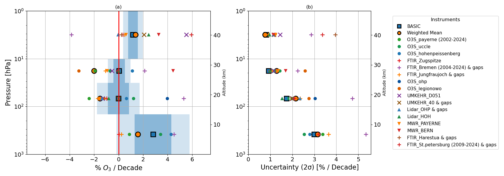
Figure 11 Trend estimates for the sPC of the regional group “Central Europe” in (a) 2000–2024 trends in % per decade. BASIC trend values are a blue square with black contour, with 1σ uncertainty in dark blue shading and 2σ in lighter blue shading. The WM trend is an orange circle with black contour. Trends for each individual dataset involved in the merged composite are plotted for comparison. (b) 2σ uncertainties of the composites and of each dataset are shown in % per decade. The legend highlights datasets with time ranges deviating from the 2000–2024 time period and/or with substantial gap.

Figure 12 Same as Fig. 11 for the aPC of the group “Central Europe”.

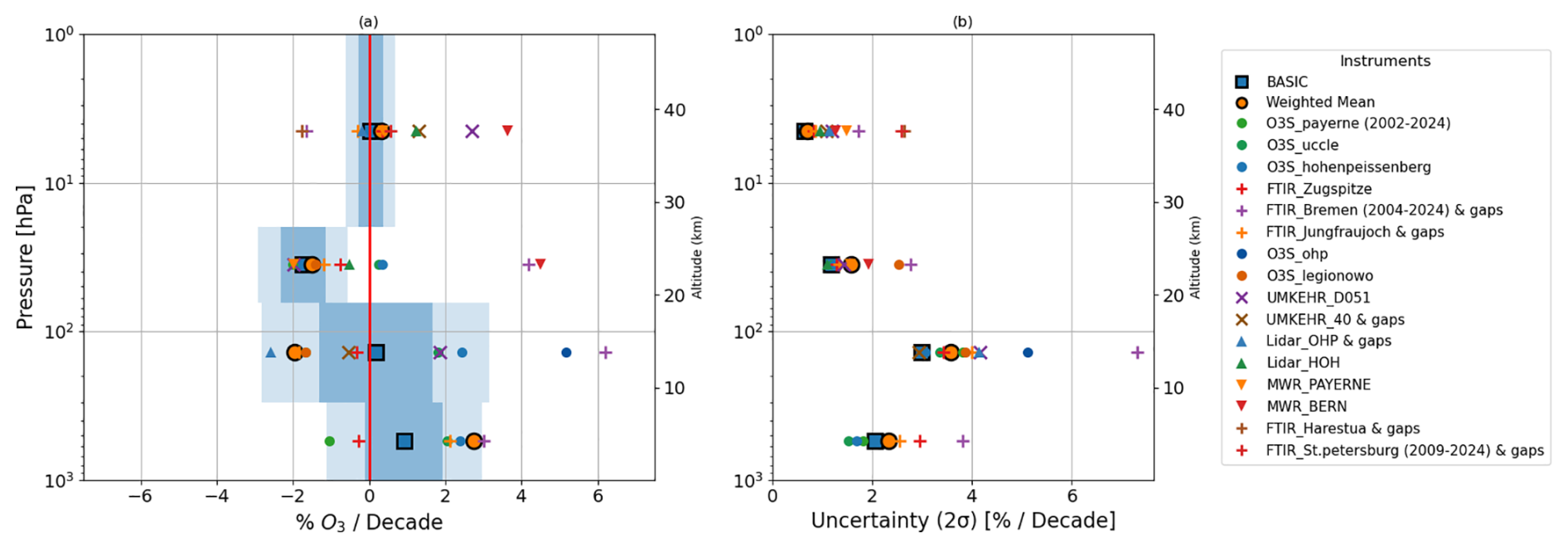
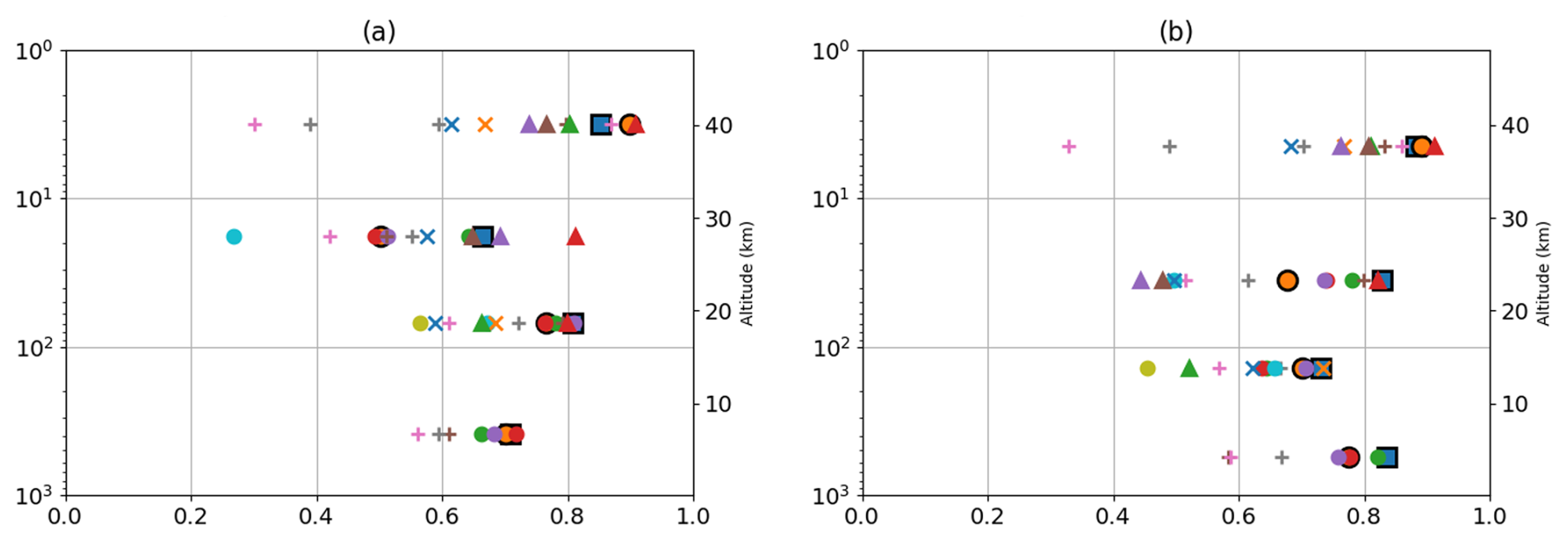
Figure 13 Adjusted R² for BASIC, the weighted mean and the datasets of the Central Europe group for (a) sPC and (b) aPC.

Table 2 allows a direct comparison between the sPC and aPC trend estimates. The two sets allow to provide a vertically coherent picture of the trend profile. For Central Europe, the MS trend of 0.05 ± 0.92 % per decade (BASIC) is non-significant, while the aMS yields −1.73 ± 1.18 % per decade (significant at the 2σ level) suggesting that the MS layer is contaminated by dynamical noise near the tropopause, consistent with the residual diagnostics discussed in Sect. 3. For Lauder and Hawaii, both MS and aMS are significant, but the aMS uncertainties are larger, given the lower altitude of the aMS layer. From LS to UTLS, the UTLS systematically shows larger uncertainties and smaller trend magnitudes than the LS, as the inclusion of the upper troposphere dilutes the stratospheric signal. Taken together, the sPC and aPC layers reconstruct a physically consistent vertical trend profile: positive in the upper stratosphere, negative in the middle and lower stratosphere, and positive in the troposphere, the expected signature of stratospheric ozone recovery.

4.2.1 Central Europe

Figures 11 and 12 display the trends over Central Europe for the two sets of partial columns, sPC and aPC respectively. Individual dataset trends show substantial scatter (considering only the instruments' trends with complete period, see Table S1 for data availability) and are shown as diagnostic context only, not interpreted as independent estimates of the same regional trend. The regional interpretation is based on the trend estimated from the merged composite. The BASIC and WM trend composites generally align. The adjusted R² values (Fig. 12) are systematically higher for the composite trends than for individual record trends, therefore justifying the merging/composite approach.

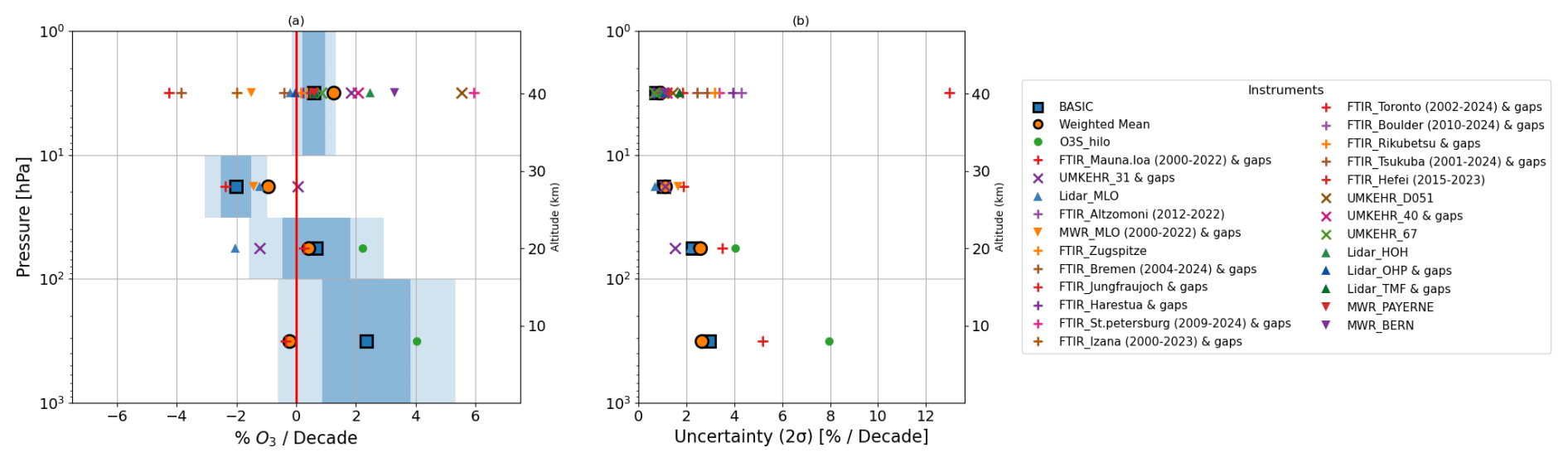
Figure 14 Trend estimates for the sPC of the regional group Hawaii. (a) 2000–2024 trends in % per decade. BASIC trend values are a blue square with black contour, with 1σ uncertainty in light dark shading and 2 sigma in lighter blue shading. The WM trend is an orange circle with black contour. Trends for each individual dataset involved in the merged composite are plotted for comparison. (b) 2σ uncertainties of the composites and of each dataset are shown in % per decade. The legend highlights datasets with time ranges deviating from the 2000–2024 time period and/or with substantial gap.

Figure 15 Same as Fig. 14 for the aPC of the group Hawaii.

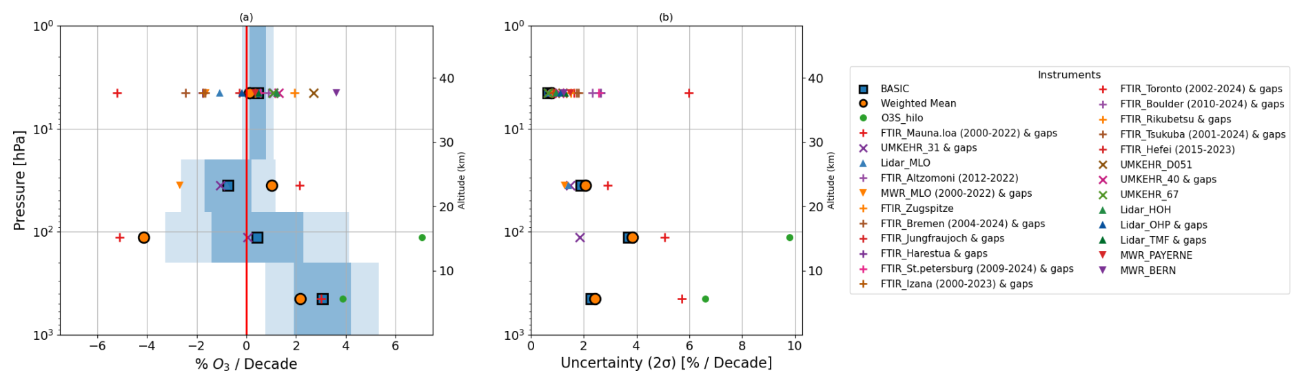
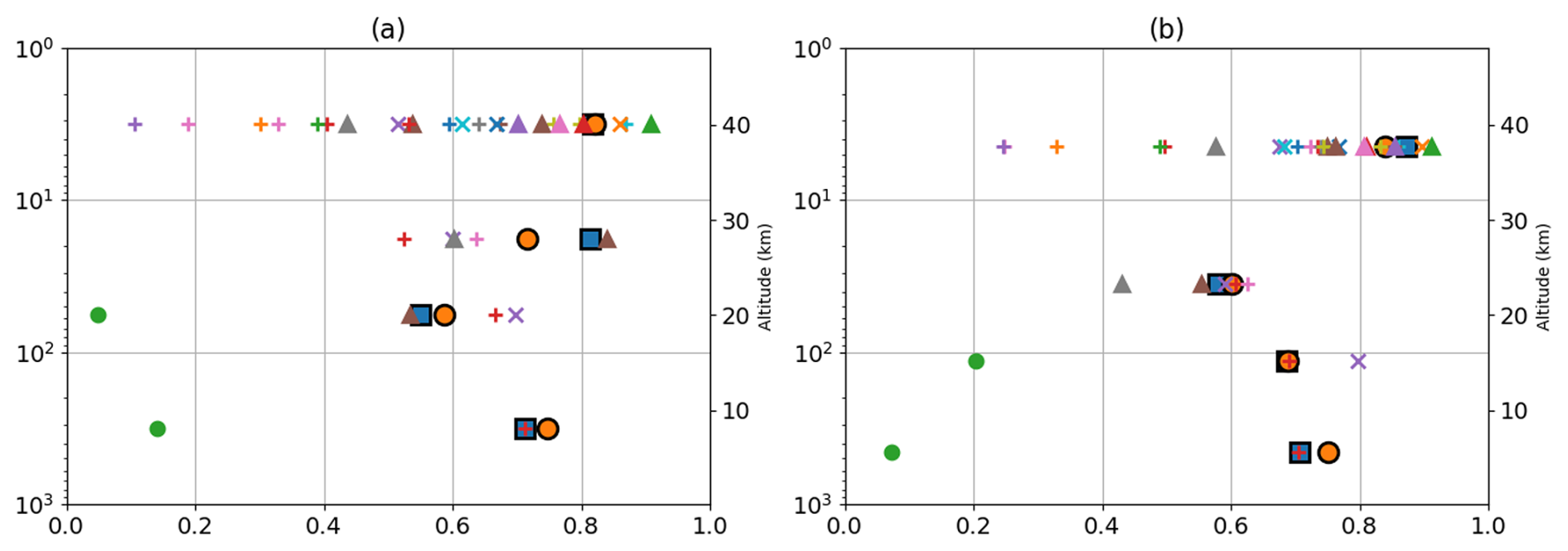
Figure 16 Adjusted R² for BASIC, the weighted mean and the datasets of the Hawaii group for (a) sPC and (b) aPC.

In the Upper Stratosphere (UpS, 10–1 hPa), trends are positive and significant (+1.17 ± 0.81 % per decade). Both the Middle Stratosphere (MS) and lower Stratosphere (LS) show near-zero trends for BASIC. On the other hand, the WM's trends in the Middle Stratosphere and Lower Stratosphere (LS) are negative, significant in MS. The trend uncertainties for the BASIC composite are systematically smaller than those of the WM and of individual datasets. For the alternative partial columns (aPC, Fig. 12), in the aUpS, BASIC (+0.04 ± 0.65 % per decade) and the WM (+0.33 ± 0.69 % per decade) are both non-significant, though BASIC gives smaller uncertainties. The aMS layer is aligned for both methods, with negative trends (significant for BASIC). In UTLS, the WM finds a strongly negative trend (−1.94 ± 3.58 % per decade) whereas BASIC reveals null trends. Both methods deliver large uncertainties for this dynamical layer. The aPC definition allows the variability of the UTLS signal to be isolated in a single layer, while this is smoothed out in the standard LS partial column. Finally, the aTROPO trends are small and non-significant for BASIC, contrasting with the positive significant trend obtained with the WM. Both sets of partial columns report significant differences between BASIC's trends and the WM's ones, particularly in the mid-low Stratosphere.

Our results align well with Sofieva et al. (2026), who report trends over the period 2000–2024 for Alpine Stations (Central Europe) in their Fig. 6c. Note that in Sofieva et al. (2026), the merging is done after the trend estimation and that we compare highly resolved vertical trends to partial column trends. We report a transition from significant positive trends in the UpS to near-zero trends in the LS, consistent in direction with the negative trends reported by Sofieva et al. (2026), Godin-Beekmann et al. (2022) and Petropavlovskikh et al. (2025). In UTLS, we report a near-zero trend (0.18 ± 2.99 % per decade). The absence of significance in the LS likely reflects the dilution of the negative signal near 100 hPa reported by Sofieva et al. (2026). The aMS layer (64–20 hPa) reports a significant negative trend (−1.73 ± 1.18 % per decade) in contradiction with other results reported in literature. The inversion height can be defined by the point where the negative trends become positive (or vice versa). Petropavlovskikh et al. (2025) suggest an inversion height in the 20–10 hPa region. Our data supports this, as the aMS (64–20 hPa) is significantly negative while the MS (32–10 hPa) is null. Finally, we report positive non-significant trends in the troposphere consistent with Van Malderen et al. (2025b). Note that the trend estimation method, the considered regions and the merging method are different in both studies, and we have considered the estimation of tropospheric trends to be beyond the scope of this study.

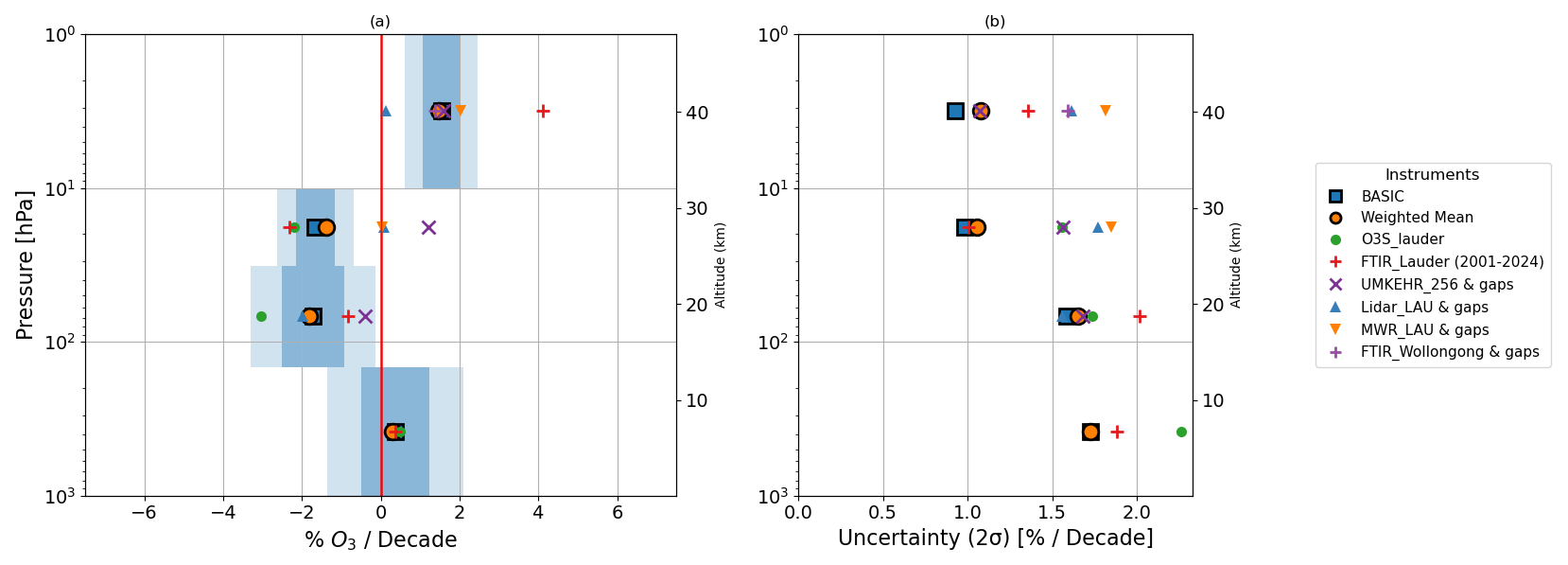
Figure 17 Trend estimates for the sPC of the regional group Lauder. (a) 2000–2024 trends in % per decade. BASIC trend values are a blue square with black contour, with 1σ uncertainty in dark blue shading and 2σ in lighter blue shading. The WM trend is an orange circle with black contour. Trends for each individual dataset involved in the merged composite are plotted for comparison. (b) 2σ uncertainties of the composites and of each dataset are shown in % per decade. The legend highlights datasets with time ranges deviating from the 2000–2024 time period and/or with substantial gap.

Figure 18 Same as Fig. 17 for the aPC of the group Lauder.

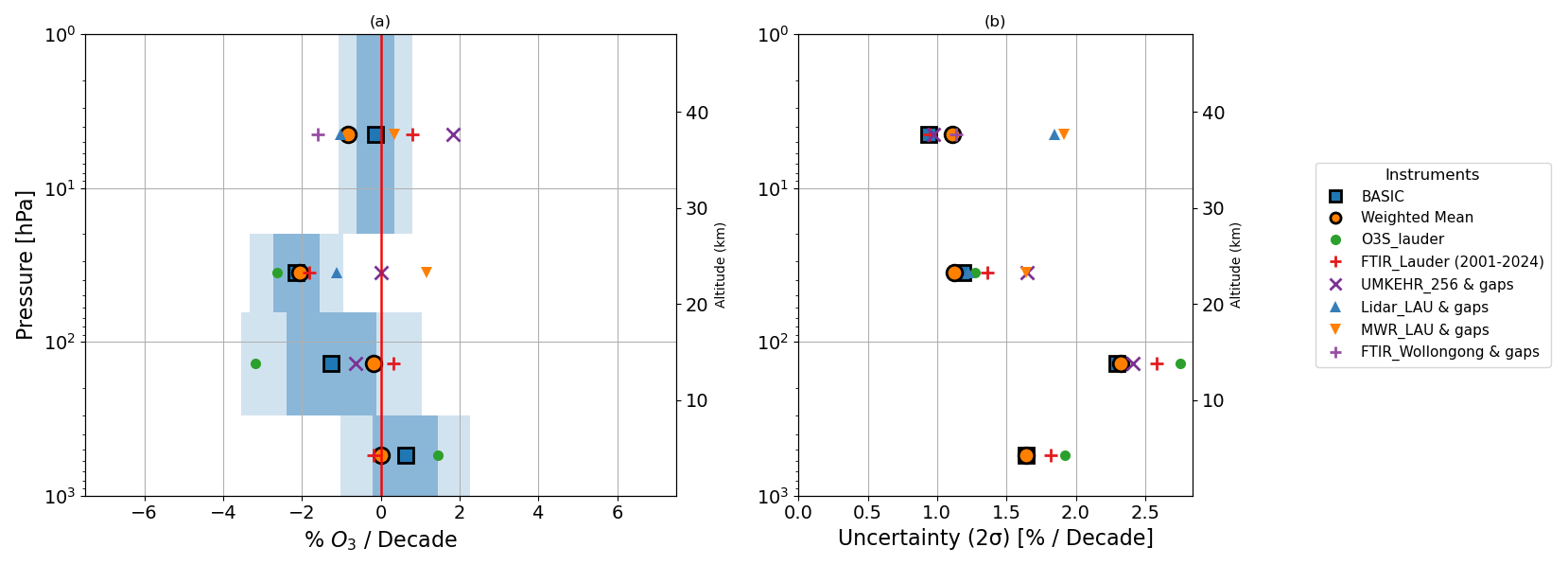
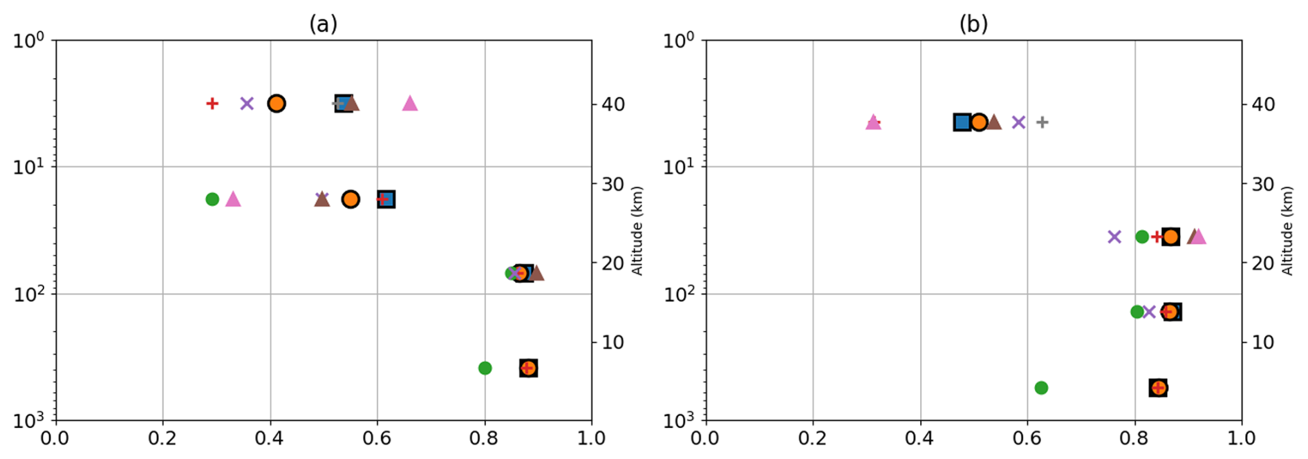
Figure 19 Adjusted R² for BASIC, the weighted mean and the datasets of the Lauder group for (a) sPC and (b) aPC. Legends are similar to those of Figs. 17 and 18.

4.2.2 Hawaii/Mauna Loa (MLO)

Figures 14 and 15 display the trends for the Hawaii region (see Table 2 for values). The UpS partial column is the broadest “Mid-Latitudes” group (24+ instruments), while lower partial columns rely on the MLO specific datasets (disparate geographical spread, see Tables S2–S5). In the Upper Stratosphere (UpS in sPC), both the BASIC and WM methods reveal positive trends (BASIC: +0.59 ± 0.75 % per decade). On the other hand, in MS (sPC), BASIC shows statistically significant negative trends (BASIC: −2.02 ± 1.04 % per decade). In LS (sPC), the observed near zero trends lack statistical significance (BASIC: +0.68 ± 2.25 % per decade) with a large uncertainty explained by low adjusted R²<0.6, see Fig. 16. Finally, BASIC demonstrates positive trends in the troposphere (BASIC: +2.35 ± 2.97 % per decade), severe disagreement with the WM (−0.22 ± 2.65 % per decade). In summary, BASIC composite exhibits systematically smaller uncertainties across all partial columns than the WM, except for the standard TROPO where they are comparable but smaller for the WM (BASIC 2.97 % per decade vs. WM 2.65 % per decade).

For the alternative partial columns (aPC), discrepancies arise in aMS, where BASIC estimates a negative trend (−0.73 ± 1.90 % per decade) while the WM suggests a positive one, though neither is statistically significant and both exhibit low adjusted R² (< 0.6). The individual instruments are diverging from the very positive FTIR to the very negative MWR, both with incomplete period (2000–2022) and gaps. In UTLS, BASIC indicates positive trends (BASIC: +0.44 ± 3.70 % per decade) opposed to the extreme negative WM's trends (−4.12 ± 3.84 % per decade), but these are associated with large uncertainties and low adjusted R² (< 0.7), though better than in LS. In contrast, the UpS and aUpS layers exhibit a high trend reliability with adjusted R²>0.8.

Our results diverge from the literature in the layers below UpS. Sofieva et al. (2026) report slightly positive UpS trends transitioning to negative trends in the tropical UTLS. In contrast, our analysis gives positive non-significant UTLS trends. This discrepancy may be partially attributed to the inclusion of the Mauna Loa FTIR record in our analysis, which is absent from the Sofieva et al. (2026) study. The FTIR record is temporally sparse (with significant gaps in 2001–2005 and 2011) and leads to unreliable individual trend estimates, which was the main reason on why it was not used in Sofieva et al. (2026). However, the BASIC methodology allows us to retain its physical information while properly weighting its uncertainties, potentially modifying the regional signal in the LS/UTLS. Furthermore, our observation of significantly negative trends in the MS contrasts with the generally zero or positive trends reported in the subtropics by Sofieva et al. (2026). This negative signal is likely influenced by the ozonesonde records, as noted by Sofieva et al. (2026). Note that the HILO ozonesonde time series shows a total column ozone drop-off since approximately 2015. This decline is described in literature as an instrumental artifact rather than a physical atmospheric change (Stauffer et al., 2020).

4.2.3 Lauder

Figures 17 and 18 display the trends for the Lauder group (values in Table 2). In the UpS, both composites show statistically significant positive trends, with BASIC estimating a recovery of +1.54 ± 0.93 % per decade. Similarly, in the MS and LS, the trends are negative and statistically significant across both methods (BASIC LS: −1.71 ± 1.58 % per decade; MS: −1.66 ± 0.98 % per decade). The robustness of the BASIC composite in these layers is further supported by the adjusted R² values shown in Fig. 19, which are consistently higher for the merged dataset compared to individual records.

However, disagreement emerges in the UTLS region: the BASIC composite indicates a negative, though non-significant, trend (−1.25 ± 2.30 % per decade, non-significant), whereas the WM suggests a near-zero trend (−0.19 ± 2.32 % per decade, non-significant). Our results in the lower stratosphere are highly consistent with Björklund et al. (2024) and Zeng et al. (2024), who both report significant negative trends for the 2000–2020 period in LS (maximal near 20 km in Björklund et al., 2024). The transition from positive trends to negative trends in the upper to middle stratosphere is further confirmed by our aUpS (20–1 hPa) trend (−0.13 ± 0.94 % per decade, non-significant), which is statistically non-significant and near zero, aligning with Zeng et al. (2024) finding of a shift from positive trends to negative trends above 30 km.

A trend distinction emerges in the LS compared to Sofieva et al. (2026). While they report negative but non-significant trends for this region, our BASIC composite produces significant negative trends in the LS with high reliability (adjusted R²>0.8 in Fig. 19). Since the WM is also negative and significant here, it suggests that it is the partial column definition that primarily enables the detection of a significant signal, while other vertical ozone profiles do not give significant trends. Finally, in the troposphere, both the standard (TROPO) and alternative (aTROPO) PC reveal positive but non-significant trends (+0.37 ± 1.72 % per decade and +0.63 ± 1.64 % per decade, respectively). These results align with those reported by Van Malderen et al. (2025a, b), Zeng et al. (2024) and Björklund et al. (2024). The slightly more positive trend in the aTROPO compared to the standard TROPO is consistent with the trend profile shape described by Zeng et al. (2024), where positive trends peak near 5 km, and suggests the influence of the UTLS in the layer TROPO, pulling towards more negative trends.

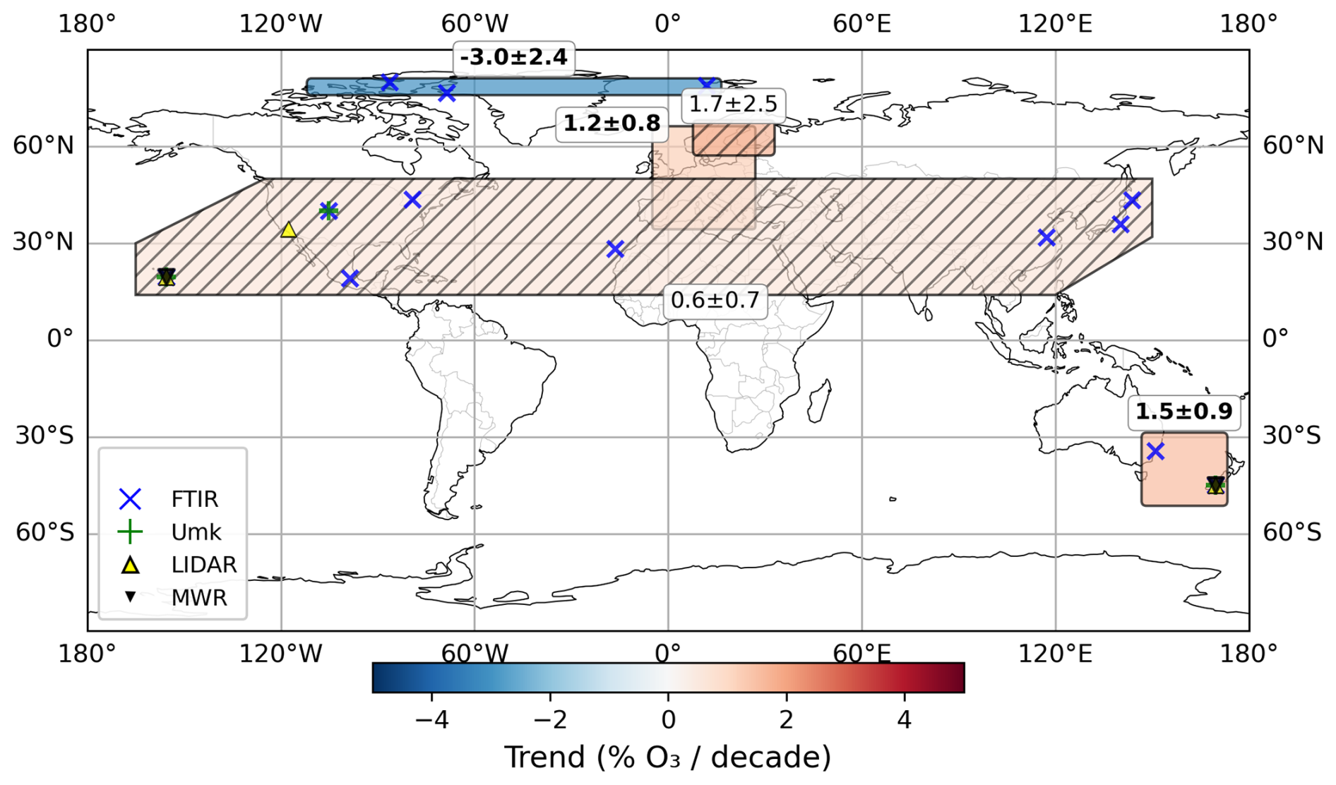
Figure 20 Ozone trends for the regional groups in the Upper Stratosphere (UpS). Bold numbers indicate significant trends. The colour scale indicates the trend magnitude: red for positive and blue for negative values. Regions are hatched where trends are not significant at the 95 % confidence level (2σ). The locations of the instruments merged into the composite are indicated by markers, except in Europe for readability.

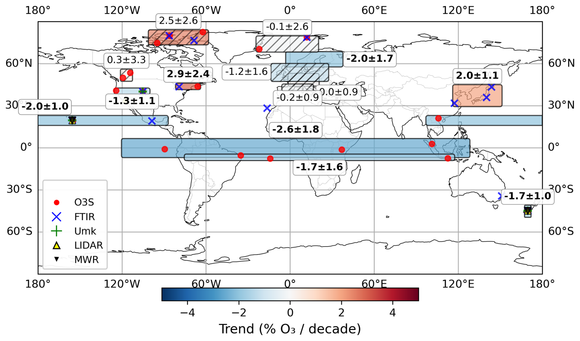
Figure 21 Same as Fig. 20 for layer MS.

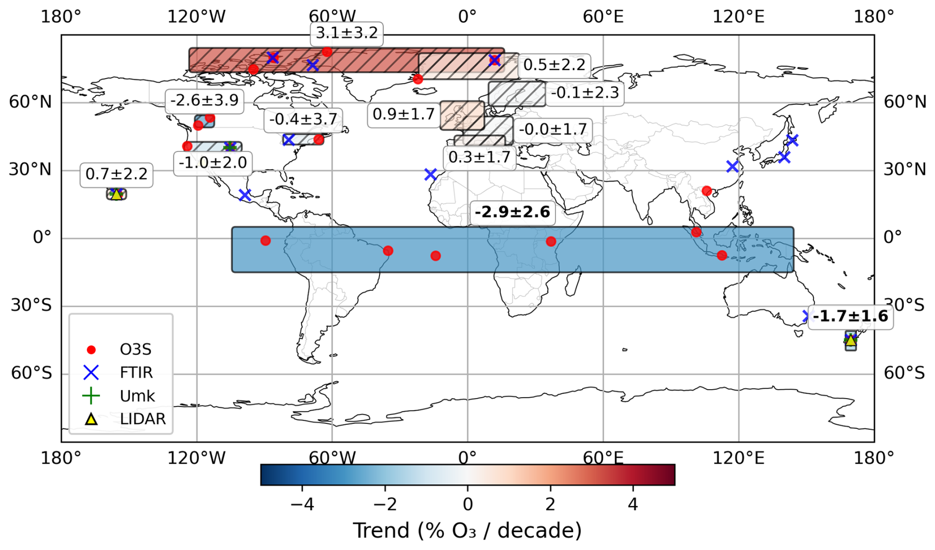
Figure 22 Same as Fig. 20 for layer LS.

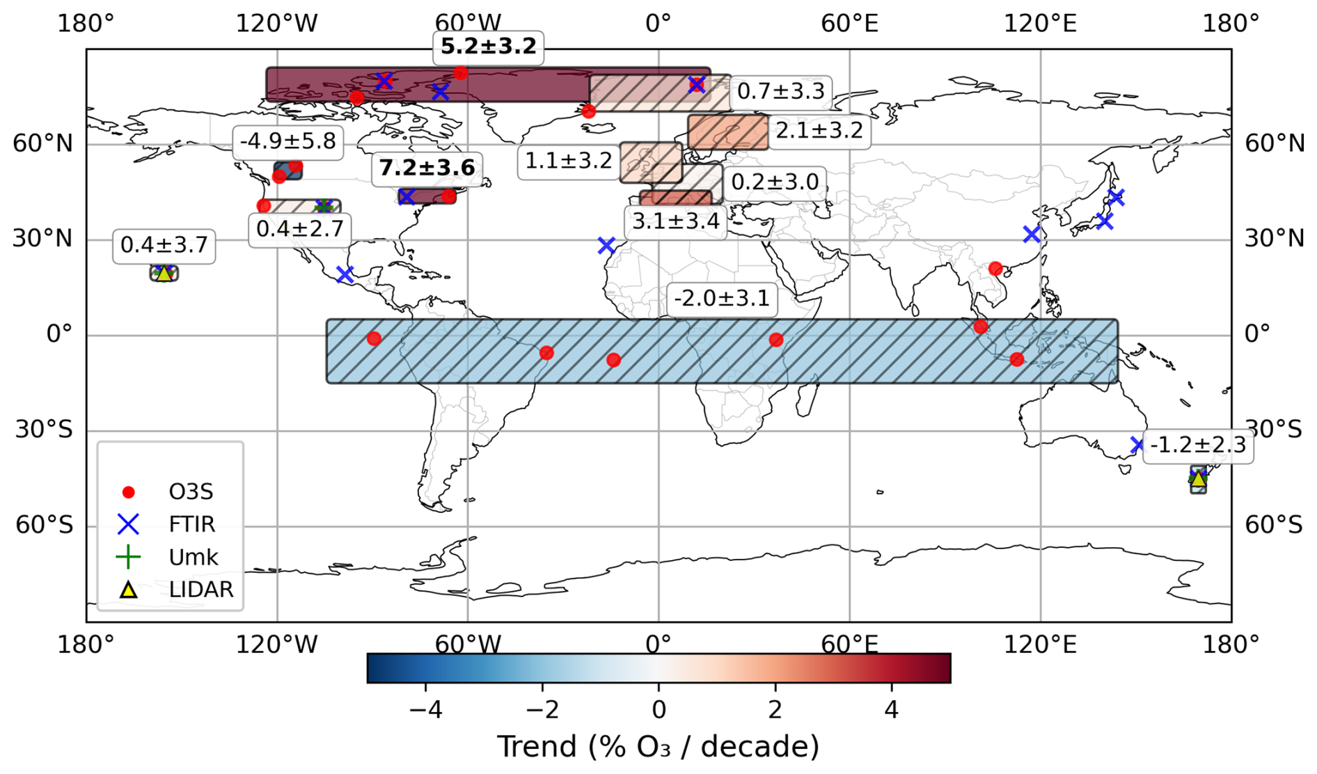
Figure 23 Same as Fig. 20 for layer UTLS.

4.3 Global maps of trends

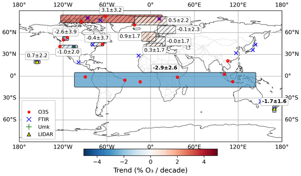
To visualize the spatial distribution of ozone recovery, we display global maps of trend estimates for all the partial columns defined above. Figures 20–22 and S2 show trends for the original sPCs, and Figs. 23, S3–S5 show trends for the alternative aPCs. The maps only display trends derived from BASIC-merged regional groups and not individual instruments' trends. This choice follows the methodology in order to maximize statistical significance and minimize trends uncertainty. However, it results in gaps in small geographical coverage – like in South America, Southern Africa, and Siberia – where the NDACC network density is insufficient to form groups.

In UpS (Fig. 20), trends are generally positive across the globe. We estimate robust recovery of +0.6 ± 0.7 % per decade in the Mid-Latitudes, +1.2 ± 0.8 % per decade in Central Europe, and +1.5 ± 0.9 % per decade in Lauder. In the alternative aUpS (20–1 hPa equivalent to 30–40 km, Fig. S3), the amplitude of these trends decreases, and they are non-significant for most regions (e.g., Mid-Latitudes +0.5 ± 0.6 % per decade; Central Europe +0.0 ± 0.6 % per decade). Scandinavia has a negative trend (−1.2 ± 2.1 % per decade). North Canada shows opposite trends in aUpS (positive, 1.4 ± 2.5 % per decade) than in UpS (negative, −3.0 ± 2.4 % per decade), underlying the limitations of BASIC for sparse datasets. Because of the polar night, the FTIR (only instrument in the group north Canada in UpS and aUpS) cannot measure during winter. The more important daily cycle (10 % near 50 km, according to Schranz et al., 2018) and the sensibility to NO_X (importance if the choice of proxies) suggests that our analysis here is not reliable.

In MS (25–30 km, Fig. 21), trends are negative and significant near the equator. The European continent, however, displays a mixture of negative non-significant trends: Central Europe group (+0.0 ± 0.9 % per decade), North Europe ($-\mathrm{1.2}\pm \mathrm{1.6}$ % per decade), South Europe (+0.2 ± 0.9 % per decade), and Svalbard/Greenland (−0.1 ± 2.6 % per decade). This points towards an underlying trend uncertainty in Europe, although it contains the densest networks of ground-based instruments. Strong significant negative trends are observed in the Equator and South Atlantic groups, as well as in Hawaii and the West US (−1.3 ± 1.1 % per decade). South Canada and North Canada show positive non-significant trends. These results generally agree more with the 25 km trend maps in Fig. 7 from Sofieva et al. (2026) than with the 30 km maps, consistent with negative trends in the lower part of the layer and a transition from positive to negative near 30 km altitude. In aMS (20–25 km, Fig. S4), trends are generally negative and non-significant, with few exceptions like Central Europe (−1.7 ± 1.2 % per decade), again consistent with the 25 km maps from Sofieva et al. (2026), which also reports from negative non-significant trends in the mid latitudes to weakly non-significant trends at 45° north and south. The East Coast US group shows a large decline, coherent with the strong depletion seen in the SCIAMACHY-OMPS 20 km maps (Sofieva et al., 2026).

In LS (15–25 km, Fig. 22), trends are mostly negative and non-significant, with even a significant negative trend at Lauder (already discussed in Sect. 4.2). Positive (non-significant) signals are seen in Hawaii (+0.7 ± 2.2 % per decade). The European trends are generally slightly positive, non-significant. This widespread negative trend is consistent with satellite measurements at 20 km (middle of LS) reported by Sofieva et al. (2026). In UTLS (10–20 km, Fig. 23), we find no significant negative trends in the Equator (−2.0 ± 3.1 % per decade) or Europe (0.2±3.0 % per decade). However, an exception appears over North America: the group East Coast US (+7.2 ± 3.6 % per decade) show significant positive trends. This contradicts the negative trends from satellite maps at 20 km. However, the UTLS partial column has a large vertical range (approx. 10–20 km), which includes part of the upper troposphere. From TOAR-II analyses (Van Malderen et al., 2025b) confirmed by Thompson et al. (2025), we expect positive tropospheric trends in these regions, so our UTLS result likely reflects an aggregation of two opposite evolutions: a positive trend in the upper troposphere masking the negative trend in the lower stratosphere. The OCTAV-UTLS findings (Millàn et al., 2025) underline the idea that the trends in pressure coordinates often combine signals from the troposphere and from the stratosphere, resulting in masking of the underlying trends.

Finally, trends in the standard troposphere (Fig. S2) are generally non-significant. An exception is the North Canada group, in aTROPO (Fig. S5), we find a positive significant trend (5.6 ± 3.2 % per decade), underlining the unreliability of our trends there.

5 Conclusions

In this study, we use the BAyeSian Integrated and Consolidated (BASIC) merging method to build regional composites of ground-based ozone partial columns for the 2000–2024 period and compare its performance with the conventional weighted mean (WM). BASIC is more robust in handling the heterogeneity of ground-based networks, such as in the Central Europe LS case study, where BASIC's uncertainty dynamically adapts to the data consensus level. Using a Gaussian-mixture likelihood and PCA uncertainties for outlier detection, BASIC produces adaptive posterior uncertainties that can increase monthly uncertainties when the instrumental consensus is poor, unlike the WM which does not adapt. While standard rejection techniques can easily remove obvious outliers, BASIC can also handle ambiguous values. Finally, despite larger composite uncertainties than the WM method, the trends uncertainties derived are smaller or comparable to those of the WM method, with an average reduction of 9.4 % in the BASIC trend uncertainty compared to WM's for the 3 selected regions. For the three groups of Lauder, Hawaii and Central Europe, the Upper Stratosphere generally shows positive trends, significant in Europe and Lauder. In contrast, the Middle and Lower Stratosphere commonly show negative or mixed signals. In some cases, the combination of BASIC and Partial Columns definition is able to identify significance in trends when the trends derived for individual instrument time series are not significant. In other cases, significance results mainly from the noise reduction associated with the partial column definition. For example, both BASIC and the WM estimated a significant negative trend in LS at Lauder, whereas satellite profile trends are not conclusive. In the tropics, Mauna Loa shows a transition from positive UpS to negative MS ozone trends, with an inversion above 10 hPa. However, the UTLS signal remains sensitive to the inclusion of the sparse FTIR dataset, the positive signal in TROPO and the choice of dynamical proxies.

Global maps generally support positive UpS trends over most regions and show predominantly negative MS trends, while LS trends are more regionally mixed and mostly non-significant. However, we find that composite trends in the UTLS over North America are likely subject to a masking effect, whereby upper-tropospheric positive trends may mask negative lower-stratospheric trends. Our ground-based composite global maps compare well with the satellite-composite global maps, although some limitations apply: the ground-based geographical coverage is uneven (with major gaps in South America, Southern Africa, and Siberia), and winter data gaps at high latitudes due to polar nights inflate trend uncertainties. Overall, BASIC is a robust method to merge ground-based partial-column datasets for regional ozone trend detection, providing a ground-based reference for global satellite assessments. However, BASIC provides limited added value when merging less than 3 instruments. This method is best suited to data-rich regions and cannot be used as an alternative to global coverage in regions where ground-based networks are absent. Looking forward, this work highlights the potential of BASIC merging as a standard for heterogeneous ground networks. Ground-based composites could then be compared to satellite-based composites. Future studies should focus on refining the trend estimation techniques, for instance by applying Dynamical Linear Modeling (DLM). Additionally, simulation studies that account for inter-instrument covariance would help to assess the representativeness of BASIC and WM composites. Further studies will investigate the contribution of partial column trends to the total ozone column trends of merged composites.