Constraining the atmospheric hydrogen oxidation and soil sink seasonal cycles using HFC-152a

As the hydrogen (H₂) economy expands, there is growing interest in understanding the atmospheric lifetime of H₂, which affects its impact on atmospheric chemistry and climate. While some global H₂ is destroyed via reaction with the hydroxyl radical (OH), most is lost to microbial activity in soils. However, the sources and sinks of H₂ are still uncertain on global and local scales. This study focuses on how monthly resolved observations of HFC-152a can help to constrain the seasonal OH cycle and the H₂ budget, particularly the seasonal range and phase of H₂ oxidation and soil loss. Seasonal observations of HFC-152a are used to constrain OH through a Bayesian inversion in a three-box model comprising the Northern, Tropics, and Southern regions over 2010–2022. In the North, a seasonal range of the soil sink of 18–21±8 Tg yr⁻¹ is found, peaking in July–August, while the OH loss seasonal range is 8±1 Tg yr⁻¹, peaking in July. The South has much less land and so displays a smaller soil sink seasonal range of 2–3±2.5 Tg yr⁻¹, peaking in January–March. The OH loss in the South has a seasonal range of 7±1 Tg yr⁻¹, peaking in January. The OH and soil sink loss in the Tropics is more consistent across all months, but with larger uncertainty. The results presented here will be a useful comparison for H₂ cycles in fully integrated chemistry climate models.

1 Introduction

There has been a growing interest in using hydrogen (H₂) as an alternative to fossil fuel (Hydrogen Council, 2020; IEA, 2023). H₂ itself is not a greenhouse gas; however, its main atmospheric sink is through reaction with the hydroxyl radical (OH), which in turn affects three major greenhouse gases: methane, tropospheric ozone, and stratospheric water vapor. Therefore, H₂ is an indirect greenhouse gas, with a net 100-year global warming potential (GWP) of around 8–12 (6–16 when including uncertainties) (Bertagni et al., 2022; Chen et al., 2024; Derwent, 2023; Ouyang et al., 2025; Warwick et al., 2023). As shown in the above studies, the rate of loss of hydrogen to soil is both large and highly uncertain and therefore dominates the uncertainty in this important GWP. With future emissions likely to increase as the H₂ economy increases, it is important to better understand the sinks of H₂.

The primary source of H₂ in the atmosphere is oxidation of methane and volatile organic compounds (VOCs) such as isoprene into formaldehyde (CH₂O), which then photolyzes to form H₂. H₂ can also be produced from combustion in auto engines. Overall, global anthropogenic emissions have likely been decreasing due to better air quality controls (Paulot et al., 2021). Biomass burning is another major source of H₂ emission (Crutzen et al., 1979), with large events coinciding with El Niño (Duncan et al., 2003). Hydrogen is leakage-prone from infrastructure. Therefore, if the H₂ economy were to increase in the future, this will also likely increase emissions and the atmospheric concentration of H₂ (Esquivel-Elizondo et al., 2023).

Atmospheric H₂ has a lifetime of ∼2 years resulting from two main sinks. The smaller of the two sinks is reaction with atmospheric OH, which is estimated to account for an approximate loss of 15–20 Tg yr⁻¹ (Ehhalt and Rohrer, 2013; Hauglustaine and Ehhalt, 2002; Novelli et al., 1999; Paulot et al., 2021; Sanderson et al., 2003; Yashiro et al., 2011). However, uncertainty remains on the impact of OH on H₂ and its subsequent impact on greenhouse gases due to model biases of OH, which typically overestimate the OH abundance (e.g. Yang et al., 2025).

The major sink of H₂ is through microbial driven near-surface soil uptake (Conrad et al., 1983), which predominantly occurs in the Northern Hemisphere (NH). This results in a greater concentration of H₂ in the tropics and Southern Hemisphere (SH) as seen from the National Oceanic and Atmospheric Administration (NOAA) global surface air sampling network (Novelli et al., 1999; Pétron et al., 2024). Soil uptake is also largely dependent on soil moisture and temperature, and therefore is expected to have a strong seasonality in the NH, likely peaking in the late summer/early autumn (Bertagni et al., 2021; Ehhalt and Rohrer, 2009; Reji et al., 2025; Yonemura et al., 1999). However, large uncertainties in the global and hemispherical loss due to soils remain, with published estimates ranging from ∼50–88 Tg yr⁻¹. For example, Rhee et al. (2006) used measurements of stable isotopic ratios of H₂ to infer a global soil sink of 88 Tg yr⁻¹, accounting for over 80 % of the total loss. Modelling studies that incorporate a moisture-based soil sink typically obtain lower values of ∼55 Tg yr⁻¹ (e.g. Brown et al., 2025a; Paulot et al., 2021; Pieterse et al., 2013) that peak between June–August depending on the model (Brown et al., 2025b). A recent model and observations synthesis of the H₂ budget arrives at a global soil sink of 50±18 Tg yr⁻¹ (Ouyang et al., 2025). Most current global climate models do not incorporate an interactive soil sink (e.g. Sand et al., 2023).

Methyl chloroform (CH₃CCl₃, MCF) has, previously, been used as the main reference gas to obtain the oxidative capacity of the atmosphere (Montzka et al., 2011; Naus et al., 2021; Patra et al., 2021; Prinn et al., 1992). When emissions of MCF were relatively well known, the retrieved uncertainty of mean tropospheric OH was fairly well constrained. But MCF is an ozone depleting substance and therefore production and consumption have been completely phased out since 2015 under the Montreal Protocol and its subsequent amendments. This resulted in near zero emissions and its global abundance dropped to very low levels. This increased uncertainty in the measured MCF values and derived OH, due for example to limits on instrument precision. A search for other viable candidates to constrain global mean OH is underway, with hydrofluorocarbons (HFCs) being a top contender (Liang et al., 2017; Thompson et al., 2024).

Here, the short-lived man-made gas HFC-152a is used to obtain information of the OH seasonality in a 3-box atmospheric model through an optimal estimation, similar to previous work using MCF (Bousquet et al., 2005). HFC-152a has been shown to be a viable alternative to MCF (Liang et al., 2017). The main loss pathway of HFC-152a, accounting for over 99 % of the loss, is through OH oxidation, with a short OH lifetime of 1.55 years (Burkholder et al., 2023; Ko et al., 2013). There is also a much smaller stratospheric sink with a lifetime of 44.3 years due to reaction with stratospheric OH, Cl, and O(¹D). Anthropogenic emissions are the only source of HFC-152a and are not well constrained (Simmonds et al., 2016; Western et al., 2025). Therefore, since OH is virtually the only sink, the uncertainties in emission limits the ability to retrieve accurate absolute OH values. The main uses of HFC-152a are as a propellant for industrial aerosols and as a blowing agent for extruded polystyrene foams (Liang and Rigby, 2023). Therefore, HFC-152a emissions are not expected to vary seasonally; thus, the short OH lifetime of HFC-152a allows for higher accuracy of the yearly range and phase of OH to be retrieved in this study, presented as seasonal anomalies (derived as a difference from the yearly mean). HFC-152a is also emitted mostly in the NH which results in a large North-South gradient (see Fig. 1). H₂ has observably different seasonality compared to HFC-152a in both the NH and SH. Therefore, the OH seasonal range and phase information obtained from HFC-152a can be used to help constrain the yearly ranges (maximum – minimum) and phase of the H₂ soil sink. This is highlighted in Fig. 1. At the Advanced Global Atmospheric Gases Experiment (AGAGE) (Prinn et al., 2025, 2018) site Mace Head (MHD, Ireland, 53.3° N) (Fig. 1a), HFC-152a exhibits a seasonal peak 1–2 months earlier than H₂, suggesting that the soil sink likely has a different phase than OH and CH₂O and is the dominant driver of the seasonality. At the AGAGE site Kennaook/Cape Grim (CGO, Australia, 40.7° S) (Fig. 1b), HFC-152a and H₂ are completely out of phase, suggesting that OH and CH₂O are the dominant drivers of H₂ seasonality. Absolute H₂ budget terms and overall lifetimes are not presented in this study because the absolute values of the retrieved OH are not constrained by our approach.

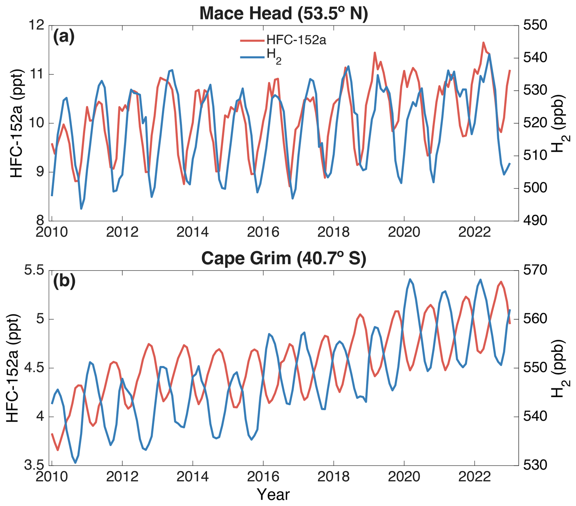
Figure 1 Comparison of HFC-152a and H₂ AGAGE times series at (a) Mace Head and (b) Cape Grim highlighting the different seasonal cycles and interhemispheric gradients.

The next section describes the forward model, observational and model data, and the inversion model used in the study. This is followed by results presenting initial forward model calculation and retrieval fits of HFC-152a and H₂. This is followed by retrieved OH and H₂ oxidation rates, presented as seasonal anomalies, averaged over 2010–2022 (2010 being the earliest start date that includes all observational sites). H₂ soil sink anomalies over the same period are then presented and discussed for each box. Conclusions are summarized in the last section.

2 Methods and Data

2.1 Box model

An equal mass three-box tropospheric model is constructed to act as the forward model of HFC-152a and H₂ mixing ratios. The box boundaries constitute the South (90–20° S), Tropics (20° S–20° N), and North (20–90° N) regions of assumed equal mass. Transport between the boxes is based on diffusive transport terms from (Cunnold et al., 1994), with modifications to account for the different box boundaries used in that study (0–30, 30–60, 60–90° N/S) by averaging the closest coincident terms. The values are then adjusted to ensure a realistic North-South gradient constrained by observations of the long-lived tracer, SF₆, from AGAGE. No short-lived species are explicitly calculated. Therefore, the forward model uses prior OH values and HFC-152a emissions to calculate HFC-152a, and uses prior OH values, H₂ emissions, CH₂O photolysis, and H₂ soil sink values to calculate H₂. The box model steps daily in time, and gas phase oxidation of HFC-152a and H₂ are calculated using an ERA5 monthly temperature time series over 2010–2022, averaged from the surface up to 200 hPa for each box (Hersbach et al., 2020). Transport and time series average temperature terms used in the box model are shown in Table S1 in Supplement. The Arrhenius equations used for the HFC-152a and H₂ oxidation reactions are from Burkholder et al. (2019) and are also shown in the Supplement.

2.2 Observations and forward model parameters

HFC-152a is used in the retrieval to optimize the monthly resolved OH concentration of each box over 2010–2022. HFC-152a has a very short OH lifetime of 1.5–1.6 years (Ko et al., 2013; Simmonds et al., 2016), allowing for the OH seasonal cycle to be derived from the measurements. It has been shown to be suitable for retrieving global average OH (Liang et al., 2017; Thompson et al., 2024). Monthly means of HFC-152a are derived from dry air mole fraction measurements at three AGAGE background sites (Prinn et al., 2025). The three representative sites used for each box in our model are: South box, Kennaook/Cape Grim (CGO, Australia, 40.7° S); Tropics box, Cape Matatula (SMO, American Samoa, 14° S); North box, Mace Head (MHD, Ireland, 53.3° N). Figure 1 shows a steep gradient in HFC-152a volume mixing ratio between the NH and the SH. Therefore, our choice of SMO for the Tropics box will likely be an underestimation of the tropical average. Indeed, a second Tropical location at Ragged Point (RPB, Barbados, 13.2° N) has higher mole fractions than SMO (not shown). However, this site was not used as it has more frequent intrusions of extra-tropical air. Instead, to account for the underestimation, a 20 % increase offset has been applied to the SMO data. H₂ observations used here come from AGAGE in situ measurements at CGO and MHD for the South and North boxes respectively and NOAA weekly flask measurements averaged over three stations: Ascension Island (United Kingdom, 8° S), Cape Matatula (American Samoa, 14° S), and Mahe Island (Seychelles, 4.6° S) (Pétron et al., 2024, 2025). Both AGAGE and NOAA datasets are on the MPI-2009 calibration scale. A comparison of the two AGAGE stations that make H₂ measurements (MHD and CGO) with a zonally and temporally resolved background air H₂ distribution based on the NOAA flask data is shown in Fig. S1 in the Supplement. In the South boxes, the two datasets are in excellent agreement. In the North box, there is a large spread in the range of NOAA values, but there is good agreement of the averages of the two datasets. This improves confidence that the single AGAGE station within each box gives a good representation of the entire box average. Even so, the large north-south gradient in the North box raises the question of whether the same agreement would hold for retrieval of the soil sink. To test this, the retrieval technique outlined in Sect. 2.3 was replicated using GFDL model data for OH, CH₂O, and Mace Head H₂ surface mixing ratios from Sand et al. (2023) with good agreement between actual model soil sink values and retrieved soil sink values (not shown). This gives further confidence that Mace Head is a good representation of the North box average. For the Tropics box, the average H₂ time series of the three NOAA stations listed above is also shown. Also, see Fig. S1 for the locations of the AGAGE stations and NOAA sites used in this study.

Emissions estimates for HFC-152a are taken from the Emission Database for Global Atmospheric Research (EDGAR: version EDGAR_2025_GHG) yearly emissions gridded dataset (Crippa et al., 2025). The data are supplied as annual grid map emissions, and it is assumed that the HFC-152a emissions do not vary over the course of a year in this study. There are differences between EDGAR emissions of HFC-152a and other emissions datasets (e.g. Western et al., 2025), and recent inversions (e.g. Thompson et al., 2024). Thus, the uncertainty in these emissions is reflected in the prior uncertainty value chosen for HFC-152a emissions of 15 % as described below.

Prior information for the seasonal amplitude of OH is taken from Spivakovsky et al. (2000) and scaled to match a global tropospheric OH concentration of 1×10⁶ molecules cm⁻³, in line with previous literature indicating a global tropospheric oxidative capacity between 0.9–1.0×10⁶ molecules cm⁻³ (Lawrence et al., 2001). However, it is important to note that some studies suggest a global abundance of OH as high as 1.13×10⁶ molecules cm⁻³ (Liang et al., 2017). As the HFC-152a emissions are not well constrained, the choice of OH prior concentration will influence the optimized OH values, but much less so the amplitude of the OH seasonal cycle in the North and South boxes, where HFC-152a has large seasonal cycles. This was confirmed by comparing optimized seasonal ranges of OH using three prior OH global mean values of 0.9×10⁶ molecules cm⁻³, 1.0×10⁶ molecules cm⁻³, and 1.1×10⁶ molecules cm⁻³, which shows virtually no sensitivity to the prescribed OH global mean value in the North and South boxes (see Fig. S2).

H₂ direct emissions data include biomass burning, anthropogenic, and nitrogen fixation emissions. Anthropogenic emissions of H₂ use H₂ to carbon monoxide (CO) emission factors (see Ehhalt and Rohrer, 2009; Paulot et al., 2021). These emissions factors are used to estimate H₂ emissions from different anthropogenic sources of CO from the current CMIP7 emissions dataset (these include inputs for residential, commercial, transportation, and shipping sources (Feng et al., 2020; Hoesly et al., 2025) for the 2010–2022 study period. Biomass burning emissions of H₂ from CMIP7 are directly available (van Marle et al., 2017; van Marle and Werf, 2025), so no conversion factor is needed. Anthropogenic emissions of CO, and therefore H₂, have likely been declining since 1990 due to stricter regulations of combustion emissions by vehicles (catalytic converter) and industrial processes (e.g. Ouyang et al., 2025). However, not all emissions of H₂ are contiguous with CO (Paulot et al., 2025), and therefore large uncertainty in emissions, and emission sources remain. Emissions from nitrogen fixation are also included in the model, totaling 9 Tg yr⁻¹ globally following Paulot et al. (2021). Global and individual box emissions of H₂ used in the forward model are shown in Fig. 2. The other major source of H₂ in the atmosphere is chemical production through a two-step process beginning with the oxidation of methane and VOCs to CH₂O, which then photolyzes into H₂. H₂ chemical production values are derived using two methods: (1) Using the specified dynamics version of the Whole Atmosphere Chemistry Climate Model (WACCM6) (Gettelman et al., 2019) photolysis rates of CH₂O from 975 to 200 hPa for the Tropics box and up to 300 hPa for the North and South boxes. These pressure values are chosen to ensure that only free tropospheric values are used while still maintaining over 90 % of column integrated loss (e.g. Liang et al., 2017). To account for any potential biases in the WACCM CH₂O, a scaling factor representing the difference between WACCM and the Tropospheric Ozone and its Precursors (TROPESS) CH₂O reanalysis seasonal amplitude was applied (Miyazaki et al., 2020). (2) Using the pseudo-linear OH-CH₂O relationship as described in Wolfe et al. (2019) to obtain H₂ chemical production rates from optimized OH:

$$\begin{array}{}\text{(1)}& \begin{array}{rl}{j}_{{\mathrm{CH}}_{\mathrm{2}}\mathrm{Ob}}& \left[{\mathrm{CH}}_{\mathrm{2}}\mathrm{O}\right]\\ & =j_{{\mathrm{CH}}_{\mathrm{2}}\mathrm{Ob}}{\displaystyle \frac{\mathit{\alpha }{k}_{\mathrm{OH}}^{\prime }\left[\mathrm{OH}\right]+P_{\mathrm{0}}}{j_{{\mathrm{CH}}_{\mathrm{2}}\mathrm{Oa}}+j_{{\mathrm{CH}}_{\mathrm{2}}\mathrm{Ob}}+k_{{\mathrm{CH}}_{\mathrm{2}}\mathrm{O}+\mathrm{OH}}\left[\mathrm{OH}\right]}}\end{array}\end{array}$$

Where $\mathit{\alpha }{k}_{\mathrm{OH}}^{\prime }$ [OH] describes the production of CH₂O through hydrocarbon oxidation, P₀ represents production from non-OH sources. $j_{{\mathrm{CH}}_{\mathrm{2}}\mathrm{Oa}}$ and $j_{{\mathrm{CH}}_{\mathrm{2}}\mathrm{Ob}}$ are the CH₂O photolysis frequencies, and $k_{{\mathrm{CH}}_{\mathrm{2}}\mathrm{O}+\mathrm{OH}}$ is the CH₂O oxidation rate constant. Slope ($\mathit{\alpha }{k}_{\mathrm{OH}}^{\prime }$ [OH]) and intercept (P₀) terms for each box are derived from TROPESS OH and CH₂O concentrations and from WACCM photolysis frequencies averaged over the same regions as method 1 and are shown in Fig. S3. The pseudo-linear relationship stems from the photolysis loss of CH₂O being greater than the production coming from oxidation of long-lived hydrocarbons, such as CH₄. However, this is likely not always the case in all regions and therefore should be treated as an approximation only, especially in the Tropics box as can be seen by the limited linear fit in Fig. S3. A constant prior H₂ soil sink was used in each box for the entire period to approximately close the H₂ budget.

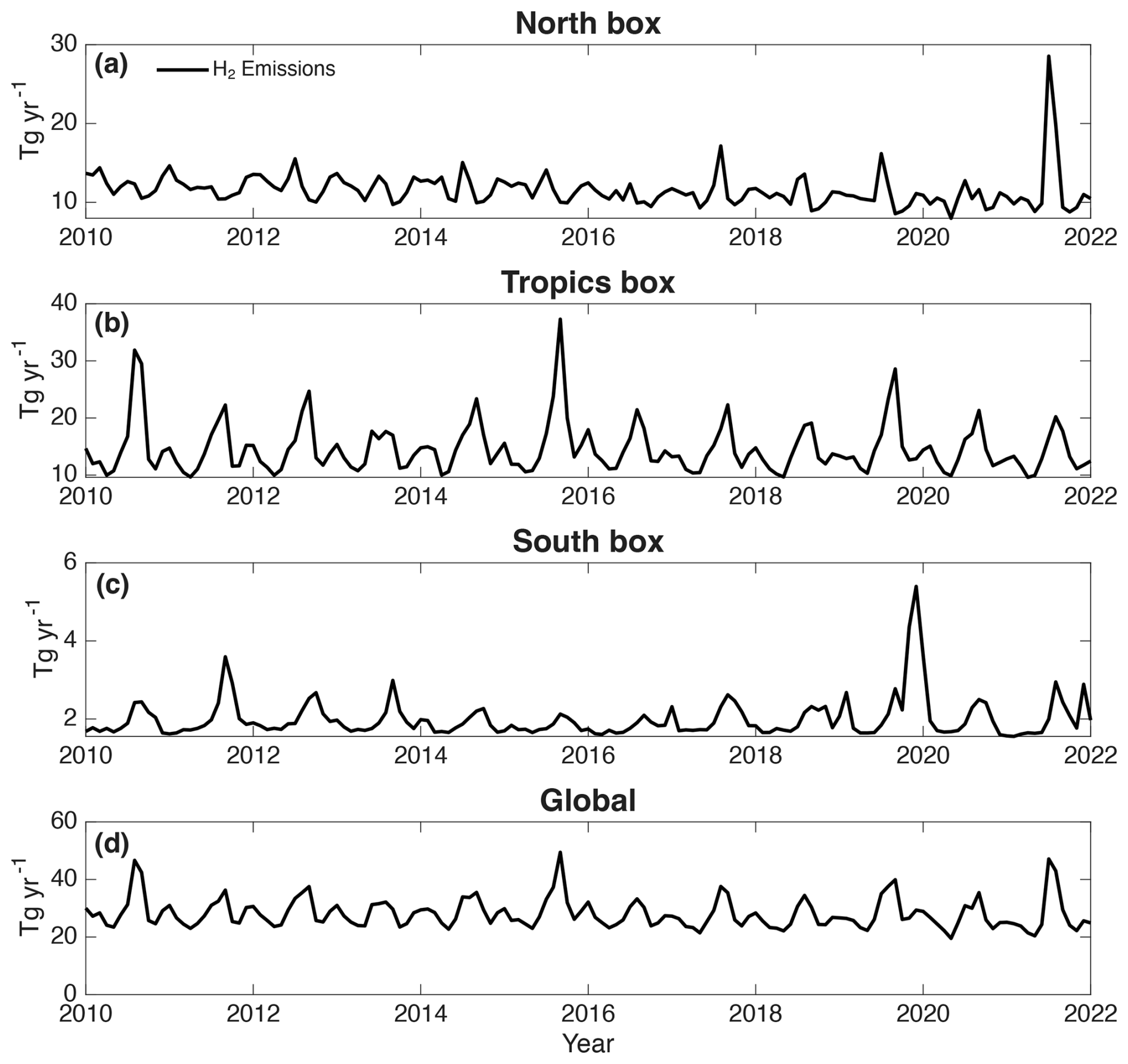
Figure 2 2010–2022 monthly prior emissions of H₂ used in the prior forward model calculation for the (a) North box, (b) Tropics box, (c) South box, and (d) globally.

2.3 Inversion model

The inversion model used in this study is a Bayesian optimal estimator (Rodgers, 2000). The model optimizes monthly average time series of OH, the time series of yearly emissions for HFC-152a, as well as the monthly average time series of the H₂ soil sink, emissions, and chemical production rates. The retrieved state vector is obtained by solving the following equation iteratively,

$$\begin{array}{}\text{(2)}& \begin{array}{rl}{\mathit{x}}_{i+\mathrm{1}}& ={\mathit{x}}_{\mathrm{a}}+{\mathbf{S}}_{\mathrm{a}}{\mathbf{K}}_i^T{\left({\mathbf{K}}_i{\mathbf{S}}_{\mathrm{a}}{\mathbf{K}}_i^T+{\mathbf{S}}_{\mathrm{e}}\right)}^{-\mathrm{1}}\\ & \left(\mathit{y}-\mathit{F}\left({\mathit{x}}_i\right)+{\mathbf{K}}_i\left({\mathit{x}}_i-{\mathit{x}}_{\mathrm{a}}\right)\right)\end{array}\end{array}$$

Where, for iteration i+1, x_a is the prior state vector, S_a is the prior error covariance matrix, K_i is the Jacobian from the previous iteration, S_e is the observational error covariance matrix, y are the observations, F is the forward model and x_i is the state vector from the previous iteration. The retrieval is run until convergence, determined by minimizing the following form of the cost function from Eq. (5.33) in Rodgers (2000),

$$\begin{array}{}\text{(3)}& d_i^{\mathrm{2}}={\left(\mathit{F}\left({\mathit{x}}_{i+\mathrm{1}}\right)-\mathit{F}\left({\mathit{x}}_i\right)\right)}^T{\mathbf{S}}_{\mathit{\delta }y}^{-\mathrm{1}}\left(\mathit{F}\left({\mathit{x}}_{i+\mathrm{1}}\right)-\mathit{F}\left({\mathit{x}}_i\right)\right)\ll m\end{array}$$

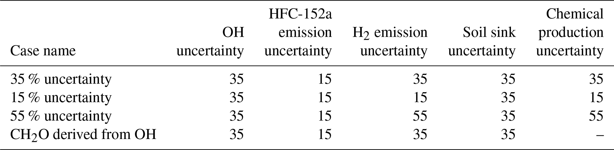
Where $S_{\mathit{\delta }y}^{-\mathrm{1}}$ is the inverse of covariance of the difference between the fit and the measurements, and m is the number of observational constraints. HFC-152a emissions uncertainty was set to 15 %, and OH uncertainty was set to 35 %. These values were obtained through an L-curve optimization to ensure the prior uncertainty values minimized retrieval uncertainties while avoiding overfitting (see Fig. S4). Considering that OH and CH₂O are strongly correlated, both methods in determining chemical production, as described in Sect. 2.2, are used in separate optimizations. Since there is a strong causal relationship between OH and CH₂O atmospheric concentrations, a zero-lag cross correlation between OH and CH₂O is implemented when model values of CH₂O photolysis rates are used directly. This ensures correct chemical production seasonality. When chemical production values are derived using Eq. (1), they are not optimized but calculated after each iteration in Eq. (2). Four retrievals are then performed to test the sensitivity of the soil sink amplitude on different setups: (1) using model values for chemical production with a prior uncertainty of 35 %, the same as OH, and H₂ emission uncertainty is also set to 35 %, (2) same as (1) but chemical production and H₂ emissions uncertainties set to 15 %, (3) Same as (1) but chemical production and H₂ emissions uncertainties set to 55 %, (4) using retrieved OH to derive chemical production following Eq. (1), and H₂ emission uncertainty is set to 35 %. The H₂ soil sink uncertainty is set to 35 % for all cases. This value was chosen as it is both the same as the OH uncertainty used and is a reasonable representation of the reported observation uncertainty (e.g. Brown et al., 2025b; Cowan et al., 2025). Case setups are summarized in Table 1. Note all uncertainties are expressed as normal distribution standard deviations. Prior emission values for HFC-152a are expected to be correlated in time for each box, therefore an exponential correlation function is used with a temporal correlation length of 5 years, similar to Thompson et al. (2024). A temporal correlation of 12 months was applied to H₂ emissions. This is much shorter than HFC-152a, as H₂ emissions are strongly dependent on seasonal biomass burning emissions. OH and CH₂O values are not expected to be correlated in time. H₂ soil sink temporal correlations are also not included due to large uncertainties in moisture thresholds on H₂ uptake (e.g. Reji et al., 2025). Introducing a 6-month temporal correlation produces only minor differences in retrieved soil sink anomalies (not shown). Marginal posterior standard deviation uncertainties are obtained from the square root of the diagonal terms of the posterior covariance matrix, S, which is defined as,

$$\begin{array}{}\text{(4)}& \mathbf{S}={\mathbf{S}}_{\mathrm{a}}-{\mathbf{S}}_{\mathrm{a}}{\mathbf{K}}^T{\left({\mathbf{S}}_{\mathrm{e}}+{\mathbf{KS}}_{\mathrm{a}}{\mathbf{K}}^T\right)}^{-\mathrm{1}}{\mathbf{KS}}_{\mathrm{a}}\end{array}$$

Table 1 Prior normal distribution standard deviation uncertainties, as percents of absolute values, used in all optimized configurations.

3 Result and discussion

3.1 Forward model and retrieved fits to observations

AGAGE and NOAA dry air mole fractions of HFC-152a and H₂ representing the “observed” means for the 3 model boxes are shown in Fig. 3. The modeled prior and retrieval posterior means are also shown. For HFC-152a, the major source of the seasonality in the North and South boxes is governed by loss to OH (also see Fig. 4), and therefore the North and South boxes have seasonality that is clearly out of phase and is well captured by the forward model. In the Tropics box, there is little observed seasonality and variability of HFC-152a (See Fig. 3b). The forward model does show repeated small amplitude double peaked seasonality that is due primarily to the double peak tropical OH prior mean and transport between boxes (See also, Fig. 4c). The differences in observed and modeled trends in HFC-152a are likely due to uncertainties in emissions estimates. Indeed, retrieved global emissions estimates for HFC-152a have a smaller yearly growth than the EDGAR emissions used in this study (see Fig. S5). This is in agreement with year-to-year changes from Thompson et al. (2024) and Western et al. (2025), with small differences in absolute values that are within retrieved uncertainties between the studies (not shown). Transport parameters between boxes used in the model can also influence individual box trends and are a source of uncertainty in this three-box model setup. The HFC-152a time series modelled using the retrieved emissions and OH values agree very well with the observations in all boxes with only slight discrepancies in sharp peaks in the observations, for example in 2018 in the North box (Fig. 3a). However, these differences are within the posterior standard deviation.

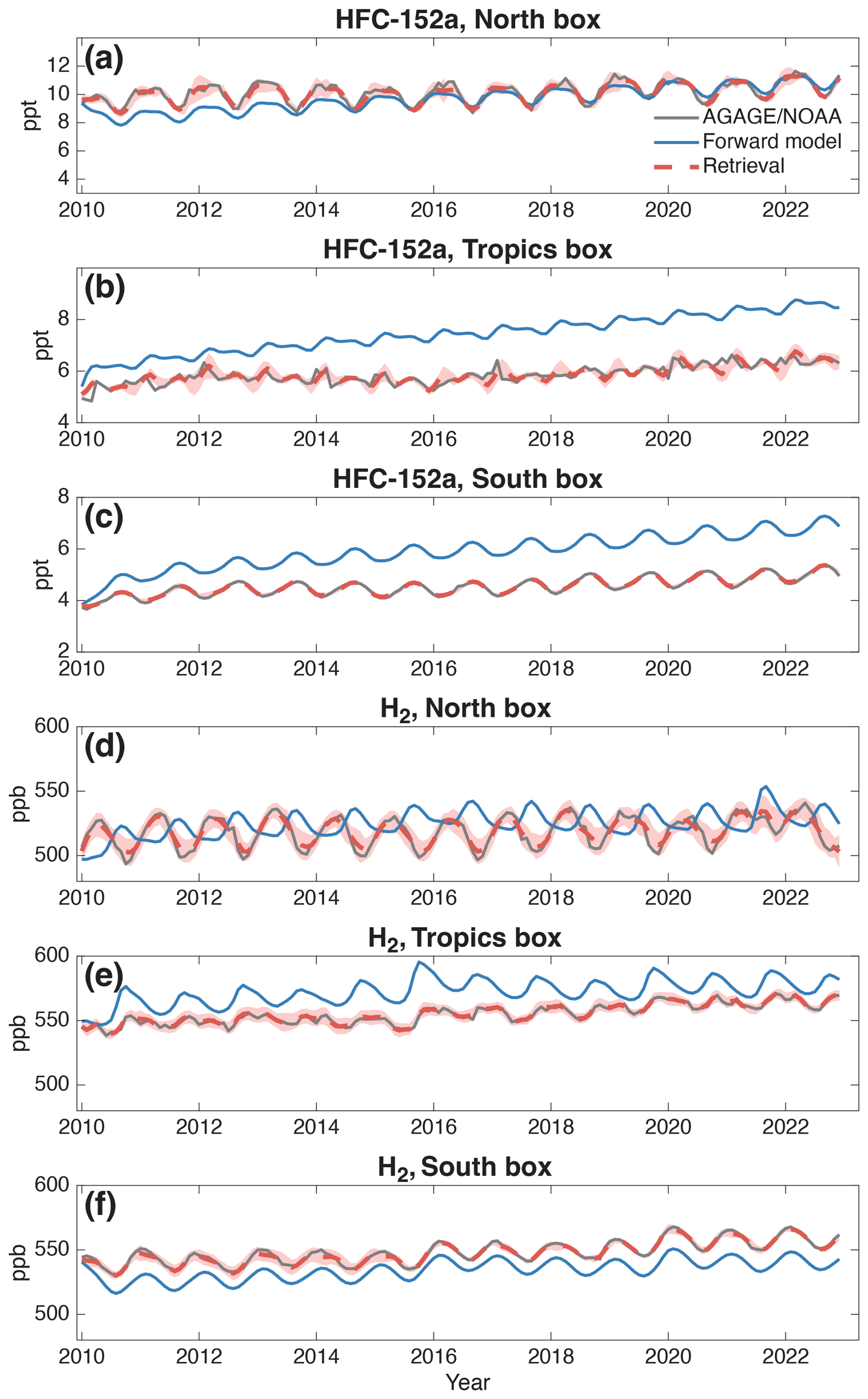
Figure 3 Comparison of the forward model (blue line), observations (gray line), and the retrieval fit (dashed red line) of HFC-152a and H₂ over 2010–2022. HFC-152a for the North box (20–90° N), Tropics box (20° S–20° N), and South box (20–90° S) are shown in panels (a), (b), and (c) respectively. Similarly, for H₂ in panels (d), (e), and (f). The retrieved fit is shown for the 35 % prior uncertainty case along with the posterior standard deviation (shaded region). For the North and South boxes, AGAGE data is used for both HFC-152a and H₂. For the Tropics box, AGAGE Cape Matatula data is used for HFC-152a, and NOAA data is used for H₂ (see Sect. 2).

In the North box, the forward model mole fractions of H₂ show very different seasonality compared to the observations (Fig. 3d). Since the initial forward model has a constant soil sink, it does not affect the seasonal cycle. Therefore, OH, chemical production, and H₂ emissions control the modeled seasonality, causing the large difference in phase and suggesting that the soil sink is likely the dominant driver of the observed seasonality (also see Fig. 1).

In the Tropics Box, the seasonal variability in the observations of H₂ is mostly controlled by biomass burning and chemical production, with larger changes occurring during years of larger biomass burning, such as in 2016 and 2020 (See Fig. S6). The large biomass burning emissions, in combination with an increasing trend in CH₂O results in observed step changes in H₂ in the Tropics and South Box (Pétron et al., 2024).

In contrast to the North box, in the South box, the forward model seasonality in the H₂ mole fraction is in good agreement with the observations (Fig. 3f). This is due to the seasonality in the SH being less dependent on the soil sink than in the North box. As the H₂ seasonality is completely out of phase to that of HFC-152a, OH and chemical production are likely the dominant driver of the observed seasonality in the South box. Similar to the Tropics box, the SH observations display a stepped increase in both 2016 and 2020 due to biomass burning that is captured well in the forward model. The initial agreement of the forward modelled mole fractions with observations in all boxes gives confidence that the prior values used here are a reasonable estimation of the competing sources and sinks in each box. The time series of H₂ modelled using the retrieved sources and sinks agree very well with the observations in all boxes.

3.2 Retrieval of OH

Monthly averaged prior mean and retrieved OH anomalies are shown for the North box (Fig. 4a) , Tropics box (Fig. 4b), South box (Fig. 4c), and globally (Fig. 4d), respectively for two cases (the 35 % prior uncertainty case and the CH₂O derived from OH case). The differences between retrieved OH anomalies are small between the two cases. Error bars show the posterior standard deviations for the 35 % uncertainty inversion case.

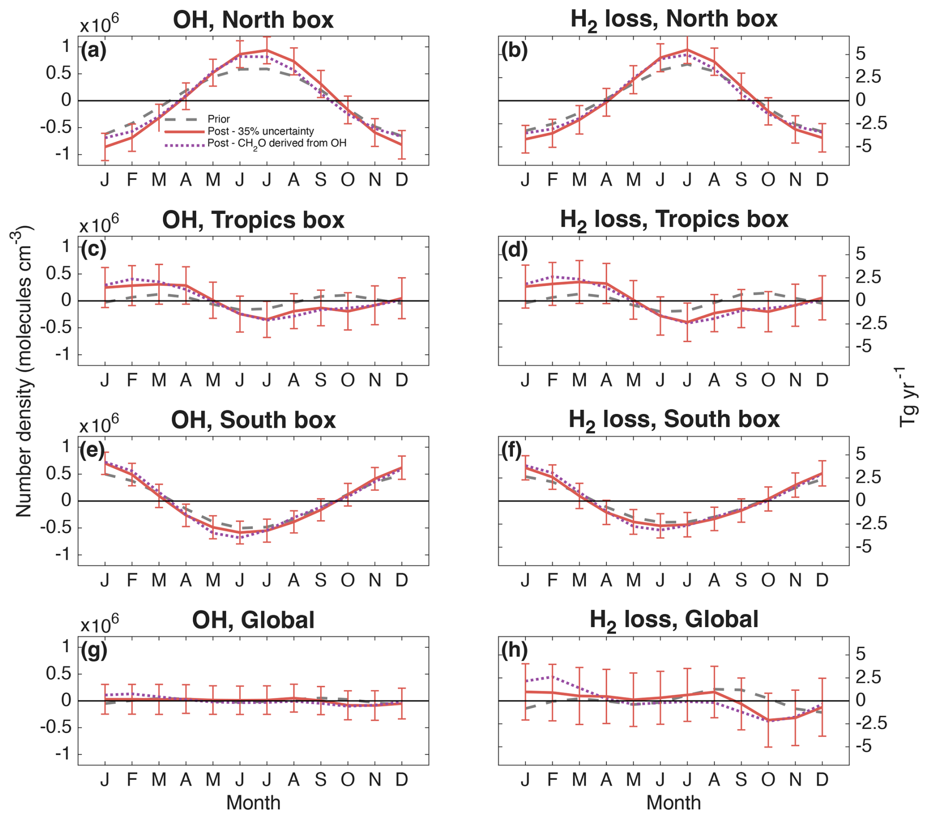
Figure 4 Monthly prior and retrieved mean anomalies for OH concentrations and H₂ oxidative loss rates for the (a, b) North box, (b, c) Tropics box, (d, e) South box, and (g, h) globally. The error bars show the retrieved posterior standard deviations calculated from the posterior covariance. The retrieved values are shown for the 35 % uncertainty and the CH₂O derived from OH cases. Monthly average values are taken from data over 2010–2022.

In the North box, the mean retrieved OH range is 16–17×10⁵ molecules cm⁻³, peaking in June–July, with a posterior standard deviation of 2.5×10⁵ molecules cm⁻³ (∼15 % of the range). The retrieved values have a higher and sharper peak than the prior mean with a difference in range of $\sim \mathrm{6.0}\times {\mathrm{10}}^{\mathrm{5}}$ molecules cm⁻³. The seasonal range and phase of values are in good agreement with a previous inversion for a 30–90° N box using MCF (Bousquet et al., 2005). This results in a peak H₂ oxidative loss occurring in June–July with a seasonal range of 8.0 Tg yr⁻¹ and a posterior standard deviation of 1 Tg yr⁻¹ (Fig. 4b).

In the Tropics (Fig. 3c and d), the retrieved OH seasonal range is much smaller, at $\sim \mathrm{0.5}\times {\mathrm{10}}^{\mathrm{5}}$, compared to the North box. The posterior standard deviation is $\sim \mathrm{0.25}\times {\mathrm{10}}^{\mathrm{5}}$ (∼50 % of the range) and a peak OH value is retrieved in February–March. However, as the seasonal signals of HFC-152a observations in the tropics are less consistent year-to-year compared to the North and South boxes, the Tropics box retrieval is more sensitive to changes in initial OH and transport conditions (see Figs. 3 and S2). This results in a yearly range in H₂ loss of 4 Tg yr⁻¹ with a posterior standard deviation of 2.5 Tg yr⁻¹.

The South box has a lower retrieved OH range compared to the North box, at 13×10⁵ molecules cm⁻³, peaking in December–January, with a posterior standard deviation of 2.0×10⁵ molecules cm⁻³ (∼15 % of the range). These lower values, along with the slightly lower temperatures in the South box result in a retrieved range of H₂ oxidative loss of 7 Tg yr⁻¹ and a retrieved uncertainty of 1 Tg yr⁻¹. Overall, the optimized global OH concentration and H₂ oxidative loss is consistent over the year (Fig. 4g).

3.3 Retrieval of the soil sink

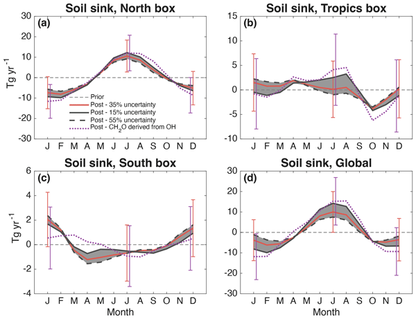
Figure 5 shows the soil sink retrieval for all inversion cases (see Sect. 2). Posterior standard deviation uncertainties are shown for the 35 % uncertainty and the CH₂O derived from OH cases as error bars. The range in the retrieval means for the 15 %, 35 %, and 55 % uncertainty cases is shown as the shaded area, which is less than half of the 1-standard deviation uncertainty for a single case. It is important to emphasize that the prior soil sink is constant over the course of a year. Therefore it has no impact on the seasonal anomaly that is retrieved and is hence a key finding of this paper. In the North box (Fig. 5a), the soil-sink seasonal cycle peaks in July and August with a seasonal range of 18–21 Tg yr⁻¹ and posterior standard deviation of 8 Tg yr⁻¹, and displays seasonality in agreement with current understanding of the moisture dependence of soil uptake in the NH (Bertagni et al., 2021). The minimum occurs in January–February. There is reasonable agreement between the two methods of deriving chemical production. When deriving CH₂O from OH values, the peak occurs slightly later and with a slightly larger range compared to when CH₂O is also optimized. The posterior standard deviations between the two cases are also similar. The range between all cases is primarily a result of the prior range of estimates on the CH₂O uncertainty, highlighting the importance of accurately modelling free tropospheric CH₂O for simulating the H₂ budget (see Fig. S7). In this study, even though our retrieved CH₂O is directly linked to our retrieval of OH, our prior values are derived from model and reanalysis estimates and are therefore a source of uncertainty. The results provide a basis for testing the fidelity of land models for the seasonal phase in uptake of H₂ by soil in northern latitudes.

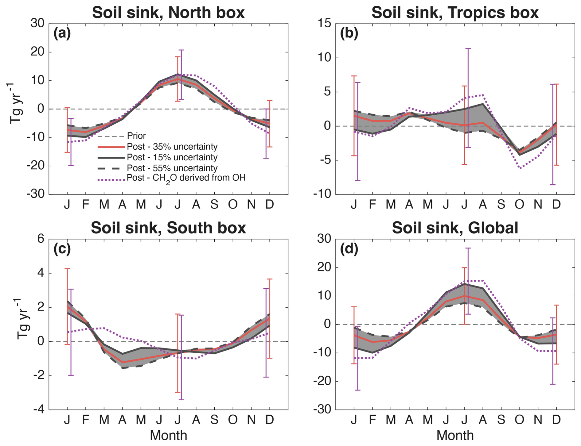
Figure 5 Monthly anomalies of the H₂ soil sink from the yearly mean for all cases in (a) the North box, (b) the Tropics box, (c) the South box, and (d) globally. The shaded region shows the range between the 15 %, 35 %, and 55 % uncertainty cases (see Table 1). The CH₂O derived from OH case (dotted line) is also shown. The error bars show the retrieved posterior standard deviation uncertainty for the 35 % uncertainty case and the CH₂O derived from OH case for select months of January, July, and December. The grey dashed line shows the prior estimate for the soil sink in each box. Results are averaged over the 2010–2022 time series.

In the Tropics box (Fig. 5b), the retrieved soil sink shows smaller seasonal range compared to the North box. The largest range is retrieved in the CH₂O derived from the OH case at 8 Tg yr⁻¹ with a posterior standard deviation of 8 Tg yr⁻¹, which peaks in July–August, similar to the North box. This is also the time of maximum variation between the three cases, which is partly driven by the time of maximum biomass burning that peaks in the Tropics box (see Fig. S8). The seasonal phase of the Tropics box soil sink agrees fairly well with the previous soil sink inversion by Bousquet et al. (2011). Although, it is important to note the significance is limited in this study as the retrieved posterior standard deviation is of similar magnitude to the range.

In the South box (Fig. 5c), the smallest soil sink range is retrieved at 2–3 Tg yr⁻¹ with a posterior standard deviation of 2.5 Tg yr⁻¹. The soil sink peaks in January–February and has a minimum in April for the 15 %, 35 %, and 55 % uncertainty cases and peaks in March and has a minimum in July for the CH₂O derived from OH. This is different than what was reported in some previous retrieval studies that show a peak loss in November (Bousquet et al., 2011; Xiao et al., 2007), but is in better agreement with others that show soil loss peaking in February (Rhee et al., 2006). However, the small range leads to limited significance outside of the posterior standard deviation. Other sources of retrieval differences could be the choice of the box northern boundary at 20° S. For example, Xiao et al. (2007) used a 4-box model with a boundary at 30° S. The small South box seasonal range is expected due to there being significantly less land compared to the North and Tropics boxes.

The global H₂ soil sink yearly mean range retrieved is 26 Tg yr⁻¹ for the CH₂O derived from OH case and between 13 and 23 Tg yr⁻¹ for the 15 %, 35 %, and 55 % uncertainty cases (Fig. 5d). All cases peak in July–August consistent with other observational and modelling studies (e.g. Bousquet et al., 2011; Brown et al., 2025b). The 35 % uncertainty and CH₂O derived from OH cases have a posterior standard deviation of 10 Tg yr⁻¹. The yearly average soil sink contributions from each box are retrieved as 43 %–46 %, 41 %–46 %, and 11 %–13% for the North box, Tropics box, and South box respectively over all cases. Additionally, the seasonal range of deposition velocities (cm s⁻¹) calculated using the retrieved soil sinks for each box are in reasonable agreement with current modelling estimates and observations at NH sites when considering the different latitudinal boundaries. For example, our North box range is ∼0.018–0.023 cm s⁻¹ over 20–90° N compared to ∼0.027 cm s⁻¹ over 30–90° N for the H₂-flux model simulations in Brown et al. (2025a).

The soil sinks yearly ranges and phases shown here are most consistent between the cases for the North and South boxes where the OH seasonal cycles retrieved from HFC-152a are most robust. Since the seasonal cycle of chemical production through CH₂O photolysis in this study is either strongly correlated to OH in the prior covariance or derived from retrieved OH using Eq. (1), and the seasonal cycle of emissions of H₂ are tied to biomass burning and anthropogenic seasonality, there is confidence in the retrieved phase of the soil sink. This is especially the case in the North box, South box, and globally (since the majority of the H₂ soil loss is occurring in the NH). The Tropics box retrieved OH is more sensitive to initial OH and transport conditions (Fig. S2) and observed HFC-152a in the Tropics box shows much larger year-to-year variability in the seasonal cycle (Fig. 3). Therefore, confidence in the Tropics box retrieved soil sink phase is lower than the North box and is reflected in the differences in phase between the cases (Fig. 5b). The amplitude of the retrieved seasonal cycle is, however, dependent on the prior values for chemical production and H₂ emissions and is the reason for large prior uncertainties used, which results in large posterior uncertainty. This is especially the case in the Tropics box due to larger chemical production and OH loss values compared to other boxes, and larger H₂ emissions compared to the South box. However, the retrieved chemical production and H₂ emission anomalies are consistent among cases for all boxes, with the largest differences between cases relative to the seasonal amplitude seen in the Tropics box chemical production (see Figs. S7 and S8). The H₂ soil sink retrieved posterior standard deviation is ∼20 % less compared to the prior, indicating that we have increased precision in the soil sink retrieval.

4 Conclusions

A three-box model inversion of OH concentration and the sources and sinks of H₂ is presented in this study, revealing seasonal changes in oxidative loss and soil uptake. The three-box model uses an equal mass tropospheric box model with the three boxes prescribed as: North (20–90° N), Tropics (20° S–20° N), and South (90–20° S).

The inversion uses a Bayesian optimal estimation of monthly resolved OH, the H₂ soil sink, H₂ chemical production through CH₂O photolysis, and H₂ emissions in the three boxes. Monthly information of HFC-152a and H₂ dry air mixing ratios from the Advanced Global Atmospheric Gases Experiment (AGAGE) and the National Oceanic and the Atmospheric Administration (NOAA) global surface air sampling network are used to constrain the OH signal. This information is then used to infer the seasonal anomaly of H₂ oxidation in each box. Anomalies only, rather than absolute values, are analyzed because HFC-152a emissions are not well constrained, which limits the ability to retrieve accurate absolute OH values, which then in turn affects the absolute soil sink retrieval. The retrieval of the seasonal range and phase in the North and South boxes is however relatively independent of prior OH mean values and transport terms used between the boxes for the scenarios tested here. Due to the large correlations between H₂ sources and sinks, particularly OH loss and chemical production, and the uncertainties in H₂ emissions, three retrievals are conducted spanning a range of prior uncertainties for CH₂O photolysis and H₂ emissions of 15 %, 35 %, and 55 %. In these cases, prior OH uncertainty is cross correlated with chemical production obtained from WACCM model simulations and TROPESS reanalysis. An additional case where H₂ chemical production is derived from retrieved OH data is performed using a pseudo-linear relationship between OH and CH₂O.

Between the two methods of retrieving H₂ chemical production, the retrieved OH is nearly identical due to the inclusion of HFC-152a data. The largest seasonal range of H₂ oxidative loss is retrieved in the North box at 8 Tg yr⁻¹, compared to the South box of 7 Tg yr⁻¹. The retrieved posterior standard deviation is 1 Tg yr⁻¹ for both the North and South boxes. The oxidative loss peaks in July in the North box and January in the South box.

The North box retrieved soil sink has a range of 18–21 Tg yr⁻¹ between the 4 cases that peaks in July–August with a posterior standard deviation of 8 Tg yr⁻¹, while the South box has a much lower soil sink range of 2–3 Tg yr⁻¹ peaking in January–March between the four cases with a posterior standard deviation of 2.5 Tg yr⁻¹. The OH and soil sink loss in the Tropics region is more consistent throughout the year but has larger uncertainty in both the phase and amplitude of the soil sink. Globally, there is consistency in the phase of the soil sink which peaks in July–August, however, there are larger differences between cases in the range compared to the North box of between 13–26 Tg yr⁻¹ with a posterior standard deviation of 10 Tg yr⁻¹.

Retrieving OH through HFC-152a seasonality with inferred or correlated chemical production of H₂ gives confidence in the North and South box soil sink seasonal phase retrieved here. However, uncertainty in the seasonal range of the soil sink, reflected in the large posterior standard deviations is dependent on prior uncertainty in CH₂O and H₂ emissions. Therefore, further constraining the soil sink will require reducing these uncertainties. Nonetheless, the results presented here provide a useful tool for fully coupled land chemistry climate models to verify seasonal soil uptake when incorporating an interactive hydrogen scheme.