Changes in global atmospheric oxidant chemistry from land cover conversion

Human activities have profoundly altered natural vegetation, primarily by converting pristine natural land to agriculture and grazing. Land cover change (LCC) influences the Earth system through modifications of surface albedo, roughness length, evapotranspiration, and atmospheric composition. This work investigates how LCC-driven changes in biogenic volatile organic compound (BVOC) fluxes, anthropogenic surface emissions, natural soil NO emissions, and O₃ deposition fluxes affect atmospheric chemistry. The chemistry–climate model EMAC was used to compare: (1) present-day land cover, which includes areas deforested for crops and grazing, with the potential natural vegetation (PNV) cover simulated by the model, and (2) an extreme reforestation scenario where grazing land is restored to natural vegetation. Our results show that the expansion of agricultural land reduces global BVOC emissions, leading to larger annual average surface OH concentrations (+5.7 %) and lower CO mixing ratios (−6.2 %), despite increased CO from agricultural burning. Meanwhile, NO_x mixing ratios increase (+7.8 %) due to enhanced anthropogenic and natural soil sources. While regional ozone responses vary, global ozone production sensitivity shifts from a NO_x- to a VOC-sensitive regime. These changes influence radiative forcing with reductions in tropospheric O₃ and CH₄ lifetimes exerting a combined radiative effect of −60 mW m⁻² (cooling), partially offsetting the warming from reduced BVOC-driven aerosol formation. Reforestation of grazing areas reverses these trends to some extent, though with a weaker response.

1 Introduction

Human activities have led to substantial transformations in Earth’s natural vegetation, with forests particularly impacted due to extensive conversion to agricultural land. This large-scale land cover change (LCC) has significantly influenced the Earth system, affecting nearly half of the global land surface (Hurtt et al., 2011). As a central component of Earth’s biophysical and biogeochemical systems, the biosphere is markedly altered by LCC as it changes major biogeochemical cycles and modifies interactions with the atmosphere (Bonan, 2008). Forests, which store approximately 45 % of the world’s terrestrial carbon, act as a critical carbon sink, capturing and sequestering carbon that would otherwise remain in the atmosphere and contribute to global warming (Field, 2004; Pan et al., 2011). Additionally, forests play a key role in regulating the hydrological cycle through evapotranspiration, which influences atmospheric moisture levels, cloud formation, and precipitation patterns, ultimately impacting regional and global climate, including surface temperature (Betts et al., 2004; Vicente-Serrano et al., 2015; Swann et al., 2012). Land cover further modulates the planetary albedo; dense forest canopies can absorb up to 90 % of incoming solar radiation, thereby impacting surface reflectivity and playing a main role in the Earth’s surface energy balance (Gibbard et al., 2005).

The terrestrial biosphere is the primary source of biogenic volatile organic compounds (BVOCs), such as isoprene and various terpenes, which comprise nearly 90 % of total volatile organic compound (VOC) emissions into the atmosphere (Guenther et al., 1995). Biogenic VOCs are highly reactive, readily interacting with tropospheric oxidants to produce lower volatility oxidation products that can partition into the aerosol phase, contributing to the formation of biogenic secondary organic aerosols (bSOA) (Heald et al., 2008) and also participating in new particle formation in pristine regions (Curtius et al., 2024).

The reactivity of BVOCs has been shown to influence global atmospheric aerosol loading, with implications for cloud properties and radiative balance (Spracklen et al., 2011; Scott et al., 2014). Numerous modelling studies have investigated how LCC influences aerosol loading, highlighting significant atmospheric and climate impacts. In particular, deforestation has been shown to reduce the global atmospheric aerosol burden, resulting in a net radiative warming effect (Vella et al., 2025; Scott et al., 2018; Heald et al., 2008).

Biogenic VOC oxidation not only contributes to atmospheric aerosol formation but also plays a crucial role in determining the concentrations of key atmospheric oxidants, such as hydroxyl (OH) radicals, ozone (O₃), and nitrate (NO₃) radicals, thereby modulating the atmosphere's oxidative capacity (Atkinson, 2000; Atkinson and Arey, 2003). The predominant reaction pathway for BVOCs is with OH radicals, which are primarily formed through the photodissociation of ozone in the presence of water vapour (Levy, 1971). While BVOCs initially deplete OH radicals through oxidation, they also contribute to OH recycling through subsequent reactions and, therefore, maintain the oxidation capacity of the atmosphere (Lelieveld et al., 2008). This complex interaction, often termed OH reformation, is essential for sustaining the troposphere's self-cleaning ability in view of the high levels of reactive BVOCs emitted by vegetation. The recycling process involves the formation of peroxy radicals (RO₂), which react with nitrogen oxides (NO_x) to produce ozone (O₃) and other oxidised products. As a result, BVOCs modulate O₃ concentrations in the troposphere, which acts as both a pollutant and a greenhouse gas (Atkinson, 2000; Lelieveld et al., 2016). In addition to daytime oxidation by OH, BVOCs can also be oxidised by O₃, and NO₃ radicals during the night, further influencing their atmospheric lifetimes and the concentrations of other trace gases (Atkinson and Arey, 2003). Changes in BVOC emissions and, therefore, OH reactivity also influence the atmospheric lifetimes of methane (CH₄) and carbon monoxide (CO), as OH radicals are a primary sink of these gases (Lelieveld et al., 2016).

As forests are converted to agricultural or urban land, BVOC emissions decrease, changing the delicate balance of atmospheric chemical reactions and influencing global oxidant chemistry. Several studies (e.g. Keller et al., 1991; Unger, 2014; Tripathi et al., 2025) have suggested that lower BVOC emissions from deforestation lead to higher OH concentrations, thereby shortening the lifetimes of CH₄ and O₃ and influencing global radiative forcing. In contrast, increased BVOC emissions in future reforestation scenarios are found to have the opposite effect (Weber et al., 2024). At the same time, some studies suggest that the global atmospheric oxidising capacity, and thus methane lifetime, remains largely unaffected by LCC (Heald and Spracklen, 2015; Ganzeveld et al., 2010; Ashworth et al., 2012). In addition to changes in BVOC emissions, land cover practices involve direct emissions in the atmosphere, for example, black carbon (BC) and carbon monoxide (CO) from agricultural waste burning and NO_x and NH₃ emissions from manure management (Denier van der Gon et al., 2023). LCC-driven NO_x emissions account for approximately 5 % of global emissions and play a key role in the HO_x cycle, significantly contributing to OH budgets alongside BVOCs (Denier van der Gon et al., 2023; Elshorbany et al., 2010).

In this work, we apply the chemistry–climate model EMAC coupled with the dynamic global vegetation model LPJ-GUESS to investigate the impacts on oxidant chemistry from changes in BVOC emissions and surface anthropogenic emissions following crop and grazing land expansion on potential natural vegetation (PNV). Potential natural vegetation refers to the type of vegetation that would naturally occur in a specific area under certain climate, soil, and environmental conditions without human influence. Land cover change is simulated through a deforestation routine in LPJ-GUESS (which simulates PNV), systematically clearing crop and grazing land areas based on 2015 land cover data. Additionally, we explore an extreme reforestation scenario where present-day grazing land is restored to natural vegetation. This work provides new insights into LCC-driven impacts on biogeochemical cycles by using state-of-the-art chemical representations in EMAC coupled with interactive vegetation calculations. This work provides comprehensive estimates of changes in atmospheric composition and non-aerosol radiative effects resulting from land cover change. For the first time, we present evidence that land cover change can affect the formation sensitivity of ozone, with important implications for both air quality and climate.

2 Model description and methods

2.1 The EMAC modelling system

The EMAC (ECHAM/MESSy Atmospheric Chemistry) model is a numerical chemistry and climate modelling system incorporating submodels that simulate tropospheric and middle atmospheric processes and their interactions with oceans, land surfaces, and human activities. It combines the ECHAM atmospheric general circulation model (GCM) (Roeckner et al., 2006) with the Modular Earth Submodel System (MESSy) framework (Jöckel et al., 2005), which structures physical–chemical processes and much of the model infrastructure into modular submodels. This design enables the further development of existing processes and the addition of new submodels to introduce new or alternative process representations.

Heterogeneous and gas phase chemistry are computed in the MECCA submodel (Sander et al., 2019), which employs the Mainz Isoprene Mechanism (MIM1) as the degradation chemical scheme (Pöschl et al., 2000; Jöckel et al., 2006). MIM1 includes over 100 gas phase species and more than 250 reactions. While the original MIM1 mechanism accounted for isoprene oxidation by OH and O₃, here we use the an extended version which additionally includes the oxidation of monoterpenes (treated as lumped species) by OH, O₃, NO₃, and O(¹D) (Tsimpidi et al., 2014). To investigate the production and loss pathways of tropospheric chemical reactions in this study, we used the kinetic chemistry tagging method of Gromov et al. (2010). This technique quantifies the turnover rates of key tracers (in this study: OH, HO₂, NO, NO₂, O₃, CH₄, and tropospheric O₃) within the MIM1 chemistry scheme in EMAC. It provides a comprehensive assessment of OH sources and sinks, enabling the evaluation of changes in the atmosphere's oxidation capacity. By decoupling diagnostic calculations from the primary chemistry scheme, the method achieves this level of detail with minimal additional computational overhead.

Dry deposition, sedimentation, and wet deposition are simulated by the submodels DDEP, SEDI (both Kerkweg et al., 2006), and SCAV (Tost et al., 2006a), respectively. Aerosols are treated using the submodel GMXe (Pringle et al., 2010), in which aerosol are represented by seven interactive lognormal modes that span the typical size range of aerosol species. These modes are further categorised into four hydrophilic (nucleation, Aitken, accumulation, and coarse) and three hydrophobic (Aitken, accumulation, and coarse) aerosol modes. The representation of all aerosols assumes spherical particles. The properties of aerosols in each mode are fully determined by the total mass (internal mixture of contributing species), density, number concentration, median radius, and width of the lognormal distribution. After each simulation step, aerosols may transfer between modes due to size changes and shift from hydrophobic to hydrophilic modes depending on their composition. Organic aerosol species are additionally described by the Organic Aerosol Composition and Evolution (ORACLE) submodel (Tsimpidi et al., 2014, 2018), taking into account the partitioning between aerosols and the gas phase organics based on the volatility basis set (VBS) framework (Donahue et al., 2006).

Convective cloud processes are taken into account based on the approach proposed by Tost et al. (2006b), using the convection schemes from Tiedtke (1989) and Nordeng (1994). Convective cloud microphysics is solely based on temperature and moisture profiles, without accounting for the influence of aerosols on liquid droplet or ice formation processes. Large scale stratiform clouds are described by the CLOUD submodel, which in the applied configuration employs the original ECHAM5 cloud scheme without aerosol–cloud interactions.

LPJ-GUESS (Smith et al., 2001, 2014) is a dynamic global vegetation model that features an individual-based approach to modelling vegetation dynamics. These dynamics are simulated as the emergent outcome of plant growth and competition for light, space, and soil resources among woody plant individuals and a herbaceous understorey in each of a number (50 in this study) of replicate patches representing random samples of each simulated locality or grid cell. The simulated vegetation is classified into 12 plant functional types (PFTs) discriminated by growth form, phenology, photosynthetic pathway (C₃ or C₄), bioclimatic limits for establishment and survival, and (for woody PFTs) allometry and life history strategy. The LPJ-GUESS version used in this study (v4.0) currently provides information on potential natural vegetation (PNV) and it does not incorporate LCC. In this work, however, a custom deforestation routine was integrated to constrain the PNV using deforestation maps. The deforestation maps are imported from external files and contain values ranging from 0 to 1. A value of 1 indicates complete deforestation within the respective grid cell, while intermediate values (e.g. 0.5) represent partial deforestation. For instance, a value of 0.5 corresponds to the removal of 50 % of the tree PFTs in that grid cell. The routine eliminates the tree PFTs after every simulated year and inhibits trees from establishing in the specified areas. This implementation allows us to constrain the vegetation cover and address the research questions presented in this work. However, the latest version of LPJ-GUESS (v4.1) features a more advanced land cover scheme, which will be incorporated into our current LPJ-GUESS version in future developments.

2.2 EMAC–LPJ-GUESS configuration

In this work, we use the standard EMAC–LPJ-GUESS (Forrest et al., 2020; Vella et al., 2023a) coupled configuration, where the vegetation in LPJ-GUESS is entirely determined by the EMAC atmospheric state, soil type, N deposition, and CO₂ fluxes, but there is no feedback from the vegetation to climate variables except for terrestrial BVOC emissions and O₃ dry deposition fluxes. The roughness length and albedo are kept at constant background values. Albedo is derived from satellite climatologies, while the roughness length is based on subgrid scale orography and satellite-derived vegetation climatology. Vegetation changes do not feed back to the hydrological cycle. We use the native bucket model in ECHAM5, which employs fixed climatological vegetation (Hagemann, 2002). In this setup, BVOCs are interactive tracers that can be oxidised to form secondary organic aerosols. This means that BVOCs can influence both the oxidant chemistry of the atmosphere and the aerosol load; however, this study focuses on the gaseous constituents and their respective changes.

After each simulation day, EMAC computes the average daily values of 2 m temperature, net downwards shortwave radiation, and total precipitation and passes these state variables to LPJ-GUESS. Vegetation information (leaf area index, foliar density, leaf area density distribution, and PFT fractional coverage) from LPJ-GUESS is then fed back to EMAC for the calculation of BVOC emissions. In this study, the BVOC fluxes in EMAC are calculated using the Model of Emissions of Gases and Aerosols from Nature (MEGAN) version 2.04 (Guenther et al., 2006).

MEGAN is based on the work of Guenther et al. (1993, 1995), where the BVOC emission flux is calculated as a function of PFT-specific emission factors and dimensionless activity factors. These activity factors consider sensitivities to the canopy environment, including parameters such as leaf area index (LAI), temperature, light, and leaf age. Notably, the current setup does not incorporate sensitivity to soil moisture. The parameterised canopy environment emission activity (PCEEA) algorithm is used rather than the alternative detailed canopy environment model that calculates light and temperature at each canopy depth. The PCEEA algorithm calculates the light sensitivity within the canopy as a function of the daily average above canopy photosynthetic photon flux density, the solar angle, and a non-dimensional factor describing the photosynthetic photon flux density transmission through the canopy.

This setup employs BVOC–aerosol–vegetation feedbacks, making vegetation and BVOC emissions sensitive to changes in temperature and above canopy radiation (excluding diffused radiation) resulting from aerosol interactions; nevertheless, these feedbacks are partially dampened by nudging meteorological fields toward observations. BVOC emissions from this model setup were evaluated and applied in other studies (e.g. Vella et al., 2023a, b, 2025).

2.3 Experimental design

The land cover scenarios were derived from the History database of the Global Environment (HYDE v3.2) (Hurtt et al., 2011). HYDE provides a wide range of land cover products, encompassing both historical and projected data. To ensure an accurate representation, we rely on HYDE's “cropland” and “grazing land” products for 2015, derived from high resolution satellite data. These products were transformed into deforestation fraction maps (Fig. 1) to constrain the vegetation in the model. Three experiments were conducted to assess the impact of human-induced LCC on the natural land biosphere and atmospheric composition. The first scenario simulated PNV without any deforestation. Additionally, two more model runs were conducted, incorporating deforestation. The second scenario aims to represent present-day land cover affected by deforestation based on cropland and grazing land. This scenario is referred to as “Deforested Crop and Grazing Land” (DCGL) – Fig. 1a. DCGL will also be referred to as “present-day deforestation” or “present-day land cover”. The third scenario involves deforestation exclusively on cropland and is referred to as “Deforested Crop Land” (DCL) (Fig. 1b). We use the DCL scenario to evaluate the potential impact of restoring all grazing land back to its natural state, mimicking an extreme afforestation scenario, while maintaining the present-day croplands for agricultural food production.

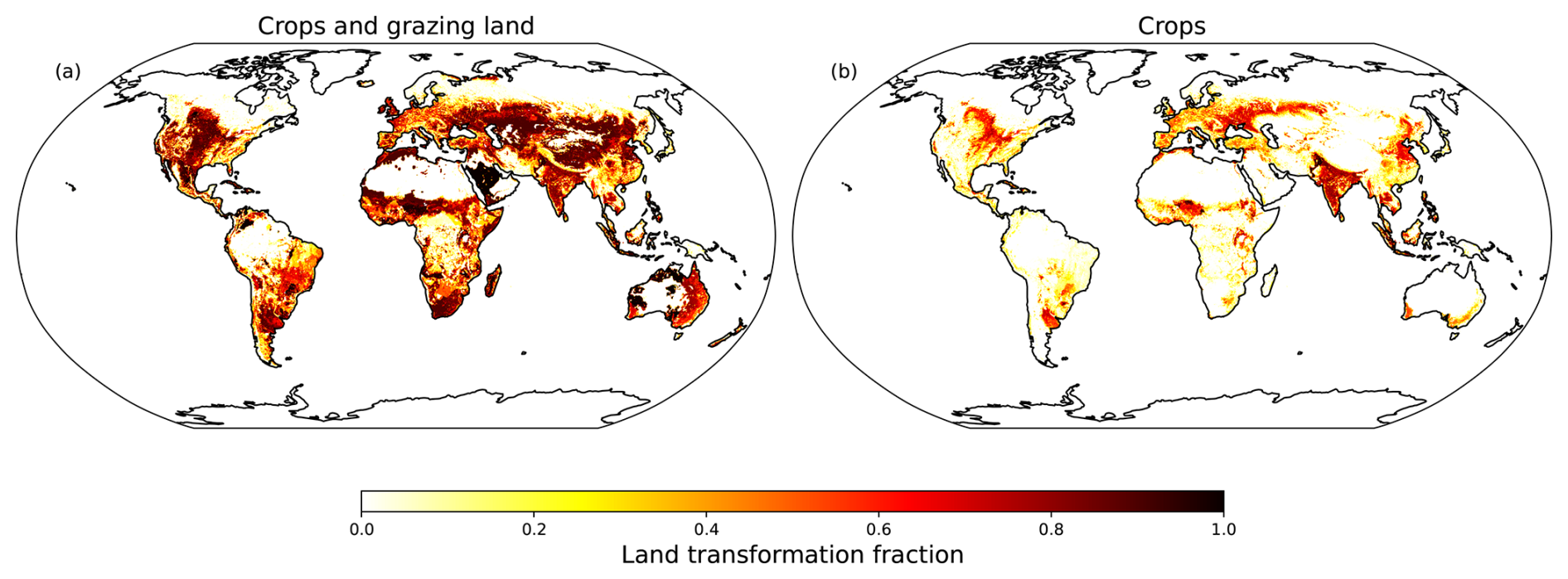
Figure 1 Deforestation maps used for the elimination of tree PFT's in LPJ-GUESS. The maps are derived from HYDE v3.2 based on the year 2015.

All simulations were conducted over 12 years (2000–2011), with the initial 2 years excluded from the analysis to ensure proper spinup and equilibrium state in the analysed data. The vegetation initial states for all simulations were taken from a previous non-chemistry 50 y run under similar atmospheric states. For this study, the simulations were performed in T63L31 resolution, i.e. approximately 1.87° × 1.87°(or approx. 200 × 200 km at the Equator) with 31 vertical levels. The meteorological fields were nudged in the troposphere towards ERA5 data for the respective years 2000–2011. Sea surface temperature (SST) and sea ice coverage (SIC) are also inferred from the ERA5 nudging data spanning 2000 to 2012. Nudging meteorology is essential to avoid deviations in the simulations arising from internal feedbacks involving temperature and climate dynamics. This approach allows us to isolate the effects of perturbed emissions due to land cover change. A limitation of this method is that short-term adjustments in the climate system are constrained and long-term responses, particularly those driven by radiative forcing, are largely suppressed. However, this suppression is primarily not due to nudging, but rather the use of fixed active tracers (based on 2015 levels) in the prognostic radiation scheme, which effectively decouples changes in atmospheric chemistry (e.g. ozone) from meteorology. Consequently, our simulations cannot fully capture climate feedbacks or equilibrium shifts that may arise over longer timescales.

Non-GHG tracers were initialised using climatological data from previous simulations spanning 2000 to 2020. Greenhouse gas mixing ratios, including CO₂, N₂O, CH₄, CO₂, halons, and H₂, were prescribed at the surface level using data from the Chemistry–Climate Model Initiative (CCMI) for the year 2015 (Eyring et al., 2013). CO₂ was fixed in the vegetation scheme, ensuring that variations in CO₂ mixing ratios did not affect plant productivity. Biomass burning emissions were simulated by the BIOBURN submodel, which imports dry matter data (based on 2015) from GFEDv4.1s (Randerson et al., 2015) and employs emission factors from Andreae (2019). Anthropogenic emissions of black carbon (BC), carbon monoxide (CO), nitrogen oxides (NO_x), organic carbon (OC), sulfur dioxide (SO₂), alcohols, and organic gases were based on 2015 and sourced from the Copernicus Atmosphere Monitoring Service (CAMS-GLOB-ANTv6.2 and CAMS-GLOB-AIRv1.1) (Granier et al., 2019).

CAMS-GLOB-ANTv6.2 includes emissions from 14 sectors: power generation, refineries and fuel industries, industrial processes, road transportation, non-road transportation, ships, residential, commercial, fugitives emissions from fuels, solvents application and production, agriculture livestock, agriculture soils, solid waste and wastewater handling, and agriculture waste burning (Denier van der Gon et al., 2023). The PNV run excludes surface emissions from agricultural livestock, agricultural soils, and agricultural waste burning. The DCL run excludes emissions from agricultural soils and agricultural waste burning, while the DCGL run includes all emissions, representing present-day conditions. Agricultural livestock emissions include NH₃, non-methane VOCs (NMVOCs), and NO_x from manure management, as well as CH₄ from enteric fermentation. However, the effect of CH₄ is not considered here, given that methane is prescribed at the lower boundary in our setup. Agricultural soil emissions involve NH₃ and NO_x from agriculture–forestry–fishing activities, rice cultivation, soil emissions, and other sources. Agricultural waste burning emits BC, CO, NH₃, NMVOCs, NO_x, OC, and SO₂ (Denier van der Gon et al., 2023). Anthropogenic emissions are based on 2015 data for all simulated years, with only the activated sectors varying between the runs. Table 1 summarises the experiments, including the anthropogenic emission sectors sourced from CAMS.

Degassing volcanic climatology data were obtained from the AEROCOM project (Dentener et al., 2006). Oceanic emissions and deposition were calculated online using the AIRSEA submodel (Pozzer et al., 2006; Lana et al., 2011; Fischer et al., 2012) for dimethyl sulfide (DMS), acetone (CH₃COCH₃), methanol (CH₃OH) (with an undersaturation of 6 %), and isoprene (C₅H₈). Natural NO soil emissions are calculated in the ONEMIS submodel (Kerkweg et al., 2006; Ganzeveld and Lelieveld, 2004). The agricultural coverage maps used in ONEMIS were updated based on the scenario considered. Specifically, in the PNV scenario no cultivation is assumed while the DCGL scenario includes coverage for both crops and grazing land (Fig. 1a) and the DCL scenario considers only crop coverage (Fig. 1b). Sea salt (Guelle et al., 2001) and dust (Klingmüller et al., 2018) emissions were also calculated online from ONEMIS using corresponding climate states from EMAC. Dry deposition calculations incorporate interactive LAI from LPJ-GUESS, allowing us to evaluate changes in dry deposition fluxes resulting from land cover change.

We note that all scenarios (PNV, DCGL, DCL) use the same meteorological forcing to minimise variability in BVOC emissions. This ensures that any changes in surface temperatures due to aerosol and greenhouse gas forcing are excluded. As a result, we can investigate the impacts on atmospheric composition purely from the perspective of perturbed emissions in the present climate. However, we emphasise that these remain highly idealised simulations, designed to isolate specific chemical responses to land cover change while deliberately neglecting key Earth system feedbacks. While this approach enhances process level understanding, it also limits the extent to which the results can be directly extrapolated to real-world conditions or used for policy-relevant applications.

Table 1 Summary of experiment runs with the corresponding land cover and anthropogenic emissions. Anthropogenic emissions are based on 2015 data for all simulated years, with only the activated sectors varying between the runs.

3 Results

3.1 Present-day land cover

3.1.1 OH reactivity

In this section, we compare tropospheric oxidant chemistry under present-day conditions with a baseline scenario featuring pristine vegetation, i.e. DCGL − PNV. The analysis accounts for changes in BVOC emissions and anthropogenic emissions associated with land cover, i.e. agricultural and livestock activities. In the PNV scenario, annual global isoprene emissions total 418.8 Tg, while monoterpene emissions reach 70 Tg. In the DCGL scenario, emissions are reduced to 307.1 Tg for isoprene and 52.5 Tg for monoterpenes, corresponding to a 25.9 % decrease in total BVOC emissions. It should be noted that the BVOC emissions reported here differ from those reported in Vella et al. (2025), who used a similar model setup. In this study, isoprene emissions were scaled down by 40 %, i.e. reduced to 60 % of their original values, to better reproduce present-day surface O₃ mixing ratios and a global mean tropospheric ozone burden of approximately 350 Tg, in line with satellite-based observational constraints (Gaudel et al., 2018). Global BVOC emissions remain difficult to constrain and we suspect that the MEGAN model overestimates isoprene emissions under present-day conditions. Without scaling, the original emission factors would result in global isoprene emissions exceeding 450 Tg yr⁻¹, which is likely too high.

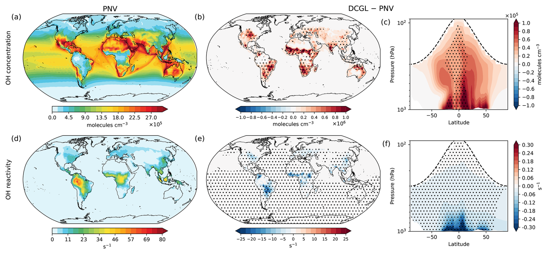
Figure 2 Changes in OH concentration and reactivity. Panels (a) and (d) display the spatial distribution of surface OH concentration and OH reactivity, respectively, under the PNV scenario. Panels (b) and (e) depict the spatial changes at the surface (DCGL − PNV), while panels (c) and (f) show the zonal average across longitudes up to 100 hPa, highlighting OH concentration and OH reactivity changes in the troposphere, respectively. The dashed line in panels (c) and (f) represents the average tropopause height. Averages include day and night OH concentration and reactivity. Dot hatching indicates a statistically significant change based on a two-tailed Student's t test with 95 % confidence.

Figure 2 illustrates the spatial distribution of OH radicals at the surface level of the model. Figure 2a presents the OH surface concentration in the PNV scenario, with the highest concentrations observed in the tropics and mid-latitudes. This pattern is primarily driven by the production of OH from the photolysis of O₃ in the presence of water vapour, along with efficient OH recycling (Lelieveld et al., 2016). Two distinct features are noticeable. First, there are patterns of low OH concentration over tropical rainforests, attributed to the high reactivity of OH with BVOCs, as shown in Fig. 2d. Second, elevated OH concentrations are present along major shipping routes. This enhancement results from the significant NO_x emissions from shipping activities, which increase the formation of ozone and other oxidants, thereby enhancing the production and regeneration of OH over the oceans. The global mean surface OH concentration in the PNV scenario is 1.0 × 10⁶ molecules cm⁻³. Figure 2b shows the change in surface OH concentration in the DCGL scenario relative to PNV, indicating spatial patterns that closely align with the regions of perturbed BVOC emissions due to land cover change (see Fig. S1). In the DCGL scenario, the global mean surface OH concentration increases by 5.9 × 10⁴ molecules cm⁻³, representing a 5.7 % rise. Looking at the zonal annual mean, we find that changes in OH concentrations can extend over the entire troposphere (Fig. 2c), with changes of up to 1.0 × 10⁵ molecules cm⁻³. Most of the changes in surface OH concentration are statistically significant, while the zonal mean shows statistically significant changes across the tropical troposphere. Most of the perturbations occur in the tropics, which is expected given the dominance of tropical rainforests as the primary emitters of BVOCs. Figure 2d–f illustrates the changes in OH reactivity, which represent the rate at which OH radicals react with available trace gases and is mathematically calculated as the reciprocal of the OH lifetime. The reduction in BVOC emissions in the DCGL scenario leads to a global mean decrease in OH reactivity of 14.7 %. As shown in the zonal mean (Fig. 2f), the largest reduction in OH reactivity is observed in the tropical lower troposphere.

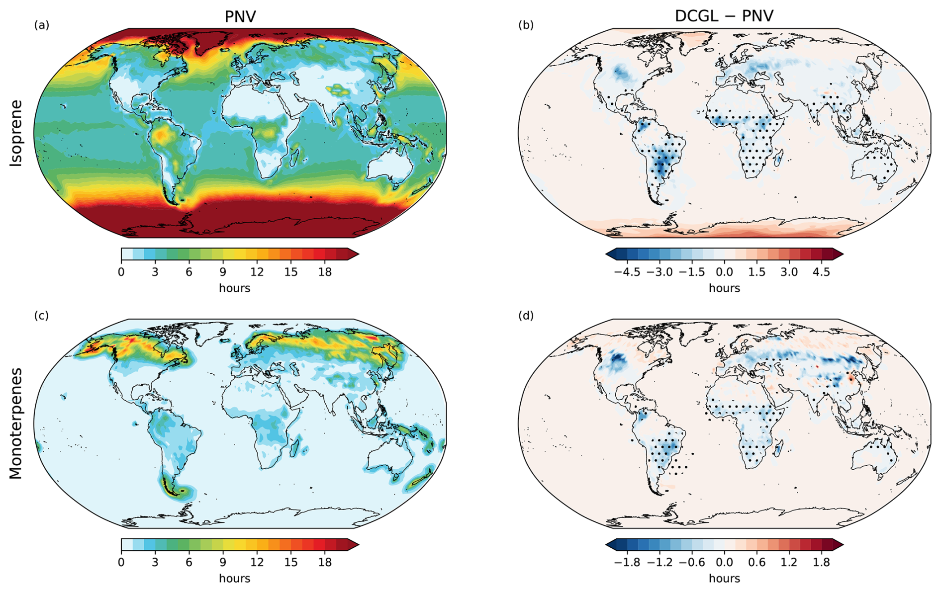
Figure 3 Spatial distribution of isoprene (a) and monoterpene (c) chemical lifetime against OH and O₃ oxidation at the surface. Panels (b) and (d) show the changes (DCGL − PNV) in isoprene and monoterpene lifetimes, respectively. Dot hatching indicates a statistically significant change based on a two-tailed Student's t test with 95 % confidence.

Figure 3 shows the distribution of isoprene and monoterpene lifetimes at the lowest vertical level simulated by EMAC, representing the chemical lifetimes that account for the loss of BVOCs through oxidation by OH and O₃. The lifetime of BVOCs, as well as that of other species discussed later, is calculated as the ratio of the trace gas concentration to its chemical loss rate, as determined using the kinetic chemistry tagging method (Gromov et al., 2010). In the PNV scenario, the annual and global mean isoprene and monoterpene lifetimes are 10.68 h and 61.57 min, respectively. Although the global changes are very small (less than 2 min), in regions directly affected by LCC changes are larger with statistically significant decreases present, both in surface isoprene lifetime (by around 4 h) and monoterpene lifetime (by over 1 h). Here, we also note that the model calculations do not account for chemical loss due to NO₃ and O¹D, which may influence the actual chemical lifetime, especially for monoterpenes. However, oxidation by OH and O₃ remain the dominant pathways for BVOC loss.

3.1.2 Changes in key trace gases

Since OH is a major chemical sink of many atmospheric trace gases, here we address how the changes in BVOC (and therefore OH) and LCC related emissions influence the distribution and chemical lifetime of CO, NO_x, CH₄, and O₃. Figure 4 shows surface distribution and zonal means for CO mixing ratios (a–c) and lifetime (d–f). The simulations indicate that in the DCGL scenario, the global mean surface CO mixing ratio decreases by 7.5 ppbv (6.2 %). Changes in CO are statistically significant over most of the globe. The zonal mean shows CO reductions throughout the troposphere. The surface CO lifetime decreases significantly over deforested regions, contributing to a global reduction in surface CO lifetime by 3.5 d.

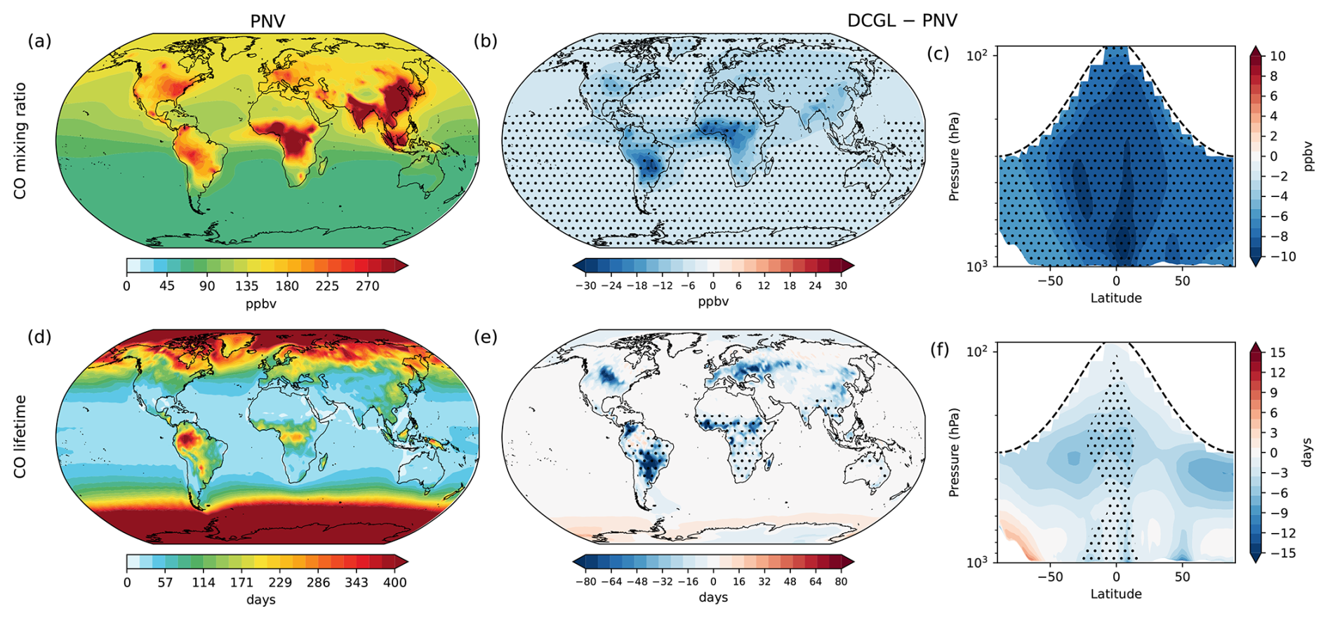
Figure 4 Changes in CO mixing ratios and lifetime. Panels (a) and (d) display the spatial distribution of surface CO mixing ratios and lifetime, respectively, under the PNV scenario. Panels (b) and (e) depict the spatial changes at the surface (DCGL − PNV), while panels (c) and (f) show the zonal average across longitudes up to 100 hPa, highlighting changes in the troposphere for CO mixing ratios and lifetime, respectively. The dashed line in panels (c) and (f) represents the average tropopause height. Dot hatching indicates a statistically significant change based on a two-tailed Student's t test with 95 % confidence.

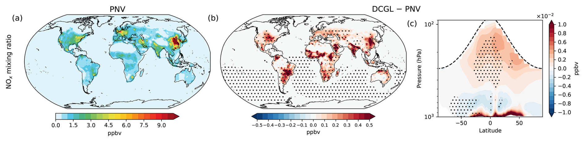
Figure 5 Same as Fig. 4a–c but for NO_x.

Figure 5 shows the distribution and changes in NO_x mixing ratios. We note that both the PNV and DCGL scenarios include anthropogenic surface emissions, which explains the elevated NO_x levels observed over the US, Europe, and particularly China (Fig. 5a). NO_x mixing ratios increase in the DCGL scenario relative to PNV, with average changes up to 1 ppbv (Fig. 5b). Globally, surface NO_x increases by 7.8 %. Figure 5c shows that these changes extend into the upper tropical troposphere. In our simulations, we account for the chemical reactions influencing NO_x surface levels; however, the changes shown here also result from NO_x emission changes due to LCC and variations in natural soil NO emissions driven by the changed vegetation. We estimate a global increase of 2.84 Tg in direct NO_x emissions from agricultural and grazing activities, while soil NO emissions increase by 3.1 Tg yr⁻¹. Figure S9 shows the spatial changes in soil NO emissions.

3.1.3 Ozone production sensitivity

The global mean O₃ surface mixing ratio is 36.6 ppbv in the PNV scenario and 36.0 ppbv in the DCGL scenario, showing a slight decrease of 1.6 % (Fig. 6). Figure 6b illustrates the spatial changes in surface O₃ mixing ratios for DCGL − PNV. Ozone increases by approximately 5 ppbv over tropical South America and Central Africa and around 2 ppbv in Southeast Asia. However, background O₃ decreases, particularly over India and China. The zonal mean plot (Fig. 6c) indicates minimal variations and an overall decrease in O₃ mixing ratios across longitudes.

Changes in canopy densities also lead to changes in dry deposition O₃ fluxes. In these simulations, we calculate dry deposition fluxes interactively using vegetation information from LPJ-GUESS, which includes dynamic changes in vegetation. This approach allows us to account for changes in O₃ dry deposition not only due to variations in O₃ concentrations but also as a result of shifts in canopy distribution and structure. We estimate that in DCGL − PNV, O₃ deposition decreases by 2.4 Tg yr⁻¹ (1.5 %). Spatial changes in O₃ deposition fluxes are shown in Fig. S10. This decrease is largely consistent with the overall decline in O₃ concentrations; however, changes in vegetation (i.e. LAI) lead to a redistribution of where deposition occurs. Regions with reduced canopy density show lower local deposition rates, even if the global burden remains relatively unchanged.

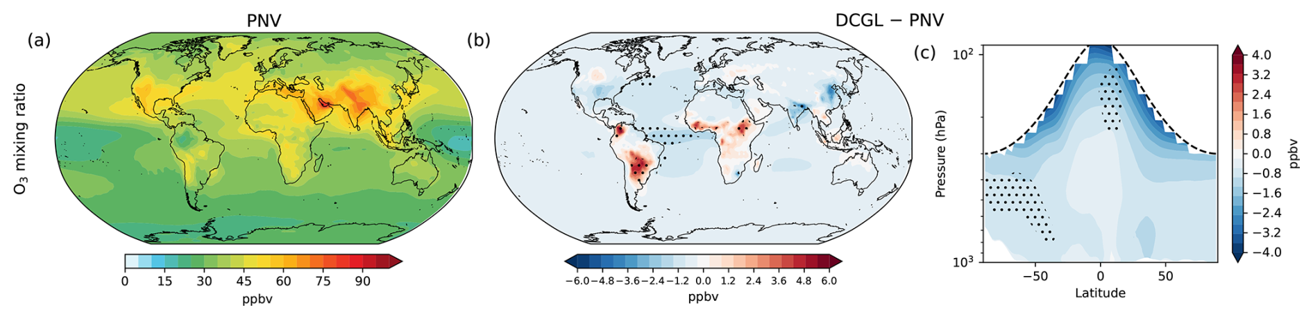
Figure 6 Same as Fig. 4a–c but for O₃.

We explore changes in O₃ formation sensitivity using the metric α(CH₃O₂), which quantifies the proportion of methyl peroxy radicals (CH₃O₂) that react with NO, thereby promoting O₃ formation, relative to those that react with HO₂, which leads to termination of the O₃ production cycle. Ozone formation sensitivity reflects how the balance between these reaction pathways responds to changes in precursor concentrations, such as NO_x and VOCs, and is a key indicator of the chemical regime governing ozone production. This relationship is described by Eq. (1) (Nussbaumer et al., 2021, 2024).

$$\begin{array}{}\text{(1)}& \mathit{\alpha }\left({\mathrm{CH}}_{\mathrm{3}}{\mathrm{O}}_{\mathrm{2}}\right)={\displaystyle \frac{k_{{\mathrm{CH}}_{\mathrm{3}}{\mathrm{O}}_{\mathrm{2}}+\mathrm{NO}}\times \left[\mathrm{NO}\right]}{k_{{\mathrm{CH}}_{\mathrm{3}}{\mathrm{O}}_{\mathrm{2}}+\mathrm{NO}}\times \left[\mathrm{NO}\right]+k_{{\mathrm{CH}}_{\mathrm{3}}{\mathrm{O}}_{\mathrm{2}}+{\mathrm{HO}}_{\mathrm{2}}}\times \left[{\mathrm{HO}}_{\mathrm{2}}\right]}}\end{array}$$

For every model grid box, α(CH₃O₂) was computed using surface values of NO and HO₂, with the rate constants $k_{{\mathrm{CH}}_{\mathrm{3}}{\mathrm{O}}_{\mathrm{2}}+{\mathrm{HO}}_{\mathrm{2}}}$ = 3.8 × 10⁻¹³ exp(780$/T$) and $k_{{\mathrm{CH}}_{\mathrm{3}}{\mathrm{O}}_{\mathrm{2}}+\mathrm{NO}}$ = 2.3 × 10⁻¹² exp(360$/T$) IUPAC (2025).

The sensitivity of O₃ production to its precursors can be characterised by investigating changes of α(CH₃O₂) in response to changes in NO, as shown in Fig. 7. Large increases in α(CH₃O₂) accompanied by small changes in NO, as seen on the steep left part of the curve, indicate NO_x-sensitive O₃ formation. In contrast, very small changes in α(CH₃O₂) despite increasing NO, corresponding to the nearly horizontal section on the right-hand side of the plot, indicate a VOC-sensitive regime. These two regions are connected by an intermediate section of the curve known as the transition regime. Further details on ozone production sensitivity using α(CH₃O₂) can be found in Nussbaumer et al. (2021, 2023). The dominant O₃ production regimes can be visualised in various ways using α(CH₃O₂). For instance, by analysing the α(CH₃O₂) vs. NO curve, one can determine its slope and thus infer the dominant regime Nussbaumer et al. (2024). Here, we examine the y axis of the curve by fitting a linear function to the points in the α(CH₃O₂) vs. NO plot. Since the y axis (α(CH₃O₂) values) ranges from 0 to 1, y intercepts close to 1 indicate an almost horizontal fit, corresponding to a VOC-sensitive regime. Conversely, y intercepts smaller than around 0.7 represent a steep curve, suggesting a NO_x-sensitive regime. The choice of 0.7 and 0.9 as thresholds is supported by a comparative analysis with the method from Nussbaumer et al. (2024), demonstrating consistency in identifying ozone formation regimes. Furthermore, we conducted sensitivity tests using different threshold values, confirming that these thresholds perform well within the context of our study. However, further investigation is needed to assess the broader applicability of these thresholds. They should not be considered as a universal standard, and caution is advised when applying them in other contexts.

Figure 7a shows the y intercepts for each model grid box, representing the spatial distribution of O₃ production sensitivity. The colour bar is adjusted such that values below 0.7 (NO_x-sensitive regions) appear in purple, values between 0.7 and 0.9 (transition regime) are in grey, and values between 0.9 and 1 (VOC-sensitive regions) are in green. Remote regions with low background NO fall within the NO_x-sensitive regime, whereas more polluted regions are in the VOC-sensitive regime.

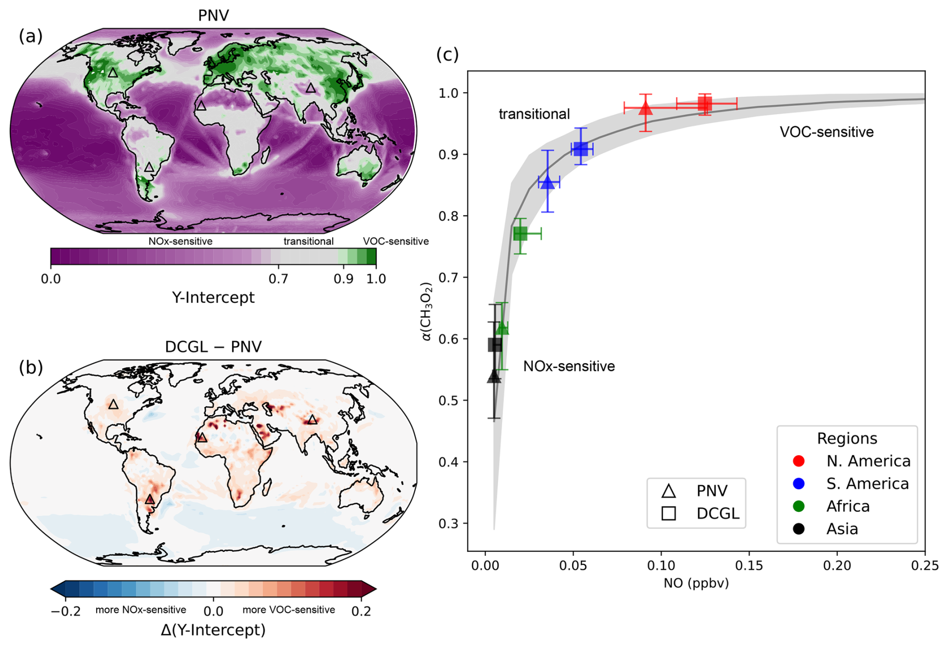
Figure 7 Changes in O₃ production sensitivity are analysed using the relationship between α(CH₃O₂) and NO. Panel (a) illustrates the global distribution of the y intercept in the PNV scenario, while panel (b) displays the change in y intercept (Δy intercept), calculated as DCGL − PNV. Panel (c) presents the medians for α(CH₃O₂) vs. NO, including the background curve derived from medians of all data points, with 25th–75th percentile range shading. It also shows medians (computed over 2° × 2° grid cells) for North America, South America, Africa, and Asia, with the corresponding locations marked by triangle symbols in panel (b). Triangle markers represent results from the PNV run and square markers indicate results from the DCGL run. Both markers include error bars reflecting 25th–75th percentiles.

Figure 7b shows the change in the y intercept for DCGL − PNV, indicating that in regions affected by deforestation, the α(CH₃O₂) vs. NO curve shifts towards larger values for α(CH₃O₂) and NO, suggesting a transition toward the VOC-sensitive regime. Four regions across North America, South America, Africa, and Asia were selected as examples to reproduce the changes in the average α(CH₃O₂) vs. NO under the PNV (triangle markers) and DCGL (square markers) scenarios (Fig. 7c). The plot includes a curve representing the background (i.e. mean of all grid points binned to NO) with a 1σ shading. Across all selected regions, there is a clear shift towards VOC sensitivity. These shifts are, however, not uniform across all regions. We estimate an increase in the ozone mixing ratio of 0.63 ppbv (+1.6 %) in North America, 3.26 ppbv (+10.5 %) in South America, 0.33 ppbv (+0.8 %) in Africa, and 0.34 ppbv (+0.54 %) in Asia. While regions already dominated by VOC sensitivity show relatively little change in α(CH₃O₂) and, consequently, in O₃ formation, more significant shifts occur in regions where the system might transition from a NO_x-sensitive to a VOC-sensitive regime. For example, in South America, we observe a substantial shift in α(CH₃O₂), where ozone production sensitivity is pushed towards VOC sensitivity, resulting in a strong increase in O₃ mixing ratios (+10.5 %) in this region.

3.1.4 Ozone and methane radiative effects

A detailed evaluation of the radiative effects (REs) resulting from changes in the global aerosol burden due to LCC-driven changes in biogenic secondary organic aerosols formed through the oxidation of BVOCs has been presented in Vella et al. (2025). In this study, we focus specifically on the radiative effects arising from changes in O₃ and CH₄ concentrations. Figure 8a illustrates the changes in the top of the atmosphere radiative effects resulting from variations in O₃ concentrations under the DCGL scenario relative to PNV. RE${}_{{\text{O}}_{\mathrm{3}}}$ is computed using a diagnostic radiation call employing interactive O₃ tracer concentrations, thus yielding the instantaneous radiative effect. Land cover change under present-day conditions, compared to natural vegetation, leads to a small global radiative effect of −10 mW m⁻² (cooling), which is a change of less than 1 %.

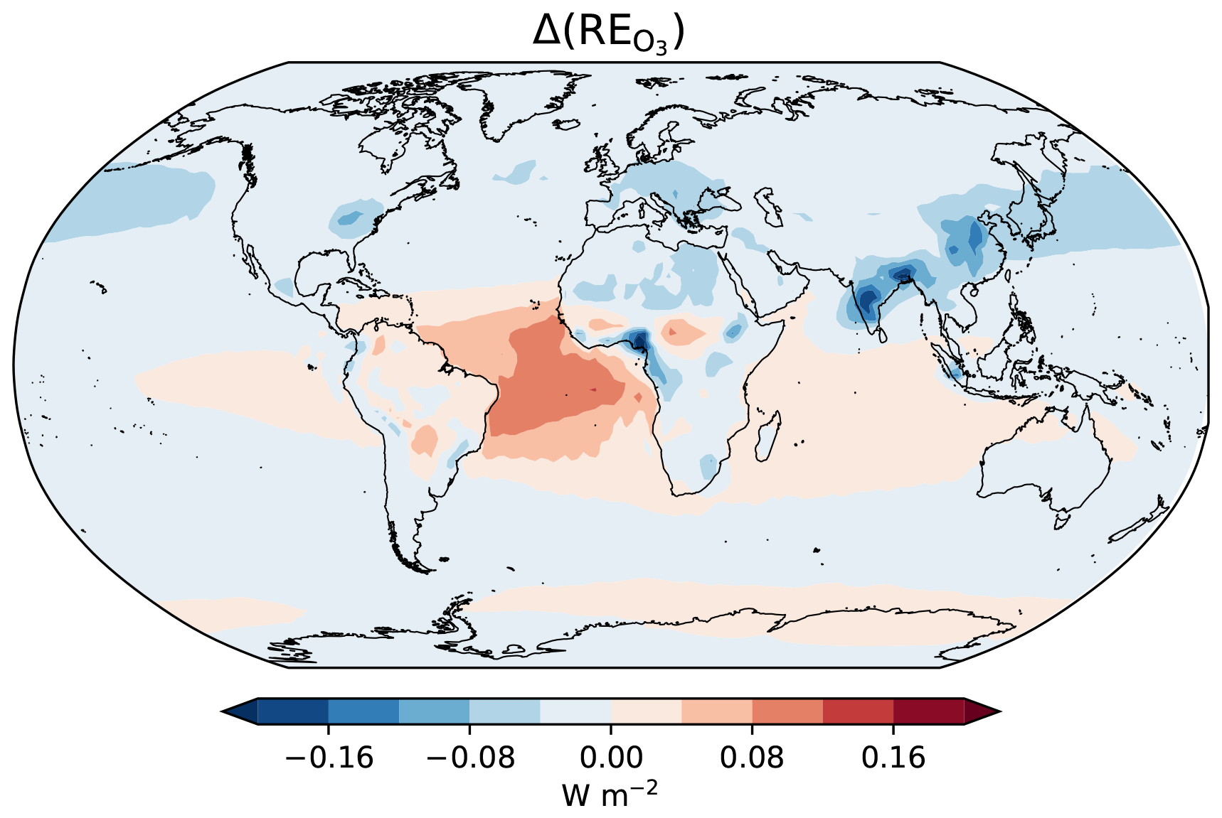
Figure 8 Radiative effects due to O₃ changes from the deforestation (DCGL − PNV) scenario, showing the top of the atmosphere radiative effect (shortwave + longwave).

Differently than O₃, in our simulations, we prescribe surface methane concentrations, meaning that the radiative effect from methane changes cannot be directly evaluated from the model output. We therefore first compute the CH₄ equilibrium mixing ratio, which is the mixing ratio the model is expected to adjust if CH₄ was not prescribed at the lower boundary.

$$\begin{array}{}\text{(2)}& [{\text{CH}}_{\mathrm{4}}{]}_{\text{eq}}=[{\text{CH}}_{\mathrm{4}}{]}_{\text{ref}}\cdot {\left({\displaystyle \frac{{\mathit{\tau }}_{\text{exp}}}{\mathit{\tau }}}\right)}^f\end{array}$$

where [CH₄]_ref is the simulated CH₄ mixing ratio (i.e. the prescribed CH₄ at the surface consistent with DCGL, as they represent the “observed” present-day, which includes land cover changes), and τ_exp and τ are the CH₄ lifetimes from the perturbed (PNV) and reference (DCGL) simulation, respectively (Fiore et al., 2009). f is a feedback factor that accounts for the influence of CH₄ changes on its lifetime, resulting in subsequent adjustments to the CH₄ mixing ratio. The value of f is estimated to range between approximately 1.2 and 1.5 (Fiore et al., 2009; Voulgarakis et al., 2013; Stevenson et al., 2013; Thornhill et al., 2021; Stevenson et al., 2020). We find that the global mean CH₄ lifetime (against OH, O(¹D), and Cl) is 10.6 years in the PNV simulation, compared to 10.1 years in DCGL, representing a decrease of 165 d (4.3 %). This reduction is primarily due to enhanced OH concentrations in DCGL. With a reference CH₄ mixing ratio of [CH₄]_ref=1.91 ppmv, this suggests a reduction of the global CH₄ mixing ratio to 1.78 ppmv in PNV (based on f=1.5). Following the approach used by Etminan et al. (2016), this corresponds to a stratospheric-adjusted radiative effect (RE) of −50 mW m⁻², reflecting the expected CH₄ decrease due to deforestation.

3.2 Grazing land restoration scenario

In this section, we examine the impacts of restoring all present-day grazing land to its potential natural vegetation, i.e. DCGL − DCL. This scenario represents an extreme case of reforestation, effectively testing the upper limit of biogeochemical reversibility following historical LCC. Figure 9 summarises the atmospheric responses to this large scale reforestation, highlighting key changes in BVOC reactivity, surface trace gas concentrations, and chemical regime transitions. Restoring grazing land leads to a widespread increase in tree cover (+600 Mha), which in turn increases isoprene and monoterpene emissions by 22.5 % and 20.5 % respectively. These changes increase the regional BVOC lifetimes by up to 4 h, particularly in areas where grazing land is replaced by forests (Fig. 9b). Figures 9c–e show the associated changes in surface level CO, NO_x, and O₃. Carbon monoxide increases by 4.6 ppbv (4.0 %), NO_x decreases by 0.02 ppbv (5.0 %), and O₃ increases by 0.02 ppbv (0.7 %). Although these changes are modest in absolute terms, they reflect broader shifts in chemical processes. As shown in Fig. 9f, the y intercept of the α(CH₃O₂) vs. NO curve indicates a shift in the chemical regime, i.e. at the surface, and O₃ production becomes more NO_x-sensitive, especially in regions close to LCC.

To place this scenario in a broader context, it is useful to consider present-day vegetation (DCGL) as an intermediate state between the natural vegetation (PNV) and the reforested world of the DCL scenario. In terms of atmospheric composition and radiative forcing, DCGL shares characteristics with both endpoints. For instance, BVOC emissions and the methane lifetime under DCL partially recover toward values seen in the natural vegetation state (PNV), indicating some degree of reversibility. In contrast, ozone concentrations and their associated radiative forcing remain closer to present-day levels (DCGL), suggesting persistent, non-linear responses. This asymmetry highlights the partially irreversible nature of atmospheric chemistry changes following LCC. Additional plots, similar to those in the main text but for DCGL − DCL, are provided in the supplementary material.

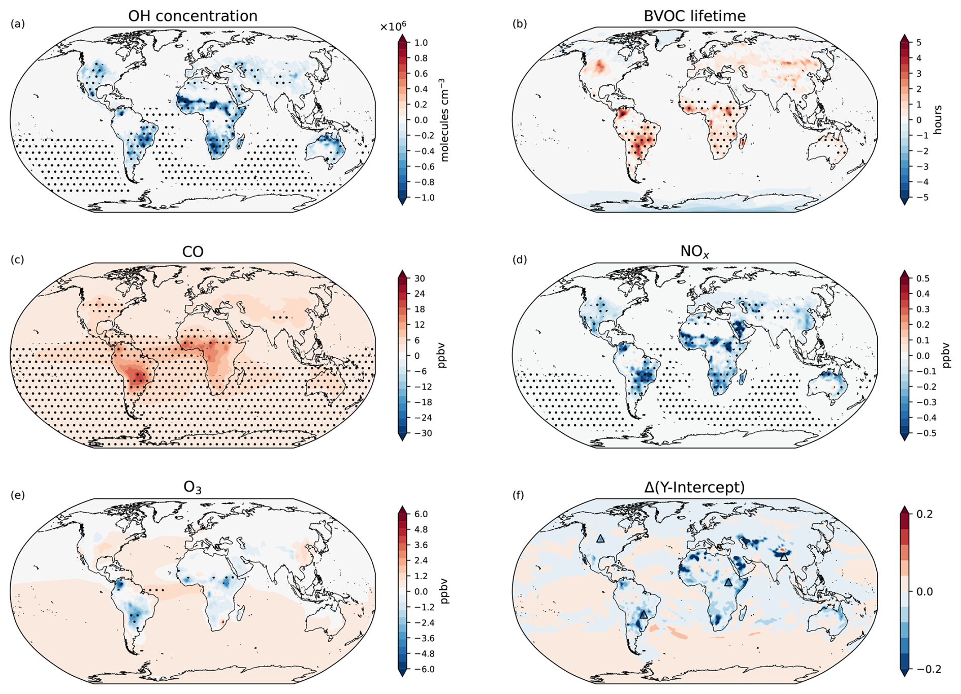
Figure 9 Absolute changes in atmospheric states resulting from the restoration of present-day grazing land (DCGL − DCL). Maps show variations in (a) surface OH concentration, (b) BVOC lifetime, (c) CO surface mixing ratio, (d) NO_x surface mixing ratio, (e) O₃ surface mixing ratio, and (e) changes in O₃ production sensitivity. Dot hatching indicates a statistically significant change based on a two-tailed Student's t test with 95 % confidence.

4 Discussion

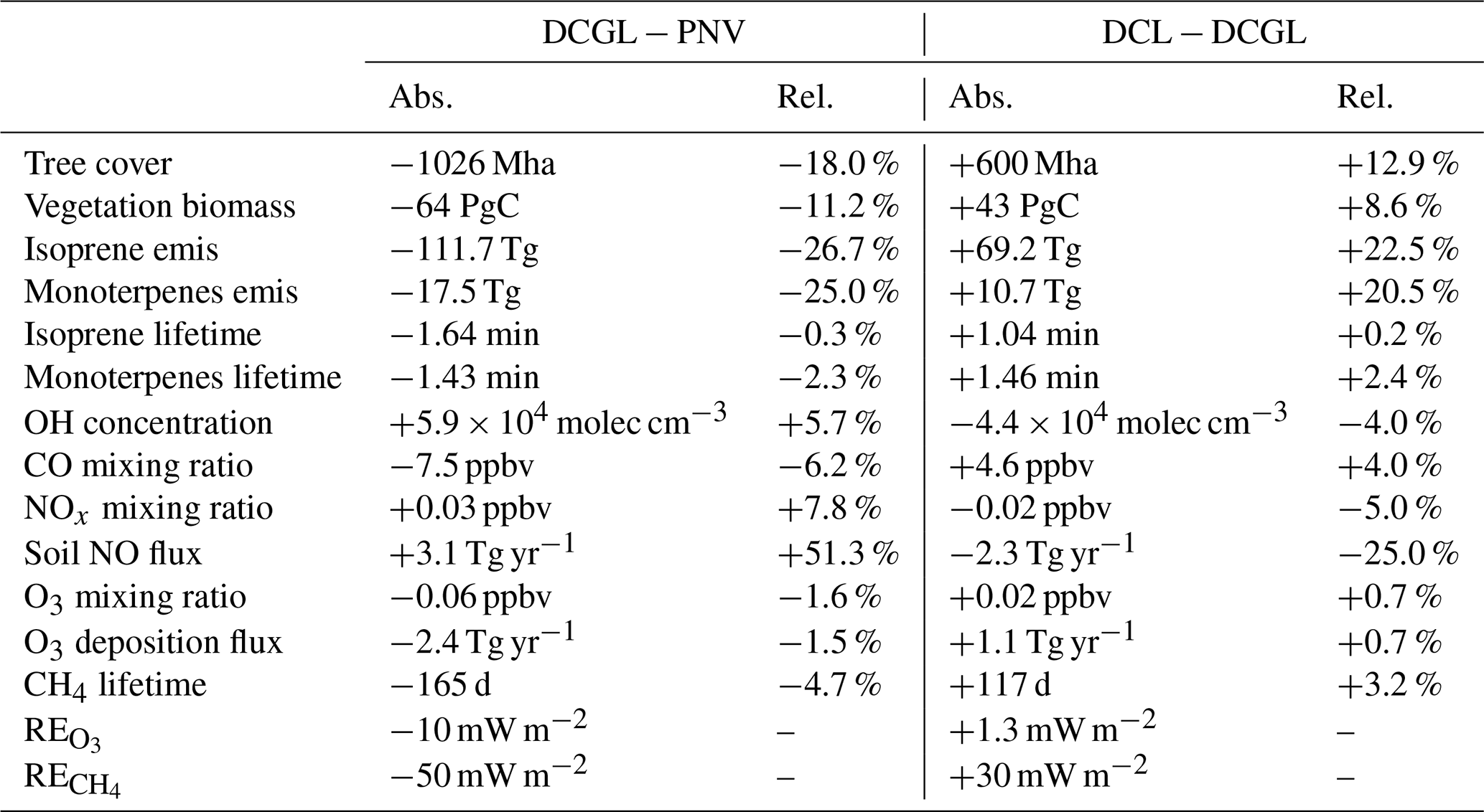
Changes in land cover can substantially impact atmospheric processes and, in turn, the climate system. Numerous studies have explored how land cover changes alter the climate by affecting carbon fluxes, the hydrological cycle, surface albedo, aerosols, and atmospheric chemistry. This study specifically examines the impact of land cover changes on atmospheric composition from perturbed BVOC and anthropogenic emissions associated with LCC. In Vella et al. (2025), we showed that the model setup employed in this work can represent changes in vegetation cover and BVOC emissions in the scenarios considered (i.e. PNV, DCGL, and DCL). This study, which focuses on atmospheric chemistry, introduces two key modifications relative to the setup in Vella et al. (2025): first, aerosol–cloud interactions are not included, thereby excluding aerosol-induced meteorological feedbacks; second, MEGAN-derived BVOC fluxes are tuned to better represent the present-day O₃ burden. All simulations are nudged to observed meteorology, ensuring consistent large scale transport and meteorological conditions across experiments. Additionally, dry deposition fluxes are computed interactively using LAI information from LPJ-GUESS and soil NO emissions were also modified to account for changes in land cover. We emphasise that while vegetation states are fully determined by EMAC prognostic variables, only BVOC emissions and dry deposition fluxes are interactively fed back from the vegetation calculations. This means that other feedbacks associated with land cover change (e.g. changes in evapotranspiration, albedo, roughness length, and aerosols) are suppressed, allowing us to focus solely on the impact of land cover change on oxidant chemistry via perturbed BVOC fluxes and surface emissions from LCC. Table 2 summarises the changes in vegetation and atmospheric states for the different scenarios considered in this work: (i) the difference between 2015 land cover and natural vegetation (DCGL − PNV) and (ii) the impact of restoring grazing land relative to 2015 land cover (DCL − DCGL). Changes are presented in both absolute and relative terms.

Table 2 Changes in vegetation and atmospheric variables for the two land cover scenarios: present-day land cover vs. natural vegetation (DCGL − PNV) and restoration of grazing land vs. present-day land cover (DCL − DCGL). Tree cover, vegetation biomass, isoprene emissions, and monoterpenes emissions are global yearly sums, while OH concentration, CO, NO, O₃ mixing ratios, CH4 lifetime, RE${}_{{\text{O}}_{\mathrm{3}}}$, and RE${}_{{\text{CH}}_{\mathrm{4}}}$ are global yearly means. Concentrations and lifetime are based on the model's surface level, while the radiative effects refer to the top of the atmosphere.

The oxidation capacity of the atmosphere is primarily controlled by hydroxyl (OH) radicals in the troposphere. Consistent with previous studies, our model calculations show the highest OH concentrations in the tropical troposphere, with a global mean (day and night) tropospheric OH of 11.0 × 10⁵ molecules cm⁻³ in the DCGL scenario, representative of present-day conditions. This value is close to the 11.3 × 10⁵ molecules cm⁻³ reported by Lelieveld et al. (2016) and the multimodel mean of (11.1 ± 1.6) × 10⁵ molecules cm⁻³ derived for the year 2000 by Naik et al. (2013).

Present-day land cover, relative to natural vegetation, increases the global mean surface OH concentration by 5.7 % while restoring current present-day grazing land would decrease it by 4.0 %. In both scenarios, surface OH changes correspond to regions where BVOC emissions were perturbed due to deforestation and reforestation. The EMAC results suggest that land-cover-driven BVOC emissions strongly perturb OH concentrations in the tropical troposphere, with relatively strong changes extending to the upper troposphere (Figs. 2c and S2c). While these changes are statistically significant, they remain small relative to the BVOC emissions changes (−25.9 % in the deforestation scenario and +21.3 % in the reforestation scenario). This is due to the efficient recycling of OH radicals, which buffers the global OH burden (Lelieveld et al., 2008). Our simulations include OH recycling chemistry as detailed in Lelieveld et al. (2016). Wu et al. (2012) suggests a global annual tropospheric OH mean of 11.3 × 10⁵ molecules cm⁻³ based on the year 2000. Simulations that account for climate change, CO₂ trends, and land cover change project an OH increase of 1 % in 2050 and a decrease of 2 % in 2100 (Wu et al., 2012). One should note these changes reported in Wu et al. (2012) are primarily driven by the projected increase in BVOC emissions (isoprene: +10 % in 2050 and +25 % in 2100) due to climate warming. Our findings also align with Ganzeveld et al. (2010), who suggest that significant local changes in the atmospheric oxidising capacity are confined to areas influenced by LCC, mostly in the tropics. Scott et al. (2018) estimates that complete global deforestation increases the annual tropospheric mean OH concentration from 13.6 × 10⁵ to 14.6 × 10⁵ molecules cm⁻³ (+7.4 %). This agrees with the 5.7 % increase simulated by EMAC under more realistic land cover changes.

Table S1 highlights the differences in prescribed global annual emission burdens across the simulations. The DCGL − PNV scenario shows increases of 37.1 Tg in CO, 35.25 Tg in NH₃, and 2.84 Tg in NO_x. In contrast, the DCL − DCGL scenario exhibits decreases of 37.1 Tg in CO, 26.58 Tg in NH₃, and 2.64 Tg in NO_x, reflecting the elimination of emissions associated with grazing land practices as these areas are restored.

We report a 7.5 ppbv decrease in the mean annual surface CO mixing ratio in the 2015 land cover scenario relative to pristine vegetation. As OH is the primary sink for CO, the increased availability of OH radicals enhances CO depletion. Notably, this 6.2 % reduction occurs despite an additional 37.1 Tg annual CO emissions burden from grazing land (mostly biomass burning), highlighting the dominant role of atmospheric oxidation in regulating CO levels (Granier et al., 2000). In DCL − DCGL, the 37.1 Tg decrease in surface emissions from grazing land is offset by increased BVOC emissions from reforestation, which lead to a reduction in OH radicals. This reduction in OH limits CO depletion, resulting in a net increase of 4.6 ppbv (4.0 %). We note that changes in CO, modulated by OH, may also feed back to influence OH concentrations, and vice versa. For example, the reduction in CO in the deforestation scenario may partly contribute to the observed increase in OH, while elevated OH levels in turn accelerate CO loss. Nevertheless, we argue that changes in BVOC emissions remain the primary driver of OH variability. OH enhancements resulting from reduced BVOC oxidation likely exert a stronger influence on CO concentrations than CO does on OH, reinforcing the observed decrease in CO.

In the DCGL − PNV scenario, a 2.84 Tg increase in prescribed NO_x emissions leads to a 7.8 % rise in the global mean NO_x mixing ratio. This increase is also partially driven by higher soil NO emissions (+3.1 Tg) due to deforestation, as reduced canopy deposition enhances their release, consistent with (Ganzeveld and Lelieveld, 2004). Despite the increased availability of OH, the substantial rise in NO_x emissions outweighs the enhanced removal of NO_x via oxidation by OH. The increase in surface NO_x also promotes more efficient OH recycling, which can contribute to some of the observed increase in OH concentrations close to the source. Similarly, in the DCL − DCGL scenario, a 2.64 Tg reduction in NO_x emissions, along with a 2.3 Tg decrease in soil NO emissions, dominates surface NO_x levels, leading to a 6.4 % decline.

Land cover changes significantly shift both NO_x and VOC emissions, influencing the O₃ production and distribution. Table 2 confirms that, globally, surface ozone remains relatively unchanged; however, significant regional variations are evident (Fig. 6b). These changes are closely linked to ozone formation sensitivity. As shown in Fig. 6b, urban and polluted areas, which are typically VOC-limited, experience ozone production constrained by VOC availability. In these regions, reduced BVOC emissions lead to lower peroxy radical (RO₂) concentrations, slowing the conversion of NO to NO₂ and ultimately reducing O₃ formation rates. This results in the observed decrease in surface O₃ mixing ratios. Conversely, in rural areas of tropical South America, Africa, and SE Asia, ozone production is more sensitive to NO_x levels. Increased surface NO_x (from farming) enhances NO₂ formation, which photolyses to produce O₃, leading to higher regional O₃ levels. Our analysis using the sensitivity metric α(CH₃O₂) indicates that, under present-day conditions compared to pristine vegetation, ozone production shifts towards a VOC-sensitive regime, except over the Southern Ocean, which appears to shift towards a NO_x-sensitive regime (Fig. 7b). In remote marine environments, such as the Southern Ocean, BVOC concentrations are extremely low, making ozone formation primarily NO_x-sensitive. In these regions, the perturbation of BVOCs has minimal impact on ozone production, and even a slight increase in background NO_x levels can significantly enhance ozone production through NO_x-dependent photochemical processes.

Hotspots where ozone production sensitivity changes drastically were identified and plotted on an α(CH₃O₂) vs. NO curve. The selected locations are Central North America (100° W, 46° N), Southeastern South America (59° W, 28° S), West Africa (11° W, 20° N), and South Asia (91° E, 34° N). Figure 7c confirms that, in these regions, ozone production generally shifts toward a VOC-sensitive regime. While South America and Africa largely remain in the transition regime, a clearer shift is observed in North America, where ozone production moves from the transition regime to a VOC-sensitive regime. In DCL − DCGL, we observe opposite signals (Fig. S7), with ozone production sensitivity shifting toward a NO_x-sensitive regime. Similar trends were presented in Li et al. (2015), who showed that reforestation efforts in southern China increased BVOC emissions. This led to a reduction in surface O₃ by 1.6–2.5 ppbv in rural regions but caused an increase in O₃ peaks by up to 2.0–6.0 ppbv in VOC-limited urban areas. It is important to note that we limit changes in surface emissions related to LCC and do not account for past or future variations in anthropogenic emissions, which would also influence ozone production sensitivity (Wang et al., 2020).

Tropospheric O₃ and CH₄ are potent greenhouse gases with global warming potentials (GWPs) significantly higher than CO₂. As a result, even small changes in the abundance of these gases can impact the climate (Forster et al., 2007). We find that deforestation has had an indirect cooling effect on the climate, with RE${}_{{\text{O}}_{\mathrm{3}}}$ and RE${}_{{\text{CH}}_{\mathrm{4}}}$ of −10 mW m⁻² and −50.0 mW m⁻², respectively. In contrast, restoring grazing land would result in a positive radiative effect of 1.3 mW m⁻² for O₃ and 40.0 mW m⁻² for CH₄. Changes in RE${}_{{\text{O}}_{\mathrm{3}}}$ are not statistically significant; however, this does not rule out the presence of meaningful effects that may be obscured by climate variability.

Scott et al. (2018) estimates a global annual mean tropospheric RE of CH₄ at −70 mW m⁻² and of O₃ at 170 mW m⁻² in a complete deforestation scenario. However, in Scott et al. (2018), RE${}_{{\text{CH}}_{\mathrm{4}}}$ is inferred from changes in steady-state CH₄ concentration, whereas in our calculations, RE${}_{{\text{CH}}_{\mathrm{4}}}$ is derived from changes in CH₄ lifetime due to prescribed surface emissions. Additionally, RE${}_{{\text{O}}_{\mathrm{3}}}$ in Scott et al. (2018) is calculated using a radiative kernel approach that accounts for stratospheric adjustments over the annual cycle, while we compute RE${}_{{\text{O}}_{\mathrm{3}}}$ based on instantaneous radiative effects in the model. Weber et al. (2024) estimates an effective radiative effect (ERE${}_{{\text{O}}_{\mathrm{3}}}$) between 32 and 57 mW m⁻², and ERE${}_{{\text{CH}}_{\mathrm{4}}}$ between 7 and 20 mW m⁻² in a future reforestation scenario. For a fair comparison with the ERE${}_{{\text{CH}}_{\mathrm{4}}}$ reported in Weber et al. (2024), we have to scale our −50 to −43 mW m⁻² to account for additional chemical production of ozone and stratospheric water vapour, and accounting for the negative cloud adjustment including SW absorption by CH₄ (Thornhill et al., 2021; Smith et al., 2018; Etminan et al., 2016). We also calculate the instantaneous RE${}_{{\text{O}}_{\mathrm{3}}}$, excluding any adjustment (e.g. from stratospheric temperatures).

Given the complex response of O₃ to BVOC changes, RE${}_{{\text{O}}_{\mathrm{3}}}$ exhibits high spatial and interannual variability compared to CH₄. As shown in Fig. 8, the top of atmosphere RE${}_{{\text{O}}_{\mathrm{3}}}$ includes regional hotspots corresponding to increases in surface ozone mixing ratios in DCGL − PNV over North America, Europe, and Asia (Fig. 6b). Our findings are consistent with previous work, which shows a negative RE for O₃ and CH₄ linked to deforestation and a positive one linked to reforestation (Unger, 2014; Thornhill et al., 2021). We show that in our model, changes in RE${}_{{\text{O}}_{\mathrm{3}}}$ is not as strong as previously suggested (Scott et al., 2018; Weber et al., 2024). Nevertheless, this discrepancy may partly arise from the slightly different model setups and methods used to estimate the radiative effects.

Based on the reforestation scenario, our results suggest that many biogeochemical and atmospheric responses scale approximately with the extent of tree cover restored. Biomass carbon storage, isoprene and monoterpene emissions, and changes in methane lifetime and RE${}_{{\text{CH}}_{\mathrm{4}}}$ exhibit substantial, though partial, reversibility, indicating a relatively linear response to land cover change. However, the ozone response reveals a notable non-linearity. Despite reductions in NO_x levels, ozone mixing ratios show only modest recovery. This muted response likely reflects a shift in chemical regimes: as shown in Fig. 9f, reforested areas become increasingly NO_x-sensitive, reducing ozone production efficiency even in the presence of elevated biogenic precursor emissions.

5 Conclusions

Understanding the effects of land cover changes on atmospheric composition is essential for assessing the impact of human activities on the Earth system, both historically and in the future. This study provides a detailed analysis of two land cover change scenarios, examining how variations in BVOC emissions and emissions from crop and grazing land affect atmospheric oxidant chemistry. We focus on tropospheric changes in OH radicals, CO, NO_x, O₃, and CH₄, as well as their radiative effects. We find that present-day deforestation relative to pristine vegetation decreases global BVOC emissions. These reductions significantly alter atmospheric chemistry, particularly through their impact on oxidant levels. Global surface OH concentrations increase by 5.7 %, leading to a reduction in the oxidation of CO and a consequent 6.2 % decrease in its surface mixing ratio. In contrast, the global surface NO_x mixing ratio increases by 7.8 %, primarily due to enhanced emissions from cropland and grazing land, as well as increased soil NO emissions from reduced canopy deposition. Ozone changes are more complex, with a global surface mean mixing ratio decrease of less than 1 ppbv (about 1 %). However, significant regional variations occur, driven by shifts in ozone production regimes. Our assessment using the sensitivity metric α(CH₃O₂) indicates a consistent shift towards a VOC-sensitive ozone formation regime in the deforestation scenario. Shorter lifetimes of O₃ and CH₄ result in a small radiative effect of −10 mW m⁻² and −50 mW m⁻² (cooling), respectively. This cooling partially offsets the warming effect from reduced bSOA, which Vella et al. (2025) estimates to be 60.4 mW m⁻². However, a fully coupled Earth system model is necessary to capture the full interplay between these processes, as it enables all relevant feedbacks to be represented. Without such coupling, important secondary effects and compensating mechanisms may be overlooked, potentially leading to an incomplete understanding of the net climate impact. Ongoing land cover change may continue to reduce vegetation cover in pristine forested regions. In areas with low background concentrations of nitrogen oxides, such changes can promote further increases in surface ozone levels due to a shift toward VOC-sensitive ozone production. Increased BVOC emissions from large scale reforestation influence atmospheric oxidant chemistry in a manner largely opposite to deforestation, though with weaker intensity. However, the ozone response exhibits a marked non-linearity.