Extreme concentric gravity waves observed in the mesosphere and thermosphere regions over southern Brazil associated with fast-moving severe thunderstorms

Three groups of intense concentric gravity waves (CGWs) lasting over 10 h were observed by an airglow imager at the Southern Space Observatory (SSO) in São Martinho da Serra (29.44° S, 53.82° W) in southern Brazil on 17–18 September 2023. These CGW events were simultaneously captured by spaceborne instruments, including the Atmospheric Infrared Sounder (AIRS) aboard Aqua, the Visible Infrared Imaging Radiometer Suite (VIIRS) on board Suomi NPP, and the Sounding of the Atmosphere using Broadband Emission Radiometry (SABER) instrument operating on the Thermosphere-Ionosphere-Mesosphere Energetics and Dynamics (TIMED) satellite. The CGWs caused significant airglow radiation perturbations exceeding 24 %, and the distance of the wave centre movement exceeded 400 km. These CGW events were caused by fast-moving deep convection observed by the Geostationary Operational Environmental Satellite-16 (GOES-16). The weaker background wind field during the spring season transition provides the necessary conditions for CGWs to propagate from the lower atmosphere to the mesopause region. The 630 nm emission images were significantly contaminated by specific OH emission bands. The same CGW event was observed propagating from the OH airglow layer (∼ 87 km) to the thermospheric OI 630.0 nm airglow layer (∼ 250 km). The asymmetric propagation of CGWs in the thermosphere may be due to the vertical wavelength changes caused by the Doppler-shifting effect of the background wind field. This multilayer ground-based and satellite joint detection of CGWs offers an excellent perspective for examining the coupling of various atmospheric layers.

1 Introduction

Atmospheric gravity waves (AGWs) are disturbances in the atmosphere caused by various sources, such as convection (Fovell et al., 1992; Piani et al., 2000; Heale et al., 2022; Franco-Diaz et al., 2024), front/jet streams (Fritts and Nastrom, 1992; Plougonven and Zhang 2014; Dalin et al., 2016; Wrasse et al., 2024), wind shear (Fritts, 1982; Pramitha et al., 2015), orography forcing (Nastrom and Fritts, 1992; Wright et al., 2017; Liu et al., 2019; Heale et al., 2020; Geldenhuys et al., 2021; Inchin et al., 2024), and air–sea interaction (Li et al., 2024). AGWs are generated when strong updraughts and downdraughts displace the stable stratification of the atmosphere. As AGWs propagate vertically from the lower atmosphere, their amplitude grows markedly owing to reduced density. When they reach mesosphere–lower-thermosphere (MLT) altitudes, they become unstable and break, dissipating momentum and energy into the surrounding atmosphere (Cao and Liu, 2016; Ern et al., 2022b). This energy deposition makes AGWs crucial drivers of the momentum and energy budgets in the MLT region, fundamentally governing the general circulation, thermal structure, chemical composition distribution, and transport regimes (Fritts and Alexander, 2003; Plane et al., 2023).

Among the many sources of AGWs, convective sources are particularly significant (Alexander and Holton, 2004). They can generate concentric gravity waves (CGWs), the source location of which can be readily determined by the centre position. The backward ray-tracing method, employed for source location determination, can also be applied to circular gravity wave patterns (Ern et al., 2022a). This enables point-to-point studies of their propagation characteristics. The release of latent heat in deep convection acts as a forcing mechanism (Lane et al., 2001), creating CGWs that can propagate upward into the middle and upper atmosphere.

All-sky airglow imagers provide a large field of view and high-resolution observations, making them particularly suitable for observing short-period AGWs in the mesosphere and thermosphere. Through the observational data from airglow imagers, researchers can analyse the propagation characteristics of AGWs, including parameters such as horizontal wavelengths, observed periods, horizontal phase velocities, and momentum fluxes (Swenson and Liu, 1998).

Although the observation of AGWs by airglow imagers has been widely documented in previous studies (Dalin et al., 2024; Nyassor et al., 2021, 2022; Suzuki et al., 2007a; Vadas et al., 2012; Vargas et al., 2021; Wüst et al., 2019; Xu et al., 2015; Yue et al., 2009), dual-layer airglow observations, which involve observing airglow emissions from a hydroxyl radical (OH) layer (∼ 87 km) in the mesosphere and an atomic oxygen emission layer at 630 nm (OI 630.0 nm) (∼ 250 km) in the thermosphere, offer a unique opportunity to simultaneously investigate CGWs in both the mesosphere and the thermosphere. This configuration enables comprehensive studies of gravity wave vertical propagations and their role in vertical atmospheric coupling. However, due to past limitations in observational capabilities, simultaneous detection of CGWs across both the OH and the OI 630.0 nm layers was rare.

In this study, we observed multiple strong CGW events using airglow measurements in southern Brazil on 17–18 September 2023, with a maximum amplitude reaching 24 %, which is far higher than previously reported events with average amplitudes of 2 %–3 % (Li et al., 2016; Tang et al., 2014; Suzuki et al., 2007a). Through ground-based dual-layer and multi-satellite joint observations, we conducted a comprehensive analysis of these events to reveal their role in vertical energy transfer and atmospheric coupling.

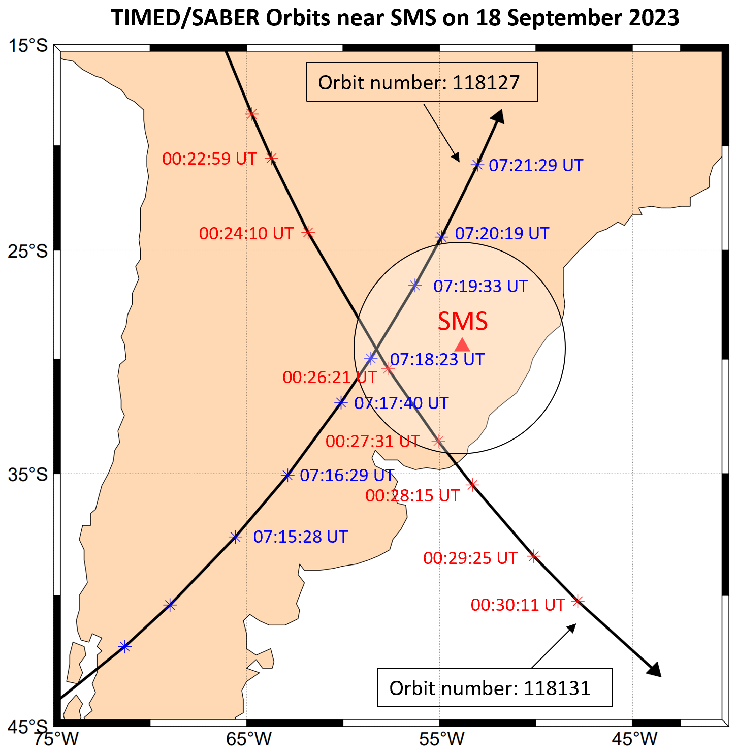
Figure 1 The location of the airglow imager station at SMS (red triangle). The circle on the map gives the effective observation ranges of the OH airglow imager with a 164° field of view. The red asterisks and blue asterisks denote the TIMED/SABER ascending and descending track footprints passing over SMS on 18 September 2023, respectively.

2 Ground-based airglow imager and satellite observation

2.1 Airglow imager

The airglow imager used to observe CGWs is installed at the Southern Space Observatory (SSO), the National Institute for Space Research, in São Martinho da Serra (SMS) (29.44° S, 53.82° W), Brazil. Figure 1 shows the location of the airglow imager station at SMS. The imager has a cooled charge-coupled device (CCD) camera with a Mamiya (focal length of 24 mm) fish-eye lens with a 180° field of view (FOV) and a resolution of 512 pixels × 512 pixels. The imager is equipped with a filter wheel, and the wheel rotates to observe OH (Wüst et al., 2023) broadband emissions (715–930 nm, with a notch at 865.5 nm to suppress the O₂(0, 1) emission) and O(¹D) (630.0 nm, 2.0 nm). The time resolution of the OH airglow image is 112 s, while that of the OI 630 nm airglow image is 225 s. The exposure times of the OH airglow image and the OI 630 nm airglow image are 20 and 90 s, respectively. Airglow observations are conducted when the solar depression angle is less than −12°.

Before effectively extracting the wave parameters, the raw airglow images need to be processed through the following steps. First, a median filter with a kernel size of 17 pixels × 17 pixels was employed to eliminate stars from the raw images (Li et al., 2011). We also removed the CCD dark noise, which was estimated from dark-frame images captured with the shutter closed prior to observations. Second, we corrected for the van Rhijn effect and atmospheric extinction using the approach described in Kubota et al. (2001). The observed airglow intensity I(θ) from the ground is not uniform across different zenith angles. This non-uniformity is due to the van Rhijn effect. Additionally, the observed airglow intensity is influenced by atmospheric extinction, which results from absorption and scattering along the line of sight.

Since airglow observations are subject to the van Rhijn effect, the measured emission intensity at a specific zenith angle (θ) follows the relation (Kubota et al., 2001)

$$\begin{array}{}\text{(1)}& \begin{array}{rl}& I\left(\mathit{\theta }\right)=I\left(\mathrm{0}\right)\cdot V(H,\mathit{\theta }),\\ & V(H,\mathit{\theta })={\left[\mathrm{1}-{\left({\displaystyle \frac{R}{R+H}}\right)}^{\mathrm{2}}{\sin }^{\mathrm{2}}\left(\mathit{\theta }\right)\right]}^{-\mathrm{1}/\mathrm{2}},\end{array}\end{array}$$

where I(0) is the emission intensity at zenith, V(H,θ) is the van Rhijn correction factor, R is the earth radius, and H is the height of the OH airglow layer. The relationship between the observed emission intensity I(θ) – affected by atmospheric extinction – and the true emission intensity I_true(θ) at the airglow layer is described by Kubota et al. (2001):

$$\begin{array}{}\text{(2)}& \begin{array}{rl}& I\left(\mathit{\theta }\right)=I_{\text{true}}\left(\mathit{\theta }\right)\cdot {\mathrm{10}}^{-\mathrm{0.4}\cdot \mathrm{a}\cdot F\left(\mathit{\theta }\right)},\\ & F\left(\mathit{\theta }\right)={\left[\cos \mathit{\theta }+\mathrm{0.15}\cdot {\left(\mathrm{93.885}-\mathit{\theta }\cdot {\displaystyle \frac{\mathrm{180}}{\mathit{\pi }}}\right)}^{-\mathrm{1.253}}\right]}^{-\mathrm{1}},\end{array}\end{array}$$

where a is the atmospheric extinction coefficient, and F(θ) is an empirical equation.

Consequently, the image correction factor, obtained from the combination of Eqs. (1) and (2), takes the following form:

$$\begin{array}{}\text{(3)}& K=V(H,\mathit{\theta })\cdot {\mathrm{10}}^{-\mathrm{0.4}\cdot a\cdot F\left(\mathit{\theta }\right)}.\end{array}$$

The parameter a depends on the atmospheric observing conditions. For the observed CGW events, we treat a as temporally constant. By averaging the images over the observation period, we derive the zenith-angle-dependent airglow intensity profile. The optimal value of a is determined by matching this observed profile with theoretical K profiles across varying a. The fitted value of parameter a is approximately 0.42. Finally, we apply the flat-field correction by dividing the raw images by the corresponding K factor.

Third, we eliminated atmospheric background counts from the images. For background emission, Swenson and Mende (1994) used simultaneous infrared measurements to demonstrate that the background contributes approximately 30 % of the total OH airglow image signal. Similarly, Suzuki et al. (2007b) confirmed this ratio (∼ 30 %) through concurrent OH intensity observations with a spectral airglow temperature imager. In this study, we adopt the same assumption that background emissions account for ∼ 30 % of the total signal.

Then, the original airglow images were spatially calibrated using stars as reference points. Each pixel location (i,j) in the original image was first mapped to a position (f,g) in a standardised coordinate system. Subsequently, the point (f,g) was transformed into geographic coordinates (x,y) using azimuth (az) and elevation (el) angles.

The conversion between original image coordinates (i,j) and standard coordinates (f,g) is defined by a linear transformation (Hapgood and Taylor, 1982):

$$\begin{array}{}\text{(4)}& \left[\begin{array}{c}f\\ g\end{array}\right]=\left[\begin{array}{ccc}{a}_{\mathrm{0}}& a_{\mathrm{1}}& a_{\mathrm{2}}\\ b_{\mathrm{0}}& b_{\mathrm{1}}& b_{\mathrm{2}}\end{array}\right]\left[\begin{array}{c}\mathrm{1}\\ i\\ j\end{array}\right],\end{array}$$

where the coefficients a and b are calculated by applying a least-squares fitting using the observed location of the stars in the original image and their locations in the standard coordinate (Garcia et al., 1997):

$$\begin{array}{}\text{(5)}& \left[\begin{array}{cc}{a}_{\mathrm{0}}& b_{\mathrm{0}}\\ a_{\mathrm{1}}& b_{\mathrm{1}}\\ a_{\mathrm{2}}& b_{\mathrm{2}}\end{array}\right]=\left[\begin{array}{ccc}{\mathbf{1}}^{\mathrm{T}}\mathbf{1}& {\mathbf{1}}^{\mathrm{T}}\mathit{i}& {\mathbf{1}}^{\mathrm{T}}\mathit{j}\\ {\mathbf{1}}^{\mathrm{T}}\mathit{i}& {\mathit{i}}^{\mathrm{T}}\mathit{i}& {\mathit{i}}^{\mathrm{T}}\mathit{j}\\ {\mathbf{1}}^{\mathrm{T}}\mathit{j}& {\mathit{i}}^{\mathrm{T}}\mathit{j}& {\mathit{j}}^{\mathrm{T}}\mathit{j}\end{array}\right]\left[\begin{array}{c}{\mathbf{1}}^{\mathrm{T}}\\ {\mathit{i}}^{\mathrm{T}}\\ {\mathit{j}}^{\mathrm{T}}\end{array}\right]\left[\begin{array}{cc}f& g\end{array}\right],\end{array}$$

where the column vectors i and j contain observed star locations in the original image, while f and g hold their computed normalised coordinates. The vector 1 is a constant-valued column vector with length matching these vectors.

Through a georeference procedure, the standard coordinate images were projected onto geographic coordinates, assuming peak emission heights of 87 km for the OH layer and 250 km for the OI 630.0 nm layer. The spatial resolution of the imager varies significantly with zenith angle. For the OH channel, it is 0.53 km per pixel at the centre of the image and degrades to 39.8 km per pixel at the edge of the image. For the 630 channel, the resolution is 1.53 km per pixel at the centre of the image and decreases to 40.8 km per pixel at the edge of the image.

2.2 GOES, Aqua, Suomi NPP, and TIMED satellite observations

2.2.1 GOES satellite observations

The Geostationary Operational Environmental Satellite-16 (GOES-16) (Schmit et al., 2005), launched in November 2016, is part of the GOES-R Series. The Advanced Baseline Imager (ABI) is the primary instrument on GOES-16, providing high-resolution imagery in 16 spectral bands, including 2 visible channels (0.47 and 0.64 µm), 4 near-infrared channels (0.86, 1.37, 1.6, and 2.2 µm), and 10 infrared channels (3.9–13.3 µm), with a temporal resolution of 10 min and a spatial resolution of 0.5–2 km (Schmit et al., 2017). The brightness temperature (BT), derived from 10.3 µm infrared images from channel 13, is used to study the convection activities during the CGW events.

2.2.2 Aqua satellite observations

The Atmospheric Infrared Sounder (AIRS) (Aumann et al., 2003; Chahine et al., 2006) is an infrared spectrometer and sounder on board the NASA Aqua satellite (Parkinson, 2003). AIRS performs continuous across-track scanning, acquiring data footprints sequentially. The collected data are then organised into 6 min granules. The footprint size of AIRS is approximately 13–14 km in diameter at nadir view, and the scan swath width is around 1765 km (Hoffmann et al., 2014). AIRS is capable of detecting air thermal perturbations induced by GWs with vertical wavelengths longer than 10–15 km and horizontal wavelengths ∼ 50–500 km (Hoffmann and Alexander, 2010). The radiance measurements at the 4.3 µm CO₂ fundamental emission band are particularly sensitive at altitudes of around 30–40 km. In this study, the CO₂ radiance emission band with frequencies ranging between 2299.80 and 2422.85 cm⁻¹ (Rothman et al., 2013) is utilised to measure stratospheric air temperature perturbations.

2.2.3 Suomi NPP satellite observations

The Visible Infrared Imaging Radiometer Suite (VIIRS) instrument, on board the Suomi NPP satellite (Lee et al., 2010; Lewis et al., 2010), is a multispectral scanner capable of capturing high-resolution images in both visible and infrared wavelengths. The day–night band (DNB) of the VIIRS sensor operates in the visible/near-infrared (NIR) range, covering wavelengths from 500 to 900 nm (Miller et al., 2012), which includes three key mesospheric airglow emissions: the O(1S) line at 557.7 nm, the Na doublet at 589.0/589.6 nm, and the OH Meinel band (∼ 600–900 nm). The sensor has a high spatial resolution of 0.375 km at nadir for its imagery bands and 0.75 km for its moderate-resolution bands. The VIIRS sensor has a wide across-track swath width of 3000 km.

2.2.4 TIMED satellite observations

Sounding of the Atmosphere using Broadband Emission Radiometry (SABER) is one of four instruments on NASA's Thermosphere-Ionosphere-Mesosphere Energetics and Dynamics (TIMED) satellite (Russell et al., 1999), launched on 7 December 2001. TIMED focuses on exploring the energy properties and redistribution in the MLT region, providing data to define the basic states and thermal balance of this area. SABER is a 10-channel broadband limb-scanning infrared radiometer (1.27–17 µm). It measures kinetic temperature through CO₂ emissions (15 µm local thermodynamic equilibrium (LTE) below 90 km; 4.3 µm non-LTE above 90 km) with ± 2–5 K accuracy. Simultaneously observing O₃ (9.6 µm), OH (1.6–2.0 µm), and O₂ (1.27 µm) emissions, it quantifies radiative cooling (up to 150 K d⁻¹) and chemical heating (∼ 8 K d⁻¹) in the MLT region with 2–4 km vertical resolution.

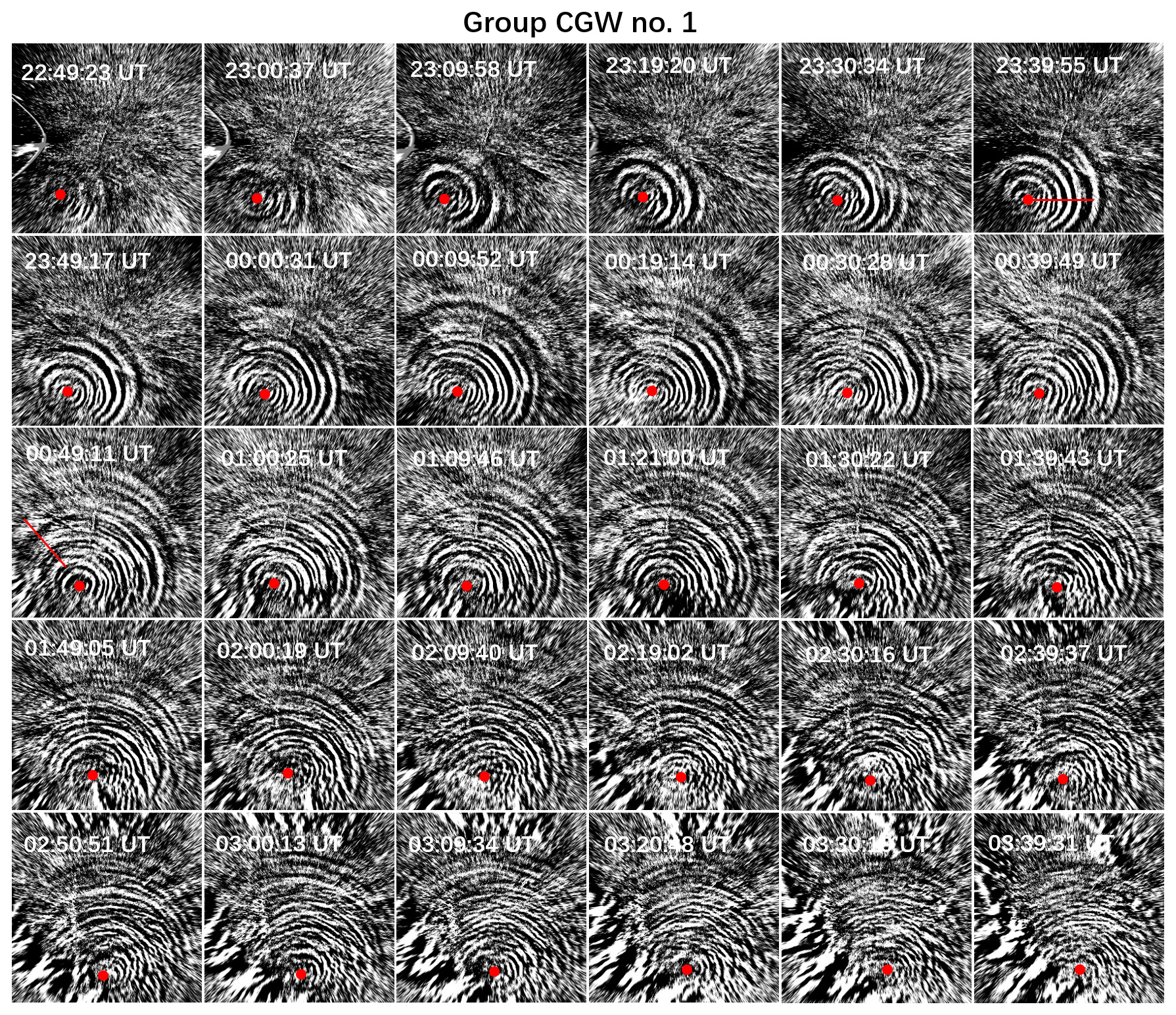
Figure 2 All-sky OH images projected onto an area of 1000 km × 1000 km showing the CGW no. 1 event at half-hour intervals in the SMS station on 17–18 September 2023. The red dots mark the estimated centres of the CGW. The presented images display the corrected OH emission intensity.

3 Observations

3.1 Double-layer all-sky airglow imager observations

3.1.1 Mesospheric concentric gravity waves from OH all-sky imaging observation

Three groups of intense CGWs (wave packet nos. 1–3) were captured by the OH emission channel of the airglow imager at the Southern Space Observatory (SSO) in São Martinho da Serra (29.44° S, 53.82° W) in southern Brazil on 17–18 September 2023. These events initially emerged within the imager's field of view at 22:25:02 UT on 17 September and remained continuously detectable until the cessation of observational recording at 08:35:15 UT on 18 September, thereby spanning an extended duration in excess of 10 h. For more detailed information on the wave propagation status, refer to the Supplement (https://doi.org/10.5446/69990, Li, 2025a). Figure 2 shows the time sequence of CGW no. 1 from 22:49:23 UT on 17 September to 03:39:31 UT on 18 September. CGW no. 1 first appeared in the southwest direction of the station.

The distinct visible concentric wavefronts radiating outward from the centre (red dot in each panel) are indicative of the atmospheric response to disturbances caused by strong convection in the lower atmosphere. Interestingly, the centre of CGW no. 1 continues to move eastward. Between 22:45:38 UT on 17 September and 05:26:13 UT on 18 September, the centre moved approximately 436 km eastward, with an average speed reaching ∼ 65 km h⁻¹. This eastward drift of the wave's centre could be indicative of the influence of prevailing wind patterns and the eastward movement of the convective system itself. The horizontal wavelengths of the GWs at radii of 0–300 km (denoted by the red line in Fig. 2 at 23:39:55 UT) are measured to be (30–82) ± 3 km. The observed period is 9.0 ± 3.5 min, and the observed phase speed is 80–110 m s⁻¹. In the northwest direction (denoted by the red line in Fig. 2 at 00:49:11 UT), we detected larger-scale waves with a wavelength of about 160 km, a period of approximately 16 min, and a phase speed of about 167 m s⁻¹.

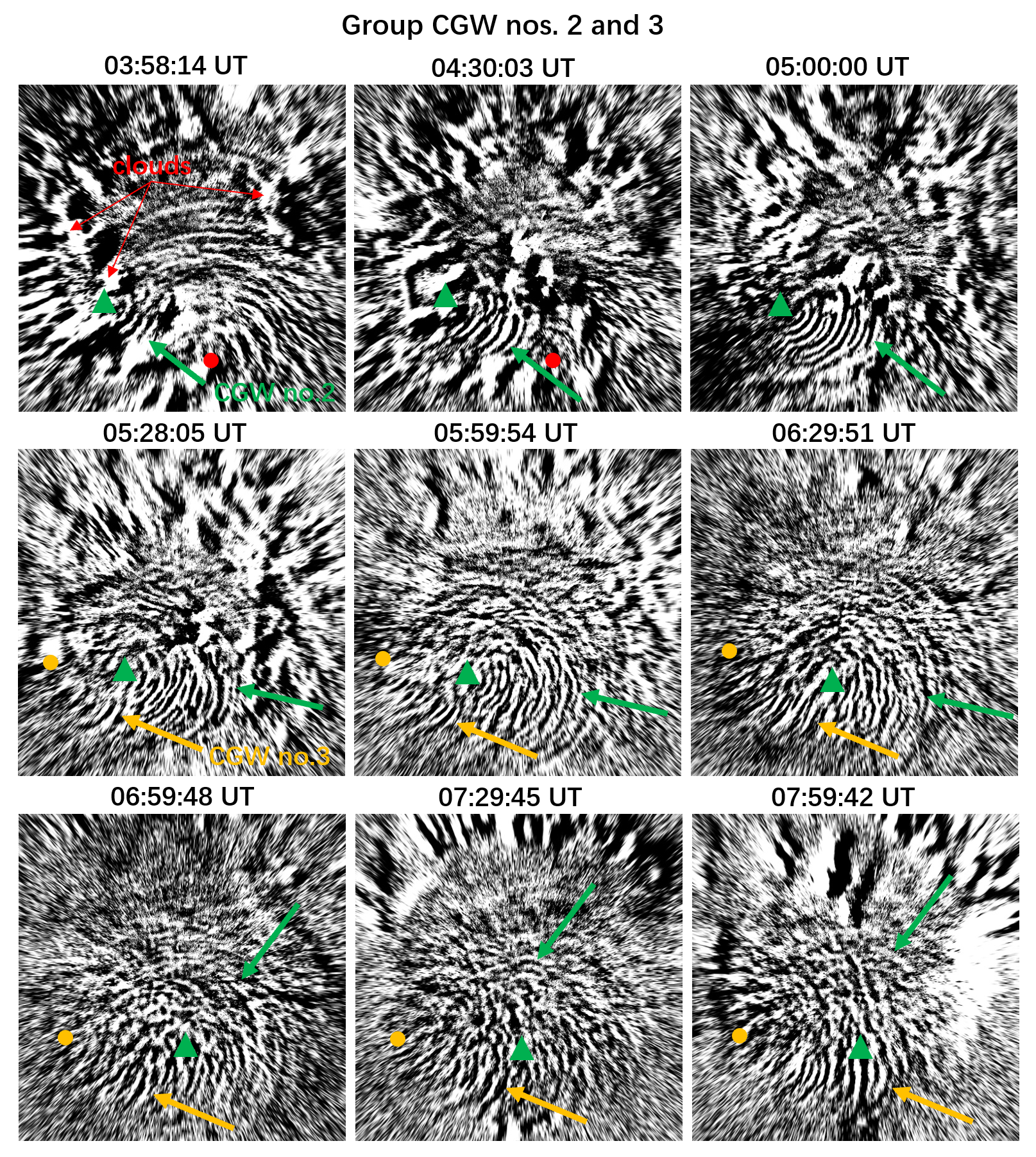
Figure 3 All-sky OH images projected onto an area of 1000 km × 1000 km showing the CGW no. 2 and CGW no. 3 events at half-hour intervals in the SMS station on 18 September 2023. The red dot marks the estimated centre of CGW no. 1, while the green and light blue dots indicate the estimated centres of CGW no. 2 and CGW no. 3, respectively. The presented images display the corrected OH emission intensity.

From 02:00 UT, clouds began forming in the southwestern and western sectors of the station (see Fig. 2). By 04:00 UT, cloud formation extended to the zenith and northern sectors, persisting until ∼ 05:30 UT. Figure 3 shows the time sequence of CGW no. 2 and CGW no. 3 from 03:58:14 UT on 17 September to 07:59:42 UT on 18 September. Despite cloud cover, CGW no. 2 and CGW no. 3 were observed in cloud gaps over the western sector at approximately 03:45:08 and 05:13:06 UT, respectively. For CGW no. 2, horizontal wavelengths range from 22 to 38 km, with a period of 7 ± 1.5 min and a phase speed of 60–78 m s⁻¹. CGW no. 3 exhibits wavelengths of 24–36 km, a period of 6.5 ± 1.0 min, and a phase speed of 72–81 m s⁻¹.

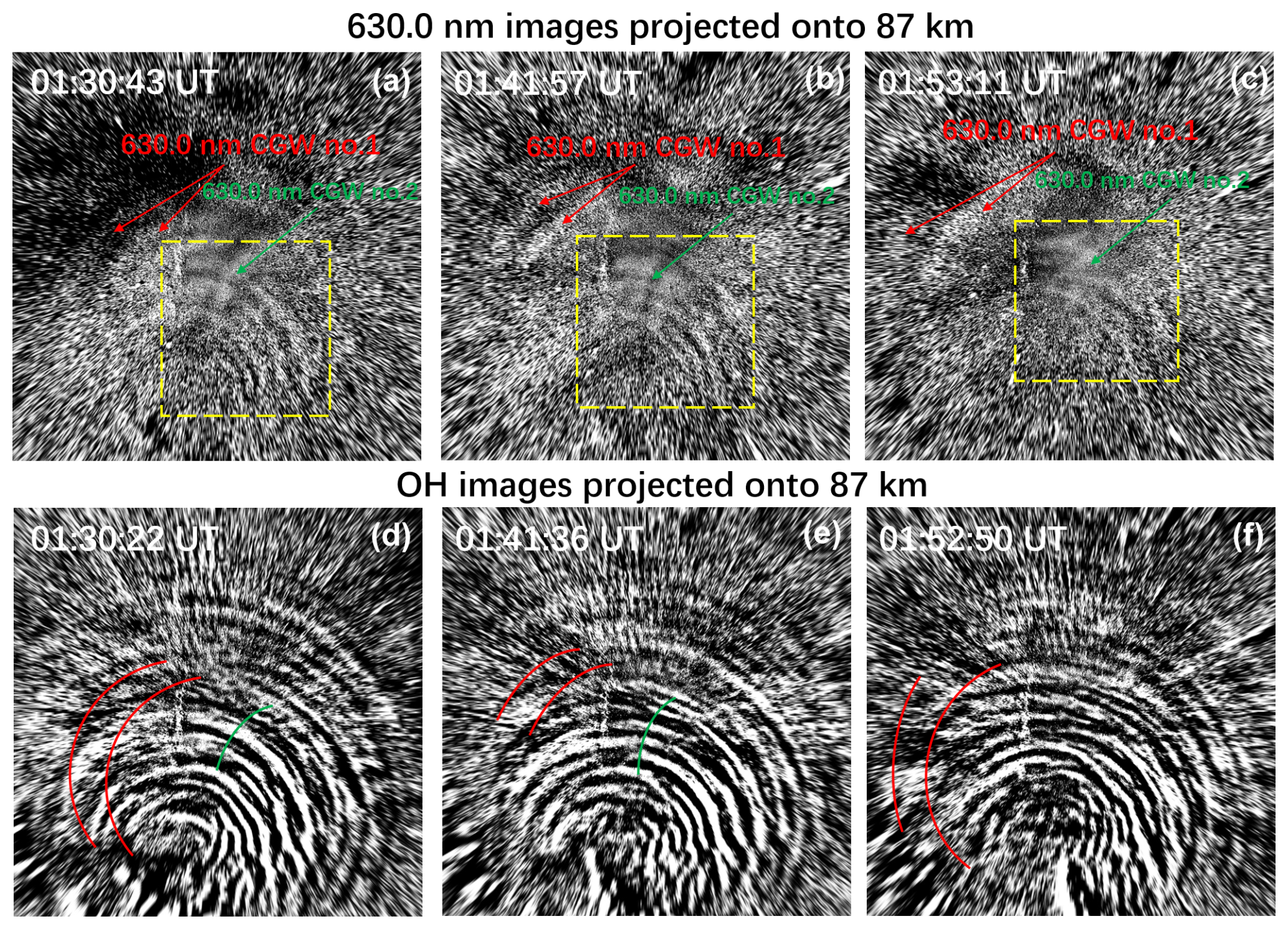
Figure 4 All-sky 630.0 nm images (a–c) and OH images (d–f) were both projected onto an altitude of 87 km with an area of 1000 km × 1000 km. The northeastward-propagating CGW (marked with a dashed yellow box) shows contamination from OH airglow emission. Thermospheric CGWs propagating northwestward confirmed in 630.0 nm images (a–c). The phase fronts of thermospheric CGW nos. 1 (red lines) and 2 (green lines) are superimposed onto the OH images (bottom panel).

3.1.2 Thermospheric concentric gravity waves from all-sky 630.0 nm imaging observation

The 630.0 nm filter used in the imager is a narrowband interference filter with a central wavelength of 630.0 nm and a full width at half maximum (FWHM) spectral width of 2.0 nm. Three spectral lines from the OH (9–3) band lie within the bandwidth of the 630.0 nm filter: the P2(3) line at 629.7903 nm, the P1(3) doublet at 630.6869 and 630.6981 nm, and the P1(2) line at 628.7434 nm (Hernandez, 1974; Burnside et al., 1977; Smith et al., 2013). To determine whether the OI 630 nm airglow image is contaminated by OH airglow emission, we project both the OH airglow image and the OI 630 nm airglow image onto the height of the OH airglow layer. We can clearly see that the OI 630 nm airglow image is contaminated by OH emission, with the CGWs observed in the OH airglow layer being superimposed onto the OI 630 nm airglow image denoted by the dashed yellow boxes in Fig. 4. Thus, we must exercise extreme caution when interpreting disturbances in the thermosphere observed at the 630 nm wavelength, particularly in the absence of concurrent OH airglow measurements, to differentiate whether these disturbances are genuinely thermospheric phenomena or merely artefacts resulting from OH airglow radiation contamination. Notably, thermospheric CGW nos. 1 and 2 (top panel of Fig. 4) were unambiguously observed. Their spatial mapping onto OH images confirms these signals originate from the thermosphere (bottom panel of Fig. 4), excluding OH contamination. Regarding the contamination of 630 nm images by OH emissions and the actual propagation situations of CGWs in the thermosphere, refer to the Supplement (https://doi.org/10.5446/69989, Li, 2025b).

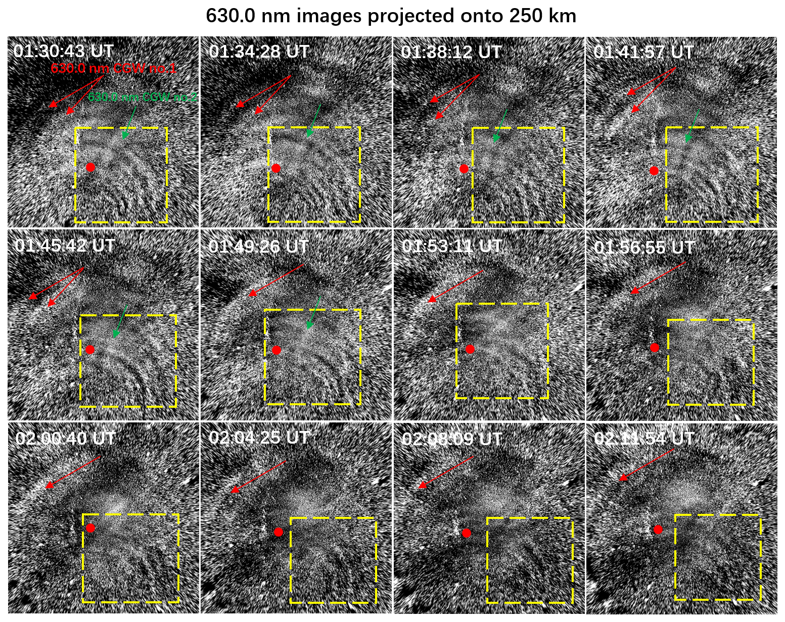
Figure 5 All-sky 630.0 nm images projected onto an area of 2000 km × 2000 km showing thermospheric CGW nos. 1 (indicated by red arrows) and 2 (indicated by green arrows) at approximately 4 min intervals in the SMS station on 18 September 2023. The red dots mark the estimated centres of the thermospheric CGW. The northeastward-propagating CGW (marked with a dashed yellow box) exhibits artefacts influenced by OH airglow emission.

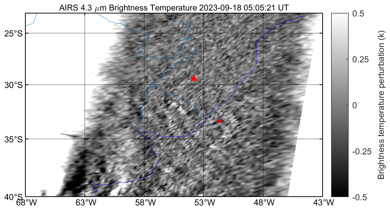
Figure 6 Aqua satellite 4.3 µm brightness temperature observations of CGWs at 05:05:21 UT on 18 September 2023. Brightness temperature is derived from 4.3 µm radiance at an altitude range of 30–40 km. The red triangle and dot mark the SMS station and fitted wave centre, respectively.

Figure 5 presents a series of OI 630 nm airglow emission images projected onto an altitude of 250 km. The ring-shaped arc (thermospheric CGW no. 1) (indicated by red arrows) propagating towards the northwest was identified, with a wavelength of approximately 165 km and a horizontal observed phase speed of about 183 m s⁻¹. There are also observed curved wave structures (thermospheric CGW no. 2) (indicated by green arrows) whose wave fronts are perpendicular to those of the contaminating OH wave fronts. The optical signatures of medium-scale travelling ionospheric disturbances (MSTIDs) in the Southern Hemisphere, as observed in OI 630.0 nm emission images, typically manifest as alternating dark and bright bands aligned along the northeast–southwest direction, propagating in a northwestward direction (Candido et al., 2008). The MSTIDs generally exhibit full FOV coverage, traversing the entire imaging region during their propagation. However, our observations revealed that the thermospheric disturbances first emerged in the zenith region, exhibiting distinctively arcuate phase fronts, suggesting that they were excited by a quasi-point source in the lower atmosphere. The fitted centre of the arc (indicated by a red dot) is located ∼ 320 km to the southwest of the station.

3.2 AIRS and Suomi NPP

Figure 6 shows the AIRS 4.3 µm BT perturbation map over southern Brazil at 05:05:21 UT on 18 September 2023. The AIRS observation reveals large-scale waves propagating northwestward and westward, with a horizontal wavelength of approximately 160 km. The limited spatial resolution of AIRS restricts its detection capability for GWs with short horizontal wavelengths. The relatively weak brightness temperature fluctuations observed by AIRS may result from the instrument's limited sensitivity to short vertical wavelengths (Hoffmann et al., 2014). Consequently, the observed brightness temperature amplitudes are typically much lower than the actual stratospheric temperature fluctuations, especially for convective wave events with short vertical wavelengths. Based on the stratospheric CGW's central position and propagation characteristics, we infer that this wave shares the same source with mesospheric CGW no. 1 identified in the OH all-sky images.

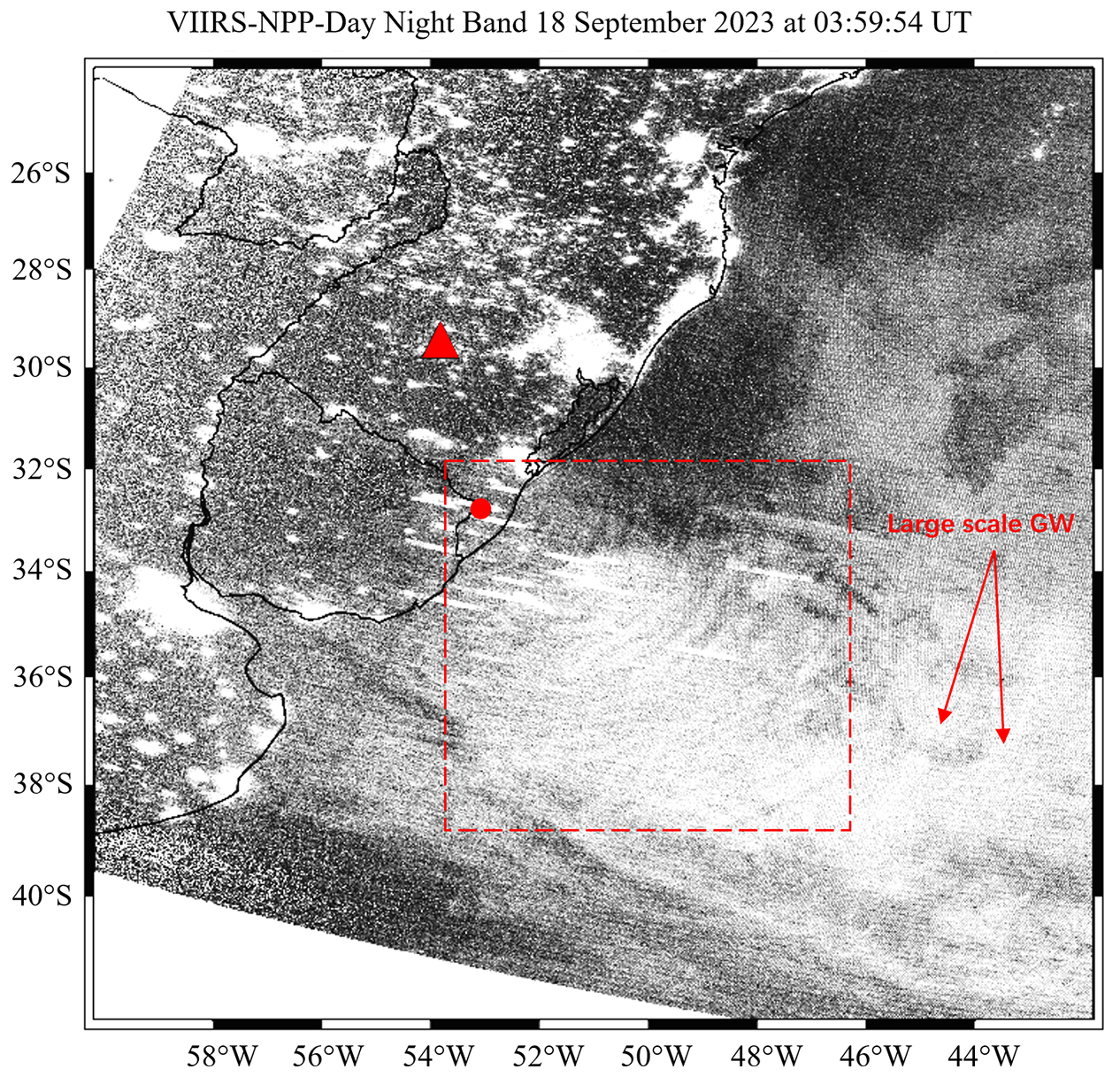
Figure 7 Suomi NPP satellite day–night band radiance observations of CGWs at 03:59:54 UT on 18 September 2023. The red triangle represents the SMS station, and the red dot represents the position of the fitted centre of the CGW.

The Suomi NPP satellite flew over the southern Brazil region during the progression of the CGW events. Figure 7 shows CGWs from the Suomi NPP VIIRS band/DNB measurements at 03:59:54 UT on 18 September 2023. The horizontal wavelengths are primarily distributed within the range of (38–52) ± 3 km (indicated by a dashed red box). In the eastern direction of the small-scale wave region, large-scale waves located at 34–39° S and 43–46° W were detected with a horizontal wavelength of approximately 154 ± 5 km. Due to the interference of urban lighting, the CGW structures were not visible over land.

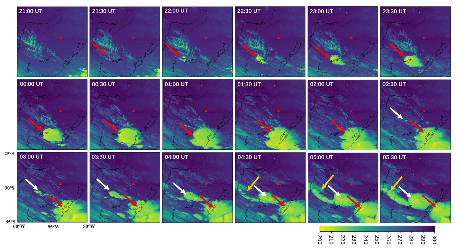
Figure 8 GOES-16 10.3 µm brightness temperature from 21:00 to 05:30 UT on 17–18 September 2023. The brightness temperature is derived from 10.3 µm infrared radiance data from channel 13. The red triangle represents the SMS station.

3.3 GOES observations of convective plumes

Figure 8 shows GOES-16 10.3 µm BT over southern Brazil from 21:00 to 05:30 UT on 17–18 September 2023. The first convective system initially appeared in the southwest direction of the station (indicated by the red arrow) at around 21:00 UT. This convective system continued to move eastward over time and had travelled approximately 400 km by 05:30 UT. This eastward motion explains the observed ∼ 436 km displacement of CGW no. 1 in the mesopause region. The second and third convective systems appeared at approximately 02:30 and 04:30 UT, respectively, and also moved eastward. By 06:30 UT, the three convective systems had merged together. A detailed evolution process of thunderstorm systems is provided in the Supplement (https://doi.org/10.5446/69993, Li, 2025c). The spatial proximity of the three CGW centres to the initiation points of the convective systems strongly suggests that these systems served as excitation sources for the CGWs detected by the airglow imager.

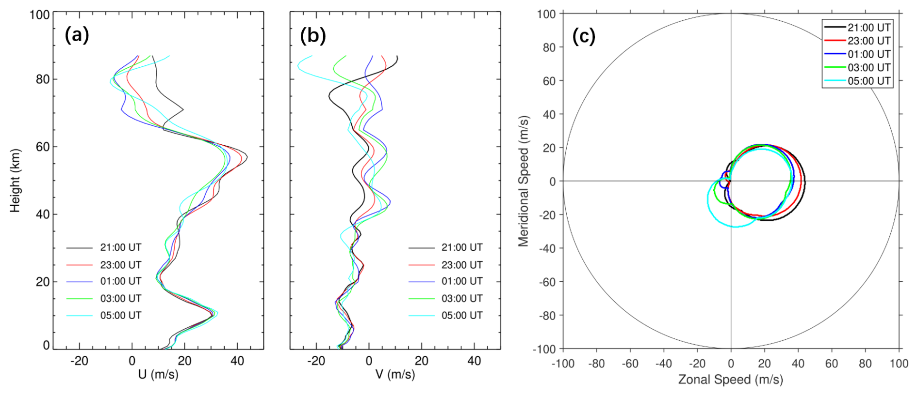
Figure 9 The (a) zonal and (b) meridional wind field profiles from ERA5 (0–70 km) and the HWM14 model (70–87 km) at 21:00, 23:00, 01:00, 03:00, and 05:00 UT, respectively. (c) Two-dimensional blocking diagrams from 0 to 87 km derived from the wind profiles in (a) and (b) on 17–18 September 2023.

4 Results and discussion

4.1 The characteristics of mesopause CGWs

We analysed the background wind field above the station using a composite dataset: the European Centre for Medium-Range Weather Forecasts (ECMWF) ERA5 (Hersbach et al., 2020) for 0–70 km altitude and the Horizontal Wind Model 2014 (HWM14; Drob et al., 2015) for 70–87 km altitude. Figure 9a and b show the zonal wind and meridional wind fields, respectively. Figure 9c presents a critical-level filtering diagram, demonstrating how gravity waves from the lower atmosphere are prevented from reaching the mesopause region when their phase velocities fall within the prohibited range. The diagram reveals a maximum blocking amplitude of approximately 44 m s⁻¹. The results indicate that weaker background winds (producing smaller blocking amplitudes) enhance the vertical propagation of CGWs from the lower atmosphere to the mesosphere. Apart from the moving convective system mentioned above, which is a primary cause of the eastward displacement of the CGW centre observed at the mesopause, the prevailing winds near 10 and 55 km in Fig. 9a also significantly contribute to the eastward movement of the CGW centre.

Figure 10 shows sequential cross sections of OH emission intensity perturbations perpendicular to the CGW no. 1 fronts. The wave amplitudes observed in this study exhibit significantly stronger perturbations, with a maximum relative amplitude of 24 %. In contrast, previous studies have reported average amplitudes that are approximately 2 % (Li et al., 2016; Tang et al., 2014; Suzuki et al., 2007a). Additionally, Smith et al. (2020) reported mean-to-peak wave brightness amplitudes of 10 %.

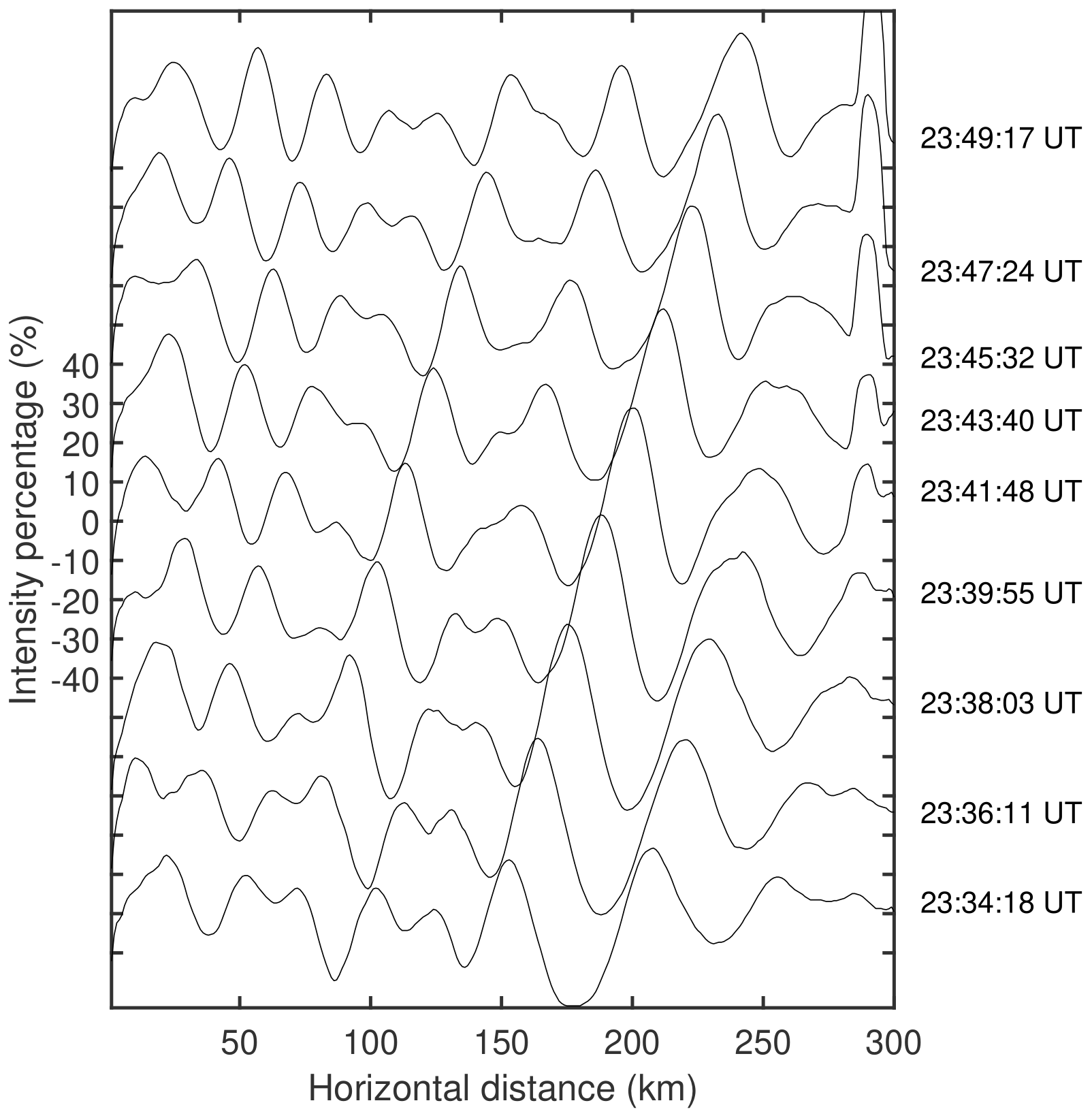
Figure 10 OH emission intensity perturbations perpendicular to the CGW no. 1 fronts (denoted by the red line in Fig. 2 at 23:39:55 UT) from 23:34:18 to 23:49:17 UT on 17–18 September 2023.

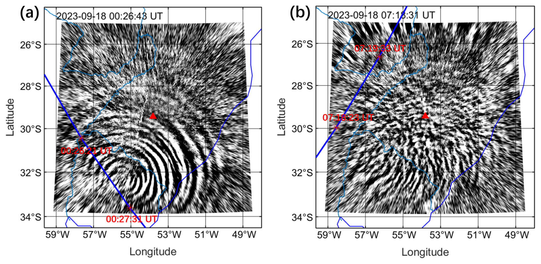
Figure 11 Simultaneous observations of mesopause CGWs using the OH channel ground-based all-sky airglow imager and TIMED/SABER satellite measurements. The red triangle marks the location of the SMS station. The instantaneous field of view of TIMED/SABER is 0.7 mrad by 10 mrad.

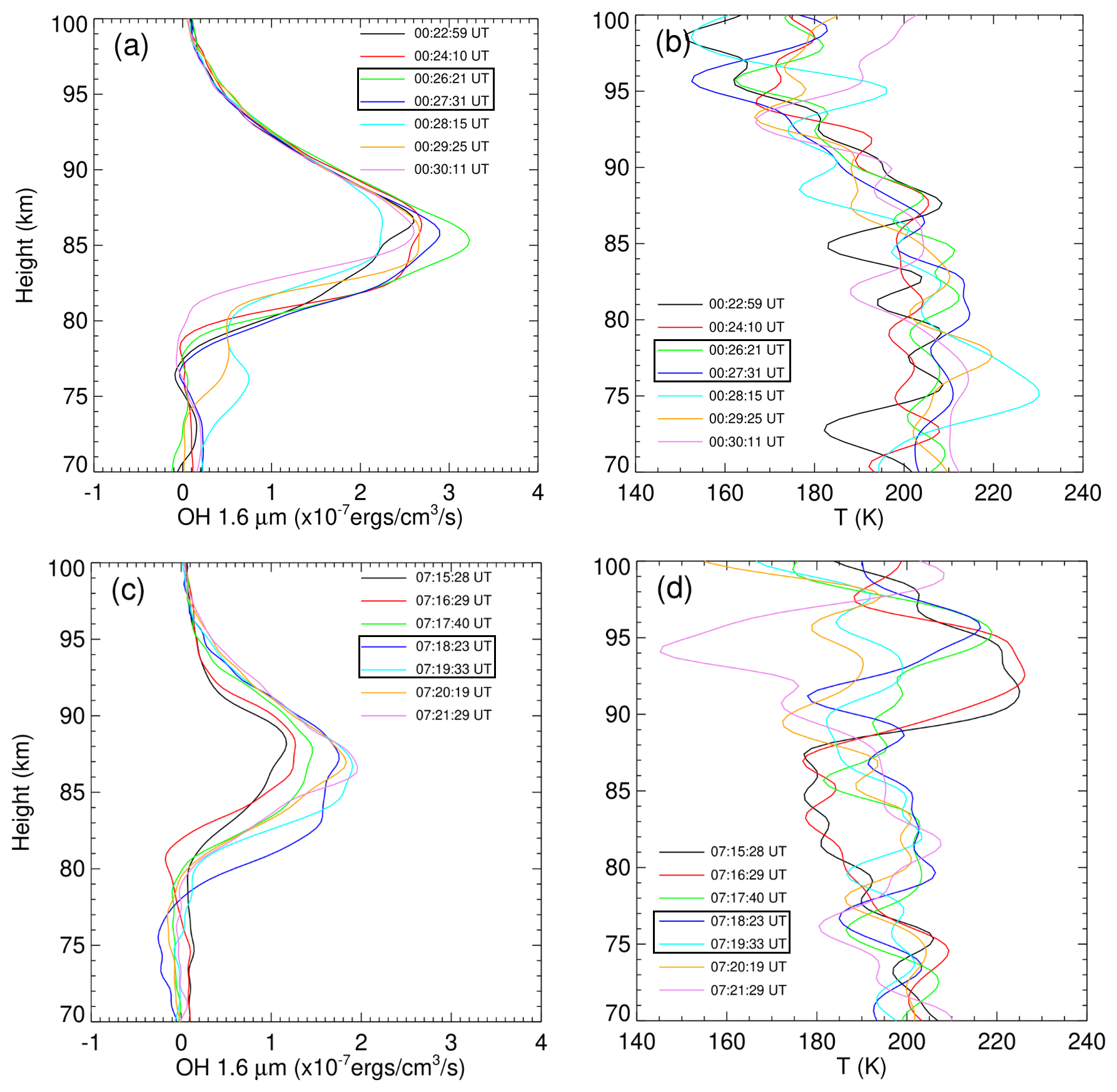
Figure 12 TIMED/SABER (a) OH 1.6 µm emission and (b) temperature profiles (descending track) and (c) OH 1.6 µm emission and (d) temperature profiles (ascending track) on 18 September 2023. Boxed profiles correspond to the satellite's passage through the airglow imager's effective FOV (see Fig. 11).

During the generation and propagation of CGWs, two SABER orbits passed over the station and happened to be within the field of view of the airglow imager, as shown in Fig. 11. The first orbit passes over the station at approximately 00:26 UT, followed by a second orbit ∼ 7 h later at 07:18 UT (Fig. 1). Figure 12 presents seven OH airglow emission and temperature profiles from TIMED/SABER. We observed that the CGWs caused strong disturbances to the airglow layer. We found that the intensity of airglow emission during the first orbit (Fig. 12a) was much stronger than that during the second orbit (Fig. 12c), which may suggest that the intensity of the fluctuations during the first orbit was much stronger than that during the second orbit. In addition to this, we also observed a double-peaked structure in the airglow emission layer. There are weak double-peak structures during the first overpass at 00:24:10 and 00:28:15 UT. In contrast, the double-peak structure is more prominent during the second overpass in the 07:18:23 UT profile.

We can use airglow imaging observations to estimate gravity wave flux (F_M). F_M (Swenson and Liu, 1998; Swenson et al., 1999) is expressed as

$$\begin{array}{}\text{(6)}& F_{\mathrm{M}}={\displaystyle \frac{\mathrm{1}}{\mathrm{2}}}{\displaystyle \frac{g^{\mathrm{2}}}{N^{\mathrm{2}}}}{\displaystyle \frac{m}{k}}{\displaystyle \frac{{\mathit{\omega }}^{\mathrm{2}}}{N^{\mathrm{2}}}}{\left({\displaystyle \frac{I^{\prime }}{\stackrel{\mathrm{‾}}{I}}}\right)}^{\mathrm{2}}{\displaystyle \frac{\mathrm{1}}{{\text{CF}}^{\mathrm{2}}}}\left({\mathrm{m}}^{\mathrm{2}}{\mathrm{s}}^{-\mathrm{2}}\right),\end{array}$$

where $\text{CF}=\mathrm{3.5}-(\mathrm{3.5}-\mathrm{0.1})\exp [-\mathrm{0.0055}({\mathit{\lambda }}_z-\mathrm{6}\mathrm{km}{)}^{\mathrm{2}}]$ is a cancellation factor. λ_z is the vertical wavelength. I^′ is the perturbed airglow intensity. $\stackrel{\mathrm{‾}}{I}$ is the averaged airglow intensity. g is the gravitational acceleration. N is the Brunt–Väisälä frequency derived from TIMED/SABER observations. $k=\frac{\mathrm{2}\mathit{\pi }}{{\mathit{\lambda }}_h}$ is the horizontal wavenumber. λ_h is the horizontal wavelength derived from airglow images. $\mathit{\omega }=\frac{\mathrm{2}\mathit{\pi }{c}_i}{{\mathit{\lambda }}_h}$ is the intrinsic frequency (where c_i is the intrinsic phase speed). $m=\frac{\mathrm{2}\mathit{\pi }}{{\mathit{\lambda }}_z}$ is the vertical wavenumber derived from the GW dispersion relation (Hines, 1960):

$$\begin{array}{}\text{(7)}& m^{\mathrm{2}}={\displaystyle \frac{N^{\mathrm{2}}}{(c-u{)}^{\mathrm{2}}}}-k^{\mathrm{2}}-{\displaystyle \frac{\mathrm{1}}{\mathrm{4}{H}^{\mathrm{2}}}},\end{array}$$

where c is the observed horizontal phase speed of the wave, u is the wind speed in the wave direction derived from HWM14, and H is the scale height from the SABER temperature profile.

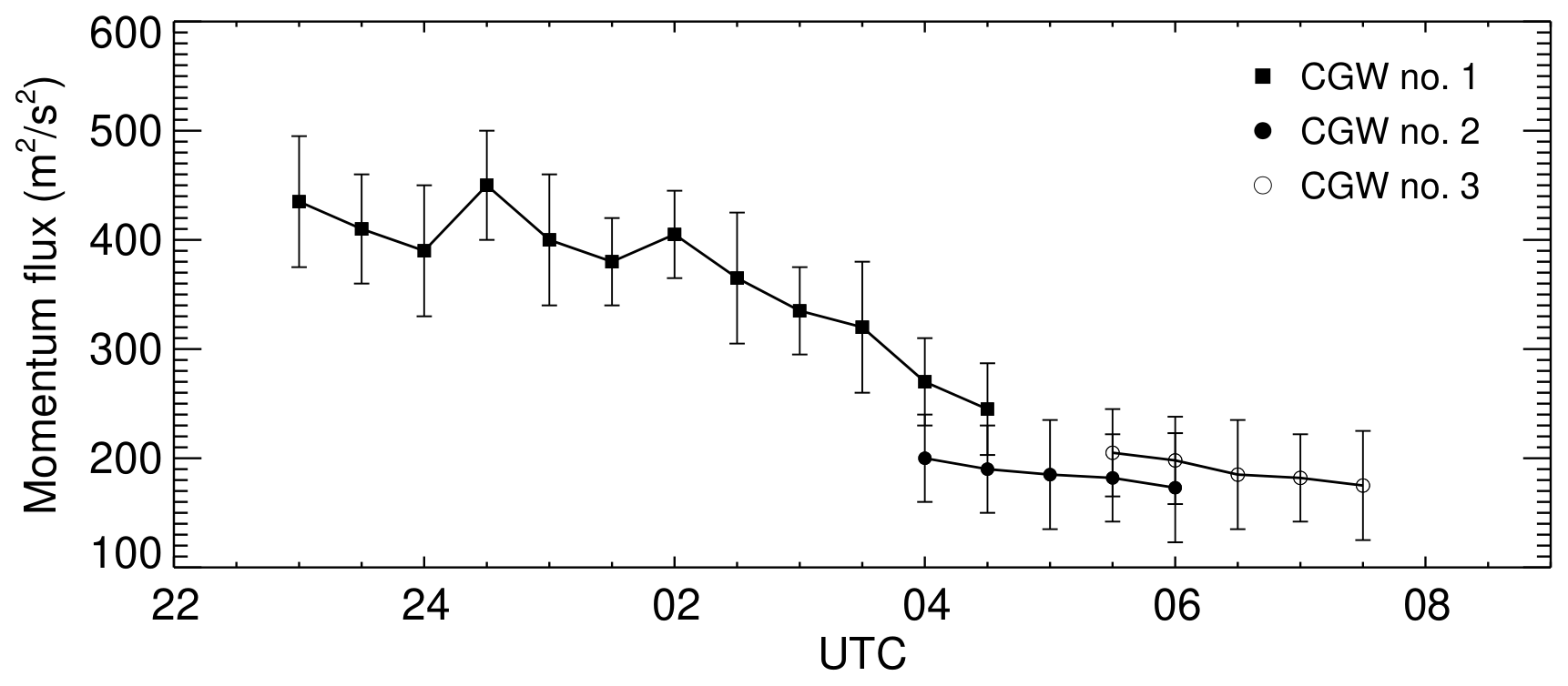
Figure 13 Temporal evolution of vertical flux of horizontal momentum from 22:00 to 09:00 UT on 17–18 September 2023.

Figure 13 shows the calculated vertical flux of the horizontal momentum flux of mesopause CGWs in the altitude of the OH layer from 22:00 to 09:00 UT on 17–18 September 2023. We found that CGW no. 1 produced substantially stronger momentum flux (peak value > 450 m² s⁻²) compared to CGW no. 2 and CGW no. 3, which showed similar but weaker magnitudes. These values markedly exceed previous measurements (typically 1–17 m² s⁻² in Li et al., 2016, and Tang et al., 2014) and even surpass the intense event (decaying from 300 to 150 m² s⁻²) reported by Smith et al. (2020). Ern et al. (2018) studied the climatology momentum flux determined from SABER satellite limb sounding data. They find that the GW absolute momentum flux is approximately 1–4 m² s⁻² in the mesopause region. The results reveal that the fast-moving thunderstorm systems generated exceptionally powerful wave activity, transporting substantial momentum and energy into the MLT region. This demonstrates remarkable wave coupling between the lower and upper atmosphere.

We use the following vertical group velocity equation to estimate the time required for the CGWs generated by the convective systems to propagate to the MLT region:

$$\begin{array}{}\text{(8)}& C_{\text{gz}}={\displaystyle \frac{\mathrm{\Delta }z}{\mathrm{\Delta }t}}=-{\displaystyle \frac{Nkm}{(k^{\mathrm{2}}+m^{\mathrm{2}}{)}^{\mathrm{3}/\mathrm{2}}}},\end{array}$$

where Δz and Δt are the vertical distance and propagation time of the CGWs from the troposphere to the airglow layer, respectively. The horizontal wavenumber k is derived from airglow images. The Brunt–Väisälä frequency N and vertical wavenumber m are calculated as the mean value over the atmospheric layer spanning the tropopause to the mesopause. Notably, the background wind and temperature may exhibit significant altitudinal variations, resulting in substantial variations in the CGW vertical group velocity.

The background temperature for calculating the vertical group velocity of CGW no. 1, no. 2, and no. 3 was derived from TIMED/SABER profiles within an effective FOV of the OH imager during the first orbit (Fig. 12b), the average of the first and second orbits (Fig. 12d), and the second orbit, respectively, while wind field data combined ERA5 (0–70 km) and HWM14 (70–87 km). The vertical group velocities of CGW no. 1, CGW no. 2, and CGW no. 3 are estimated to be 27–42, 21–32, and 24–31 m s⁻¹, respectively. This implies that the time taken for CGW no. 1, CGW no. 2, and CGW no. 3 to reach the OH airglow layer (87 km) is approximately 28–44, 37–57, and 38–50 min, assuming the excitation height of CGWs is 15 km. Yue et al. (2013) conducted multilayer observations of convective gravity waves over the western Great Plains of North America and estimated that the time from the convective source to the airglow layer was ∼ 45 min.

4.2 The characteristics of thermospheric CGWs

We further investigated the propagation characteristics of thermospheric CGW no. 1. The vertical group velocity of the thermospheric gravity waves can be estimated using the following approximate relationship: $C_{\text{gz}}\sim -\frac{N}{k}{\cos }^{\mathrm{2}}\mathit{\alpha }\sin \mathit{\alpha }$. α is the zenith angle between the vertical altitude and propagation direction of the CGW phase fronts. The zenith angle α is approximately 61° from Fig. 14a. The buoyancy frequency N is estimated to be $\mathrm{2}\mathit{\pi }/\mathrm{10.35}\min$ at the thermosphere height of 250 km, which is derived from the empirical neutral atmosphere model (NRLMSISE-00) (Picone et al., 2002). The horizontal wavenumber $k=\mathrm{2}\mathit{\pi }/\mathrm{165}\mathrm{km}$. The estimated vertical group velocity is about 54 ± 6 m s⁻¹. Based on the vertical group velocity, we find that the time taken for the gravity waves to propagate from the OH layer and the tropopause region to the thermosphere is approximately 50 ± 5 and 73 ± 8 min, respectively. As discussed above, the OH images and OI images were captured nearly simultaneously to illustrate the contamination effect in Fig. 4. Some of the wave pattern mismatches in Fig. 4 are due to the propagation time required for CGWs to travel from the OH altitude to the OI altitude. Given the thermospheric arrival time of 01:41:57 UT (Fig. 14a), the CGWs were likely excited near the tropopause (∼ 15 km altitude) at approximately 00:28:57 UT (Fig. 14c) and passed through the OH layer (∼ 87 km altitude) between approximately 00:46:57 and 00:56:57 UT. Notably, GWs with comparable scales were observed in the OH layer at around 00:54:48 UT (Fig. 14b), which suggests that they might be the same wave.

As mentioned above, the observed thermospheric CGWs exhibit an asymmetric structure, appearing as arc-shaped waves only in the western and northwestern directions. This asymmetry can be attributed to the Doppler effect of the background wind field, which influences gravity wave detection through wave cancellation. GWs propagating against background wind are Doppler shifted to a larger vertical wavelength and have an increased chance of observation (Li et al., 2016). These GWs suffer little cancellation and can be easily detected by airglow imager GW observations. GWs propagating along background wind are Doppler shifted to a smaller vertical wavelength, causing the wave amplitude to become invisible. As illustrated in Fig. 14d, the eastward zonal wind at 250 km altitude reaches ∼ 90 m s⁻¹. This strong eastward wind likely suppresses the visibility of eastward-propagating thermospheric CGWs in airglow imaging. We use Eq. (5) to estimate that the vertical wavelength of thermospheric CGWs propagating in the northwest direction is approximately 236 km, while that of thermospheric CGWs propagating eastward is approximately 62 km. The Doppler shift reduces their vertical wavelengths, causing them to fall below the detection threshold of the vertically integrated airglow observations, which is approximately 100 km from 200 to 300 km during nighttime (Chiang et al., 2018).

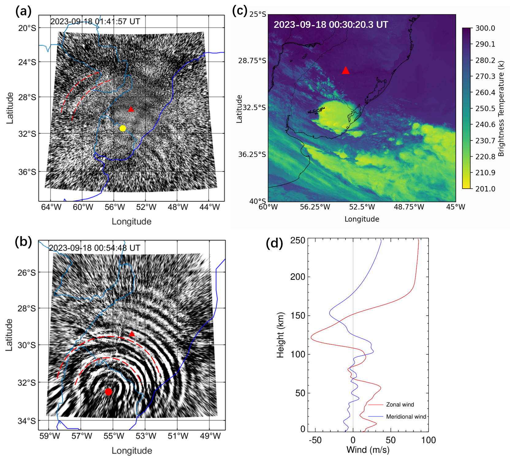
Figure 14 (a) All-sky 630.0 nm imaging observation of thermospheric CGW (dashed red lines) at 01:41:57 UT on 18 September 2023. The yellow dot marks the estimated centre of the thermospheric CGW. (b) All-sky OH imaging observation of mesospheric CGW at 00:54:48 UT on 18 September 2023. The dashed red lines mark the mesospheric CGW with the same scale as the thermospheric CGW. The red dot marks the estimated centre of the mesospheric CGW. (c) GOES-16 10.3 µm brightness temperature at 00:20:20 UT on 17–18 September 2023. The red triangle marks the location of the SMS station. (d) Wind profiles from ERA5 (0–70 km) and HWM14 (70–250 km) averaged between 01:00 and 02:00 UT on 18 September 2023.

5 Conclusions

In this study, we investigated intense CGWs using coordinated dual-channel airglow observations (630.0 nm and OH bands) from the Southern Space Observatory (SSO) in São Martinho da Serra, Brazil, complemented by multi-satellite measurements during 17–18 September 2023. The key findings are summarised as follows.

These unprecedented CGWs exhibited remarkable persistence (> 10 h), extreme amplitude perturbations (> 24 %), and substantial wave centre movement (> 400 km). These wave events were unambiguously linked to fast-moving convective systems observed by GOES-16. The weaker background wind field during the spring season transition was identified as a crucial factor that allowed CGWs to propagate from the lower atmosphere to the MLT region.

The OI 630 nm airglow observations were substantially contaminated by overlapping OH Meinel band emissions (715–930 nm). This contamination leads to spurious apparent vertical coupling, as mesospheric gravity waves (CGWs) are artificially projected onto the thermospheric OI 630 nm emission layer. This cross-layer aliasing effect necessitates rigorous validation protocols when interpreting putative thermospheric disturbances at 630 nm, particularly requiring spatio-temporally collocated OH airglow measurements (e.g. OH (9–3) bands) to discriminate genuine dynamical processes from lower-atmospheric contamination artefacts.

The asymmetric propagation of CGWs in the thermosphere was attributed to variations in vertical wavelength induced by the Doppler effect of background winds. Specifically, the eastward zonal wind at 250 km altitude, reaching approximately 90 m s⁻¹, reduced the vertical wavelength of eastward-propagating CGWs, making them undetectable in airglow imaging observations due to vertical integration effects.

This study reveals intense CGWs originating from deep convective systems that play a dominant role in transferring wave energy and momentum from the troposphere to the MLT region. These waves exhibited exceptional characteristics, including prolonged persistence, extreme amplitude perturbations, and significant horizontal movement, demonstrating their substantial impact on atmospheric dynamics and space weather by (1) seeding travelling ionospheric disturbances (TIDs) that disrupt communications/GPS, (2) triggering plasma instabilities, and (3) altering thermospheric density, affecting satellite drag.

Our coordinated multi-instrument approach, combining dual-channel airglow observations with satellite measurements, provides crucial insights into wave propagation while addressing the challenges of cross-layer contamination in OI 630 nm emissions. These findings significantly advance our understanding of gravity wave dynamics in the upper atmosphere and establish an improved observational framework for studying atmospheric coupling processes.