Building a comprehensive library of observed Lagrangian trajectories for testing modeled cloud evolution, aerosol–cloud interactions, and marine cloud brightening

As the evolution of marine low clouds is sensitive to the current state of the atmosphere and varying meteorological forcing, it is crucial to ascertain how cloud responses differ across a spectrum of those conditions. In this study, we introduce an innovative approach to encompass a wide array of conditions prevalent in low marine cloud regions by creating a comprehensive library of observed environmental conditions. Using reanalysis and satellite data, over 2200 Lagrangian trajectories are generated within the stratocumulus deck region of the Northeast Pacific during summer 2018–2021. By using eight important cloud-controlling factors (CCFs), we employ principal component analysis (PCA) to reduce the dimensionality of data. This technique demonstrates that two principal components capture 43 % of the variability among CCFs. Notably, PCA facilitates the selection of a reduced number of trajectories (e.g., 54) that represent a diverse array of the observed CCF, aerosol, and cloud variability and co-variability. These trajectories can then be used for process model studies, e.g., with large-eddy simulations (LES), to evaluate the efficacy of marine cloud brightening. Two distinct cases are selected to initiate 2 d long, high-resolution, large-domain LES experiments. The results highlight the ability of our LES to simulate observed conditions. Although perturbed aerosols delay cloud breakup and enhance the cloud radiative effect, the strength of such effects is sensitive to “precipitation-aerosol feedback”. The first case is precipitating and shows the potential for “precipitation-driven” cloud breakup due to positive precipitation-aerosol feedback. The second case is non-precipitating with classic cloud breakup of the “deepening-warming” type, highlighting the impact of entrainment.

1 Introduction

Marine stratocumulus (Sc) clouds are an important controller of climate because they cover more than 20 % of the ocean's surface, their albedo is much higher than that of the sea surface, and their effect on outgoing longwave radiation is small (Wood, 2012). Changes in the coverage or albedo of these clouds can therefore have significant impacts on Earth's radiation budget, and biases in their representation in models can produce biases in simulated climate. In addition, a large portion of the global climate forcing through aerosol–cloud interactions (ACIs) occurs in regions of extensive marine low clouds (e.g., Carslaw et al., 2013; Kooperman et al., 2012); accordingly, uncertainty in present-day anthropogenic aerosol radiative forcing is largely attributed to uncertainty in aerosol indirect effects related to low clouds (Forster et al., 2021; Sherwood et al., 2020).

Sc clouds have also been proposed as the potential target for the climate intervention approach known as marine cloud brightening (MCB), one of several methods of solar radiation modification (SRM) that have been suggested as a possible option for deliberately reducing climate warming in the future. MCB would involve injecting sea salt particles from sea water into the atmosphere in regions of marine low clouds. The idea is that these aerosols would mix into the boundary layer air and up to the cloud base, where they would act as cloud condensation nuclei (CCN), resulting in marine low clouds with a larger number of small cloud droplets; this change would enhance cloud albedo (Twomey, 1977), increasing sunlight reflection and cooling climate (Latham et al., 2012). Currently, it is thought that MCB would be most effective when applied to regions of marine Sc clouds (Hill and Ming, 2012). Early research on MCB shows it has the potential to cool the planet, yet significant uncertainties still exist in predicting the efficacy of MCB within global climate models (GCMs), as they do not resolve many of the complex physical processes associated with both unperturbed marine low clouds and their interactions with aerosols (Wood et al., 2017).

Both the present-day effect of aerosols on climate through ACIs and the MCB approach operate by changing the CCN population that is ingested into clouds. The initial response to increasing CCN, either with pollution aerosols or sea salt under MCB, is the Twomey effect (Twomey, 1977), which involves an enhancement of cloud droplet number concentration (N_d) and a resulting increase in cloud albedo if both the cloud liquid water path (LWP) and cloud fraction (CF) are unchanged. The cloud “albedo susceptibility” to the Twomey effect is particularly sensitive to aerosol concentration, such that cloud albedo increases more significantly with lower aerosol concentration (i.e., in a clean environment than in an environment with already-elevated aerosol concentrations) (Platnick and Twomey, 1994).

Importantly, in natural environments, neither LWP nor CF remains constant in clouds with altered N_d. Early research indicated that smaller cloud droplets formed by enhanced aerosols diminish the efficiency of the collision–coalescence process, thereby suppressing precipitation and consequently increasing both cloud cover and cloud lifetime (Albrecht, 1989). More recent studies have demonstrated that ACIs can include additional complex responses, such as increasing the entrainment of air at the cloud top and altering circulation in and adjacent to the cloud. Depending on the background environmental conditions (e.g., the strength of precipitation and entrainment), the cloud responses or “adjustments” in LWP and CF can act to either counteract or amplify the albedo increase produced by the Twomey effect (Glassmeier et al., 2021; Stevens and Feingold, 2009; Wood, 2021). However, the relative importance of different cloud adjustments on a global scale is still not fully understood (Christensen et al., 2022).

Despite the critical role marine low clouds play in climate, both through ACIs in the present climate and for potential MCB, their accurate representation in global climate models continues to be a challenge (Lee et al., 2022; Stjern et al., 2018). The coarse resolution of these models is insufficient for directly simulating the cloud and aerosol processes that drive these clouds' evolution and their responses to aerosol perturbations, which necessitates parameterizations of these processes (Doherty et al., 2022; Erfani and Burls, 2019; Hannay et al., 2009; Zelinka et al., 2017). Large-eddy simulation (LES), on the other hand, proves more effective because it is able to resolve turbulence convection, clouds, and precipitation within the marine boundary layer, or MBL (Berner et al., 2013; Blossey et al., 2021; Erfani et al., 2022; Sandu and Stevens, 2011; Wyant et al., 1997). An objective of this study is to establish an approach whereby the LES model's ability to represent the evolution of marine Sc clouds across a realistic range of background aerosol and meteorological conditions can be systematically tested. The goals of doing so are to advance our understanding of the factors controlling marine low clouds' contribution to Earth's radiative balance, their role in climate forcing by ACIs, and the potential for MCB to cool climate and affect climate risks and, ultimately, to be able to use LES experiments to test and improve the representation of these clouds and both inadvertent (pollution) and intentional (MCB) impacts of aerosols on clouds in global-scale models.

The focus of this study is on regions dominated by Sc clouds and, importantly, includes broad variability in the factors that drive the evolution of these clouds with time. A distinctive characteristic of marine low clouds over eastern oceans is the stratocumulus-to-cumulus transition (SCT), a change in cloud regime that occurs as lower tropospheric air masses in Sc-dominated regions move equatorward, carried by the trade winds. The first theory of what drives the SCT, termed “deepening-warming” (Bretherton and Wyant, 1997; Wyant et al., 1997), describes that the increased sea-surface temperatures (SSTs) experienced during the equatorward movement of a well-mixed Sc-topped MBL cause a deepening and decoupling of the MBL that results in the formation of cumulus (Cu) clouds beneath Sc clouds. Simultaneously, the entrainment of dry air from the free troposphere (FT) intensifies at the top of the Sc layer and therefore leads to the dissipation of these clouds (Bretherton and Wyant, 1997; Sandu and Stevens, 2011; Wyant et al., 1997; Zhou et al., 2015). A more recent theory, a “precipitation-driven” SCT (Yamaguchi et al., 2017), highlights the significant role of aerosols and a positive “precipitation-aerosol feedback”, wherein enhanced precipitation results in a more efficient collision–coalescence process that effectively removes cloud droplets and aerosols from the Sc layer. This clean layer favors the formation of fewer, larger cloud droplets, which in turn intensifies precipitation (Yamaguchi et al., 2017; Wood et al., 2018; Diamond et al., 2022; Erfani et al., 2022).

Previous studies used data from an observational field campaign to both initialize and then test the fidelity of one LES model (System for Atmospheric Modeling, or SAM; see Sect. 2.4) in simulating the SCT in the Northeast Pacific (NEP) region (Blossey et al., 2021; Mohrmann et al., 2019). The Cloud System Evolution in the Trades (CSET) field campaign took place over the NEP in July and August 2015 (Albrecht et al., 2019). To study the movement of air masses, flights first sampled the MBL and lower FT off the California shoreline, and then the air mass was re-sampled 2 d later near Hawaii. Therefore, there are two aircraft intersects for each trajectory providing in situ observations of cloud, aerosol, and meteorological properties. Erfani et al. (2022) selected two Lagrangian trajectories from the CSET campaign and conducted a combination of low- and medium-domain-size LES model runs initialized using baseline and perturbed aerosol concentrations in the MBL and FT in order to explore the sensitivity of cloud evolution, including the SCT, to variations in aerosol concentrations and model domain size. The LES used in that study prognoses aerosol and cloud mass and number concentration; this adds more degrees of freedom, making it more challenging to produce realistic simulations. Nonetheless, the LES did a better job of reproducing the evolution of the aerosol and cloud fields across the 3.5 d simulations in the first case (e.g., L06-Tr2.3) than in the second case (e.g., L10-Tr6.0). The background environmental conditions differed between the two cases: the first case is clean and precipitating, with an initially well-mixed Sc-topped MBL, and the second case is polluted and non-precipitating, with an initially decoupled MBL. As a result, the response of marine low clouds to aerosols and the strength and sign of cloud adjustments differ between the two cases.

The case studies presented by Erfani et al. (2022) inform the analysis presented here, which aims to provide a framework for a more systematic exploration of how aerosols affect low marine cloud evolution. Quantifying these effects requires a comprehensive understanding of cloud responses under the full range of aerosol and meteorological conditions present in the eastern subtropical oceans. Here, we present an approach for creating a comprehensive library of Lagrangian observations and meteorological forcings in order to represent a full spectrum of environmental conditions common in low marine cloud regions. We then apply principal component analysis (PCA) to a range of cloud-controlling factors (CCFs) in order to minimize the data dimensionality and to create a representative phase space of cloud properties. This allows us to identify a subset of cases that are representative of the range of conditions that drive cloud evolution in a given region. In addition, we develop a methodology for routinely initializing and forcing detailed LES experiments with satellite and reanalysis data, rather than relying on aircraft measurements, which are only intermittently available.

Building on Erfani et al. (2022), we perform LES runs with both baseline and perturbed aerosol concentrations for two cases identified from the subset of cases selected using the PCA method described above. These serve as examples to test the performance of our LES and to simulate low marine cloud evolution and ACIs. A later study will use this same approach to more comprehensively analyze LES model performance across an ensemble of simulations based on the subset of cases. The rest of this paper is organized as follows: Sect. 2 describes the observational data and model utilized in the study, along with the innovative statistical approach and design of the LES experiments. In Sect. 3, we explain the outcomes of the statistical analysis. The results of the LES experiments are examined in Sect. 4, a discussion is provided in Sect. 5, and a summary is given in Sect. 6.

2 Data and methods

2.1 Data

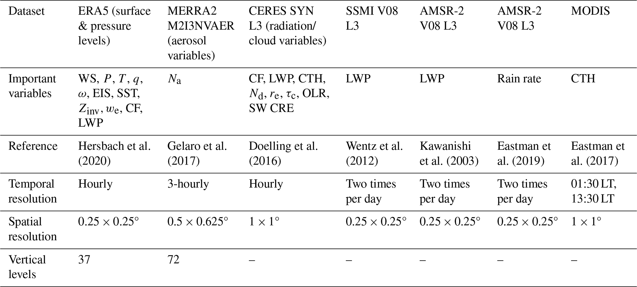
We utilize a variety of reanalysis and satellite data for the Lagrangian study of Sc clouds. Cloud and radiation properties such as CF, LWP, ice water path (IWP), cloud-top height (CTH), and the radiative fluxes were derived from the National Aeronautics and Space Administration (NASA) level 3 Clouds and the Earth's Radiant Energy System (CERES) – synoptic top of the atmosphere (TOA) and surface fluxes and clouds (SYN) (Doelling et al., 2016). Additional sources of satellite-retrieved LWP include the Advanced Microwave Scanning Radiometer (AMSR; Kawanishi et al., 2003) and the Special Sensor Microwave Imagers (SSMI; Wentz et al., 2012). Furthermore, we use CTH estimated from the NASA Moderate Resolution Imaging Spectroradiometer (MODIS) cloud-top temperatures, tuned with cloud-top heights from the Cloud-Aerosol Lidar and Infrared Pathfinder Satellite Observations (CALIPSO; Vaughan et al., 2004) using the algorithm described in Eastman et al. (2017). Estimated warm rain rates are derived from AMSR 89 GHz brightness temperatures tuned using concurrent CloudSat rain profile rain rates (Lebsock and L'Ecuyer, 2011) for marine low clouds, which are available twice daily (Eastman et al., 2019). The European Center for Medium-Range Weather Forecasts (ECMWF) reanalysis version 5 (ERA5) data are used for obtaining meteorological conditions and cloud properties, such as temperature (T), water vapor mixing ratio (q), horizontal wind speed (WS), vertical velocity in pressure coordinates (ω), CF, and LWP (Hersbach et al., 2020). The estimated inversion strength (EIS) is then calculated following the Wood and Bretherton (2006) derivation, as an index to measure MBL static stability. The mass mixing ratio of aerosol species is extracted from the NASA Modern-Era Retrospective analysis for Research and Applications, Version 2 (MERRA2; Gelaro et al., 2017) reanalysis. The MERRA2 reanalysis dataset is generated using the Goddard Chemistry Aerosol Radiation and Transport (GOCART) model, run with assimilated satellite retrievals and meteorological data. Accumulation-mode aerosol number concentration (N_a) is calculated from the MERRA2 mass mixing ratio of aerosol species, with assumed particle size distributions following a methodology described in Appendix A of Erfani et al. (2022). A summary of the datasets used in this study is provided in Table 1.

Table 1 A summary of the datasets used in this study.

2.2 Air mass trajectories

The target region for this study encompasses the Sc cloud deck in the NEP. Six initial locations in this region (see Fig. 1a) are selected as the starting points of forward air mass trajectories that are then used to derive representative cloud properties in this region. All initial locations, except “North”, are based on their use in previous studies. The Sandu 2010 location is selected following Sandu et al. (2010), who analyzed numerous trajectories from this location. The GPCI S9-S12 locations are part of an enhanced observational field campaign, called Global Energy and Water Cycle EXperiment (GEWEX) Cloud Systems Study (GCSS) Pacific Cross-section Intercomparison (GPCI) (Lewis et al., 2012).

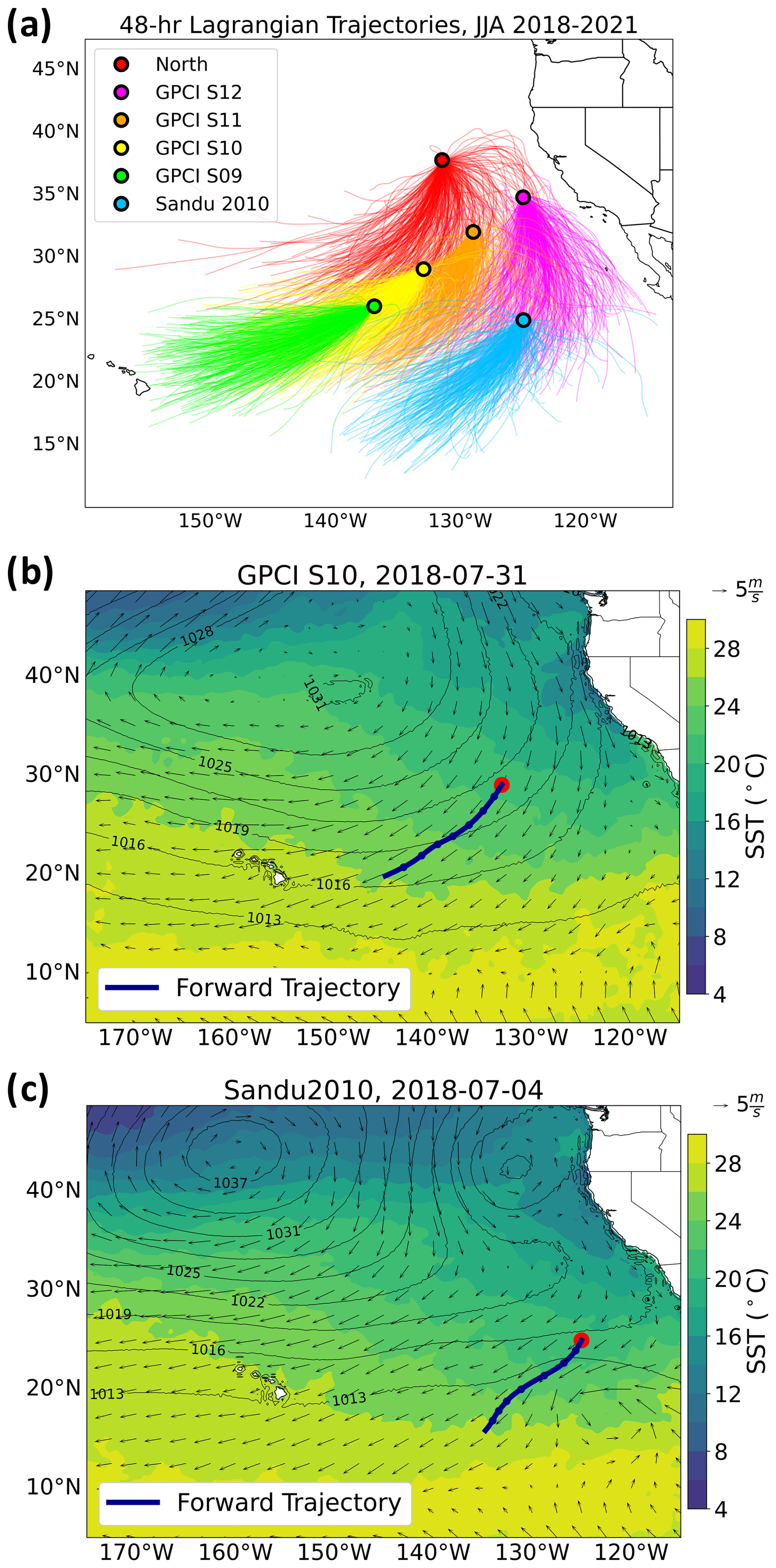
Figure 1 (a) Lagrangian isobaric (950 hPa) 48 h forward trajectories initialized over six select locations in the stratocumulus deck region of the Northeast Pacific for every day during June–August for the years 2018–2021. Excluded are the 4 % of the trajectories that pass close to the coast or over land. See Sect. 2.2 for a description of the initial locations. (b, c) Two Lagrangian trajectories (dark-blue solid lines) used here as case studies for LES modeling. The shaded contours, black contours, and vectors show the ERA5 sea surface temperature, mean-sea-level pressure, and 10 m wind vectors, respectively, averaged for a 48 h period starting from the initial time of the trajectory.

We employ a trajectory generation code developed at the University of Washington (UW) that has been previously applied successfully in several studies of cloud evolution (Bretherton et al., 2010; Eastman and Wood, 2016). This code is used to generate a total of 2208 Lagrangian isobaric (950 hPa) forward trajectories. The resulting trajectories cover a time span of 86 h (3.5 d) and are all from the summer months (June, July, and August, or JJA) in the years 2018–2021. This method uses ERA5 u and v components of horizontal wind to advect air parcels isobarically and assumes minimal vertical motion compared to horizontal motion within the MBL section of stratocumulus deck regions. Bretherton et al. (2010) and Eastman et al. (2017) demonstrated that ECMWF ERA wind fields are appropriate for generating Lagrangian trajectories in the Eastern Pacific. Some widely used trajectory models do not natively utilize ERA5 data in its raw format and require additional preprocessing. In contrast, our trajectory generation code directly uses ERA5 data, which ensures consistency with the “uw-trajectory” Python package utilized later in this study for data extraction.

We acknowledge the inherent uncertainties associated with trajectory methods. Larson et al. (2022) noted that trajectory models, which rely on wind fields, may not always align perfectly with observed cloud motion, possibly due to vertical wind shear. Such wind shear might result in non-negligible horizontal advective tendencies in our quasi-Lagrangian framework because the trajectory is not Lagrangian at all levels (e.g., Blossey et al., 2021). Despite these limitations, isobaric trajectories have been shown to effectively capture the dominant motions in the Sc-topped MBL (e.g., Sandu et al., 2010), and tracers such as CO and O3 exhibited high coherence along such trajectories over a 2 d period during the CSET field campaign (Mohrmann et al., 2019). Our choice of the UW trajectory generation code is motivated by its demonstrated effectiveness in prior research and its compatibility with the ERA5 dataset used throughout this study.

To compile meteorological, cloud, radiation, and aerosol properties along the trajectories, we utilize the uw-trajectory Python package, which was originally developed for the CSET field campaign (Mohrmann et al., 2019) but has since been modified for use with any initial time and location, provided the necessary datasets are available. The uw-trajectory package provides data averaged over a 2° × 2° box centered on each trajectory point at each time. This sample size is consistent with previous studies (e.g., Eastman and Wood, 2016; Eastman et al., 2017; Mohrmann et al., 2019) and ensures that sufficient data around each trajectory point are selected based on the spatial scales of the satellite cloud and reanalysis meteorological properties, as shown in Table 1. Previous work has shown that the results are largely insensitive to the exact spatial scale of averaging within a range of 100–400 km (Eastman and Wood, 2016). Note that the trajectory generation code determines the parcel pathways based on ERA5 wind data, while the uw-trajectory Python package integrates this information to extract cloud and meteorological data along the trajectories.

The trajectory accuracy is approximately 100 km per day based on ERA5 low-level wind uncertainties (∼ 1 m s⁻¹), but a more conservative worst-case estimate suggests positional errors up to 170 km per day or 340 km per 2 d (assuming a 10 % error in 20 m s⁻¹ wind speeds). However, Eastman et al. (2016) showed that the e-folding length scale of cloud fraction correlations (i.e., the distance at which correlations between cloud fraction vectors decline by a factor of $\mathrm{1}/e$) in stratocumulus decks is around 450 km. This suggests that cloud properties remain correlated within this range, meaning that even if our method does not track the same features precisely, it still samples a similar cloud scene. As clouds in these regions are organized on scales larger than the finest reanalysis resolution and typical LES domain sizes, averaging over only those finer scales would cause derived forcings to disproportionately reflect localized cloud variations rather than capturing their broader organization. This would risk simulations being biased toward thicker or thinner parts of the cloud system rather than being representative of the overall cloud field and its internal variability. The 2° × 2° averaging helps mitigate this issue by ensuring that simulations are more representative of the full range of cloud structures in the region.

Trajectories are generated for a total of 86 h to capture the full evolution of air masses as they move through the SCT region, which may be relevant for future studies. However, only the first 48 h of each trajectory are used for the purpose of LES modeling in this study. This is because the aerosol life cycle within the MBL typically lasts 1–2 d (Lewis and Schwartz, 2004), and the accuracy of calculated trajectories diminishes significantly beyond 2 d due to the accumulation of errors in atmospheric analyses (Stohl and Seibert, 1998). Also, reproducing the evolution of Sc clouds over relatively short time frames is a significant challenge (e.g., Stevens et al., 2005) and worthy of study in its own right, independent of the SCT. Given the importance of precipitation to boundary layer dynamics and cloud cover (Stevens et al., 1998; Yamaguchi et al., 2017) and the uncertainty of aerosol concentrations in the boundary layer (e.g., Erfani et al., 2022, Appendix A), a careful study of the evolution of the Sc-topped MBL ahead of its transition to a trade Cu boundary layer is warranted.

The spread for each variable is defined as the standard deviation within that box. As we are interested in studying influences on the SCT, we exclude trajectories that pass close to the coastlines or over land (4 % of the total). Trajectories with significant ice content, i.e., those with an IWP exceeding 50 g m⁻² lasting more than 3 h during a 48 h trajectory, are also excluded. This threshold is selected arbitrarily but ensures the exclusion of trajectories with high ice content, which could complicate the analysis and for which our LES model does not currently prognose ACIs, while still retaining a sufficient number of trajectories (1663) for robust statistical analysis.

2.3 Principal component analysis (PCA)

The goal of using PCA in this study is to be able to identify a set of air mass trajectories (cases) for which detailed LES experiments can be run, both to test the fidelity of the LES in simulating cloud evolution and then to study how cloud evolution is affected by aerosol perturbations. To make the most effective use of available computing resources, we would like to simulate a small subset of the > 1000 trajectories described above. However, that subset should encompass the phase space of observed CCFs and cloud properties so that, collectively, they represent the range of variability in cloud evolution in the selected region. This is done by identifying a reduced set of principal components (PCs) that can explain a large fraction of the variability in our selected CCFs.

PCA is a statistical technique used to identify patterns in data and reduce their dimensionality by transforming a dataset with n physical variables to n variables in the variance space, called principal components (PCs). PCA is an optimal technique to explain variations because it starts by projecting data onto the direction of the largest variance and then repeats this for an axis with the second-largest variance. This process is continued to the nth axis of variance. For this reason, PC1 represents the largest variance, PC2 the second largest variance, and so on. An important benefit of PCA is that many variables can be represented by the first few PCs because they often explain the majority of total variance, and therefore PCA reduces the dimensionality. Another benefit of PCA is that it removes co-variability by producing PCs that are orthogonal and uncorrelated (Hartmann, 2008).

Mathematically, PCA is expressed for each PC by decomposing a symmetric matrix as: Γα=λα, where α is an eigenvector, λ is an eigenvalue, and Γ is the covariance matrix with each of its elements showing the covariance between two variables. For each PC, the eigenvalue describes the percentage of variance explained by that PC, and each eigenvector element shows the importance of an input variable for that PC (Wei, 2018).

Before applying PCA, we standardize each variable (V) by calculating V_standardized from V, the mean value ($\stackrel{\mathrm{‾}}{V}$), and the variable's standard deviation (σ_V) as:

$$\begin{array}{}\text{(1)}& V_{\mathrm{standardized}}={\displaystyle \frac{(V-\stackrel{\mathrm{‾}}{V})}{{\mathit{\sigma }}_V}}.\end{array}$$

This standardization is necessary to ensure that a variable with a wide range does not dominate the PCA. PCA is sensitive to outliers and cannot be performed if there are missing values in the datasets; however, these issues do not exist in the datasets used in this study.

A single PC analysis is conducted for all 1663 trajectories in the study region based on eight variables, i.e., the along-trajectory means and the differences between the beginning and end of each trajectory for the four CCFs: EIS, 700 hPa q,700 hPa ω, and 10 m WS, where the 700 hPa vertical level is used to represent the lower FT. The inclusion of both the mean and the difference in each CCF along the trajectory is intended to capture the dynamic processes that influence cloud evolution. In particular, the differences quantify how changes in CCFs over time affect the MBL and cloud properties along the trajectory. These CCFs, along with SST and mean-sea-level pressure (P_MSL), have been shown to be the most important CCFs for the development of marine low clouds (Klein et al., 2017, and references therein). Here, we excluded SST and P_MSL from the PCA because they have high co-variability with other CCFs, as characterized by the correlation coefficient (R-value). For example, the R between SST and EIS is −0.6, and ΔSST and ΔP_MSL are highly correlated with WS10m (0.6 and −0.5, respectively; see Fig. S1 in the Supplement). When one or two variables co-vary strongly with others, excluding them as PCA inputs helps eliminate redundancy, reduce complexity, enhance explainability, and improve PCA performance in identifying independent modes of variability. While PCA is a dimensionality-reduction technique, it is still important to focus on a set of input variables with low co-variability among themselves. To gain insight into what factors most strongly affect cloud evolution along the SCT, we focus on the percentage of variance explained by each PC and which variables within the leading PCs (as given by the R between each PC and a given physical variable) contribute the most to the variability within these PCs.

To indicate the robustness of correlations, the probability, or p-value, is determined using the t-test (or t-distribution, t_d) for the statistical significance of the correlation, following Lowry (2014):

$$\begin{array}{}\text{(2)}& t_{\mathrm{d}}={\displaystyle \frac{R}{\sqrt{\frac{\mathrm{1}-R^{\mathrm{2}}}{\mathrm{df}}}}},\end{array}$$

where df = $N^{\ast }-\mathrm{2}$ is the degrees of freedom. Here, N^∗ is the independent number of data points, which is smaller than the total number of data points (N, which is equal to 1663 in this study) because synoptic variability exists on a multi-day scale. Following Hartmann (2008), N^∗ is calculated as:

$$\begin{array}{}\text{(3)}& N^{\ast }={\displaystyle \frac{N\mathrm{\Delta }t}{\mathrm{2}{t}_{\mathrm{e}}}},\end{array}$$

where Δt is the time interval between two data points (equal to 1 d in this study) and t_e is the time interval during which the autocorrelation becomes smaller than $e^{-\mathrm{1}}.$ By calculating autocorrelation for each of the six locations and each of the 4 years (figure not shown), it is seen that t_e generally does not exceed 4 d. This results in a value of 208 for N^∗, which then gives a t_d value of 2.03 and a p-value of 0.05, when the R-value is equal to 0.14. This means that an R-value of 0.14 or higher is statistically significant at a confidence level of 95 % (or when the p-value is lower than 0.05 for non-directional conditions) for our specific dataset.

2.4 Model

We perform LES modeling using SAM (Khairoutdinov and Randall, 2003), version 6.10.9, with the goal of producing detailed, high-resolution, large-domain simulations of cloud evolution. In previous work at the University of Washington, SAM was coupled to a single-mode, bulk, log-normal, two-moment aerosol scheme (Berner et al., 2013). This scheme prognoses the mass and number concentration of accumulation mode aerosols in the boundary layer by computing budget tendencies due to accretion or coalescence scavenging, interstitial scavenging, autoconversion, activation, sedimentation, surface processes, and entrainment from the FT for aerosol in three forms: dry (unactivated), within cloud droplets, and within raindrops. A detailed calculation of each tendency term is described by Berner et al. (2013). Warm-cloud microphysics in SAM uses the Morrison parameterization (Morrison et al., 2005), which is a bulk double-moment scheme that predicts cloud droplet and raindrop number concentrations with gamma distributions and parameterizes activation of cloud droplets from two modes of aerosols based on Abdul-Razzak and Ghan (2000). The ice phase is turned off in the microphysics parameterization of our LES. Additionally, we use the Rapid Radiative Transfer Model for Global Climate Models (RRTMG) (Mlawer et al., 1997) and cloud optical parameterizations from the Community Atmosphere Model version 5 (CAM5) as described in Neale et al. (2010).

The simulations in this study are similar to those in Erfani et al. (2022) but with three main differences. First, the LES is initialized and forced using satellite and reanalysis meteorological and aerosol data in order to test the fidelity of LES in the absence of aircraft measurements, which are not widely available over remote oceans. Second, the simulations are initialized using sharpened profiles of temperature and moisture. This is done to overcome the fact that the ERA5 thermodynamic profiles do not well represent the structure of the inversion layer when compared to aircraft measurements (i.e., see Figs. 4 and 8 in Erfani et al., 2022).

The profile sharpening procedure is explained in Appendix A in detail but is summarized here: the procedure uses the ERA5 T and total water mixing ratio (q_t) profiles and the microwave LWP as inputs. The MBL inversion height (Z_inv) is calculated from the ERA5 profiles, and the FT profiles are extrapolated from 500 m above Z_inv down to Z_inv. The MBL profiles are then adjusted based on minimizing an error function that optimizes LWP in the adjusted profile against the microwave LWP while preserving the vertical integrals of the ERA5 density temperature (T_ρ) (defined in Appendix A) and q_t. This sharpened profile is then used to initialize the LES runs.

The third difference between this study and that of Erfani et al. (2022) is that we conduct two stages for each simulation: startup and active. The 8 h startup stage serves as the spinup period and is forced with meteorological conditions and aerosol properties that are constant in time, using instantaneous profiles from the initial time of each trajectory (e.g., 09:00Z). The startup stage is run for nighttime-only conditions and facilitates the development of mesoscale cells and the geostrophically forced wind field. The sharpened temperature and moisture profiles are used in this stage. Other forcing fields are ERA5 ω, geostrophic winds, SST (Fig. 1b and c), and large-scale horizontal advection of temperature and moisture. To enable the formation of an Sc-topped, well-mixed MBL in the LES, a nudging timescale of 1 h is selected for profiles of T and q_t within the MBL during this startup stage. Without this stage, transients in the winds can occur and cause wind and surface flux errors during the early part of the simulation, as evident in previous LES studies of the CSET campaign (e.g., Blossey et al., 2021; Erfani et al., 2022). A 48 h active stage is then branched from the startup stage and serves as the main run with realistic forcings that change over time. In this stage, the nudging of aerosols, temperature, and moisture within the MBL is turned off to allow for the natural development of aerosols and clouds within the MBL. During both the startup and active stages, the FT profiles of aerosols, temperature, and moisture are nudged to the ERA5 reanalysis values with a timescale of 1 h. When nudging winds, a longer timescale of 12 h is selected.

Table 2 A summary of large-eddy simulation runs conducted in this study. Note that two separate Lagrangian trajectories are selected, and for each of them, three runs are conducted.

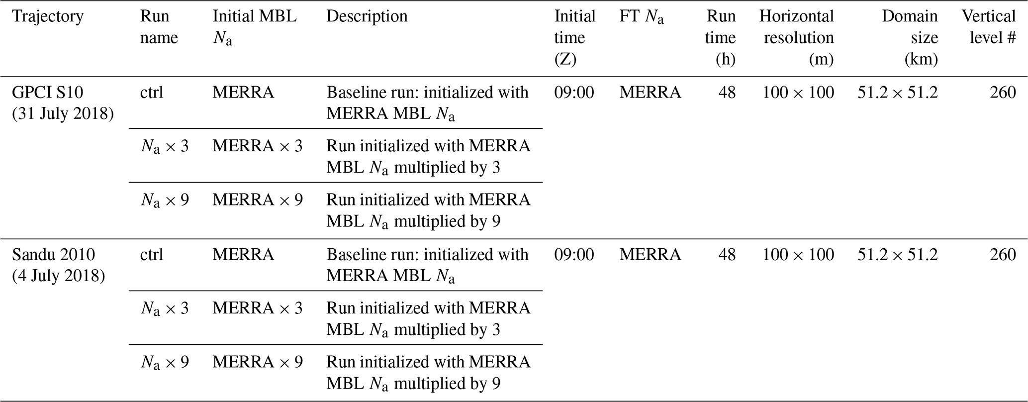
The PCA method selects 54 trajectories. From them, two cases are chosen, each from a different location and with distinct cloud and meteorological characteristics, as described later in Sect. 4. Table 2 summarizes the experiments in this study. The number of vertical levels in the model is 260, with the smallest vertical grid spacing being 7 m in the MBL top and Sc layer (from 450 to 1200 m). Above and below this vertical range, the vertical grid spacing gradually expands, such that it is 167 m just below the model top (which is at 4800 m) and is 20 m immediately above the ocean surface. The horizontal resolution is 100 m × 100 m, and the horizontal domain size is 51.2 km × 51.2 km.

Three runs are conducted for each trajectory: ctrl, N_a × 3, and N_a × 9. All three runs are initialized and forced in the FT with MERRA2 time-varying aerosol profiles. The ctrl run is initialized in the MBL with MERRA2 aerosol profiles. As in Erfani et al. (2022), to test for the sensitivity of cloud evolution to aerosols, the N_a × 3 and N_a × 9 runs are initialized with the MERRA2 MBL aerosol concentration multiplied by 3 and 9, respectively. Although the simulated FT N_a is nudged to the MERRA2 N_a throughout the simulation, the MBL N_a is prognosed freely for a natural simulation of aerosols, clouds, and precipitation. The time-varying vertical profiles of MERRA2 N_a are shown in Fig. 2 for two example trajectories and are derived from the mass mixing ratios of aerosol species following Appendix A in Erfani et al. (2022).

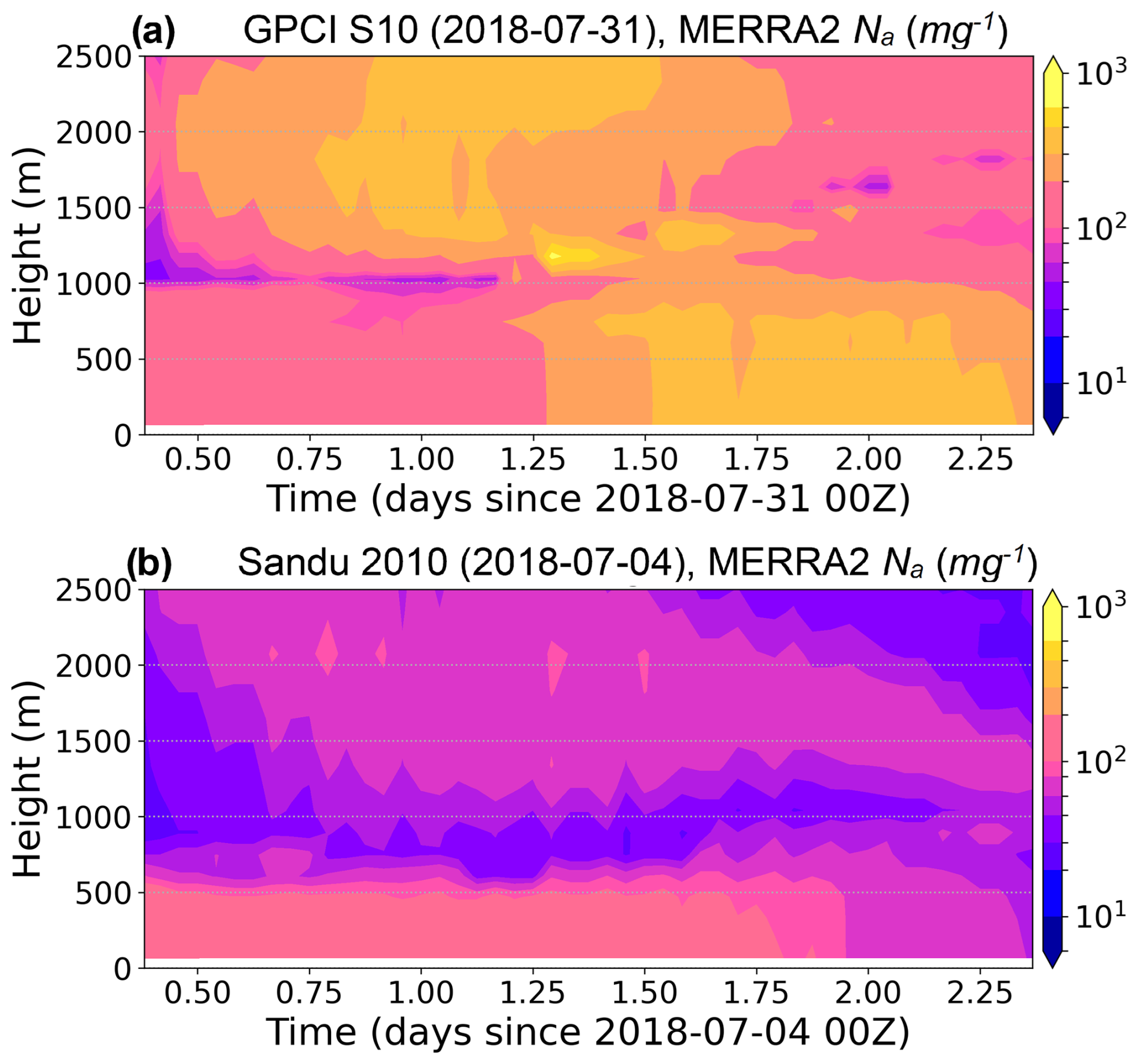
Figure 2 The time-height plot of MERRA2 N_a for the two trajectories used in this study for the LES case studies.

3 Statistical analysis

3.1 PCA results

One objective of using PCA in our study is to determine how the main modes of variation in key cloud properties are related to a select set of CCFs. This approach helps simplify the complex interactions between clouds and their environment by focusing on the most significant modes of variability and identifying the combinations of factors driving this variability. We first explore the R-values between various cloud properties and CCFs, as shown in Fig. S1. For instance, the R between CF and EIS is 0.31, which indicates a moderate positive relationship. In addition, the R between N_d and EIS is 0.36, which suggests that an increase in EIS is associated with an increase in N_d. Stronger stability near the inversion layer leads to weaker mixing, inhibiting the MBL from deepening, which ultimately enhances humidity and clouds near the top of the MBL (Klein et al., 2017; Wood and Bretherton, 2006). FT subsidence, represented by 700 hPa ω, is correlated with cloud properties (e.g., R between ω and CERES CTH is equal to −0.22, and R between ω and CF is equal to −0.13), showing that weaker FT subsidence leads to MBL deepening and increased cloudiness. Although it is intuitive to consider subsidence as promoting cloudiness, some studies (e.g., Klein et al., 2017; Myers and Norris, 2013) showed that, when controlling for EIS as well as subsidence, stronger subsidence results in decreased cloudiness. Surface WS is correlated with CTH, LWP, and precipitation, with the highest R-values corresponding to the changes in these properties along the trajectory: CERES ΔCTH (0.38), Δlog(SSMI LWP) (0.28), and Δlog(precip) (0.25). This is due to enhanced latent heat fluxes from the ocean surface that intensify latent heat release and facilitate cloud formation (Bretherton et al., 2013; Brueck et al., 2015). As explained in Sect. 2.3, absolute values of R greater than 0.14 are considered statistically significant, which provides confidence in the relationships seen between these variables.

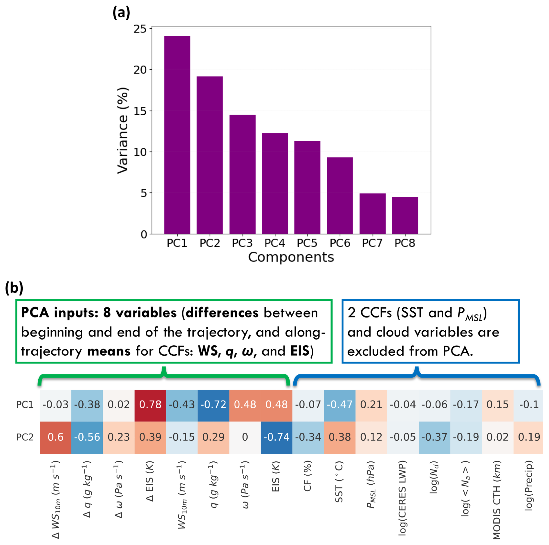
Figure 3 (a) The result of principal component analysis (PCA) showing the percentage of variance explained by each principal component (PC). (b) The relationship between the two PCs and key meteorological conditions and cloud properties are quantified through their correlation coefficient (R-value). The inputs to the PCA are presented as the first eight variables on the left; these are the differences between the beginning and end of the trajectory and the along-trajectory means for the cloud controlling factors (CCFs): WS, q, ω, and EIS.

Figure 3a illustrates the contribution of each PC to the total variance by showing the percentage of variance explained by each PC when PCA is conducted with eight variables as inputs. This visualization helps us to both understand the distribution of variance across the PCs and determine the number of PCs necessary to capture sufficient variability in our dataset. Because the PCs collectively encompass the entire variance in the dataset, the summation of the percentage of variance for all eight PCs amounts to 100 %. Notably, the first PC explains 24 % of the total variance, while the second PC explains an additional 19 %. Together, these two PCs account for a significant portion of the variability in the data. Thus, 43 % of the information regarding the variation in CCF properties is captured within PC1 and PC2, highlighting their importance in understanding cloud formation and evolution. Note that the contributions to the total variance differ among all the PCs, which shows different levels of importance among PCs.

In order to provide insight into which variables are most strongly associated with the modes of variation captured by PC1 and PC2, the R-values between each of the first two PCs and important CCFs, meteorological conditions, and cloud properties are shown in Fig. 3b. A more comprehensive set of R-values is provided in Fig. S1. For each PC, the R-values for the input variables (i.e., the first eight variables in each row) are associated with the eigenvector for that PC and determine the contribution of the input variable to that PC. This helps identify which CCFs are the most influential in the modes of variation represented by PC1 and PC2. The highest R with PC1 is for ΔEIS (0.78) and FT q (−0.72); i.e., the change in EIS along the trajectory and FT q are the most significant properties driving variability in PC1. For PC2, EIS and ΔWS are the most important variables, with R-values of −0.74 and 0.6, respectively, highlighting their roles in the mode of variation represented by PC2. Although SST is not an input to the PCA, it is correlated with both PC1 (−0.47) and PC2 (0.38), as SST is an input when computing EIS (Fig. S1). Additionally, PC1 and PC2 explain variations in some key cloud properties, as indicated by the fact that PC2 has R-values of −0.34 and −0.37 with CF and N_d, respectively, and PC1 has R-values of −0.28, −0.28, and −0.22 with CERES ΔCTH, Δlog(precip), and SSMI Δlog(LWP), respectively. This means that associations of the CCFs with cloud properties and their evolution along these Lagrangian trajectories are detected by PCA.

Focusing on PC1 and PC2 allows us to simplify the analysis while still capturing the most significant modes of variability. While PC3 explains an additional 14 % of the variability and is strongly correlated with Δω (R = −0.69) and ω (R = 0.53), variability in ω and Δω is partially captured by PC1 and PC2, respectively. We perform a linear regression of ω on PC1 and PC2 to find the best linear combination of $a\times \mathrm{PC}\mathrm{1}+b\times \mathrm{PC}\mathrm{2}$. The correlation between ω and this combination is 0.48. Similarly, the correlation between Δω and $c\times \mathrm{PC}\mathrm{1}+d\times \mathrm{PC}\mathrm{2}$ is 0.23. These values give the variance explained by the combination of the first two PCs for ω and Δω. In addition, including PC3 in further analysis would lead to a much larger number of representative trajectories, which is beyond our resources for conducting high-resolution, detailed LES in future work.

3.2 Phase space

To determine the full phase space of cloud variability in this region and identify a reduced number of trajectories that represent this range of variability, PC1 vs. PC2 is plotted for all qualifying trajectories (Fig. 4a). Additionally, and for each of the six select locations identified in Fig. 1a, nine trajectories are selected that represent the values of (−1.5σ, 0, 1.5σ) in the 2D PC1–PC2 plane (where σ is the standard deviation of each individual PC). This approach allows us to capture a representative sample of trajectories that encompass the range of variability in the PC phase space. As a result, the variability across 1663 trajectories can be sampled by just the 54 trajectories, shown with colored markers in Fig. 4a.

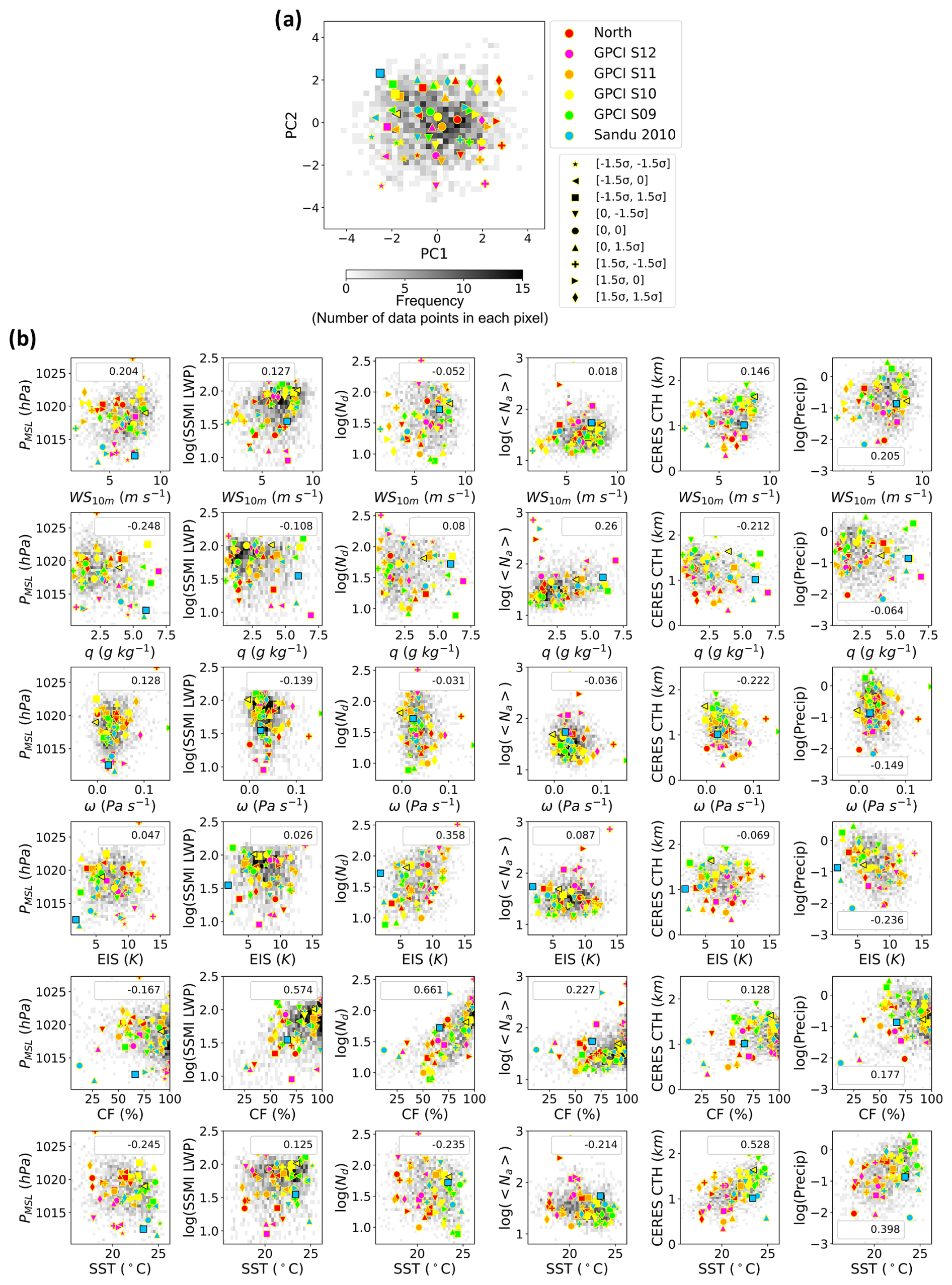
Figure 4 Phase space of variables. (a) Frequency plot of the first two principal components (PCs) for all qualifying trajectories used in the PCA. Here, each trajectory is represented as one data point. The gray shades show the frequency, i.e., the number of trajectories in each pixel. PCs associated with the six select locations shown in Fig. 1a are indicated by colored markers. For each location, different marker shapes are used to show nine trajectories that correspond to the standard deviation (−1.5σ, 0, 1.5σ) in this 2D space. (b) Each panel shows a frequency plot for pairs of cloud-controlling factors and cloud variables averaged along the trajectories, with their correlation coefficient shown in the box. The markers in each panel show the 54 points selected from the PC1–PC2 space mapped to the space for that pair of variables. In each panel, the two markers with a black edge show the two cases used for LES modeling in Sect. 4.

The selection of nine points for each initial location is intended to represent reasonable variations associated with each initial location, as 87 % of data points in a normal distribution fall within 1.5 standard deviations. It is noteworthy that the nine points for each initial location correspond to different parts of the PC plane, which hints at the distinct characteristics of each initial location. For instance, data points for the “North” initial location (see Fig. 1a) tend to be more frequent at larger values of PC1 and PC2, whereas the frequency of data points for “GPCI S12”, the closest initial location to the coast, is greater for lower values of PC1 and PC2. This shows that the PCA is sensitive to the geographical location of the trajectory origin, likely because the variability and co-variability of CCFs recognized by PCA occur in both space and time.

To assess the impact of reducing the number of trajectories from the full set on coverage of the range in the physical variables of interest, the data points in the PC1–PC2 plane are mapped to the corresponding CCFs and cloud properties, and, as in Fig. 4b, both the values for all trajectories (grayscale symbols) and for just the 54 select trajectories (colored symbols) are shown. Also as in Fig. 4b, for each pair of variables, the frequency of the along-trajectory averages in PC space is conveyed by the grayscale. Figure S2a shows the same but for the differences (change) in the CCFs and cloud properties between the beginning and end of the trajectories. This analysis summarizes the changes in variables over the course of the trajectories and their potential implications for cloud development.

While the distribution of data points varies significantly across the different phase planes in Fig. 4b, the 54 selected data points successfully represent much of the full spectrum of CCFs and cloud variables in each panel, indicating that this reduced set of trajectories effectively captures the key patterns and variations in the datasets. One limitation of our downsampling method is that it cannot represent the full variability of the dataset. We conduct a sensitivity analysis by randomly sampling trajectories for each location (Fig. S2b). This analysis reveals that while random sampling demonstrates some ability to capture variability, it provides a less representative subset of trajectories, especially within the extreme ranges of the datasets, compared to the PCA-based selection method. This highlights the capability of PCA in identifying trajectories that represent the variability in the dataset.

4 Numerical modeling

Here, we take two of the 54 selected trajectories identified as covering the range in cloud variability at our six representative sites in the NEP region and use them to demonstrate our approach to testing the LES-simulated cloud evolution against observed cloud evolution starting in the Sc region and moving toward the more Cu-dominated region. The two trajectories used for LES modeling were selected to illustrate distinct regimes among important cloud and atmospheric properties. In particular, as seen in Fig. 4b, the first case exhibits stronger surface pressure, higher LWP, higher CTH, lower FT q, stronger stability, and higher cloud coverage compared to the second case. In this way, and as explained throughout this section, these cases test the LES model under different combinations of CCFs and cloud properties. In a later study, this approach will be used to statistically analyze model performance across all 54 cases and, informed by this baseline of model performance, to systematically study the response of clouds to aerosol perturbations across all 54 cases.

4.1 First case: trajectory GPCI S10 (31 July 2018)

4.1.1 Observed characteristics

During the 2 d period of this trajectory, a permanent subtropical high-pressure system was located over the NEP, producing northeasterly surface winds in its southeastern flank and along the trajectory (Fig. 1b). Based on phase space analysis for satellite and reanalysis data (Fig. 4a), this case is characterized by an average PC2 value and a negative PC1 value. Among the 54 cases selected by PCA, and considering along-trajectory averages, it exhibits very strong 10 m WS, very weak ω, nearly overcast conditions (∼ 90 %), and strong LWP (Fig. 4b).

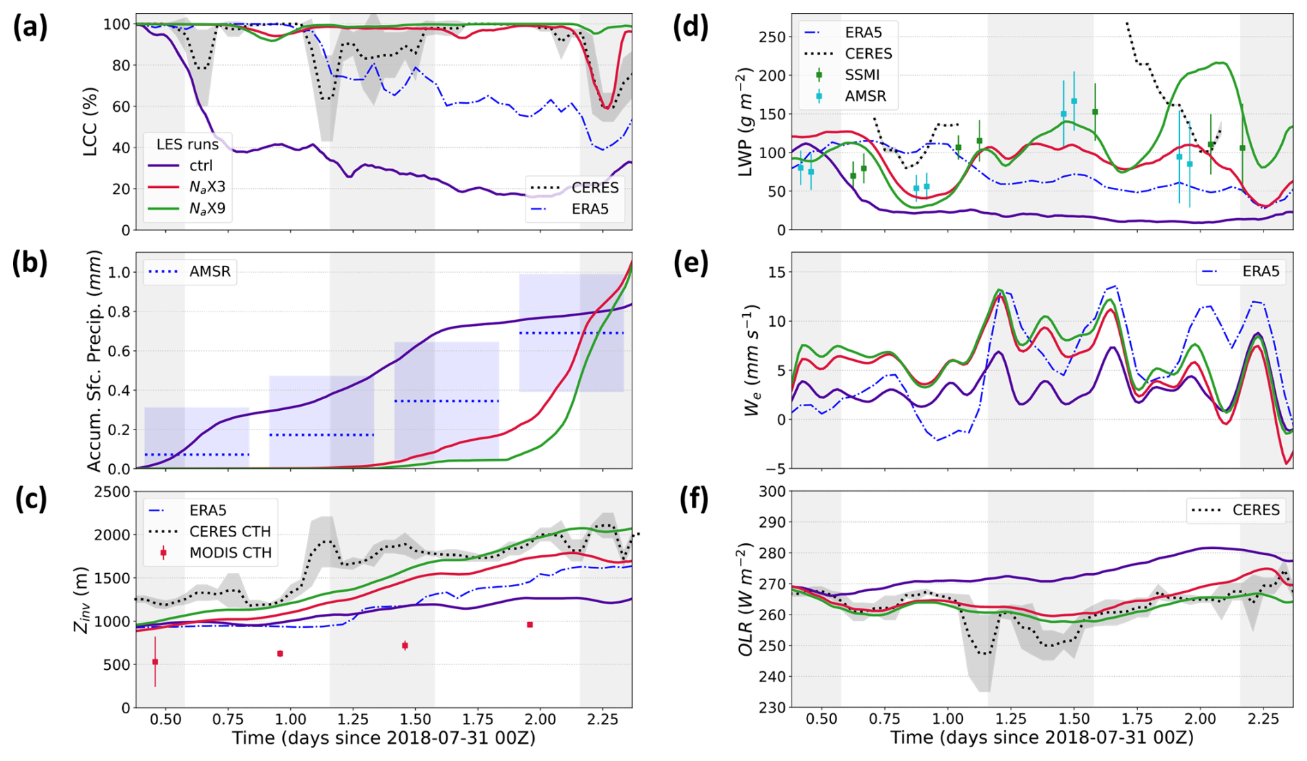
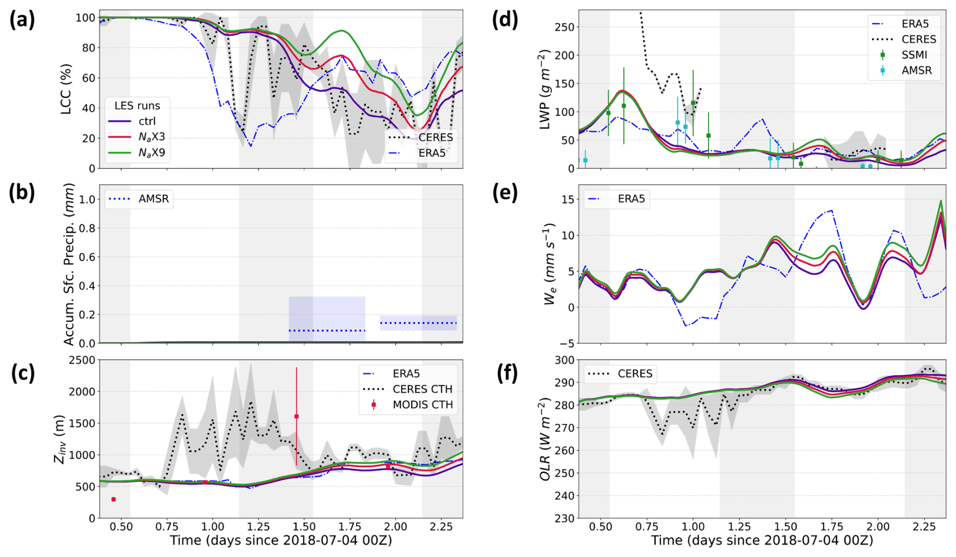
Figure 5 Time series of various observed and simulated domain-averaged meteorological variables for the GPCI S10 (31 July 2018) trajectory. (a) Low cloud cover (LCC), (b) accumulated surface precipitation, (c) inversion height (Z_inv), (d) liquid water path (LWP), (e) entrainment rate (w_e), and (f) outgoing longwave radiation (OLR). The nighttime periods are indicated with light-gray background shading.

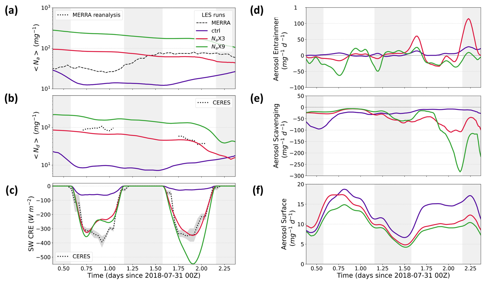
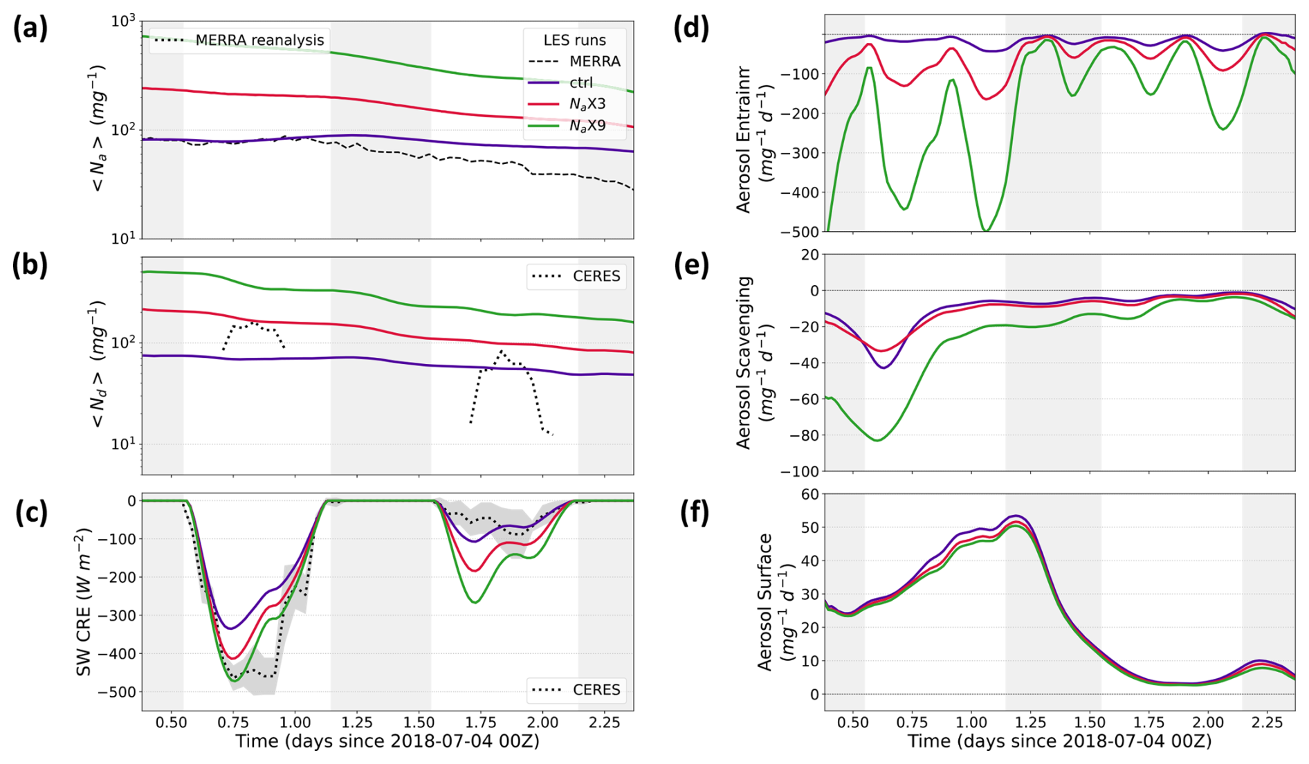
Figure 6 Time series of various observed and simulated domain-averaged variables for the GPCI S10 (31 July 2018) trajectory. (a) Total aerosol number concentration averaged within MBL (〈N_a〉), (b) cloud droplet number concentration averaged within MBL (〈N_d〉), (c) shortwave cloud radiative effect (SW CRE) at the top of atmosphere (TOA), (d) aerosol entrainment from the FT, (e) aerosol scavenging averaged within MBL, and (f) aerosol surface fluxes. The nighttime periods are indicated with light-gray background shading. CERES N_d values for zenith angles greater than 50° are excluded to avoid unrealistically low values at the start and end of each day.

Figures 5 and 6 show time series of various meteorological and aerosol properties along the trajectory from different observationally based datasets as well as from the LES runs. According to the CERES low cloud cover (LCC) retrievals (Fig. 5a), cloud breakup, defined as the reduction of domain-averaged LCC to 50 %, does not occur throughout the 48 h period, and overcast conditions prevail for the majority of the time. The ERA5 reanalysis LCC is lower than CERES LCC, as it gradually starts decreasing on the evening of the first day. A comprehensive comparison of MODIS and ERA5 cloud cover on a global scale and for the NEP region shows that ERA5 cloud cover is biased low (Wu et al., 2023). Considering that the CERES data are based on MODIS retrievals, it is justified to consider CERES, and not ERA5, as ground truth in this study. This case features moderate precipitation (Fig. 5b), with a slight enhancement of precipitation in the second half of the trajectory, consistent with a gradual increase in cloud droplet effective radius (r_e) from approximately 13 to 16 µm (Fig. S3b). The observed LWP consistently remains above 50 g m⁻², with the AMSR-retrieved LWP reaching 170 g m⁻² toward the end of the second night (Fig. 5d). The observed microwave products (AMSR and SSMI) agree quite well, but CERES LWP is larger than the microwave-retrieved LWP at almost all times. (Note that we discard CERES LWP, N_d, r_e, and cloud optical depth, or τ_c, when the zenith angle is greater than 70° to avoid erroneous values.) The ERA5 reanalysis LWP underestimates the observed LWP in the second half of the trajectory, associated with a consistent reduction in ERA5 LCC during this period.

The observed CERES and MODIS CTH and ERA5 Z_inv all show a gradual increase of approximately 500 m over the 48 h period (Fig. 5c); however, there are differences between datasets, with MODIS CTH being the lowest and CERES CTH being the highest. This discrepancy is present in some other trajectories and is worth further investigation in future studies. In this case, the CALIPSO Z_inv aligns more closely with ERA5 Z_inv (figure not shown).

The MBL-averaged total aerosol number concentration, 〈N_a〉, of about 30 mg⁻¹ from MERRA2 (Fig. 6a) indicates that the MBL is clean on the first day, but then 〈N_a〉 more than doubles during the night likely due to entrainment from an FT with high N_a (Fig. 2a). On the other hand, CERES N_d is around 100 mg⁻¹ on the first day and decreases to around 30 mg⁻¹ by the afternoon of the second day (Fig. 6b). This implies that MERRA2 〈N_a〉 is biased low (by approximately a factor of $\mathrm{1}/\mathrm{3}$) on the first day and is slightly biased high on the second day. Indeed, Erfani et al. (2022) showed that MERRA2 N_a is biased low for higher N_a values when compared to in situ measurements for 53 Lagrangian trajectories during the CSET campaign, and this highlights a limitation of MERRA2 reanalysis data in computing aerosol concentrations. Based on this, for future studies, we plan to initialize N_a within the MBL based on CERES N_d under the assumption that this N_a estimate will be less biased than the MERRA2 reanalysis in regions of overcast cloud. For this trajectory, the changes in cloud radiative properties from the decrease in N_d and the increase in LWP from the first day to the second day seem to cancel each other out, as the CERES-retrieved τ_c and the TOA shortwave cloud radiative effect (SW CRE) do not show significant day-to-day variations (Figs. S3a and 6c).

4.1.2 Reference run (N_a×3)

Because the run initialized with MERRA2 N_a within the MBL simulates early cloud breakup in contradiction to the observations, the N_a × 3 run is chosen as the reference simulation for this case study. Important cloud properties, particularly LCC, LWP, N_d, precipitation, SW CRE, and OLR, compare best to observed properties in the N_a × 3 run (Figs. 5 and 6). This highlights the ability of our LES to accurately simulate a range of cloud properties when it is initialized with N_a values that result in more accurate N_d, as the simulated 〈N_d〉 along the N_a × 3 run trajectory is quite similar to the CERES-retrieved N_d (Fig. 6b). Previous studies showed that N_d scales with N_a (Pringle et al., 2009; Svensmark et al., 2024). Both modeled and CERES-retrieved LCC broadly agree, though the N_a × 3 run is unable to simulate the timing and strength of two brief episodes of LCC reduction seen in the CERES retrievals on the first day and the following night (Fig. 5a). In the N_a × 3 run, any LCC reductions from the overcast conditions are associated with a remarkable decrease in LWP.

The N_a × 3 accumulated precipitation is always less than mean AMSR precipitation, except on the last night, but it generally stays within 1 standard deviation of observations (Fig. 5b). Precipitation onset occurs in the middle of the second night (much later than observations), enhances 12 h later, and continues until the end of the simulation. This likely causes the brief cloud reduction in the third night (Fig. 5a), along with the inhibition of Z_inv growth (Fig. 5c).

Z_inv in the N_a × 3 run and in ERA5 are initially equal due to the nudging in the startup stage, but Z_inv in the N_a × 3 run grows faster in the first half of the simulation and slower in the second half than in the ERA5 dataset, ultimately remaining very close to ERA5 Z_inv near the end of the run. This also explains the stronger entrainment rate (w_e) in the N_a × 3 run than in ERA5 in the first half of the simulation and vice versa in the second half (Fig. 5e) (note that w_e is estimated as the tendency of Z_inv relative to the W at the inversion level; Blossey et al., 2021; Erfani et al., 2022).

The gradual reduction in N_a and N_d is due to a general strengthening of the aerosol scavenging sink term (which is the sum of the accretion, autoconversion, and interstitial scavenging terms). The combined sink is stronger than the sum of the aerosol surface flux source term and entrainment from the FT (where the latter is a sink or source term depending on the total aerosol gradient between the FT and MBL) (Fig. 6d–f). In particular, the aerosol scavenging term is stronger in the second half of the simulation, leading to the onset of surface precipitation in the middle of the simulation. Although precipitation continues until the end of the run, the aerosol reduction and precipitation are not strong enough to cause SCT or cloud breakup, and Z_inv grows consistently until 6 h before the end of the simulation.

4.1.3 Impact of perturbed aerosols

The very low initial 〈N_a〉 (e.g., less than 30 mg⁻¹) in the ctrl run leads to early precipitation onset, which drives a rapid drop in N_a and N_d (Fig. 6a–b) and the occurrence of SCT (Fig. 5a) within the first 12 h of simulation. As defined by Erfani et al. (2022), an SCT occurs when LCC first falls below 50 % and remains below this threshold for at least 24 h or until the end of the simulation, whichever is shorter. This definition is designed to exclude LCC changes attributable solely to the diurnal cycle. This “precipitation-driven” type of SCT occurs quickly (e.g., less than 12 h) in LES experiments with a prognostic aerosol scheme due to the positive precipitation-aerosol feedback (Yamaguchi et al., 2017; Erfani et al., 2022). Consistent with the persistent precipitation, r_e remains greater than 15 µm (Fig. S3b). The aerosol scavenging sink term initially strengthens, leading to an extremely low N_d (less than 10 mg⁻¹), characteristic of vertically thin, horizontally extensive layers below the Z_inv, called ultra-clean layers (UCLs) (Wood et al., 2018). Note that this feature is not seen in the CERES observations. The time-height plots of N_d (figures not shown) indicate the simulation of UCLs near the inversion for the majority of the ctrl run time, but only for the last 8 h of the N_a × 3 run, because the ctrl run is initialized with a value of MERRA2 N_a that is 3 times smaller than CERES N_d.

As the simulation progresses further, the scavenging term gradually weakens. Combined with surface fluxes of aerosols and an entrainment source term for N_a (Fig. 6d–f), N_a and N_d are enhanced after the second night. Following the SCT, both LCC and LWP remain lower than 50 % and 50 g m⁻², respectively, causing low τ_c and a weak SW CRE (Figs. S3a and 6c). In addition, OLR is stronger in this run due to the greater longwave emission from warmer and shallower cloud tops (as seen in Z_inv) and from a warmer surface, as LCC is below 40 % most of the time. MBL deepening is suppressed in this clean and precipitating environment. Two mechanisms have been proposed to explain this: (1) low aerosol concentrations correspond to weak turbulence, a decoupled MBL, and reduced entrainment (Sandu et al., 2008); and (2) precipitation depletes LWP from the inversion layer, resulting in decreased entrainment (Blossey et al., 2013).

Although the ctrl and N_a × 3 runs are very distinct, the N_a × 3 and N_a × 9 runs have quite similar cloud properties in the first half of simulations. The N_a × 9 entrainment rate is stronger than that of N_a × 3 during the first and second nights likely due to enhanced entrainment associated with N_d  increases in non-precipitating clouds (e.g., Igel, 2024) (see Figs. 5e, 6b). While this leads to somewhat smaller LWP during the first day of the simulation than in N_a × 3, the larger N_d in the N_a × 9 run leads to the delayed initiation of aerosol scavenging and precipitation (Fig. 6b, e). The Twomey effect (Platnick and Twomey, 1994) is visible in comparisons of SW CRE (Fig. 6c), where the increased N_d in the N_a × 9 run leads to a stronger SW CRE (Fig. 6c) than N_a × 3 during the first daytime despite the N_a × 9 run having similar LCC (Fig. 5a) and smaller LWP (Fig. 5d). Later, precipitation plays a more important role in modulating aerosol impacts: compared to the N_a × 3 run, the delayed onset of precipitation in the N_a × 9 run is followed by more MBL deepening (Fig. 5c) and larger LWP, τ_c, and SW CRE differences between the two runs in the second half of the simulation. LCC also never drops below 90 % in this high-N_a run.

Unlike the two other runs, entrainment from the FT drives the decreases in N_a on average in the N_a × 9 run (Fig. 6d), as the MBL N_a is so high that it reverses the MBL-FT aerosol gradient. Additionally, the scavenging term is a stronger sink toward the end of this run (Fig. 6e), driving a decrease in N_a that leads to a sudden enhancement of precipitation.

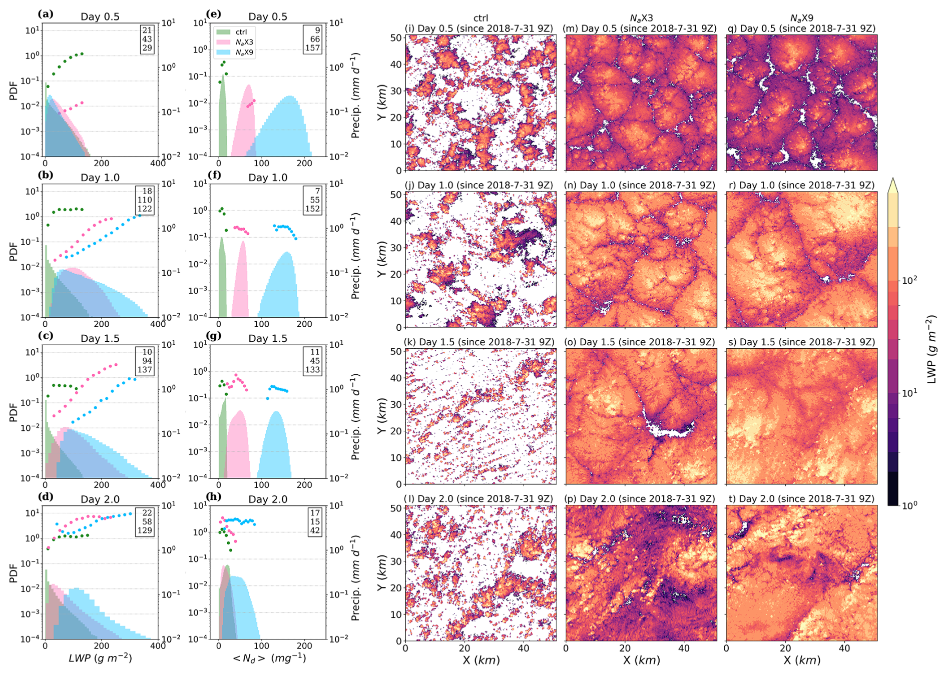
Figure 7 Probability distribution functions of LWP (a–d) and 〈N_d〉 (e–h) at four instantaneous times for three LES experiments (ctrl, N_a × 3, and N_a × 9) along the GPCI S10 (31 July 2018) trajectory. The markers present precipitation in bins of the variable on the x axis, and the numbers within the box in each panel show the mean value of the variable given on the x axis for that specific time (from top to bottom for ctrl, N_a × 3, and N_a × 9, respectively). (i–t) Cloud morphology showing LWP at four times for three LES runs.

The cloud morphology, shown in 2D maps of LWP for the N_a × 3 run (Fig. 7m–p), demonstrates the development of the mesoscale organization in the form of closed cells within the Sc clouds early on, with the mesoscale cell size and cloud LWP increasing with time. The probability distribution functions (PDFs) of LWP and N_d (Fig. 7a–h) show that precipitation is more frequent in regions of high LWP and low-to-moderate N_d.

The morphology and PDF plots in Fig. 7 also demonstrate the impact of the initial aerosol concentration on cloud field development. Due to the clean environment and early SCT in the ctrl run, scattered Cu clouds form 12 h after the initial time and are maintained throughout the simulation (Fig. 7i–l), with not much change in the cloud LWP and N_d frequency distributions and the precipitation within the Cu cores (Fig. 7a–h). The cloud morphology for the N_a × 9 run is similar to that for the N_a × 3 run 12 h after the initial time, but the N_a × 9 mesoscale cell size and LWP increase more rapidly. The increase in mesoscale cell size for the N_a × 9 run is likely due to enhanced aerosol entrainment and suppressed precipitation. For more details, the reader is referred to Sect. 4.2.3. The PDFs illustrate a broader LWP spectrum with a higher probability of larger LWP in the N_a × 9 run compared with the N_a × 3 run 24 h after the initial time until the end of the run (Fig. 7b–d). This spectrum broadening is associated with the precipitation onset in larger LWP bins and faster aerosol removal from the MBL (Fig. 7e–h), which ultimately leads to more intense precipitation toward the end of the N_a × 9 run compared to the N_a × 3 run (Fig. 5b). Also, the r_e value during the precipitation onset for the N_a × 9 run is approximately 9 µm, which is smaller than for the N_a × 3 run (∼ 12 µm) and the ctrl run (∼ 15 µm) (Fig. S3b). As explained by Wood et al. (2009), precipitation can initiate with a smaller r_e for larger N_d and LWP.

4.2 Second case: trajectory Sandu 2010 (4 July 2018)

4.2.1 Observed characteristics

For our second case, in addition to the permanent subtropical high over the NEP, a tropical cyclone developed to the east, visible in the surface wind pattern (Fig. 1c) and confirmed by satellite imagery and a humid FT. This is seen in the time-height plot of q_t along the trajectory (figures not shown), which is located between the southeast edge of the high and the northwest edge of the cyclone. The phase space analysis (Fig. 4a) shows that this case has the highest PC2 values and one of the lowest PC1 values among the 54 selected cases. Based on along-trajectory averages of physical variables (Fig. 4b), this case is characterized by very low P_MSL, very weak stability (lowest EIS), and high 700 hPa q.

Figure 8 Same as in Fig. 5 but for the Sandu 2010 (4 July 2018) trajectory.

CERES LCC (Fig. 8a) shows a brief cloud breakup at the end of the first day and a major breakup starting in the early morning of the second day that lasts until the third night, with cloud cover restoring a few hours before the end of the run. According to the previously mentioned SCT definition, this does not qualify as SCT; however, others (e.g., Sandu and Stevens, 2011; Baró Pérez et al., 2024) simply define SCT as the first time LCC falls below 50 %. In addition, this cloud breakup initiates during the dark hours, suggesting it might not be due to the diurnal cycle. Nevertheless, we use the term “cloud breakup” for this case throughout this study. ERA5 LCC appears out of phase with that from CERES, showing cloud breakup at the end of the first day and cloud restoration on the morning of the second day.

AMSR observations indicate that precipitation is extremely weak in this case, with accumulated precipitation of approximately 0.1 mm after 2 d. Precipitation onset occurs on the second night before the major cloud breakup; however, CERES r_e (Fig. S4b) does not show a significant day-to-day change and remains below 15 µm, fluctuating between 10 and 13 µm in the middle of the days. The microwave (SSMI and AMSR) LWP increases during the first 6 h of the simulation and then decreases until the second day (Fig. 8d). The LWP from all three observational products falls below 50 g m⁻² during the cloud breakup. Similar to the first case, the CERES LWP is generally greater than the microwave LWP, but the two microwave retrievals, from AMSR and SSMI, remain similar. CERES CTH and, to some extent, MODIS CTH show an unusual deepening from the middle of the first day until the end of the following night (Fig. 8c). This seems to be due to the presence of upper-level ice clouds, also evident in the low values of OLR during this period. Otherwise, CERES and MODIS CTH and ERA5 Z_inv generally agree, showing an enhancement of 200–500 m from the start to the end of the trajectory. Based on ERA5 Z_inv, this increase begins on the second night before the cloud breakup but slows down on the second day. This is associated with the decoupling of the MBL, evident from the time-height plot of ERA5 q_t, where the q_t difference between the lower and upper MBL increases along the trajectory (figure not shown).

Figure 9 Same as in Fig. 6 but for the Sandu 2010 (4 July 2018) trajectory.

The initial value of the MERRA2 〈N_a〉 for this trajectory is 70 mg⁻¹; then, 〈N_a〉 gradually decreases starting on the second night to around 30 mg⁻¹ by the end of the trajectory (Fig. 9a). Consistent with this, CERES N_d decreases from the first day to the second day (Fig. 9b). However, as in our other trajectory, the MERRA2 〈N_a〉 around solar noon is significantly smaller (here, by a factor of 2) than the CERES N_d, which is clearly not physically consistent. Again, this suggests that simulations initialized with MERRA2 〈N_a〉 may struggle to match CERES N_d, so other options for aerosol initialization in the MBL should be considered. Note that for this trajectory, both 〈N_a〉 and 〈N_d〉 values are significantly higher than the 10 mg⁻¹ threshold used by Wood et al. (2018) to identify a UCL.

CERES τ_c decreases significantly over the trajectory, from an average of 15 on the first day to an average of 3 on the second day (Fig. S4a), consistent with the reduction in both N_d and LWP. Additionally, the SW CRE from CERES demonstrates an approximately 5-fold decrease from the first to the second day (Fig. 9c) due to cloud breakup and τ_c reduction.

4.2.2 Reference run (ctrl)

For this case, the ctrl run serves as our reference simulation because it performs better at simulating most variables, such as LCC, N_a, N_d, and SW CRE, compared to the perturbed runs (Figs. 8 and 9). This improved performance relative to the first case study likely results from the thinner clouds with smaller LWP in this case study, which do not precipitate significantly, even when initialized with the MERRA N_a that are biased low relative to CERES N_d (Fig. 9a–b), but not by as much as for our first case. The noisy patterns seen in most observed variables are absent in the ctrl run, likely due to slow FT nudging. While the ctrl run does not capture the first, brief observed cloud breakup, it accurately simulates the timing and rate of the second cloud breakup on day two and the cloud restoration on the last night (Fig. 8a). The ctrl run successfully simulates the microwave LWP pattern, showing enhancement during the first 6 h followed by a reduction. However, the timing of LWP reduction is earlier than microwave observations by a few hours (Fig. 8d). Despite this, the ctrl run LWP remains within the lowest bound of the microwave LWP or very close to it during this period and is mostly close to the mean microwave LWP at other times. Unlike the AMSR-retrieved precipitation, the ctrl run simulates no precipitation, indicating that the cloud breakup in the model is not precipitation-driven. Instead, it appears to be affected by the MBL deepening (Fig. 8c), which enhances w_e during the second night (Fig. 8e). This is indicative of the deepening-warming cloud breakup mechanism, driven by the deepening and decoupling of the MBL (Bretherton and Wyant, 1997; Wyant et al., 1997) and enhancement of entrainment near the inversion (Ackerman et al., 2004). This type of cloud breakup occurs at a much slower rate compared to precipitation-driven cloud breakup, as shown by the ctrl run for the first case (Fig. 5) and by precipitating runs in Erfani et al. (2022).

A precipitation-driven SCT is very unlikely for this case, as an environment with N_d higher than 30 mg⁻¹ and LWP lower than 30 g m⁻² is associated with precipitation of less than 0.03 mm d⁻¹ (Fig. A3 in Wood et al., 2009). The increase in w_e in the ctrl run before the cloud breakup during the second night is consistent with that seen in the ERA5 w_e, though ERA5 shows a stronger increase in w_e (Fig. 8e). This period is followed by a reduction in w_e that lasts until the middle of the second day. The MBL deepening on the second night is not seen in the CERES retrievals due to the presence of ice clouds during the first day. When ice clouds are absent, the ctrl run Z_inv and OLR agree well with that from the CERES retrievals (Fig. 8c and f).

The ctrl run underestimates the magnitude of the observed SW CRE on the first day (Fig. 9c), despite having overcast conditions in both the ctrl run and the CERES retrievals. This appears to be due to an underestimation of τ_c during this time (Fig. S4a), which is the result of low LWP and N_d in the ctrl run (Fig. 9a), which are lower than the CERES values during the first day. The ctrl run agrees well with CERES values of τ_c and SW CRE during the second day.

Although the ctrl run simulates the general trend in MERRA2 N_a and CERES N_d (e.g., an overall reduction in 〈N_a〉 and 〈N_d〉 from the start to the end of the run, particularly in the second half of the simulation), the rate of 〈N_a〉 reduction is slower than that in MERRA2 (Fig. 9a, b). Specifically, the ctrl run 〈N_a〉 decreases from 80 to 60 mg⁻¹ (Fig. 9a), and the ctrl run 〈N_d〉 decreases from 70 to 50 mg⁻¹ (Fig. 9b). Based on the time-height plots of N_a and N_d (not shown), their values tend to be lower near the inversion but do not drop below 20 mg⁻¹; therefore, these reductions are insufficient to develop UCLs. It seems that 〈N_a〉 is relaxing toward the FT values, which are below 50 mg⁻¹ near the inversion. During the first half of the simulation, both the aerosol scavenging sink term and the aerosol surface flux source term are stronger, while the aerosol entrainment term remains a sink term throughout the run (Fig. 9d–f). The balance among these three terms results in negligible changes in 〈N_a〉 and 〈N_d〉 during the first half of the simulation, followed by a gradual reduction in the second half. Overall, the moderate initial aerosol concentrations and their slow reduction prevent the formation of large cloud droplets (as indicated by r_e, which remains within 8–12 µm throughout the run and is slightly smaller than CERES values; Fig. S4b) and the initiation of precipitation (Fig. 8b).

4.2.3 Impact of perturbed aerosols

Compared to the ctrl run, the N_a × 3 run's higher 〈N_a〉 and 〈N_d〉 during the initial hours (Fig. 9a–b) lead to a stronger FT-MBL aerosol gradient. This results in a stronger aerosol entrainment sink term (Fig. 9d), causing a more pronounced decrease in both 〈N_a〉 and 〈N_d〉 over the trajectory duration. Despite this, 〈N_a〉 and 〈N_d〉 in the N_a × 3 run remain at least twice those in the ctrl run. Cloud breakup in the N_a × 3 run occurs a few hours later than in the ctrl run, with LCC in the N_a × 3 run remaining 15 %–20 % higher than in the ctrl run during the second day. This delayed cloud breakup corresponds to a slightly stronger deepening of the MBL (approximately 100 m; Fig. 8c) and, consequently, a slightly stronger w_e (Fig. 8e) and lower OLR (Fig. 8f) compared to the ctrl. These results align with Sandu et al. (2008), which demonstrated that enhanced entrainment in cases with high N_a leads to stronger turbulence and MBL deepening; however, this impact is modest for this second case study.

During the first 12 h of simulation, the higher τ_c in the N_a × 3 run, compared to the ctrl run (Fig. S4a), can be attributed to the elevated initial 〈N_d〉, as the initial LWP is very similar between the two runs. This corresponds with a reduction in r_e by 2–3 µm in the N_a × 3 run, compared to the ctrl run, primarily due to the Twomey effect during the first day, given that LCC and LWP remain relatively unchanged between the runs. Also, the change in τ_c explains the stronger SW CRE in the N_a × 3 run during the first day. On the second day, however, the stronger SW CRE in the N_a × 3 run is more influenced by the higher LCC in this run (Fig. 8a) and less by τ_c. In other words, the role of CF adjustment in SW CRE differences between the runs becomes important on the second day, as evidenced by the differences in LCC.

The run with very high N_a, N_a × 9, simulates strong aerosol entrainment and scavenging sink terms (Fig. 9d–e), leading to a faster reduction in N_a and N_d compared to the N_a × 3 run (Fig. 9a–b). The cloud breakup in the N_a × 9 run is delayed by a few hours (Fig. 8a), associated with slightly greater MBL deepening, enhanced entrainment, and reduced OLR, compared to the N_a × 3 run (Fig. 8c, e, f). The higher aerosol concentration in the N_a × 9 run leads to smaller r_e (Fig. S4b), higher τ_c (Fig. S4a), and an increased magnitude of SW CRE (Fig. 9c). The change in SW CRE from the ctrl to the N_a × 3 run is stronger than from the N_a × 3 to the N_a × 9 run during the first day. Considering the similar overcast conditions and LWP values across all three runs, this highlights the dominance of the Twomey effect and albedo susceptibility. This impact diminishes on the second day as CF adjustment becomes more significant.

Maps of LWP for the ctrl run (Fig. S5i–l) show the formation of overcast Sc clouds and mesoscale organization 12 h after the initial time, which then develop into closed cells later on. The dissipation of Sc clouds and cloud breakup are demonstrated by scattered Cu clouds 36 h after the initial time, but their frequency and size increase toward the end of the simulation due to cloud restoration. The PDFs of LWP (Fig. S5a–d) indicate that although the mean and median LWP values show a general decrease over time until near the end of the runs, the LWP spectrum broadens with a higher probability of larger LWP, suggesting enhanced LWP in the cores of mesoscale cells over time. The evolution of cloud morphology and LWP PDF for the N_a × 3 and N_a × 9 runs is similar to that for the ctrl run, but higher MBL aerosols lead to larger mesoscale cell sizes (Fig. S5o, p, s, t) with more water in their cores, as evident from the broadening of the LWP spectrum toward the larger values (Fig. S5c–d).

For each run and at each time, the average length scale of mesoscale cells is quantified in Fig. S6 as the wavelength below which $\mathrm{2}/\mathrm{3}$ of the LWP variance is contained following the methodology of de Roode et al. (2004) (see their Fig. 2). During the overcast Sc regime on day 0.5, the LWP PDF (Fig. S5a) shifts toward smaller values with increased N_a, as expected from the sedimentation-entrainment feedback (Ackerman et al., 2004), and domain-averaged LWP decreases with increasing N_a, while the length scale of mesoscale cells is larger in the N_a × 3 and N_a × 9 runs than in the ctrl run (Fig. S6a). Later on (days 1.5 and 2.0), when cloud breakup occurs and Cu clouds emerge, both mean LWP and cell size values are larger in the N_a × 3 and N_a × 9 runs than in the ctrl run. Therefore, the reduced LWP due to aerosol perturbations in the non-precipitating boundary layer at the beginning of the runs appears to be a short-lived effect in our study, as the opposite occurs when Cu under Sc becomes dominant. The influence of N_a on mesoscale cell size is not well understood. Zhou and Feingold (2023) highlighted the relationship between cell size and N_d, but their study focused on how cell size regulates N_d and LWP rather than aerosol impact on the cell size. Further research is required to investigate the mechanisms behind the dependence of cell size on N_a.

Turbulence is slightly stronger in the N_a × 9 run than that in the other two runs before the cloud breakup and at the very end of the run (figure not shown). Stronger turbulence might help bring more moisture to the cloud layer, hence higher LWP in the Cu cores in the N_a × 9 run. Note that this case has extremely weak precipitation, with precipitation in all three runs (Fig. S5a–h) being 2 or more orders of magnitude smaller than for the first case. Therefore, the impact of precipitation on turbulence is negligible.

5 Discussion

The PCA approach demonstrated in this study has been particularly effective in identifying a subset of Lagrangian trajectories that not only represent the variability within the PC space but also span the full range of key cloud properties. This highlights the potential of PCA for refining complex datasets while preserving critical physical characteristics relevant to ACI and MCB studies.

An important challenge is defining a ground truth against which models could be validated, due to the considerable variability observed in cloud property datasets from reanalysis and satellite retrieval products. This variability underscores the complexities and uncertainties inherent in both products, which might affect confidence in the results. In addition, the relatively coarse spatial resolution of these products, compared to the LES resolution, could undermine the representation of diverse aerosol and cloud properties.

In general, satellite retrievals are more reliable than reanalysis products for Sc clouds. Based on climatological averages for the NEP region, ERA5 LCC is biased low when compared to MODIS (Wu et al., 2023), and because CERES LCC is based on MODIS retrievals, CERES is more robust than ERA5 when studying LCC. Microwave (AMSR and SSMI) retrievals of LWP are reliable for Sc clouds because they compare well with in situ measurements (Painemal et al., 2016). The Z_inv values calculated in our study based on vertical profiles of ERA5 T and q_t appear to be more robust than other products. The CTH from MODIS retrievals is created based on data stratified within bins of T each having a range of 5 °C; as such, it might not be accurate for individual cases, but it performs well on average (Eastman et al., 2017).

Over the NEP and at higher values of N_a, MERRA2 N_a is biased low when compared to in situ measurements (Erfani et al., 2022). In the future, a critical step in forcing and initializing our LES with MBL aerosols will be to base aerosol concentrations on a combination of multiple observational (e.g., CERESN_d) and reanalysis (e.g., MERRA2 N_a) datasets, rather than using MERRA2 alone, to ensure more reliable simulations of ACIs. Given that MERRA2 N_a is simulated by assimilating MODIS aerosol optical depth (which represents the optical property of aerosols throughout the column of troposphere), it can be inaccurate at certain levels and locations and is often subject to sudden changes associated with the aerosol optical depth data assimilation. Further research is required to achieve a more accurate N_a dataset on a global scale and for a long period of time. Assimilating satellite products with higher temporal resolution (e.g., Geostationary Operational Environmental Satellite, or GOES) or incorporating satellites with vertical profile information (e.g., CALIPSO) could improve the accuracy of such datasets in the future. For now, CERES provides satellite estimates of N_d in the cloud layer, so it likely reflects N_a more accurately in these Sc clouds. These estimates also result in N_a values that are more consistent with other CERES products, such as TOA radiative fluxes, which are considered the most accurate measurements (Su et al., 2015).

Given the absence of N_a observations away from aircraft campaigns, significant uncertainty exists in our initial N_a and will lead to uncertainty in the response of these cases to perturbed aerosols. When the initial N_a is erroneous, we expect biased responses to aerosol perturbations, with stronger biases for precipitating clouds and weaker biases for non-precipitating clouds, as suggested by previous studies (e.g., Chun et al., 2023). However, because the LWP, LCC, and SW CRE of our unperturbed simulations depend both directly and indirectly on the initial N_a, the agreement of these quantities with observations suggests that our initial N_a is consistent with observations, within the limitations of our model. The GPCI S10 case exemplifies this, as comparisons indicate that MERRA N_a is inconsistent with both observations and our model framework. While such an internal consistency check between unperturbed simulations and observations does not guarantee that the initial N_a is correct, it strengthens confidence in our predicted responses to aerosol perturbations relative to a case without such a check.

6 Summary

The objective of this study is to develop an approach for selecting and analyzing a representative set of cases for studying LES model performance and how ACIs and MCB affect key cloud properties in the absence of in situ observations. Utilizing ECMWF ERA5 wind data, we generate 2208 Lagrangian isobaric (950 hPa) MBL forward trajectories initialized at six locations within the subtropical NEP during JJA 2018–2021. Eliminating trajectories that pass near or over land or that include ice clouds reduces this to 1663 trajectories. Note that we retain cases with limited amounts of ice cloud to avoid selection bias for the low cloud cases. Meteorological, cloud, aerosol, and radiation variables from reanalysis and satellite data are compiled along these trajectories to create a library of Lagrangian observations. We then use a selected number of CCFs (e.g., along-trajectory means and differences between the beginning and end of each trajectory for WS, q, ω, and EIS) and conduct PCA to reduce the data dimensionality. Based on the PCA results, we find that two PCs capture 43 % of the variability in the CCFs. To span the meteorological diversity of the dataset, nine trajectories are selected for each of the six initial locations in our study region, where the nine trajectories correspond to the values of (−1.5σ, 0, 1.5σ) in the PC1–PC2 plane. This reduces the total of 1663 trajectories to a subset of 54 trajectories that span most of the variation in the CCFs, aerosol concentrations, and cloud properties relevant to their evolving radiative effect.

Some previous studies have employed aircraft measurements from intensive observational field campaigns to initialize and force Lagrangian LES runs (Blossey et al., 2021; Erfani et al., 2022). Because in situ measurements are rare over the remote oceans, here we develop a methodology for doing routine LES modeling that is initialized with and tested against satellite retrievals and reanalysis data. In addition to meteorological data, the LES is forced with an accumulation-mode aerosol N_a calculated from the MERRA2 masses of aerosol species and their assumed particle size distributions, applying the technique described in Erfani et al. (2022) to convert aerosol mass to number concentrations. In addition, a thermodynamic “profile sharpening” method is developed to modify the initial T and q_t vertical profiles from ERA5 in an approach that results in cloud LWP matching that from the microwave-instrument satellite retrievals. This method leads to the instantaneous formation of a well-mixed stratiform-topped MBL in the LES.

The LES used in this study is SAM (Khairoutdinov and Randall, 2003) coupled with a prognostic aerosol scheme (Berner et al., 2013) that accounts for aerosol budget tendencies such as coalescence and interstitial scavenging, surface sources, and entrainment from the FT. From 54 Lagrangian cases, two cases are selected as examples to conduct 2 d high-resolution, large-domain Lagrangian LES experiments in order to simulate cloud evolution under observed as well as perturbed aerosol conditions. The results of a few runs for the two cases reveal that our LES is capable of simulating observed conditions when initialized with realistic aerosol and meteorological conditions. The first case is precipitating, which implies a potential for a precipitation-driven cloud breakup if the environment is clean. Enhancing the initial aerosol concentration among different runs increases N_d, reduces r_e, enhances cloud albedo, suppresses precipitation, and increases TOA SW CRE, in agreement with previous studies (Sandu and Stevens, 2011; Yamaguchi et al., 2017; Christensen et al., 2020; Blossey et al., 2021). $\mathrm{d}\left(\mathrm{SW}\mathrm{CRE}\right)/\mathrm{d}(N_{\mathrm{d}}$) is nonlinear, with a larger magnitude increase (more cooling) from the ctrl run to the N_a × 3 run than from the N_a × 3 run to the N_a × 9 run. This seems to be due to the positive precipitation-aerosol feedback for the ctrl run, which quickly dissipates the clouds.

The second case is non-precipitating, and the classic deepening-warming cloud breakup happens in both the control and increased-aerosol runs. More MBL aerosol leads to stronger entrainment, more delayed cloud breakup, and a stronger SW CRE. This type of SCT was simulated in previous studies (Baró Pérez et al., 2024; Diamond et al., 2022) and seems to be more common in a polluted environment. Compared to the first case, cloud breakup occurs at a slower rate, and perturbed aerosols among different runs have a smaller impact on SW CRE and cloud breakup due to the absence of a precipitation-aerosol feedback.

The simulations in this study demonstrate that reanalysis meteorological and aerosol data can be used for initializing and bounding LES runs to produce realistic baseline simulations of low marine cloud fields in the absence of aircraft field campaigns. In the future, we will conduct LES experiments for a large number of Lagrangian cases from PCA results. This will enable us to synthesize valuable statistics to assess how well LES can simulate the cloud life cycle under the “best estimate” environmental conditions and how sensitive the simulated clouds are to variations in these driving fields. This procedure will contribute to advancing our understanding of intentional MCB efficacy under a range of representative conditions.

Appendix A: Sharpening procedure of thermodynamic profiles

This procedure utilizes satellite microwave retrievals of LWP to sharpen reanalysis (particularly ERA5) temperature and moisture vertical profiles through an optimization technique at a specific time near the inversion level.

A1 Preparing variables

We use a number of reanalysis and satellite variables to sharpen the ERA5 temperature and moisture profiles near the inversion level. At each time (generally the time corresponding to when we initialize an LES run), the vertical profiles of ERA5 normalized liquid water static energy (T_l) and the total water mixing ratio (q_t) are calculated as:

$$\begin{array}{}\text{(A1)}& {\displaystyle }{T}_{\mathrm{l}}=T+g{\displaystyle \frac{z}{C_p}}-q_{\mathrm{l}}{\displaystyle \frac{L_{\mathrm{v}}}{C_p}},\text{(A2)}& {\displaystyle }{q}_{\mathrm{t}}=q_{\mathrm{v}}+q_{\mathrm{l}},\end{array}$$

where T is temperature, q_v is the water vapor mixing ratio, q_l is the cloud liquid water mixing ratio, z is height, g is Earth's gravitational acceleration, C_p is the specific heat of dry air at constant pressure, and L_v is the latent heat of vaporization. We conduct separate calculations for the MBL and lower FT, but first we need to calculate the inversion height (Z_inv), which is defined as the height where $\left(\frac{\mathrm{d}{\mathit{\theta }}_{\mathrm{l}}}{\mathrm{d}z}\right)\left(\frac{\mathrm{dRH}}{\mathrm{d}z}\right)$ is minimized over the atmospheric column at each time and location (Blossey et al., 2021; Erfani et al., 2022). RH is relative humidity, and θ_l is liquid water potential temperature.

First, the lower FT profile sharpening method is explained. We assume that L_FT is a height above the inversion where the ERA base profiles feel no impact from the MBL. This is selected to be 500 m. Therefore, for z > Z_inv+L_FT:

$$\begin{array}{}\text{(A3)}& {\displaystyle }{T}_{{\mathrm{l}}_{\mathrm{shrp}}}=T_{{\mathrm{l}}_{\mathrm{base}}},\text{(A4)}& {\displaystyle }{q}_{{\mathrm{t}}_{\mathrm{shrp}}}=q_{{\mathrm{t}}_{\mathrm{base}}},\end{array}$$

where the subscript “shrp” refers to sharpened profiles and the subscript “base” to the baseline profiles. For Z_inv < z < Z_inv+L_FT, a line is fitted to the $T_{{\mathrm{l}}_{\mathrm{base}}}$ and $q_{{\mathrm{t}}_{\mathrm{base}}}$ profiles away from the inversion (e.g., Z_inv+L_FT < z < Z_inv+3L_FT) and is extrapolated down to the inversion.

Now, the MBL profile sharpening method is described. At the top of the MBL (z=Z_inv), the values are calculated as:

$$\begin{array}{}\text{(A5)}& {\displaystyle }{T}_{{\mathrm{l}}_{\mathrm{shrp}}}=T_{{\mathrm{l}}_{\mathrm{base}}}+\mathrm{\Delta }{T}_{{\mathrm{l}}_{\mathrm{inv}}},\text{(A6)}& {\displaystyle }{q}_{{\mathrm{t}}_{\mathrm{shrp}}}=q_{{\mathrm{t}}_{\mathrm{base}}}-\mathrm{\Delta }{q}_{{\mathrm{t}}_{\mathrm{inv}}},\end{array}$$

where $\mathrm{\Delta }{q}_{{\mathrm{t}}_{\mathrm{inv}}}$ and $\mathrm{\Delta }{T}_{{\mathrm{l}}_{\mathrm{inv}}}$ are the differences in q_t and T_l between the lower FT and upper MBL. The initial values are provided to the code, and the optimization function finds the adjusted values. The profiles within the MBL (z < Z_inv) are calculated as:

$$\begin{array}{}\text{(A7)}& {\displaystyle }{T}_{{\mathrm{l}}_{\mathrm{shrp}}}=min\left(T_{{\mathrm{l}}_{\mathrm{inv}}},T_{{\mathrm{l}}_{\mathrm{base}}}\right),\text{(A8)}& {\displaystyle }{q}_{{\mathrm{t}}_{\mathrm{shrp}}}=max\left(q_{{\mathrm{t}}_{\mathrm{inv}}},q_{{\mathrm{t}}_{\mathrm{base}}}\right).\end{array}$$

Finally, we utilize the density temperature as:

$$\begin{array}{}\text{(A9)}& T_{\mathit{\rho }}=T(\mathrm{1}+\mathrm{0.61}{q}_{\mathrm{v}}-q_{\mathrm{l}}).\end{array}$$

A2 Optimization

An optimization algorithm is created that takes reanalysis $T_{{\mathrm{l}}_{\mathrm{base}}}$, $q_{{\mathrm{t}}_{\mathrm{base}}}$, $\mathrm{\Delta }{T}_{{\mathrm{l}}_{\mathrm{inv}}}$, $\mathrm{\Delta }{q}_{{\mathrm{t}}_{\mathrm{inv}}}$, Z_inv, and microwave LWP as inputs and computes $T_{{\mathrm{l}}_{\mathrm{shrp}}}$ and $q_{{\mathrm{t}}_{\mathrm{shrp}}}$ as described in Appendix A1. It then calculates the LWP of the baseline and sharpened profiles by vertical integration of q_l. Note that “saturation adjustment” must be employed to calculate q_l at each height. Saturation adjustment is a common practice in weather and climate modeling of clouds, and it means that any vapor in excess of saturation is converted to condensate (McDonald, 1963). Thereafter, a cost function, A, is calculated in order to quantify how well the resulting sharpened profile matches the microwave LWP while preserving the vertical integrals of the ERA5 T_ρ and q_t profiles:

$$\begin{array}{}\text{(A10)}& \begin{array}{rl}A=& f_{\mathrm{1}}{\left({\mathrm{LWP}}_{\mathrm{microwave}}-{\mathrm{LWP}}_{\mathrm{shrp}}\right)}^{\mathrm{2}}\\ & +f_{\mathrm{2}}{\left(\underset{\mathrm{0}}{\overset{h}{\int }}{T}_{{\mathit{\rho }}_{\mathrm{base}}}\mathit{\rho }\mathrm{d}z-\underset{\mathrm{0}}{\overset{h}{\int }}{T}_{{\mathit{\rho }}_{\mathrm{shrp}}}\mathit{\rho }\mathrm{d}z\right)}^{\mathrm{2}}\\ & +f_{\mathrm{3}}{\left({\mathrm{TWP}}_{\mathrm{base}}-{\mathrm{TWP}}_{\mathrm{shrp}}\right)}^{\mathrm{2}},\end{array}\end{array}$$

where TWP is the total water path, calculated by integrating q_t from the surface to an arbitrary height, h. Here, a value of 3000 m is sufficient for the profile sharpening of marine Sc clouds. Parameters f₁, f₂, and f₃ are selected in a way to keep the values of three terms on the right-hand side at the same order of magnitude:

$$f_{\mathrm{1}}={\displaystyle \frac{\mathrm{1}}{{\left(\mathrm{0.01}\mathrm{kg}{\mathrm{m}}^{-\mathrm{2}}\right)}^{\mathrm{2}}}},f_{\mathrm{2}}=f_{\mathrm{3}}{\left({\displaystyle \frac{C_p}{L_{\mathrm{v}}}}\right)}^{\mathrm{2}},f_{\mathrm{3}}={\displaystyle \frac{\mathrm{1}}{F^{\mathrm{2}}}},$$

where F is an input to the optimization function and its optimized values are in the range of F= 10–30 kg m⁻² for our cases. The optimization function is then prepared to minimize the variable A by varying the initial values of $\mathrm{\Delta }{T}_{{\mathrm{l}}_{\mathrm{inv}}}$, $\mathrm{\Delta }{q}_{{\mathrm{t}}_{\mathrm{inv}}}$, and F but keeping the microwave LWP, Z_inv, $T_{{\mathrm{l}}_{\mathrm{base}}}$, and $q_{{\mathrm{t}}_{\mathrm{base}}}$ constant. The optimization function provides the optimum values of $\mathrm{\Delta }{T}_{{\mathrm{l}}_{\mathrm{inv}}}$, $\mathrm{\Delta }{q}_{{\mathrm{t}}_{\mathrm{inv}}}$, and F, which then will be used to calculate the ultimate $T_{{\mathrm{l}}_{\mathrm{shrp}}}$ and $q_{{\mathrm{t}}_{\mathrm{shrp}}}$ profiles (Fig. A1).

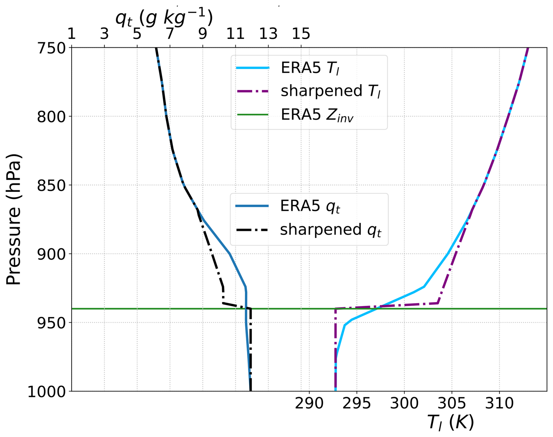
Figure A1 Vertical profiles of q_t and T_l from ERA5, and the sharpened versions of these profiles used to initialize the Sandu 2010 (4 July 2018) trajectory.