Particle flux–gradient relationships in the high Arctic: emission and deposition patterns across three surface types

The Arctic is experiencing a warming much faster than the global average and aerosol–cloud–sea–ice interactions are considered to be one of the key features of the Arctic climate system. It is therefore crucial to identify particle sources and sinks to study their impact on cloud formation and cloud properties in the Arctic. Near-surface particle and sensible heat fluxes were measured using the gradient method during the ARTofMELT Arctic Ocean Expedition 2023. A gradient system was deployed to calculate sensible heat and particle fluxes over three different surface conditions: wide lead, narrow lead, and closed ice. To evaluate the gradient measurements, sensible heat fluxes and friction velocities were compared with eddy covariance data. The strongest mean sensible heat fluxes, ranging from 16 to 51 W m⁻², were observed over wide lead surfaces, aligning with measurements from the icebreaker. In contrast, closed ice surfaces had weak, often negative, sensible heat fluxes. Wide leads acted as a particle source, with median net particle emission fluxes of 0.09 × 10⁶ m⁻² s⁻¹. Narrow lead surfaces exhibited both net emission and net deposition, though the particle fluxes were weaker. Closed ice surfaces acted as a particle sink, with normalized fluxes around 0.06 cm s⁻¹. The gradient method was found to be effective for measuring both sensible heat and particle fluxes, allowing flexible deployment over different surface types. This study addresses the critical need for improved quantification of turbulent vertical particle fluxes and related processes that influence the local particle number budget in the high Arctic.

1 Introduction

The Arctic is experiencing a warming four times faster than the global average due to increased emissions of greenhouse gases, particles and other climate drivers (Rantanen et al., 2022; Meredith et al., 2019). This phenomenon, known as Arctic amplification (Wendisch et al., 2023), is driven by various feedback and forcing mechanisms, e.g., the ice-albedo feedback (Hall, 2004) and the long-wave greenhouse effect of low-level mixed-phase clouds (Wendisch et al., 2019). Short-lived climate forcers like methane, tropospheric ozone and aerosols also contribute to this enhanced change (AMAP, 2021). Atmospheric aerosols exert an influence on the Earth's surface energy budget through two distinct effects. The direct effect involves scattering and absorption of incoming solar radiation (Charlson et al., 1991). The indirect effect occurs when particles act as cloud condensation nuclei or ice nuclei particles, leading to the formation of clouds and changes in cloud properties (Twomey, 1977; Albrecht, 1989). In the summertime high Arctic, particle number concentrations can be occasionally too low to facilitate cloud formation (Mauritsen et al., 2011; Stevens et al., 2018). Hence, it can be concluded that even small anthropogenic or natural sources of aerosols can exert a considerable influence on cloud cover, surface temperature, ice melt or freezing and thus on Arctic climate. It is therefore essential to gain a more detailed understanding of natural Arctic aerosol emissions, aerosol evolution and transport, as well as the effects on cloud microphysics (Schmale et al., 2021). There is still considerable uncertainty regarding the composition and formation pathways of high Arctic aerosol (Schmale et al., 2021; Lawler et al., 2021). Climate projections of future warming may be oversimplified and even miss processes, in part because of uncertainties about aerosols and their role in cloud formation (Chylek et al., 2016). Furthermore, there is a scarcity of turbulent flux measurements of particles and aerosol precursor gases in Arctic regions, which are crucial for constraining models of Arctic aerosol formation and emission (Willis et al., 2018; Schmale et al., 2021). It is therefore of great importance to improve the quantification of vertical turbulent particle fluxes and other processes contributing to the local particle number budget in the central Arctic region (Saylor et al., 2022).

The characterization of aerosol fluxes over sea ice, especially in the higher Arctic, remains incomplete, both in terms of observations and models (Schmale et al., 2021). Scott and Levin (1972) were the first to identify leads in the Arctic as a local source of atmospheric particles. The first quantification of aerosol fluxes over sea ice in the higher Arctic was conducted by Nilsson and Rannik (2001) and Nilsson et al. (2001), and later quantifications were conducted by Held et al. (2011a, b). Notable flux measurements in the higher Arctic on land have been made by Donateo et al. (2023), while Grönlund et al. (2002) and Contini et al. (2010) have made particle flux measurements in Antarctica. Nevertheless, very few measurements of aerosol fluxes on the sea ice have been made and additional flux measurements are needed to quantify particle sources and sinks. Difficulties arise, particularly, from the need for particle measurements with a high temporal resolution of, ideally, 10 Hz, which is essential for flux measurements to capture the fine-scale fluctuations of small variations, combined with the challenge of low particle concentrations. In addition to the first-order time response of the device, fluctuation dampening of the inlet must also be taken into account and is often the limiting factor (Conte et al., 2018). An alternative method for measuring fluxes in challenging environmental conditions, such as the sea ice, is the gradient method, which is based on the theory of flux–profile relationships (Held et al., 2011b; Farmer et al., 2021). The gradient method has been applied in different areas. On moving platforms like ships, the gradient method was applied, e.g., by Petelski (2003), Petelski et al. (2005) and Petelski and Piskozub (2006). Multi-year measurements using the gradient method have been made, for example, by Markuszewski et al. (2024). Assuming that turbulent fluxes are constant with height in the surface layer, the fluxes of momentum, heat and particles can be determined from vertical gradients of the mean quantities of wind speed, temperature and particle number concentration close to the surface (Foken and Mauder, 2024).

The present study is focused on near-surface particle and sensible heat fluxes, which were measured using a gradient system on ice floes in the Arctic spring. Variations in turbulent fluxes are examined in the context of surface characteristics, meteorological conditions and particle number concentrations. Our results can be used to identify turbulent particle exchange under the influence of different surface types and help to constrain Arctic aerosol sources and sinks in climate models.

2 Data and methods

This study is based on observations collected during the ARTofMELT (Atmospheric Rivers and the Onset of Arctic Sea Ice Melt) expedition in the Arctic Ocean in spring 2023 on the Swedish icebreaker Oden. The overarching goal of the expedition was to investigate the processes leading to the onset of sea ice melt and to explore its links to narrow filaments of poleward-moving warm and moist air, so-called atmospheric rivers (Tjernström and Zieger, 2025; Swedish Polar Research Secretariat, 2024). Oden departed from Svalbard on 8 May and returned to Svalbard on 15 June 2023. Particle flux and sensible heat flux data collected during two ice camps will be presented here. The first ice camp took place from 16 to 21 May on an ice floe at 79.6° N, 1.3° W and the second from 29 May to 11 June at 79.8° N, 2.8° E. Additional data analyzed in this study are derived from a wide range of measurements made on board Oden, including: 6-hourly radiosoundings, friction velocities and sensible heat fluxes by eddy covariance, and aerosol physical and chemical properties. Additional measurements were made on the ice floe, including friction velocity and sensible heat fluxes by eddy covariance and up- and downwelling radiative fluxes.

Profile measurements with the gradient setup, hereafter referred to as the gradient system, were made during the ARTofMELT ice camps on 16 d in total (Table 1). The runtime per day varied from 2.5 to 18 h, depending on access to the ice floe to change batteries; this was sometimes limited because of weather conditions or polar bears in the vicinity. The gradient data have been divided into three categories based on the upstream surface type. These categories are

1. wide lead: extensive open water surface (influence area dominated by open water, Fig. A1a);

2. narrow lead: open water within leads within pack ice (mixed influence area affected by open water and ice, Fig. A1b);

3. closed ice: smooth snow-covered ice surfaces without ridges or melt ponds (Fig. A1c).

From 17 to 18 May, the gradient system was set up approximately 5 to 10 m away from a wide lead. From 20 to 21 May, the gradient system was close (around 20 m) to a narrow lead. From 29 May to 6 June, the gradient system was surrounded by a smooth snow-covered closed ice surface, and from 7 to 9 June it was again located near a narrow lead (see Table 1).

2.1 Sampling methodology

To measure near-surface particle concentration profiles, we used a 1.5 m high linear actuator (Fig. 1a) with a sensor board (Fig. 1b). The sensor board contained (I) an ultrasonic distance sensor (HC-SR04, AZ Delivery, Deggendorf, Germany) to measure the distance from the surface, with a sampling rate of 0.5 s⁻¹, (II) a PT100 precision resistance thermometer (Electrotherm, Geraberg, Germany) for air temperature measurements and (III) a simple hot wire anemometer for measuring wind speed and temperature (Rev. P, Modern Device, Brooklyn, NY, USA), each with a sampling rate of 1 s⁻¹. In addition to the in situ sensors, a 20 cm long, downward-facing stainless steel inlet (IV) with an inner diameter of 3 mm was mounted on the sensor board. The inlet was connected to a condensation particle counter (CPC 3007, TSI, St. Paul, MN, USA) with 205 cm long conductive silicon tubing with an inner diameter of 4.2 mm. The battery-operated CPC measured the total particle number concentration with a lower cut-off diameter of 10 nm, a temporal resolution of 1 s⁻¹ and a sample volume flow rate of 0.7 L min⁻¹. Isopropanol was used as the working fluid for the CPC. The linear actuator and the sensors were powered by batteries. A laptop for system control and data recording, batteries and the CPC were placed downwind of the gradient system in an aluminum box for weather protection. The gradient system was oriented into the wind, upwind of the ship. A tripod was used to stabilize the system and was positioned downwind of the gradient system, as long as the wind did not change direction during the measurement. A white plastic tarp served as the base for the tripod to prevent sinking due to melting snow. Three additional PT100 resistance thermometers were mounted on the tripod at heights of 8, 90 and 120 cm above the surface. These air temperature measurements were used for quality control of the moving PT100 sensor. For wind direction measurements, a small ultrasonic anemometer with a response time of 10 Hz (LI-550F TriSonica Mini, LI-COR Lincoln, NE, USA) was mounted at the top of the tripod on a horizontally aligned arm, 38 cm from the tripod. Data from a 90° wind direction sector centered on the instrument tripod and box with batteries and logging system are excluded from the analysis because of flow distortion generated by these obstacles. The use of snow scooters and other potentially polluting activities were minimized during measurement periods. Measurement periods affected by pollution were determined by rapidly increasing particle concentrations and were excluded from the analysis.

The gradient system was programmed to approach six different height levels consecutively, starting from the bottom, with a distance of 5 cm between the inlet and the surface, followed by distances of 10, 17, 32, 67 and 129 cm. These heights varied by ± 1 cm, depending on the measurement and surface conditions. During descent from 129 to 5 cm, one additional measurement was taken at 32 cm above the surface, serving as an additional reference to track changes in background particle number concentration, but was not included in the gradient calculations. Height levels were changed every 50 s, resulting in a new profile cycle every 350 s.

In addition to the profile measurements with the gradient system, continuous eddy covariance sensible heat flux measurement (Prytherch et al., 2024) was carried out with sonic anemometers on a mast on the foredeck of Oden at a height of 20.3 m (referred to as the ship mast, Sonic: Metek u-sonic 3) and on a mast on the ice (Guy et al., 2024) at a height of 4 m (referred to as the ice mast, Sonic: Metek USA-100). Eddy covariance calculations followed standard procedures, including despiking, double coordinate rotation and linear detrending. Motion correction and a correction to compensate for flow distortion were also applied for the ship mast data (Prytherch et al., 2015). The additional eddy covariance measurements enable a comparison between the sensible heat fluxes and friction velocities (u^*) of the different setups. The sensible heat fluxes and friction velocities for the ship mast and ice mast sites were averaged over 20 min. For direct comparison, the data of the gradient system were also averaged over 20 min. The meteorological data for the periods in Table 1 were measured on the seventh deck of Oden at a height of approximately 25 m above sea level (Murto et al., 2024). General meteorological conditions during the AoM expedition were categorized in six periods, mainly defined using temperature and humidity profiles from 6-hourly radio soundings as well as 7 d back-trajectories, calculated with the Lagrangian Analysis Tool LAGRANTO on ERA5 data (see also Table 1; Murto et al., 2024; Murto and Tjernström, 2024). Radiation was measured at the ice mast site, from a radiometer stand at approximately 40 m from the ice mast (Guy et al., 2024).

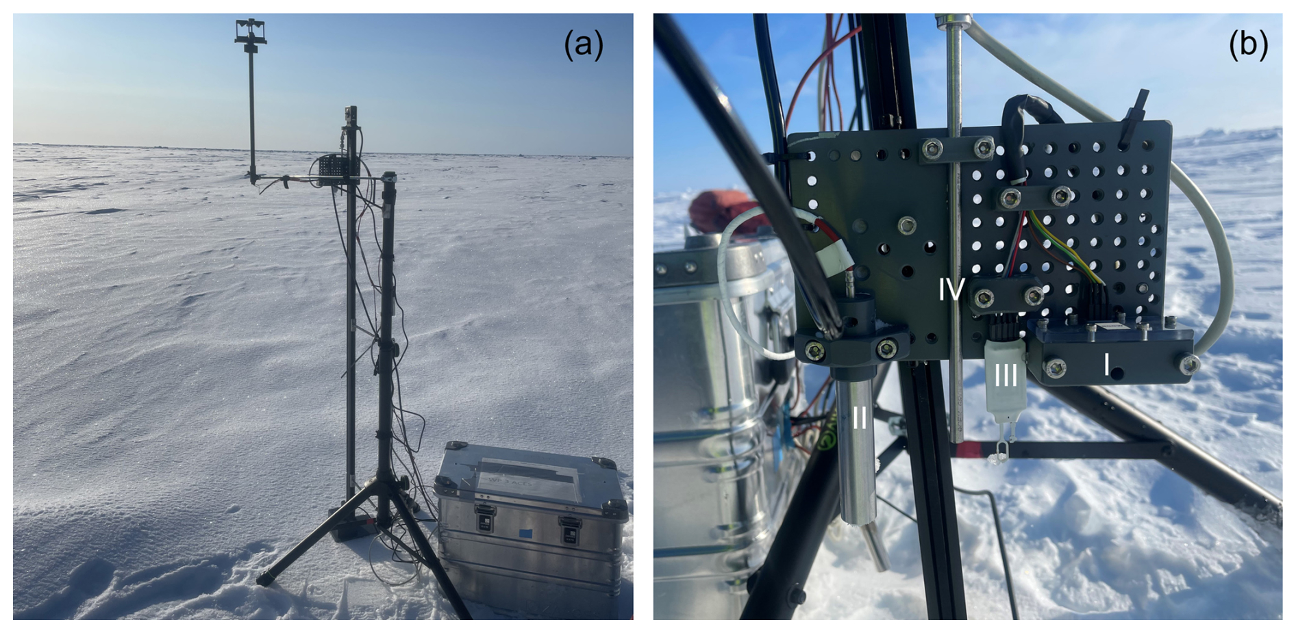
Figure 1 (a) Setup of the near-surface gradient system and (b) sensor board: (I) distance sensor, (II) PT100 precision resistance thermometer, (III) hot wire anemometer and (IV) the aerosol inlet. The sensor board was attached to the linear actuator.

2.2 Data analysis

Firstly, the height level of the gradient system was checked using the distance sensor data. The profile was used for further analysis if more than 80 % of the height data measured by the distance sensor were within ±  20 % of the set heights. In order to take into account the response time of all sensors, as well as the traveling time of the gradient system to the next height level, the first 20 s of each 50 s measurement interval at each height level were discarded. The CPC fully adjusted to a new particle number concentration within 9 s and the maximum traveling time to the next height level was 10 s. Therefore, only the last 30 s of the measured values per height level were used for further data analysis. Secondly, outliers were removed if values were outside 1.5 times the interquartile range of a moving 20 min window. The 20 min interval was chosen to avoid over-emphasizing short-term fluctuations, while still taking into account longer-term changes. The arithmetic mean over 30 s for each height level was calculated for further analysis. Thirdly, the wind speed data measured by the hot wire anemometer and the small ultrasonic anemometer, as well as the temperature data measured by the PT100 precision resistance thermometer and the hot wire thermocouple, were compared. For the wind, we assume a logarithmic profile with height. By linear regression of wind speed and logarithmic height, the measurements from the hot wire anemometer were extrapolated to 170 cm, the height of the sonic anemometer. For temperature, the sensors for comparison were already at the same heights as the profile measurements. Based on the calculated offsets between the sonic anemometer or PT100 precision resistance thermometer and the hot wire thermocouple, the data were adjusted so that only the hot wire anemometer data were used for the following analyses.

In the last step, the measured particle number concentrations were corrected for particle losses inside the tubing and inlet. In particular, small particles are lost by diffusion to tubing and inlet walls (Kulkarni et al., 2011). The diffusional losses were calculated following Gormley and Kennedy (1949). To determine the penetrating fraction as a function of particle size, the particle number size distribution between 15 and 792 nm, with a temporal resolution of 12 min, measured with a differential mobility particle sizer (DMPS) on the fourth deck of Oden was used. The inlet was a 4 m long heated whole air inlet, located approximately 25 m above sea level. Periods influenced by pollution from the ship's exhaust were excluded based on the derivative of the total particle number, following a similar principle to that described by Beck et al. (2022). The data were corrected for losses due to diffusion, sedimentation and inertial deposition, using the loss calculator of Von Der Weiden et al. (2009). It was assumed that the particle size distribution determined with the DMPS was representative of the size distribution entering the gradient system, given the absence of these measurements on the ice. For each size channel and the inlet characteristics described in Sect. 2.1, the loss rate was determined. The size-dependent loss rates per size channel were then multiplied by the normalized size distribution data and the total particle penetration efficiency was estimated by the sum of the adjusted normalized DMPS data. The hourly median penetrating particle fraction was found to be between 90 % and 98 %, with an overall median of 96 %. This variation is to be expected, due to the strong dependence on the size distribution (Kulkarni et al., 2011). To correct for diffusional particle losses, the measured particle number concentration of the gradient system was divided by the penetrating particle fraction value.

Evaluating the gradients from ascending stepped profiles produces a potential source of bias if the particle number concentration, wind speed and temperature change strongly during one full profile cycle of 350 s. Therefore, the particle and sensible heat flux were evaluated as mean trends for intervals of 20 min. For this purpose, 20 min intervals were created. For each 20 min interval, the median time point was determined and it was checked that at least five of the six heights within the 20 min were correctly measured by the gradient system. Linear interpolation based on time was used to determine the corresponding value at the median time point for the three measurements of particle number concentration, wind speed and temperature. The data analysis performed is shown step by step in Fig. A2.

2.3 Flux–profile relationships

Turbulent fluxes are considered to be constant with height in the surface layer (Holton and Hakim, 2013). Following the Monin–Obukhov similarity theory (Foken and Mauder, 2024), flux–gradient relationships for momentum flux, sensible heat flux (H) and particle flux (P) are

$$\begin{array}{}\text{(1)}& {\displaystyle }\stackrel{\mathrm{‾}}{U{}^{\prime }w{}^{\prime }}& {\displaystyle }=-K_m{\displaystyle \frac{\partial \stackrel{\mathrm{‾}}{U}}{\partial z}},\text{(2)}& {\displaystyle }H=\stackrel{\mathrm{‾}}{w{}^{\prime }T{}^{\prime }}& {\displaystyle }=-K_H{\displaystyle \frac{\partial \stackrel{\mathrm{‾}}{T}}{\partial z}},\text{(3)}& {\displaystyle }P=\stackrel{\mathrm{‾}}{w{}^{\prime }C{}^{\prime }}& {\displaystyle }=-K_P{\displaystyle \frac{\partial \stackrel{\mathrm{‾}}{C}}{\partial z}},\end{array}$$

where the momentum flux $\stackrel{\mathrm{‾}}{U{}^{\prime }w{}^{\prime }}$ is the covariance of turbulent fluctuations of the horizontal wind speed U (m s⁻¹) and vertical velocity w (m s⁻¹), and K_m is the turbulent diffusion coefficient for momentum. The sensible heat flux (H) $\stackrel{\mathrm{‾}}{w{}^{\prime }T{}^{\prime }}$ is the covariance of the turbulent fluctuations of vertical wind speed w and temperature (K) and K_H is the turbulent diffusion coefficient for sensible heat. To convert the kinematic sensible heat flux to units of W m⁻² we multiplied the value in units of K m s⁻¹ by the density of air (1.225 kg m⁻³) and the specific heat capacity (1005 J kg⁻¹ K⁻¹) of air. The particle flux (P) $\stackrel{\mathrm{‾}}{w{}^{\prime }C{}^{\prime }}$ is the covariance of the turbulent fluctuations of vertical wind speed w and particle number concentration C (cm⁻³) and K_P is the turbulent diffusion coefficient for particles. The measurement height is z (m). Based on the mixing length model (Foken and Mauder, 2024), K_m is often parameterized using

$$\begin{array}{}\text{(4)}& K_m=\mathit{\kappa }\cdot z\cdot u^{*},\end{array}$$

where κ is the von Kármán constant (=0.40), z is the measurement height and u^* is the friction velocity, which can be derived from the wind profile measurements according to

$$\begin{array}{}\text{(5)}& u^{*}=\sqrt{-\stackrel{\mathrm{‾}}{U{}^{\prime }w{}^{\prime }}}=\mathit{\kappa }\cdot z\cdot {\displaystyle \frac{\partial U}{\partial z}}=\mathit{\kappa }{\displaystyle \frac{\partial U}{\partial \ln z}}.\end{array}$$

In previous studies, values between 1.0 and 1.39 were found for the ratio $K_H/K_m$ (e.g., Foken and Mauder, 2024). Assuming K_m = K_H = K_P (e.g., Wieringa, 1980; Held et al., 2011b), the sensible heat flux (H) and the particle flux (P) are obtained from the profile measurements by

$$\begin{array}{}\text{(6)}& {\displaystyle }H=\stackrel{\mathrm{‾}}{w{}^{\prime }T{}^{\prime }}& {\displaystyle }=-\mathit{\kappa }\cdot u^{*}\cdot {\displaystyle \frac{\partial T}{\partial \ln z}},\text{(7)}& {\displaystyle }P=\stackrel{\mathrm{‾}}{w{}^{\prime }C{}^{\prime }}& {\displaystyle }=-\mathit{\kappa }\cdot u^{*}\cdot {\displaystyle \frac{\partial C}{\partial \ln z}}.\end{array}$$

The friction velocity u^* was determined from the measured gradient of the wind speed (Eq. 5). The gradient was calculated from a linear regression of the five wind speeds against the five logarithmic heights of each profile. The temperature T and particle concentration C gradients were also determined by linear regression to calculate the sensible heat flux (H) and the particle flux (P). Figure A3 shows (a) one measured particle concentration profile and (b) one wind speed profile, as well as the linear regression fits. The sensible heat flux (H) is defined as positive or upward if T decreases with increasing height. A positive particle flux (P) is defined as upward when C decreases with increasing height.

The calculation of fluxes from the mean gradients as described here assumes neutral stability; for stable or unstable stratification, stability corrections are required (Foken and Mauder, 2024). The need for a stability correction can be evaluated via the stability parameter $z/L$, where L is the Obukhov length:

$$\begin{array}{}\text{(8)}& L=-{\displaystyle \frac{u^{*\mathrm{3}}}{\mathit{\kappa }\frac{g}{T}\stackrel{\mathrm{‾}}{w{}^{\prime }T{}^{\prime }}}}\end{array}$$

where g is the gravitational acceleration (=9.81 m s⁻²), and T is the temperature. Positive values for the stability parameter $z/L$ indicate stable stratification, negative values refer to unstable conditions and neutral stratification is given by a value close to 0. To test whether the assumption of neutral stratification is justified, $z/L$ values were calculated for the gradient system and indicated for the interquartile range values of $-\mathrm{0.0024}<z/L<\mathrm{0.0357}$. Therefore, a majority of the measurements were taken under near-neutral conditions and we can ignore stability correction functions for Eqs. (5)–(7) and accept a <9 % error.

In the case of stable stratification, strong temperature gradients can occur very close to the surface. In order to determine periods with possible vertical decoupling, a decoupling metric based on the Brunt–Väisälä frequency has been calculated (Foken, 2023; Peltola et al., 2021). While the decoupling metric indicates coupled or weakly coupled periods when measuring at the wide lead, decoupling is frequently possible when measuring over closed ice surfaces. In order to exclude periods with weak turbulence and thus a high probability of vertical decoupling, the fluxes calculated from the gradient system were classified according to u^*. For further discussion of the turbulent particle and sensible heat fluxes according to the flux–profile relationships, all mean and median values, as well as the number of intervals, are based on periods when $u^{*}\ge \mathrm{0.15}$ m s⁻¹.

Applying the profile equation for u^* (Eq. 5) from a height z₀, at which the horizontal wind speed of the extrapolated logarithmic wind profile becomes zero, to the height z gives

$$\begin{array}{}\text{(9)}& U\left(z\right)-U\left(z_{\mathrm{0}}\right)=U\left(z\right)={\displaystyle \frac{u^{*}}{\mathit{\kappa }}}\cdot \ln {\displaystyle \frac{z}{z_{\mathrm{0}}}}.\end{array}$$

The roughness length z₀ is determined by rearranging Eq. (9):

$$\begin{array}{}\text{(10)}& z_{\mathrm{0}}=\exp \left(\ln \left(z\right)-{\displaystyle \frac{\mathit{\kappa }U}{u^{*}}}\right).\end{array}$$

To allow interpretation of particle fluxes independently of varying particle number concentrations and for comparison with other studies, a normalized flux, V_D [cm s⁻¹], is calculated:

$$\begin{array}{}\text{(11)}& V_D=-P/C.\end{array}$$

For reasons of comparability with other studies and the often-used deposition velocity, a positive normalized flux indicates a net deposition flux. To emphasize that we do not only refer to deposition processes, we use the term normalized flux for V_D.

Notably, the relative measurement uncertainties are large for small fluxes; this is common in the Arctic due to low particle number concentrations. The mean standard deviation (SD) of the 1 s⁻¹ measurements at a given height was highest for the particle number concentration, ranging from 3 % to 21 %, followed by temperature (ranging from 1 % to 10 %) and wind speed (ranging from 2 % to 7 %). The standard deviation was calculated for each individual height level; in the following, the mean standard deviation across all height levels for 1 d is used. Monte Carlo simulations were utilized to estimate the uncertainty of the flux estimate due to the measurement uncertainty. For each profile, 10 000 values, within the mean standard deviation of that day around the mean value, were randomly generated for each height level, based on the measured value for particle number concentration, temperature and wind speed. The fluxes were then determined 10 000 times with the ensemble of randomly generated values for temperature and particle number concentration, as well as u^* calculated from the wind speed gradient. The 90th percentile of the Monte Carlo simulated fluxes was calculated for each profile (Watanabe and Pfeiffer, 2022). The median of the 90th percentiles for 1 d was then used as the overall uncertainty (maximum error value) for that day. The median errors are 0.9 (SD ± 2.2) W m⁻² for the sensible heat flux and 0.27 (SD ±  0.38) × 10⁶ m⁻² s⁻¹ for the particle flux.

3 Results and discussion

The particle concentrations varied on the different measurement days with different surface types. During the phase when the gradient system was influenced by wide leads, the mean particle number concentration was around 197 cm⁻³ (see Table 1). For the closed ice measurement phase, the concentration was between 10 and 369 cm⁻³. When the measurements were influenced by narrow leads, the mean particle number concentration was between 77 and 122 cm⁻³. In the meteorological period 4, characterized by cool and dry northerly winds, the particle number concentration was notably low at 10 and 37 cm⁻³. The particle number concentration also decreased in the transition from period 2 to period 3, from 18 to 20 May. This was characterized by a change in wind direction from north-westerlies/south-westerlies to southerly winds and mild and moist conditions, which resulted in a temporary warming period. Prior to the onset of melting on 10 June, northerly winds brought air masses with low particle number concentrations and mainly originated from over the pack ice (Murto and Tjernström, 2024). Wind from the west or east may indicate influence from terrestrial areas like Greenland or Svalbard, respectively.

For the wide lead, closed ice and narrow lead surface types, different values of the surface roughness length (z₀) are expected. From Eq. (10), the highest value of z₀ was found for the wide lead surface type, with a median of 4.9 × 10⁻³ m. Comparable values of lead areas between sea ice/polynyas show lower z₀ values of, e.g., 0.1–2.2 × 10⁻³ m (Held et al., 2011a) or 0.6–0.9 × 10⁻³ m (Nilsson and Rannik, 2001). Differences may be due to different footprints, which are not entirely influenced by leads. The lowest z₀ was found for the closed ice surface type, with a median value of 0.3 × 10⁻³ m. These results are in agreement with the z₀ values determined in the high Arctic by Nilsson and Rannik (2001) and Persson et al. (2002), which indicate a flat ice surface unaffected by other factors. The mixed narrow lead surface type had z₀ values around 1 × 10⁻³ m, also agreeing with measurements by Held et al. (2011a), Andreas et al. (2010), and Nilsson and Rannik (2001).

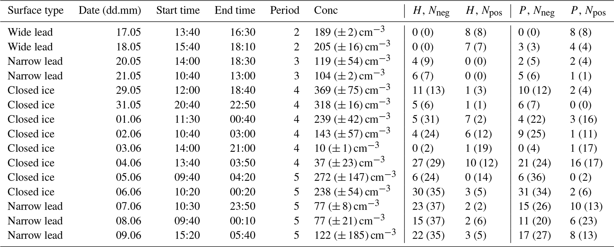
Table 1 Overview of the measurement phases from 17 May to 10 June 2023 on various surface types. The start and end times (given in UTC) describe the measurement period, although this may be interrupted for several hours by battery power failures and may continue into the next day. The meteorological periods (2 = cold, north-westerlies/south-westerlies; 3 = mild and humid, first temporary warming, southerly winds; 4 = cooler and drier, mostly northerly winds, 5 = almost melting, warm and dry air at altitude, west winds) describe the meteorological conditions, determined for the entire expedition based on radiosonde data, trajectories, wind direction and wind speed (Murto et al., 2024; Murto and Tjernström, 2024). The column Conc describes the median particle number concentration (independent of the u^* ≥ 0.15 m s⁻¹ filter) with standard deviation and the final four columns show how many 20 min intervals of that day were dominated by net positive (upward) and net negative (downward) flux measurements for sensible heat flux (H) and particle flux (P). The values in parentheses refer to the total number; the values outside the parentheses refer to intervals with $u^{*}\ge \mathrm{0.15}$ m s⁻¹.

3.1 Friction velocity and sensible heat flux

The gradient method is evaluated against the eddy covariance method by comparing the friction velocity (u^*) and the sensible heat flux (H) determined by the gradient system with the same parameters determined on the ship (ship mast) and the ice (ice mast) by eddy covariance. It must be kept in mind that different footprints result from the different locations and heights of the measurements at 20 m (ship mast), 4 m (ice mast) and 1 m (gradient system) and their surrounding surface types; thus, a perfect agreement cannot be expected.

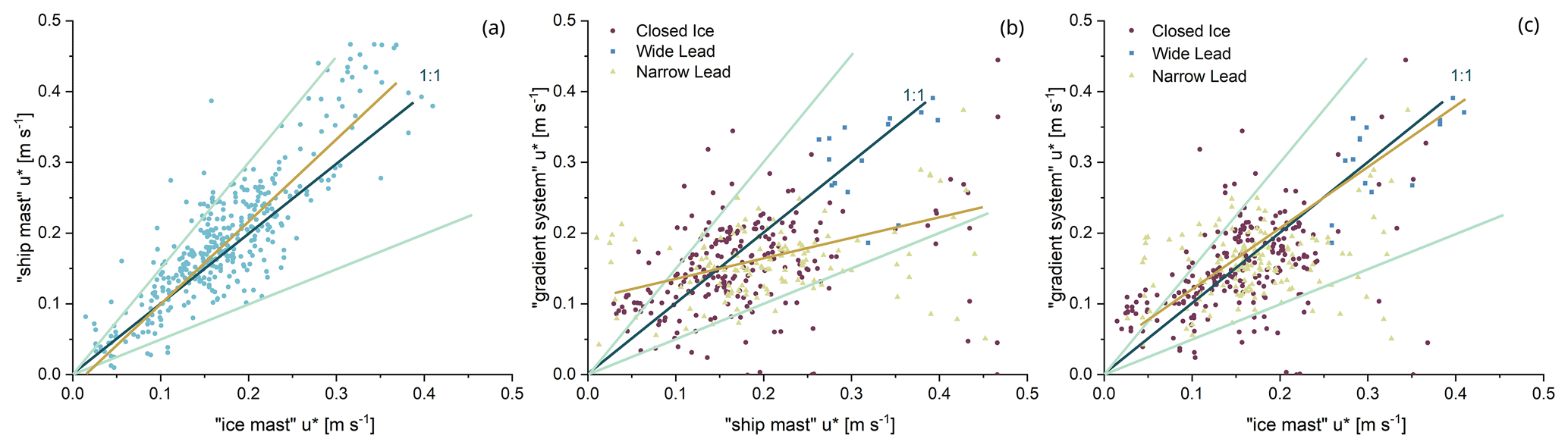
Figure 2 (a) Scatter plot between friction velocities [u^*, m s⁻¹] measured by the ship mast (y-axis) and the ice mast (x-axis). (b) Scatter plot between friction velocities measured by the gradient system (y-axis) and the ship mast (x-axis). (c) Scatter plot between friction velocities measured by the gradient system (y-axis) and the ice mast (x-axis). The dark blue lines symbolize the 1:1 line, the turquoise lines the 50 % deviations. The beige line shows the linear regression fit. The three different symbol colors in (b) and (c) divide the measurements according to the surface type, which influenced the gradient system.

The absolute differences of the u^* values are almost always within 0.1 m s⁻¹ for the whole dataset and, notably, the variation of the difference of u^* measured on the ship mast and on the ice mast by eddy covariance is similar to the variation of the differences between the gradient system and the eddy covariance systems. The median deviation of u^* between the gradient system and the ship mast is 0.02 m s⁻¹ and between the gradient system and the ice mast it is 0.04 m s⁻¹. The median of the differences between two eddy covariance datasets from ship mast and ice mast is only slightly smaller, at 0.01 m s⁻¹. The results demonstrate that the eddy covariance measurements on the ship mast and ice mast show the highest degree of agreement (Fig. 2a). Nevertheless, as can be seen in Fig. 2c, many of the u^* values determined at the ice mast and gradient system sites are in good accordance and close to the 1:1 line. In particular, when both systems are influenced by the same surface type (closed ice), there is good agreement of u^*. The agreement of the u^* values determined at the ship mast and gradient system sites (Fig. 2b) is slightly lower, but still consistent with expectations. The deviation of u^* between the gradient system and ship mast measurements was less than 50 % in 63 % of the cases. The deviation of u^* between the gradient system and ice mast measurements was less than 50 % in 77 % of the cases, and that between the ship mast and ice mast was less than 50 % in 89 % of the cases. The comparison includes all data, also when $u^{*}<\mathrm{0.15}$ m s⁻¹.

The comparison of the sensible heat fluxes between the three systems shows the dependence of the sensible heat flux on the type of surface surrounding the system (Fig. 3b, c). As for the friction velocity, the ship mast and ice mast sites (Fig. 3a), both evaluated with the eddy covariance method, show the highest degree of agreement. The comparison between the ice mast and gradient system shows that, for the narrow lead surface type, the fluxes differ in sign and thus in direction. Also, when the gradient system is influenced by wide leads, clear differences can be seen; this is to be expected, due to the different surface types influencing the two systems. However, when influenced by the same surface type (closed ice), the values are of the same magnitude (Fig. 3c). When comparing the gradient system with the ship mast (Fig. 3b), the opposite sign is also evident for the narrow lead. For the wide lead, high positive sensible heat fluxes are observed with both systems. This is consistent with the ship mast being surrounded by wide leads at the same time as the gradient system.

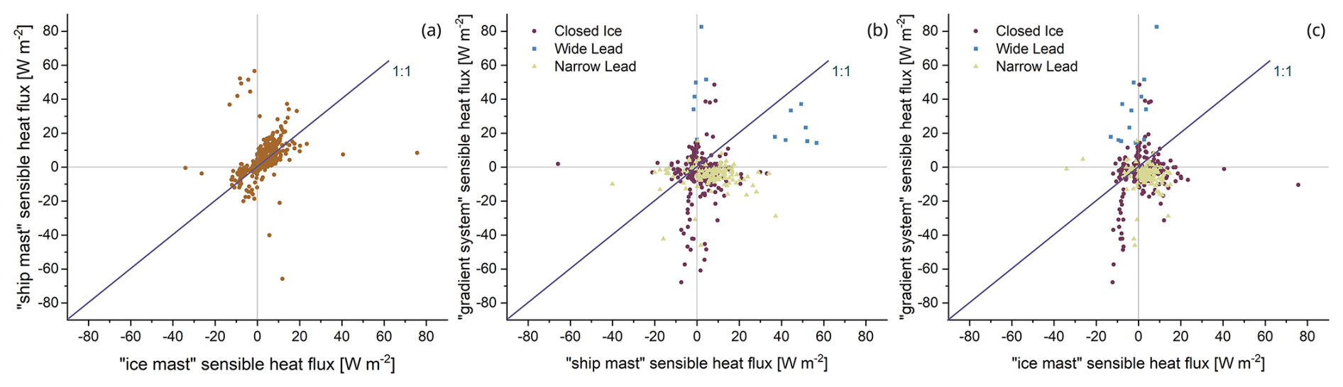
Figure 3 (a) Scatterplot between sensible heat fluxes [H, W m⁻²] measured by the ship mast (y axis) and the ice mast (x axis). (b) Scatterplot between sensible heat fluxes measured by the gradient system (y axis) and ship mast (x axis). (c) Scatterplot between sensible heat fluxes measured by the gradient system (y axis) and ice mast (x axis). The dark blue lines symbolize the 1:1 line. The three different colors in (b) and (c) divide the measurements according to the surface type, which influenced the gradient system.

Figure 4a and b show sensible heat fluxes measured with the gradient system with a time resolution of 20 min, as well as the 20 min fluxes measured with two eddy covariance systems, at the ice mast and ship mast. All measured values here are for conditions of $u^{*}\ge \mathrm{0.15}$ m s⁻¹. The most pronounced positive sensible heat fluxes were observed on 17 and 18 May by the gradient system, with 20 min mean values of 61 (SD ± 34) W m⁻² on 17 May (Fig. 4a) and 22 (SD ± 9) W m⁻² on 18 May, influenced by the wide lead surface type (Fig. 4b). Sensible heat fluxes from the ship mast, which was also surrounded by wide leads, were also strongly positive on 18 May, with 20 min mean values of 49 (SD ± 8) W m⁻². A decreasing temperature from the surface (open water −1 °C) to the top of the gradient system (−3 to −2 °C) can explain the positive sensible heat fluxes measured on these days. Similar results, although smaller in magnitude (sensible heat flux of 9 W m⁻²), have also been observed by Held et al. (2011b).

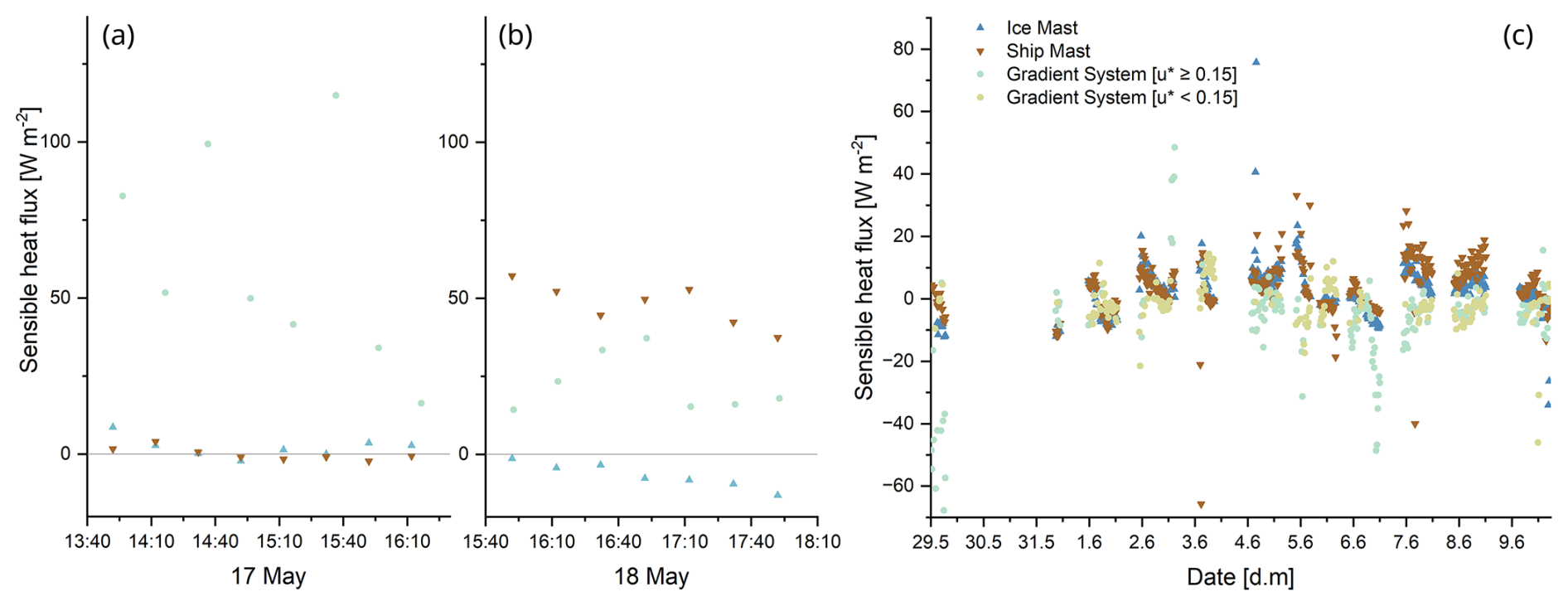
Figure 4 (a, b) Sensible heat flux [H, W m⁻²] on (a) 17 May and (b) 18 May 2023 from the gradient system setup influenced by wide leads with a time resolution of 20 min, as well as sensible heat flux from the ship mast and ice mast with a time resolution of 20 min. (c) Sensible heat flux from the second ice camp from 29 to 10 June 2023 from the three different measurement setups (gradient system, ice mast and ship mast). In (a) and (b), all $u^{*}\ge \mathrm{0.15}$ m s⁻¹; in (c), gradient system data are shown in different colors depending on u^*.

For a longer comparison of sensible heat fluxes measured with the eddy covariance and the gradient methods, Fig. 4c shows the sensible heat flux for the different measurement setups for the second ice camp. From 29 May to 5 June, the gradient system and the ice mast are surrounded by the same surface type (closed ice). At the beginning of June, sensible heat fluxes measured by the gradient system over the closed ice surface were very low. For this period, the low u^* (beige circles) indicates possible vertical decoupling. On 2 June, the mean net flux estimated from the gradient system and the ice mast was $H=-\mathrm{5}$ (SD±5) W m⁻², whereas H=4 (SD±4) W m⁻² was estimated from the ship mast. The colder ice surface, in contrast to the open water, leads to a change in the temperature gradient, resulting in lower fluxes. Most comparable studies found low positive values (Held et al., 2011b; Persson et al., 2002) and Sedlar et al. (2011) report mean values between −2 and 6 W m⁻². The difference between the gradient system and the ice mast/ship mast site on 5 June could be attributed to low turbulence, which is indicated by a small u^* of 0.04–0.21 m s⁻¹. In the final measurement phase, from 7 until 9 June, in which the footprint of the gradient system was defined by a mixed surface condition (narrow lead), the fluxes of the gradient system deviate strongly from those of the other measurement setups (Table 1). The calculated fluxes for the gradient system are negative, with an average flux of −7 (SD±5) W m⁻² for 7 June and −3 (SD±3) W m⁻² for 8 June. In contrast, the fluxes at the ice mast and ship mast locations are positive, at around H=5 (SD±5) W m⁻² and H=10 (SD±4) W m⁻². The discrepancy may be attributed to differences in surface conditions between the measurement setups, as well as to variations in the areas of influence resulting from the different measurement heights. It may be hypothesized that the ship mast footprint was characterized by a larger fraction of open water.

Spatially highly variable factors, such as cloud cover and the surface type, can have a direct and strong influence on the local sensible heat exchange (Sedlar et al., 2011; Held et al., 2011b; Lüers and Bareiss, 2010; Li et al., 2020). Sedlar et al. (2011) demonstrated that the surface energy budget is strongly influenced by the properties of the clouds and the degree of cloud cover. This is also a potential explanation for the notable differences observed in the results from the three measurement setups, which can be attributed to different upstream conditions for the different measurement sites. Measurements of the total up- and downwelling radiation, as well as the air temperature and the surface brightness temperature at the ice mast site (Guy et al., 2024), indicate a highly complex relationship between the surface heat flux and the radiation budget. The downwelling radiative flux of 950 W m⁻² and an upwelling radiative flux of 900 W m⁻² during midday (e.g., 21 May 2023) result in an increase in the surface brightness temperature. This coincides with a positive sensible heat flux around 12:00 UTC, which either decreases slightly or returns to zero overnight. This effect is either reduced or absent when cloud cover is increased. The strong influence of local-scale processes on the sensible heat flux in the Arctic is also emphasized by Liu et al. (2024) and Lüers and Bareiss (2010, 2011), among others.

3.2 Particle fluxes

In the following analysis of particle fluxes (P), again, a distinction is made between the wide lead, closed ice and narrow lead surfaces. Particle fluxes are influenced not only by the surface type but also by particle number concentrations present in the air (Nilsson and Rannik, 2001) and by the micrometeorological conditions, including the development of turbulence and atmospheric stability. Particle number concentration variations observed at a single location are attributable, among other factors, to the influence of varying meteorological conditions. To remove the influence of varying particle number concentrations, the normalized flux (in cm s⁻¹, e.g., Farmer et al., 2021) calculated according to Eq. (11) will also be presented. It should be emphasized that the observed particle fluxes are a combination of emission and deposition fluxes, i.e., net positive fluxes are dominated by particle emission and net negative fluxes are dominated by particle deposition.

As outlined in Sect. 2.3, the uncertainties of the calculated fluxes can be considerable. For a general understanding, it is thus instructive to first consider typical properties of the particle flux values as a function of surface type, rather than specific flux values. Table 1 gives an overview of how many 20 min intervals of each day were associated with net positive (upward) and net negative (downward) flux measurements.

3.2.1 Wide and narrow leads

Under the influence of wide leads on 17 May (Fig. 5a), all 20 min intervals are characterized by a positive net particle flux, indicating the net emission of particles (Table 1). On 18 May (Fig. 5b), this is the case for approximately half of the measurement time (Table 1). However, taking into account the estimated maximum uncertainty (gray shading in Fig. 5), fluxes may be positive or negative but with a tendency toward net particle emission. The median value of positive net fluxes is 0.12 × 10⁶ m⁻² s⁻¹ on 17 May and 0.02 × 10⁶ m⁻² s⁻¹ on 18 May. The normalized flux for the wide lead surface type on 17 May ranges from −0.09 to −0.04 cm s⁻¹ with a median value in terms of net emission of −0.06 cm s⁻¹.

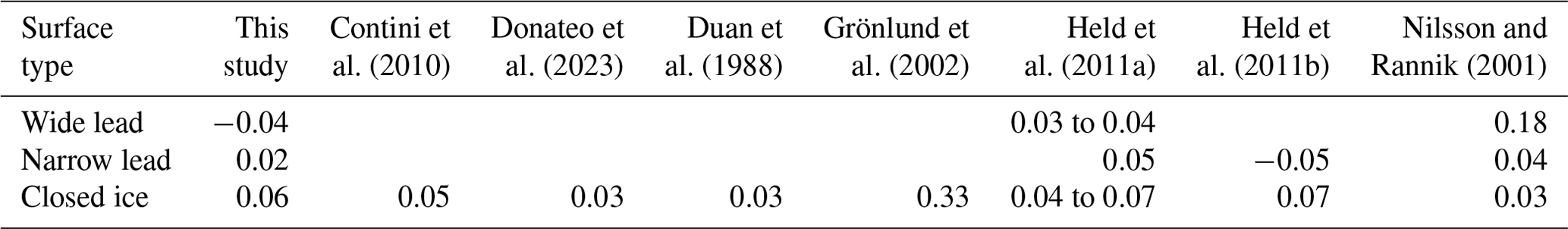
Table 2 Overview of the normalized fluxes of this study and comparable studies, depending on the surface type (in cm s⁻¹). Duan et al. (1988) report the mean value. All other studies report median values. The normalized fluxes of Held et al. (2011a) refer to deposition-dominated flux periods.

Concerning the narrow lead surface type, the first phase, from 20 to 21 May, is characterized by both positive and negative fluxes but mostly net particle deposition, with a median net deposition flux, of $-\mathrm{0.16}\times {\mathrm{10}}^{\mathrm{6}}$ m⁻² s⁻¹ on 20 May (Fig. 5c) to $-\mathrm{0.03}\times {\mathrm{10}}^{\mathrm{6}}$ m⁻² s⁻¹ on 21 May (Fig. 5d). It is evident that the uncertainty is much smaller than for the wide lead site and there are time periods that can be attributed to a specific flux direction outside of the maximum uncertainty. From 7 to 9 June (see Fig. A4a, b), all days are dominated by net particle deposition, with a median net particle deposition flux of $-\mathrm{0.03}\times {\mathrm{10}}^{\mathrm{6}}$ m⁻² s⁻¹. In total, 50 net deposition and 27 net emission intervals were observed under narrow lead conditions (Table 1). However, with both negative and positive particle flux values, the average flux can be close to zero and it is not possible to determine a preferred flux direction on this 3 d period. Rather, both net particle emission and deposition intervals may be observed under narrow lead conditions. The median normalized fluxes for particle deposition on 20 and 21 May are 0.80 and 0.03 cm s⁻¹, respectively. With regard to particle emission, the median normalized flux is observed to be in the range −0.05 to −0.03 cm s⁻¹ on 7 and 8 June, and −0.06 cm s⁻¹ on 9 June. The normalized flux at narrow leads determined by Held et al. (2011b) is in a similar range, from −0.008 to −0.1 cm s⁻¹, but is more dominated by emission processes. The normalized flux determined by Nilsson and Rannik (2001) ranges from 0.029 to 0.065 cm s⁻¹ (Table 2).

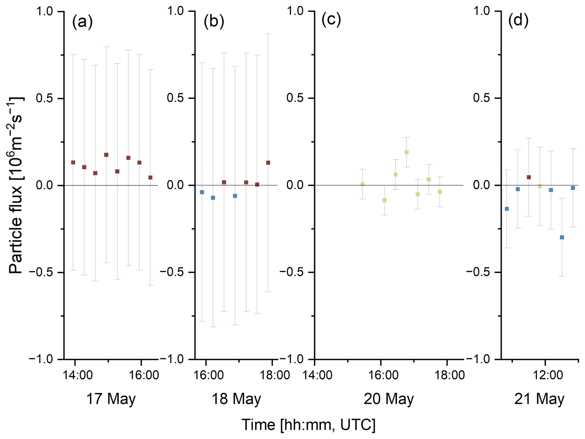
Figure 5 (a, b) Particle flux [P, 10⁶ m⁻² s⁻¹] at wide lead surface type on (a) 17 May and (b) 18 May 2023; (c, d) particle flux at narrow lead surface type on (c) 20 May and (d) 21 May 2023. The brown color indicates net particle emission intervals and the blue color indicates net particle deposition intervals. The beige color indicates intervals where $u^{*}<\mathrm{0.15}$ m s⁻¹. The gray-shaded bars illustrate the maximum error value for the day of measurement, as estimated by Monte Carlo simulations.

Compared with measurements over soil and water, there are few direct measurements of particle dry deposition over snow and ice surfaces (Willis et al., 2018; Emerson et al., 2020). In the literature, little distinction is made between the size of the leads and the fraction of open water. For open leads in the Arctic, Held et al. (2011a) and Nilsson et al. (2001) published comparable measurements. Our results are in agreement with previous studies that particles are emitted from leads (Lapere et al., 2024; Nilsson et al., 2001; Held et al., 2011a). Sometimes, however, net particle deposition at leads was also observed. Held et al. (2011a) found both net particle deposition and emission from leads, with fluxes of $-\mathrm{0.03}\times {\mathrm{10}}^{\mathrm{6}}$ to 0.02×10⁶ m⁻² s⁻¹. Nilsson and Rannik (2001) also recorded positive and negative fluxes across leads. Positive fluxes in the vicinity of leads had a median value of 0.032×10⁶ m⁻² s⁻¹ and negative fluxes had a median of −0.024 × 10⁶ m⁻² s⁻¹ (Nilsson and Rannik, 2001). When both positive and negative fluxes are included, the fluxes are not notably different from zero (Nilsson and Rannik, 2001); this was also observed in this measurement campaign. Held et al. (2011b) calculated fluxes of 0.006 × 10⁶ to 0.057×10⁶ m⁻² s⁻¹ using the gradient method and fluxes of $-\mathrm{0.02}\times {\mathrm{10}}^{\mathrm{6}}$ to 0.05×10⁶ m⁻² s⁻¹ using the eddy covariance method in the area affected by leads. Held et al. (2011a) detected almost equal numbers of deposition and emission events at leads.

Nevertheless, it is clear that the strongest net emission fluxes occur most frequently in the vicinity of sea water (Willis et al., 2018). It has been suggested in the literature that particle emissions detected over sea water consist of sea salt aerosols caused by wind-driven white caps and bubble bursts at the sea surface (Nilsson et al., 2001). Other studies suggest that the emission of particles from narrow leads/wide leads is not exclusively driven by wind (Held et al., 2011a); this is consistent with our observations. We could not find a clear correlation between increasing wind speed and a higher net particle emission flux (Fig. A6). This is also consistent with the observations of Scott and Levin (1972), who found open lead aerosol production without visible bubble activity. They speculated that very small bubbles could still be bursting at the interface between the atmosphere and the water and that droplets could be released from the bursting of micro-bubbles during melting or freezing processes. Norris et al. (2011) observed bubbles in the surface water of open leads, even during periods of low wind speed and when the lead was covered with ice.

3.2.2 Closed ice

For eight days, the gradient system was under the influence of closed ice. Net particle deposition dominated over emission for the majority of these eight days. Median net deposition fluxes are around $-\mathrm{0.02}\times {\mathrm{10}}^{\mathrm{6}}$ m⁻² s⁻¹, with a typical median normalized flux of 0.06 cm s⁻¹. On 29 (not shown) and 31 May (see Fig. 6a), as well as on 5 and 6 June (Fig. A5b), the particle fluxes are negative during nearly the entire measuring interval. However, it is possible that net emission fluxes may occur if the maximum estimated uncertainty (gray shading) is taken into account. Net particle emission dominated during 1 d (3 June), of which very small fluxes close to zero were observed on 3 June (see Fig. A5a) and 4 June. The lowest particle number concentrations during the entire expedition were observed during this 2 d period. The median normalized flux was between −0.09 and 0.23 cm s⁻¹ on 3 June and between −0.07 and 0.09 cm s⁻¹ on 4 June. In total, 87 net deposition and 25 net emission intervals were observed under closed ice conditions (Table 1). Given that the majority of net particle deposition occurs over the closed ice surface type, it can be concluded that the ice acts mainly as a sink in terms of particle number. Exceptions may be attributed to very low particle number concentrations on 3 and 4 June.

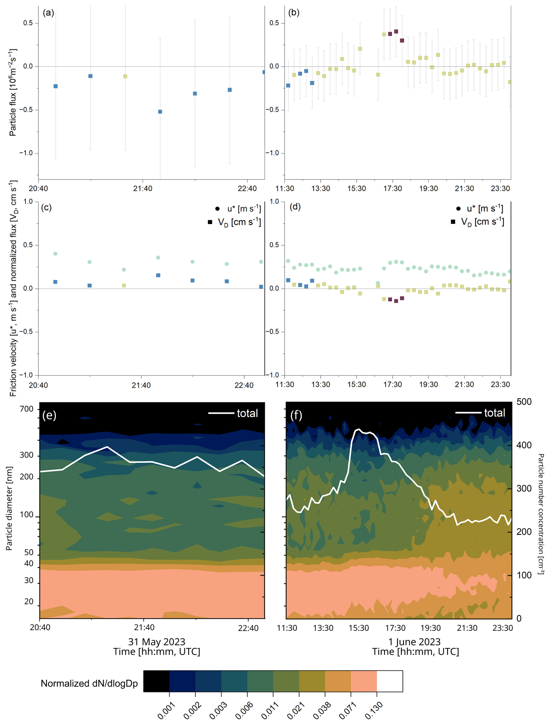
Figure 6 (a–d) Overview of surface type closed ice on 31 May and 1 June: (a, b) particle flux [$P,\times {\mathrm{10}}^{\mathrm{6}}$ m⁻² s⁻¹], (c, d) normalized flux [V_D, cm s⁻¹] and friction velocity [u^*, m s⁻¹]. The brown color indicates net particle emission and the blue color indicates net particle deposition. The beige color indicates intervals where $u^{*}<\mathrm{0.15}$ m s⁻¹. The gray-shaded bars illustrate the maximum error value for the day of measurement, as estimated by Monte Carlo simulations. The beige color shows the friction velocity. (e, f) Normalized $\mathrm{d}N/\mathrm{d}\log D_{\mathrm{p}}$ particle size distribution from 15 to 790 nm (left y-axis) with total particle number concentration, measured with a DMPS on the fourth deck of Oden (white line; right y-axis).

Net particle emission from a closed ice surface, like that on 1 June (Fig. 6b), has also been observed in other studies, e.g., in Nilsson et al. (2001). As particle fluxes and normalized fluxes are strongly dependent on particle size (Nilsson and Rannik, 2001), a changing size distribution (Fig. 6e, f) could explain a change from net particle deposition to net particle emission intervals. Due to Brownian diffusion, the normalized flux of particles with a diameter of less than 100 nm is greater than that for particles above 100 nm (Farmer et al., 2021; Nilsson and Rannik, 2001; Grönlund et al., 2002). The particle size distribution (measured on the ship) on 31 May shows a clear maximum of particles between 10 and 30 nm (Fig. 6e). However, the size distribution is different on 1 June (Fig. 6f); and also on 4 June (not shown). The number of particles in the 10–30 nm diameter range decreases, and an increase of larger particles with a diameter of 100 nm or above can be observed. A possible explanation for the change in particle size distribution could be a change in wind direction from north-east to north-west (Murto et al., 2024). On 1 June, it can be observed that, from 17:00 UTC, the concentration of particles in the diameter range up to 120 nm increases, and from 19:00 UTC the concentration of particles in the diameter range from 10–30 nm decreases (Fig. 6f). The net deposition flux before 16:00 UTC changes to a net emission flux after 17:00 UTC (Fig. 6b). Small particles with a high normalized flux, resulting in a net deposition flux close to the surface, become less dominant after 17:00 UTC; this could make previously masked emission processes visible. This effect is not associated with a change in friction velocity (Fig. 6d). Possible, albeit weak, particle sources from the closed ice surface could be secondary aerosol formed from dimethyl sulfide (Park et al., 2019; Kerminen and Leck, 2001), organic compounds (Moschos et al., 2022) or fine-mode sea salt aerosol generated by blowing snow (Gong et al., 2023; Yang et al., 2008, 2019). Sea salt aerosols, aerosols from dimethyl sulfide and organic aerosols are in the size ranges 10–300 nm (Gong et al., 2023), 50–100 nm (Ghahreman et al., 2019) and >100 nm (Tremblay et al., 2019), respectively, and could thus contribute to the observed particle emission flux. Sea salt aerosols and sublimation from blowing snow, as well as secondary organic aerosols, are considered more likely, as dimethyl sulfide has only been detected in sea water (Ghahreman et al., 2019) or in/near melt ponds (Gourdal et al., 2018), neither of which were present at this site. Wind speeds of more than 7 m s⁻¹ are required to generate sea salt aerosol from snow-covered ice surfaces, (Gong et al., 2023); these speeds were temporarily exceeded in the morning and early afternoon.

Comparing with particle fluxes above closed ice cover in previous studies, a normalized flux between −0.013 and 0.13 cm s⁻¹ was estimated from the gradient method and by eddy covariance during the ASCOS 2008 campaign on an ice floe (Held et al., 2011b; Table 2). Results from eddy covariance measurements at the Nansen Ice Sheet, Antarctica (Contini et al., 2010), in the MIZ (Held et al., 2011a; Nilsson and Rannik, 2001), over a closed snow surface in Pennsylvania (Duan et al., 1988) and in Ny-Ålesund (Donateo et al., 2023) are also within this range. Grönlund et al. (2002) found even higher normalized fluxes over a snow surface in Antarctica, with a mean particle normalized flux of 0.33 cm s⁻¹ (Table 2). Apart from the wide range of normalized fluxes observed, it is clear that the closed ice surface acts mainly as a sink for particles. Thus, very few emission-dominated intervals were observed under the influence of closed ice and the particle fluxes in these areas are mostly negative, indicating net particle deposition.

4 Summary and conclusions

Near-surface particle and sensible heat fluxes using the gradient method were successfully determined in the Arctic Ocean as part of the ARTofMELT expedition. A novel battery-powered gradient flux system facilitated measurement at multiple locations by relocating the instrument to quantify turbulent fluxes influenced by three different surface types, i.e., wide lead, narrow lead and closed ice.

The fluxes calculated by the gradient method were validated by comparing sensible heat fluxes and friction velocities measured with two eddy covariance systems. Positive sensible heat fluxes were high at the wide lead site, with median fluxes between 16 and 51 W m⁻², aligning closely with the eddy covariance flux observed on the ship mast (49 W m⁻²). For measurements influenced by closed ice, sensible heat fluxes were very weak, with slightly negative values.

Under the influence of wide leads, net particle emission fluxes in the region of 0.09×10⁶ m⁻² s⁻¹ dominated. The observations in this study clearly suggest that open water typically acts as a net particle source. In the presence of narrow leads, both net emission and net deposition fluxes were observed. With a median net particle emission flux of 0.02×10⁶ m⁻² s⁻¹ and a median net particle deposition flux of $-\mathrm{0.03}\times {\mathrm{10}}^{\mathrm{6}}$ m⁻² s⁻¹, the particle fluxes are close to zero and less pronounced than under the influence of wide leads. The closed ice surface, conversely, clearly acted as a net particle sink. Median net particle deposition fluxes were around $-\mathrm{0.1}\times {\mathrm{10}}^{\mathrm{6}}$ m⁻² s⁻¹, with a normalized flux of 0.06 cm s⁻¹. In periods with particularly low concentrations, with daily mean particle number concentrations of 10 cm⁻³, normalized fluxes up to 0.09 cm s⁻¹ were determined, although such low concentrations are associated with high uncertainties. On several occasions, net particle emission intervals occurred under the influence of closed ice. These emission events coincided with a shift in the diameter range of small particles from 10–30 to 100–200 nm. Possible emission sources from the ice include, for example, fine-mode sea salt aerosols generated by blowing snow.

Overall, this study provides additional experimental data to corroborate previous findings that different surface types have characteristic effects on the turbulent particle exchange between the atmosphere and the central Arctic Ocean. Furthermore, the gradient method was validated by comparison with simultaneous measurements from three different systems and two different techniques. Quantifying typical particle deposition fluxes to closed ice surfaces and typical particle emission fluxes from open leads can reduce the uncertainty in Arctic aerosol models. In order to obtain a representative dataset for the models, further measurements are required during different seasons, years and locations. The gradient system is an appropriate method for this purpose.

Appendix A

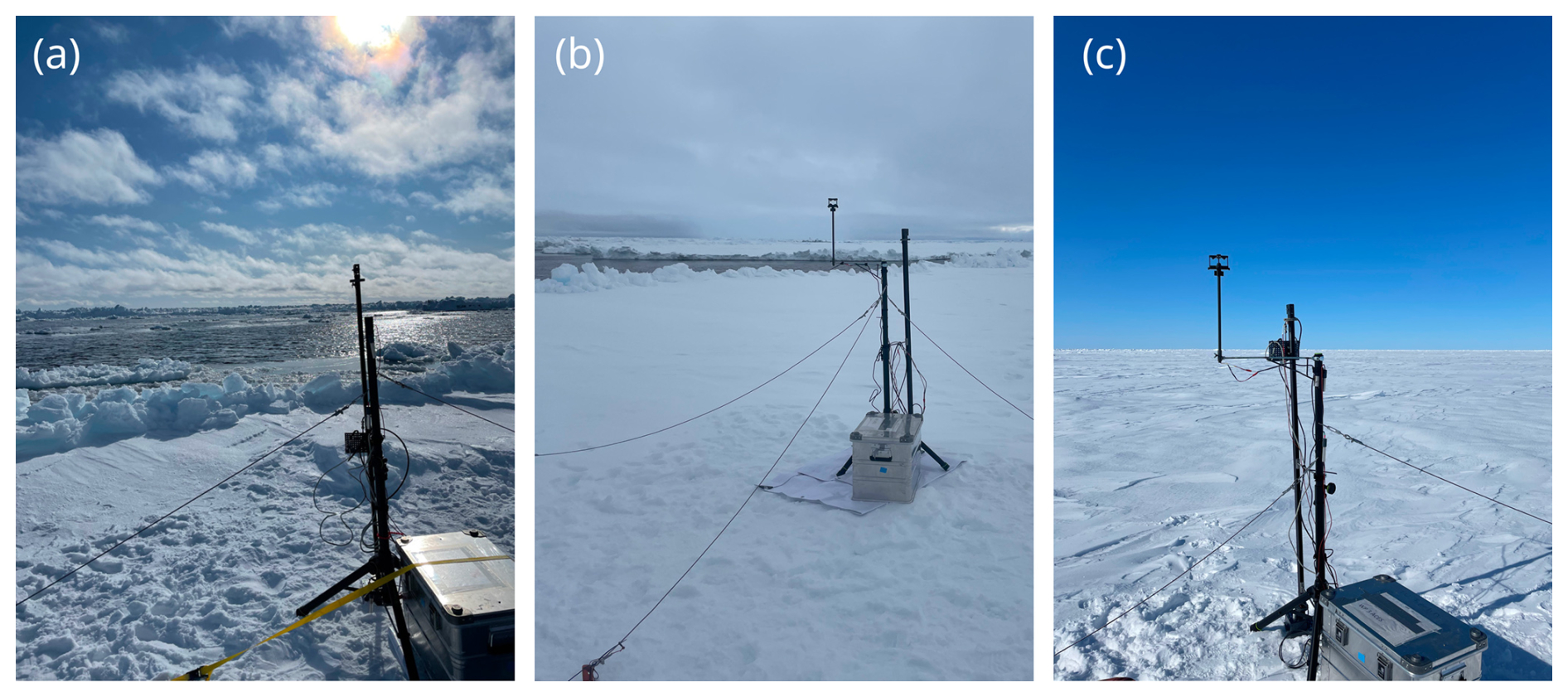
Figure A1 Three exemplary pictures of the studied surface types: (a) wide lead, (b) narrow lead, (c) closed ice.

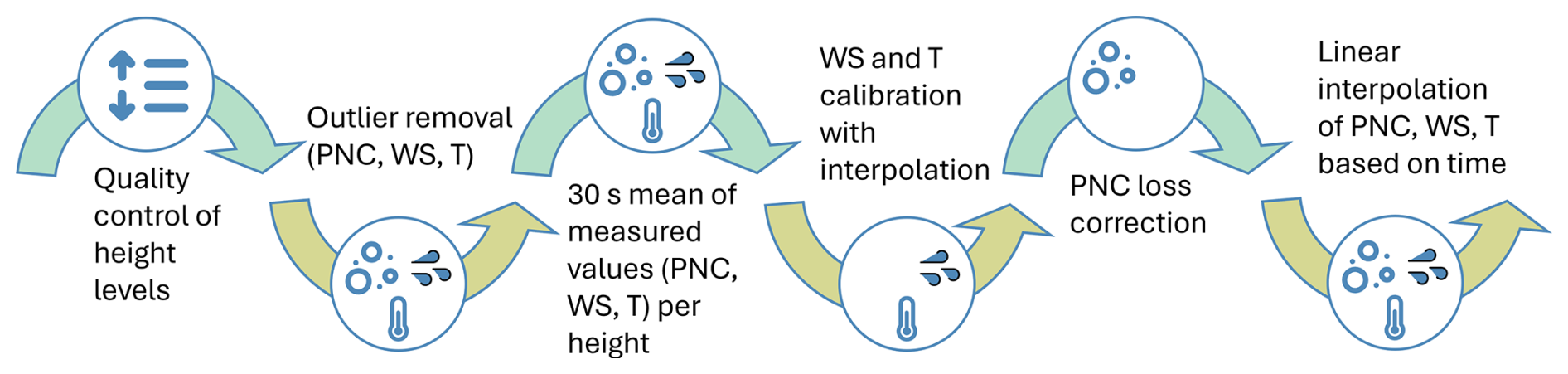
Figure A2 Step-by-step data analysis procedure for the gradient system, including temperature (T), wind speed (WS) and particle number concentration (PNC) data.

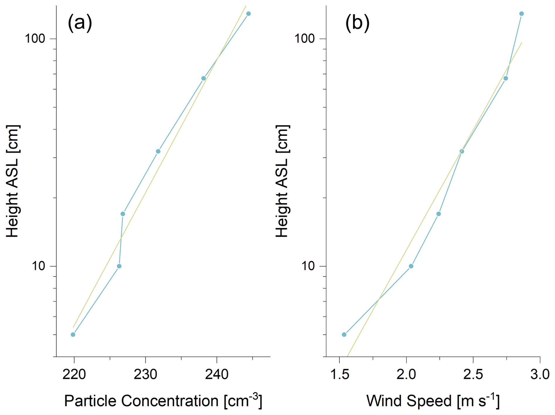
Figure A3 Example of vertical profiles of (a) particle concentration [cm⁻³] and (b) wind speed [m s⁻¹] over closed ice on 5 June 2023. The beige line shows the linear regression fit, with R²=0.98 for the particle concentration gradient and R²=0.99 for the wind speed gradient. Utilizing the calculated $u^{*}\ge \mathrm{0.15}$ m s⁻¹, a flux of 0.47 × 10⁶ m⁻² s⁻¹ was derived.

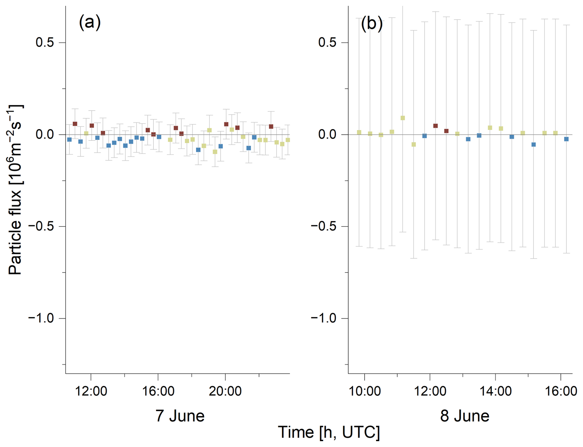
Figure A4 Particle flux [P, 10⁶ m⁻² s⁻¹] at narrow lead surface type on (a) 7 June and (b) 8 June 2023. The brown color indicates net particle emission intervals and the blue color indicates net particle deposition intervals. The beige color indicates intervals where $u^{*}<\mathrm{0.15}$ m s⁻¹. The gray-shaded bars illustrate the maximum error value for the day of measurement, as estimated by Monte Carlo simulations.

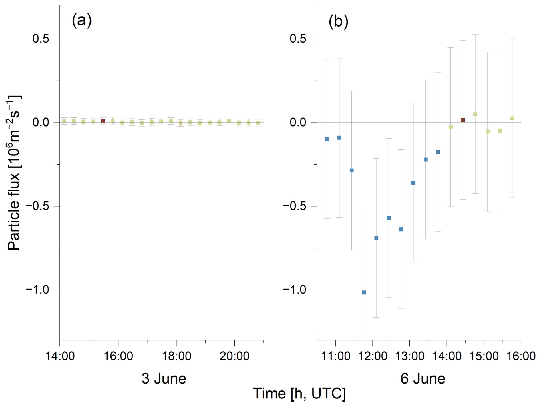
Figure A5 Particle flux [P, 10⁶ m⁻² s⁻¹] at closed ice surface type on (a) 3 June and (b) 6 June 2023. The brown color indicates net particle emission intervals and the blue color indicates net particle deposition intervals. The beige color indicates intervals where $u^{*}<\mathrm{0.15}$ m s⁻¹. The gray-shaded bars illustrate the maximum error value for the day of measurement, as estimated by Monte Carlo simulations.

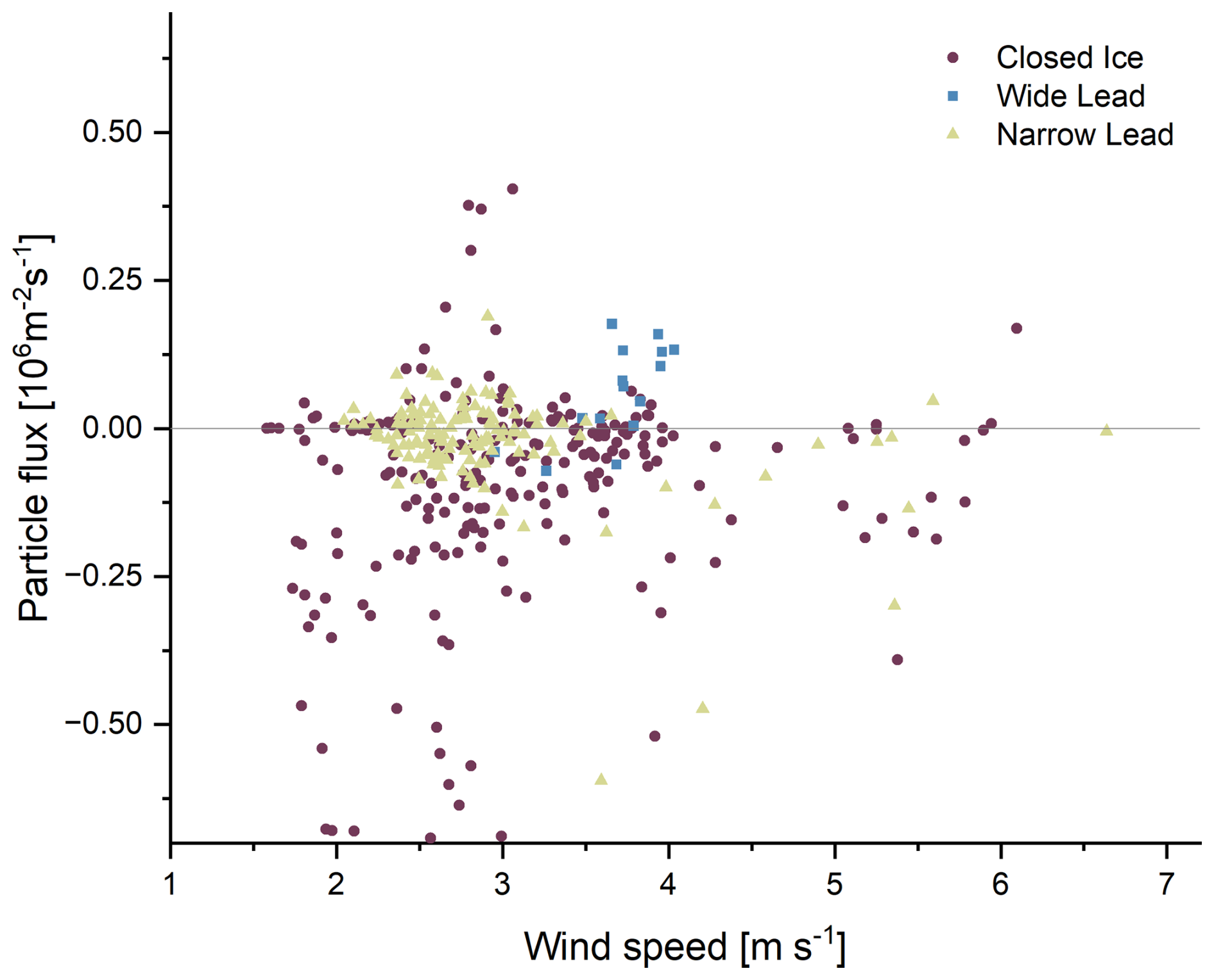
Figure A6 Particle flux [P, 10⁶ m⁻² s⁻¹] and wind speed [m s⁻¹] at the three surface types, closed ice, wide lead and narrow lead, for the entire measurement period.