Polar winter climate change: strong local effects from sea ice loss, widespread consequences from warming seas

Decreasing sea ice cover and warming sea surface temperatures (SSTs) impact the climate at both poles in uncertain ways. We aim to reduce the uncertainty by comparing output of 41-year-long simulations from four atmospheric general circulation models (AGCMs). In our “Baseline” simulations, the models use identical prescribed SSTs and sea ice cover conditions representative of 1950–1969. In three sensitivity experiments, the SSTs and sea ice cover are individually and simultaneously changed to conditions representative of 2080–2099 in a strong warming scenario. Overall, the models agree that warmer SSTs have a widespread impact on 2 m temperature and precipitation, while decreasing sea ice cover mainly causes a local response (i.e. the greatest warming occurs where sea ice is perturbed). Thus, decreasing sea ice cover causes greater changes in precipitation and temperature than in warmer SSTs in areas where sea ice cover is reduced, while warmer SSTs dominate the response elsewhere. In general, the response in temperature and precipitation to simultaneous changes in SSTs and sea ice cover is approximately equal to the sum due to individual changes, except in areas of sea ice decrease where the joint effect is smaller than the sum of the individual effects. The models agree less well on the magnitude and spatial distribution of the response in mean sea level pressure; i.e. uncertainties associated with atmospheric circulation responses are greater than uncertainties associated with thermodynamic responses. Furthermore, the circulation response to decreasing sea ice cover is sometimes significantly enhanced but sometimes counteracted by the response to warmer SSTs.

1 Introduction

Dramatic sea ice loss has been recorded at both poles during the last decade (Parkinson, 2019, 2022). The reduction in sea ice is most pronounced in the Arctic, where the surface has warmed nearly 4 times faster than the global average over the past 45 years (Rantanen et al., 2022). The rate and magnitude of sea ice loss are projected to continue at both poles – they may even increase if there are no drastic cuts in greenhouse emissions (IPCC, 2022). This transition in polar climates can potentially affect weather patterns across the whole globe (Cohen et al., 2014; Vihma, 2014; England et al., 2020; Tewari et al., 2023) and will without a doubt have significant consequences for people living within or near the polar regions.

Earth system models (ESMs) and atmospheric general circulation models (AGCMs) agree on many general features of a warmer future Arctic and Antarctic, but they strongly disagree on critical details, such as the exact magnitude of the warming and sea ice reduction rates (Stuecker et al., 2018; Han et al., 2023). These discrepancies may influence our understanding of how changes in sea ice affect circulation patterns and weather systems within and outside the polar regions (Smith et al., 2022). Polar warming rates depend on local feedback processes (e.g. changes in clouds, precipitation, sea ice extent) as well as changes in remote drivers (e.g. oceanic and atmospheric heat transport), which are both highly uncertain (Lenaerts et al., 2017; Wendisch et al., 2019; Kim and Kim, 2018; Cronin et al., 2017). Several studies have pointed out the importance of better understanding local feedbacks in polar regions, in particular related to clouds, for better constraining the magnitude of polar amplification and ice melt (Screen et al., 2018; Kittel et al., 2022; Ryan et al., 2022).

To address the issues outlined above, we have designed and executed a set of coordinated simulations with four different AGCMs. The idealized simulations have been performed with individual and simultaneous changes in prescribed sea surface temperatures (SSTs) and sea ice cover following a future anthropogenic emission scenario. The experimental setup allows us to isolate feedbacks that are driven by either SST or sea ice cover changes and to examine the linearity of these feedbacks. Using four different AGCMs, we can also investigate the robustness of the atmospheric responses. The overall aim has been to better understand the processes that drive interactions between polar regions and lower latitudes, their structural uncertainty, and their response to local and remote forcing under changing climate conditions. An additional aim is to contribute to model development as the results are dependent on the ability of the models to describe atmospheric processes. In this paper, we describe the simulation setup and discuss some high-level results with a focus on basic meteorological variables (2 m air temperature, surface precipitation, and mean sea level pressure).

Specifically, we target the following questions.

• When models are constrained by prescribed SSTs and sea ice cover changes, do they agree on how basic meteorological parameters in the polar regions change in a warmer climate?

• How significant are inter-model differences in the simulated responses in, on the one hand, thermodynamic quantities like air temperature and, on the other hand, dynamic quantities like mean sea level pressure?

• What is the most important oceanic driver of the atmospheric responses within the polar regions and in mid-latitudes – changes in SST or sea ice cover?

Our analysis is focused on the winter season in the Arctic and Antarctic, when changes in atmospheric circulation patterns should be most prominent and the decrease in sea ice cover has the most notable impact on meteorological variables (e.g. Screen and Simmonds, 2010).

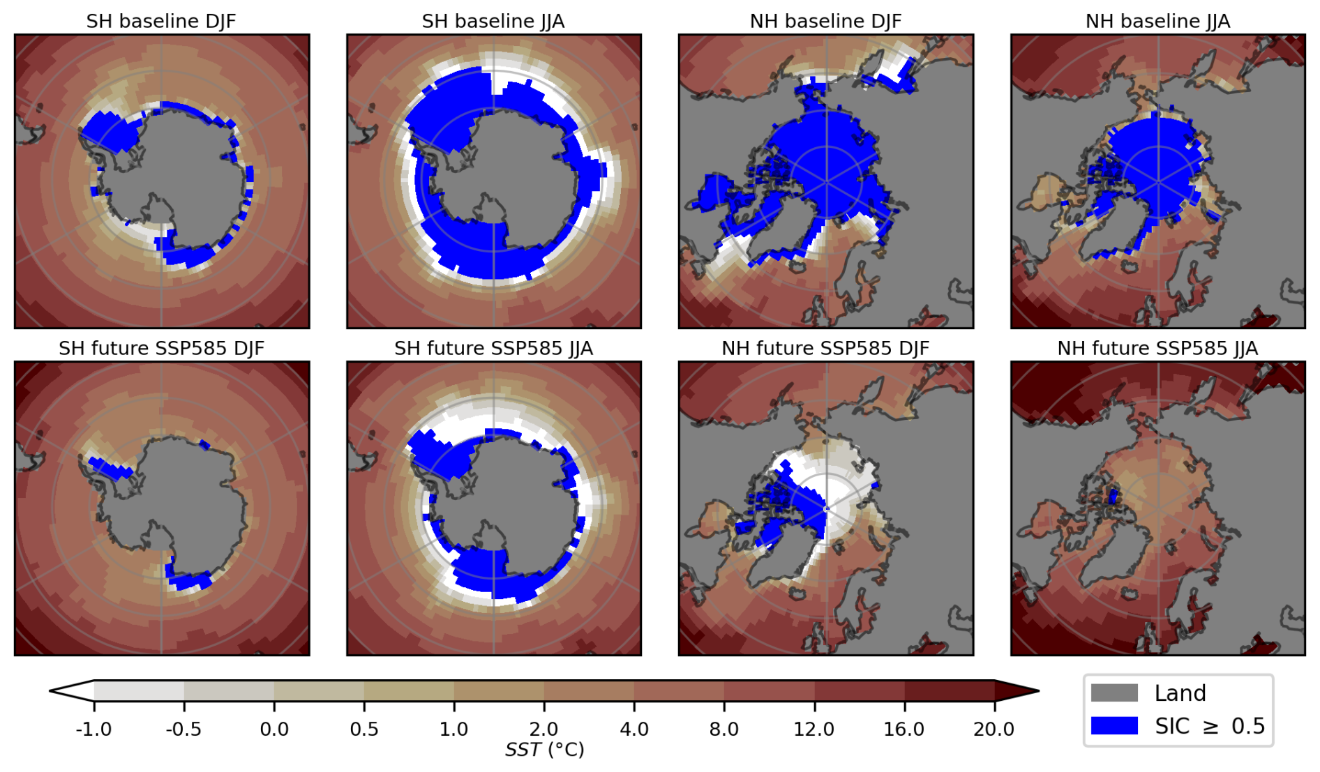
Figure 1 Winter (DJF) and summer (JJA) mean sea ice cover and sea surface temperature (SST) in the Baseline experiment (upper row) and in the SSP585 experiment (lower row).

2 Methods

2.1 Experimental setup

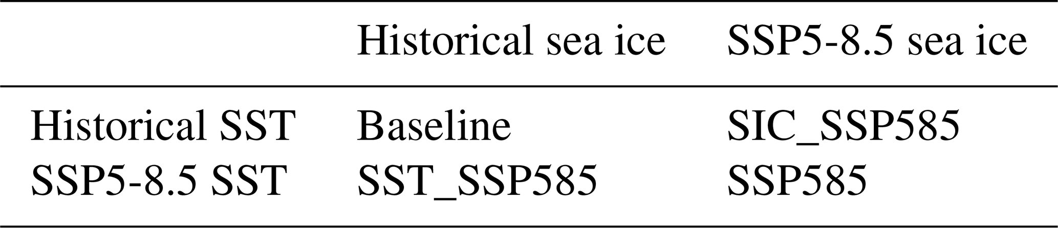
A Baseline simulation and three different perturbation experiments from four different AGCMs (see Sect. 2.2) were performed and analysed (Table 1). The experiments follow an Atmospheric Model Intercomparison Project (AMIP) configuration (Gates, 1992; Gates et al., 1999). In all experiments, we used prescribed SSTs (variable “tos”) and sea ice area fraction (variable “siconc”, hereafter referred to as “sea ice cover”) from simulations using the Australian Earth system model ACCESS-ESM1.5 (Ziehn et al., 2020, 2019a, b), available from the Coupled Model Intercomparison phase 6 (CMIP6) archive. We chose the ACCESS-ESM1.5 output for our simulations as the model produces an Arctic sea ice cover evolution for the historical period that is in reasonable agreement with observations (Notz and SIMIP Community, 2020). The model was also selected by the CMIP6 Sea-Ice Model Intercomparison Project community to estimate a best guess of the future evolution of Arctic sea ice cover (Notz et al., 2020). Monthly mean SST and sea ice cover averaged over 20 years of simulation were taken from either the historical simulation (years 1950–1969, Baseline simulation) or the SSP5-8.5 scenario simulation (years 2080–2099). In each simulation, the same annual cycle was repeated for all the 41-year simulation. A similar set of model runs was performed for the low-emissions SSP1-2.6 scenario, but in the interest of brevity, only the SSP5-8.5 results are discussed in this paper. In addition, the significant changes in sea ice cover and SST in the SSP5-8.5 scenario amplify the effects of warming, and thus the SSP5-8.5 simulation makes the signal-to-noise ratio significantly stronger than in the SSP1-2.6 scenario. SSTs and sea ice cover were linearly interpolated between each month and changed both individually and simultaneously compared to the Baseline simulation (Table 1). Note that our experimental setup is different from, for example, the Polar Amplification Model Intercomparison Project (PAMIP; Smith et al., 2019). In the PAMIP experiments, mostly short (1-year) simulations were performed with large ensembles of initial states, whereas our experiments consist of long (40-year) simulations. The PAMIP simulations address pre-industrial, present-day, and future climates, whereas our simulations focus only on differences between present-day and future climates. The changes in sea ice cover and SSTs were also substantially greater in our experiments than in the PAMIP atmosphere-only simulations. In ACCESS-ESM1.5 (i.e. the model we use for the SST and sea ice forcing fields), the global average increase in 2 m temperature between the Baseline and future period (using the SSP5-8.5 scenario) is 4.4 K, whereas the warming in the PAMIP simulations is approximately 2 K comparing future and pre-industrial conditions. In our future simulations, the Arctic Ocean is almost ice-free during the whole year (Fig. 1), which helps to boost the signal-to-noise ratio of the simulated climate responses. Another difference compared to the PAMIP experiments is that our forcing fields are based on output from only one model (ACCESS-ESM1.5), whereas PAMIP uses a combination of observations and multi-model averages.

Table 1 Name of model experiments and their respective SST and sea ice cover configuration.

Each experiment was run for 41 years, with perpetual monthly average values of SSTs and sea ice cover. All other conditions (e.g. greenhouse gas concentrations, aerosol emissions) were prescribed according to the year 2000 in all models and experiments. Each model used their default parameterizations of snow and ice albedos as well as for natural aerosols (see Sect. 2.2). The first year of simulation was considered as a spin-up and discarded from the analysis, leaving 40 years of output for analysis. In the simulations where only the sea ice cover was changed (i.e. SIC_SSP585), the SSTs were kept at their Baseline values. This means that the surface temperature is reduced slightly over areas where sea ice is removed since the temperature of the sea ice–ocean water interface is slightly lower than the melting point of freshwater. Based on our simulations, the total climate response (ΔX_full) for any given variable caused by the use of future boundary conditions (SSP5-8.5) compared to the Baseline can be decomposed into three parts:

$$\begin{array}{}\text{(1)}& \mathrm{\Delta }{X}_{\text{full}}=\mathrm{\Delta }{X}_{\text{SST}}+\mathrm{\Delta }{X}_{\text{SIC}}+\mathrm{\Delta }{X}_{\text{NL}},\end{array}$$

where X is any climate variable (e.g. temperature or precipitation), ΔX_SST is the contribution from the SST change, ΔX_SIC is the contribution from the sea ice cover change, and ΔX_NL is the non-linear (or residual) contribution:

$$\begin{array}{}\text{(2)}& {\displaystyle }\mathrm{\Delta }{X}_{\text{full}}=X_{\text{SSP585}}-X_{\text{Baseline}}\text{(3)}& {\displaystyle }\mathrm{\Delta }{X}_{\text{SST}}=X_{\text{SST\hspace{0.17em}SSP585}}-X_{\text{Baseline}}\text{(4)}& {\displaystyle }\mathrm{\Delta }{X}_{\text{SIC}}=X_{\text{SIC\hspace{0.17em}SSP585}}-X_{\text{Baseline}}\text{(5)}& {\displaystyle }\mathrm{\Delta }{X}_{\text{NL}}=\mathrm{\Delta }{X}_{\text{full}}-\mathrm{\Delta }{X}_{\text{SST}}-\mathrm{\Delta }{X}_{\text{SIC}}.\end{array}$$

2.2 Models

Three ESMs (CESM2, NorESM2, and EC-Earth3) and one AGCM (OpenIFS) were used in the study. The selection of models allows us to compare differences between models belonging to the same as well as to different model families. CESM2 and NorESM2 are based on the same dynamical core but differ for some parametrizations of physical processes. Similarly, EC-Earth3 and OpenIFS belong to the same model family. Our model selection is also affected by the fact that the study is part of the CRiceS project (Climate Relevant interactions and feedbacks: The key role of sea ice and Snow in the polar and global climate system), which aims to improve the description of polar atmospheric processes in ESMs, in particular NorESM2 and EC-Earth3. Below we provide a brief description of the models. We only describe the atmospheric part of each model since we use prescribed SSTs and sea ice cover in all simulations. Note that the different model components were connected to each other through radiative heat fluxes, sensible and latent heat fluxes, and momentum fluxes during the simulations, but the ocean and sea ice components were not utilized for predicting the evolution of sea ice or SSTs (since these were prescribed in the experiments). In other words, the sea ice model was only utilized to compute, for example, the surface temperature of sea ice and the surface fluxes between the atmosphere and sea ice. The surface albedo, including the effects of snow, was computed within the sea ice and land components.

2.2.1 CESM2

The atmospheric component of the community Earth system model version 2 (CESM2) is the Community Atmosphere Model version 6 (CAM6; Danabasoglu et al., 2020). CAM6 is based on a hydrostatic finite-volume dynamical core with a regular latitude–longitude grid. The horizontal resolution of CAM6 is 1.25°×0.9° (long×lat) and the model has 32 vertical levels up to 2.3 hPa. The aerosol module is the Modal Aerosol Model version 4 (MAM4; Liu et al., 2016), and aerosols are interactive with clouds. Radiative transfer is modelled using the Rapid Radiative Transfer Model for General circulation models (RRTMG; Danabasoglu et al., 2020). Cloud microphysics follows a two-moment scheme with four hydrometeor species (cloud water, cloud ice, rain, and snow) (Gettelman and Morrison, 2015), and mixed-phase clouds can occur in the temperature range 0 to −37 °C (Gettelman et al., 2010). The other model components in CESM2 are the Community Land Model 5.0 (CLM5) for land processes and interactions between the land and atmosphere, the Model for Scale Adaptive River Transport (MOSART) for river runoff, the Community Ice CodE (CICE) for sea ice, SWAV for oceanic waves, and the Community Ice Sheet Model (CISM) for land ice.

2.2.2 NorESM2

The Norwegian Earth System Model version 2 (NorESM2; Seland et al., 2020) originates from CESM2. NorESM2 thus has many model components that are the same as in CESM2. The main difference is that CAM6 has been replaced by CAM6-Nor. In addition, the land ice and ocean wave components have not been used in the NorESM2 experiments. CAM6-Nor uses the same cloud and radiation schemes as CAM6. The greatest differences between CAM6 and CAM6-Nor are associated with the aerosol physics and aerosol–cloud–radiation interactions (Seland et al., 2020; Kirkevåg et al., 2013, 2018). For the current study, we use the low-resolution model version of NorESM2, which has a horizontal resolution of 2.5°×1.9° (long×lat) and the same vertical levels as CESM2.

The evolution of different aerosol particle types is described with the NorESM2 aerosol scheme. Aerosol particles interact with clouds, affecting, for example, cloud droplet activation and the freezing of cloud droplets (Storelvmo et al., 2006). The formation of ice crystals may occur due to heterogeneous nucleation and heterogeneous freezing where mineral dust and black carbon can act as ice-nucleating particles (Kirkevåg et al., 2018).

2.2.3 OpenIFS

OpenIFS is a research model built from the Integrated Forecast System (IFS), the operational numerical weather prediction (NWP) model from the European Centre for Medium-Range Weather Forecasts (ECMWF). We have used the version 43r3 of OpenIFS (hereafter referred to as OpenIFS), which is derived from IFS CY43R3 (used for operational forecasting at ECMWF from July 2017 to June 2018). The dynamical core uses spectral semi-Lagrangian and semi-implicit methods. The experiment configuration uses spectral linear truncation TL255 (approx. 80 km at the Equator) as a horizontal resolution and 91 hybrid model levels up to 0.01 hPa.

The version of OpenIFS used does not include interactive aerosols. The radiation scheme uses global aerosol fields from monthly climatological means produced by the Copernicus Atmospheric Monitoring Service. Cloud condensation nuclei concentrations are prescribed as one constant value over land and ocean, respectively. The exact implementation is described in Bozzo et al. (2017).

The OpenIFS one-moment cloud scheme contains six moisture-related prognostic variables (water vapour, cloud water, cloud ice, cloud fraction, rain, and snow). The prognostic cloud fraction and sources and sinks for cloud variables are calculated from the major generation and destruction processes. The separate treatment for cloud water and cloud ice allows for the representation of supercooled liquid and mixed-phase clouds (ECMWF, 2014). The radiation processes of OpenIFS 43r3 are handled by the ecRad scheme (Hogan and Bozzo, 2018).

The land surface scheme in OpenIFS is handled by the Hydrology Tiled ECMWF Scheme for Surface Exchanges over Land (HTESSEL; Balsamo et al., 2009), which also handles surface fluxes due to sea surface temperature and sea ice, which are controlled by the experiments described above. Furthermore, OpenIFS includes an ocean surface wave model, which couples the wind–wave interaction and calculates the kinematic part of the energy balance equation over the ocean.

OpenIFS is primarily intended as a model for NWP. Nevertheless, configurations for nudged or free-run simulation are implemented. The free-run configuration has been used in the present study, in tandem with in-built fixers for global mass and moisture to produce atmosphere-only climate simulation.

2.2.4 EC-Earth3

The EC-Earth3 experiments were carried out with EC-Earth3-AerChem version 3.3.4.1 (van Noije et al., 2021; Döscher at al., 2022), which is the model configuration with interactive aerosols and atmospheric chemistry used in the Aerosol and Chemistry Model Intercomparison Project (AerChemMIP). The atmospheric component of EC-Earth3 is based on the ECMWF IFS CY36R4, which was operational from November 2010 to May 2011. Land surface processes are simulated with HTESSEL. The cloud scheme in EC-Earth3 is the same as in OpenIFS, but there are differences in the treatment of other physical processes, including convection, and radiation is parameterized with the McRad scheme (Morcrette et al., 2008). Aerosols and chemical processes in the atmosphere are described by the chemical transport tracer model version 5 (TM5) (van Noije et al., 2014). Tropospheric aerosols influence the cloud droplet number concentration but not the ice number concentrations. The spatial discretization of the atmospheric model was the same as for OpenIFS – that is, TL255 in the horizontal and 91 levels in the vertical, while TM5 was run at a lower resolution of 3°×2° (long×lat), with 34 vertical levels and a top at 0.1 hPa.

3 Results

The experiments targeting our science questions were not covered by the CMIP6 protocol; therefore, we use the specific model protocol defined in Sect. 2.1. Given this, our results cannot be directly compared with the historical and future scenario (SSP5-8.5) simulations. Most importantly, we use prescribed SSTs and sea ice cover from one specific model (ACCESS-ESM1.5), and we also apply constant greenhouse gas concentrations (for the year 2000) in all simulations. Nevertheless, in Sect. 3.1 we compare our Baseline and SSP_585 experiments with the historical (years 1950–1969) and scenario SSP5-8.5 (years 2080–2099) experiments from CMIP6 to put our simulation results into the context of these simulations. In Sect. 3.2 and 3.3, we thereafter examine the future climate response in the Antarctic and Arctic, respectively, by comparing our future simulations (SSP585, SST_SSP585, SIC_SSP585) with the Baseline (see Table 1). In the analysis, we focus on the winter seasons in both hemispheres and start our analysis with the Antarctic region, which has received less attention than the Arctic in previous research.

3.1 Comparison with CMIP6 models

Figures 2 and S1 in the Supplement show that our Baseline and SSP585 simulations agree well with the corresponding CMIP6 simulations for several key climate variables, even though the boundary conditions are slightly different. The simulated zonal mean 2 m temperature, mean sea level pressure (MSLP), and precipitation are within the range of the minimum and maximum of the 23 CMIP6 models, and they are also generally close to the CMIP6 multi-model mean (Figs. 2 and S1). This result indicates that our simulations reproduce the general features of the historical and future (SSP5-8.5) climate conditions, as modelled by CMIP6.

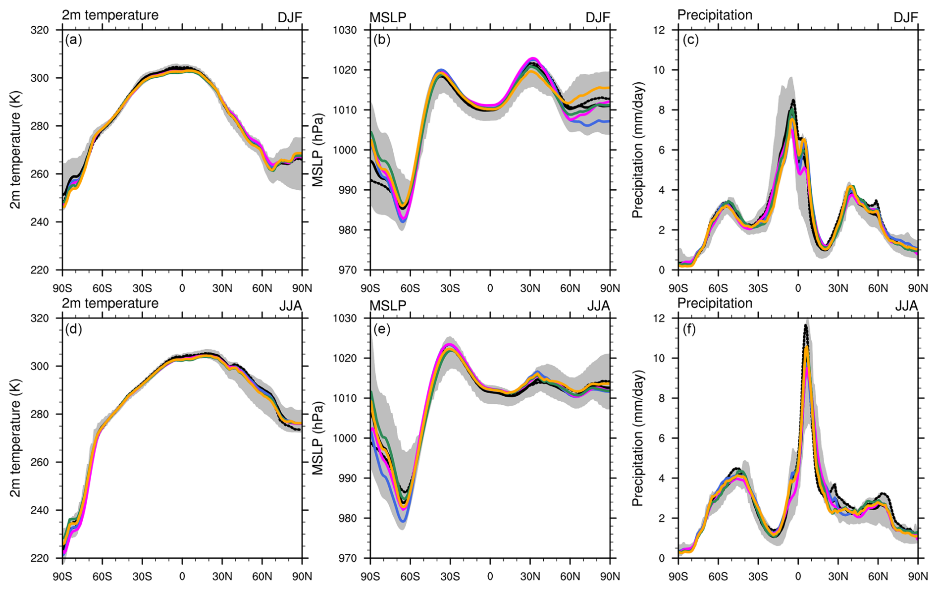
Figure 2 Seasonal means of zonal mean 2 m temperature (left, a, d), mean sea level pressure (middle, b, e), and precipitation (right, c, f), in the Baseline simulations and in the CMIP6 historical simulations (years 1950–1969). The blue (CESM2), magenta (NorESM2), green (EC-Earth3), and yellow (OpenIFS) lines show the models applied in the present study; the solid black line shows the CMIP6 multi-model mean; and the dashed black line shows the ACCESS-ESM1.5 CMIP6 simulation where sea ice cover and SST were taken. The grey area shows the range between the minimum and maximum of the 23 CMIP6 models. The upper row (a–c) shows the mean values for the Northern Hemisphere winter (DJF), and the lower row (d–f) shows the mean values for the Southern Hemisphere winter (JJA).

In the Baseline simulation, the greatest deviations from the CMIP6 multi-model mean 2 m temperature occur at the winter poles, where our models are generally warmer than the CMIP6 multi-model mean (Fig. 2a and d). This difference may be associated with the different greenhouse gas and aerosol concentrations applied in the present study (which are from the year 2000). However, the simulated 2 m temperatures in our SSP585 simulations and the differences between our Baseline and SSP585 simulations are in general close to the CMIP6 SSP5-8.5 multi-model mean and the differences between corresponding CMIP6 historical and CMIP6 SSP5-8.5 simulations (Figs. S1 and S2), despite the differences in greenhouse gas and aerosol concentrations. The greatest MSLP deviations from the CMIP6 multi-model mean also occur in the polar regions (Fig. 2b and e). In particular, CESM2 and NorESM2 have a deeper circumpolar trough and a stronger subtropical high over the Southern Hemisphere, suggesting stronger westerly winds over the Southern Ocean. In terms of precipitation, our model simulations agree well with the CMIP6 multi-model mean (Fig. 2c and f).

3.2 Antarctic

3.2.1 Temperature

As an average over the Antarctic (60–90°), the models agree on the changes in 2 m temperature, both when SST and sea ice cover are changed jointly and when they are changed individually (Fig. 3a). The increase in SSTs and the decrease in sea ice cover cause on average an almost equal change in wintertime (JJA) 2 m temperature in the southern polar region. The greatest increase in 2 m temperature between SSP585 and Baseline (ΔT_full) occurs over the Southern Ocean, around the Antarctic continent where the sea ice has been removed (up to 11 K, Fig. 4a). The 2 m temperature increases significantly also over the Antarctic continent, but the increase is smaller, mostly 4–5 K. The models generally agree on the warming pattern (Fig. S3), but there are quantitative differences (Fig. 4e). These are in general spatially correlated with the strength of warming, except over the Weddell Sea, where the strongest warming over the Antarctic region occurs and the differences between the models are small.

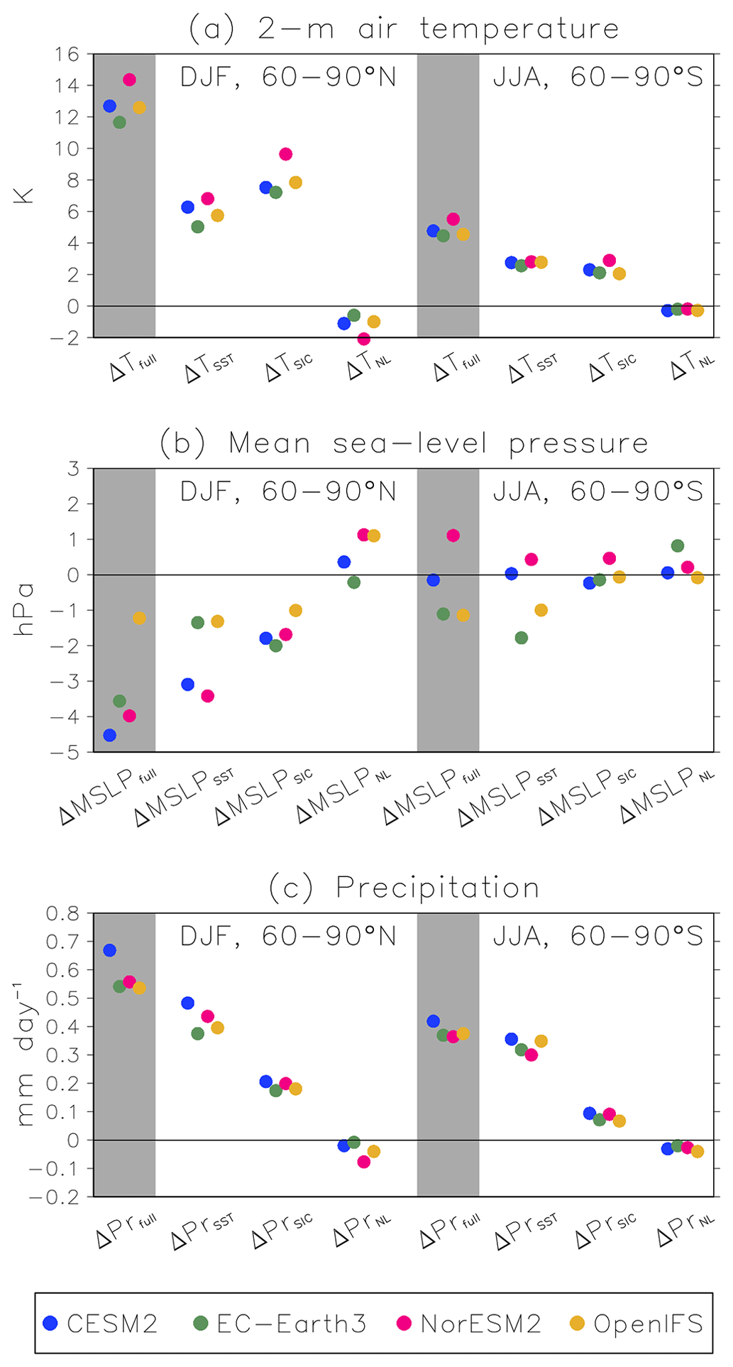
Figure 3 Area mean differences between the SSP585 simulation and Baseline (ΔX_full, grey shading), between SIC_SSP585 and Baseline (ΔX_SIC), between SST_SSP585 and Baseline (ΔX_SST), and the non-linear (residual) contribution (ΔX_NL) for the northern high latitudes (left) (60–90° N) in the Northern Hemisphere winter (DJF) and the southern high latitudes (right) (60–90° S) in the Southern Hemisphere winter (JJA) for (a) 2 m temperature, (b) mean sea level pressure, and (c) precipitation.

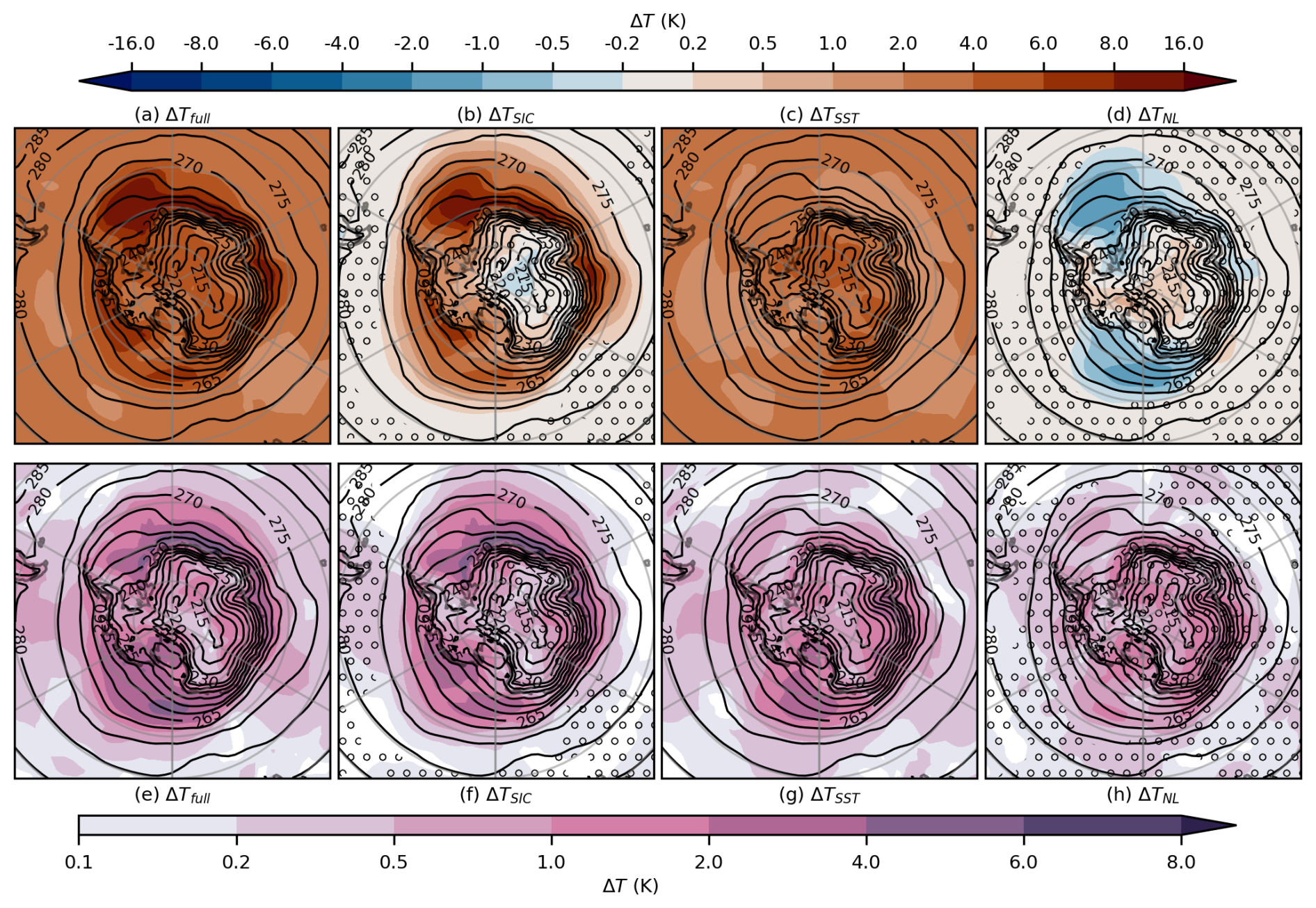
Figure 4 Difference in 2 m temperature (T) in austral winter (JJA) between the SSP585 simulation and Baseline (ΔT_full, a, e), between SIC_SSP585 and Baseline (ΔT_SIC, b, f), between SST_SSP585 and Baseline (ΔT_SST, c, g), and the non-linear (ΔT_NL residual) contribution (d, h). The upper row (a–d) shows the multi-model mean, and the lower row (e–h) shows the maximum difference between models. Stippling indicates that all models do not agree on the direction of the change, and contours show the 2 m temperature in the Baseline simulation.

The warming over regions that originally had sea ice is predominantly driven by decreases in sea ice cover (ΔT_SIC, Fig. 4b), whereas the warming over the continent and ice shelves is mainly caused by warmer SSTs (ΔT_SST, Fig. 4c). Over the continent, ΔT_SIC is weak or even negative. The difference in 2 m temperature between SSP585 and Baseline (ΔT_full) is on average close to the sum of the individual changes due to increased SSTs (ΔT_SST) and decreased sea ice cover (ΔT_SIC), except in the areas where the decrease in sea ice cover causes the most significant warming, i.e. the Weddell Sea, the D'Urville Sea, and the Ross Sea (non-stippled ocean regions in Fig. 4h). In these areas, the models agree that the sum of ΔT_SST and ΔT_SIC is greater than ΔT_full. Overall, the models also agree on the warming patterns due to warmer SSTs and decreased sea ice cover.

3.2.2 Mean sea level pressure

The models do not agree on the average change in MSLP (ΔMSLP_full) over the Antarctic region: NorESM2 shows a positive ΔMSLP_full on average, and EC-Earth3 and OpenIFS show that the average ΔMSLP_full is negative, whereas the average ΔMSLP_full is small in CESM2 (Fig. 3b). The multi-model mean ΔMSLP_full is positive over the Pacific sector between 50 and 70° S and over the Atlantic sector northward of 60° S. In contrast, there is a decrease in MSLP on the Australian side of the Southern Ocean, near the Antarctic coast and over the Weddell Sea (Fig. 5a). However, all models do not agree on the regional pattern of MSLP changes. OpenIFS does not show an increase in MSLP over the Pacific sector, and the maximum decrease in MSLP on the Australian side of the Southern Ocean is also located slightly to the west of the maxima of the other models (Fig. S4). The multi-model mean changes in MSLP indicate a weakening of the Amundsen low, while cyclones over the Australian side of the Southern Ocean most likely become deeper or more frequent (or blockings become more infrequent). In addition, a poleward shift of the circumpolar trough, especially in the Atlantic sector, indicates a more positive southern annular mode (SAM), which suggests stronger westerly winds at mid-latitudes and more cyclones near the Antarctic coast.

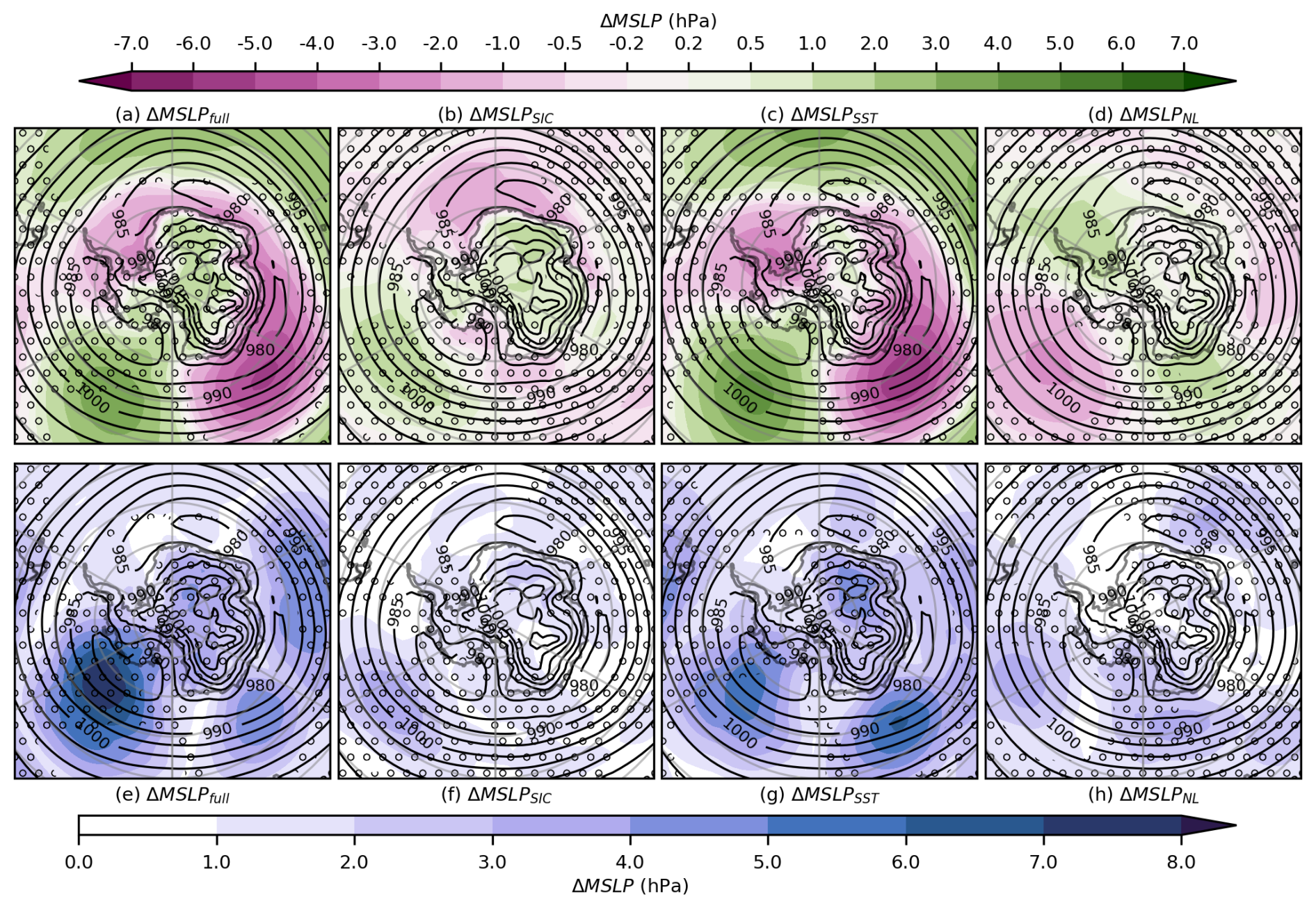
Figure 5 Difference in mean sea level pressure (MSLP) in austral winter (JJA) between the SSP585 simulation and Baseline (ΔMSLP_full, a, e), between SIC_SSP585 and Baseline (ΔMSLP_SIC, b, f), between SST_SSP585 and Baseline (ΔMSLP_SST, c, g), and the non-linear (ΔMSLP_NL residual) contribution (d, h). The upper row (a–d) shows the multi-model mean, and the lower row (e–h) shows the maximum difference between models. Stippling indicates that all models do not agree on the direction of the change, and contours show MSLP in the Baseline simulation.

The changes in MSLP are mostly driven by warmer SSTs (ΔMSLP_SST, Fig. 5c), while the decrease in sea ice cover (ΔMSLP_SIC, Fig. 5b) causes a much weaker response. The models mostly disagree on the direction of the change (stippling in Fig. 5b) except over the Weddell Sea (where all models indicate a decrease in MSLP) and over the central continent (where all models indicate an increase in MSLP). In some regions, the changes in MSLP due to the decrease in sea ice cover are opposite in sign compared to those driven by the SSTs. Even though the models mostly disagree on the direction of the non-linear change in MSLP (ΔMSLP_NL), they agree that there is a decrease in MSLP in the Amundsen Sea and an increase in MSLP in the Pacific sector of the Southern Ocean (Fig. 5d). The multi-model mean of ΔMSLP_NL is mainly opposite to the multi-model mean of ΔMSLP_full, suggesting that the sum of the individual responses to changes in SST and sea ice cover overestimates the full response.

3.2.3 Precipitation

All models show a general increase in precipitation (ΔPr_ful) over the southern polar region (Fig. 3c), with a similar regional pattern in all models (Fig. S5). The greatest absolute increase in precipitation occurs over the Southern Ocean, especially in its Australian sector, where the decrease in MSLP is strongest (Fig. 6a). However, the relative increases are greater over the continent and coastal areas, where there is up to twice as much precipitation in SSP585 compared to Baseline (Fig. S6). Three (CESM2, NorESM2, and EC-Earth3) out of four models indicate that the greatest relative increase in precipitation occurs over the continent west of the Ross Sea. These models also show negative or very small positive changes in precipitation in the coastal areas between the longitudes of the Indian Ocean side of the Antarctic (90–120° E; right-hand side of the figure panels). The dipole structure in the MSLP changes over the Pacific sector (Fig. 5a) and is strongest in these models, indicating that these changes in precipitation are, at least partly, driven by changes in circulation.

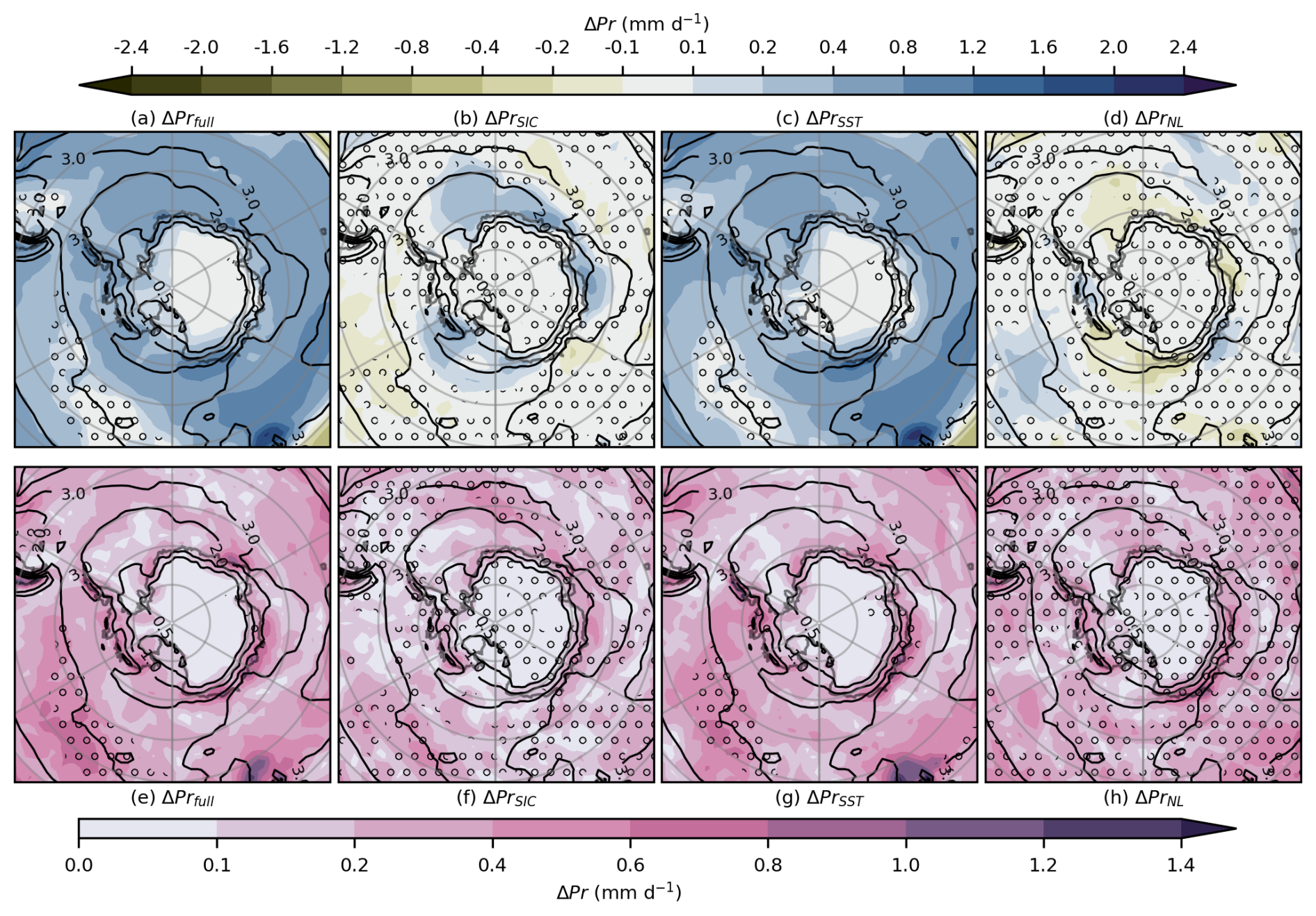
Figure 6 Difference in precipitation (Pr) in austral winter (JJA) between the SSP585 simulation and Baseline (ΔPr_full, a, e), between SIC_SSP585 and Baseline (ΔPr_SIC, b, f), between SST_SSP585 and Baseline (ΔPr_SST, c, g), and the non-linear (ΔPr_NL residual) contribution (d, h). The upper row (a–d) shows the multi-model mean, and the lower row (e–h) shows the maximum difference between models. Stippling indicates that all models do not agree on the direction of the change, and contours show precipitation in the Baseline simulation.

All models agree that the increase in precipitation is mostly driven by increased SSTs (ΔPr_SST, Figs. 3c and 6c), while the decrease in sea ice cover (ΔPr_SIC, Fig. 6b) mainly causes small increases in precipitation over the areas where sea ice cover is reduced. The increase in precipitation due to a sea ice decrease (ΔPr_SIC) is collocated with the areas where evaporation increases (Fig. S14), suggesting that increased evaporation increases precipitation locally, potentially due to enhanced shallow convection associated with cold air outbreaks. In addition, ΔPr_SIC is relatively significant over the coastal areas, suggesting that enhanced evaporation increases the amount of water vapour in air masses advected to the continent.

3.3 Arctic

3.3.1 Temperature

In the Arctic, the increase in 2 m temperature due to simultaneous changes in SST and sea ice (on average ∼13 K) is substantially greater than in the Antarctic (on average ∼5 K, Fig. 3a). In the Northern Hemisphere winter, the greatest increases in 2 m temperature between SSP585 and Baseline (ΔT_full) are found over the Arctic Ocean, Siberia, and the Canadian Arctic Archipelago (Fig. 7a). All models agree on the general pattern of warming, but there are significant absolute differences around northern Greenland and over the Canadian Arctic Archipelago and in Siberia (Fig. 7e). Over Siberia, CESM2 and NorESM2 simulate stronger warming than EC-Earth3 and OpenIFS (Fig. S7). Overall, OpenIFS shows the weakest warming over the continents, whereas NorESM2 shows the strongest warming.

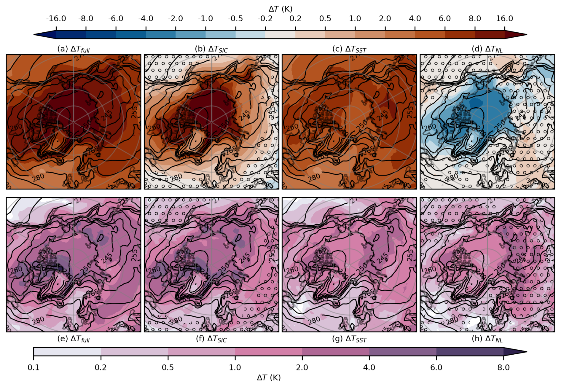
Figure 7 Difference in 2 m temperature (T) in winter (DJF) between the SSP585 simulation and Baseline (ΔT_full, a, e), between SIC_SSP585 and Baseline (ΔT_SIC, b, f), between SST_SSP585 and Baseline (ΔT_SST, c, g), and the non-linear (ΔT_NL residual) contribution (d, h). The upper row (a–d) shows the multi-model mean, and the lower row (e–h) shows the maximum difference between models. Stippling indicates that all models do not agree on the direction of the change, and contours show the 2 m temperature in the Baseline simulation.

The decrease in sea ice (ΔT_SIC, Figs. 3a and 7b) produces on average greater warming than the increase in SSTs (ΔT_SST, Fig. 7c) in the northern polar region, especially over the Arctic Ocean and in the Canadian Arctic Archipelago. There, the multi-model mean ΔT_SIC reaches 22 K locally, which is substantially greater than the maximum ΔT_SIC in the Antarctic region (∼10 K, Fig. 4b). In general, the decrease in sea ice cover mainly has a local effect on the 2 m temperature; i.e. the most significant changes occur in the areas or vicinity of the regions where the sea ice cover has decreased, including the coldest areas around the Arctic Ocean, such as northern Canada and Siberia. The notable increase in 2 m temperature over the continents in SIC_SSP585 is most likely due to the different characteristics of the advected air masses from the Arctic Ocean; in Baseline, the Arctic Ocean is ice-covered, whereas it is ice-free in SIC_SSP585. The relatively warm air masses do not reach far inland as the strong warming occurs mostly along the coast. Over the other areas of the Arctic, particularly the continents, ΔT_SST is greater than ΔT_SIC, indicating again that the remote effects of SST changes are important for polar continental warming. In areas where both the sea ice decrease and the SST increase cause notable warming, i.e. over the Arctic Ocean and in northern Canada, all models indicate a strong non-linearity in the 2 m temperature changes, so that the sum of ΔT_SST and ΔT_SIC is substantially greater than ΔT_full (see Discussion in Sect. 4).

3.3.2 Mean sea level pressure

The MSLP response to a simultaneous increase in SSTs and a decrease in sea ice cover (ΔMSLP_full, Fig. 8a) is more variable between the individual models than the 2 m temperature response. All models agree on an MSLP decrease near the Bering Strait, suggesting a northward shift and the strengthening of the Aleutian low. They also agree that the MSLP decreases in the central Arctic and continental Canada. In contrast, the models disagree on the changes in MSLP over the Atlantic sector. Three out of four models (CESM2, NorESM2, and EC-Earth3) indicate a decrease in MSLP over the Norwegian and Barents seas, suggesting an eastward extension of the Atlantic storm track, whereas OpenIFS shows an increase in MSLP in the same areas, suggesting a weakening of the Atlantic storm track (Fig. S8).

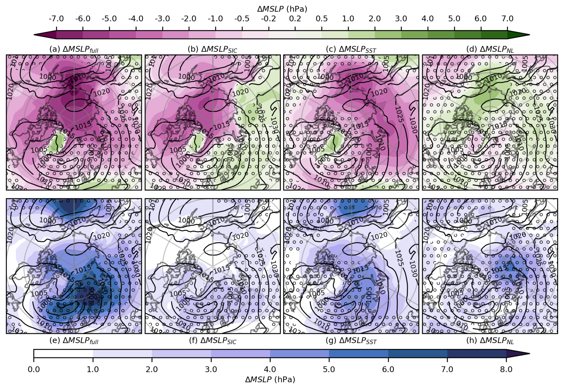
Figure 8 Difference in mean sea level pressure (MSLP) in winter (DJF) between the SSP585 simulation and Baseline (ΔMSLP_full, a, e), between SIC_SSP585 and Baseline (ΔMSLP_SIC, b, f), between SST_SSP585 and Baseline (ΔMSLP_SST, c, g), and the non-linear (ΔMSLP_NL residual) contribution (d, h). The upper row (a–d) shows the multi-model mean, and the lower row (e–h) shows the maximum difference between models. Stippling indicates that all models do not agree on the direction of the change, and contours show the MSLP in the Baseline simulation.

The models agree somewhat better on the MSLP response pattern to individual increases in SST (ΔMSLP_SST, Fig. 8g) and to decreases in sea ice cover (ΔMSLP_SST, Fig. 8f) than the full response in MSLP (Fig. 8e). In all models, a decrease in sea ice cover causes an MSLP decrease on the Canadian side of the Arctic Ocean and over the Bering Strait (Fig. 8b). However, the models disagree on the MSLP responses to decreased sea ice cover over northern Europe, where OpenIFS indicates an increase in MSLP, whereas the other models show only small changes in this region (Fig. S8). Increasing SSTs cause a decrease in MSLP over Siberia, the Siberian side of the Arctic Ocean, and the Bering Strait region in all models. However, over the northern Atlantic region, the models disagree on the direction of the MSLP changes (Fig. 8g). The non-linearities (ΔMSLP_NL, Fig. 8d) are typically smaller than the changes due to the individual forcings.

3.3.3 Precipitation

All models agree that the precipitation in the Arctic increases with warmer SSTs and a decrease in sea ice cover (ΔPr_full, Figs. 3a and 9a). The models also agree on the regional pattern of precipitation change. Most of the precipitation increase is caused by warmer SSTs (ΔPr_SST, Fig. 9c), and ΔPr_SST is greater over the ocean than over land, especially in the areas where the precipitation is strongest climatologically, i.e on the eastern side of the Atlantic and Pacific oceans. This suggests that the precipitation changes are mainly driven by the increase in atmospheric water vapour content (due to the warmer temperatures that increase the water-vapour-holding capacity of the air) rather than changes in circulation. In the northern Atlantic, south-east of Greenland, a local decrease in SSTs causes a decrease in precipitation, which also indicates a strong local effect of SST on precipitation. However, the greatest relative changes occur in the Arctic Ocean, where the increase in precipitation is at some locations more than twice the original precipitation. Furthermore, over the continents, the relative precipitation increase is greater than over the ocean. Decreasing sea ice cover mainly increases precipitation over the Arctic Ocean. This local response is associated with increased evaporation (Fig. S15), warmer surface air, and less stable stratification, which leads to convective precipitation over the Arctic Ocean during cold air outbreaks from continents (not shown). The joint effect of a decrease in sea ice cover and an increase in SST on precipitation is mostly a linear combination of the individual responses, and the residuals (ΔPr_NL, Fig. 9d) are thus mostly small. The models agree on the main changes in precipitation, i.e. an increase in precipitation in the Arctic Ocean due to a decrease in sea cover and an overall increase in precipitation due to an increase in SST. However, there are quantitative differences between the models regarding increases in precipitation (Figs. 9e–h and S9). Spatially, the differences between models are correlated with the strength of the precipitation increase.

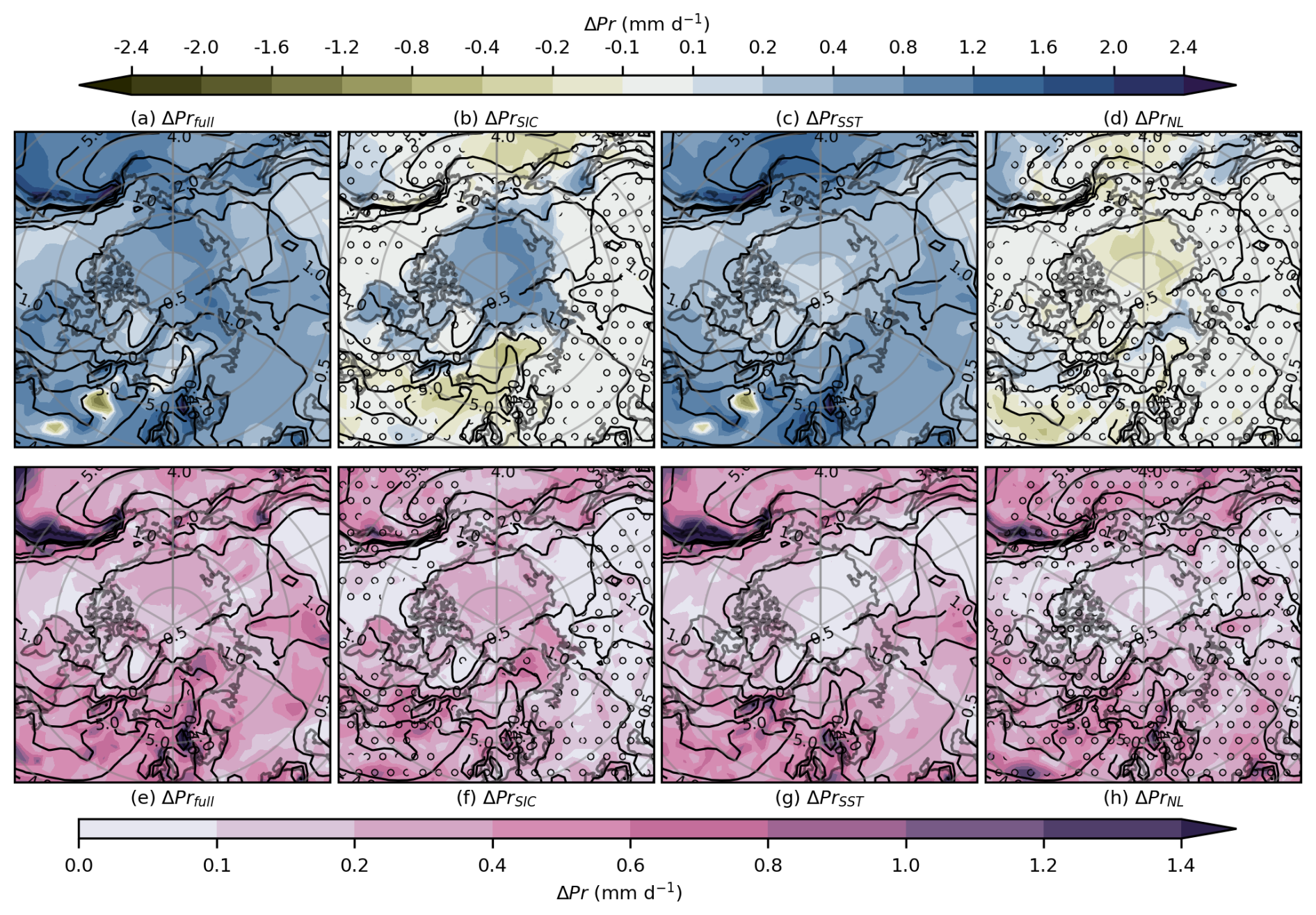
Figure 9 Difference in precipitation (Pr) in winter (DJF) between the SSP585 simulation and Baseline (ΔPr_full, a, e), between SIC_SSP585 and Baseline (ΔPr_SIC, b, f), between SST_SSP585 and Baseline (ΔPr_SST, c, g), and the non-linear (ΔPr_NL residual) contribution (d, h). The upper row (a–d) shows the multi-model mean, and the lower row (e–h) shows the maximum difference between models. Stippling indicates that all models do not agree on the direction of the change, and contours show the precipitation in the Baseline simulation.

3.4 Effect of surface fluxes

Changes in SST and sea ice cover affect the atmosphere mainly through surface fluxes of sensible and latent heat (Figs. S13 and S16). The increase in surface fluxes due to warmer SSTs occurs globally. In fact, the greatest increase takes place in the tropics and is driven by surface evaporation. This also leads to an increase in atmospheric heat and moisture content in polar regions through meridional transport, which makes the free troposphere in the polar regions warmer and more moist (Figs. S17 and S18). Furthermore, it increases the longwave emission towards the surface. In contrast, a decrease in sea ice cover mainly causes a local, near-surface climate response in the polar regions. The predominantly strongly stable stratification of the polar troposphere prevents the increased heat and moisture at the surface from reaching higher altitudes, and thus warming occurs only in the low troposphere of the polar regions (Fig. S17, ΔTSIC). Furthermore, moisture and heat fluxes over the sea equatorward from the original sea ice boundary tend to decrease (Figs. S11, S12, S14, and S15, ΔTSIC) because the air masses – which are advected equatorward from the areas that were originally covered by sea ice – have become warmer and more moist (not shown), which should decrease the temperature and humidity difference between the surface and the advected air mass. On a larger scale, the opposite changes in surface heat and moisture fluxes across the original sea boundary partly balance each other, which reduces the large-scale effect of decreasing sea ice cover.

Over areas where sea ice cover is reduced, our results also show that the sum of the individual effects of decreasing sea cover and increasing SSTs on 2 m temperatures is greater than the joint response (Figs. 4 and 7). In Baseline, surface heat fluxes are generally negative (downwards) or small over ice-covered areas, while they are positive (upwards) over oceans (not shown). When sea ice is removed, surface energy fluxes become positive over areas that used to be ice-covered. The fluxes are slightly higher (more positive) in the simulation where only sea ice cover is reduced (SIC_SSP585, Figs. S11, S12, S14, and S15) compared to the joint simulation (SSP585, Figs. S11, S12, S14, and S15). The reason is most likely that, during warm air intrusions (from lower latitudes) and cold air outbreaks (from snow- or ice-covered areas or sea ice), the air is slightly colder and drier in SIC_SSP585 than in SSP585, which enhances the fluxes over the ice-free ocean (where temperatures are set to the freezing point of seawater in both simulations). In the simulation where only SSTs are changed (SST_SSP585, Figs. S11, S12, S14, and S15), the surface fluxes become slightly more negative compared to the Baseline over areas covered by sea ice. This is probably due to the fact that the air is warmer and more moist during warm air intrusions from lower latitudes, which enhances the energy fluxes towards the surface.

3.5 Comparison between hemispheres

Spatial differences of the responses in meteorological variables between the poles are strongly linked to differences in the geographical environment. In addition, the overall stronger tropospheric warming in the Northern Hemisphere than in the Southern Hemisphere, due to an increased SST (Fig. S17), contributes to a stronger average increase in 2 m temperature in the Arctic compared to the Antarctic (Fig. 3a). One factor that contributes to the different responses of meteorological variables between the poles is the overall stronger warming in the Northern Hemisphere than in the Southern Hemisphere, due to increased SSTs (Fig. S17). However, the differences in the geographical environment also play an important role. In particular, the greater 2 m warming in the Arctic as compared to the Antarctic (Fig. 3a) is dominated by the strong near-surface warming due to sea ice loss in the Arctic. The warming is stronger in the Arctic because the original sea ice area is colder in the Arctic than in the Antarctic (Figs. 4 and 7). In addition, in the Arctic, the warming effect caused by a decrease in sea ice cover reaches further in over the continents than in the Antarctic, which may be a consequence of the high surface elevation of the Antarctic ice sheet preventing the direct advection of warm near-surface air over the continent. A similar but weaker feature is observed over Greenland where the change in 2 m temperature due to a sea ice decrease is weaker than in northern Canada or Siberia.

In both hemispheres, a decrease in sea ice cover causes increases in precipitation over the same area or the vicinity. Increases in surface latent heat fluxes (Figs. S14 and S15) and a subsequent weakening of the stable temperature stratification are probably behind this precipitation increase. However, the sea ice decrease has a notably stronger effect on precipitation in the northern polar region than in the southern. SST increases cause a widespread increase in precipitation in both polar regions, but the increase is slightly greater in the Arctic region than in the Antarctic region, most likely due to the overall stronger tropospheric warming and moistening in the Northern Hemisphere (Figs. S17 and S18).

In both hemispheres, the uncertainty associated with changes in MSLP is generally greater than the uncertainties associated with changes in 2 m temperature and precipitation. In the northern polar region, the decrease in sea ice cover has the greatest impact on MSLP, while warmer SSTs dominate the changes in MSLP at the south pole.

4 Discussion

We have used four AGCMs to study the effect of increasing SSTs and decreasing sea ice cover on polar climates. The experimental setup allows us to distinguish the relative contributions of sea ice decreases and SST increases to different climate variables in the polar regions as well as lower latitudes.

As sea ice is removed, the insulating layer between the sea water and atmosphere vanishes, which causes a significant increase in surface heat fluxes, leading to a strong local increase in 2 m temperature (Figs. 4 and 7). This effect dominates the change in 2 m temperatures during winter in the area and vicinity of the decreasing sea ice, in agreement with earlier studies (Screen et al., 2012; Screen and Blackport, 2019; Ye et al., 2024; Yu et al., 2024). In contrast, warmer SSTs have a greater effect on 2 m temperatures than a reduction in sea ice over the polar continents, which supports the results by Yu et al. (2024). In particular, in the inner Antarctic, the near-surface warming is strongly associated with the remote increase in SSTs. In contrast, the decrease in sea ice cover causes only small or even negative changes in 2 m temperature over the inner continent, most likely due to a weak advection of near-surface air from the ocean to the inner continent. Furthermore, at both poles, the SST increase causes mostly stronger 2 m temperature increases over the continents than over the ocean due to the overall tropospheric warming and increasing downwelling longwave radiation, which in turn is strongly driven by increased moisture in the troposphere and a higher tropospheric temperature, due to an increase in latent heat release. Overall, the effects of SST increase and sea ice decrease on 2 m temperature are linearly additive. However, the sum of the individual effects of decreasing sea cover and increasing SSTs on 2 m temperatures is sometimes greater than the joint response over areas where sea ice cover is reduced.

In agreement with earlier studies (e.g. Screen and Blackport, 2019; Streffing et al., 2021), we find that the uncertainty in the dynamical response (MSLP) is greater than in the thermodynamic response. However, the models in our study do agree on many features of the MSLP pattern changes, e.g. decreases in MSLP in the central Arctic and in the D'Urville Sea in the Antarctic. Previous studies (Yu et al., 2024; Ye et al., 2024; Smith et al., 2022; Chripko et al., 2021; Screen et al., 2018; Deser et al., 2010) have shown that reduced Arctic sea ice cover tends to increase the MSLP over the northern Atlantic, while it decreases over Siberia and the Aleutian region. These results generally agree with our SIC_SSP585 experiment, although some of the details in the pattern of the MSLP response differ. In particular, our multi-model mean response only shows an increase in MSLP over the Scandinavian side of the northern Atlantic, while the MSLP decreases over the Icelandic region and the western northern Atlantic. It is worth noting, however, that the models in our study do not agree on the direction of the MSLP response over the northern Atlantic, meaning that there is great uncertainty. Furthermore, in particular over the northern Atlantic, warmer SSTs generally produce a greater MSLP response than a decrease in sea ice cover in our simulations. Our multi-model mean results are produced from an ensemble of four models run for 40 years. Despite the many years of simulation, this may not be enough to capture the entire internal variability associated with dynamical variables such as MSLP, in particular in terms of their response to sea ice cover changes (Peings et al., 2021; Sun et al., 2022). Our ensemble is produced by four models, which should capture a larger part of the internal climate variability compared to an ensemble generated by only one model. However, our ensemble only represents two model families, meaning that the results are more dependent on each other than four completely independent models.

The precipitation response includes a thermodynamic response (increase in water vapour content), a local dynamic response (changes in e.g. convection), and a large-scale dynamic response (changes in e.g. storm tracks). Our simulations show that warmer SSTs generally increase precipitation in the polar regions, mainly due to the overall increase in atmospheric water vapour content (Fig. S18). Decreasing sea ice cover, on the other hand, mainly increases precipitation in areas where sea cover is reduced, indicating that enhanced local evaporation and convection during cold air outbreaks is the main cause of precipitation changes. In general, this result is in agreement with previous studies (Yu et al., 2023, 2024) and can be linked to the high warming scenario (SSP5-8.5) where thermodynamic and local effects are expected to dominate over large-scale dynamic effects in terms of changes in precipitation (Yu et al., 2023, 2024).

5 Conclusions and perspectives

We have used four AGCMs to examine the climate response in the polar regions and lower latitudes to prescribed future global changes in SST and sea ice cover, with a focus on wintertime 2 m temperatures, MSLP, and surface precipitation at high latitudes. Generally, the models agree on the response in 2 m temperature and surface precipitation, in particular in terms of the spatial distribution and the relative impact of warming SSTs and decreasing sea ice cover. The models agree less well on the magnitude and spatial distribution of the MSLP response; i.e. the uncertainties associated with the atmospheric circulation response are greater than the uncertainties associated with the thermodynamic response. The models agree on an increase in MSLP in the central Arctic and Bering Strait as well as in the D'Urville Sea in the Antarctic but disagree on the changes over northern Europe and the northern Atlantic.

Changing sea ice cover and SSTs cause about the same average warming poleward of 60° N/S in winter, whereas warmer SSTs increase precipitation more strongly than decreasing sea ice cover. This result applies to both poles and implies that a substantial part of the polar near-surface warming and precipitation increase is a response to remote SST forcing. Furthermore, increasing SSTs cause an overall greater tropospheric warming and moistening of the Northern Hemisphere, which contributes to stronger increases in precipitation and 2 m temperature in the Arctic than in the Antarctic. The MSLP response to changing SSTs tends to be of approximately similar magnitude (Arctic) or greater (Antarctic) than the response to changing sea ice cover – and the responses sometimes counteract each other. Warmer SSTs also have a widespread impact on 2 m temperatures and precipitation, while a decrease in sea ice cover mainly causes a localized response; i.e. the warming and increased precipitation tend to occur in the areas (or in the vicinity of the areas) where the sea ice disappears. The reason for this localized response is most likely the strong temperature stratification in the polar regions in winter, which prevents the increased surface heat fluxes from affecting higher levels of the atmosphere. Thus, a decrease in sea ice cover produces a weak effect on the thermodynamic variables outside the areas of sea ice retreat. SST changes dominate the polar 2 m temperature and precipitation responses outside the areas of sea ice retreat, including the Antarctic continent.

The models predict that the change in 2 m temperature and precipitation at both poles is generally linear; i.e. the modelled response to simultaneous changes in SSTs and sea ice is approximately equal to the sum of the individual changes. The main exceptions are the areas within and in the vicinity of the zone of sea ice retreat. Over these areas, the sum of the individual responses in 2 m temperature and precipitation to decreasing sea ice cover and increasing SSTs is greater than the joint effect. This result suggests that some of the polar warming that is caused by warmer SSTs outside the polar regions (and subsequent increased large-scale heat and moisture transport) weakens the contribution of turbulent surface fluxes to polar warming; i.e. the remote response weakens the local response.

At both poles, our results show that the greatest uncertainty in the climate response to decreases in sea ice cover and warmer SSTs is associated with atmospheric circulation, as the most significant differences between the models was found for MSLP. Note that these discrepancies occurred even though the models were constrained by the same oceanic boundary conditions. The circulation response to decreasing sea ice cover was sometimes enhanced but sometimes also counteracted by the response to warmer SSTs. This finding is particularly important to consider when drawing conclusions about changes in mid-latitude circulation to changing sea ice cover using either observations or model simulations where the two effects (from decreasing sea ice and changing SSTs) cannot easily be separated. Furthermore, to decrease the uncertainty and improve our confidence in climate predictions, it is important to disentangle the causes behind the differences in the circulation responses between the models. The model setup and output presented here are unique in this respect and can be used to explore the underlying physical processes.