South Asia anthropogenic ammonia emission inversion through assimilating IASI observations

Ammonia has attracted significant attention due to its pivotal role in the ecosystem and its contribution to the formation of secondary aerosols. Developing an accurate ammonia emission inventory is crucial for simulating atmospheric ammonia levels and quantifying its impacts. However, current inventories are typically constructed via the bottom-up approach and are associated with substantial uncertainties. To address this issue, assimilating observations from satellite instruments for top-down emission inversion has emerged as an effective strategy for optimizing emission inventories. Despite the severity of ammonia pollution in South Asia, research in this context remains very limited. This study aims to estimate ammonia emissions in this region by integrating the prior emission inventory from the Community Emissions Data System (CEDS) and the columned ammonia concentration retrievals from the Infrared Atmospheric Sounder Interferometer (IASI). We employ a newly developed four-dimensional ensemble variational (4DEnVar)-based emission inversion system to conduct the calculations, resulting in monthly ammonia emissions for 2019 at a resolution of 0.5° × 0.625°. The annual total estimate for the posterior emission inventory is 12.61 Tg, compared to the prior inventory's 13.32 Tg. Our simulations, driven by the posterior emission inventory, demonstrate superior performance compared to those driven by the prior emission inventory. This performance is validated through comparisons against the IASI observations, the independent column concentration measurements from the advanced satellite instrument Cross-track Infrared Sounder (CrIS), and the ground concentration observations of ammonia and PM_2.5. Additionally, the spatial and temporal characteristics of ammonia emissions in South Asia based on the posterior inventory are analyzed. Notably, emissions there exhibit a “double-peak” seasonal profile, with the maximum in July and the secondary peak in May. This observation differs from the “double-peak” trend suggested by the CEDS prior inventory, which identifies the maximum column concentration in May and a second peak in September. The differences may be attributed to a more accurate representation of regional agricultural practices, such as the timing of fertilizer application and meteorological influences like precipitation and temperature.

1 Introduction

Ammonia (NH₃), an alkaline compound, has the capacity to react with acidic gases present in the atmosphere, thereby contributing to the formation of secondary aerosols, notably ammonium sulfate and ammonium nitrate (Jimenez et al., 2009). The genesis of fine atmospheric particulate matter poses significant threats to human health (Mukherjee and Agrawal, 2017). Further, ammonia gas, along with its reaction products, plays a pivotal role in soil acidification and the eutrophication of water bodies through both dry and wet deposition (Krupa, 2003), thereby affecting the balance of ecosystems (Asman et al., 1998) and climate change (Ma et al., 2022; Gong et al., 2024). With an enormous livestock population and extensive use of nitrogen fertilizers, South Asia has experienced the highest level of atmospheric NH₃ globally (Pawar et al., 2021; Luo et al., 2022). Specifically, the annual average ammonia concentration across India is approximately 1.8–5.6 × 10¹⁶ mol cm⁻², while in the Indo-Gangetic Plain (IGP) of India, the concentration is double that of other regions, reaching a peak of 11.5 × 10¹⁶ mol cm⁻² during the high season in July (Kuttippurath et al., 2020).

Over the past decade, scientists have predominantly employed the “bottom-up” approach to estimate NH₃ emissions. When combined with chemical transport models, atmospheric NH₃ dynamics can be simulated, enabling the quantification of environmental impacts. Substantial efforts have been made to quantify the spatiotemporal distribution of NH₃ sources and develop global/regional emission inventories, such as the global NH₃ emission inventory (Bouwman et al., 1997), the anthropogenic emission inventory that includes NH₃ estimates (e.g., Community Emissions Data System, or CEDS) (Hoesly et al., 2018a), and regional NH₃ inventories focusing on South Asia (Yan et al., 2003; Yamaji et al., 2004; Liu et al., 2022). However, these bottom-up estimates of NH₃ emissions are generally considered as uncertain (Xu et al., 2019), particularly when compared with emissions of other pollutants primarily originating from fossil fuel combustion, such as NO₂. One challenge is that the intensity of agricultural NH₃ emissions (i.e., emission factors), whether from livestock or fertilizer, depends heavily on management and farming practices, but this information is often not readily available (Zhang et al., 2017). As a result, atmospheric chemistry transport models driven by these emission estimates inevitably struggle to reproduce atmospheric NH₃ concentrations. Consequently, these discrepancies hinder our comprehensive understanding of the environmental implications of NH₃ emissions.

The rapid advancement of satellite remote sensing technology has resulted in an expanding array of valuable NH₃ products, such as those from the first satellite NH₃ observations using the Tropospheric Emission Spectrometer (TES) (Beer et al., 2008), as well as higher-resolution retrievals from the Infrared Atmospheric Sounding Interferometer (IASI) (Pawar et al., 2021) and the Cross-track Infrared Sounder (CrIS) (Beale et al., 2022; Kharol et al., 2022). While these remote sensing measurements play a pivotal role in characterizing atmospheric NH₃ loading, limitations still remain. These primarily arise from the fact that satellite observations can only measure column-integrated NH₃ concentrations, which do not directly reflect emission intensity or the three-dimensional concentration field. In addition to these satellite-based data, very limited ground-based observations are publicly available over South Asia, and those that do exist are constrained by their inadequate representation of atmospheric NH₃ features (Pawar et al., 2021).

In the field of atmospheric pollutant modeling, an alternative method for calculating emission flux is the “top-down” approach, which is achieved through data assimilation. Over the past decade, emission inversion has gained widespread attention globally and has been applied in various contexts, including the estimation of volatile organic compounds (VOCs) (Bauwens et al., 2016; Choi et al., 2022), sulfur dioxide (SO₂) (Qu et al., 2019; Li et al., 2021), methane (CH₄) (Wecht et al., 2014; Fujita et al., 2020), and atmospheric NH₃ emissions. For example, Kong et al. (2019) calculated the 2016 NH₃ emission inventory in China by assimilating ground-based NH₃ concentration observations from several dozen ground stations. Similarly, Chen et al. (2021) optimized the prior NH₃ emission estimates from the United States' 2011 National Emissions Inventory (2011 NEI) by assimilating NH₃ column concentrations from IASI instruments across the United States. Recently, we developed a four-dimensional variational assimilation-based NH₃ emission inversion system, which has been successfully tested for NH₃ emission inversion by assimilating IASI products over China.

However, there is a paucity of studies focusing on assimilation-based NH₃ emission inversion specific to South Asia, which has some of the highest NH₃ loading hotspots compared to other continents. In this study, we aim to explore the spatial and temporal features of NH₃ emissions over South Asia. The NH₃ emission inventory will be calculated using our newly developed emission inversion system (Jin et al., 2023) by assimilating NH₃ retrievals from the IASI instruments on board the MetOp-A (operational from 2008 to 2018), MetOp-B (operational since 2012), and MetOp-C (operational since 2018) satellites (MetOp stands for Meteorological Operational). Instead of directly assimilating IASI measurements as previous studies have done, we incorporate the averaging kernel information from the latest version of the IASI product. This approach allows us to update the column concentration observations before assimilation. By doing so, we ensure a fairer comparison between the simulated and observed columnar NH₃ concentrations, a point that has been emphasized in several studies (Eskes and Boersma, 2003; von Clarmann and Glatthor, 2019) but never implemented in the IASI-based emission inversion. We aim to provide a more accurate estimation of anthropogenic NH₃ emission inventories and to explore their spatial and temporal characteristics across South Asia. Additionally, this work serves as a model for effectively calculating atmospheric pollution emissions in regions that have been less studied in the past. The study focuses on anthropogenic NH₃ emissions but also contributes to a broader understanding of atmospheric pollution in under-researched regions.

The remaining sections of this paper are organized as follows. Section 2 describes the measurements assimilated in the NH₃ emission inversion, as well as those used for independent validation. The assimilation methodology for the emission inversion, along with the choice of the prior emission inventory and the chemical transport model, is also outlined. Section 3 presents the validation results of the emission inversion and highlights the key features of NH₃ emissions over South Asia.

2 Data and method

2.1 IASI satellite measurements

IASI (Infrared Atmospheric Sounding Interferometer) is a Fourier transform spectrometer that operates in the thermal infrared spectral range. It is on board the MetOp-A, MetOp-B, and MetOp-C satellites, a series of European polar-orbiting meteorological satellites managed by the European Space Agency (ESA) and the European Organization for the Exploitation of Meteorological Satellites (EUMETSAT). The MetOp-A satellite, equipped with IASI, was launched in 2008, followed by MetOp-B and MetOp-C in 2012 and 2018, respectively. The IASI instruments operate at an altitude of 817 km in a sun-synchronous orbit with an inclination of 98.7°. Each instrument conducts measurements over a ground swath width of 2200 km, with 30 fields of view (15 on each side of the nadir). Each field of view consists of four pixels, each with a nadir diameter of 12 km. This observational strategy enables each IASI instrument to make two passes over every point on Earth daily, around 09:30 and 21:30 local time (Bouillon et al., 2020).

The assimilated observations for estimating the NH₃ emissions were the monthly IASI column concentration means over the 0.5° × 0.625° GEOS-Chem grid cell. These values were derived from the latest ANNI-NH₃-v4R-ERA5 product. Despite improvements in NH₃ column retrievals from satellite observations, there remains substantial variability in measurement uncertainty, ranging from 5 % to over 1000 % (Van Damme et al., 2014; Whitburn et al., 2016; Van Damme et al., 2017). Data selection was performed by excluding nighttime observations, irrational values (<0), and using only data with a cloud fraction <0.1 (Van Damme et al., 2018) and skin temperature >263 K (Van Damme et al., 2014) during the calculation of the monthly mean. While negative values are not necessarily incorrect, they are considered unrealistic in the context of NH₃ concentrations. To improve the quality of the monthly average, we removed those negative values. Additionally, we re-compared the cases of excluding negative NH₃ total column values and retaining them. As shown in Fig. S1 in the Supplement, the positive bias on the final concentrations within our study region is minimal. It is also important to note that we used daily observations from three satellites, each with a pixel resolution of approximately 12 km × 12 km, which provided us with sufficient observations to calculate the monthly average. We applied a selection criterion, using only grid averages that contain a minimum of 80 observations. This approach ensures that the grid-averaged values are statistically representative and that the monthly mean is of high quality. Notably, the time coverage of the available version 4 IASI product used was limited: MetOp-A provided data for the entire year of 2019, MetOp-B provided data from January to July 2019, and MetOp-C did not have data for 2019. Therefore, only the data from MetOp-A and MetOp-B within the 2019 time frame were used in this study. The use of both MetOp-A and MetOp-B data for 2019 ensures data continuity and enhances the reliability of the measurements. While a single satellite could provide sufficient data, using both platforms could improve temporal and spatial coverage, resulting in more accurate and robust results. To ensure robustness, we also made a brief comparison of the NH₃ column concentrations obtained from both MetOp-A and MetOp-B satellites, as shown in Fig. S2. Despite some small differences, the data from both satellites are generally consistent in terms of spatial patterns and concentration levels. Additionally, the data from the two satellites can complement each other, indicating good reliability of the results across both platforms. To further improve the data quality and ensure consistency, we performed monthly and grid averaging of the observations. This approach not only allows for a fair comparison between the observed and modeled NH₃ concentrations but also reduces the computational cost of the assimilation process. Using individual observations without averaging would result in an excessively large observational vector, which would significantly increase the computational burden. For example, without averaging, the size of the observational vector could reach 1 000 000, while with monthly and grid averaging, it is reduced to a manageable size of around 1000. This reduction in size helps to optimize the data assimilation process while maintaining the integrity of the emission estimates.

Compared to the previous version, one highlight of the latest version 4 product is that it includes averaging kernel information. The benefit of using the averaging kernel is that it can consider the vertical distribution characteristics of satellite observations, helping to correct the satellite retrieval results and making them more representative of the true distribution of the target gas or variable in the atmosphere (Rodgers, 2000). The impact of averaging kernels (AVKs) is supposed to be considered in the data processing. The sensitivity of IASI NH₃ observations varies with altitude, and AVKs enable the adjustment of simulated or observed NH₃ concentrations to align with the vertical distribution detected by IASI. This adjustment is particularly important for data comparison and validation against the model simulations (Clarisse et al., 2023). The formula for calculating the column concentration, after accounting for the averaging kernels, in this paper follows:

$$\begin{array}{}\text{(1)}& {\widehat{X}}^{\mathrm{m}}={\displaystyle \frac{{\widehat{X}}^{\mathrm{a}}-B}{{\sum }_z{A}_z^{\mathrm{a}}{m}_z}}+B.\end{array}$$

Here, ${\widehat{X}}^{\mathrm{m}}$ represents the IASI column concentration retrieved with the model profile. ${\widehat{X}}^{\mathrm{a}}$ denotes the initial IASI column concentration, with the background concentration B. The $A_z^{\mathrm{a}}$ values are the AVK for each vertical layer, with the model profile m_z. More detailed information and the corresponding equations are provided in the Supplement, Eqs. (S8) and (S9).

The uncertainty assigned to the IASI measurements is also essential. When calculating the uncertainty of gridded monthly average NH₃ measurements, both instrumental errors σ^instrumental and the representation error σ^{representation} are considered. The gridded average uncertainty derived directly from IASI products was designated as the instrumental error σ^instrumental, while the standard deviation of the observed samples for the gridded average was characterized as the representation error σ^{representation}. The total uncertainty σ^integrated for weighting the potential spread of the assimilated IASI NH₃ measurements is finally expressed as:

$$\begin{array}{}\text{(2)}& {\mathit{\sigma }}^{\text{integrated}}={\left\{{\left({\mathit{\sigma }}^{\text{instrument}}\right)}^{\mathrm{2}}+{\left({\mathit{\sigma }}^{\text{representing}}\right)}^{\mathrm{2}}\right\}}^{\mathrm{0.5}}.\end{array}$$

Four snapshots of the assimilated monthly IASI NH₃ column concentration observations and their uncertainty in January, April, July, and November can be found in Figs. 1a and S3. These four scenarios are selected to highlight the typical seasonal profile of the NH₃ loading over South Asia.

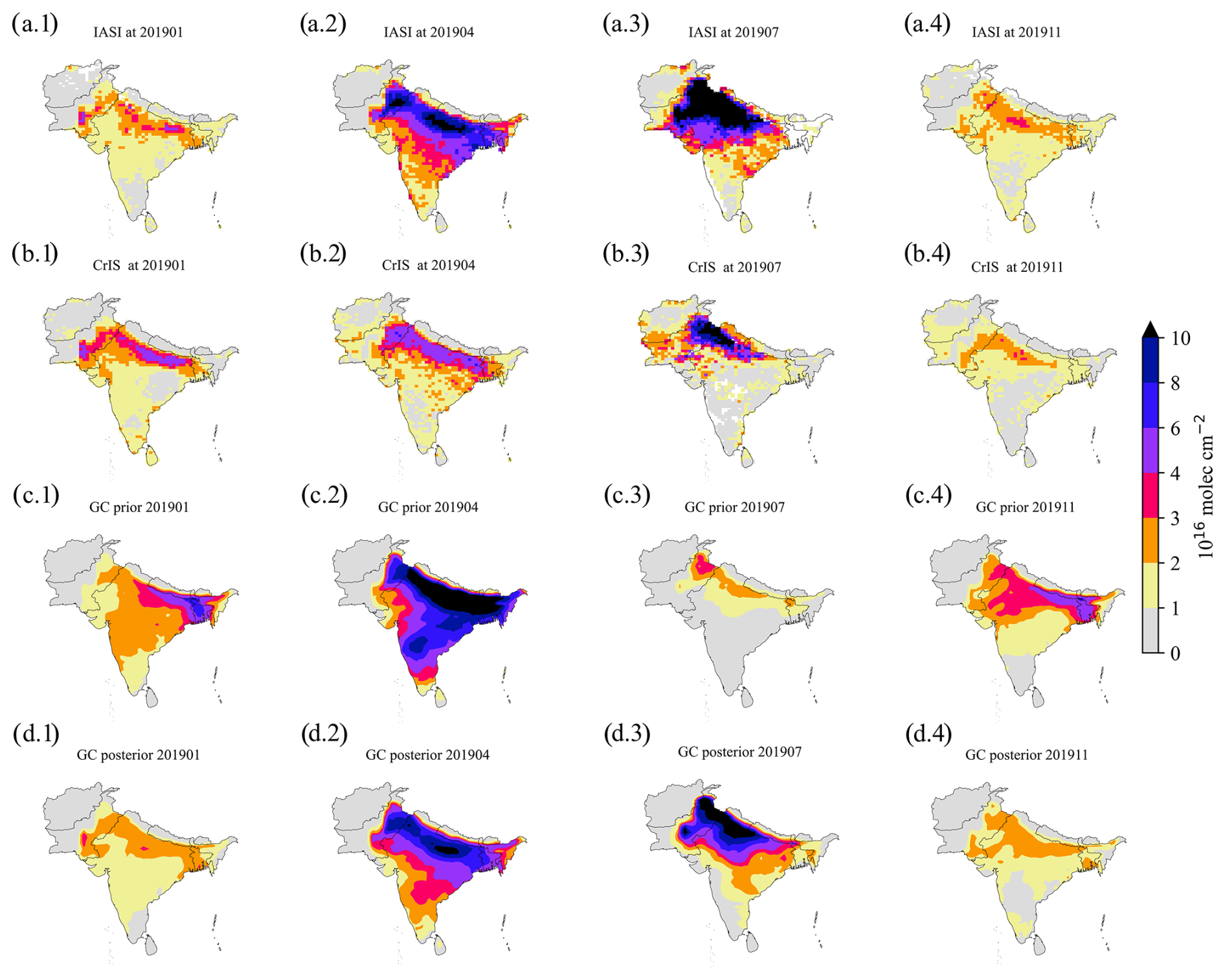
Figure 1 Spatial distribution of the total column NH₃ concentration from the IASI (a) or CrIS (b) instruments and from the GEOS-Chem simulation using either the prior (c) or the posterior (d) NH₃ emission flex for January (a.1–d.1), April (a.2–d.2), July (a.3–d.3), and November 2019 (a.4–d.4).

2.2 Independent observations for validation

The Cross-track Infrared Sounder (CrIS) NH₃ column concentration and ground-based observations of NH₃ and PM_2.5 from the Central Pollution Control Board (CPCB) of India were also collected to validate our assimilation results.

The CrIS instrument was launched in 2011 on the Suomi National Polar-Orbiting Partnership (SNPP) satellite and in 2017 on the NOAA-20 satellite. The retrieval products from SNPP began in 2011 and ended in May 2021, with a data gap from April to August 2019. The NH₃ retrieval products from NOAA-20 started in March 2019. Therefore, we used retrieval products from both SNPP and NOAA-20 as independent observations for 2019. We utilized the Level 2 CrIS product from the CFPR 1.6.4 version. Specifically, only the CrIS observations during daytime, under cloud-free conditions, and with a quality flag ≥3 were selected. These original data were subsequently interpolated to achieve a spatial resolution of 0.5° × 0.625°, which is consistent with our NH₃ simulation. Similarly, we also considered the impact of the averaging kernels (AVKs) and applied the AVKs to the satellite profile data. We converted the logarithmic averaging kernels into linearized averaging kernels based on the method proposed by Cao et al. (2022).

Ground observations of NH₃ in South Asia are mainly provided by the Central Pollution Control Board (CPCB, https://cpcb.nic.in/, last access: 21 October 2024), which is the official portal of the Government of India. NH₃ is measured by the chemiluminescence method as NO_x following the oxidation of NH₃ to NO_x. In that approach, NH₃ is determined from the difference between the NO_x concentration with and without the inclusion of NH₃ oxidation (Pawar et al., 2021). The ground-level NH₃ concentration data from CPCB were successfully collected. There were NH₃ surface concentration observations from 33 stations available in 2019; the distribution of these stations is shown in Fig. 2.

PM_2.5 observations from CPCB were also used in the assimilation validation. The PM_2.5 observations were selected before they were used, which follows (Spandana et al., 2021): First, select the hourly PM_2.5 data greater than PM₁₀. Then, filter out the hourly PM_2.5 data that fall outside the range of day_mean − 3 × standard deviation and day_mean + 3 × standard deviation. Additionally, ensure that each day contains at least 20 h of data. Finally, process the data into monthly averages for subsequent validation. The distribution of the ground stations where the PM_2.5 values were used in this paper can be found in Fig. 2, and detailed information about the stations is provided in Tables S1–S3 in the Supplement.

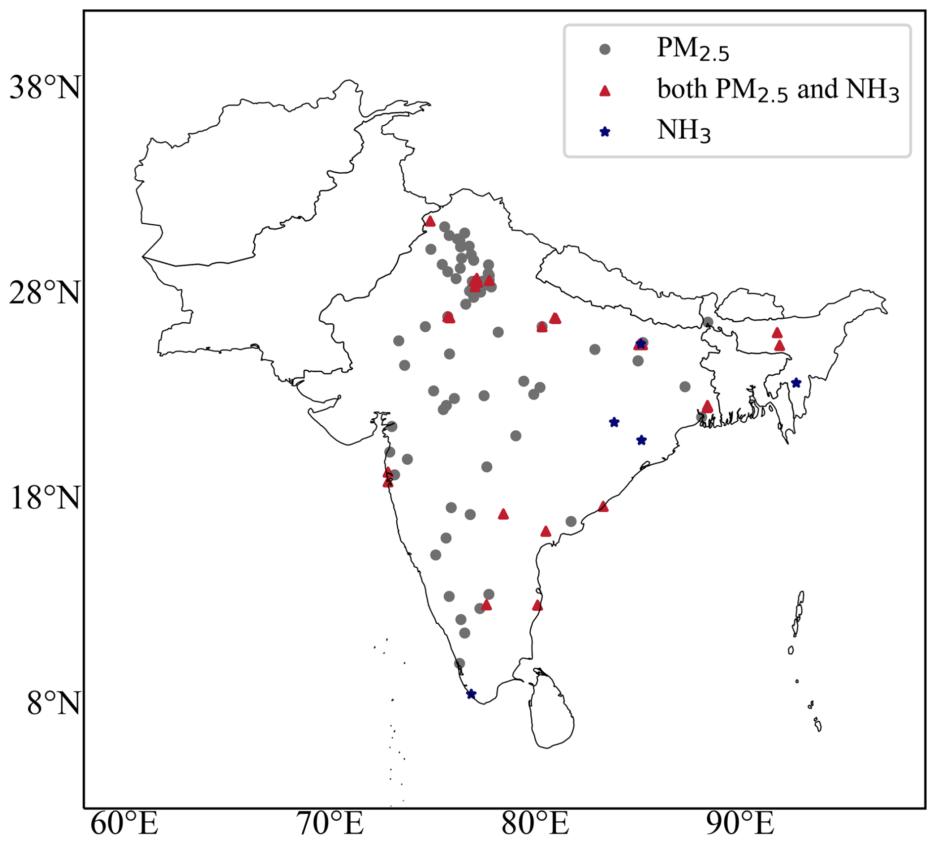
Figure 2 The GEOS-Chem model simulation domain, with dots indicating the locations of ground observation stations from the Central Pollution Control Board (CPCB), India. The three different-colored dots represent stations with only PM_2.5 observations, stations with both PM_2.5 and NH₃ observations, and stations with only NH₃ observations.

2.3 Emission inversion system

This study employs the four-dimensional ensemble variational (4DEnVar) data assimilation-based NH₃ emission inversion system that was developed by Jin et al. (2023). The general idea of assimilation-based emission inversion is to find the most likely estimate, which in this case is the monthly NH₃ emission field, given the prior NH₃ emissions and the observations. The calculation is conducted through minimizing the cost function 𝒥:

$$\begin{array}{}\text{(3)}& \begin{array}{rl}\mathcal{J}\left(\mathit{f}\right)& ={\displaystyle \frac{\mathrm{1}}{\mathrm{2}}}{\left(\mathit{f}-{\mathit{f}}_b\right)}^{\mathrm{T}}{\mathbf{B}}^{-\mathrm{1}}\left(\mathit{f}-{\mathit{f}}_b\right)\\ & +{\displaystyle \frac{\mathrm{1}}{\mathrm{2}}}\mathit{\{}\mathit{y}-\mathbf{H}\mathcal{M}(\mathit{f}\left){\mathit{\}}}^{\mathrm{T}}{\mathbf{O}}^{-\mathrm{1}}\mathit{\right\{}\mathit{y}-\mathbf{H}\mathcal{M}\left(\mathit{f}\right)\mathit{\}}\end{array}.\end{array}$$

Here, f denotes the vector of the NH₃ estimated emission field, with its units typically expressed in kg m⁻² s⁻¹. Additionally, f_b denotes the prior monthly NH₃ emission vector from CEDS, as will be described in Sect. 2.4. B represents the background error covariance matrix associated with the prior emission estimate. Here, we assume that the uncertainty in the NH₃ emission can be compensated by a spatially varying tuning factor α. The α values are defined to be random variables with a mean of 1.0 and a standard deviation σ=0.2. In addition, a correlation matrix C is introduced for quantifying the spatial correlation between two α values in the grid i and j as:

$$\begin{array}{}\text{(4)}& \mathbf{C}(i,j)=e^{-(d_{i,j}/l{)}^{\mathrm{2}}/\mathrm{2}},\end{array}$$

where d_i,j represents the distance between two grid cells i and j. l here denotes the correlation length scale, which controls the spatial degrees of freedom of the α values. An empirical parameter l=300 km, which is used in the NH₃ emission inversion in China (Jin et al., 2023), is also used in this study. With the spatial correlation matrix and the emission uncertainty, the background error covariance matrix could then be constructed as:

$$\begin{array}{}\text{(5)}& \mathbf{B}(i,j)={\mathit{\sigma }}^{\mathrm{2}}\cdot {\mathit{f}}_b\left(i\right)\cdot {\mathit{f}}_b\left(j\right)\cdot \mathbf{C}(i,j).\end{array}$$

ℳ here represents the GEOS-Chem model (as will be illustrated in Sect. 2.4) driven by the emission f. H is the observational operator that transfers the simulated NH₃ 3D concentration result into the observational space. y represents the monthly IASI NH₃ column concentration observations, while O is the observation error covariance matrix. Here, we assume the IASI observation representation errors are independent from each other. O therefore is a diagonal matrix filled with the square of the integrated uncertainty, as described in Sect. 2.1. Meanwhile, a minimum measurement error is used to prevent the posterior from being too close to low-value observations, thereby avoiding model divergence:

$$\begin{array}{}\text{(6)}& {\mathbf{O}}_{i,i}=min{\left(\mathrm{1.0}\times {\mathrm{10}}^{\mathrm{16}}{\text{molec\hspace{0.17em}cm}}^{-\mathrm{2}},{\mathit{\sigma }}^{\text{integrated}}\right)}^{\mathrm{2}}.\end{array}$$

More information about how we minimize the cost function Eq. (3) can be found in Jin et al. (2023).

2.4 GEOS-Chem model and emission inventory

GEOS-Chem, a three-dimensional (3-D) global tropospheric chemistry model, is driven by assimilated meteorological data obtained from the Goddard Earth Observing System (GEOS) at the NASA Data Assimilation Office (DAO) (Bey et al., 2001). GEOS-Chem incorporates a fully integrated chemistry system involving aerosol, ozone, NO_x, and hydrocarbons, as described by Park et al. (2004). The wet deposition scheme is explained by Liu et al. (2001) for water-soluble aerosols and by Amos et al. (2012) for gaseous components. Dry deposition is modeled using the resistance-in-series scheme proposed by Wesely and Lesht (1989), as applied by Wang and Jacob (1998). Size-specific aerosol dry deposition follows the approach outlined by Emerson et al. (2020).

Table 1 The use of observations and simulations.

A nested grid simulation within the GEOS-Chem model v13.4.1 is conducted to simulate the atmospheric environment over South Asia. The nested domain (60–98° E, 4–40° N), shown in Fig. 2, has a horizontal resolution of 0.5° latitude by 0.625° longitude, accompanied by 47 vertical layers. The model is driven by meteorological fields from the Modern-Era Retrospective analysis for Research and Applications, Version 2 (MERRA-2) reanalysis dataset provided by the Global Modeling and Assimilation Office (GMAO) at NASA. The model employs a 3 month spin-up period to minimize the influence of the initial conditions. Lateral boundary conditions for the nested domain are updated every 3 h using output from the global GEOS-Chem simulation at 2° × 2.5° resolution. Chemical initial conditions are also obtained from the global simulation to ensure consistency.

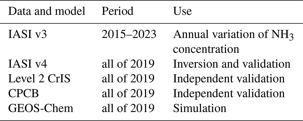
The NH₃ emissions inventory employed to drive GEOS-Chem originated from the Community Emissions Data System (CEDS, https://doi.org/10.25584/PNNLDH/1854347, Hoesly et al., 2018b) inventory, which has been widely used for modeling the South Asia atmospheric pollutants, e.g., VOCs (Chaliyakunnel et al., 2019) and PM_2.5 pollution (Guttikunda and Nishadh, 2022; Xue et al., 2021). The CEDS inventory includes various sources encompassing agricultural, energy production, industrial, residential, and commercial activities, ships, solvent use, surface transportation, and waste processing (McDuffie et al., 2020). The bulk of NH₃ emissions originate from agricultural practices. Specifically, these emissions stem predominantly from farmlands, including crops such as wheat, maize, and rice, as well as manure from livestock, including cattle, chicken, goats, and pigs (Liu et al., 2022). The CEDS emission estimates were coarse-grained into the model resolution 0.5° × 0.625° before being utilized to drive the GEOS-Chem simulations. Examples of the CEDS emission over South Asia are presented in Fig. 3, which plots the total NH₃ emission fluxes for January, April, July, and November of the year 2019. Additionally, the model's biogenic emissions are based on the MEGAN2.1 (Model of Emissions of Gases and Aerosols from Nature) inventory (Guenther et al., 2012), while the biomass burning sources driving the model are based on the GFEDv4 (Version 4 of the Global Fire Emissions Database) inventory (Giglio et al., 2013). The use of IASI and CrIS observations, along with GEOS-Chem simulations, is outlined in Table 1.

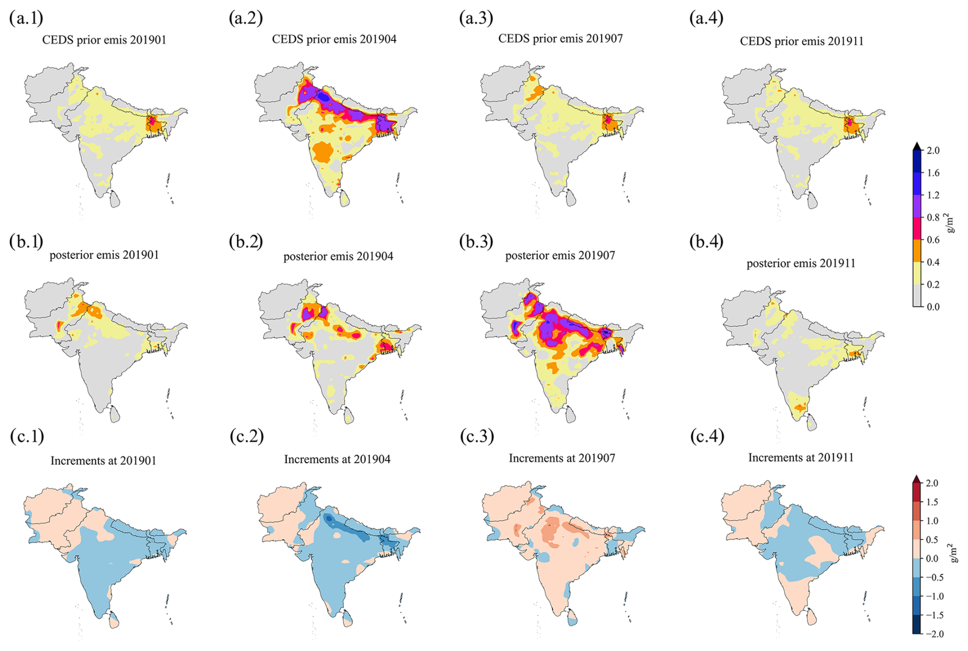
Figure 3 Spatial distribution of the prior (a), the posterior (b), and the posterior minus prior increments (c) monthly NH₃ emission in January (a.1–c.1), April (a.2–c.2), July (a.3–c.3), and November 2019 (a.4–c.4).

3 Results and discussion

With the assimilation system described above, the monthly anthropogenic NH₃ emission inversion for 2019 over South Asia is conducted. The spatial distribution of the prior and posterior results is presented in Sect. 3.1.1. The long-term varying trend of South Asia NH₃ emission is illustrated in Sect. 3.1.2, followed by an analysis and discussion of its spatial distribution and seasonal profile based on the inversion results in Sect. 3.2. Then, the posterior result is evaluated in Sect. 3.3.

3.1 Observed NH₃ concentrations

We first present the spatial distribution of NH₃ column concentrations from satellite observations and model results driven by either the prior or posterior inventories. Then, we examine their seasonal variation in 2019 and the long-term trends from 2015 to 2023.

3.1.1 Spatial NH₃ total column concentration

The prior and posterior snapshots of NH₃ column concentration simulations for four months (January, April, July, and November) are presented in Fig. 1c–d, alongside the IASI measurements, shown in panel (a). These months were selected as typical examples representing four different seasons. The column concentration distributions for the remaining months from the model and satellite observations can be found in Figs. S4 and S5, respectively. While the prior simulation generally captured the distribution of NH₃, with hot spots in North India, Pakistan, and Bengal – consistent with the IASI retrievals – it failed to capture the correct seasonal profile. According to the IASI measurements, NH₃ concentrations peak in July, a pattern clearly visible in the monthly variation of the IASI-observed NH₃ column concentrations from 2015 to 2023, as will be discussed in Sect. 3.1.2. However, the prior model incorrectly indicated that the highest NH₃ loading occurred in the spring and autumn seasons. As a result, NH₃ loading was severely overestimated in winter and spring (particularly in May) but significantly underestimated in summer.

Note that there are still some discrepancies in the posterior simulation vs. IASI column measurements. In particular, as shown in panel (a.3) vs. (d.3) of Fig. 1, the posterior simulation did not fully reproduce the extremely high NH₃ loading observed by IASI in July (with column-integrated concentrations exceeding 10 × 10¹⁶ molec. cm⁻²). This outcome occurs because the goal of the assimilation is to achieve the best fit between the posterior, observed, and prior emissions rather than just fitting the observations alone. The extremely high NH₃ concentrations are less likely given the relatively low prior NH₃ emissions and the background error covariance matrix described in Sect. 2.3. Additionally, the 4DEnVar assimilation algorithm inherently accounts for potential model variations through ensemble simulations. However, the response of GEOS-Chem NH₃ simulations to emission variations is nonlinear, making it difficult to accurately resolve these discrepancies through the 4DEnVar data assimilation algorithm without implementing outer-loop optimization strategies. Additionally, the spatial distribution of the NH₃ column concentrations observed by CrIS, as shown in panel (b) of Fig. 1, demonstrate good consistency with both the IASI observations and the posterior simulation results presented in Fig. 1.

3.1.2 Seasonal and annual variation of NH₃ concentration

We examined the monthly average of the total NH₃ column concentrations simulated by the model over the South Asia region, along with IASI and CrIS observations, in Fig. 4a. The prior model results demonstrate significant seasonal variability in NH₃ column concentrations, characterized by peaks in May and September and comparatively low levels during the summer months. This variability has been corrected through assimilating the IASI measurements in this study. Conversely, the posterior results reveal a distinct temporal pattern, featuring a pronounced peak in May and a negligible peak in July. The high value in May is attributed to the huge amount of biomass burning in South Asia during the spring in Fig. S6c. We identified the planting and harvesting times of crops in the South Asia region based on information from the U.S. Department of Agriculture (USDA, https://ipad.fas.usda.gov/rssiws/al/crop_calendar/sasia.aspx, last access: 3 March 2025), as presented in Table 2. The heavy use of fertilizers in agricultural activities has resulted in the highest emission throughout the year, as will be illustrated in Fig. 4b in Sect. 3.2. This lead to the second NH₃ concentration peak in July. The reasons for higher emissions in July but lower concentration levels compared to May could be attributed to meteorological factors. The monsoon season in South Asia results in increased wet deposition, and, notably, 2019 experienced the most intense monsoon since 1994 (Bhargavi et al., 2024). As shown in Fig. S6a and b, the precipitation and temperature in July are the highest of the year. High temperature could increase ammonia volatilization, leading to higher concentrations, while high precipitation increases the wet deposition of ammonia. However, the impact of temperature on concentration is secondary compared to the dramatic variations in precipitation. These combined factors result in July having a smaller concentration peak compared to May, despite July being another peak month. Additionally, CrIS exhibits minor peaks in May and July, consistent with our posterior results.

Table 2 Crop calendars for selected Kharif crops in Bhutan, India, Nepal, and Pakistan from USDA.

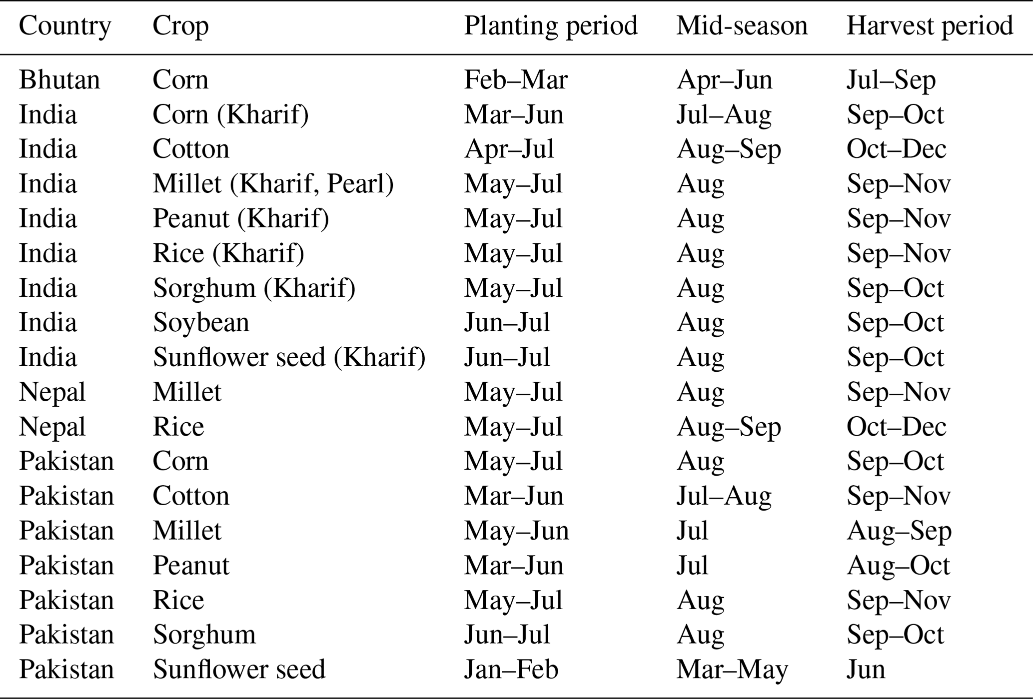
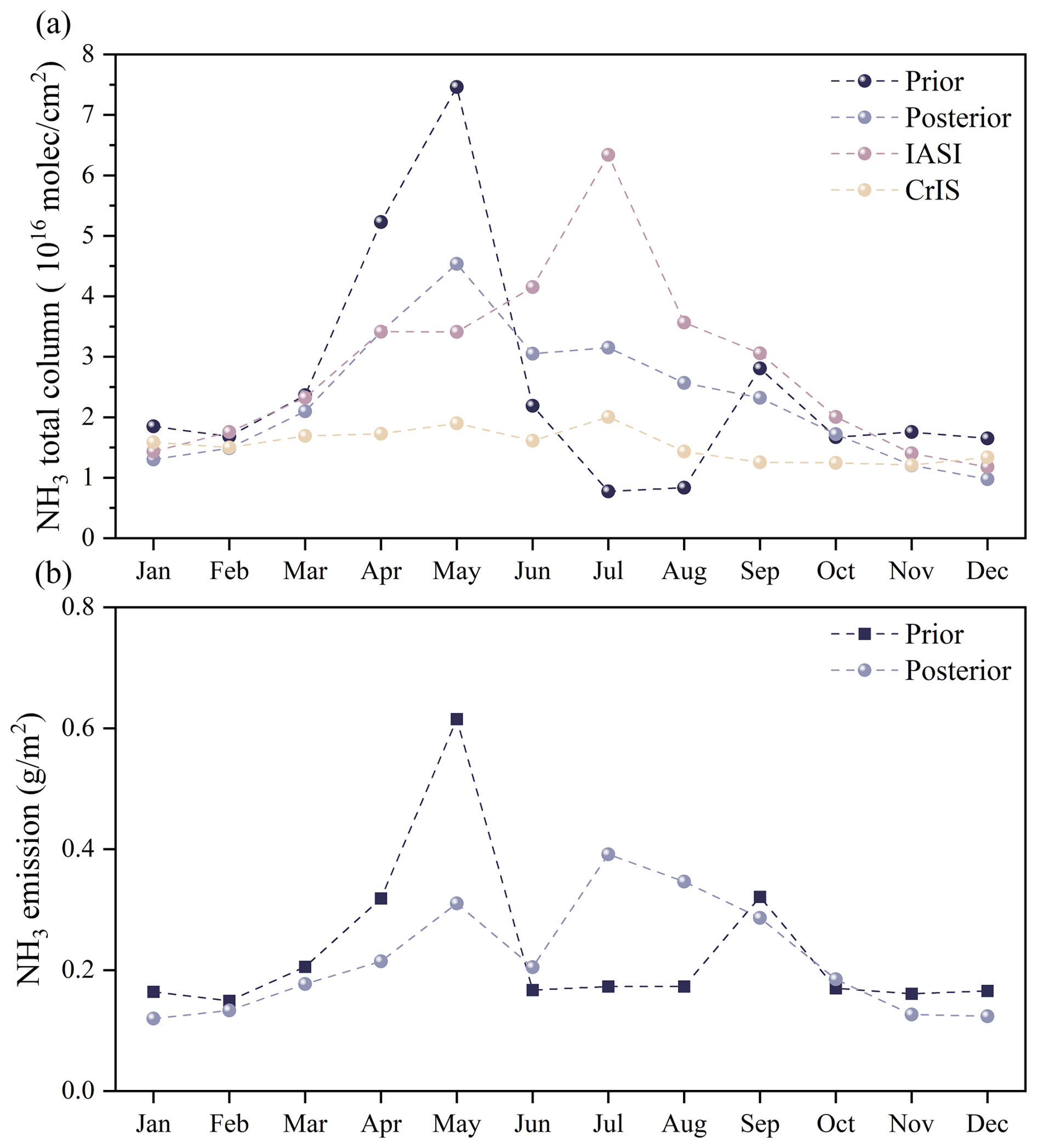
Figure 4 The monthly average total NH₃ column concentrations from the prior and posterior, observed by IASI and CrIS from January to December (a). The monthly average values of the prior and posterior emissions from January to December (b).

Figure 5a–i illustrates the annual average NH₃ column concentrations observed by the IASI satellite instruments from 2015 to 2023. The data clearly show that Pakistan and northern India consistently experience the highest NH₃ concentrations, with values exceeding 5 × 10¹⁶ molec. cm⁻². Furthermore, the spatial distribution of annual average NH₃ column concentrations remained relatively stable over the past decade.

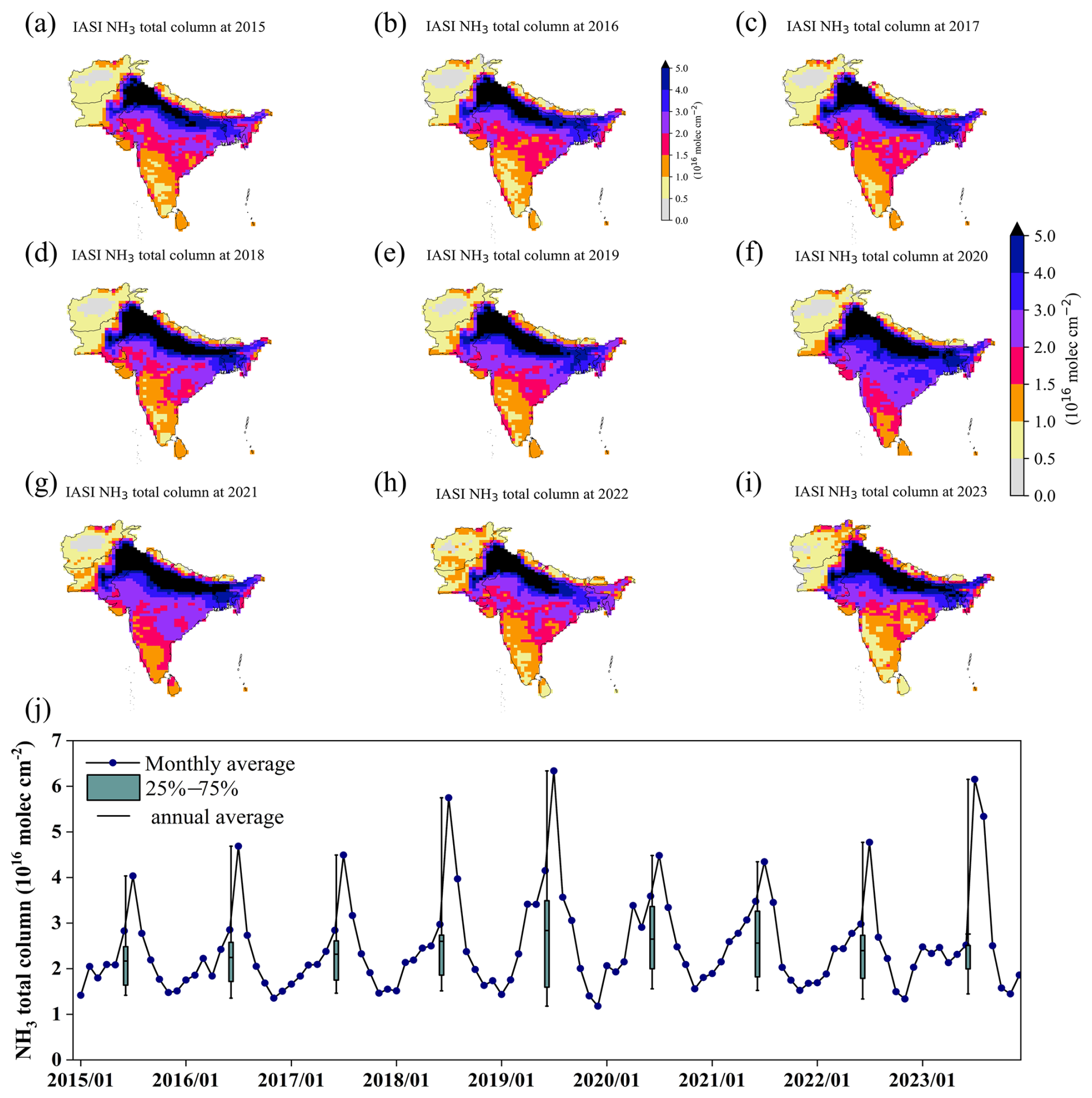
Figure 5 The spatial distribution of the annual averaged IASI column concentrations in South Asia from 2015 to 2023 (a–i). Panel (j) presents a time series depicting the monthly variation in IASI-observed NH₃ column concentrations from 2015 to 2023, with the box plots representing the yearly averages, showing interannual changes.

Figure 5j depicts the monthly mean NH₃ column concentrations derived from the IASI satellite. The time series reveals a clear seasonal pattern, with peaks occurring in summer and lower levels in winter, and shows that the highest concentrations were consistently observed in July. Additionally, the inter-annual variation in NH₃ column concentrations from 2013 to 2019 exhibits a modest upward trend, ranging from 2.17 to 2.6 (× 10¹⁶ molec. cm⁻²), corresponding to an average growth rate of approximately 6.32 %. Subsequent to 2019, NH₃ concentrations stabilize within the range of 2.6 to 2.8 (× 10¹⁶ molec. cm⁻²). Given the relatively stable NH₃ levels after 2019, we restricted our analysis to conducting an assimilation-based emission inversion for the year 2019. Extending emission inversion over a longer period would require substantial computational resources.

3.2 Anthropogenic NH₃ emissions analysis

By assimilating IASI NH₃ column concentrations, the posterior anthropogenic monthly NH₃ emission inventories for 2019 were updated. Scenarios of the posterior emission inventories, along with the increments (posterior minus prior), for January, April, July, and November are shown in Fig. 3b–c. The prior, posterior, and increment data for the remaining months of 2019 are provided in Figs. S7–S9 in the Supplement. Our posterior inventory demonstrated that, in general, the primary sources of NH₃ originated from North India, Pakistan, and Bengal. This finding is consistent with the CEDS inventory, as well as with other studies (Pawar et al., 2021). However, a huge discrepancy emerged when we compared the posterior and prior results, particular for April (in Fig. 3b) and July (in Fig. S3c). The posterior results reveal a distinct seasonal emission profile compared to the prior. Specifically, emissions during spring are significantly overestimated by the prior model, whereas summer emissions are underestimated by up to 3-fold.

To better illustrate the differences in timing profiles throughout the year, the monthly average emission intensity over South Asia was calculated and is shown in Fig. 4b. The prior anthropogenic emission inventory exhibits a “double-peak” pattern, mirroring the profile of the average NH₃ concentration displayed in Fig. 4a. The emission flux reaches its maximum in May, peaking at approximately 0.6 g m⁻², with a secondary peak occurring in September around 0.25 g m⁻². In contrast, the assimilation that integrates prior CEDS emissions with IASI measurements shows much lower intensities from January to May, with the largest negative differences (>0.3 g m⁻²) observed in May. While the prior emissions remain relatively low during the summer, the emission inversion reveals positive increments, with the posterior inventory indicating the maximum emission flux in July, peaking at approximately 0.4 g m⁻². In general, the posterior emissions also display a “double-peak” pattern; however, the peaks occur in May and July, in contrast to the May and September peaks observed in the prior emissions.

The substantial emissions in July, as indicated by the posterior anthropogenic inventory, can be attributed to the increased fertilizer application for crops during the summer season (Tanvir et al., 2019). As shown in Table 2, the sowing period for crops in South Asia is generally from May to July, with July being the peak growth period for crops, resulting in a large amount of fertilization, resulting in July surpassing May in emission intensity. From July to September, as rice and other crops progress through their growth stages, fertilizer application typically decreases, leading to a gradual reduction in NH₃ emissions. Additionally, temperatures decline from August to September Fig. S6b, reducing the volatilization rate of NH₃, thereby leading to a further decrease in emissions. This pattern occurs because NH₃ volatilization is strongly influenced by temperature (Fan et al., 2011).

The convergence of prior and posterior anthropogenic emission intensities in June is attributed to the overall offsetting of negative and positive increments in the region, as shown in Fig. S9f. As depicted in panel (c) of Fig. 3, the negative increments observed in January and April primarily originate from the Indian region, while the positive increments in July and September are predominantly observed in the same area. Additionally, the posterior emission estimates, which are based on CrIS, have now been included.

3.3 Validation

To evaluate our inversion results, we compared the atmospheric NH₃ simulation driven by either the posterior emission (referred to as the posterior simulation) or the prior one against the observations, including the assimilated IASI column data and the independent CrIS retrieval and ground-based NH₃ and PM_2.5 concentration measurements.

3.3.1 NH₃ total column concentration validation

The difference between the model and IASI observations for the entire year of 2019 is shown in Fig. 6a. The overestimation by the prior model is particularly evident in spring (especially May), while the underestimation is most prominent in summer (especially July). These discrepancies contributed to a relatively high model error, with the correlation coefficient (R) as low as 0.33 and the root mean square error (RMSE) as high as 4.64 × 10¹⁶ molec. cm⁻². In contrast, the posterior emission-driven GEOS-Chem simulations showed good consistency with the IASI retrievals, capturing both the spatial and temporal variations, as shown in panel (d) of Fig. 1. This resulted in significantly improved performance, with R increasing to 0.76 and RMSE reducing to 2.48 × 10¹⁶ molec cm⁻², as shown in panel (b) of Fig. 6. The discrepancy between the model and the posterior results mentioned in Sect. 3.1.1 in July is also evident in the scatter plot of the posterior column simulation against the IASI measurements in panel (b) of Fig. 6.

In addition, we further evaluated our posterior simulations using the other advanced satellite NH₃ product from the CrIS instruments. The scatter plots of the CrIS monthly NH₃ column concentrations vs. the prior/posterior simulations in 2019 are presented in panels (c) and (d) of Fig. 6. Steady improvements were observed in the comparison against the independent CrIS retrievals, with the correlation coefficient (R) increasing from 0.42 to 0.71 and the RMSE decreasing from 3.96 to 2.06 × 10¹⁶ molec. cm⁻². These evaluations give us confidence that our emission inversion has successfully calculated the most likely posterior, given both the prior and the IASI measurements.

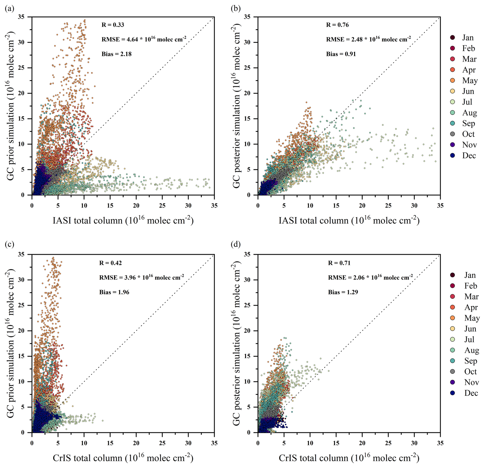
Figure 6 Scatter plot of the IASI (a–b) and CrIS (c–d) observed NH₃ concentrations against the NH₃ simulation over South Asia, using either the prior or the posterior NH₃ emission inventory, from January to December.

3.3.2 NH₃ and PM_2.5 ground concentration validation

The few surface NH₃ concentration observations from ground stations, shown in Fig. 2, were also utilized to evaluate our NH₃ emission inversion results. Figure 7 presents the scatter plot of monthly surface NH₃ concentrations against the prior/posterior simulations. Our posterior results are in better agreement with these independent surface NH₃ concentration measurements. This is evident from the higher correlation coefficient (R=0.39) in the posterior compared to R=0.28 in the prior simulation. The RMSE values remained almost the same, changing slightly from 22.18 µg m⁻³ in the prior to 22.73 µg m⁻³ in the posterior. The large remaining error is due to several instances where ground NH₃ concentration measurements indicated values several times higher than our simulations. This was also reported by Pawar et al. (2021), which suggests that ground NH₃ observations are likely to overestimate NH₃ levels. The mismatch between ground observations and simulations may be attributed to the fact that most monitoring stations are located in urban regions of India, where NH₃ concentrations are higher due to traffic and human activities (Sharma et al., 2014). Simulations with an extremely fine resolution could provide a more accurate representation of NH₃ characteristics at these surface sites. However, such simulations would significantly increase the computational burden on the emission inversion system, which is beyond the scope of this study.

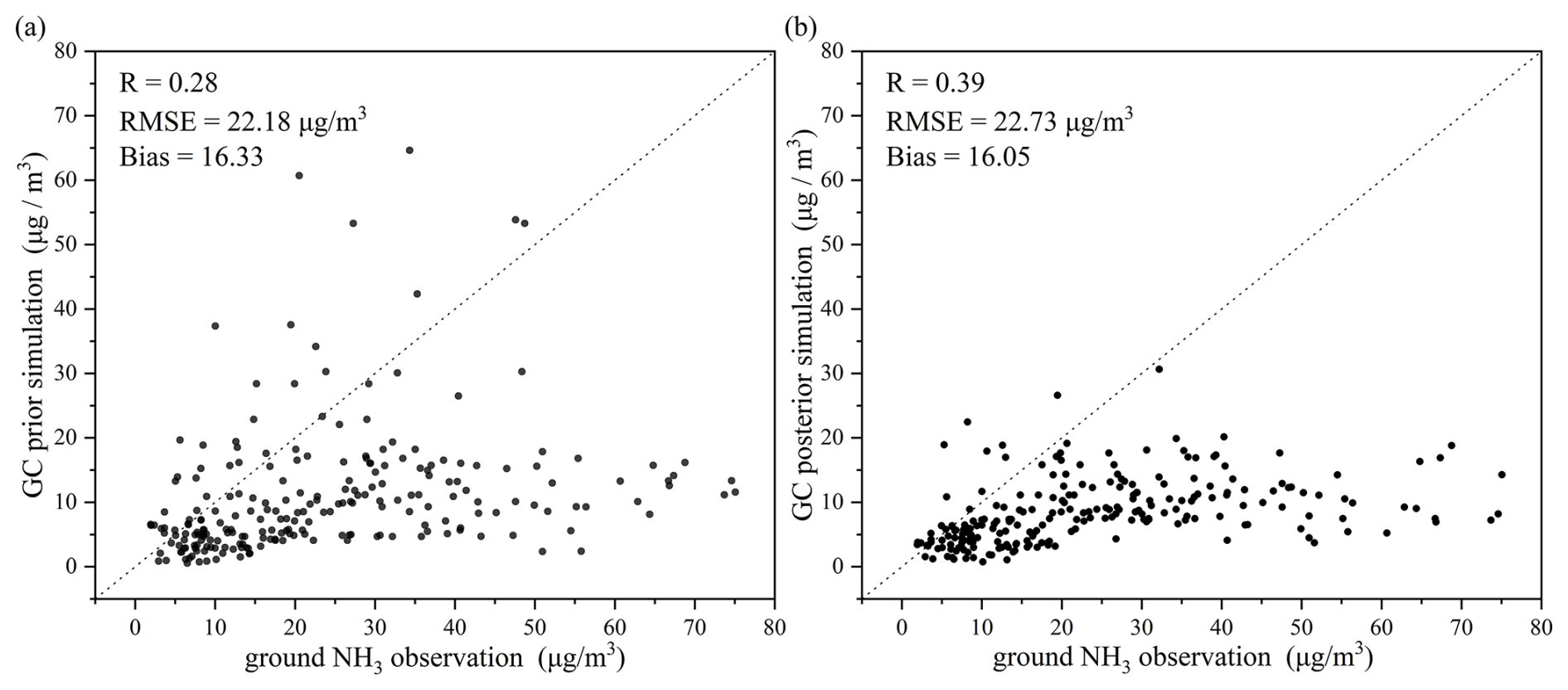
Figure 7 Scatter plot of the ground-observed vs. NH₃ simulation over South Asia using either the prior (a) or the posterior (b) NH₃ emission inventory for 2019.

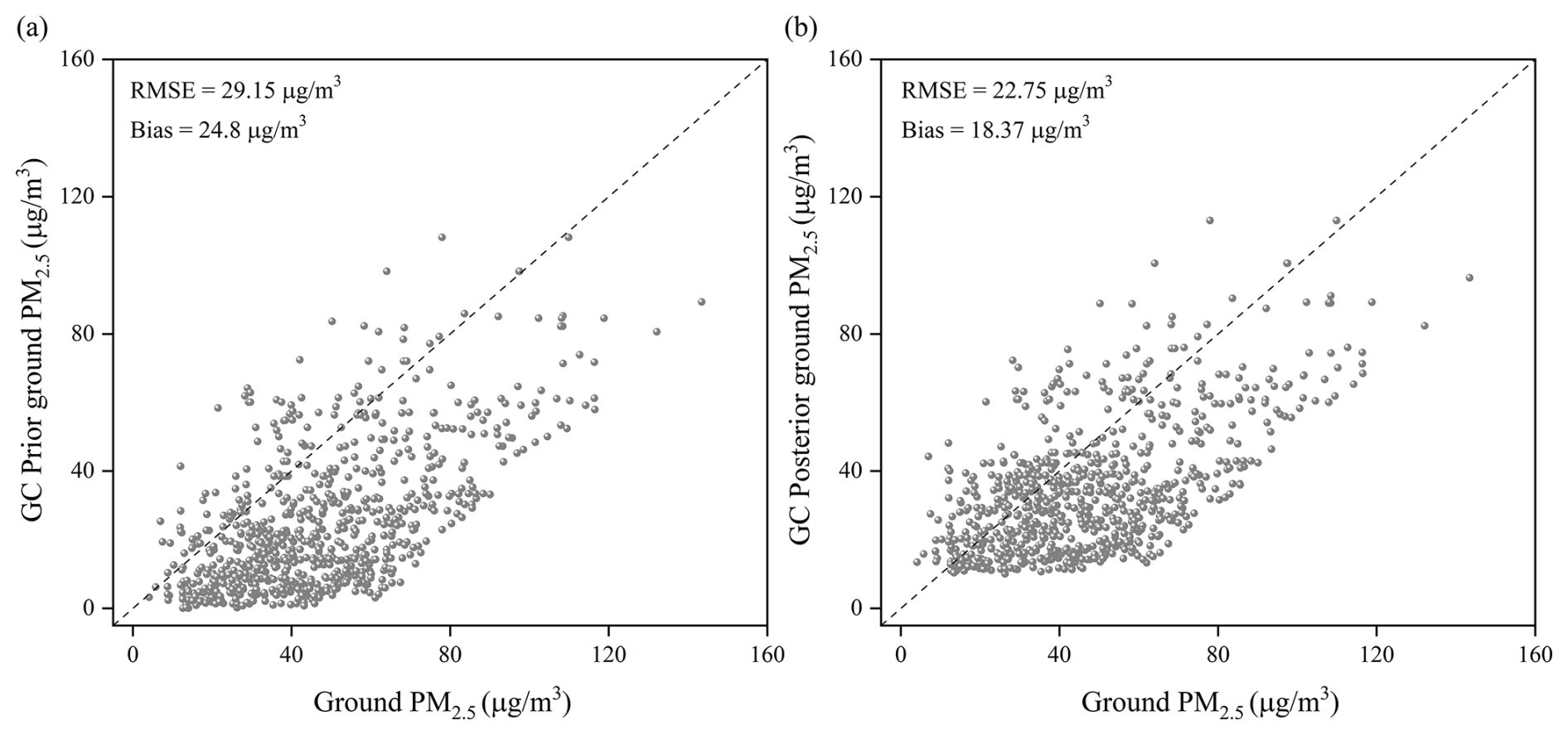
Figure 8 Scatter plot of the ground-observed vs. PM_2.5 simulation over South Asia using either the prior (a) or the posterior (b) emission inventory for 2019.

NH₃ is the key precursor of the inorganic aerosol. The estimated NH₃ emission inventory is supposed to improve the aerosol simulation as well, under the assumption that aerosols from other sources are accurately represented. The monthly averaged PM_2.5 concentrations against the simulations using either our prior or the posterior NH₃ inventory, as shown in Fig. 8a–b. It is evident that both RMSE and Bias have been reduced to varying degrees: RMSE decreased from 29.15 µg m⁻³ in the prior to 22.75 µg m⁻³ in the posterior, and bias decreased from 24.8 µg m⁻³ in the prior to 18.37 µg m⁻³ in the posterior. These results indicate that the emission inventory optimized by our inversion system has improved the model's performance in simulating PM_2.5, reducing both systematic biases and model underestimation effectively.

4 Summary and conclusion

South Asia has been severely affected by NH₃, which has significant impacts on both human health and the ecological environment. The current emission inventories, primarily based on bottom-up approaches, are subject to substantial uncertainties. This is due to the fact that the intensity of NH₃ emissions from livestock and fertilizers is heavily influenced by management and farming practices, yet this information is often not widely available. As a result, accurately simulating the spatiotemporal characteristics of atmospheric NH₃ and evaluating its impacts remain challenging. The use of satellite observations, such as those from IASI, for top-down emission inversion has emerged as an effective method to develop more accurate inventories. However, research in this area remains limited in South Asia.

This study employed a 4DEnVar-based emission inversion system to optimize anthropogenic NH₃ emissions in South Asia. The most likely posterior monthly anthropogenic NH₃ emission inventories were calculated given the CEDS prior inventory and the NH₃ column concentration observations from the polar-orbiting IASI satellite instrument. Validation against satellite and ground-based observations shows that NH₃ concentration simulations driven by the posterior emissions perform significantly better than those driven by the prior inventory. In the comparison against the IASI measurements, the correlation coefficient (r) increased from 0.33 (for the prior) to 0.76, and the root mean square error (RMSE) was reduced from 4.64 × 10¹⁶ molec. cm⁻² (prior) to 2.48 × 10¹⁶ molec. cm⁻² (posterior). The posterior results also show improvements when compared to independent CrIS satellite measurements, with the correlation coefficient (r) rising from 0.42 (prior) to 0.71 and RMSE reducing from 3.96 × 10¹⁶  molec. cm⁻² (prior) to 2.06 × 10¹⁶ molec. cm⁻² (posterior). Additionally, validation with ground-level NH₃ and PM_2.5 concentrations further supports the findings, demonstrating that our emission inversion system effectively reduces systematic biases and underestimation in ground-level simulations.

The spatial and temporal characteristics of anthropogenic NH₃ emissions over South Asia were then analyzed based on the inversion. While the prior CEDS inventory generally captured the NH₃ emission hotspots, such as in Pakistan, North India, and Bengal, it failed to accurately represent the seasonal trend. Specifically, the prior inventory showed a “double-peak” pattern throughout the year, with peaks in May and September. In contrast, the posterior results revealed the correct seasonal pattern, with the “double-peak” profile occurring in May and July. The posterior emission inventory's total annual estimate is 12.61 Tg, compared to the prior inventory's 13.32 Tg.

The top-down NH₃ emission inversion system driven by IASI observations has demonstrated superior performance in enhancing the NH₃ emission estimates. Nevertheless, several challenges persist, such as the requirement for simulations at finer resolutions to precisely capture very local emission dynamics. Furthermore, observations from stationary satellites, such as FY-4B, also deserve attention for exploring the diurnal variations of the NH₃ emission. Our next steps will focus on further refining the spatiotemporal patterns at the daily or weekly scale, building on the current posterior results.