Toward a learnable Artificial Intelligence Model for Aerosol Chemistry and Interactions (AIMACI) based on the Multi-Head Self-Attention algorithm

Simulating aerosol chemistry and interactions (ACI) is crucial in climate and atmospheric modeling, yet conventional numerical schemes are computationally intensive due to the stiff differential equations and iterative methods involved. While artificial intelligence (AI) has demonstrated potential in accelerating photochemistry simulations, it has not been applied for simulating the full ACI processes, which encompass not only chemical reactions but also other processes, such as nucleation and coagulation. To bridge this gap, we develop a novel Artificial Intelligence Model for Aerosol Chemistry and Interactions (AIMACI), focusing initially on inorganic aerosols. Trained based on a conventional scheme, it has been validated in both offline and online modes (referring to whether it is coupled into a three-dimensional atmospheric model). Results demonstrate that AIMACI is not only comparable with conventional schemes in spatial distributions, temporal variations, and evolution of particle size distribution of main aerosol species, including water content in aerosols, but also exhibits robust generalization ability, reliably simulating one month under different environmental conditions across four seasons despite being trained on limited data from merely 16 d. Notably, it exhibits ∼5× speedup with a single CPU and ∼277× speedup with a single GPU, compared with conventional schemes. However, the stability of AIMACI for year-scale global simulations remains to be seen, requiring further testing. AIMACI's generalization capability and its modular design suggest potential for future coupling to global climate models, which are expected to enhance the precision and efficiency of ACI simulations in climate modeling that neglects or simplifies ACI processes.

1 Introduction

Atmospheric aerosols, which consist of a suspension of solid and liquid particles in the air, exert a profound influence on Earth's climate system and air quality (Charlson et al., 1992). Their multifaceted impacts are evident in their capacity to alter the Earth's radiation balance through the scattering and absorption of solar and longwave radiation, as well as in their role as cloud condensation nuclei that influence the formation and characteristics of clouds (Twomey, 1974; Lohmann and Feichter, 2005; Bellouin et al., 2020; Li et al., 2022). The presence of atmospheric aerosols extends its reach to environmental well-being, with implications that span visibility, human health, and the integrity of ecological ecosystems (Pöschl, 2005; Arfin et al., 2023). Full aerosol chemistry and interactions (ACI) consist of multiple highly nonlinear subprocesses, including chemical reactions, phase equilibrium, gas-particle partitioning, particle size growth, coagulation, and nucleation, which have a significant impact on the concentration of atmospheric aerosols (Zaveri et al., 2008). Numerical models stand as indispensable analytical tools, pivotal for comprehending the aforementioned phenomena, and are instrumental in air quality management and the formulation of mitigation strategies for climate change. However, simulating full ACI processes within these models poses a significant computational challenge (Carmichael et al., 1999; Ebel et al., 2006). As quantified in Fig. S1, using the Model for Simulating Aerosol Interactions and Chemistry (MOSAIC) scheme with four bins for full ACI simulation in the Weather Research and Forecasting with Chemistry (WRF-Chem) model accounts for 31.4 % of the total computational time of the chemistry module. This is primarily due to the requirement to solve a complex set of stiff nonlinear differential equations governing aerosol processes, coupled with the use of implicit integration schemes to ensure numerical stability (Sandu et al., 1997a, b). Furthermore, to accommodate the diverse methodologies for describing the evolution of particle size distribution (PSD), some aerosol processes may require repeated calculations (J. L. Wang et al., 2022). For example, when employing a discrete model, the coagulation collision frequency functions need to be computed for each discrete size (Zhang et al., 2020). Consequently, the computational burden is significantly amplified. This computational intensity often creates a dilemma, as it competes with other priorities in numerical modeling, such as enhancing spatial resolution (Gu et al., 2022), recognized as helpful for minimizing uncertainties in numerical models. Numerous numerical models opt for simplified or even deactivated ACI schemes during long-term simulations, particularly in high-resolution atmospheric and climate models, introducing considerable uncertainties in the simulation results (Lee et al., 2016; Zhang et al., 2020). Consequently, there is a pressing need to achieve rapid, accurate, and stable simulation of ACI within numerical models.

Over the past few decades, extensive research efforts have been dedicated to striking a tradeoff between accuracy and computational efficiency in simulating ACI. Researchers have primarily approached this challenge from two distinct perspectives: one is the exploration of various methodologies for describing the evolution of PSD. For instance, in the discrete model, the PSD is divided into discrete sizes, with calculations performed for each individual size. This approach yields the most precise results but also demands the highest computational resources (Landgrebe and Pratsinis, 1990; Zhao et al., 2013b). The moment model, which tracks the lower-order moments of an unknown aerosol distribution, is particularly well-suited for scenarios where the size distribution is lognormal (Pratsinis, 1988). Concurrently, researchers have been engaged in employing diverse methodologies to solve the system of stiff differential equations. For example, the Multicomponent Taylor Expansion Method (MTEM) has been developed to compute activity coefficients in aqueous atmospheric aerosols (Zaveri et al., 2005). This method offers an efficient noniterative solution for systems rich in sulfate aerosols. The Adaptive Step Time-split Euler Method (ASTEM) leverages several key characteristics of the atmospheric gas-particle partitioning, systematically reducing stiffness while preserving the integrity of the numerical solution (Zaveri et al., 2008). Despite these advancements significantly improving the computational efficiency of simulating ACI, current progress remains far from sufficient.

An alternative approach is to utilize artificial intelligence (AI) schemes to replace conventional numerical schemes in atmospheric and climate models, which could potentially bring about a transformative impact. Recent studies by Liu et al. (2021) developed an AI scheme based on a Residual Neural Network (ResNet) algorithm for simulating atmospheric photochemistry, achieving a nearly 10.6× increase in computational efficiency. However, they adopted a hybrid approach, combining a numerical scheme for radicals and oxidants with an AI scheme for volatile organic compounds (VOCs). Kelp et al. (2022) employed an online training strategy to refine an AI scheme for a simplified super-fast chemistry scheme (12 species) in atmospheric models, achieving stable simulations over a year with a nearly 5× speedup. However, their approach required training four separate AI emulators for each season and simulation discontinuities (characterized by abrupt changes in simulation errors) were observed when switching between seasonal AI emulators. Sharma et al. (2023) developed a physics-informed AI approach to study isoprene epoxydiols in acidic aqueous aerosols over the Amazon rainforest, halving computational costs but requiring the training of separate AI models for each size bin. Xia et al. (2025) have taken a step further by developing an artificial intelligence photochemistry (AIPC) scheme, leveraging the Multi-Head Self-Attention (MHSA) algorithm to simulate a full complex atmospheric photochemistry (79 species) with a unified AI model. When coupled with three-dimensional (3D) numerical models, their approach not only reliably simulates the continuous spatiotemporal evolution of 79 chemical species over 15 consecutive days but also improves computational efficiency by 77 %.

While these studies have demonstrated AI schemes' capability to capture nonlinear chemical relationships and reproduce complex spatiotemporal distributions, no current AI scheme has achieved fast, accurate, and stable end-to-end simulation of full ACI within 3D atmospheric models. Unlike atmospheric photochemistry, which only involves chemical reactions between species, the full ACI encompasses multiple other intricate processes. Furthermore, since the PSD of an aerosol significantly influences aerosol behavior, an accurate depiction of the evolution of PSD is as critical as the precise simulation of aerosol species concentration. These requirements collectively present a heightened challenge for AI scheme development. Consequently, the fundamental question of whether an AI scheme can effectively replace traditional numerical schemes for full ACI simulation – while simultaneously achieving high fidelity in spatiotemporal distributions and substantial improvements in computational efficiency – remains unresolved in atmospheric modeling research.

To bridge this gap, in this study, we have developed a novel Artificial Intelligence Model for Aerosol Chemistry and Interactions, termed AIMACI, which is based on the Multi-Head Self-Attention algorithm and has been coupled online with a 3D numerical atmospheric model. As a first step, this study primarily focuses on inorganic aerosols because they constitute significant amounts of secondary aerosols globally and serve as the important driver of aerosol radiative forcing and cloud condensation nuclei activity in current climate models. Given that the production of secondary organic aerosols (SOAs) involves significantly more complex chemical pathways, encompassing a wider array of precursor species and heterogeneous reaction mechanisms, the current AIMACI does not include them. Their incorporation will be considered in the future development of AIMACI. To validate the accuracy, stability, and computational efficiency of the AIMACI scheme, we conducted a series of experiments for both offline simulations (where the AIMACI scheme was not coupled to a numerical model) and online simulations (where the AIMACI scheme was coupled to a numerical model). The structure of this paper is organized as follows: Sect. 2 provides a detailed description of the WRF-Chem model and the establishment of the AIMACI. Section 3 discusses the results, and Sect. 4 presents the conclusion, outlining the implications of our findings for the field.

2 Methods

2.1 WRF-Chem model and MOSAIC scheme

In this study, we utilize the updated version of WRF-Chem developed by the University of Science and Technology of China (USTC) for conducting all simulations. This USTC version of WRF-Chem boasts additional functionalities compared with the publicly released version, including the capability to diagnose radiative forcing of aerosol species, land-surface-coupled biogenic volatile organic compound emissions, and aerosol–snow interactions (Du et al., 2020; Hu et al., 2019; Zhang et al., 2021; Zhao et al., 2013a, b, 2014, 2016).

The conventional numerical scheme adopted in this study for full ACI simulation is the MOSAIC scheme (Zaveri et al., 2008), coupled with the CBM-Z (Carbon Bond Mechanism version Z) photochemistry scheme (Zaveri and Peters, 1999). The MOSAIC scheme stands out for its innovative approach to address the long-standing issues in solving the dynamic partitioning of semivolatile inorganic gases (HNO₃, HCl, and NH₃) to size-distributed atmospheric aerosol particles. It has been validated against a benchmark model version utilizing a rigorous solver for the integration of stiff differential equations, demonstrating both computational efficiency and high fidelity (Zaveri et al., 2008). The MOSAIC scheme used in this study features four discrete size bins (0.039–0.156, 0.156–0.625, 0.625–2.5, and 2.5–10.0 µm in diameter) and treats all the major aerosol species important at urban, regional, and global scales, including sulfate (SO${}_{\mathrm{4}}^{\mathrm{2}-}$), nitrate (NO${}_{\mathrm{3}}^{-}$), chloride (Cl⁻), carbonate (CO${}_{\mathrm{3}}^{\mathrm{2}-}$), ammonium (NH4⁺), sodium (Na⁺), calcium (Ca²⁺), black carbon (BC), organic carbon (OC), other inorganic mass (OIN), mineral dust, methanesulfonic acid (MSA), and liquid water content of aerosol (water). It also considers the impact of marine biogenic sources of dimethyl sulfide on atmospheric aerosols and some aqueous processes. The chemical reactions among various species are detailed in Zaveri et al. (2008). However, secondary organic aerosols (SOAs) and complex heterogeneous chemical processes (e.g., oxidation of dissolved S(IV) by H₂O₂, O₃, NO₂, and O₂ catalyzed by transition metal ions (TMIs) in aerosol water, Ruan et al., 2022) are not included in the chosen MOSAIC scheme in this study. These aspects will be considered in future development.

2.2 Learnable AIMACI scheme

2.2.1 Scheme construction

Previous attempts to substitute conventional numerical schemes with AI schemes have predominantly utilized simple AI algorithms, such as random forest regression (Keller and Evans, 2019). This preference stems from the challenge of coupling sophisticated AI algorithms, often written in Python, with numerical models coded in Fortran. While some studies have explored the use of advanced AI algorithms, such as fully connected neural networks (Sharma et al., 2023) and residual neural networks (Kelp et al., 2018, 2020, 2022; Liu, 2021; Z. Wang et al., 2022), these have occasionally encountered difficulties when dealing with high-dimensional input variables and have demonstrated limitations in accurately simulating highly nonlinear systems (Xia et al., 2025).

In this study, for the first time, we attempt to use an AI algorithm to achieve end-to-end simulation of the full ACI within a 3D atmospheric numerical model, replacing the chosen MOSAIC numerical scheme to improve computational efficiency. Given the complexity of multiple subprocesses involved in full ACI, there is a clear need for AI algorithms with superior representational capacity for nonlinear systems. The Multi-Head Self-Attention (MHSA) mechanism, a pivotal component of state-of-the-art transformer architectures, has demonstrated exceptional performance across diverse domains such as natural language processing (Vaswani et al., 2017), computer vision (Liu et al., 2021), and weather forecasting (Bi et al., 2023). Additionally, in the development of an artificial intelligence photochemistry scheme, Xia et al. (2025) have highlighted that the MHSA algorithm excels in capturing the intricate chemical relationships among different species through calculating attention weights. Not only does it offer high accuracy and computational efficiency but it is also less susceptible to the increase in the number of chemical species. Building upon these advancements, this study leverages the MHSA algorithm to develop an Artificial Intelligence Model for Aerosol Chemistry and Interactions (AIMACI).

Figure 1 illustrates the development strategy of the AIMACI scheme and its integration into our hybrid atmospheric model with physics and AI schemes (physics-AI hybrid model). The corresponding pseudocode schematic diagram for replacing the traditional numerical scheme with the AIMACI scheme in WRF-Chem is provided in Fig. S2. The AI model architecture shown in Fig. 1 is designed with three main components, each serving a distinct function in the simulation process:

1. Input embedding layer. This initial layer receives meteorological variables and chemical species as input features. The input embedding layer is designed as a fully connected layer, which maps the input data into a higher-dimensional space where interdependencies between variables can be more effectively captured.

2. Integrator. As the core of the AI model, it is composed of two identical blocks, each of which contains two sublayers: an attention layer and a feed-forward layer. We apply residual connections around each of these two sublayers, followed by layer normalization. This integrator is responsible for learning the complex and high nonlinear processes of ACI within the data and integrating them over time.

3. Output representation layer. Following the integrator, it is also implemented as a fully connected layer. This layer translates the processed information from the integrator into chemical concentrations, providing the output targets for the simulation.

Furthermore, the AI model is complemented by pre-processing and post-processing steps, such as min-max normalization, to constitute the comprehensive AIMACI scheme. The trained AIMACI scheme was packaged into a static (or dynamic) library and then coupled into WRF-Chem, utilizing TorchScript and LibTorch tools officially provided by PyTorch. Compared with coupling approaches relying on third-party libraries, such as CFFI (C Foreign Function Interface for Python), our method demonstrates two distinct technical advantages:

1. Enhanced computational efficiency. TorchScript and LibTorch, as core components of the PyTorch ecosystem, are specifically optimized for AI model deployment in C$++$ environments. This optimization reduces computational overhead compared with generic third-party libraries.

2. Streamlined implementation. PyTorch's official documentation provides standardized workflows for serializing trained AI models into static or dynamic libraries via TorchScript and LibTorch.

In contrast, third-party libraries lack native support for AI model deployment, necessitating manual reimplementation of low-level interfaces. Therefore, our coupling approach minimizes alterations to the original codebase and offers a lightweight, adaptable, and modular solution. It is capable of encapsulating a wide range of complex AI algorithms and coupling them with atmospheric and climate models.

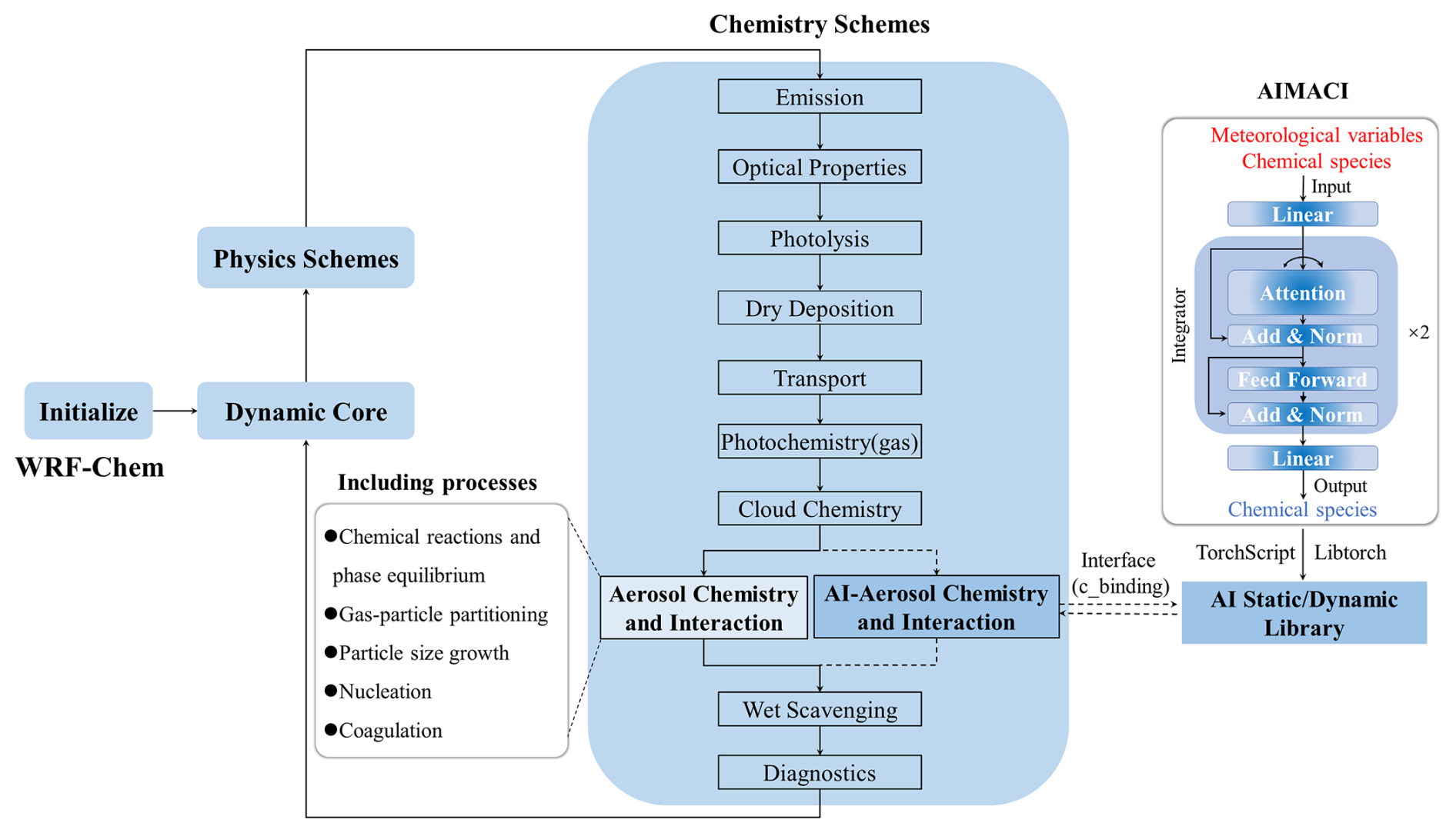
Figure 1 The Artificial Intelligence Model for Aerosol Chemistry and Interactions (AIMACI) in Weather Research and Forecasting with Chemistry (WRF-Chem). The trained AIMACI is packaged into a static/dynamic library using TorchScript and LibTorch, and can be called by WRF-Chem through an interface to replace the numerical scheme for simulating aerosol chemistry and interactions, while the remaining processes maintain the original numerical scheme.

2.2.2 Training and testing procedure

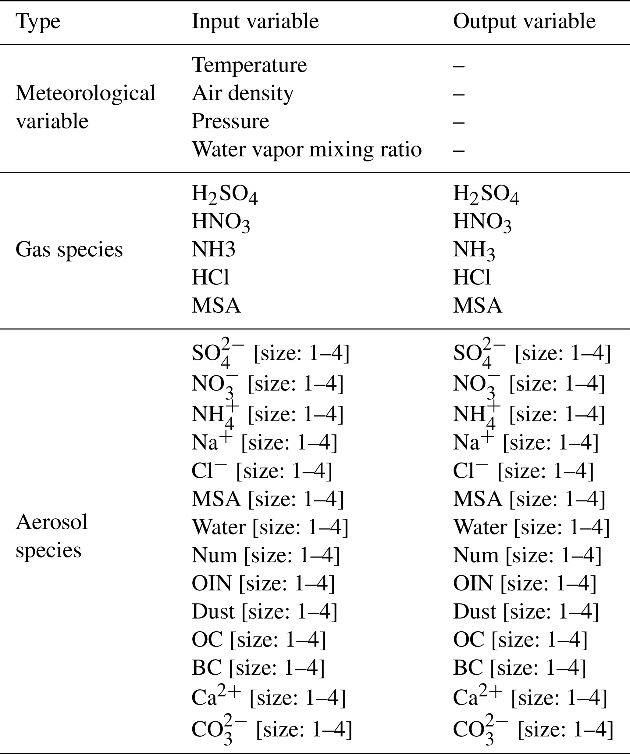
To generate the training, validation, and test datasets, we conducted the WRF-Chem simulations over East China, spanning the period from 1 March 2019 00:00 UTC to 19 March 2019 23:00 UTC. The simulation result was segmented as follows: the initial 16 d, from 2 March 2019 00:00 UTC, were designated as the training set; the penultimate day served as the validation set; and the final day constituted the test set. The simulation was configured with a 0.2° horizontal resolution, covering 140 × 105 grid cells within the geographical bounds of 107.1 to 127.9° E and 19.7 to 47.5° N, and featured 49 vertical layers extending up to 50 hPa. A dynamic time step of 2 min and a chemical time step of 1 h were employed. For emission and meteorological fields, we used the Multi-resolution Emission Inventory for China (MEIC) at 0.25°×0.25° resolution for 2019 (Li et al., 2017; Geng et al., 2024), and the NCEP final reanalysis (FNL) data (NCEP, 2000) with a 1°×1° resolution and 6 h temporal resolution within the simulation domain. Concentrations of aerosol and gas species pertinent to gas-particle partitioning were recorded hourly, along with key meteorological variables influencing chemistry: temperature, pressure, air density, and water vapor mixing ratio. A comprehensive list of variables used for training the AIMACI scheme is presented in Table 1. Due to computational cost considerations, the period of the training dataset is not very long; however, the volume of training samples is large due to the hourly chemical time step and the fine spatial resolution of our simulation. With 140 by 105 grid cells, 49 vertical layers, and 24 h in a day, the total number of training samples amounts to 276 595 200 (140 × 105 × 49 × 24 × 16), reaching the hundred million scale. This large dataset provides a rich and diverse set of samples for training, ensuring that the AI model does not suffer from a lack of convergence due to insufficient data.

In the training of the AI model we built from scratch, each training sample included 65 input features (4 meteorological variables, 5 gas species, and 14 aerosol species with 4 size bins) and 61 output targets (5 gas species and 14 aerosol species with 4 size bins). All features and targets underwent min-max normalization to standardize the data. We employed the PyTorch deep learning framework for model training, with a batch size of 2048, an initial learning rate of 0.001, and the Adam optimization algorithm. The mean squared error (MSE) was used as the loss function. To optimize the training process, we implemented a learning rate decay strategy using the ReduceLROnPlateau scheduler, along with an early stopping mechanism after 10 consecutive epochs without improvement in the validation loss. All other hyperparameters not mentioned are kept at their default values. For this study, we trained the model using three GPUs for approximately 1 d, and the model achieved optimal performance at epoch 32.

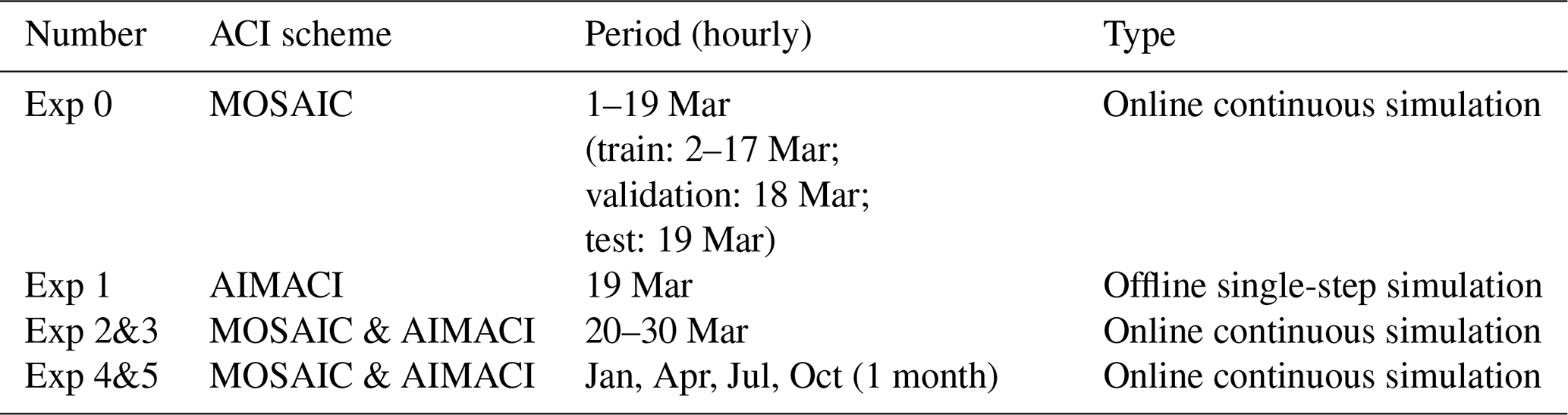
To comprehensively evaluate the performance of the trained AIMACI scheme, we conducted a series of additional experiments in both offline and online modes, as detailed in Table 2. These experiments included the following:

1. Offline simulations were performed on the test dataset without coupling the AIMACI scheme into WRF-Chem, treating AIMACI as a standalone box model to assess its single-step performance.

2. Online simulations were conducted for a 10 d continuous period outside the training phase, following the coupling of the AIMACI scheme into WRF-Chem, where it is invoked at each chemical time step and interacts with other model processes to create a dynamic and iterative aerosol simulation.

3. A month-long online continuous simulation was carried out under different environmental conditions across all four seasons to evaluate the AIMACI scheme's generalization ability.

In order to quantify the performance of the AIMACI scheme, we evaluated statistical indicators for all species and a focused examination of spatial distributions, temporal series, and the evolution of particle size distribution (PSD) for four representative aerosol species. The four selected species are sulfate, nitrate, liquid water content in aerosols, and aerosol number concentration. Sulfate, mainly from fossil fuel emissions, contributes to acid rain, aerosol formation, and aerosol–cloud interactions (Calvert et al., 1985; Fuzzi et al., 2015; Penkett et al., 1979). Nitrate, formed from nitrogen oxides, is a key aerosol component that affects air quality and ecosystems (Parrish et al., 2012; Saiz-Lopez et al., 2017). Liquid water content in aerosols is important for understanding how particles contribute to cloud formation and precipitation (Hodas et al., 2014; Liu et al., 2019; Nguyen et al., 2016; Wu et al., 2018). Aerosol number concentration serves as a key metric for assessing aerosol loading and its direct impact on visibility, radiation balance, and climate feedback mechanisms (Spracklen et al., 2010). Collectively, these four species offer a holistic perspective on the multifaceted role of aerosols in atmospheric processes.

Table 1 Input and output variables of Artificial Intelligence Model for Aerosol Chemistry and Interactions (AIMACI).

Table 2 Numerical experiments conducted in this study.

2.3 Evaluation metric

In this research, a comprehensive evaluation of the AIMACI scheme's effectiveness was conducted utilizing five recognized statistical measures. For every species examined, calculation of the Pearson correlation coefficient (R²), the root mean square error (RMSE), the normalized mean bias (NMB), the absolute error (AE), and relative error (RE) was performed:

$$\begin{array}{}\text{(1)}& {\displaystyle }\uparrow \left(R^{\mathrm{2}}\right)& {\displaystyle }={\displaystyle \frac{{\left({\sum }_{i=\mathrm{1}}^{N_{\mathrm{lat}}}{\sum }_{j=\mathrm{1}}^{N_{\mathrm{long}}}L\left(i\right)\left(c_{i,j}-\stackrel{\mathrm{‾}}{c}\right)\left({\widehat{c}}_{i,j}-\stackrel{\mathrm{‾}}{\widehat{c}}\right)\right)}^{\mathrm{2}}}{\begin{array}{c}{\sum }_{i=\mathrm{1}}^{N_{\mathrm{lat}}}{\sum }_{j=\mathrm{1}}^{N_{\mathrm{long}}}L\left(i\right){\left(c_{i,j}-\stackrel{\mathrm{‾}}{c}\right)}^{\mathrm{2}}\\ \times {\sum }_{i=\mathrm{1}}^{N_{\mathrm{lat}}}{\sum }_{j=\mathrm{1}}^{N_{\mathrm{long}}}L\left(i\right)({\widehat{c}}_{i,j}-\stackrel{\mathrm{‾}}{\widehat{c}}{)}^{\mathrm{2}}\end{array}}},\text{(2)}& {\displaystyle }\downarrow \mathrm{RMSE}& {\displaystyle }=\sqrt{{\displaystyle \frac{{\sum }_{i=\mathrm{1}}^{N_{\mathrm{lat}}}{\sum }_{j=\mathrm{1}}^{N_{\mathrm{long}}}L\left(i\right){\left({\widehat{c}}_{i,j}-c_{i,j}\right)}^{\mathrm{2}}}{N_{\mathrm{lat}}\times N_{\mathrm{long}}}}},\text{(3)}& {\displaystyle }\downarrow \mathrm{NMB}& {\displaystyle }={\displaystyle \frac{{\sum }_{i=\mathrm{1}}^{N_{\mathrm{lat}}}{\sum }_{j=\mathrm{1}}^{N_{\mathrm{long}}}L\left(i\right)\left({\widehat{c}}_{i,j}-c_{i,j}\right)}{{\sum }_{i=\mathrm{1}}^{N_{\mathrm{lat}}}{\sum }_{j=\mathrm{1}}^{N_{\mathrm{long}}}L\left(i\right)c_{i,j}}},\text{(4)}& {\displaystyle }\downarrow \mathrm{AE}& {\displaystyle }=\widehat{C}-C,\text{(5)}& {\displaystyle }\downarrow \mathrm{RE}& {\displaystyle }={\displaystyle \frac{\widehat{C}-C}{C}}.\end{array}$$

In these equations, $L\left(i\right)=N_{\mathrm{lat}}\times \cos {\mathit{\phi }}_i/{\sum }_{i=\mathrm{1}}^{N_{\mathrm{lat}}}\cos {\mathit{\phi }}_i$ is the weight at latitude φ_i, N_lat is the number of grid points in the latitudinal direction, N_long is the number of grid points in the longitudinal direction, $\widehat{C}$ denotes the concentration simulated by the AIMACI scheme, C denotes the concentration simulated by the MOSAIC scheme, ↑ denotes higher values are better, ↓ denotes lower values are better.

2.4 Computational configuration

A primary incentive for coupling AI schemes into atmospheric and climate models is the pursuit of substantial computational acceleration. However, such acceleration is not inherently guaranteed, as demonstrated by Keller and Evans (2019). Consequently, it is imperative to meticulously compare the temporal expenditure of AI schemes against those of traditional numerical schemes.

In this study, we undertook a comparative analysis of the computational time required by the numerical scheme and the AIMACI scheme for simulating ACI in 720 300 discrete grid cells, which roughly corresponds to a global simulation at 2.5° × 2.5° horizontal resolution with 72 vertical layers. To ensure a holistic and unbiased assessment of the speedup achieved, we measured the computational time by averaging the duration of 24 consecutive daily simulations. Both schemes were tested utilizing a single CPU core; we additionally evaluated the AIMACI scheme with a GPU-accelerated scenario using a single GPU. The computational hardware employed in our tests consisted of an Intel-Xeon-E5-2680 2.40 GHz CPU core and an NVIDIA A100-80G GPU.

3 Results

3.1 Offline single-step simulations with the AIMACI scheme

Before coupling the AIMACI scheme with the 3D numerical model WRF-Chem for continuous simulation, we first evaluated its performance on a test dataset that was separate from the training data. The test dataset, as detailed in previous sections, comprises a series of 3D spatial outcomes taken at 24 hourly intervals, on 19 March 2019. It provides representative samples that span a wide range of meteorological conditions and species concentrations. The evaluation on this dataset provides insight into the AIMACI scheme's performance in various atmospheric conditions. Table 3 presents the statistical metrics for all simulated species, offering a comprehensive assessment of the scheme's simulation capabilities.

Quantitative evaluation across 61 output targets demonstrates close alignment between the simulations using the AIMACI scheme and the MOSAIC scheme (hereinafter referred to as the numerical scheme), as evidenced by an average R² of 0.98 and an average NMB of 3.02 %. While 55 output targets, including major inorganic aerosols, such as sulfate, nitrate, and ammonium, achieve R²≥ 0.95, there are still a few species exhibiting relatively poorer statistical metrics, particularly carbonates (Table 3). To delve deeper into this observation, we have plotted the frequency histograms of the concentration distributions for all species in the test data (Fig. S3). Our analysis revealed that species with skewed concentration distributions, particularly those where more than 99 % of the values are close to zero, tend to exhibit poorer statistical indicators. However, this does not signify that the AIMACI scheme has entirely forfeited its predictive capability. As demonstrated in Fig. S4, which illustrates the simulated carbonate concentrations in the 0.625–2.5 µm particle size range (CO₃_a03), the AIMACI scheme continues to perform well in predicting concentration changes in high-value regions. The poorer statistical indicators are primarily attributed to the challenge of accurately forecasting the very low values that are close to zero.

Table 3 Statistical metrics on the test dataset of Artificial Intelligence Model for Aerosol Chemistry and Interactions (AIMACI). (The RMSEs of different species have different units: aerosol (µg kg⁻¹), num (kg⁻¹), gas (ppmv).)

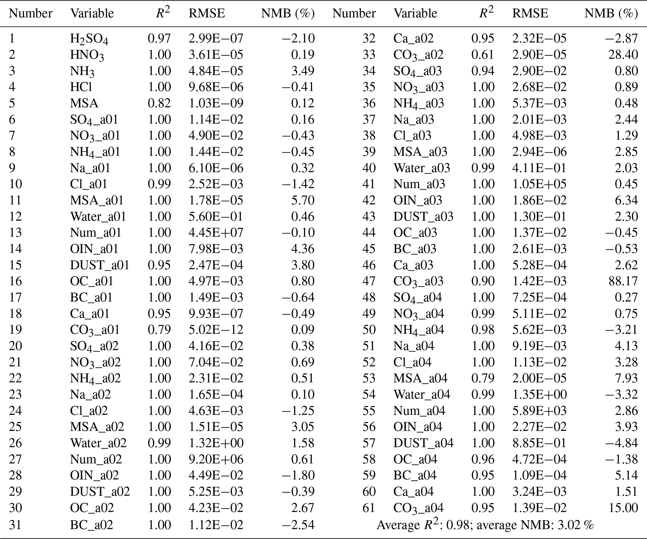
Figure 2 presents the data density and distribution for column concentration of the four key aerosol species selected in Sect. 2.2.2. The results from the numerical scheme simulations indicate that sulfate, nitrate, and liquid water content of aerosol exhibit higher column concentrations within 0.156 to 0.625 µm (size bin 2), whereas the number concentration is notably larger within 0.039 to 0.156 µm (size bin 1). This indicates that, despite the greater number of smaller particles in size bin 1, their overall contribution to the total mass is less significant due to their lower individual mass compared with the larger particles in size bin 2. The AIMACI scheme effectively captures these nuanced aerosol characteristics, as corroborated by the R² of 1.0 depicted in Fig. 2, which underscore the scheme's fidelity in modeling aerosol behavior across various particle sizes.

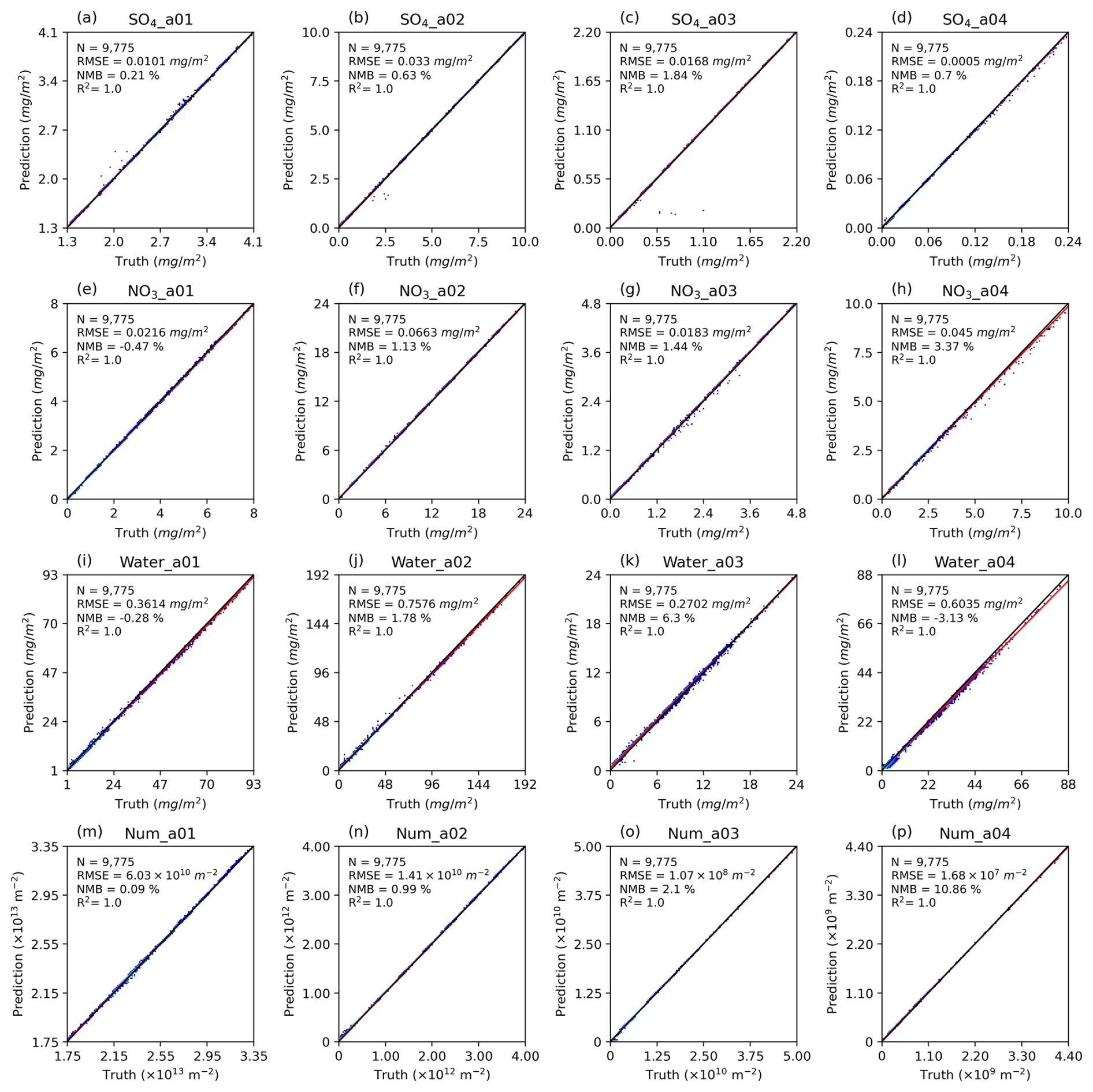
Figure 2 The density plot of column concentration of four key aerosol species (sulfate (SO${}_{\mathrm{4}}^{\mathrm{2}-}$), nitrate (NO${}_{\mathrm{3}}^{-}$), liquid water content of aerosol (water), and number concentration of aerosol (Num)) simulated by the AIMACI scheme on the test dataset. The results are calculated by covering the region spanning from 109.1 to 125.9° E and from 22.1 to 44.9° N, with the data being averaged across the time dimension. The black line is the identical line (y=x), and the red line is the fitted line.

3.2 Online multi-step simulations with the AIMACI scheme

The integration of the AIMACI scheme into 3D atmospheric models to build a physics-AI hybrid model presents unique challenges beyond offline single-step simulation. Online continuous simulation involves not only iterative computation across multiple time steps but also interactions and feedback with numerous other processes in the model. Consequently, a thorough evaluation of the AIMACI scheme's online simulation performance is essential. We focus on its performance across three critical dimensions:

1. Stable and accurate simulation capability. The AIMACI scheme should accurately reproduce the spatiotemporal and size distribution of various aerosol species without rapid accumulation of errors during the simulation process.

2. Robust generalization ability. The AIMACI scheme should be applicable to scenarios beyond the training data, such as different seasons, demonstrating its robustness in a variety of environmental conditions.

3. High computational efficiency. Compared with the conventional numerical scheme, the AIMACI scheme should offer enhanced computational efficiency, which is vital for high-resolution, long-term simulations.

Although these requirements are often challenging to satisfy simultaneously, achieving these benchmarks is crucial for leveraging the full potential of the AIMACI scheme in advancing our understanding of aerosol interactions.

3.2.1 Stable and accurate simulation capability

Coupling AI schemes into numerical models for stable and accurate simulations across multiple time steps has long been a significant challenge. While the simulation errors for individual species at each time step may be minimal, they can accumulate over multiple time steps, and may even spread to other species and physical-chemical processes, leading to chaotic simulation outcomes at the end. Typically, simulations with sophisticated aerosol processes at high resolution, such as those in WRF-Chem, are limited to a few weeks due to computational costs. In this study, we conducted a 10 d continuous simulation from 20 March 2019 00:00 UTC to 30 March 2019 00:00 UTC to evaluate the performance of the AIMACI scheme in a coupled mode.

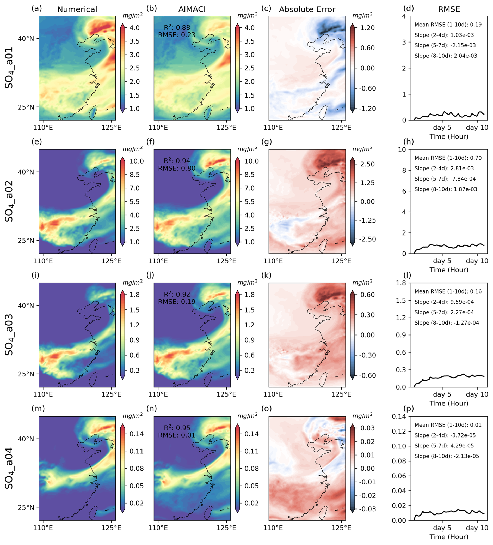
Figure 3 Sulfate column concentration simulations across different size bins. The first and second columns depict the spatial distribution at the 10 d continuous simulation's end (30 March 2019 00:00 UTC), as simulated online by both the numerical scheme and the AIMACI scheme. The third column is the absolute error between them. The fourth column shows the temporal evolution of the hourly RMSE over the 10 d period. The mean RMSE (unit: mg m⁻²) for all days and the slope (unit: mg m⁻² h⁻¹) for different simulation stages (2–4, 5–7, 8–10 d) are given.

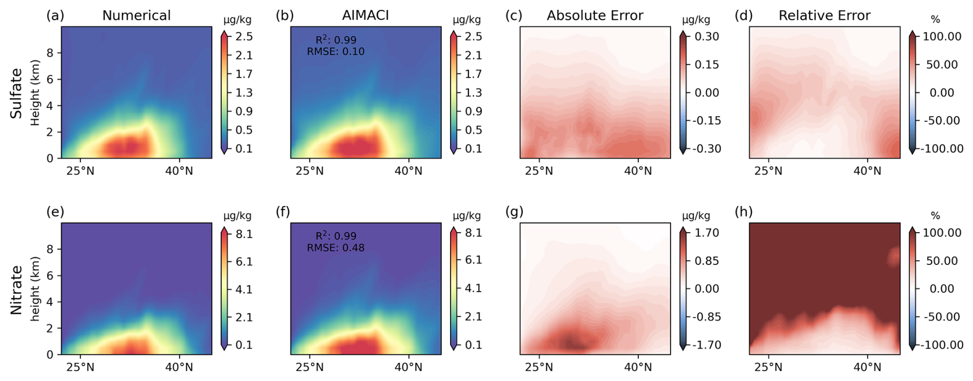
Figure 4 Zonal mean total concentrations (summed across four size bins) of sulfate and nitrate between 109.1 and 125.9° E, as simulated online by both the numerical scheme and the AIMACI scheme. Results are averages over the entire 10 d simulation period.

Figure 3 illustrates the spatial distribution of sulfate column concentrations across different size bins at the end of the 10 d continuous simulation (i.e., 30 March 2019 00:00 UTC), accompanied by the temporal evolution of RMSE during the simulation period. The results reveal that the high-value areas of sulfate column concentrations for different particle sizes exhibit a hook-like structure, extending northeastward from the Yangtze River Economic Belt to the northeastern regions of China. The distinct patterns may be attributed to the complex interplay of meteorological conditions, emission sources, and atmospheric transport processes. The sulfate column concentrations are predominantly concentrated in the range 0.156 to 0.625 µm (size bin 2), with relatively lower column concentrations in the range 2.5 to 10 µm (size bin 4), which is consistent with the findings in Fig. 2. AIMACI reproduces these spatial distribution patterns with strong fidelity, as evidenced by R² exceeding 0.88 across all size bins. However, a systematic bias pattern is observed that, for each particle size, AIMACI tends to underestimate the higher concentration regions and overestimate lower values. This aligns with the findings of Kelp et al. (2022), who report a similar bias pattern in MSE-optimized emulators for photochemistry simulation. We attribute this bias pattern to two main factors: (1) the imbalance in the training dataset, where high-value samples are underrepresented compared with low-value samples, leading to insufficient learning of high-value instances by the AI model; and (2) the use of the RMSE (or MSE) loss function, whose quadratic term penalizes large errors more heavily, thereby biasing the model toward predicting the mean of the target distribution to minimize the overall loss (Gneiting, 2011). While alternative loss functions (e.g., Huber loss) may reduce this bias, RMSE (or MSE) remains widely used in autoregressive simulation studies. One of the key rationales stems from its inherent capability to effectively prevent large errors, which is critical for ensuring the stability of long-term simulations. To alleviate this bias pattern, we plan to explore data transformation techniques to reduce the skewness of the training data distribution in future work. This approach may help alleviate the bias without compromising the stability of the AIMACI.

Additionally, RMSE temporal evolution reveals that, during the entire simulation period, rapid growth is not exhibited and oscillations are maintained within a constrained range. The analysis of the RMSE trend slopes across different simulation stages for four size bins demonstrates nonuniform error progression patterns (e.g., in Fig. 3l, the slope for the 2–4 d period is 0.000959 mg m⁻² h⁻¹, while the slope for the 8–10 d period is −0.000127 mg m⁻² h⁻¹) where, even within identical simulation phases, distinct size bins of the same species manifest divergent error trends (e.g., during the 8–10 d period, the slopes for different size bins are 0.00204, 0.00187, −0.000127, and −0.0000213 mg m⁻² h⁻¹, respectively). The emergence of this complex error variation is related to the dual influence governing each grid point error in online continuous simulations: (1) the inherent limitations of the AIMACI scheme, which achieves accurate simulations when encountering well-learned input feature combinations, while exhibiting degraded performance under insufficiently trained input patterns; and (2) the compound error propagation mechanisms during continuous simulations, where input biases of species concentrations at each time step are affected by three factors – local error accumulation from preceding steps, error propagation through transport processes in numerical models from neighboring grids, and perturbations induced by other processes in numerical models (e.g., dry deposition and wet scavenging). Consequently, input biases exhibit nonlinear variability, with AIMACI's simulation accuracy being inversely correlated to input error magnitudes. In operational implementations of physics-AI hybrid models for online simulations, the influences of these two factors are often interrelated rather than independent, thereby amplifying the complexity of error variation. Introducing an error-correcting operator in the continuous simulation process may enhance the stability of long-term simulations.

Figure 4 presents a comparison of the zonal average total concentrations (summed across all size bins) of sulfate and nitrate, simulated by both the numerical scheme and the AIMACI scheme, with results averaged over the entire 10 d simulation period. Figure 4a and e reveal that high-concentration zones for both sulfate and nitrate are predominantly located between 25 and 40° N, a latitudinal band encompassing the Yangtze River Economic Belt. This spatial distribution is consistent with the region's substantial anthropogenic emissions. Through turbulent mixing and convective transport processes, sulfate and nitrate are vertically transported from lower to higher altitudes, with concentrations exhibiting a characteristic decay profile as altitude increases. Figure 4b and f demonstrate strong agreement between the AIMACI scheme and the numerical scheme, with R² reaching 0.99 for both species. The RMSE further confirms this alignment, measuring 0.10 µg kg⁻¹ for sulfate and 0.48 µg kg⁻¹ for nitrate. The absolute error exhibits a vertical gradient, with larger errors near the surface and smaller errors at higher altitudes. Conversely, the relative error distribution shows an inverse pattern, with lower relative errors near the surface and higher relative errors at elevated altitudes. This behavior arises because species concentrations at higher altitudes are typically below 1.0 µg kg⁻¹, and the relative error calculation divides the absolute error by these low concentration values. Consequently, even small absolute perturbations at high altitudes can result in significantly large relative errors. This effect is particularly pronounced for nitrate, which exhibits concentrations at higher altitudes that are one to two orders of magnitude lower than sulfate, often approaching zero.

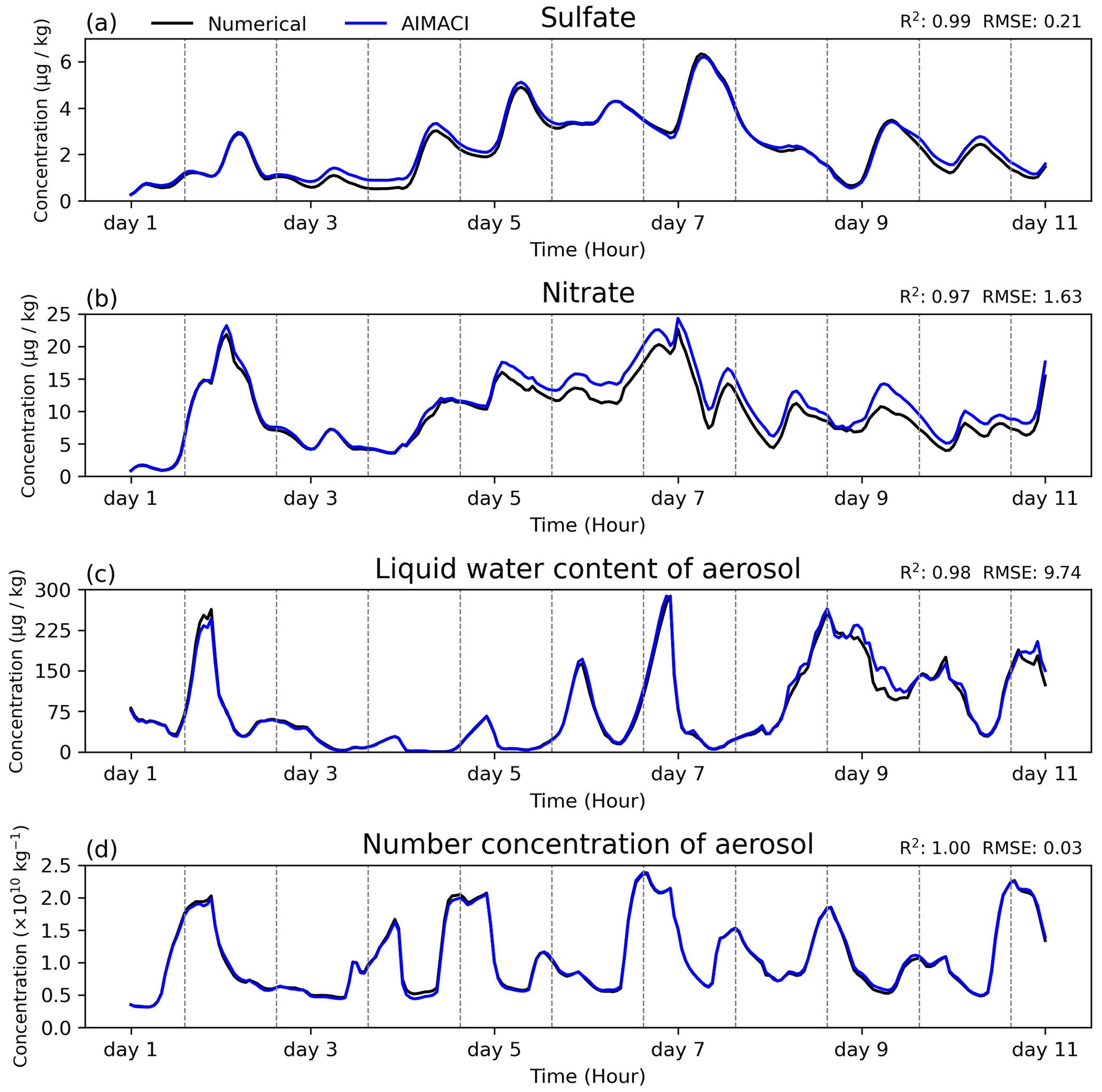
Figure 5 Time series of surface total concentrations (summed across 4 size bins) of four key aerosol species (sulfate, nitrate, liquid water content of aerosol, and number concentration of aerosol), as simulated online by both the numerical scheme and the AIMACI scheme. Results represent the calculated averages for the Yangtze River Delta region (119.1–121.9° E, 30.1–31.9° N). The gray vertical lines mark the time intervals from 0 to 24 h in Beijing Time for each corresponding day.

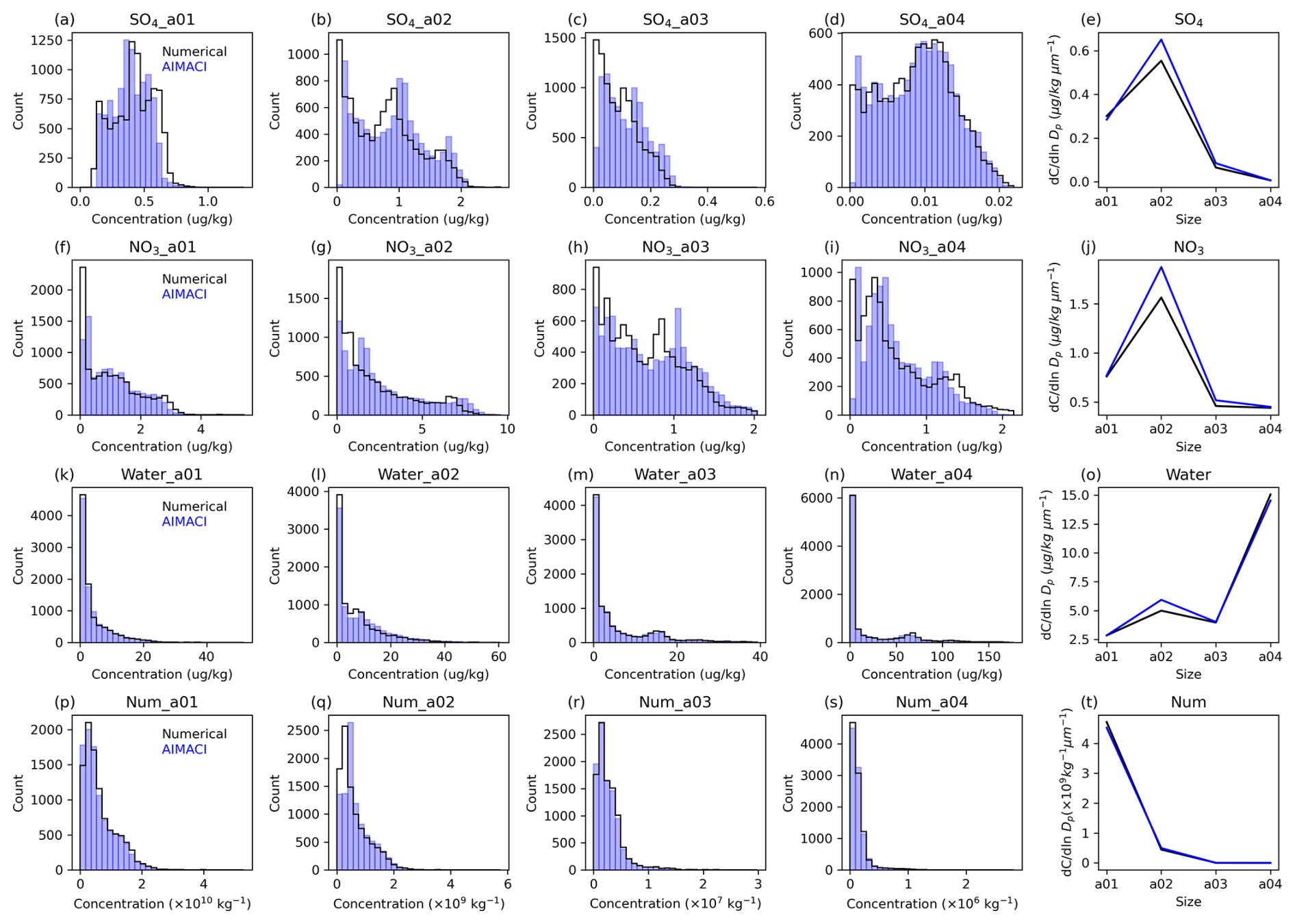
Figure 6 Frequency distributions of different particle sizes for the surface concentrations of four key aerosol species (sulfate (SO4), nitrate (NO₃), liquid water content of aerosol (water), and number concentration of aerosol (Num)), as simulated online by both the numerical scheme and the AIMACI scheme. The last column showcases the particle size distributions of these key aerosol species surface concentrations. The results are calculated by covering the region spanning from 109.1 to 125.9° E and from 22.1 to 44.9° N, with the data being averaged over the entire simulation period.

Figure 5 illustrates the ability of the AIMACI scheme to reproduce temporal variations of surface total concentrations of four key aerosol species. These results represent the calculated averages for the Yangtze River Delta region, a crucial urban agglomeration in China, spanning the coordinates 119.1 to 121.9° E and 30.1 to 31.9° N. Throughout the simulation period, sulfate concentrations primarily fluctuate within the range 0 to 6 µg kg⁻¹, while nitrate concentrations exhibit a broader variability, predominantly ranging from 0 to 20 µg kg⁻¹. Notably, all four key aerosol species experience several instances of abrupt concentration spikes and declines. For instance, between the 11th and 30th hours of the simulation, the liquid water content of aerosol experiences a dramatic increase from 32.86 to 263.47 µg kg⁻¹, followed by a sharp decrease to 28.72 µg kg⁻¹. The occurrence of these pronounced fluctuations may be related to the following factors:

1. Variations in meteorological conditions, such as changes in wind speed and direction, can significantly influence the dispersion and transport of aerosols. Increased wind speed or frequent shifts in wind direction may lead to more pronounced concentration fluctuations. Additionally, changes in humidity can affect the wet scavenging and hygroscopic growth of aerosols. Precipitation events, in particular, can enhance the wet scavenging effect, leading to a significant reduction in aerosol concentrations.

2. Variations in anthropogenic emissions, such as differences in human activities during weekdays and weekends, can also contribute to changes in aerosol concentrations.

A more detailed analysis would be required to identify the specific causes. Despite these pronounced fluctuations, the AIMACI scheme adeptly reproduces these features without introducing systematic bias, achieving R² values larger than 0.97.

The aforementioned analyses have examined the AIMACI scheme's capability in capturing the spatiotemporal distribution and variation trends of major aerosol species. Here, we further assess the scheme's performance in accurately reproducing the evolution of the aerosol particle size distribution (PSD), given that particle size critically governs aerosol radiative properties and cloud nucleation efficiencies – key determinants of atmospheric energy balance and hydrological cycles. Figure 6 presents the PSD and frequency distribution of the surface concentrations for four key aerosol species. The frequency distributions of sulfate and nitrate surface concentrations exhibit a relatively uniform pattern, whereas the liquid water content and number concentration of aerosols display extreme values, leading to pronounced skewness in their distributions. Additionally, there are significant differences in the PSD among the aerosol species. Sulfate and nitrate concentrations peak within the range 0.156 to 0.625 µm (size bin 2), whereas the liquid water content of aerosols is concentrated in the range 2.5 to 10.0 µm (size bin 4) and the number concentration of aerosols is predominantly found in the range 0.039 to 0.156 µm (size bin 1). These findings underscore the challenge of accurately modeling the evolution of the aerosol PSD. However, the AIMACI scheme accurately captures these distributions, highlighting its capability in characterizing complex nonlinear processes.

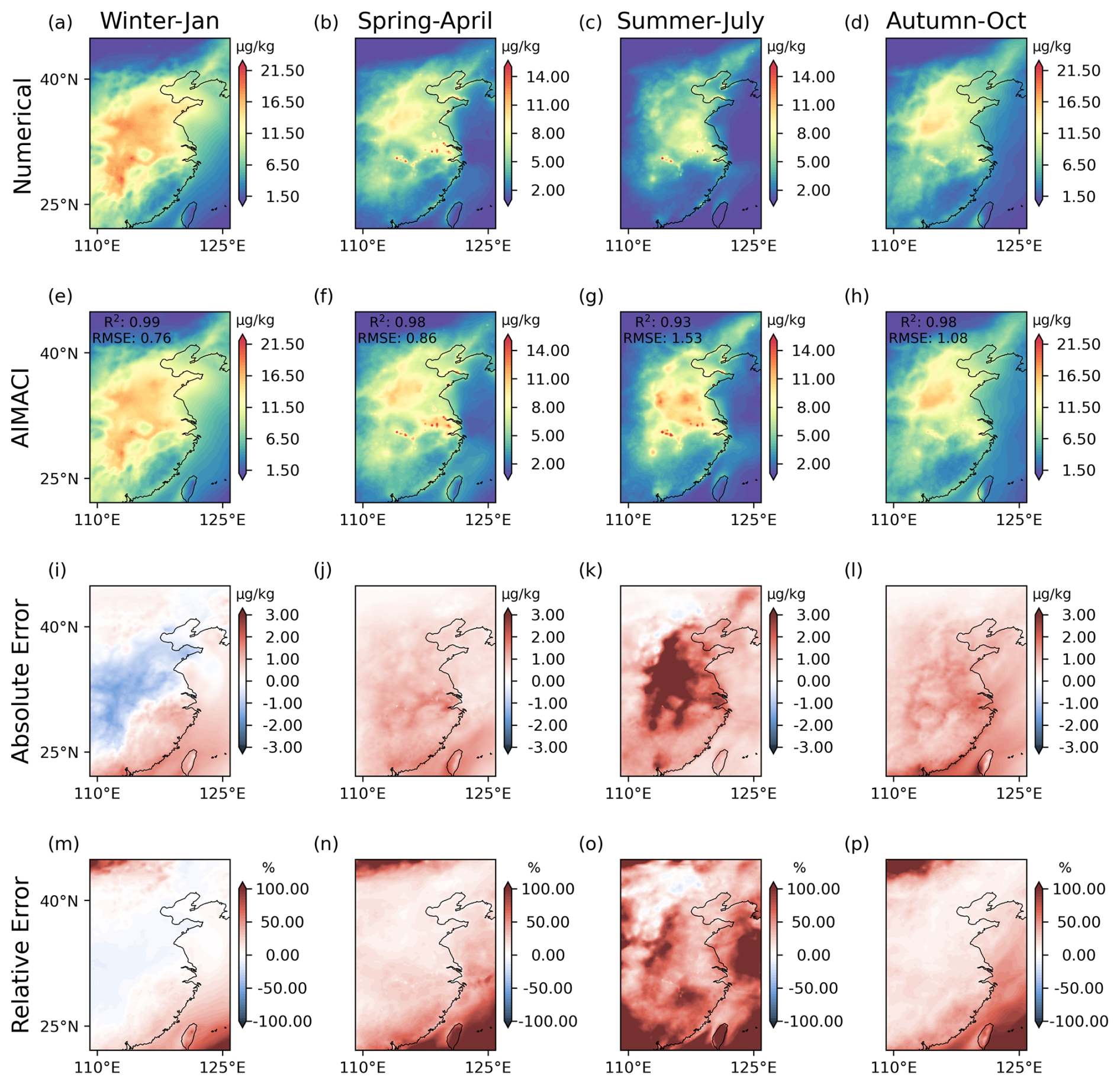
Figure 7 Monthly average surface total concentrations (summed across four size bins) of nitrate for different environmental conditions across seasons, as simulated online by both the numerical scheme and the AIMACI scheme.

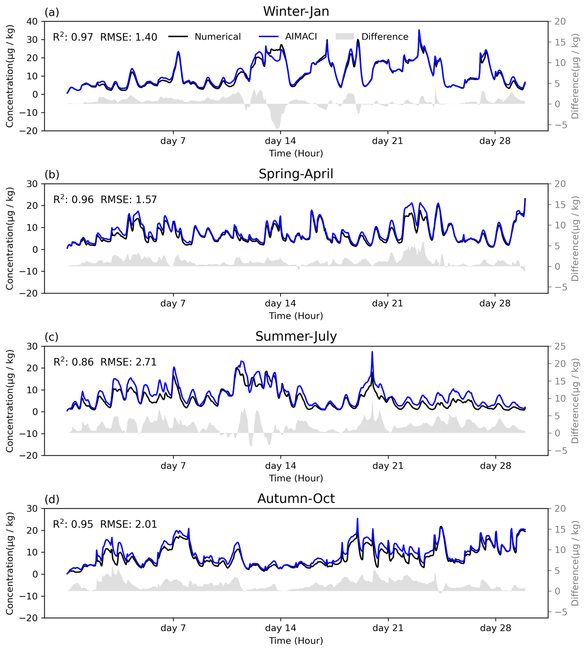
Figure 8 Time series of surface total concentrations (summed across four size bins) of nitrate for different environmental conditions across seasons, as simulated online by both the numerical scheme and the AIMACI scheme. The gray bar is the difference between the two schemes. Results represent the calculated averages for the Yangtze River Delta region (119.1–121.9° E, 30.1–31.9° N).

3.2.2 Robust generalization ability

Following validation of the AIMACI scheme's performance in simulating the 3D spatiotemporal distributions and PSD of major aerosol species concentrations, we assess its generalization ability under diverse environmental conditions, a critical aspect for its future integration into climate models to mitigate uncertainties stemming from oversimplified or absent aerosol processes. To evaluate this, we implemented a comparative analysis of 1 month simulations for each of the four seasons – spring, summer, autumn, and winter – between the numerical scheme and the AIMACI scheme. This comprehensive assessment helps to enhance our understanding of how the AIMACI scheme's performance varies under different meteorological conditions. It also provides insights for future model optimization to improve the stability of long-term simulations.

Figure 7 shows monthly average surface nitrate concentrations simulated by AIMACI across four seasons, with absolute and relative error plots. Nitrate concentrations exhibit seasonal variations, with higher values in January and lower values in July. This pattern corresponds to increased winter heating emissions and enhanced summer atmospheric dispersion from the East Asian monsoon. The spatial distribution of nitrate concentrations shows agreement with the numerical scheme (R² ≥ 0.93), despite AIMACI being trained on only 16 d of March data. Figure 8 displays hourly time series of nitrate concentrations in the Yangtze River Delta (119.1–121.9° E, 30.1–31.9° N). The results reveal that the simulation for January experiences more pronounced concentration fluctuations, with peaks exceeding 30 µg kg⁻¹, while other months' simulations exhibit more rapid concentration variations. Simulating hourly concentration changes poses a greater challenge than simulating multi-day average concentrations, as the latter allows for the offsetting of positive and negative errors. Nonetheless, the AIMACI scheme demonstrates small biases from the numerical scheme (RMSE ≤ 2.71 µg kg⁻¹) and maintains stable performance throughout continuous simulations, with absolute errors oscillating within ±5 µg kg⁻¹ and occasionally approaching zero.

Additionally, we note that the simulation errors in July are notably higher than in other months. Considering that July is a typhoon-prone season, while our training data only include partial data from March, we hypothesize that the lack of representation of such distinct seasonal weather events in our training data may contribute to the larger bias in July. To test this hypothesis, we plotted the minimum values of the mean sea level pressure (MSLP) in the training data and simulation results of different months, as shown in Fig. 9. The time series of the minimum MSLP for different months exhibit some differences from the training data, with July showing the most significant difference. This may be one of the contributing factors leading to the overall suboptimal simulation performance in July. Moreover, we observed the three lowest MSLPs in the time series for April, July, and October, which likely correspond to typhoon events, as indicated by the red points in Fig. 9. Since the lowest MSLP in October is at the start of the simulation, where the concentration of pollutants is almost zero, it may not be diagnostic of simulation bias. Therefore, we additionally selected a relatively later time point, combined with the moments corresponding to the three lowest values, and plotted the spatial distribution of nitrate surface concentrations at these four moments, along with corresponding MSLP and wind fields, as shown in Fig. 10. These results reveal that the lowest values in both July and October correspond to typhoons over the western Pacific, while the lowest value in April corresponds to a low-pressure system over land. The absolute error plot in Fig. 10 shows that, in the regions affected by typhoons, the simulation errors are significantly increased (Fig. 10h, p), whereas the accuracy of the AIMACI scheme in simulating the low-pressure system in April is not significantly impacted. This suggests that, while the AIMACI scheme demonstrates quantifiable generalization capability across diverse environmental conditions, its performance significantly degrades when facing significantly different seasonal weather events, such as typhoons. To surmount these limitations and bolster the precision of the AIMACI scheme, future iterations should consider integrating a more comprehensive and diverse training dataset that accounts for a broader spectrum of environmental conditions, notably incorporating additional seasonal meteorological phenomena, such as typhoons. The augmentation of the training dataset would facilitate the fine-tuning of the AIMACI scheme, thereby enhancing its reliability in delivering robust simulation outcomes.

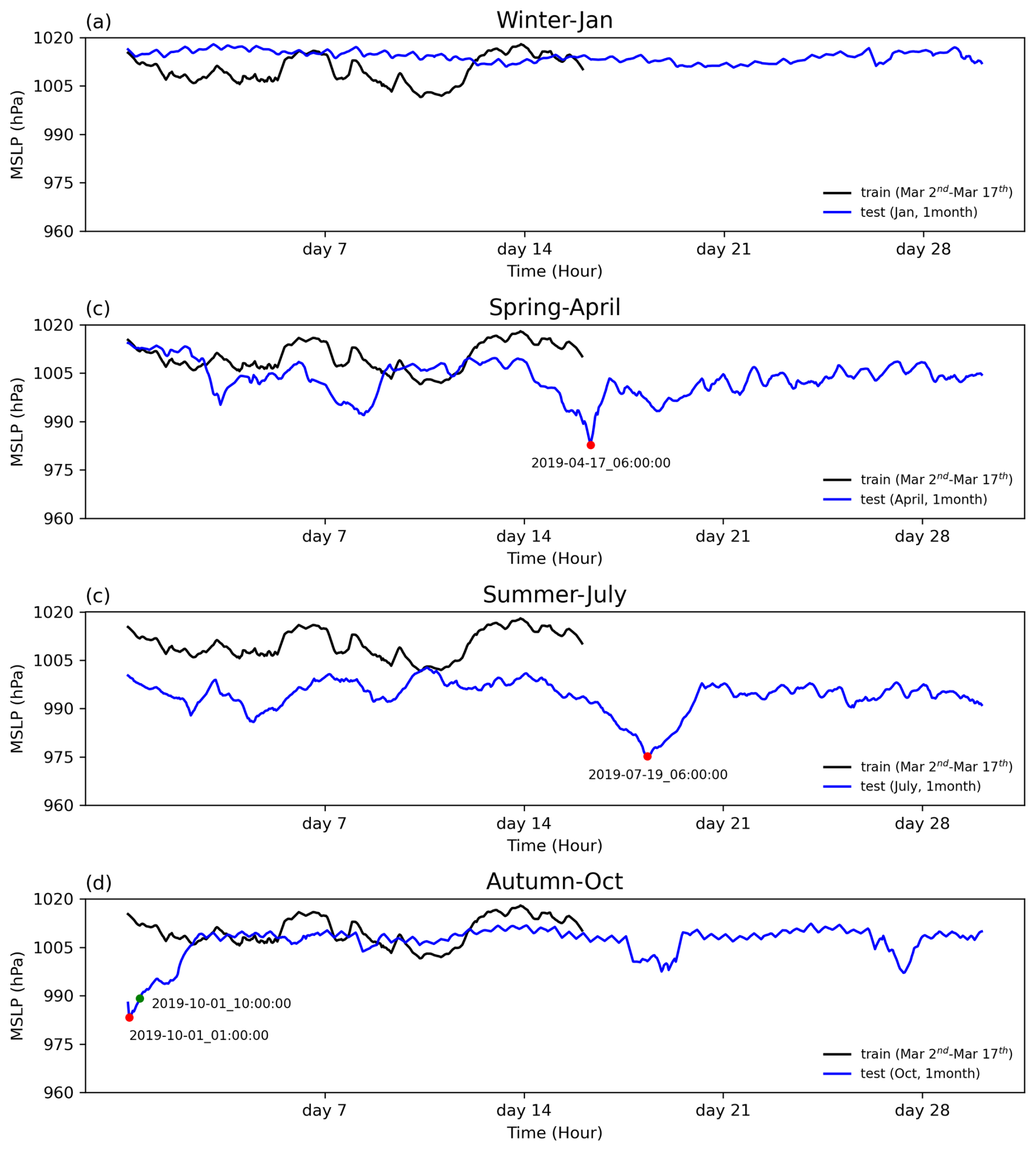
Figure 9 Time series of the minimum of mean sea level pressure (MSLP) in the training data and simulation results of different environmental conditions across seasons. The red points represent the lowest MSLP in the corresponding time series and the date of its occurrence. Since the lowest MSLP in October is at the start of the simulation, where the concentration of pollutants is almost zero, it may not be diagnostic of simulation bias. Therefore, we additionally selected a relatively later time point, as shown by the green point.

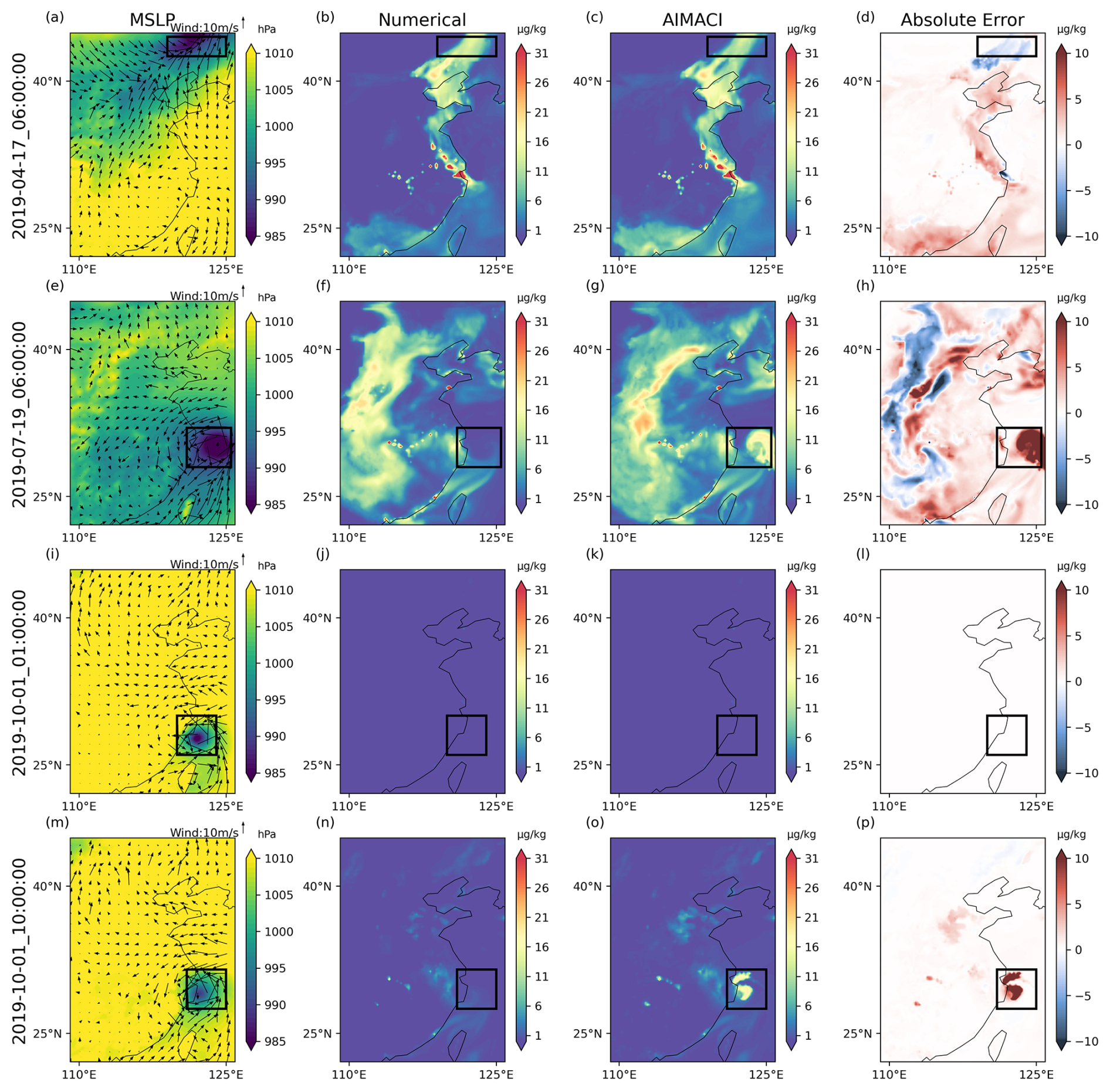
Figure 10 The spatial distribution of nitrate surface concentrations at four specified time points, along with corresponding mean sea level pressure (MSLP) and wind fields. The black box corresponds to the area with the lowest MSLP.

3.2.3 High computational efficiency

A primary motivation for the development of the AIMACI scheme is the potential for increased computational efficiency offered by AI schemes, compared with conventional numerical schemes. However, past research has indicated that such computational efficiency gains are not always guaranteed (Keller and Evans, 2019), necessitating a direct comparison of the computational speeds of the AIMACI scheme and the numerical scheme. Given that WRF-Chem, written in Fortran, is not conducive to GPU acceleration, we conducted offline tests of the AIMACI scheme's computational speed on a GPU and compared it with the numerical scheme on a CPU, where the AIMACI scheme was coupled to the WRF-Chem.

Figure 11 demonstrates that, when utilizing a single CPU core, the AIMACI scheme achieves a computational speedup of approximately 5×, with a time cost of 48.51 s compared with the numerical scheme's 229.74 s. This advancement is further amplified when employing a single GPU: the AIMACI scheme completes the computation in a mere 0.83 s, which is approximately 277× faster than the numerical scheme running on a single CPU core. While it is reasonable to anticipate that future implementation of heterogeneous computing platforms, integrating both CPUs (central processing units) and GPUs (graphics processing units), will yield significant enhancements in computational efficiency, further testing is necessary to account for the potential overhead associated with communication between CPUs and GPUs.

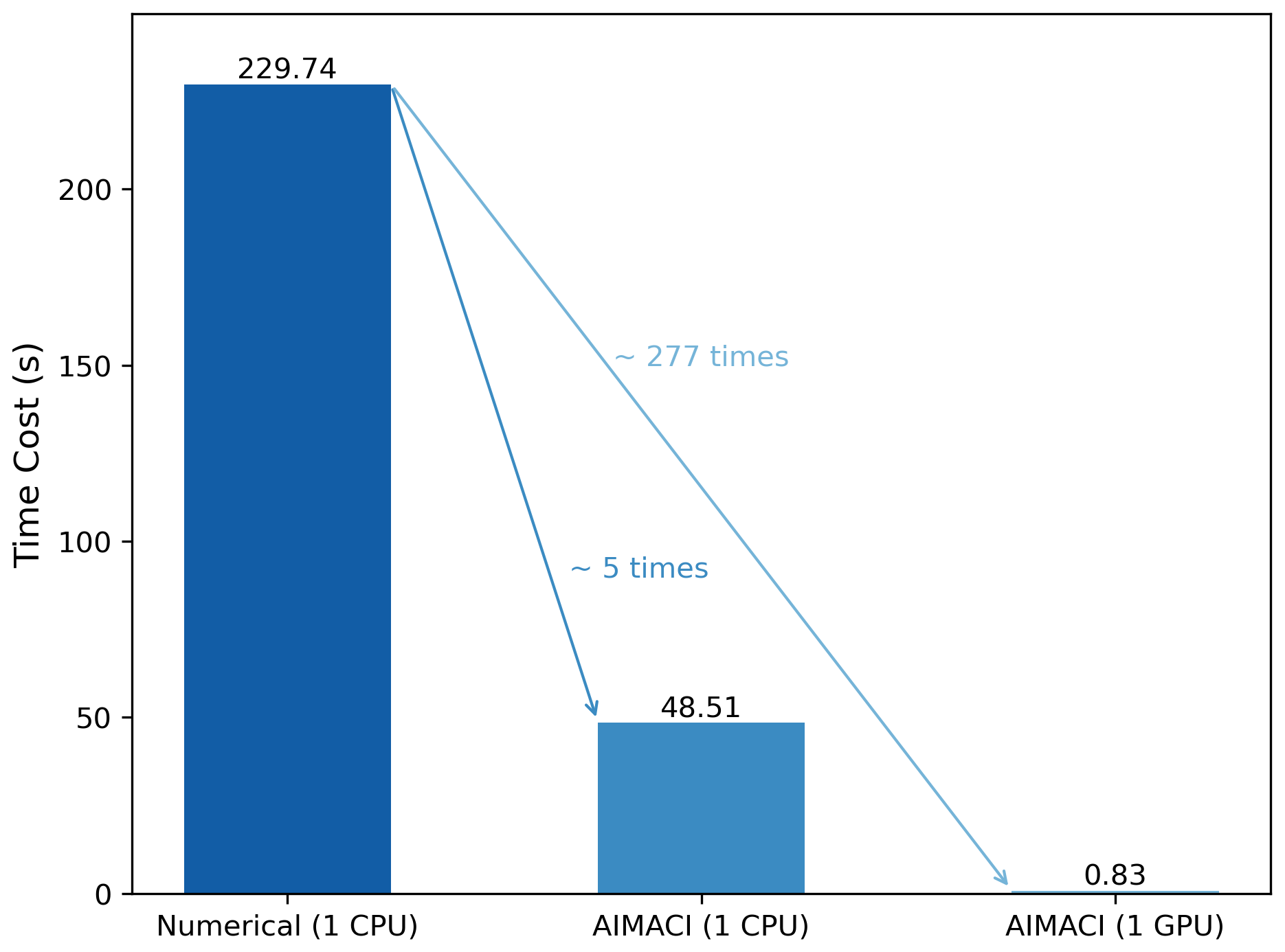
Figure 11 Comparison of computational speeds between the numerical scheme and the AIMACI scheme under different computational configurations. The time cost for the GPU is measured in a mode where the AIMACI scheme is not yet coupled to the model, while the time cost for the CPU is measured in a mode with the AIMACI scheme coupled to the model. The calculations are based on simulating the concentrations of 61 output targets across 720 300 grid cells.

4 Conclusions

This study develops and evaluates a novel Artificial Intelligence Model for Aerosol Chemistry and Interactions, termed AIMACI, with a special focus on addressing the long-standing challenge of significant computational burden caused by using traditional numerical schemes to simulate aerosol chemistry and interactions (ACI) in atmospheric models. The differential equations governing ACI are notably stiff, coupled with a stringent time integration scheme required for numerical stability, resulting in limited breakthroughs in simulation speed with available numerical techniques. While previous studies have explored AI schemes as alternatives for conventional numerical schemes of photochemistry simulation, the application of AI schemes to achieve end-to-end simulation of full ACI within a 3D atmospheric model has not yet been studied. In contrast to atmospheric photochemistry, which only involves chemical reactions among species, full ACI consists of multiple highly nonlinear subprocesses, including chemical reactions and phase equilibrium, gas-particle partitioning, particle size growth, coagulation, and nucleation. Therefore, whether an AI scheme can effectively supplant the traditional numerical scheme for simulating full ACI, achieving both high fidelity in simulation accuracy and a significant improvement in computational efficiency, remains an open question.

To bridge this gap, the AIMACI scheme was established based on the Multi-Head Self-Attention algorithm, which is renowned for its powerful nonlinear representation capabilities and can efficiently capture complex reaction relationships between different chemical species. In an offline mode, where the AIMACI scheme was not yet integrated with a 3D atmospheric model, it demonstrated robust performance on a test dataset, with all 61 evaluated output targets exhibiting an average R² of 0.98, and an average NMB of 3.02 %. This strong consistency between the numerical and AIMACI schemes lays a solid foundation for further online continuous simulations.

To facilitate the coupling of the Python-written AIMACI scheme with Fortran-based numerical models, we utilized PyTorch's TorchScript and LibTorch tools to encapsulate the AIMACI scheme in a static library callable by the numerical model. This approach minimizes changes to the existing numerical model's codebase and offers a lightweight, adaptable, and modular solution for coupling AI algorithms of diverse complexities with a range of numerical models.

Employing a physics-AI hybrid model, we implemented additional experiments to evaluate the online simulation performance of the AIMACI scheme. The 10 d continuous simulation results indicate that the AIMACI scheme not only accurately captures the spatiotemporal distribution of various aerosol species but also effectively reproduces their size distributions, maintaining stability throughout the simulation period without rapid error growth. Furthermore, the AIMACI scheme exhibits robust generalization capabilities despite being trained on data from only 16 d in March. This is evidenced by the results that, during month-long continuous simulations across various environmental conditions in all four seasons, R² for monthly average surface nitrate concentrations is greater than 0.93, and the RMSE for hourly time series of nitrate concentrations in the Yangtze River Delta is smaller than 2.71 µg kg⁻¹. However, systematic biases were observed in the simulation results of the AIMACI scheme: underestimation of high concentrations and overestimation of low concentrations. This bias pattern could be attributed to two main factors. First, the limited number of high-value samples in the training set leads to insufficient learning of high-value instances by the AIMACI scheme. Second, the quadratic term in the RMSE loss function penalizes large errors more heavily, thereby biasing the AIMACI scheme toward predicting the mean of the target distribution to minimize the overall loss. Future improvements may involve exploring data transformation techniques to reduce the skewness of the training data distribution. Additionally, compared with other months, the performance of the AIMACI scheme in July was less accurate. Our analysis indicates that this is primarily due to the significant difference between the meteorological conditions in July and those in the training data. Seasonal weather events, such as typhoons, have a notable impact on the performance of AIMACI. Therefore, in future iterations of AIMACI, we plan to use a more diverse training dataset, particularly one that includes seasonal weather events, to further enhance its performance.

In terms of computational speed, the AIMACI scheme is approximately 5 times faster than the conventional numerical scheme when predicting 720 300 grid points with 61 output targets using a single CPU core. This speedup increases significantly to about 277 times faster when utilizing a GPU. Future simulations on heterogeneous platforms, integrating both CPUs and GPUs, are expected to significantly improve this speedup ratio. However, considering the potential communication overhead between CPUs and GPUs, further testing is still required.

An important outcome of this work is the first-time successful application of an AI scheme to achieve fast, accurate, and stable end-to-end simulation for full ACI within the numerical model, replacing the traditional numerical scheme. As the first step, we mainly focus on inorganic aerosol species and regional-scale monthly simulation tests. Future work will consider integrating complex secondary organic aerosols in our AIMACI scheme, performing global-scale annual simulation tests, and coupling the AIMACI scheme to climate models. These advancements will help to address current limitations in climate models where full ACI is often oversimplified or even omitted due to the large computational burden associated with numerical simulations of ACI, thereby improving the representation of aerosol–climate interactions.