Measurement report: A complex street-level air quality observation campaign in a heavy-traffic area utilizing the multivariate adaptive regression splines method for field calibration of low-cost sensors

As part of the TURBAN project, the “Legerova campaign” investigated air quality and meteorology in a traffic-dense area of Prague, Czech Republic, from 30 May 2022 to 28 March 2023. The study deployed a network of 20 low-cost sensor (LCS) stations to measure NO₂, O₃, PM₁₀ and PM_2.5 concentrations, complemented by advanced meteorological instruments such as a microwave radiometer and Doppler lidar. Ensuring data quality from LCS measurements presented significant challenges. Initial field tests at a reference monitoring station revealed strong correlations between raw LCS and reference data (r > 0.90 for NO₂ and PM_2.5, r > 0.80 for O₃ and PM₁₀). However, individual biases were observed. Applying the multivariate adaptive regression splines (MARS) method effectively reduced biases and enhanced alignment with reference measurements for all pollutants (R² 0.88–0.97). During the campaign, sensor ageing and technical issues were identified through double mass curve analysis and final field testing. The highest NO₂ concentrations were recorded in streets with dense building blocks and traffic lights, corresponding to peak traffic patterns (with medians of concentrations 20–34 ppb). Aerosol concentrations were generally low (medians of PM₁₀ < 25 µg m⁻³ at all sites), with less temporal and spatial variability than NO₂. Elevated PM₁₀ and PM_2.5 levels occurred primarily during temperature inversions, often linked to local sources, and during a short, non-local episode. This study highlights the MARS method as a reliable tool for field calibration of LCS networks and provides valuable data on urban air quality and its dynamics with high spatiotemporal resolution.

1 Introduction

With growing awareness of people around the world of ongoing climate change and the development of appropriate adaptation measures, the need to improve the modelling capabilities of meteorological and air quality conditions in the complex environment of large cities is increasing worldwide. To enable the improvement of atmospheric assessment and advanced modelling in cities, it is always necessary to improve the spatial availability of measured or otherwise estimated data (i.e. indicative measurement, remote sensing monitoring, estimates from satellite data) that may be used for analyses. Since reference meteorological and air quality monitoring (AQM) stations are technically demanding and often not possible to relocate easily for targeted short-term observation campaigns, supplementary non-referential measurements such as low-cost sensors (further abbreviated as LCSs) have become very popular in the last few years (Castell et al., 2017; Kumar et al., 2015; Morawska et al., 2018; Narayana et al., 2022).

Together with better availability, interest in LCSs among laypeople and the interested public and even among scientists has increased (Jerrett et al., 2017; Mahajan et al., 2020; Wesseling et al., 2019). However, their common problem is data quality and how to verify and correct it. Most of the LCSs for ambient AQM are burdened by unstable measurement performance over time and lowered inter-unit precision (Narayana et al., 2022; Peltier et al., 2020). Electrochemical (EC) LCSs for gaseous pollutants are known for their reduced operational lifetime (between 12–15 months on average due to the degradation of electrolyte performance over time); vulnerability to cross-sensitivity of different gases (e.g. known interference between NO₂ and O₃; Baron and Saffell, 2017; Bauerová et al., 2020; Cui et al., 2021; Spinelle et al., 2015); and changes in meteorological conditions, especially air temperature and relative humidity (Bauerová et al., 2020; Collier-Oxandale et al., 2020; Jiao et al., 2016; Mead et al., 2013; Vajs et al., 2021). By contrast, aerosol LCSs based on optical particle counters (OPCs) have a longer operational lifetime (typically 2–3 years) and usually higher inter-unit precision than EC LCSs (Sayahi et al., 2019; Tagle et al., 2020). However, even OPCs are known to interfere with meteorological conditions, especially with relative humidity and air temperature (high probability of measurement error under condensation conditions). The mass concentration of the coarse fraction of aerosol particles (PM₁₀) is usually burdened by weaker measurement performance and by the greater probability of measurement error with respect to relative humidity than the fine fraction PM_2.5 (Bauerová et al., 2020; Crilley et al., 2018; Tagle et al., 2020; Tryner et al., 2020). However, it is known that the error rate of the mass concentrations of all aerosol fractions depends mainly on the type of particle compounds and their ability to bind water (Charron, 2004; Giordano et al., 2021; Robinson et al., 2023; Venkatraman Jagatha et al., 2021; Wang et al., 2021).

A general recommendation to overcome the given uncertainties and drifts of “zero values” in LCS measurement is to undergo the following control process: (1) physical calibration of all the LCSs in a laboratory under controlled conditions; (2) comparative measurement of all LCSs with appropriate reference monitors (RMs) or other equivalent monitors (further abbreviated as EMs) at the AQM station (often called LCS field calibration), followed by the application of a suitable statistical correction method (Clements et al., 2022; Peltier et al., 2020; Schneider et al., 2019; Spinelle et al., 2015); and (3) periodic check of the sensors' performance over time, if possible repeating comparative measurement at the reference station (identification of data drifts). Performing an individual laboratory calibration of a large number of LCSs is relatively technically, financially and time-consuming for most end users (see, for example, Cui et al., 2021, or the European standard CEN/TS 17660-1:2021 (E), 2021, for air quality of LCSs for gaseous pollutants). The advantage of laboratory calibration is the possibility to identify possible differences in sensor response to different concentration levels. On the other hand, it is known that the laboratory calibration alone is not fully sufficient for successful LCS field deployment, as changes in weather conditions and mixtures of gases and compounds occurring in the outdoor environment cannot be demonstrated under controlled conditions (De Vito et al., 2009; Kamionka et al., 2006). Therefore, some studies have already focused fully on field calibration for the evaluation of LCS performance (e.g. Cordero et al., 2018; deSouza et al., 2022; Feinberg et al., 2018; Liu et al., 2020; Mukherjee et al., 2017), as we did in this study. The recommended minimum duration of such a field comparative measurement is 30 to 40 d (CEN/TS 17660-1:2021 (E), 2021; Clements et al., 2022; Peltier et al., 2020; Yatkin et al., 2022a, b). Nevertheless, considering the duration of one season in central European conditions, this length does not ensure that a sufficiently wide range of meteorological conditions would be covered. Therefore, it is even more reasonable to choose a longer period than generally recommended or repeat the field comparison tests after the season changes. Besides this, there are two main challenges of long-term field LCS tests, namely random data drifts and the possibility of performance changes after transfer to another location (De Vito et al., 2009; Papaconstantinou et al., 2023; Sayahi et al., 2019; van Zoest et al., 2019). Therefore, the most common approach follows the general recommendation to collocate at least one sensor at the nearest RM station during the entire final deployment (CEN/TS 17660-1:2021 (E), 2021; Clements et al., 2022; Peltier et al., 2020; Yatkin et al., 2022a, b).

To obtain the most reliable data from the LCS measurements, it is always necessary to find an appropriate technique for statistical correction of raw measured data. Due to the weaknesses of the LCSs described above, it is evident that corrections based on single variable linear regression (i.e. on the relationship between LCSs and RM- or EM-measured concentrations) may not be fully sufficient. Therefore, multiple linear regression (MLR) analyses, generalized additive models (GAMs), random forests (RFs), K-nearest neighbours (KNNs), gradient boosting (GB) and artificial neural networks (ANNs), as well as other complex algorithms that account for additional explanatory variables and non-linear relationships, are increasingly used, achieving different levels of final LCS data quality (Considine et al., 2021; deSouza et al., 2022; Kumar and Sahu, 2021; Mahajan et al., 2020; Narayana et al., 2022). In any case, the applied correction method should be sufficiently transparent and computationally reproducible (avoiding black box methods), which is not always true for some new statistical machine learning techniques (e.g. random forests, neural networks). From this point of view, the multivariate adaptive regression splines (MARS) method can be a suitable statistical tool for LCS measurement correction since it is a non-parametric regression technique that can reflect non-linearities and different interactions between several continuous or categorical data (Friedman, 1991a, b). Generally, the MARS method is flexible and simple to understand and interpret and requires almost no data preprocessing (is capable of dealing with “noisy” data). Moreover, it is computationally time-feasible and reproducible (Friedman, 1991a, b; García Nieto and Álvarez Antón, 2014; Keshtegar et al., 2018; Everingham et al., 2011). When using MARS, the exact form of the non-linearity does not need to be known explicitly or determined a priori. The algorithm will search for, and detect, non-linearities in the data that help maximize the performance of LCSs' data correction procedure. In addition, if the algorithm is sufficiently trained (during field comparative measurement), data from the RM are no longer needed to calculate the corrected concentration values.

A common challenge when using different machine learning techniques is the possible loss of accuracy due to the incompleteness of the initially defined computation model, leading to “concept drift” (De Vito et al., 2020; Ditzler et al., 2015). Therefore, it is still recommended to perform continuous or backward controls of the performance of any correction algorithm used (similar to the previously mentioned need for LCS data drift control). Several data control mechanisms have already been described in papers focusing on LCS measurement (De Vito et al., 2020; Harkat et al., 2018). However, to our knowledge, no previous study has used the double mass curve (DMC) method for data continuity control in LCS measurement. The DMC is a simple graphic method usually used for checking the consistency of hydrological and climatological data continuously measured at several stations in a selected area (Kliment et al., 2011; Liu et al., 2023). Based on our experience, we assume that it is fully applicable to control the performance of the LCS network measurement.

For the possibility of a better understanding of complex atmospheric processes in the urban environment (including the accumulation and dispersion of pollutants), it is important to obtain data from different heights, not only within the urban canopy layer but also above it. Therefore the combination of traditional ground measurement with remote sensing monitoring of temperature and wind profiles above the rooftops is beneficial (Allwine et al., 2002; de Arruda Moreira et al., 2020, 2018; Münkel et al., 2007). The advantage of using microwave radiometers (MWRs for temperature profiles) and Doppler light detection and ranging systems (lidars for wind profiles) nowadays is their high temporal resolution (compared to radiosondes), portability and the possibility of installation in the city without disturbing the surroundings (in contrast to acoustic wind profilers or SODAR-RASS systems; Lokoshchenko et al., 2009; Tamura et al., 2001). However, even these devices are burdened by their technical limitations, and some data verification is recommended (if not against the available RM, at least compared to other remote sensing measurements). The Doppler lidars' accuracy of wind measurement can be deteriorated by rain (and low stratus clouds), and profiles have a high vertical resolution but non-stable height range because of the varying signal-to-noise ratio (SNR). The MWRs' measurement performance is quite independent of meteorological conditions (with some exceptions in older instruments as in Ezau et al., 2013); moreover, MWRs have null overlap and do not use aerosols as tracers. On the other hand, MWRs usually have a stable height range but a lower vertical resolution than lidars (de Arruda Moreira et al., 2020, 2018). Both systems were used in the TURBAN measurement campaign to allow monitoring of the boundary layer conditions (temperature and wind vertical profiles) at the target site.

The objective of this study was to obtain credible air quality and meteorological data using a high-spatiotemporal-resolution supplementary network consisting of air quality LCSs, MWRs and Doppler lidars in a part of the city centre of Prague (within Legerova street and its surroundings; Prague 2 district, the Czech Republic) to support the validation of the updated LES PALM microscale model (Patiño et al., 2024; Resler et al., 2024). This area represents a typical urban environment with a high traffic load within central European cities. The Prague Legerova reference AQM station is classified as a hotspot (see NO, NO₂ and NO_x measurement statistics across all traffic stations in Prague in Table S1 in the Supplement). Therefore, it is also one of the most frequent target locations for public attention and protest actions to limit automotive traffic (and automotive speed) in Prague. Innovative procedures resolving the quality of the LCSs' data were applied in this study: long-term field testing of all LCSs was performed before their target deployment, the MARS statistical method was used for correction of the original LCSs' data and possible data drifts were identified using the DMC method. The paper is structured according to its main objectives: (1) evaluation of LCS data quality and performance of MARS correction method used in the TURBAN project, (2) monitoring of raw and corrected data quality during the Legerova campaign and after the end of the project, and (3) analysis of air quality measurement results during the Prague Legerova campaign including interesting episodes related to meteorological conditions in the atmospheric boundary layer.

2 Materials and methods

2.1 Study area and experimental design

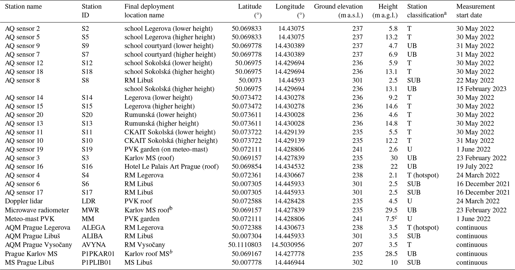
The study area of the TURBAN measurement campaign covered the streets of Legerova, Sokolská and Rumunská and their immediate surroundings (district of Prague 2, Czech Republic; Fig. 1) including the urban traffic hotspot AQM station of Czech Hydrometeorological Institute (CHMI) called “Prague Legerova” (locality code: ALEGA; CHMI, 2025a) and the adjacent “Prague Karlov” professional meteorological station (MS) placed on a building roof (station ID: P1PKAR01; WMO, 2023a). Legerova, Rumunská and Sokolská streets are characterized by a high daily traffic load (the traffic intensity is between 35 000 and 45 000 cars per day; TSK, 2023) and street canyon conditions consisting mainly of compact midrise buildings on both sides of the streets (with only small fractions of open spaces). Particularly problematic in the long term are the high concentrations of NO₂, which, despite improvements in recent years, still reach the applicable limit value (see Figs. S1–S3 in the Supplement). For the TURBAN measurement campaign (further referred to as the Legerova campaign), a total of 20 combined LCS stations (for NO₂, O₃, PM₁₀ and PM_2.5) have been deployed in this area and measured mainly from 30 May 2022 to March 2023 (except for the LCSs S3, S4 and S16; see details in Table 1). Of these, 11 LCSs were placed in the streets with the highest traffic load: 10 LCSs were installed in pairs at two different height levels (first 5–7 m a.g.l. and second 12–15 m a.g.l.) in five locations, and 1 LCS (identified as S4) was collocated with the Prague 2-Legerova traffic AQM station throughout the entire campaign. Furthermore, five LCSs were installed at greater distances and higher heights from these streets and were established as background locations: two LCSs on the roofs of the Prague Karlov MS (S3; 30 m a.g.l.) and Le Palais Art Hotel Prague (S16; 22 m a.g.l.), two LCSs (S7 and S9; 5 and 7 m a.g.l.) within the closed school courtyard (a student sports field with no traffic), and one LCS (S19; 3 m a.g.l.) at a mobile meteorological mast installed about 50 m away from the middle of Sokolská street (see Fig. S4 in the Supplement). Examples of photos from the LCS installation are shown in Fig. 2. The meteorological mast (hereinafter abbreviated as MM) was deployed in the garden of the Prague Waterworks and Sewerage Company (hereinafter referred to as the PVK garden) for basic meteorological measurement below the level of the rooftop in this area. Furthermore, one Doppler lidar (for wind vertical profile) was installed on the roof of the PVK administrative building (hereinafter referred to as the PVK roof), and one MWR (for temperature vertical profile) was installed on the roof of the Prague Karlov (for both see Fig. S4 in the Supplement). A complete list of measurements, installation sites and other metadata is given in Table 1 and shown in Fig. 1c.

The performance of all LCSs was tested before and after the end of the Legerova campaign at the Prague Libuš suburban background AQM station (locality code: ALIBA; CHMI, 2025b; Fig. 3) with the adjacent Prague Libuš professional MS (station ID: P1PLIB01; WMO, 2023b), both located outside of the Legerova target domain (see station position in Fig. 1b). The initial field comparative measurement lasted for most of the LCS stations (17 out of 20) from 16 December 2021 until 30 May 2022 (165 d). During this time, three LCSs were identified as defective (two were replaced later), the settings of all LCSs were synchronized (device time and data transfer to the data storage server), and measurement deviations and errors were identified against the appropriate RMs (gases) and EM (aerosols). In two exceptions, the initial field comparative measurement lasted for a shorter period, namely until 23 February 2022 for LCS S3 (69 d) and until 24 March 2022 for LCS S4 (98 d) due to the earlier installation of these sensors to target locations, namely at the Prague Karlov MS roof (LCS S3) and at the Prague Legerova AQM station (S4). Two sensors (S8 and S17) identified as faulty during the initial field comparative measurement were later replaced, compared on separate dates and left together with LCS S6 at the Prague Libuš AQM station; they later served as verified spare units in the case of failure of other sensors. After the end of the Legerova campaign, a final comparative measurement of all LCSs was done (lasting from 9 May to 14 June 2023, i.e. 37 d) to re-assess the data quality (both raw and corrected). All data gained during comparative measurements were used for the statistical data correction process described in Sect. 2.3.

Table 1 List of all measuring instruments used with the metadata for specific deployment sites during the Legerova campaign. Coordinates are given in decimal degrees. Station classification follows the classification method used in the air quality (AQ) reference monitoring network (CHMI, Czech Republic).

^a T is urban traffic, UB is the urban background, SUB is the suburban background and U is urban. ^b Prague Karlov MS is placed on the top of the building roof at 29.5 m a.g.l. ^c The height of wind measurement at the top of the meteorological mast.

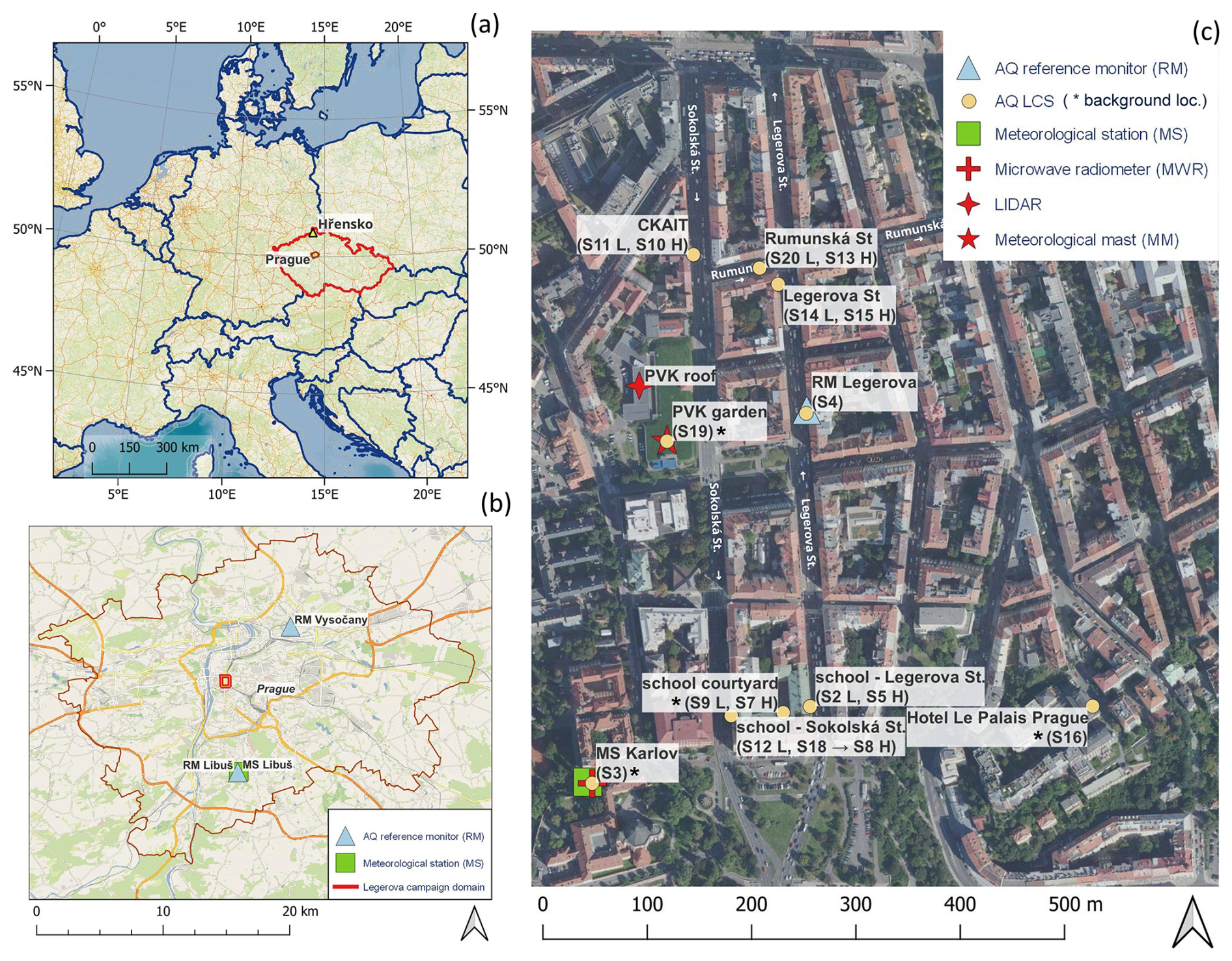
Figure 1 (a) Map of the Czech Republic with the city of Prague and the locality of Hřensko highlighted. (b) Map of the city of Prague with Legerova location selected (highlighted in red rectangle), Libuš reference monitoring station and meteorological station, and Vysočany reference monitoring station. (c) Map of the individual device placement within the Legerova campaign. Sx is the individual low-cost sensors for air quality monitoring (AQ LCS), L is the lower height (m a.g.l.) and H is the higher height (m a.g.l.). Background sites are marked with an asterisk. State boundaries in (a) © EuroGeographics. Background data in (a) and (b) are an Open Street Map provided by WMS by Terrestris GmbH & Co. KG. Orthophoto in (c) is provided through WMS by the Czech Office for Surveying, Mapping and Cadastre – ČÚZK.

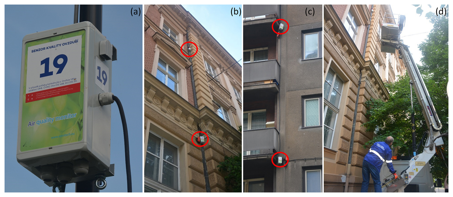
Figure 2 Photos of LCSs deployed in the Legerova campaign (Prague, Czech Republic). (a) The detailed picture of LCS stations used for monitoring of NO₂, O₃, PM₁₀ and PM_2.5 concentrations. (b, c) Installation of LCSs at two different height levels at the Sokolská school location and Legerova location. (d) Picture of the lift platform used for installation of LCSs.

Figure 3 (a) Initial field comparative measurement of all LCSs (for measuring NO₂, O₃, PM₁₀ and PM_2.5) conducted at the Prague Libuš AQM station (CHMI, 2025b) from 21 December 2021 to 30 May 2022. (b) LCS stations in detail.

2.2 Technical specification of instruments used and measurement methods

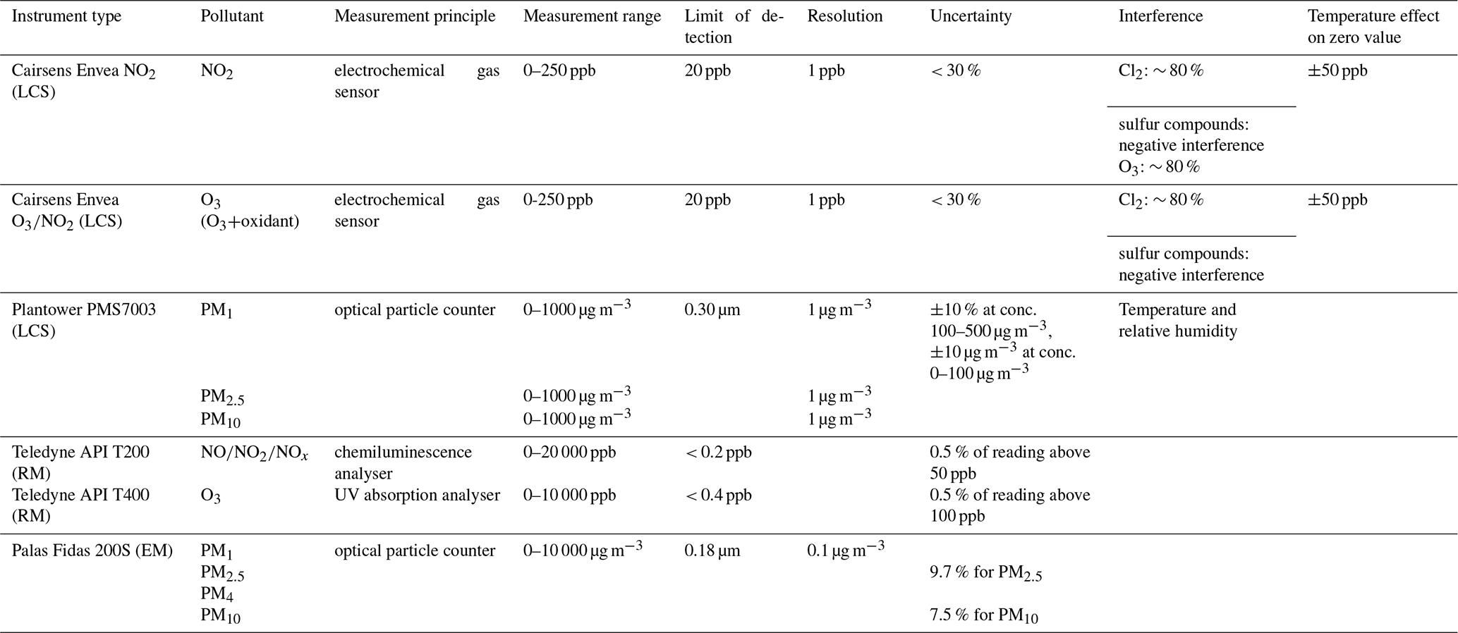
For the air quality monitoring, 20 combined LCS enviSENS platforms (Envitech Bohemia, CZ) were used. They were constructed as small airflow boxes with dimensions of $\mathrm{125}\times \mathrm{225}\times \mathrm{110}$ mm, each equipped with a Cairsense EC LCS for NO₂ and O₃ (combined ${\mathrm{O}}_{\mathrm{3}}/{\mathrm{NO}}_{\mathrm{2}}$ sensor; FR; Envea, 2023) and low-cost aerosol particle counter PMS7003 (CN; Plantower, 2023) for PM₁₀ and PM_2.5 mass concentrations (see Table 2 for the main technical parameters). This selection was based on our previous experience with an almost 1-year testing field comparative measurement (Bauerová et al., 2020). All LCS stations were powered by 230 V electricity, and the data were transferred remotely via LTE modems to the internal server of CHMI. The measurement frequency was set to 10 min intervals in all sensors, from which 1 h averages were calculated. Furthermore, the data from RMs and EMs measuring at AQM stations Prague Legerova and Prague Libuš were used as a control. All AQM stations are equipped with the RM Teledyne API T200 for NO₂ monitoring based on the chemiluminescence detection principle, RM Teledyne API T400 for O₃ monitoring based on UV absorption (US; Teledyne API, 2023a, b), and EM Palas Fidas 200 S (DE; Palas, 2023) optical particle counters for the measurement of PM₁₀ and PM_2.5. Since the RM for O₃ measurement is not available at the Prague Legerova urban traffic station, as a substitute, O₃ concentrations measured at the Prague Vysočany AQM station (classified as an urban traffic station; CHMI, 2025c; see station position in Fig. 1b) were used for indicative comparison with O₃ LCS measurement during the Legerova campaign. The technical parameters of all used devices are listed in Table 2.

Technical specifications and measurement methods of ground-based and remote sensing meteorological instruments used within the Legerova campaign are described in Sect. S2.2 in the Supplement.

Table 2 Technical parameters of LCSs and reference and equivalent monitors (RMs and EMs) were used in this study. Source of parameters: Envea (2023), Palas (2023), Plantower (2023) and Teledyne API (2023a, b).

2.3 Data processing and statistical analyses

A summary diagram of the entire LCS air quality data control process with correction methods used and the evaluation of the correction performance is shown in Fig. 4.

In the first step, the data from the initial field comparative measurement of all LCSs were processed. Raw measured concentrations underwent quality checks before calculating 1 h averages; i.e. hours with more than 30 % missing samples (due to instrument defects, power outages, etc.) were marked as not available (NA) and were omitted from further processing. Then summary statistics for the checked data (1 h LCSs', RMs' or EMs' concentrations) were calculated and visualized using R software (R Core Team, 2021) with the following packages: ggplot2 for box plots (Wickham, 2016), corrplot for correlation matrices (Wei and Simko, 2021), openair for time–variation graphs (Carslaw and Ropkins, 2019), tdr for statistical error calculation (Lamigueiro, 2022) and plotrix for the Taylor diagram visualization (Lemon, 2006). Summary statistics included the coefficient of variation (CV) to express mean precision of LCS measurements during field measurements, along with mean, median, standard deviation (SD) and parameters derived from regression analyses: intercept (a), slope (b), coefficient of determination (R²), Williamson–York regression parameters (a, b, using the maximum given RM, EM and LCS uncertainties; according to Cantrell, 2008), mean bias error (MBE) and root mean square error (RMSE). No significant outliers, defined as values greater than 3 times the maximum of the hourly average concentration measured by an RM or EM (Bauerová et al., 2020; van Zoest et al., 2018), were detected during the testing period (not even during the Legerova campaign or during the final comparative measurement). Therefore, all LCS raw measured data were used in the subsequent statistical correction process.

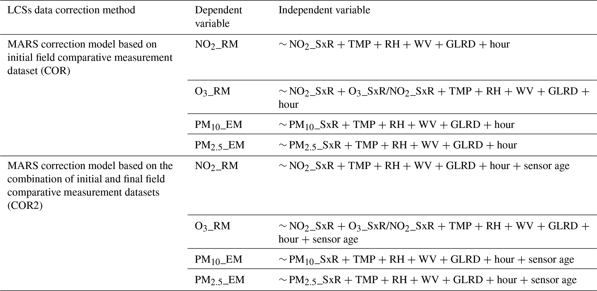
In the second step, the raw LCS data were corrected using the MARS statistical method (Friedman, 1991b; Everingham et al., 2011; see Sect. S2.3.1 in the Supplement for detailed description of this computational method). Software options for MARS analysis include the free R package earth (Milborrow, 2011) or commercial products such as TIBCO Statistica (version 13.1.0; TIBCO, 2020), which were used in this study. The main correction equations (COR) were calculated for each LCS separately based on the dataset gained during the initial field comparative measurement. All MARS correction equations were built of 1 h concentrations measured by an RM or EM as a dependent variable and the following list of continuous independent/explanatory variables: 1 h concentrations measured by LCS, further 1 h averaged temperature (TMP), relative humidity (RH), wind velocity (WV), global radiation intensity (GLRD) and hour of the day. The maximum number of basis functions in the MARS equation was set to 21, the degree of interactions to 1 (i.e. no interactions included), the penalty to 2 and the threshold to 0.0005 (and pruning was allowed). In the case of O₃ measurement, besides the raw O₃ concentration, the ratio of ${\mathrm{O}}_{\mathrm{3}}/{\mathrm{NO}}_{\mathrm{2}}$ concentration from separate LCSs was added as explanatory variables (for the possibility of taking into account the interference effect of the combined ${\mathrm{O}}_{\mathrm{3}}/{\mathrm{NO}}_{\mathrm{2}}$ sensor). The summary statistics of MARS correction equation performance for each LCS, including the frequencies of use of each independent variable/predictor, are listed in Tables S2–S9. An example of the calculation of corrected NO₂, O₃, PM₁₀ and PM_2.5 concentrations based on the MARS correction equation (COR) in the case of LCS S2 is shown in Table S10.

Within the framework of testing different correction methods, one alternative method was chosen during the process of finding the optimal correction procedure. This method was named COR2 and was based on MARS correction calculated on the combined dataset from the initial and final comparative measurements at the Prague 4-Libuš station (i.e. combined data gained from 16 December 2021–30 May 2022 and 9 May–14 June 2023). This combined dataset assumes the inclusion of the change in the quality of the raw LCS measurement at the end of the measurement campaign (after more than 1.5 years of sensor measurement in the field). The conditions for calculating the correction were similar to those in the case of the initial correction (COR), with the age of sensors added to independent/explanatory variables. The resulting correction equations (COR and COR2) obtained for individual LCSs were applied to calculate the corrected concentrations of particular LCSs during the Legerova campaign, utilizing meteorological data from the Prague Karlov MS (see overview in Table 3).

In the third step, a double mass curve (DMC) method was used (Searcy and Hardison, 1960) to check data consistency and identify possible random or systematic data drifts in raw LCS concentrations. This method involves linear regression of cumulative 1 h average RM concentrations (independent variable; the abscissa) against cumulative raw and corrected 1 h average LCS concentrations (dependent variable; the ordinate), both over the entire period. Deviations from the linear regression fit indicate a change or break points in LCS measurement (data gaps, abrupt or systematic gradual data drifts, change of measurement location). This method was applied to the entire LCSs' measurement. For the Legerova campaign, all the LCS raw and corrected concentrations were indicatively compared with the concentrations measured by an RM (in the case of NO₂) or EM (in the case of aerosols) at the Prague Legerova AQM station and by a more distant RM at the Prague Vysočany (in the case of O₃).

Further details on the preparation of the meteorological data obtained during the Legerova campaign and their statistical analyses are described in Sect. S2.3.2 in the Supplement.

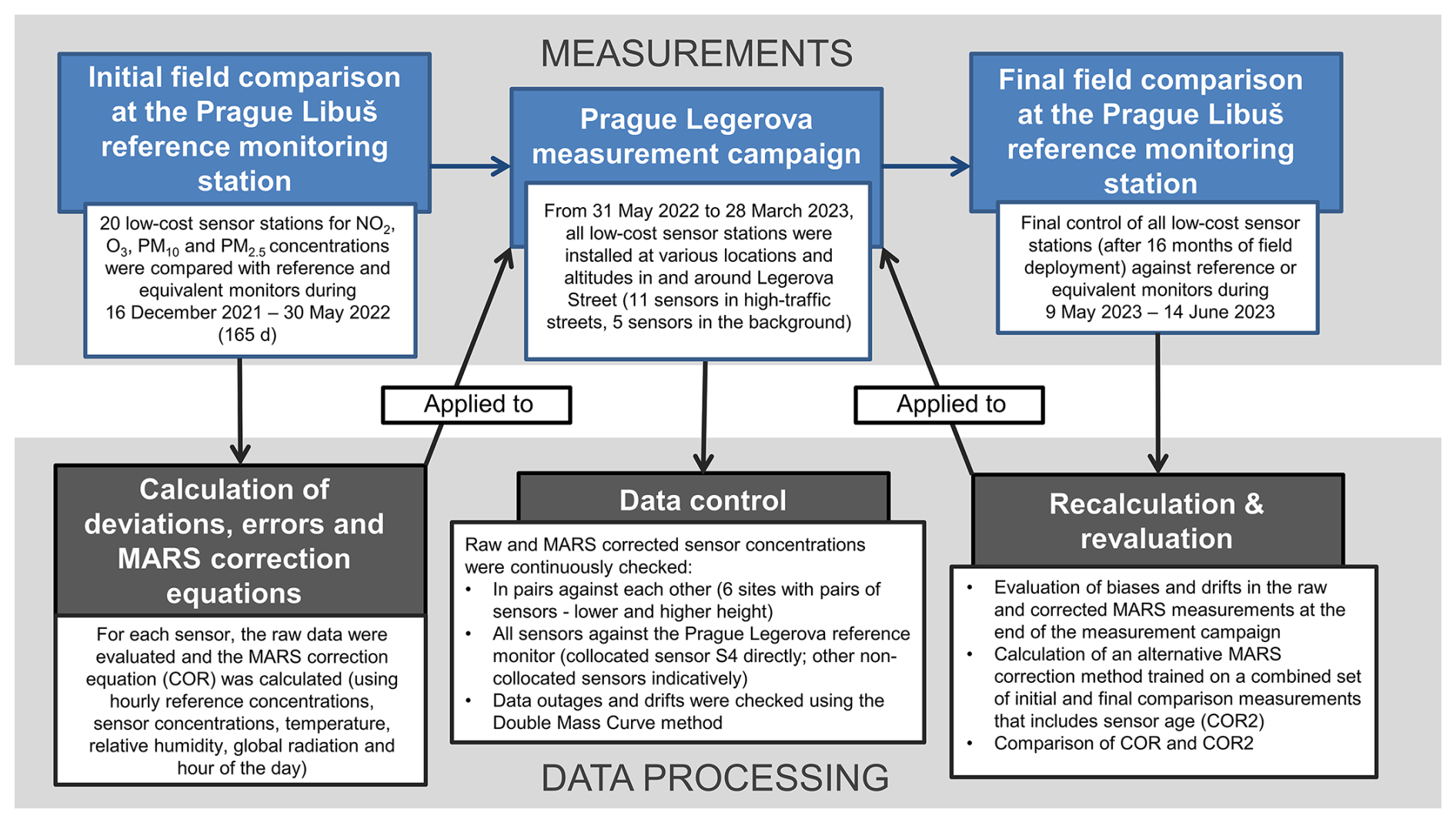
Figure 4 Summary scheme of particular steps in the LCS air quality measurement process, data control, correction methods and evaluation of correction performance.

Table 3 Description of the MARS correction models used to correct the raw sensor data. RM denotes the concentrations from the reference monitor (gases), EM denotes the concentrations from the equivalent monitor (aerosols), SxR denotes the raw measured concentrations from the particular sensor, TMP is the air temperature (in °C), RH is the relative humidity (in %), WV is the wind velocity (in m s⁻¹), GLRD is the solar radiation intensity (W m⁻²), hour is the hour of the day (UTC) and sensor age is the age of the sensor (in days).

3 Results

3.1 Data quality verification – results

The initial field comparative measurement of all the LCSs (17 stations, except 3 broken ones) showed differences/variability between individual LCSs raw measurement and also between each LCS and RM measurement (see standard deviations and correlation coefficients in Fig. 5, box plots in Fig. 6 and a 1-month data example in Fig. S7 in the Supplement). The mean coefficients of variation (CVs) for original (raw) LCS measurements were 27.69 %, 16.71 %, 23.44 % and 23.16 % for NO₂, O₃, PM₁₀ and PM_2.5, respectively; see Table S11 in the Supplement). The comparison with RMs or EMs showed the following correlation coefficients: r>0.90 in all NO₂, PM₁₀ and PM_2.5 LCSs and r>0.80 in all O₃ LCSs (all correlations statistically significant at the level p< 0.001). The results of linear regression showed R² in the range 0.84–0.98 for NO₂, 0.54–0.82 for O₃, 0.72–0.89 for PM₁₀ and 0.85–0.91 for PM_2.5 and slopes 0.63–0.84 for NO₂, 0.30–0.83 for O₃, 0.65–1.72 for PM₁₀ and 0.77–1.51 for PM_2.5. The complete results of the summary statistics of LCS raw measurements, including intercepts (a) and slopes (b) from linear regressions and bivariate regressions and the statistical errors MBE and RMSE, are available in Tables S12–S15 and Figs. S9–S12 in the Supplement.

The MARS correction decreased the differences between LCS concentrations and RM or EM concentrations and between individual LCS measurements (see Figs. 5–6 and S8 in the Supplement). The mean CVs for LCS measurements after correction were 9.25 %, 6.06 %, 13.05 % and 14.62 % for NO₂, O₃, PM_2.5 and PM₁₀, respectively (Table S11 in the Supplement). The corrections also improved the relationship of the LCS data with the data from RMs or EMs: R² in the range 0.89–0.99 for NO₂, 0.91–0.96 for O₃, 0.75–0.92 for PM₁₀ and 0.91–0.95 for PM_2.5 and slopes of 0.89–0.99, 0.91–0.96, 0.83–0.92 and 0.91–0.95, in the order of pollutants as previously. For complete summary statistics, see Tables S12–S15 and Figs. S9–S12 in the Supplement. Three LCSs showed slightly different performance after the application of MARS correction (see Fig. 5), namely LCSs S3, S4 and S11 in the case of NO₂ measurement. The overall improvement of LCSs' measurement after the application of the MARS corrections was also confirmed by the DMC method (see Figs. S13–S14 in the Supplement). However, after correction, some initially very low concentrations turned into weakly negative values: for gaseous pollutants, they constituted less than 0.3 % and for aerosol, less than 2.6 % of the whole testing dataset (part of the summary statistics in Tables S12–S15 in the Supplement).

During the Legerova campaign itself, the concentrations of all monitored pollutants were highly correlated in each LCS pair (i.e. sensors S11+S10, S20+S13, S14+S15, S2+S5, S12+S18, S9+S7 and S4+RM; always mentioned as lower (L) + higher (H) elevation; see Figs. S15–S22 with courses of concentrations and Figs. S23–S24 in Supplement showing particular relationships with the RM Legerova measurement). The only sensor identified as defective during the Legerova campaign was the NO₂ LCS S9 placed within the closed school courtyard, which showed a significant, gradually increasing data drift to high concentrations over time (Fig. S20a in the Supplement). For NO₂, in addition to the LCS, S9, mentioned already, the other LCSs, S11 and S12, were also identified for possible systematic gradual data drift by the DMC method (see Fig. S25 in the Supplement). Some technical issues must have occurred in the O₃ LCSs, where, in all sensor units, a sudden partial data drift occurred from October to November 2022 (see Fig. S26). Therefore, there is no clear warranty in O₃ data after 15 October 2022. In the case of the aerosol LCS measurement (PM₁₀ and PM_2.5), no data drifts were identified based on the DMC method (Fig. S27 in the Supplement).

Last but not least, the ranges and medians of raw and MARS-corrected LCS concentrations of all pollutants during the final comparative measurement at the Prague Libuš AQM station are shown in Fig. S28 in the Supplement. In the case of NO₂ measurement, 10 out of the 17 LCSs achieved R²>0.80 with corrected concentrations (COR); 5 LCSs achieved R²>0.60; LCS S4 achieved R²=0.56; and the weakest relationship was detected in S9, with R²=0.17 (for the complete statistics of all LCSs including statistical errors, slopes and intercepts, see Table S16 and Fig. S29 in the Supplement). The absence of a relationship in the case of LCS S9 during the final comparison confirmed the sensor failure, and therefore this sensor was not used for Legerova campaign evaluation. In the case of O₃, the improvement of the relationship between RM data and the corrected data was not significant at the end of the measurement campaign; in LCSs S3 and S4, the relationships were even slightly worsened (Fig. S28 in the Supplement). Although R²>0.85 was achieved in all O₃ LCSs compared to RM data, the intercept was shifted to negative values (i.e. the corrected concentrations were underestimated at the end of the measurement campaign in most of the O₃ LCSs; for complete statistics, see Table S17 and Fig. S30 in the Supplement). In aerosol measurement, the weakest relationships compared to EM were reached in the case of PM₁₀ concentrations. Although MARS-corrected concentrations significantly improved the relationship with EM and narrowed the variation of originally measured concentrations even at the end of the campaign (Fig. S28 in the Supplement), the R² ranged only from 0.47 to 0.63 (Table S18). The worst relationship was achieved for the S3 LCS, which, even after correction, significantly underestimated the PM₁₀ concentrations compared to the EM (see Fig. S31 in the Supplement). Better relationships were achieved for PM_2.5 measurement, with resulting R² values between 0.73 and 0.89, where none of the LCSs achieved significantly underestimated or overestimated concentrations, even at the end of the campaign (see Table S19 and Fig. S32 in the Supplement). Recalculation of the COR2 correction method (taking into account the initial and final comparison measurements and the LCS age) yielded similar results, with the difference that COR2 sometimes behaved inappropriately at low concentrations (intercept/absolute term ranging between −2.68 and 9.20; see Fig. S33 in the Supplement). Therefore, the COR correction method was used to evaluate the Legerova measurement campaign. Examples of linear regression results of NO₂, O₃ and PM₁₀ concentrations corrected by the COR and COR2 method for LCSs S2, S4 and S6 and the EM are shown in Fig. S34 in the Supplement.

The complete results of meteorological data verification are shown in the Supplement in Sect. S3.1.5.

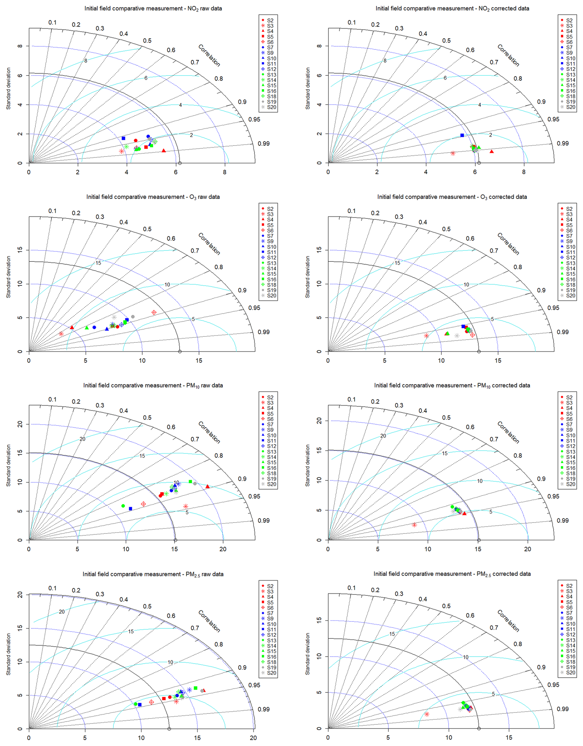
Figure 5 Taylor diagrams show the difference, expressed by standard deviation and the correlation coefficient, between individual LCSs and the control measurement. A solid grey line and grey blank point represent the standard deviation of RMs and EMs during the initial field comparative measurement at the Prague Libuš from 16 December 2021 to 30 May 2022. Raw measurements are in the left column, and in the right column are the data corrected using the MARS method (COR). LCSs S3 and S4 had a shortened period of initial comparative measurement.

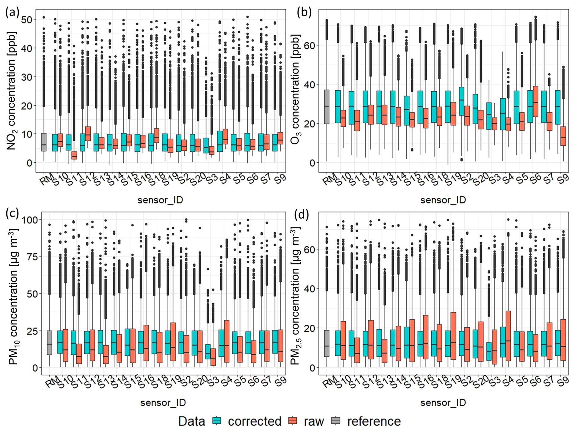
Figure 6 Box plots showing medians and ranges of (a) NO₂, (b) O₃, (c) PM₁₀ and (d) PM_2.5 hourly averaged concentrations originally measured by LCSs (raw; red colour), corrected by the MARS method (corrected; blue colour) and by the reference or equivalent method (RM; grey colour) during the initial field comparative measurement at the Prague Libuš from 16 December 2021 to 30 May 2022. Black dots show the deviated concentrations. Some weakly negative values are shown in MARS-corrected data (less than 0.3 % of the whole dataset for gases and less than 2.6 % for aerosols).

3.2 Air quality monitoring within the Legerova campaign

In the case of NO₂, which is one of the primary emission outputs from transport, the results showed a significant difference in the concentration trends measured during working days (with a high traffic intensity in the monitored streets) and during the weekends (when automotive traffic is decreased; Fig. 7). Furthermore, the effects of rush hour in the morning (from 06:00 to 09:00 UTC) and afternoon (from 15:00 to 18:00 UTC) were clearly visible during working days (Fig. 7). The highest 1 h average concentrations were measured by the most exposed LCSs during August 2022 and November 2022 (Fig. 7). Given the medians and even the averages of 1 h NO₂ concentrations, the most exposed locations were CKAIT Sokolská (at the crossroads of Sokolská and Rumunská streets), with the LCS S10 measuring a median concentration of 33.21 ppb at the higher height and the S11 measuring a median of 31.12 ppb at the lower height; Legerova (at the crossroads of Legerova and Rumunská streets), with the LCS S14 at the lower height and the S15 at the higher height, both with a median concentration of 25.13 ppb; and Rumunská, with the LCS S20 measuring a median concentration of 24.49 ppb at the lower height and S13 measuring a median of 23.34 ppb at the higher height (see Table 4, Figs. 7 and 9a). The maximum 1 h average NO₂ concentrations were 129.93 ppb measured by the LCS S12 (Sokolská school at lower height) and 92.50 ppb measured by the LCS S18 (Sokolská school at higher height; Table 4 and Fig. 9b). However, overall, according to the median and mean NO₂ concentrations, the Sokolská school site was rather moderately polluted, similar to the nearby Legerova school site (LCS S2 and S5; both sites with median concentrations ranging from 18.58 to 20.35 ppb) and the Prague Legerova RM site with the collocated LCS S4 (median concentrations of 18.82 and 20.67 ppb, respectively; Table 4, Figs. 7 and 9a). The lowest NO₂ 1 h average concentrations were measured with the background LCSs, namely the S3 placed on the roof of the Prague Karlov MS and the S16 placed on the roof of the Le Palais Art Hotel Prague (median of concentrations below 10 ppb) and further with LCSs S19 placed in the PVK garden (median concentration 11.28 ppb) and S7 placed within the closed school courtyard (median concentration 11.47 ppb; Table 4, Figs. 7 and 9a).

In the case of O₃ LCS measurement, no significant change was detected in the daily cycle of concentrations between weekdays and weekends (Fig. S40 in the Supplement). The highest O₃ concentrations were measured around midday (from 11:00 to 14:00 UTC) and, quite understandably, during the summer months (from June until August 2022; Fig. S40). The difference in the LCS-measured O₃ concentrations probably depended strongly on the individual conditions of particular locations. The highest medians of average 1 h O₃ concentrations were 13–16 ppb, measured by the LCSs S7, S18, S11 and S16 (Fig. S40), and the maximum concentrations were 103–109 ppb, measured by the LCSs S14, S20, S7 and S9 (see complete statistics in Table S20 in the Supplement). Since there is no RM for measuring O₃ available at the Prague Legerova AQM station, the data from the Prague Vysočany RM were used for indicative comparison with all LCS measurements at the Prague Legerova domain.

Measurements of aerosol particle pollution also showed a difference between weekdays and weekends. The highest 1 h average PM₁₀ and PM_2.5 concentrations were measured on Wednesdays, Thursdays and surprisingly also Sundays, while a significant drop in aerosol concentrations was detected on Saturdays (for PM₁₀, see Fig. 8, and for PM_2.5, see Fig. S41 in the Supplement). The highest concentrations were measured during the winter months (see Fig. 8). However, in general, no extremely high levels of PM₁₀ or PM_2.5 pollution were detected within the entire area of interest, despite the high traffic load in the monitored streets. LCSs S10 and S11 placed in Sokolská street (at the crossroads with Rumunská), LCSs S14 and S15 in Legerova street (at the crossroads with Rumunská), and LCSs S20 and S13 in Rumunská street were again the locations with the highest medians of 1 h average PM₁₀ and PM_2.5 concentrations ranging between 23–26 and 15–18 µg m⁻³ (respectively; see Fig. 9b, Table 5 and Fig. S41 and Table S21 in the Supplement). Conversely, the LCSs placed on the school building at the exit to the Nuselské valley and the LCSs placed in the background locations were less loaded overall (similar to the case of NO₂ pollution), with medians of measured PM₁₀ concentrations < 20 µg m⁻³ (Table 5 and Fig. 9c, Fig. S41 and Table S21). The lowest average PM₁₀ and PM_2.5 concentrations were measured by the S3 LCS placed on the roof of the Prague Karlov MS (median of PM₁₀ concentration 11.41 µg m⁻³, PM_2.5 concentration 9.14 µg m⁻³). The maximum 1 h average PM₁₀ and PM_2.5 concentrations were achieved by LCSs S5, S13, S10, RM and S2 (see Tables 5 and S21 for complete statistics) and were significantly influenced by the temporary pollution episode in July 2022 (see Sect. 3.3). The medians and maxima of NO₂ and PM₁₀ concentrations measured during the entire measurement campaign at different locations are shown in maps in Fig. 9. The difference between raw measured and MARS-corrected (COR) NO₂, O₃, PM₁₀ and PM_2.5 concentrations in all LCSs during the Legerova campaign is shown in Fig. S42 in the Supplement.

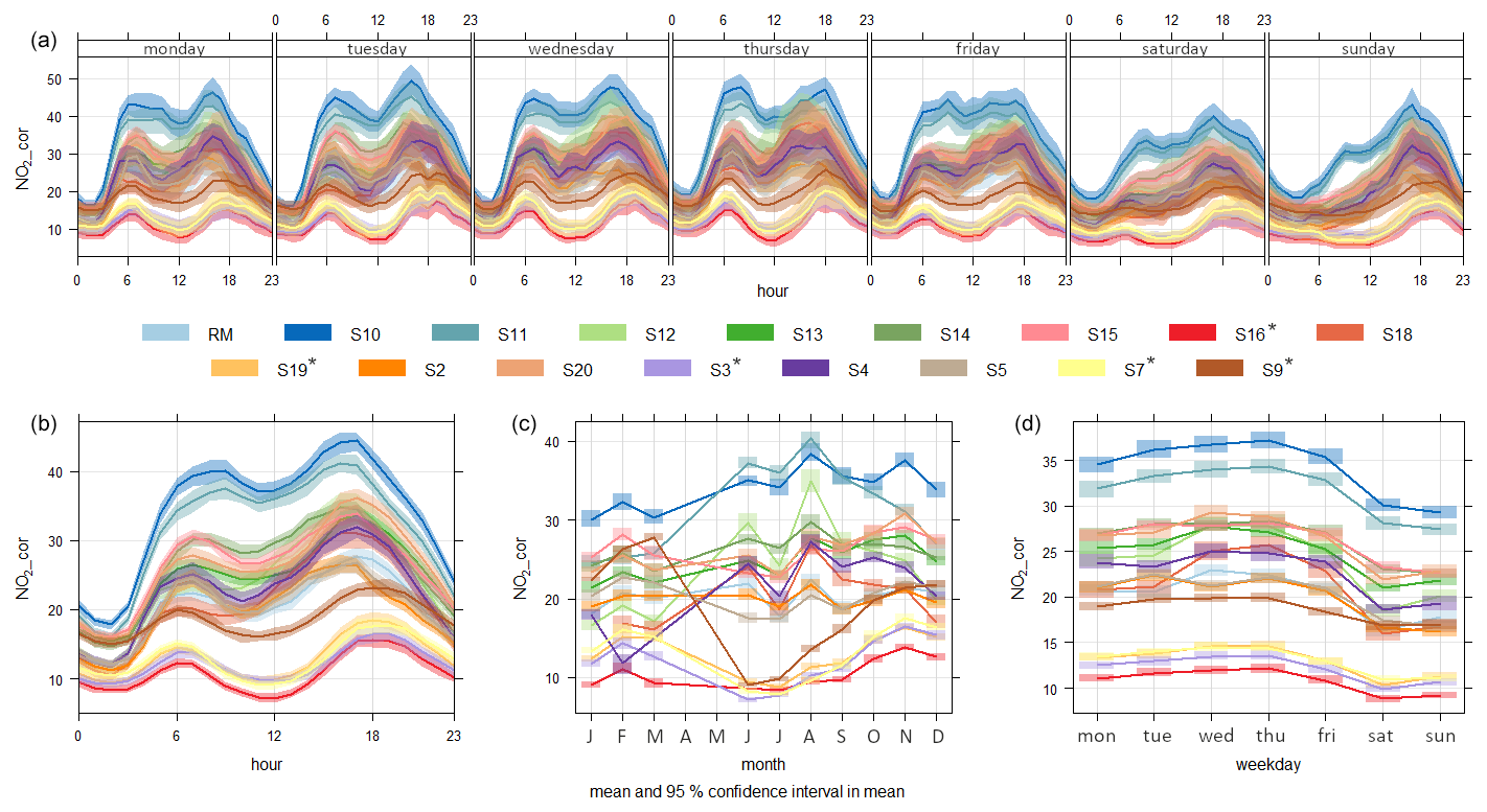
Figure 7 Daily (a), hourly (b), monthly (c) and weekly (d) corrected NO₂ concentrations (ppb) measured by all low-cost sensors (LCSs S2-S20) and by the Prague Legerova reference monitor (RM) within the Legerova campaign. Measuring period from 30 May 2022 to 28 March 2023 (in monthly graph May to December 2022, January to March 2023). LCSs located at background sites are marked with an asterisk.

Table 4 Summary statistics of 1 h average MARS-corrected NO₂ concentrations measured by all LCSs during the Legerova campaign. Valid N is the number of valid values, percentage valid is the percentage of valid values in the dataset, CI mean is the lower and upper confidence interval of the mean, Min is the minimum value, Max is the maximum value, SD is the standard deviation, CI SD is the lower and upper confidence interval of standard deviation, and SE is the standard error of the mean. The table is sorted in ascending order according to the mean concentration values. The RM and LCS S4 highlighted in bold were collocated during the campaign. LCSs located at background sites are marked with an asterisk within the ID.

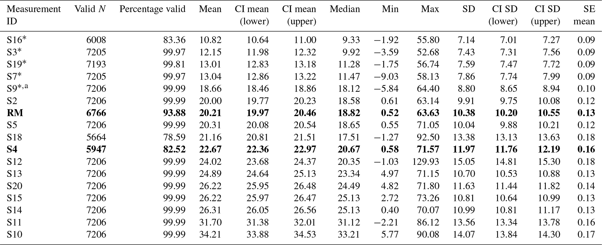
^a In the case of LCS S9, a significant data shift towards overestimation was found (flagged as a defective LCS unit that was not used for the assessment).

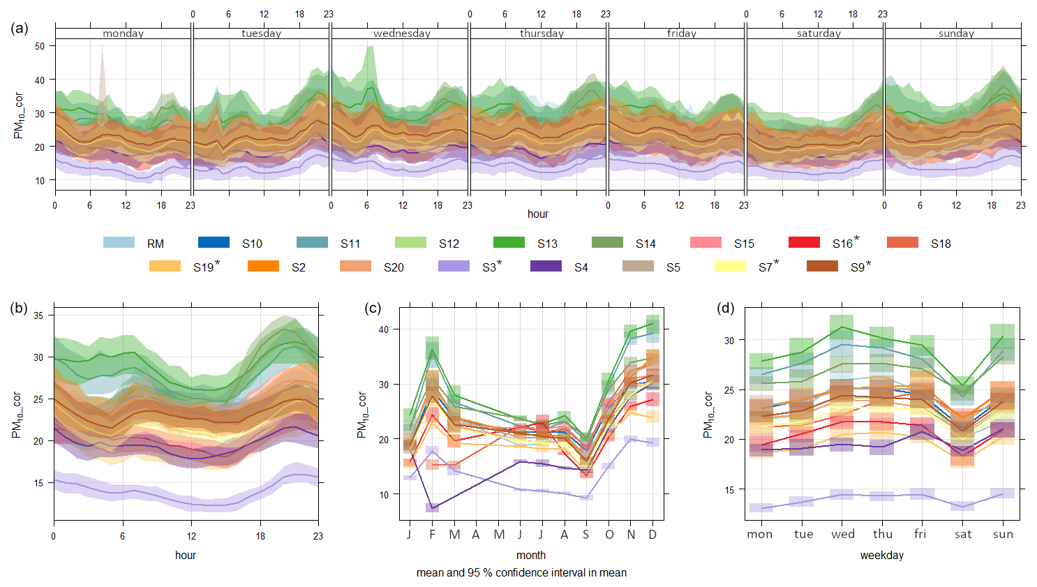
Figure 8 Daily (a), hourly (b), monthly (c) and weekly (d) variations of corrected PM₁₀ concentrations (µg m⁻³) measured by all low-cost sensors (LCSs S2–S20) and by the Prague Legerova equivalent monitor within the Legerova campaign. Measuring period from 30 May 2022 to 28 March 2023 (in monthly graph May to December 2022, January to March 2023). LCSs located at background sites are marked with an asterisk.

Table 5 Summary statistics of 1 h average MARS-corrected PM₁₀ concentrations measured by all LCSs during the Legerova measurement campaign. Valid N is the number of valid values, percentage valid is the percentage of valid values in the dataset, CI mean is the lower and upper confidence interval of mean, Min is the minimum value, Max is the maximum value, SD is the standard deviation, CI SD is the lower and upper confidence interval of standard deviation, and SE is the standard error of the mean. The table is sorted in ascending order according to the mean concentration values. The RM and LCS S4 highlighted in bold were collocated during the campaign. LCSs located at background sites are marked with an asterisk within the ID.

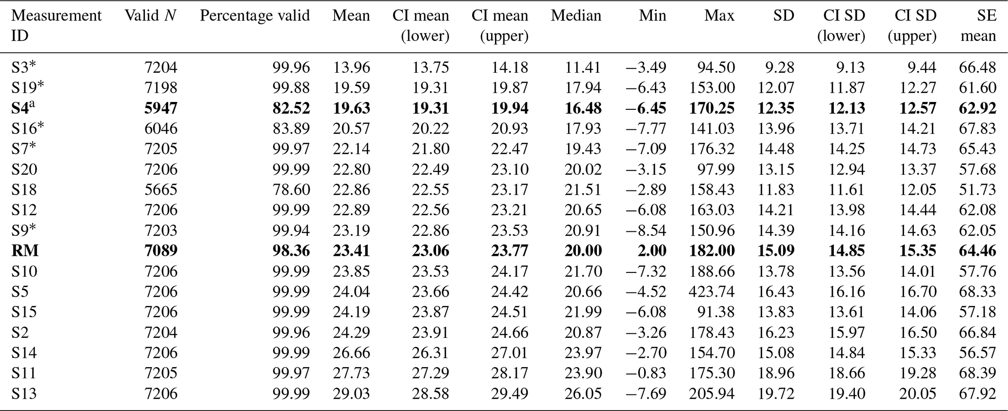
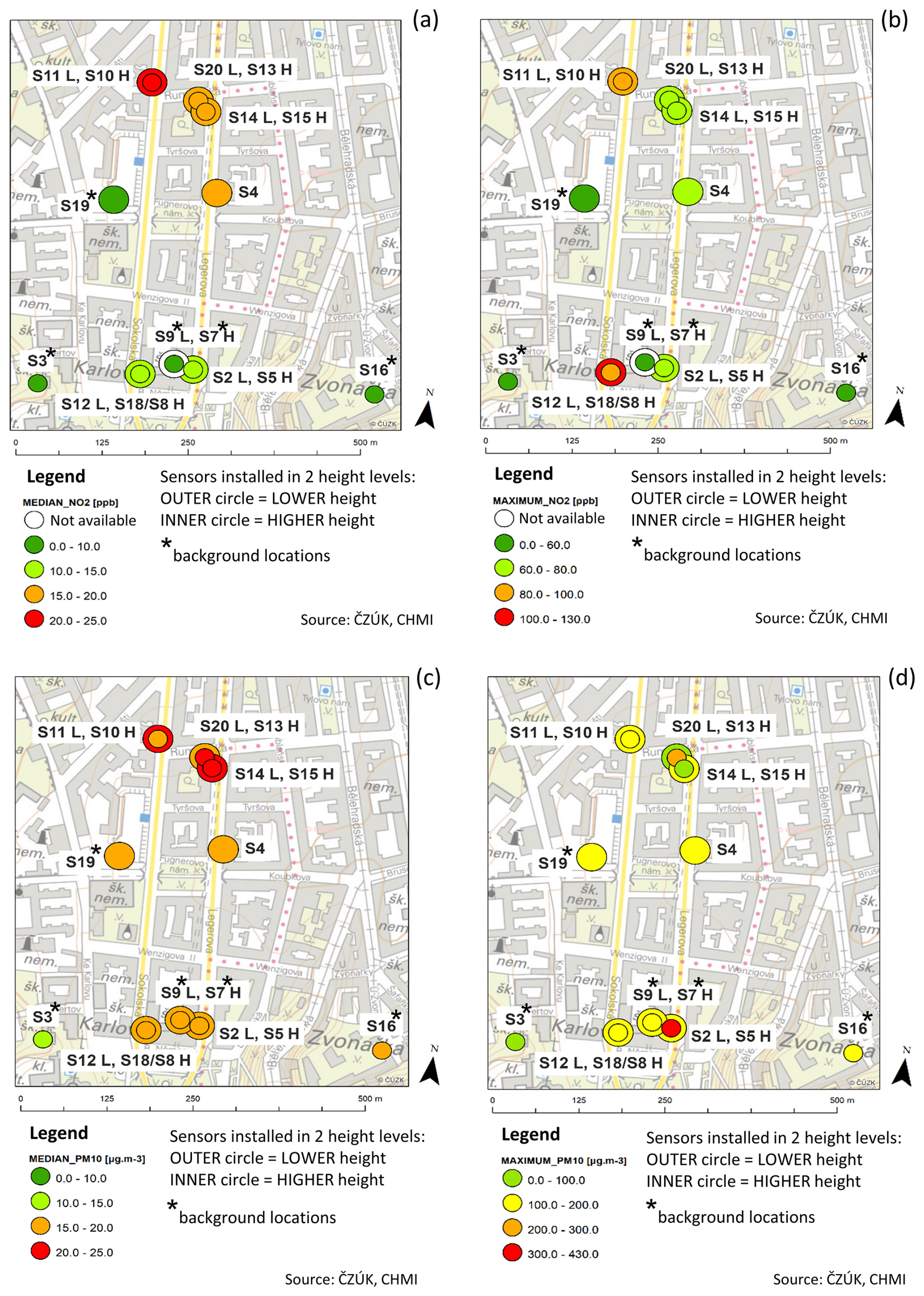
Figure 9 Map with measurement locations showing (a) median and (b) maximum NO₂ concentrations (ppb) and (c) median and (d) maximum PM₁₀ concentrations (µg m⁻³). Both were measured during the entire measurement period (from 30 May 2022 to 28 March 2023) in Legerova and its surroundings. The sensors were placed at two height levels in six locations (see legend). The colour scales differ between median and maximum concentrations and between pollutants. Background map is provided by WMS by the Czech Office for Surveying, Mapping and Cadastre – ČÚZK.

3.3 Episodes with temporarily increased air pollution concentrations

A significant pollution episode was recorded in July 2022, when a large-scale forest fire broke out in the České Švýcarsko National Park (around 90 km north of the investigated area; see map in Fig. 1a), and the aerosol pollution emitted into the air spread across the republic over long distances. On 26 July 2022, around 04:00 and 21:00 UTC, this transported aerosol pollution was also detected in Prague. Almost the entire LCS network (including background locations, with some exceptions of weaker response in LCSs S3, S15 and S20) responded accordingly, with a significant increase in PM₁₀ and PM_2.5 concentrations (see Fig. 10 and maximum concentrations in Table 5). This aerosol pollution was also detected by increased backscatter intensities from the CL51 ceilometer at Prague Karlov and from the Doppler lidar placed on the PVK roof (see Figs. S43 and S44 in the Supplement).

Otherwise, some temporary episodes with increased concentrations of PM_2.5 and PM₁₀ were measured usually during the temperature inversions, when disperse conditions had worsened, and negative values of the TMP gradient were detected from the MWR measurement (see Fig. 11 with PM_2.5 concentrations over the whole Legerova measurement campaign and Fig. 12 with examples of PM₁₀ episodes during September and December 2022 and February 2023). Similarly, short-term high concentrations of PM₁₀ and PM_2.5 occurred during New Year's Eve (see Figs. S45–S46 in the Supplement). Furthermore, in Sect. S3.2.1 of the Supplement, we present two examples of individual days with a fast and slow reconstruction of TMP stratification in the atmospheric boundary layer, corresponding well to the pollution situation, especially in the case of aerosols.

A general overview of all the meteorological measurement results is given in Sect. S3.3 in the Supplement.

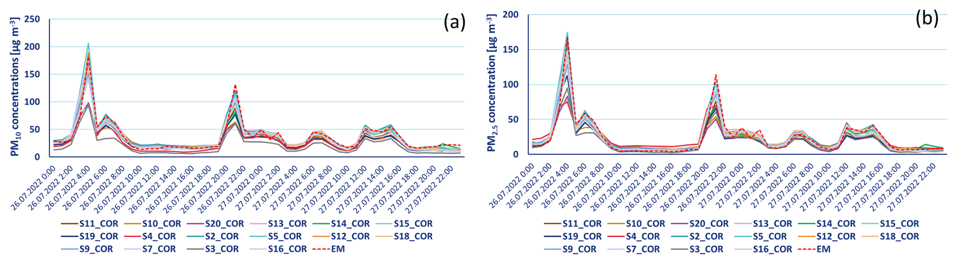
Figure 10 Concentrations of (a) PM₁₀ and (b) PM_2.5 measured by the LCS network and the Fidas equivalent monitor (EM) at the Prague Legerova AQM station during the pollution episode caused by aerosol transported from a large-scale forest fire in Hřensko (the northern part of the Czech Republic) on 26 July 2022 in the morning and evening hours.

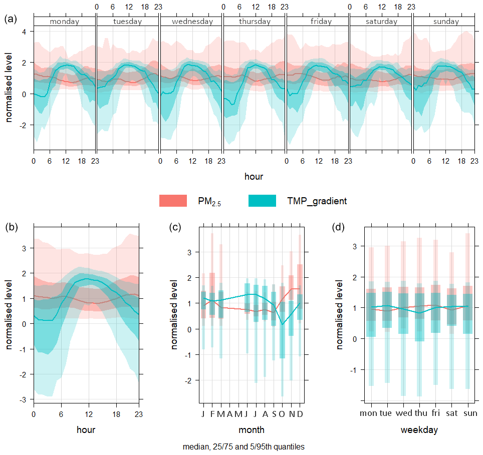
Figure 11 Daily (a), hourly (b), monthly (c) and weekly (d) variations of corrected PM_2.5 concentrations (µg m⁻³; hourly averages from all LCSs) and TMP gradient (°C per 100 m), both variables normalized for comparison. The median and quantiles are shown during the whole Legerova measurement campaign from 30 May 2022 to 28 March 2023 (in the monthly graph May to December 2022, January to March 2023).

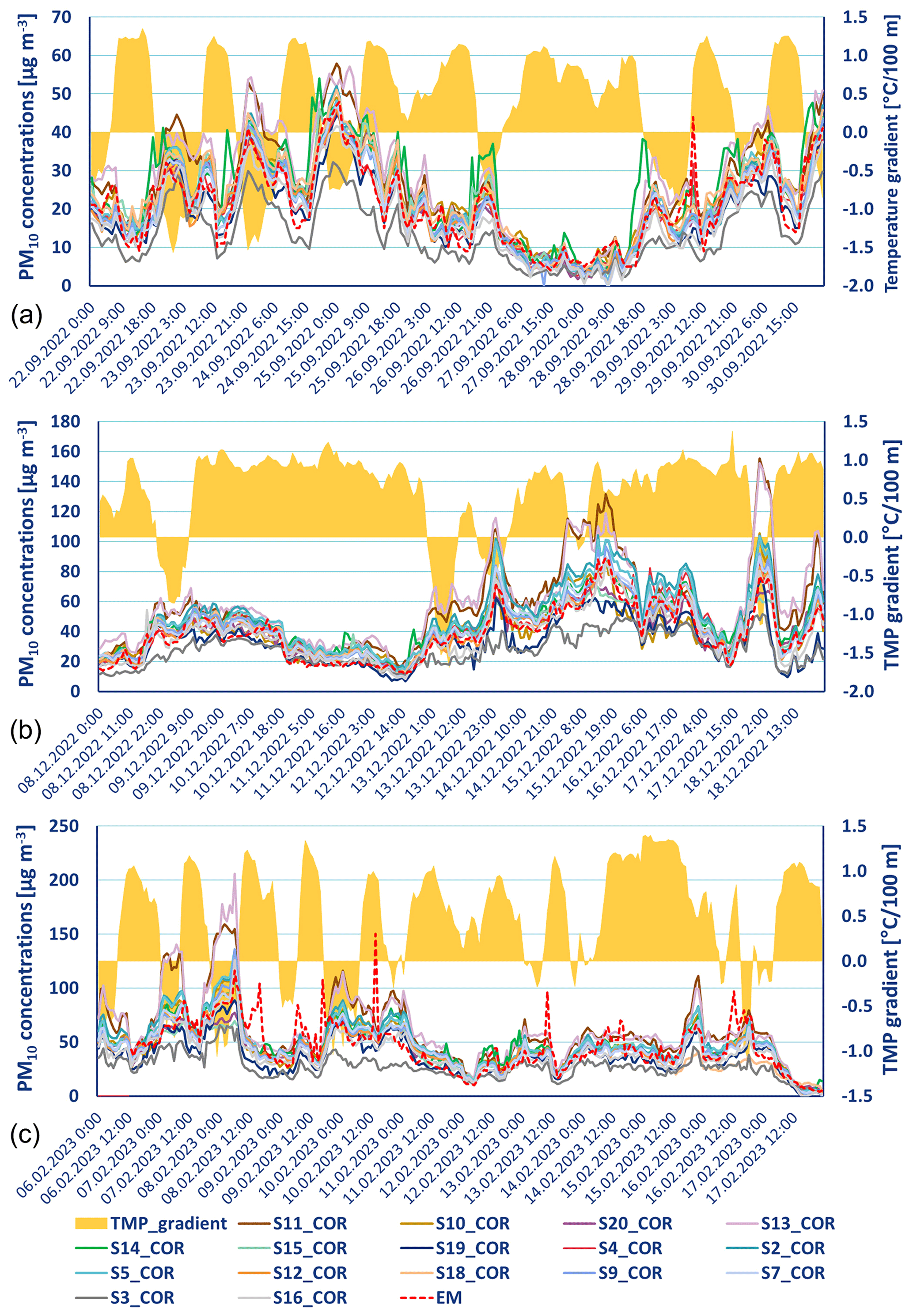
Figure 12 The course of PM₁₀ concentrations (µg m⁻³) during 22–30 September 2022 (a), 8–18 December 2022 (b) and 6–17 February 2023 (c). An increase in PM₁₀ concentrations is evident under conditions of ground temperature inversion (shown as negative temperature gradient, TMP_gradient).

4 Discussion

The discussion is structured according to the sub-topics addressed in this article.

4.1 Data quality of LCS measurement

4.1.1 Raw LCS measurement

With regard to the set study design based on the long-term initial field testing of all LCSs at the Prague Libuš AQM station (in total lasting 5.5 months), it was not sure whether all LCS units (especially the EC Cairsens NO₂ and O₃ LCSs with a stated maximum operational life of 15 months) would be able to measure data for the entire Prague Legerova campaign without failure. Finally, no major data outages or LCS malfunctions occurred with some exceptions; i.e. three EC LCSs were identified as defective at the beginning of the field test and served after repair as spare LCSs, and in the case of two LCSs, the communication unit failed during the Legerova measurement campaign (namely S18 located at Sokolská school had been broken since 13 December 2022 and was replaced by the spare S8 unit, and S4 located at the RM Legerova station had been broken since 5 February 2023; both LCSs were subsequently repaired and returned to the final field comparative measurement at the Prague Libuš station).

Evaluation of raw LCS measurement showed quite a high correlation with RM or EM for NO₂ LCSs (R² > 0.84 in all sensors) and PM₁₀ and PM_2.5 LCSs (R² > 0.72 and R² > 0.85, respectively). The weakest correlation was detected for combined ${\mathrm{O}}_{\mathrm{3}}/{\mathrm{NO}}_{\mathrm{2}}$ LCSs, with two units achieving only R²=0.52, three units R²=0.69, and the remaining units R² > 0.76 compared to the O₃ RM. However, all LCSs suffered from different zero shift (intercept shift), resulting in the following ranges of MBE: −2.98 to 4.56 ppb in NO₂, −3.41 to 14.52 ppb in O₃, −3.54 to 8.16 µg m⁻³ in PM₁₀ and −3.92 to 3.90 µg m⁻³ in PM_2.5. Especially in the case of used EC Cairsens sensors, we achieved much better results in raw measurements than in other previous studies testing these sensor types in outdoor conditions (Bauerová et al., 2020; Feinberg et al., 2018; Jiao et al., 2016; Spinelle et al., 2015). Therefore, we assume some relevant technical improvements could have been made in these sensors in recent years. Conversely, the Plantower optical particle counters used have been known for their precise lower limit of detection (range of LLOD 0.08–0.24 number of particles cm⁻³) and low susceptibility to relative humidity (Bulot et al., 2020), which results in better performance than for other types of OPCs (Bauerová et al., 2020; Bulot et al., 2020; Hong et al., 2021; Sayahi et al., 2019). Our results for PM₁₀ and PM_2.5 are consistent with those of other studies using these sensors in long-term field tests, including the slightly weaker R² for coarse PM₁₀ concentrations than for fine PM_2.5 concentrations (Bauerová et al., 2020; Hong et al., 2021; Lee et al., 2020; Sayahi et al., 2019). Overall, no significant/extreme outliers were detected in the raw gaseous or aerosol LCS measurements, either during the initial field comparative measurement, the Legerova campaign or final field comparative measurement (see maximum 1 h concentrations in Tables S12–S19 in the Supplement and Tables 4–5).

4.1.2 MARS-corrected LCS measurement

Mathematical correction using the non-parametric MARS method achieved the best results of all correction procedures tested in this study (linear regression and GAM). Pros and cons of MARS were described elsewhere (Everingham et al., 2011; Friedman 1991a, b; Hastie et al., 2009; Kuhn and Johnson, 2013; Steinberg and Colla, 1999). The superiority of the MARS methodology over other competing models has also been discussed in many publications (Leathwick et al., 2006; Lee et al., 2006; Muñoz and Felicísimo, 2004), although to our knowledge, no study has applied this method for sensor correction to date. The MARS calculation is flexible, computationally time-feasible (calculation of the model without the interactions took several seconds, with the inclusion of interactions tens of seconds) and easy to interpret and allows various explanatory variables to be taken into account, including their interactions (Friedman, 1991a; Keshtegar et al., 2018). Moreover, if the quality of the correction equations is sufficiently tested in advance (over a sufficiently wide range of meteorological conditions), no reference measurements are needed later within the sensor network to calculate the corrected concentration values. The RM is then used only for an indicative comparison of the performance of the whole sensor network over time.

To calculate the correction equations, we used the raw LCS concentrations, TMP, RH, WV, GLRD and hour of the day as the explanatory variables. Most of the previous studies used raw LCS measurement, TMP and RH (Considine et al., 2021; Cordero et al., 2018; Crilley et al., 2018; deSouza et al., 2022; Jiao et al., 2016; Malings et al., 2019; Vajs et al., 2021). Fewer studies then also included the effect of WV, air pressure or hour of the day, with mixed results (Hagler et al., 2018; Mead et al., 2013; Munir et al., 2019; Spinelle et al., 2015, 2017). In this study, the most frequently used predictors in NO₂ correction models were NO₂ raw LCS concentrations, TMP, WV and GLRD, and the least frequently used were RH and hour of the day (see Table S3 in the Supplement). In the case of O₃, the most frequently used were O₃ raw LCS concentrations, the ratio of O₃ and NO₂ LCS concentrations, TMP, RH and WV; on the other hand, GLRD and hour of the day were, quite surprisingly, the least used predictors (Table S5). In the PM measurement (both PM₁₀ and PM_2.5), the most frequently used were raw LCS concentrations and then all other predictors with a similar weight. Here again, quite surprisingly, the RH was not a dominant predictor in PM correction equations (see Tables S7 and S9 in the Supplement). Double interactions between variables were ultimately not included in the corrections, as they led to significant outliers in both gaseous and aerosol measurements (especially at high peak concentrations). Nevertheless, MARS corrections decreased MBE to nearly zero for all measured pollutants in all cases. The MARS corrections improved the relationships with RMs or EMs with an average R²=0.97 in NO₂, 0.94 in O₃, 0.87 in PM₁₀ and 0.94 in PM_2.5. The average of generalized cross-validation (GCV) error of the MARS correction models was the lowest (1.14) in NO₂ LCS corrections and the highest (27.54) in PM₁₀ LCS corrections. Comparing the results of NO₂ and O₃ MARS corrections with the performance of other statistical correction models (MLR, RF or ANN) in previous studies, we achieved better or similar results (according to R² resulting from linear regression between reference data and corrected LCS data; e.g. maximum R²=0.75 with the MLR model in Spinelle et al., 2015, R²=0.97 with the RF model in Cordero et al., 2018). In the case of aerosol particles, Vajs et al. (2021) achieved better results (R² > 0.90) in the correction of PM₁₀ LCS measurement with different ANN or RF models, and Kumar and Sahu (2021) achieved slightly better results (R²≥0.98) in PM_2.5 LCS measurement with KNN, RF, regression tree (RT) or GB methods. Conversely, Vogt et al. (2021) achieved worse results for both PM₁₀ and PM_2.5 in the case of correction with sensor-specific linear models (highest R² values 0.64 for PM₁₀ and 0.73 for PM_2.5), similar to Kumar and Sahu (2021) with MLR correction (R²=0.77) and Hong et al. (2021) with non-linear regression (R² > 0.88), both in PM_2.5 measurement.

Very similar results were achieved when comparing the two correction procedures COR (based on initial comparison) and COR2 (based on initial and final comparison, including sensor ageing). However, the diversity of applications must be taken into account. While the COR method can be used to correct operationally measured LCS data, COR2 can be applied only retroactively after the end of the entire measurement campaign.

4.1.3 LCS data drift evaluation

The issue of data drift detection has been addressed in various studies. Malings et al. (2019) describe the drift adjustment based on the method of “deployment records”, using the biases between LCS and RM measurements during collocation (before deployment). The LCS with the lowest bias is identified as a “benchmark” sensor, which is collocated for the entire measurement period. Any subsequent possible non-standard deviations in the LCS measurement network were then assessed against the bias of this benchmark sensor. This method is useful; however, it assumes that the bias is generalizable/transferable across all LCS units, which is not always the truth due to the high differences in LCS measurement precision (De Vito et al., 2020; van Zoest et al., 2019). Harkat et al. (2018) described a much more challenging and complex framework consisting of air quality modelling, fault detection, fault isolation and reconstruction to set the boundaries for probable and improbable LCS measurements (using a combination of midpoint-radii principal component analysis (PCA), generalized likelihood ratio test and exponentially weighted moving average for detecting changes in the LCS model residuals). A simpler technique was described by van Zoest et al. (2019) where the control of LCS drifts was based on the time series of the difference/bias between the mean NO₂ concentrations measured by RMs placed within the area of interest and mean NO₂ concentrations measured by all LCSs in the network. A zero difference was not expected here because the LCSs were differently spaced, and the difference may be subject to NO₂ seasonality and meteorological conditions. However, when the difference/bias began to systematically decrease or increase regardless of changes in conditions, the data drift could be indicated.

As part of this study, we tried to apply similarly simple and effective data control methods, targeting the possible data drifts caused either by relocation of the LCS stations to target deployment sites, by technical failures of the LCSs (e.g. ageing) or by loss of the MARS correction performance (the concept drift). Firstly, all measurements were checked by the mutual comparison of the concentration courses of LCSs located in pairs (also including the two collocated LCSs with RMs); secondly, by the DMC method to check the data continuity; and thirdly, by the final field comparative measurement carried out at the Prague Libuš AQM station. The control within pairs of LCSs or in between collocated LCS S4 and RM did not show any deviations after the relocation of the LCSs to the final deployment sites. The change in measurement performance was visually detected a few months later in the case of the NO₂ S9 LCS, which drifted to gradual overestimation from September 2022 (similar to that detected in the PM sensor in Sayahi et al., 2019). This was probably caused by a technical issue (different aspects discussed in Weissert et al., 2019) because the data drift was detected in both raw and corrected concentrations. This data drift was later confirmed by the DMC analysis and by final comparative field measurement (final intercept 16.43, slope 0.61, R²=0.17, MBE = −14.39). The NO₂ S9 LCS measurement was therefore marked as invalid and was not further used for the Legerova campaign evaluation. Another two NO₂ LCSs had weaker performance during the final comparative measurement, namely S4 and S3 (with values of R² 0.58 and 0.76, intercept 5.67 and 4.60, slope 0.97 and 0.84, and MBE −5.48 and −3.77, respectively). Two LCSs were further identified based on DMC as cases of possible drift to gradual underestimation, the S11 and S12. In these cases, the data drifts were not as significant as in the S9, and during the final comparative measurement, these LCSs still performed well (R² > 0.81, intercept ∼ 2.82, slope 0.79 and 0.94, MBE −1.70 and −2.54, respectively; see Table S16 and Fig. S29 in the Supplement). A possible reason for the drop in LCSs' performance could be the loss of sensitivity of the electrochemical cell (see van Zoest et al., 2019).

In O₃ LCS measurement, a technical problem was most likely detected, as a sudden data drift (in the sense of jump to overestimation) was recorded for all LCSs from October to November 2022 (Fig. S26 in the Supplement). Since this phenomenon also appeared in the raw measurement, the drift of the correction concept can be ruled out (De Vito et al., 2020; Spinelle et al., 2015). During October 2022 a rapid change in air temperature (with a drop below 4 °C) occurred, which may have triggered this change in LCS measurement performance (although the correction model was trained for winter conditions; Weissert et al., 2019). In the case of aerosol measurement, no gradual or sudden data drifts were detected during the Legerova campaign, not even during the final comparative measurement. One exception was the PM LCS S3, which was already partly underestimating data from the start of measurement (see corrected PM₁₀ and PM_2.5 concentrations in Fig. 6). Since this LCS had a shortened initial comparison measurement time compared to the other LCSs (installed on the roof of the Karlov MS since 23 February 2022), it could be the result of an under-trained MARS correction model. However, the PM data from the S3 LCS were not marked as invalid, only as permanently underestimated (see Fig. 8), because it was not typical data drift as described above (no change of measurement performance detected during the campaign). Although no major data drifts were observed in the case of PM₁₀ and PM_2.5 measurements, it should be noted that all sensors had weaker performance during the final comparative measurement. In the case of PM₁₀ the resulting range of R² was 0.47–0.63 and of MBE was −4.40 to 4.80; in the case of PM_2.5 measurements, R² was 0.77–0.89 and MBE was −4.44 to 1.20 (see Tables S18–S19 in the Supplement).

4.2 Air quality and meteorological measurement within the Legerova campaign

The results of the almost year-long observation campaign in Legerova, Sokolská and Rumunská streets and their surroundings showed that the largest load in this area is NO₂ pollution, due to the high daily traffic within this selected area of the city centre of Prague (with the following intensity of cars per day: 37 336 in Sokolská, 35 736 in Legerova and 9608 in Rumunská; TSK, 2023). Therefore, the daily and weekly courses of NO₂ concentrations corresponded well to the traffic regime in the given localities (with typical morning and late-afternoon rush hour peaks of concentrations), including the lower concentrations in background locations more distant from the emission sources (Fig. 9). The highest NO₂ concentrations in medians and averages behaved according to the expectations in street canyons with continuous building blocks and several traffic lights (LCSs S10 and S11 in Sokolská, S14 and S15 in Legerova, and S20 and S13 in Rumunská). Locations with more open space nearby, i.e. with a higher probability of ventilation effect, came out as moderately loaded (LCSs S12 and S18 in Sokolská school, S2 and S5 in Legerova school, and S4 collocated with the Prague Legerova RM). Nevertheless, the maximum 1 h average NO₂ concentrations were measured by LCSs S12 and S18 placed in the Sokolská school location (Fig. 9b). Since the maximum concentration peaks were measured by both LCSs installed at different height levels, we assume that this was a reflection of some real local emission effect (e.g. a started supply car standing near the LCSs) and the random LCS error can be ruled out. The mean and maximum NO₂ concentrations measured within the most loaded locations during the Legerova campaign in Prague were comparable to the study of Schneider et al. (2017) focused on monitoring traffic-polluted urban sites in Oslo (FI), where the measured concentrations ranged between 42 and 63 ppb, or Moltchanov et al. (2015) in the city of Haifa (IL), with concentration peaks ranging between 50–95 ppb. On the other hand, our measurements were higher than those of Graça et al. (2023) in the city of Aveiro (PT), with NO₂ concentrations between 15 and 32 ppb, or those of Wesseling et al. (2019), measuring around 15 ppb in Amsterdam or Utrecht (NL). However, these comparisons are only indicative due to different conditions in cities.

Other interesting results within the Legerova observation campaign were reached in the case of aerosol pollution measurement. Although some daily patterns were recognizable in PM₁₀ and even in PM_2.5 concentrations, the concentration peaks, especially during the late afternoon, were shifted to later than the usual rush hours. The concentration peaks of NO₂ were observed between 15:00 and 18:00 UTC, while the PM₁₀ and PM_2.5 concentration peaks usually occurred between 17:00 and 21:00 UTC (see Fig. S56 in the Supplement for details). Overall there were quite low levels of PM pollution and smaller differences between different sites within the whole area of interest (medians of PM₁₀ ranging between 11 and 26 µg m⁻³ and PM_2.5 between 9 and 18 µg m⁻³). According to the measured aerosol concentrations, the most burdened locations (with medians of PM₁₀>23 µg m⁻³) were LCSs S13 (in Rumunská), S11 (in Sokolská) and S14 (in Legerova; similar to NO₂ pollution) and the least burdened were the background LCSs S3, S16, S19 and surprisingly even the S4 collocated with the Prague Legerova RM (with medians < 18 µg m⁻³; see Fig. 9c and d). Similarly low levels of PM₁₀ and PM_2.5 concentrations were measured in the city of Aveiro by Graça et al. (2023) and in Nantes (FR) by Gressent et al. (2020). These results may suggest that with the current development of cars in recent years, transport might not be the main source of aerosol pollution in European cities, unlike nitrogen oxides (see for example Scerri et al., 2023). Transport can produce particles of a smaller size fraction (PM_2.5, PM₁ and smaller), which can be emitted from the incomplete combustion of engines and emissions from brake and tire abrasion, which are part of PM_2.5 and larger size fractions. However, in both cases, the contribution of these sources forms a very small part of the total PM pollution from transport. A significant part of the pollution here is made up of coarse particles (PM₁₀ and larger), which settle on the road surface for a long time and are subject to resuspension (secondary dust from traffic; the amount of specific types of emissions from transport in the Sokolská and Legerova streets is shown in Fig. S57 in the Supplement). This also explains the similarity of PM₁₀ concentration trends and only slightly higher values of concentrations measured at the Prague Legerova RM and other rather background AQM stations in Prague that are less loaded with traffic (see Fig. S58 in the Supplement). The highest aerosol pollution (PM₁₀>130 µg m⁻³ and PM_2.5>110 µg m⁻³) was measured temporarily in all LCS stations during the early-morning and late-evening hours on 26 July 2022 according to the transported pollution from the Hřensko forest fire (a similar situation was detected even in other parts of the Czech Republic).

Similarly, as in Frederickson et al. (2024), we had some difficulty in demonstrating the vertical gradient pollution effect from the LCS measurement installed at two height levels. Therefore, higher concentrations were not always measured at low heights closer to the emission sources but sometimes even at a higher height above the ground. The vertical concentration profiles depend mainly on atmospheric stratification, street architecture, air flow and surface properties (Frederickson et al., 2024). In connection with the atmospheric stratification, we observed high PM₁₀ and PM_2.5 concentrations (i.e. > 40 µg m⁻³) especially under temperature inversion conditions, even at night. From this point of view, the level of aerosol pollution was more influenced by atmospheric stratification than NO₂ pollution, which was more subject to the traffic regime in the streets. Therefore, we also showed a few examples of vertical stratification reconstructions and low-level jets monitored above the area of interest under temperature inversion conditions (using the Doppler lidar and MWR measurement). Similar continuous TMP and wind vertical profile data above the urban surface are not as common (Allwine et al., 2002; Kallistratova and Kouznetsov, 2012; Sánchez et al., 2022) and are very useful in supporting advanced modelling and assessment of the impacts of air pollution and climate change in the urban environment.

5 Conclusions

This study evaluated the performance of low-cost sensors (LCSs) in monitoring air quality, with a specific focus on the application of MARS correction, the overall performance of the LCS network and methods of data quality control.

The application of the MARS correction method proved to be highly effective, offering significant improvements in measurement accuracy for all observed pollutants. Compared to alternative correction models such as linear regression and GAM analyses, MARS demonstrated superior performance due to its flexibility, computational efficiency, and ability to incorporate multiple explanatory variables and non-linear relationships in the data. Notably, the method reduced biases and brought measurement accuracy to levels comparable to, or better than, other state-of-the-art correction models (like artificial neural networks or random forests) in previous studies. However, its dependence on high-quality initial field-calibration data and the potential challenges in addressing concept drifts over time remain key limitations.

The LCS network demonstrated robust performance throughout the measurement campaign, with minimal data outages and consistent results across most sensors. Nevertheless, several LCS units exhibited gradual or sudden data drifts, primarily due to sensor ageing or technical issues. These were effectively identified and addressed using a combination of methods, including within-pair comparisons, data continuity monitoring (double mass curve (DMC) method) and final comparative measurements. While these methods proved practical and efficient, their accuracy still depends on indicative validation against reference monitors (placed at different distances from the sensors).

The Legerova campaign revealed that nitrogen dioxide (NO₂) pollution posed the most significant burden in the monitored area due to intense traffic, with peak concentrations corresponding to morning and evening rush hours. Median NO₂ levels were highest in street canyon locations with limited ventilation and near traffic lights, such as Sokolská and Legerova streets. Particulate matter concentrations (PM₁₀ and PM_2.5) showed less spatial and temporal variability, with peaks often occurring later in the day and at night, particularly under the influence of temperature inversions and poor dispersion conditions. Supplementary meteorological measurements, such as those capturing vertical stratification and airflow, were crucial for interpreting pollution dispersion patterns and understanding the impact of atmospheric dynamics on local air quality.

Overall, the findings affirm the potential of MARS-corrected LCS networks as a cost-effective solution for air quality monitoring, especially in urban areas. However, addressing challenges such as sensor ageing, concept drift and the robustness of correction models under varying environmental conditions is essential for their broader application. The data obtained in this study were used to evaluate and test the sensitivity of various urban modelling tools (Resler et al., 2024; Patiño et al., 2024) and can be further used to validate microscale urban models.