Critical load exceedances for North America and Europe using an ensemble of models and an investigation of causes of environmental impact estimate variability: an AQMEII4 study

Exceedances of critical loads for deposition of sulfur (S) and nitrogen (N) in different ecosystems were estimated using European and North American ensembles of air quality models, under the Air Quality Model Evaluation International Initiative Phase 4 (AQMEII4), to identify where the risk of ecosystem harm is expected to occur based on model deposition estimates. The ensembles were driven by common emissions and lateral boundary condition inputs. Model output was regridded to common North American and European 0.125° resolution domains, which were then used to calculate critical load exceedances. Targeted deposition diagnostics implemented in AQMEII4 allowed for an unprecedented level of post-simulation analysis to be carried out and facilitated the identification of specific causes of model-to-model variability in critical load exceedance estimates.

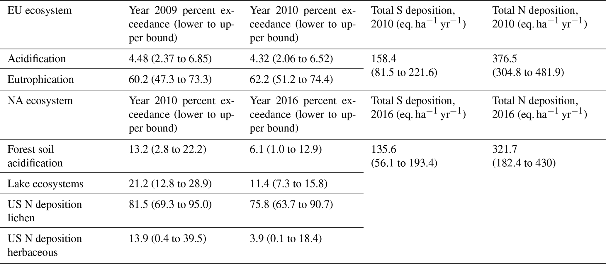
Datasets for North American critical loads for acidity for forest soil water and aquatic ecosystems were created for this analysis. These were combined with the ensemble deposition predictions to show a substantial decrease in the area and number of locations in exceedance between 2010 and 2016 (forest soils: 13.2 % to 6.1 %; aquatic ecosystems: 21.2 % to 11.4 %). All models agreed regarding the direction of the ensemble exceedance change between 2010 and 2016. The North American ensemble also predicted a decrease in both the severity and total area in exceedance between the years 2010 and 2016 for eutrophication-impacted ecosystems in the USA (sensitive epiphytic lichen: 81.5 % to 75.8 %). The exceedances for herbaceous-community richness also decreased between 2010 and 2016, from 13.9 % to 3.9 %. The uncertainty associated with the North American eutrophication results is high; there were sharp differences between the models in predictions of both total N deposition and the change in N deposition and hence in the predicted eutrophication exceedances between the 2 years. The European ensemble was used to predict relatively static exceedances of critical loads with respect to acidification (4.48 % to 4.32 % from 2009 to 2010), while eutrophication exceedance increased slightly (60.2 % to 62.2 %).

While most models showed the same changes in critical load exceedances as the ensemble between the 2 years, the spatial extent and magnitude of exceedances varied significantly between the models. The reasons for this variation were examined in detail by first ranking the relative contribution of different sources of sulfur and nitrogen deposition in terms of deposited mass and model-to-model variability in that deposited mass, followed by their analysis using AQMEII4 diagnostics, along with evaluation of the most recent literature.

All models in both the North American and European ensembles had net annual negative biases with respect to the observed wet deposition of sulfate, nitrate, and ammonium. Diagnostics and recent literature suggest that this bias may stem from insufficient cloud scavenging of aerosols and gases and may be improved through the incorporation of multiphase hydrometeor scavenging within the modelling frameworks. The inability of North American models to predict the timing of the seasonal peak in wet ammonium ion deposition (observed maximum was in April, while all models predicted a June maximum) may also relate to the need for multiphase hydrometeor scavenging (absence of snow scavenging in all models employed here). High variability in the relative importance of particulate sulfate, nitrate, and ammonium deposition fluxes between models was linked to the use of updated particle dry-deposition parameterizations in some models. However, recent literature and the further development of some of the models within the ensemble suggest these particulate biases may also be ameliorated via the incorporation of multiphase hydrometeor scavenging. Annual sulfur and nitrogen deposition prediction variability was linked to SO₂ and HNO₃ dry-deposition parameterizations, and diagnostic analysis showed that the cuticle and soil deposition pathways dominate the deposition mass flux of these species. Further work improving parameterizations for these deposition pathways should reduce variability in model acidifying-gas deposition estimates. The absence of base cation chemistry in some models was shown to be a major factor in positive biases in fine-mode particulate ammonium and particle nitrate concentrations. Models employing ammonia bidirectional fluxes had both the largest- and the smallest-magnitude biases, depending on the model and bidirectional flux algorithm employed. A careful analysis of bidirectional flux models suggests that those with poor NH₃ performance may underestimate the extent of NH₃ emission fluxes from forested areas.

Model–measurement fusion in the form of a simple bias correction was applied to the 2016 critical loads. This generally reduced variability between models. However, the bias correction exercise illustrated the need for observations which close the sulfur and nitrogen budgets in carrying out model–measurement fusion. Chemical transformations between different forms of sulfur and nitrogen in the atmosphere sometimes result in compensating biases in the resulting total sulfur and nitrogen deposition flux fields. If model–measurement fusion is only applied to some but not all of the fields contributing to the total deposition of sulfur or nitrogen, the corrections may result in greater variability between models or less accurate results for an ensemble of models, for those cases where an unobserved or unused observed component contributes significantly to predicted total deposition.

Based on these results, an increased process-research focus is therefore recommended for the following model processes and for observations which may assist in model evaluation and improvement: multiphase hydrometeor scavenging combined with updated particle dry-deposition, cuticle, and soil deposition pathway algorithms for acidifying gases, base cation chemistry and emissions, and NH₃ bidirectional fluxes. Comparisons with satellite observations suggest that oceanic NH₃ emission sources should be included in regional chemical transport models. The choice of a land use database employed within any given model was shown to significantly influence deposition totals in several instances, and employing a common land use database across chemical transport models and critical load calculations is recommended for future work.

1 Introduction

The concept of a critical load (CL) was first proposed as a means for evaluating the ecosystem impacts of the deposition of sulfur and nitrogen in response to the Convention on Long-Range Transboundary Air Pollution (CLRTAP), an international agreement on the mitigation and control of acidifying pollution, which entered into force in 1983 (CLRTAP, 2023). The convention provided some of the initial impetus for the development of comprehensive air quality models. The models provide a means of estimating the deposition fluxes of sulfur- and nitrogen-containing chemicals of anthropogenic origin, which may then be used to estimate the corresponding ecosystem impacts. Critical load exceedance estimates are the broadly accepted methodology for estimating the potential for ecosystem harm related to acidification and eutrophication. A critical load in this context was defined (Nilsson and Grennfelt, 1988) as “A quantitative estimate of an exposure to one or more pollutants below which significant harmful effects on specified sensitive elements of the environment do not occur, according to present knowledge”. This definition is parsed in detail for readers unfamiliar with the critical load concept, in the Supplement.

The creation of critical loads for acidification and the calculation of their exceedances are based on the concept of the chemical charge balance steady state within soil water or aquatic ecosystems. The fluxes of anions and cations entering or leaving an ecosystem are used to determine whether an excess cation flux is available to the ecosystem, which could balance anion fluxes associated with acidifying deposition. Anion fluxes added to the system from anthropogenic sources include forms of deposited sulfur and nitrogen noted above. The S-containing forms of deposition (S_dep) are assumed to rapidly oxidize and are treated within critical load calculations as the sulfate ion. Every mole of deposited sulfur is assumed to be associated with two negative charges as the sulfate ion, SO${}_{\mathrm{4}}^{\mathrm{2}-}$(aq) (aqueous); hence the deposition flux is tracked as charge equivalents per hectare per year, eq. ha⁻¹ yr⁻¹. N-containing forms of deposition (N_dep) are assumed to rapidly oxidize and are treated as the nitrate ion – every mole of deposited nitrogen (including those of ammonia and ammonium) is assumed to be associated with one negative charge of nitrate ion deposition, NO${}_{\mathrm{3}}^{-}$(aq). Base cations and their deposition (Ca²⁺, Mg²⁺, K⁺, and Na⁺) are included in critical load calculations (collectively, BC_dep) and may incorporate anthropogenic base cation fluxes. The anthropogenic deposition fluxes in the ecosystem from the atmosphere are used in calculations of critical load exceedances. The critical loads themselves include estimates of natural atmospheric fluxes as well as other terms for fluxes of anions and cations. For example, in the steady-state or simple mass balance (SMB) model often used to define surface water critical loads for terrestrial ecosystems (Sverdrup and de Vries, 1994), BC_dep includes the release of soil base cations due to weathering, non-marine chloride deposition, the harvesting of base cations and/or nitrogen-containing biomass, denitrification, nitrogen immobilization in the rooting zone, the runoff volume, and a critical value of the non-sodium base cation to the aluminum ion ratio. Aquatic-ecosystem critical loads with respect to acidity are usually calculated using the steady-state water chemistry (SSWC) or the first-order acidity balance (FAB) methodologies (Henriksen and Posch, 2001; CLRTAP, 2023; de Vries et al., 2015) or other similar approaches (McDonnell et al., 2014). The SSWC model makes use of the difference between an estimate of the sea-salt-corrected pre-acidification concentration of base cations in the surface water and a specified biological indicator species' acid-neutralizing capacity limit above which no significant damage is expected to occur. The FAB methodology assumes the runoff fluxes at a lake outlet are charge-balanced and relates these runoff terms to fluxes of ions entering the lake and dimensionless retention factors and to terms for nitrogen immobilization, nitrogen growth uptake into vegetation, denitrification, atmospheric deposition, and weathering. An overview of the above methods for critical load (CL) estimation and how they are used in estimating exceedances may be found in CLRTAP (2023), Makar et al. (2018), and the references therein.

Critical loads of nutrient nitrogen and their exceedances are used to address the issue of the influx of airborne nitrogen resulting in changes in soil-based processes, plant growth, and inter-species relationships. Nitrogen-containing gases and aerosol components may be directly toxic to sensitive individual plant and animal species, while the accumulation of nitrogen (increased nitrogen availability) may also change species composition or relative abundance. Soil-mediated effects of acidification may include eutrophication, and species may have increased susceptibility to secondary stressors such as drought, frost, pathogens, or herbivores (CLRTAP, 2023). Critical loads of the eutrophication processes associated with nutrient nitrogen in terrestrial ecosystems may also make use of a version of the SMB model. This critical load model balances the input fluxes of all forms of nitrogen deposition plus biological fixation and soil nitrogen adsorption against ecosystem nitrogen losses (immobilization in soil organic matter, removal via harvesting of vegetation and animals, fluxes to the atmosphere (denitrification), erosion, combustion, ammonia volatilization, and leaching below the root zone). Biological fixation, soil adsorption, combustion, erosion, and ammonium leaching are usually considered negligible, and denitrification is assumed to be linearly dependent on the net input of nitrogen, leading to critical loads of nutrient nitrogen dependent only on immobilization, harvesting removal, the acceptable limit for nitrogen leaching of sensitive plant or animal species (nitrogen in soil water), and an ecosystem-dependent denitrification fraction (CLRTAP, 2023). The acceptable limits for nitrogen concentrations in soil can range from 6.5 down to 0.2 mg N L⁻¹, depending on the vegetation type (CLRTAP, 2023). A further means of estimating eutrophication is via comparison of measured nitrogen deposition with observed ecosystem damage over a large number of sites (Geiser et al., 2019; Simkin et al., 2016). Exceedances for eutrophication in this case may be estimated as the differences between the estimated nitrogen deposition and the observation-based critical load.

As noted in the Supplement, critical load exceedance calculations are carried out on an ongoing basis due to the ongoing cycle of chemical transport model (CTM) process improvement. The results of our analyses should thus be considered a “snapshot” of the state of both CTM science and critical load (CL) knowledge at the time the simulations and critical load data collection took place (2021). CTMs numerically integrate the system of time-dependent differential equations describing the rates of change in chemical species in the atmosphere in order to predict the changes in chemical concentrations and deposition over time. This is usually done by breaking the net differential equation for the rates of change into component processes (e.g. advection, diffusion, gas-phase chemistry, inorganic particle chemistry, dry deposition, particle microphysics treating the nucleation, condensation of gases, coagulation of particles, cloud processing of gases and aerosols including wet deposition), with the processes being solved in sequence to determine the future state of the atmosphere (Marchuk, 1990). However, there is usually not a complete scientific consensus on the best numerical methods to carry out the time stepping for each of these processes, and the level of detail in process representation in the models may also vary considerably, depending at times on external constraints such as the processing time available for CTM simulations. The individual processes are usually evaluated based on laboratory or other process-specific data wherever possible, but the selection of a specific process representation within a CTM is often based on comparisons of the output of an entire CTM relative to surface or satellite monitoring data. This latter approach may allow for the compensation errors in the process representation to take place (cf. Makar et al., 2014; Hyder et al., 2018; Huang et al., 2021; Vizuete et al., 2022). These considerations may contribute to the resulting variability in deposition estimates from the different modelling frameworks. The work conducted here uses analysis of new model diagnostic outputs added for AQMEII4 to attempt to determine the key causes of these model deposition estimate differences.

The ongoing reevaluation and improvement of CTMs is aided by ensemble model comparisons, where models driven by the same lateral boundary and emission inputs are cross-compared and evaluated against observations. The Air Quality Model Evaluation International Initiative (AQMEII) has comprised model CTM ensemble evaluation studies, to date in four phases. The initial phase of AQMEII utilized largely offline regional models used for research and public policy support to simulate a common year, 2006, with common emission inputs, in both North America (NA) and Europe (EU), with 22 modelling groups participating (Galmarini et al., 2012). Subsequent phases of AQMEII examined specific issues within the CTM community: AQMEII2 had as its focus the evaluation of both weather and air quality predictions for fully coupled, online air quality models, where the particulate matter generated by the models on any given time step feeds back into the coupled models' weather forecast radiative transfer and cloud formation processes (Galmarini et al., 2015). AQMEII3 addressed questions of hemispheric transport of air pollutants – the relative contributions of local versus long-range transport to predicted pollutant concentrations, and their impacts on ecosystem and human health (Galmarini et al., 2017).

The variety in underlying scientific theory encapsulated within CTMs and their process representation implies the need for cross-comparison of critical load exceedance predictions from a variety of models. As part of AQMEII3, 14 air quality models were used to calculate oxidized sulfur and oxidized and reduced nitrogen deposition, and hence critical load exceedances in Europe (Vivanco et al., 2018). This comparison revealed a high degree of variability in simulated wet- and dry-deposition fluxes. The models with the best performance relative to observations were used to provide ensemble critical loads – a “reduced ensemble” in that not all models submitting output for the study were used in generating ensemble critical loads. However, even within this reduced ensemble, local variations of over a factor of 4 in both sulfur and nitrogen deposition could be seen between the ensemble members, and the predicted percent area in exceedance for sensitive ecosystems varied by more than a factor of 2 for the best performing models (Vivanco et al., 2018). These results highlighted the large range of model-dependent variability possible in critical load exceedance estimates – but the causes for that variability, and how it might be reduced, were not investigated to any significant extent.

The study protocols of AQMEII Phase 4 (AQMEII4) were designed partly in response to the large variation in model sulfur and nitrogen deposition estimates noted in Vivanco et al. (2018), Solazzo et al. (2018) and Hogrefe et al. (2020). AQMEII4 protocols were also motivated by a similarly large variation in simulated ozone deposition velocities (Hardacre et al., 2015; Wu et al., 2018), and renewed emphasis on the importance of specific ozone deposition pathways (Clifton et al., 2017, 2020a, b).

AQMEII4 has two main activities: a regional model intercomparison with enhanced diagnostics for gas-phase dry deposition (Galmarini et al., 2021) and an observation-driven single-point model intercomparison study for ozone dry deposition at sites with ozone flux records (Clifton et al., 2023). The current work continues the regional model intercomparison driven by common boundary conditions, with a focus here on critical load exceedances for acidity and eutrophication, and the use of additional diagnostics to determine the underlying causes for the model-to-model variability in these exceedance estimates.

As described later in our analysis, two processes account for much of the variability in CTM predictions of the total deposition of sulfur and nitrogen (S_dep and N_dep): particle dry deposition and the scavenging of particles by depositing hydrometeors. We note that following the construction and application of the model versions applied in AQMEII4, new parameterizations for particle dry deposition became available. Emerson et al. (2020) compiled multiple particle dry-deposition velocity observations and compared these to the predictions of the commonly used Zhang et al. (2001) algorithm. Relative to these observations, the Zhang et al. (2001) algorithm tended to overestimate deposition velocity on vegetated surfaces at smaller particle sizes (<0.4 µm diameter), while it underestimated the deposition velocity for particles between 1 and 10 µm. Several papers prior to 2019 noted that the relationship between particle size and deposition velocity did not “capture observed relationships between particle deposition velocities and particle size, especially around the accumulation mode” (Clifton et al., 2024). Emerson et al. (2020) also noted a substantial overestimate of the Zhang et al. (2001) particle deposition velocity over water surfaces relative to observations. Emerson et al. (2020) proposed a modified version of the Zhang et al. (2001) algorithm, demonstrating a better fit to the ensemble of deposition velocity observations. The differences between the two parameterizations were substantial, with decreases in particle deposition velocities in the submicrometre range of 1 to 2 orders of magnitude relative to Zhang et al. (2001) across multiple land use types and increases over vegetated surfaces of up to an order of magnitude for particle diameters from 1 to 10 µm. The decrease in submicrometre deposition velocities might be expected to result in increases in air concentrations of Aitken to mid-accumulation mode particles and decreases in those of mid-accumulation mode to coarse-mode particles. Ryu and Min (2022) applied the Emerson et al. (2020) parameterization to the WRF-Chem model and found that PM_2.5 positive biases increased in magnitude, while PM₁₀ negative biases were partially offset with the use of the new algorithm. Pleim et al. (2022) also re-examined aerosol dry-deposition velocities in the context of the CMAQ model, noting an increase in accumulation mode dry-deposition velocities of almost an order of magnitude in forested areas, an overall reduction in PM_2.5 concentrations, and an improvement in PM_2.5 prediction accuracy. The latter work does not necessarily contradict the Emerson et al. (2020) results, which imply possible increases in PM mass within the Aitken and accumulation modes. The increase in the removal of mass between the mid-accumulation mode to larger sizes may dominate over the particle deposition velocity decreases between the Aitken to mid-accumulation mode noted in the observations collected by Emerson et al. (2020).

Studies using sectional aerosol size representations have recently found that improved aerosol deposition velocity algorithms need to be combined with improved wet hydrometeor scavenging to result in net improvements of regional model performance. Ryu and Min (2022) found that the best overall WRF-Chem performance resulted from a combination of updates (when the new dry-deposition algorithm was combined with updates for cloud scavenging employing cloud fractions for rainout and a revised parameterization for below-cloud scavenging incorporating separate terms for rain and snow removal rates). Ghahreman et al. (2024), in updating the cloud scavenging parameterization of the GEM-MACH model, noted differences in rain and snow below-cloud scavenging rates of up to 2 orders of magnitude between the previously applied, temperature-based parameterization of Slinn (1984) and the newly implemented parameterization of multiphase scavenging (from both the underlying meteorological model and the empirical scavenging parameterization of Wang et al., 2014). Differences in scavenging rates were found to be strongly dependent on temperature, aerosol size, and the precipitation rate. The revised parameterizations resulted in an overall improvement in performance for wet SO${}_{\mathrm{4}}^{\mathrm{2}-}$ deposition, where the Emerson et al. (2020) algorithm was employed for the particle dry-deposition simulation in all the model runs.

A large part of the model-to-model variability and uncertainty resides in the two processes above, as demonstrated in our analysis. We next describe our methodology (including an overview of the two AQMEII4 model domains; descriptions of the construction of the critical load data employed herein; and descriptions of the models, their inputs, and boundary conditions). Our analysis follows, first presenting estimates of critical load exceedances for two different simulation years in each domain and then the exceedances estimated using ensembles of model deposition predictions. The bulk of the analysis then examines individual contributions of different sulfur and nitrogen species to their total deposition for each model and for the ensemble. The causes of the differences between the models are determined through process analysis. Our concluding section includes research recommendations based on the analysis in order to improve the performance of individual models and to reduce the variability between their estimates of critical load exceedances.

2 Methodology

2.1 Critical load data

Six critical load (CL) datasets were used in conjunction with our ensembles of CTM deposition estimates. North American CL datasets included terrestrial-ecosystem (forest-ecosystem) acidity critical loads for the continent, aquatic-ecosystem acidity critical loads combining data from Canada and the USA, and USA-specific eutrophication critical loads for sensitive-epiphytic-lichen species and herbaceous-plant species. European CL datasets combined CL information from multiple countries for terrestrial- and aquatic-ecosystem acidity and terrestrial-ecosystem eutrophication. A brief summary of the six CL datasets used in this work is provided here; full descriptions of the methodology used to create the CL data are provided in Sect. S1.0 in the Supplement.

North American terrestrial ecosystem CL estimates were generated using the simple mass balance model (Sverdrup and Warfvinge, 1990; Sverdrup and de Vries, 1994), employing data from several studies within the USA and Canada (McNulty et al., 2007, 2013; Duarte et al., 2013; Phelan et al., 2014, 2016; Sullivan et al., 2011; Sullivan et al., 2012; Cathcart et al., 2025). Table S1 (Supplement) provides methodological information for these studies, such as the horizontal spatial resolution, the dataset extent, plant-species-specific ratio values of the critical base cation to aluminum soil water, the approaches used to estimate soil base cation weather rates, losses of (non-sodium) base cations from the ecosystem through uptake via harvesting or grazing, and whether nitrogen uptake via harvesting/grazing was included in the calculation of nitrogen minimum critical loads.

The North American aquatic-ecosystem acidity critical load dataset constructed here combined individual datasets from Canada and the USA, as follows.

Environment and Climate Change Canada (ECCC) data corresponding to the subset of 2997 lake surveys which reside within the North American AQMEII4 common grid were used in conjunction with the Steady-State Water Chemistry (SSWC) critical load model (Sverdrup et al., 1990) as described in Aherne and Jeffries (2015). SSWC is in widespread use for the aquatic-ecosystem CL (Posch et al., 2001; Cathcart et al., 2016; Henriksen et al., 2002; Jeffries et al., 2010; Scott et al., 2010; Whitfield et al., 2006; Williston et al., 2016; Dupont et al., 2005; Miller, 2012). CL calculations for Canada followed a hierarchy based on the available information for individual lakes; for example catchment runoff rates were determined by isotope mass balance estimates in preference to a GIS map-based approach using regional datasets, and when dissolved organic carbon estimates were available, an organic-acid-adjusted limiting value of the acid-neutralizing capacity was used to include the influence of organic acids in the lake in preference to a fixed value of 40 µeq. L⁻¹. Only sulfur deposition was used to determine exceedance, since the SSWC model does not consider non-acidifying nitrogen.

Aquatic-ecosystem critical loads for the USA were taken from the National Critical Loads Database version 3.2.1 (NCLDv3.2.1; Lynch et al., 2022), which contains both the critical load data used here and supporting information. A total of 21 667 critical loads were used for 14 334 unique lakes and streams across the USA (a combination of different methods for determining the critical loads were included in the US values, sometimes resulting in more than one CL estimate for the same waterbody). Most US aquatic critical loads (78 %) were determined using the SSWC model (Lynch et al., 2022; Scheffe et al., 2014; Dupont et al., 2005; Miller 2012; VDEC, 2003, 2004, 2012) and site-specific catchment runoff rates (US EPA, 2023). The remaining 22 % of US aquatic critical loads were determined by a dynamic modelling approach (Sullivan et al., 2005; Fakhraei et al., 2014; Lawrence et al., 2015) and a combination of dynamic modelling with a regionalization approach (McDonnell et al., 2012, 2014; Sullivan et al., 2012; and McDonnell et al., 2021). Organic-acid-adjusted values for limiting acid-neutralizing capacity were not used in generating these US aquatic CL with respect to acidity datasets, and an average critical load value was used for these waterbodies for which overlapping CL estimates were available. A more detailed description of the US aquatic critical loads used here can be found in Lynch et al. (2022).

North American critical loads for eutrophication were estimated using critical load exceedance (CLE) for two ecosystem types, sensitive-epiphytic-lichen species and herbaceous-species richness.

The CL for sensitive-epiphytic-lichen species richness made use of 9000 community surveys across the USA from 1990–2012 (Geiser et al., 2019), where a 90 % quantile regression was used to model relationships between deposition levels and observed species richness in order to estimate critical loads, and a −20 % decline in species richness was used to determine the critical load. These methods resulted in a single critical load of 3.1 kg N ha⁻¹ yr⁻¹ for sensitive epiphytic lichen, which was applied to all broadleaf, conifer, or mixed-forest land cover types.

The CL for US herbaceous-species richness made use of data developed using over 14 000 vegetation survey plots across nitrogen deposition gradients (Simkin et al., 2016). An observation-based approach using median quantile regressions for the herbaceous-species richness response to deposition was employed to generate critical loads with respect to nitrogen deposition linked to various atmospheric and soil conditions. Separate CL models were developed for open and closed canopies. The resulting CL of N for open canopy systems ranged from 6.2 to 12.3 kg N ha⁻¹ yr⁻¹, and the CLs of N for closed canopy systems ranged from 6.1 to 23.7 kg N ha⁻¹ yr⁻¹.

Two EU CL datasets were employed for the EU AQMEII4 domain, for acidification and eutrophication of terrestrial ecosystems, respectively. The critical load database and the exceedance calculations for Europe were provided by the Coordination Centre for Effects (CCE) under the United Nations Economic Commission for Europe Convention on Long-range Transboundary Air Pollution (UNECE LRTAP convention), hosted by the Umweltbundesamt (UBA) in Germany, which develops and maintains the European critical loads database (Geupel et al., 2022). The most recent database available was used here, and while dependent on the country, all CL estimates made use of the simple mass balance model (Sverdrup and de Vries, 1994; CLRTAP, 2023; Geupel et al., 2022), with gap filling using the CCE background database (Reinds et al., 2021). Critical loads for EU eutrophication (CL_nutN) were also based on the SMB method applied to nitrogen deposition, and two different methodologies were used to determine the accepted nitrogen leaching. Dependent on the country, empirical values were sometimes used as upper and lower boundaries for the SMB modelling results in order to avoid rather extreme results in ecosystems where the SMB model predicts very high or very low eutrophication CL values (Bobbink et al., 2022). The resulting EU CLEs were summarized as the share of the receptor area with critical load exceedance (bar charts) and the magnitude of the exceedance within each analysis grid cell (maps). The exceedance in a grid cell is defined as the so-called “average accumulated exceedance” (AAE), which is calculated as the area-weighted average of the exceedances of the critical loads of all ecosystems in this grid cell.

2.2 AQMEII4 overview description

The setup of the AQMEII4 regional model comparison is described in detail in Galmarini et al. (2021); a brief overview is provided here. The models within this analysis are a snapshot of the development of regional chemical transport models as of the time simulations were completed (2021).

Model simulations were carried out for the years 2010 and 2016 for North America and 2009 and 2010 for the European region. North American years were chosen due to policy relevance, with a significant change in SO₂ emission controls enacted between the 2 years. The European years were chosen due to a large difference in meteorology between the years 2009 and 2010, the latter being a year with unusually high summer temperatures in eastern Europe and on the western side of the Russian Federation (Barriopedro et al., 2011) leading to increased European forest fire activity and emissions (Schmuck et al., 2012). The July 2009 and July 2010 temperature and precipitation anomalies relative to the base year period of 1961 to 1990 are shown in Supplement Fig. S2 (NCDC, 2024)). The precipitation anomalies in July of each year are less significantly different than the temperature anomalies; similarly, the differences between the annual average temperature and precipitation anomalies between the 2 years are less significant than the July values. In the analysis which follows, the differences in the simulated deposition and critical load exceedances for the European region between the 2 years is shown to be relatively minor, implying that forest fire emissions contributed a relatively small proportion of sulfur and nitrogen deposition in 2010 and that the summer temperature anomalies in 2010 did not result in significant perturbations to total sulfur and nitrogen deposition.

Simulations were carried out by making use of the individual models' grid projection and resolution. Mass-conserving interpolation (for concentrations and fluxes) and nearest-neighbour interpolation (for diagnostics) were then used to map these “native-grid” outputs to corresponding North American and European AQMEII4 grids. The latter have 0.125° × 0.125° resolution (North America: 23.5 to 58.5° N and 130 to 59.5° W; Europe: 25 to 70° N and 30° W to 60° E). Values extracted from the AQMEII4 grid locations were used for comparison to observations. Models made use of their own meteorological drivers or online meteorological components for meteorological field predictions. Models shared common inputs for emissions and chemical lateral boundary conditions. The latter provide a uniform chemical forcing and prevent input variations not associated with the models themselves from influencing simulation results.

North American anthropogenic emissions were generated using emission modelling platforms which included the anthropogenic inventories, temporal and spatial allocation from the county or state/province level to native model grids for each of the 2 model years, and adjustments for specific inventories by year. Emission processing was carried out by the United States Environmental Protection Agency (EPA) for the Carbon Bond 6 (revision 3; CB6r3) and Statewide Air Pollution Research Center 07 (SAPRC07) chemical mechanisms (Yarwood et al., 2010; Carter, 2010) and by Environment and Climate Change Canada for the Acid Deposition and Oxidant Model version II (ADOM-II; Stockwell and Lurmann, 1989). Note that while none of the modelling groups made use of the SAPRC07 mechanism itself within their simulations, this mechanism was sometimes used as a starting point for lumping individual models' volatile organic compound (VOC) species, due to the greater level of detail available within the SAPRC07 speciation. European anthropogenic emissions were prepared for the participating models' chemical mechanisms by the Netherlands Organization for Applied Scientific Research (TNO) as part of the Monitoring Atmospheric Composition and Climate, part 3 (MACC-III), project (Kuenen et al., 2014), with individual groups using their own emission data for the portion of their native model grids extending beyond the range of MACC-III emission grid if necessary.

North American forest fire emissions were generated by combining the US emission modelling platform values with Canadian data for 2010, while both US and Canadian data were based on the 2016 emission modelling platform estimates. These forest fire emissions included the criteria of air contaminant emission mass, heat flux, and acres burned. Fire plume rise calculations were carried out by individual modelling groups, typically based on large stack plume rise formulae (Briggs, 1984). European forest fire emissions were provided by the Finnish Meteorological Institute using eight layers from 50 to 6200 m. Both North American and European forest fire emissions were chemically disaggregated by the participating modelling groups and mapped onto the nearest grid cell with respect to their native model grids.

Lightning NO emissions were also prescribed in both domains, based on GEIA monthly climatology values (Price et al., 1997), diurnally disaggregated following Blakeslee et al. (2014) and allocated vertically following Ott et al. (2010) by individual modelling groups.

Chemical lateral boundary conditions for simulations in both Europe and North America were taken from 3-hourly, 0.75° × 0.75°, 54-vertical-level ECMWF CAMS EAC4 reanalysis products (Inness et al., 2019), interpolated by participants to their own vertical and horizontal grid structures and chemically disaggregated to their own chemical speciation.

2.3 Common model diagnostics

The AQMEII4 protocol for ensemble participants included the reporting of gas-phase species' aerodynamic, bulk surface, stomatal, mesophyll, quasi-laminar sub-layer and within-canopy buoyant resistances (when present in the reporting model). Effective conductances (Paulot et al., 2018; Clifton et al., 2020a, b) and effective fluxes (Galmarini et al., 2021) were also reported. These latter two diagnostic terms provide the relative contribution of the four main pathways associated with gas-phase deposition to the deposition velocity and the deposition flux, respectively. The four main pathways include soil, the lower canopy, leaf cuticles, and stomata. Note that not all models specify a separate lower-canopy pathway (the conductance associated with this pathway tends to be relatively small, providing justification for its absence). Effective fluxes are of particular interest to critical load exceedance analysis, since they provide information on the charge equivalents deposited to different component surface types. Effective fluxes include the impact of other processes in addition to deposition on the concentrations and hence on the net flux of the deposited gases, via the net flux term (F). For example, the soil, lower canopy, cuticle, and stomatal effective fluxes in the Wesely (1989) dry-deposition parameterization are given by

$$\begin{array}{}\text{(1)}& {\displaystyle }{\mathrm{DFLX}}_{\mathrm{SOIL}}=\left({\displaystyle \frac{{\left(r_{\mathrm{ac}}+r_{\mathrm{gs}}\right)}^{-\mathrm{1}}}{{\left(r_{\mathrm{s}}+r_{\mathrm{m}}\right)}^{-\mathrm{1}}+{\left(r_{\mathrm{lu}}\right)}^{-\mathrm{1}}+{\left(r_{\mathrm{dc}}+r_{\mathrm{cl}}\right)}^{-\mathrm{1}}+{\left(r_{\mathrm{ac}}+r_{\mathrm{gs}}\right)}^{-\mathrm{1}}}}\right)F,\text{(2)}& {\displaystyle }{\mathrm{DFLX}}_{\mathrm{LCAN}}=\left({\displaystyle \frac{{\left(r_{\mathrm{dc}}+r_{\mathrm{cl}}\right)}^{-\mathrm{1}}}{{\left(r_{\mathrm{s}}+r_{\mathrm{m}}\right)}^{-\mathrm{1}}+{\left(r_{\mathrm{lu}}\right)}^{-\mathrm{1}}+{\left(r_{\mathrm{dc}}+r_{\mathrm{cl}}\right)}^{-\mathrm{1}}+{\left(r_{\mathrm{ac}}+r_{\mathrm{gs}}\right)}^{-\mathrm{1}}}}\right)F,\text{(3)}& {\displaystyle }{\mathrm{DFLX}}_{\mathrm{CUT}}=\left({\displaystyle \frac{{\left(r_{\mathrm{lu}}\right)}^{-\mathrm{1}}}{{\left(r_{\mathrm{s}}+r_{\mathrm{m}}\right)}^{-\mathrm{1}}+{\left(r_{\mathrm{lu}}\right)}^{-\mathrm{1}}+{\left(r_{\mathrm{dc}}+r_{\mathrm{cl}}\right)}^{-\mathrm{1}}+{\left(r_{\mathrm{ac}}+r_{\mathrm{gs}}\right)}^{-\mathrm{1}}}}\right)F,\text{(4)}& {\displaystyle }{\mathrm{DFLX}}_{\mathrm{stom}}=\left({\displaystyle \frac{{\left(r_{\mathrm{s}}+r_{\mathrm{m}}\right)}^{-\mathrm{1}}}{{\left(r_{\mathrm{s}}+r_{\mathrm{m}}\right)}^{-\mathrm{1}}+{\left(r_{\mathrm{lu}}\right)}^{-\mathrm{1}}+{\left(r_{\mathrm{dc}}+r_{\mathrm{cl}}\right)}^{-\mathrm{1}}+{\left(r_{\mathrm{ac}}+r_{\mathrm{gs}}\right)}^{-\mathrm{1}}}}\right)F,\end{array}$$

where F is the net flux to the surface and the r terms are resistances associated with different pathways of gas mass transfer to the four surface components (r_ac: aerodynamic mass transfer within the canopy, dependent on canopy height and density; r_gs: the soil and leaf litter resistance; r_dc: canopy buoyant convection resistance; r_cl: resistance associated with leaves, twigs, bark, and other exposed surface in the lower canopy; r_lu: resistance of leaf cuticles in healthy vegetation and other outer surfaces; r_s: leaf stomata; r_m: leaf mesophyll). The effective conductances can be generated from similar formulae, with the F term in Eqs. (1) through (4) being replaced by the deposition velocity of the gas V_d. Note that the formulae for individual models vary from the Wesely (1989) example shown above; see Galmarini et al. (2021) for details of the formulae for each of the gas-phase deposition algorithms used in the AQMEII4 regional model ensembles analyzed here.

2.4 Model parameterization descriptions

The models CMAQ-M3Dry, CMAQ-STAGE, WRF-Chem (IASS, Institute for Advanced Sustainability Studies), GEM-MACH (Base), GEM-MACH (Zhang), GEM-MACH (Ops, operational forecast), WRF-Chem (UPM, Technical University of Madrid), and WRF-Chem (UCAR, University Corporation for Atmospheric Research) provided simulations for AQMEII4, interpolated to the common the North American domain. The models WRF-Chem (IASS), LOTOS-EUROS (TNO), WRF-Chem (UPM), and CMAQ (Hertfordshire) provided simulations for AQMEII4, interpolated to the common European domain. Some of the modelling frameworks were repeated, but process implementation details were varied in order to examine the relative impact of these differences. We describe each of these models according to the starting framework (CMAQ, GEM-MACH, WRF-Chem, LOTOS-EUROS) below.

2.4.1 CMAQ-M3Dry, CMAQ-STAGE, CMAQ (Hertfordshire): WRF–CMAQ implementations

These three models make use of the WRF–CMAQ offline modelling framework (CMAQ v5.3.2; US EPA, 2020), with the North American implementations (CMAQ-M3Dry, CMAQ-STAGE) employing 12 km cell resolution and the EU implementation employing 10 km cell resolution (Lambert conformal conic projection, 459 × 299 and 500 × 681 grid cells, respectively). The CMAQ implementations employed 35 model layers with the lowest-layer thickness of ∼ 20 m. Both NA models operate in an offline configuration using the same driving weather forecast model output (NA: WRF4.1.1, EU: WRF 4.2.1; Skamarock et al., 2019). All three CMAQ model implementations use the same gas-phase chemical mechanism (Carbon Bond 6; Luecken et al., 2019), a modal aerosol size distribution representation with three modes (Binkowski and Roselle, 2003), aerosol microphysics through the AERO7 module (Appel et al., 2021; Binkowski and Shankar, 1995; Vehkamaki et al., 2002), and thermodynamic equilibrium partitioning for semivolatile inorganic species between gas- and aerosol-phase species (involving the components K⁺–Ca²⁺–Mg²⁺–NH${}_{\mathrm{4}}^{+}$–Na⁺–SO${}_{\mathrm{4}}^{\mathrm{2}-}$–NO${}_{\mathrm{3}}^{-}$–Cl⁻–H₂O) using the ISORROPIA II algorithm (Fountoukis and Nenes, 2007). Organic aerosol formation and monoterpene oxidation are modelled as described in AERO7 (Appel et al., 2021; Xu et al., 2018).

For all three model implementations, the impact scavenging of aerosols by cloud droplets is carried out for the Aitken mode particles, while accumulation mode and coarse-mode particles may form cloud condensation nuclei, resulting in their scavenging via cloud droplet nucleation (Binkowski and Roselle, 2003; Chaumerliac, 1984; Fahey et al., 2017). Aerosol scavenging in the Aitken mode is carried out as a simple exponential decay for the number, surface area, and mass concentration assuming a cloud droplet settling velocity based on Pruppacher and Klett (1978) and an assumed cloud droplet size distribution. Only Aitken mode particles (roughly 0.01 to 0.1 µm diameter) are impact-scavenged, for which only cloud liquid water is included as a scavenging hydrometeor. The wet deposition of all aqueous species is represented as a first-order loss rate based on the precipitation rate and total liquid water content (Fahey et al., 2017). The number of cloud droplets is parameterized following Bower and Choularton (1992) from the cloud liquid water content provided by the meteorological model.

The three CMAQ implementations differ in the algorithms employed for aerosol- and gas-phase dry-deposition algorithms.

The aerosol dry-deposition methodology of CMAQ-M3Dry was based on Binkowski and Shankar (1995), with updates as described in Venkatram and Pleim (1999), Giorgi (1986), and subsequent corrections to include the effect of mode width in the Stokes number (reducing previous large overpredictions in coarse-mode deposition velocities). Further modifications included changes to the Stokes number for vegetated surfaces, a modification of the impaction term, the scaling of diffusion layer resistance by the leaf area index (LAI) for the vegetated fraction of each grid cell, and improved mass conservation for the process of gravitational settling (Appel et al., 2021).

The aerosol dry-deposition methodology of CMAQ-STAGE and CMAQ (Hertfordshire) followed that of CMAQ-M3Dry but made use of Slinn (1982) and Zhang et al. (2001) for impaction on vegetated surfaces and Giorgi (1986) for water and soil surfaces, with the resulting deposition velocities for smooth and vegetated surfaces weighted by the area of vegetated surface (Appel et al., 2021).

The gas-phase dry-deposition algorithms and diagnostic equations of CMAQ-M3Dry, CMAQ-STAGE, and CMAQ (Hertfordshire) are described in detail elsewhere (Table B2 of Galmarini et al., 2021; other implementation details in Hogrefe et al., 2023). The algorithms follow the original approach of Wesely (1989) but with separate resistance branches for the vegetated and non-vegetated fractions, dry versus wet fractions, and snow-covered versus non-snow-covered fractions.

Bidirectional fluxes of ammonia were found in the analysis which follows to be a major source of model-to-model variability and hence will be described here in more detail.

CMAQ-M3Dry simulated bidirectional fluxes of ammonia by first calculating soil ammonia concentrations using the Environmental Policy Integrated Climate (EPIC) agricultural ecosystem model (Williams, 1995; Ran et al., 2018) prior to the CTM simulations being carried out. Typically, the EPIC model simulation requires a model spin-up period of 25 years or more and requires a prior simulation of N deposition as input information. The soil NH₃ concentrations from this coupled system were then used as inputs for the AQMEII4 run (Pleim et al., 2019). While all dry-deposition diagnostics reported to AQMEII4 for CMAQ-M3Dry were computed making use of a post-processor, the post-processing did not include the generation of bidirectional flux calculations, and hence diagnostics such as the net compensation point concentration and the ground compensation point calculation were not provided from CMAQ-M3Dry for AQMEII4.

CMAQ-STAGE (Massad et al., 2010; Bash et al., 2013) also simulated bidirectional fluxes following Williams (1995), using a previous coupled EPIC simulation only for initial conditions, porting the methodology and information on daily fertilization and nitrification from EPIC into the CMAQ-STAGE framework while estimating evasion and deposition locally within the chemical transport model. This methodology, which operates on a land-use-specific basis and then aggregates to a grid cell basis, allowed for an additional AQMEII4 diagnostic to be incorporated into the CMAQ-STAGE simulations. This allows for greater consistency between the CTM and the resulting soil NH₃ calculations (and allows for the output of all of the diagnostics as specified under the AQMEII4 protocol; see Hogrefe et al., 2023). However, these calculations do not include other terms in EPIC dealing with N fixation, mineralization, denitrification, runoff, percolation, and plant uptake and hence will diverge from the EPIC-simulated soil ammonia concentrations due to the differences in evasion and deposition parameterizations between CMAQ-STAGE and EPIC.

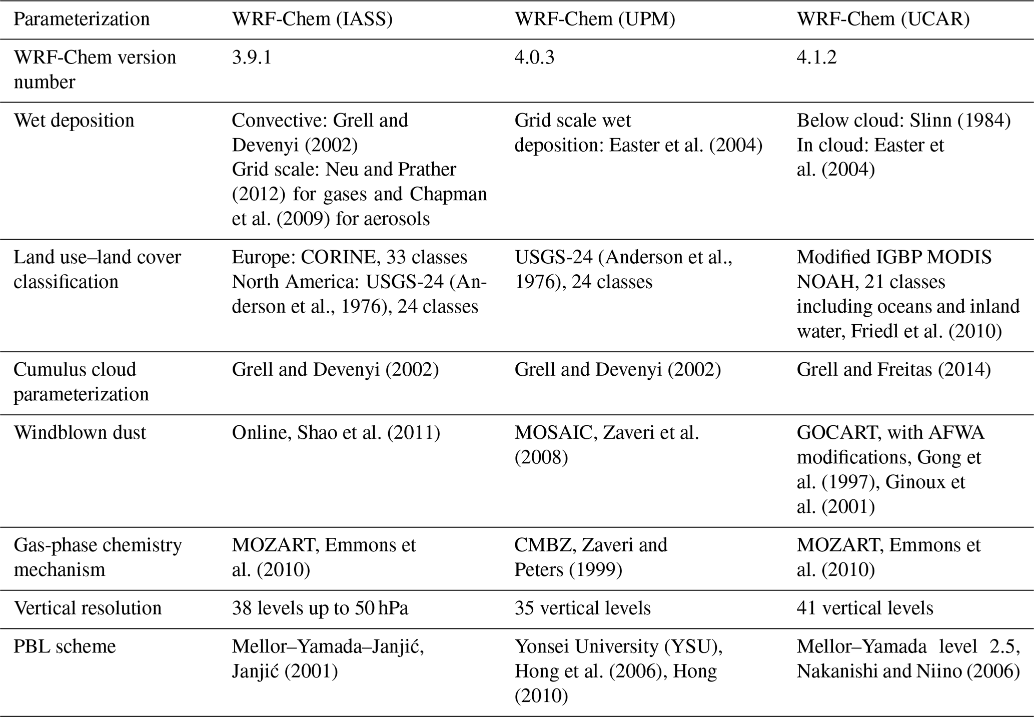
2.4.2 NA WRF-Chem (IASS), EU WRF-Chem (IASS); NA WRF-Chem (UPM), EU WRF-Chem (UPM); NA WRF-Chem (UCAR): WRF-Chem implementations

All three of these models made use of the WRF-Chem chemical transport modelling framework (Grell et al., 2005), employing a 12 km Lambert conformal conic projection (400 × 360 grid cells in the European domain, 480 × 290 grid cells in the North American domain), two-way coupling between air quality and meteorology, a sectional aerosol size distribution representation (four bins), aerosol microphysics and chemistry via the MOSAIC model (Zaveri et al., 2008), organic aerosol formation following Knote et al. (2014, 2015), cloud microphysics following Morrison et al. (2009), the Noah-Multiparameterization (Noah-MP) land surface model (Niu et al., 2011), the Rapid Radiative Transfer Model (RRTM) for radiative transfer calculations (Iacono et al., 2008), biogenic emissions using the MEGAN model (Guenther et al., 2006; Wiedinmyer et al., 2007), and the Fast-J algorithm for photolysis rate calculation (Chapman et al., 2009). All three code versions also make use of the Wesely (1989) parameterization for gas dry deposition and the Binkowski and Shankar (1995) approach for aerosol deposition. However, WRF-Chem has a large variety of configurations available for other model processes, allowing for the impact of those configurations on deposition results to be studied under AQMEII4. The differences between the model configurations are summarized in Table 1. It should also be noted that WRF-Chem is an online modelling framework; differences in the model parameterizations can influence the meteorological predictions through the aerosol direct and indirect effects, and consequently the meteorology generated by the implementations may also differ.

Not all of the WRF-Chem model implementations were able to report all of the information required to calculate exceedances: the WRF-Chem (IASS) implementation did not report all of the species contributing to S_dep and N_dep totals and also did not report several diagnostics requested under the AQMEII4 protocol. Consequently, the WRF-Chem (IASS) results were not included in ensemble deposition generation, and the model ensembles are referred to hereafter as “reduced ensembles”. Our analysis is therefore based on these reduced ensembles, though WRF-Chem (IASS) values for deposition totals have been provided when available in figures and tables for comparison purposes.

Table 1 AQMEII4 WRF-Chem configuration differences. PBL: planetary boundary layer.

2.4.3 LOTOS-EUROS (TNO): LOTOS-EUROS

LOTOS-EUROS (TNO) used in the AQMEII4 EU simulations is an open-source 3D chemistry transport model used extensively for air quality forecasts and scenarios for European domains (Timmermans et al., 2022; Manders et al., 2017). Gas dry-deposition fluxes made use of the approach based on Wesely (1989) (DEPosition of Acidifying Compounds, DEPAC; Van Zanten et al., 2010). Particle dry deposition was carried out using the approach of Zhang et al. (2001). Wet deposition followed the droplet saturation approach, and cloud chemistry with sulfate formation was dependent on cloud liquid water and droplet pH (Banzhaf et al., 2012). The dry deposition of ammonia makes use of a bidirectional flux approach (Wichink Kruit et al., 2012). Gas-phase chemistry was carried out using a modified form of the CBM-IV scheme (Gery et al., 1989; Whitten et al., 1980). N₂O₅ hydrolysis was included following Schaap et al. (2004), and inorganic thermodynamic particle chemistry was solved using the ISORROPIA II module (Fountoukis and Nenes, 2007). The model operated using 12 layers in the vertical in a hybrid coordinate system, with the near-surface layer having a thickness of ∼ 20 m and a model top of approximately 8 km. The simulations carried out here made use of a 20 × 20 km grid cell size over Europe. Driving meteorology for the model was from 3-hourly ECMWF short-term forecasts. Land use data for the model comes from the CORINE Land Cover 2000 database (EEA, 2000, 2007).

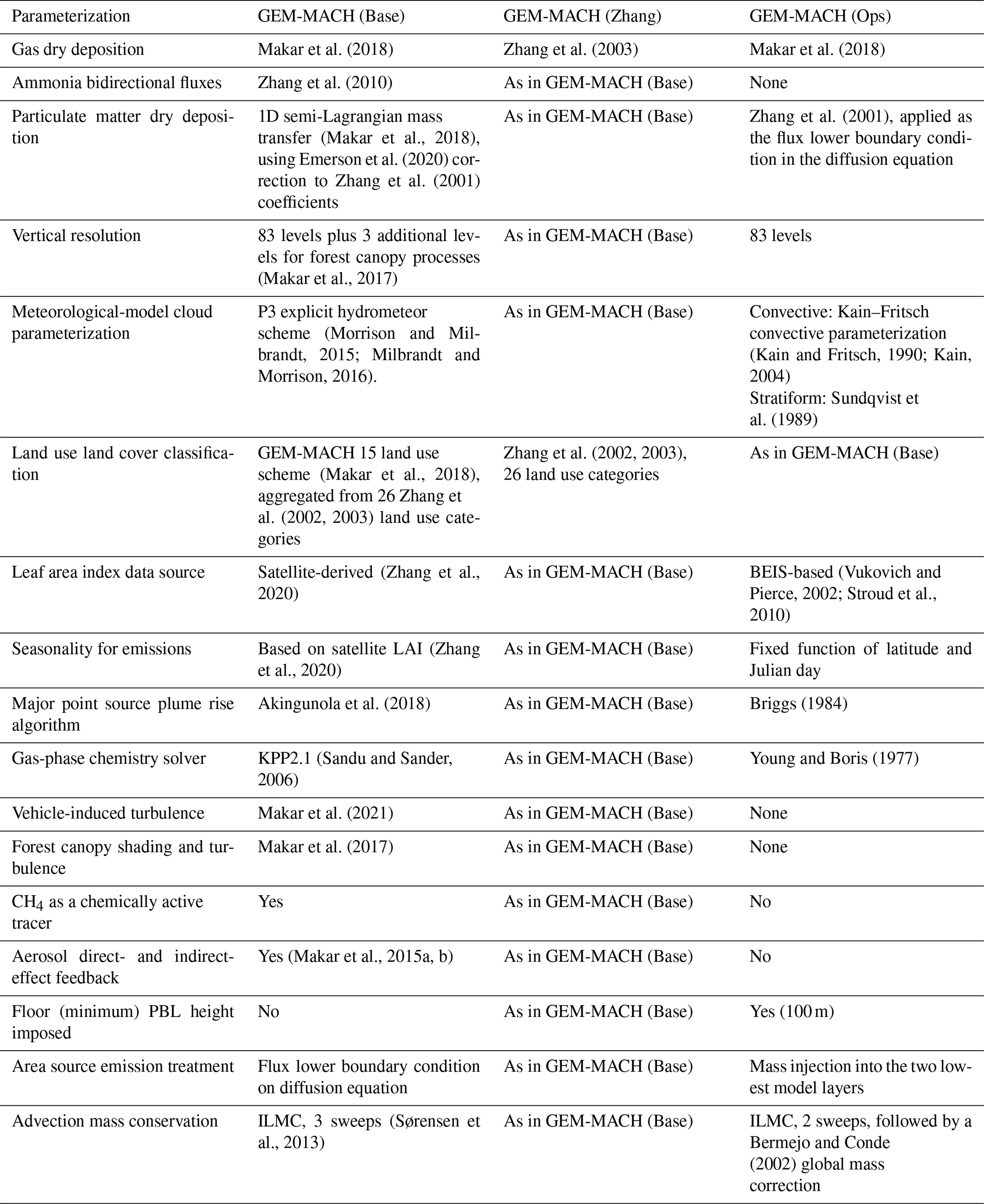
2.4.4 GEM-MACH (Base), GEM-MACH (Zhang), GEM-MACH (Ops): GEM-MACH

All three of these NA models are variations on the Environment and Climate Change Canada GEM-MACH model. The first two configurations (GEM-MACH (Base), GEM-MACH (Zhang)) are based on the “research” version of the model, which has more detailed physical parameterizations, whereas GEM-MACH (Ops) is based on the “operational forecast” configuration, where more simplified parameterizations have been employed in order to reduce processing time for operational air quality forecast simulations. Common elements across all three implementations include a horizontal grid cell size of 0.09° in a rotated latitude–longitude domain (∼ 10 km), 83 model levels, biogenic VOCs from BEIS versions 3.09 and 3.13 (Vukovich and Pierce, 2002; Stroud et al., 2010), a sectional aerosol size distribution (12 bins; Gong et al., 2003), the ADOM-II gas-phase mechanism (Stockwell and Lurmann, 1989), a modified Odum approach for secondary organic aerosol (SOA) formation (Stroud et al., 2018), and an inorganic aerosol chemistry module solving the thermodynamic equilibrium for the SO${}_{\mathrm{4}}^{\mathrm{2}-}$–NO${}_{\mathrm{3}}^{-}$–NH${}_{\mathrm{4}}^{+}$–H₂O system (Makar et al., 2003). The GEM-MACH implementations also all make use of the GEM weather forecast model v4.9.8 for driving meteorology (Côté et al., 1998; Girard et al., 2014), with the ISBA land surface scheme (Belair et al., 2003a, b) and the Canadian Climate Center for Modeling and Analysis Radiative transfer algorithm 2 (CCCMA Rad2; Li and Barker, 2005). As was the case for the WRF-Chem implementations described above, GEM-MACH has several optional process representations used in operational forecast versus research versions of the model; hence the relative importance of model configurations versus deposition parameterizations may be studied. The differences between the configurations are summarized in Table 2.

Collectively, the differences between GEM-MACH (Base) and GEM-MACH (Zhang) provide an estimate of the relative importance of the gas-phase deposition parameterization for simulation results, while comparisons between GEM-MACH (Base or Zhang) and GEM-MACH (Ops) show the relative impact of the combination of ammonia bidirectional fluxes and the suite of more complex physical parameterizations used in the former model configurations compared to the operational framework.

Table 2 AQMEII4 GEM-MACH configuration differences.

2.5 Bias-corrected critical load exceedance estimates

As will be discussed in Sect. 3.2, model results were evaluated using the available data for North America and Europe (see Sect. S7.0 in the Supplement for species contributing significantly to total S and N deposition). Critical load exceedances were calculated, making use of the total sulfur and total nitrogen deposition for each model in the ensemble, for 2009 and 2010 for Europe and for 2010 and 2016 for North America. In order to make a rough estimate of the impacts of model biases on the resulting exceedance estimates, a third set of exceedances were calculated for each model and each domain, for the year 2010 for Europe and 2016 for North America. For this last group, the ratio of the observed to model mean values at the observation station locations for individual species was used as scaling factors for the model annual deposition flux estimates prior to summation to total sulfur and total nitrogen deposition. Specifically, for North America, the ratio of the observed to measured mean concentrations of SO₂, NO₂, PM_2.5 sulfate, and PM_2.5 ammonium and Ammonia Monitoring Network (AMoN) NH₃ data were used to scale the corresponding dry flux variables, and the corresponding ratios for the wet deposition of sulfate, nitrate, and ammonium ions were used to scale the wet-deposition fluxes. Fewer observation data were available for Europe than North America: the ratios of observed to modelled SO₂ and NO₂ gas concentration mean values were used to scale the corresponding dry fluxes, and ratios of observed to modelled wet-deposition fluxes for sulfate, nitrate, and ammonium were used to scale the modelled wet-deposition fluxes.

We note that this approach makes simplifying assumptions. The corrections are inherently dependent on the assumption that the monitoring data are sufficiently representative of the model domain for the correction to be meaningful across the domain. While dry-deposition fluxes will be proportional to the concentrations in the lowest model layer, allowing an overall mean bias correction, we are also making the assumption that the bias ratios for PM_2.5 particulate matter will apply for larger particle sizes as well (note that size-resolved particulate fluxes were not reported under the AQMEII4 protocol). This form of bias correction is also the simplest possible means of model–measurement fusion; more complex methods appear in the literature. These methodologies for example may make use of a combination of observed wet and adjusted model dry deposition (Schwede and Lear, 2014), inverse distance weighting from observation stations (Rubin et al., 2023), and adjustment of modelled wet-deposition fluxes by the ratio of observed to simulated precipitation and by kriged observed wet deposition to model-predicted ratios (Zhang et al., 2019). An overview of model–measurement fusion approaches including advanced forms of data assimilation may be found in Fu et al. (2022). The methodology used here provides a first-order estimate of the impact of model biases with respect to observations of critical load exceedances.

3 Results

3.1 Critical load exceedances

3.1.1 Europe: acidification

Critical load exceedances for acidification for each of the four models for Europe (EU) are shown in Fig. 1 for 2010, Fig. S3 (Supplement) for 2009, and Fig. S9 (Supplement) for bias-corrected 2010. Figure 2 shows the reduced-ensemble values for 2009 and 2010 (a, b), the bias-corrected value for 2010 (c), and AQMEII4 common-domain total bar charts for all models and the reduced ensemble (d).

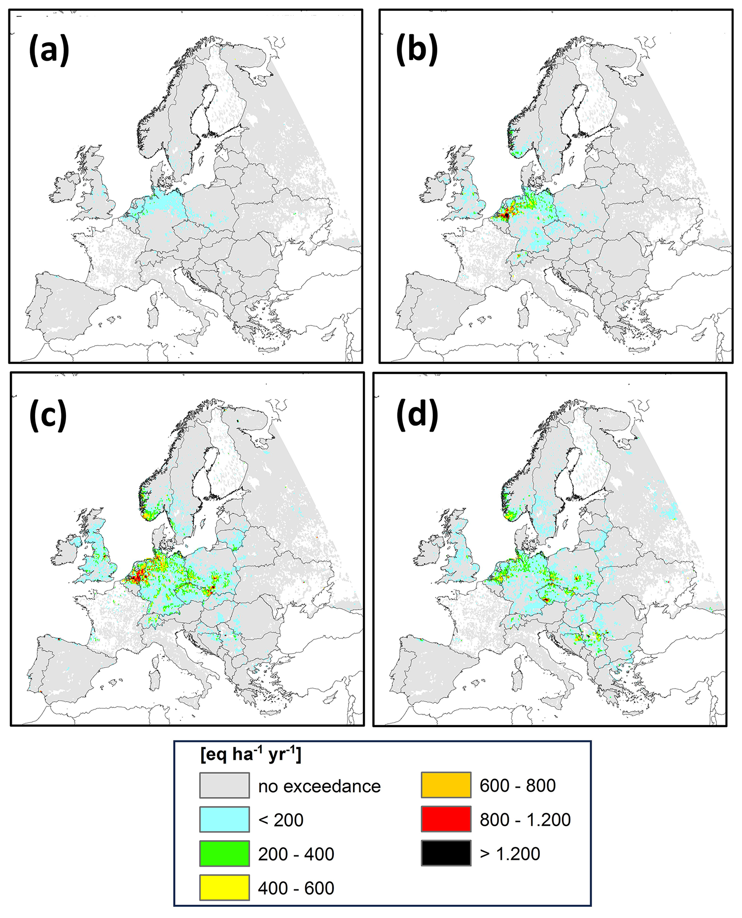
Figure 1 CLEs for acidity, EU AQMEII4 common domain, 2010, eq. ha⁻¹ yr⁻¹. (a) WRF-Chem (IASS), (b) LOTOS-EUROS (TNO), (c) WRF-Chem (UPM), (d) CMAQ (Hertfordshire). Grey areas indicate regions for which critical load data are available but are not in exceedance of critical loads. Coloured areas indicate exceedance regions.

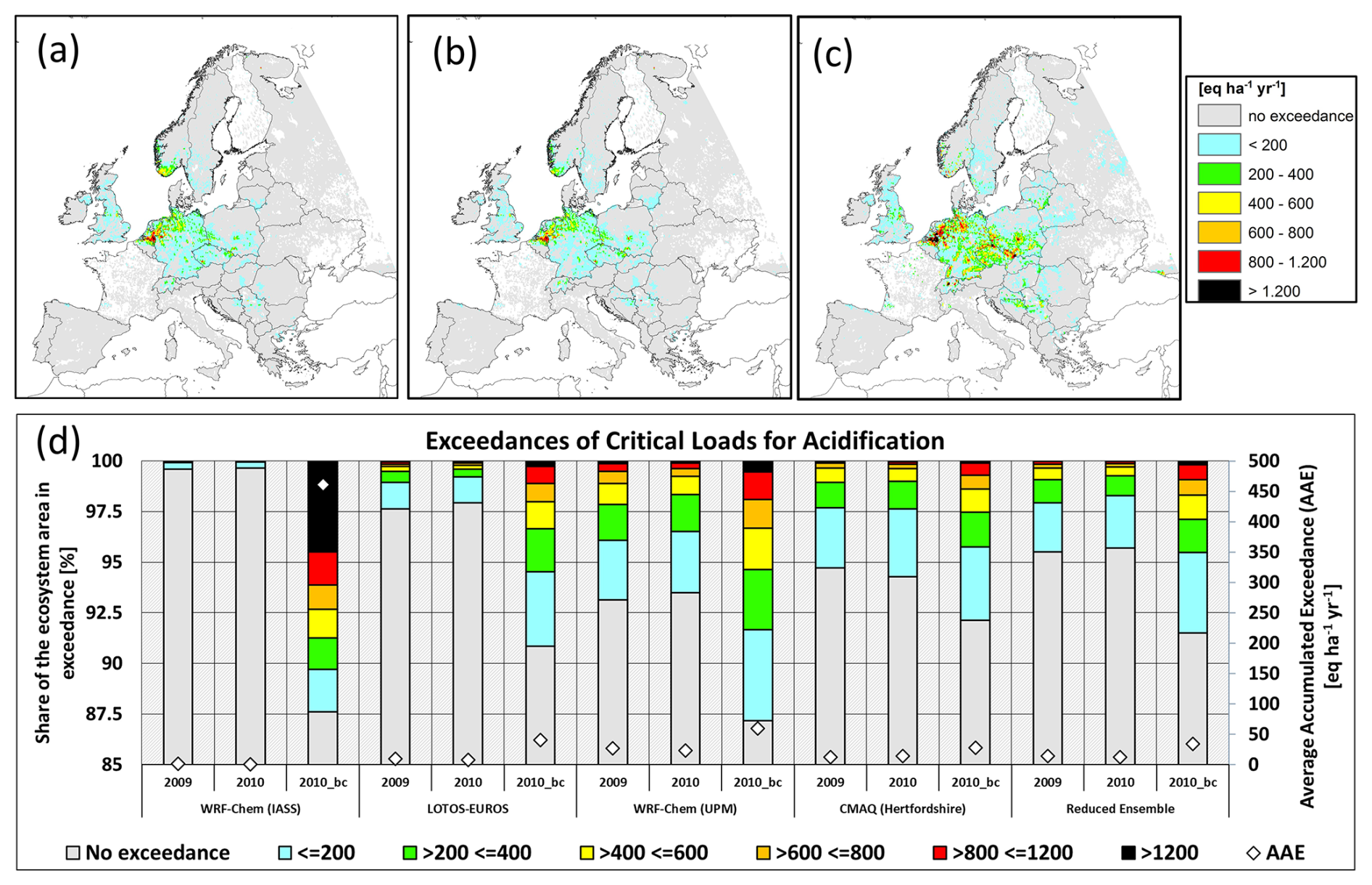
Figure 2 Summary CLEs for acidity, EU AQMEII4 common domain, eq. ha⁻¹ yr⁻¹. (a, b) Spatial distribution of CLEs for the reduced ensemble for the years 2009 and 2010, respectively. (c) Spatial distribution of CLE for the bias-corrected reduced ensemble for the year 2010. (d) Percentage of ecosystems for which CL data are available that are in exceedance by model and year (left axis and colour bar) and average accumulated exceedance (eq. ha⁻¹ yr⁻¹) (right axis and black diamonds). Reduced-ensemble CLEs for the years 2009, 2010, and bias-corrected 2010 (2010_bc) appear on the right side of panel (d).

The EU exceedances for acidity are similar between the 2 years (compare Figs. 1 and S3 and reduced-ensemble values for each year in Fig. 2). However, differences between models within a given year are larger (especially in an absolute sense; WRF-Chem (IASS) of <0.4 % in exceedance, WRF-Chem (UPM) of ∼ 6.5 %). Low WRF-Chem (IASS) exceedance levels are in part due to unreported deposition data (see Sect. 2.2.2); the reduced-ensemble maps in Fig. 2 show the ensemble average for LOTOS-EUROS (TNO), WRF-Chem (UPM), and CMAQ (Hertfordshire). The EU reduced ensemble shows the greatest extent of exceedance in the Netherlands along the Netherlands–Belgium border, northwestern Germany, southern Norway, and along the border between Poland and Germany (Fig. 2a, b). Individual models in Fig. 1 show additional acidity “hotspots” that may appear in one model and not in another (e.g. LOTOS-EUROS (TNO): near Lucerne and Bonn; WRF-Chem (UPM): westernmost Switzerland, south-central Germany, and Belgrade; CMAQ (Hertfordshire): southwestern Switzerland, south-central Germany, and southwestern Romania). Bias correction for the reduced ensemble for the 2010 data resulted in substantial increases in predicted exceedances (compare the last two columns of Fig. 2d and compare Fig. 1 to Fig. S9). However, we note that the European data did not include speciated particulate matter, and hence bias correction was not possible for part of the sulfur budget; much smaller impacts were noted for bias correction in North America where particulate sulfate data were available.

The percent area of the EU acidification CLE over the region for which CL data were available, for the reduced ensemble, was 4.48 % (range of 2.37 % to 6.85 %) in 2009 and 4.32 % (2.06 to 6.52 %) in 2010. Average reduced-ensemble accumulated exceedance for EU acidity was 13.8 (9.7 to 27.1) eq. ha⁻¹ yr⁻¹ in 2009 and 12.6 (7.8 to 23.7) eq. ha⁻¹ yr⁻¹ in 2010. The quoted range is from the highest and lowest members in the three-member reduced ensemble.

3.1.2 Europe: eutrophication

Critical load exceedances for eutrophication for each of the four EU models are shown in Fig. 3 for 2010, in Fig. S4 (Supplement) for 2009, and with bias-corrected deposition fields for 2010 in Fig. S10 (Supplement). Figure 4 shows the reduced-ensemble values for 2009 and 2010 (a, b), the bias-corrected values for 2010 (c), and the AQMEII4 common-domain summaries for all models and the ensembles (d).

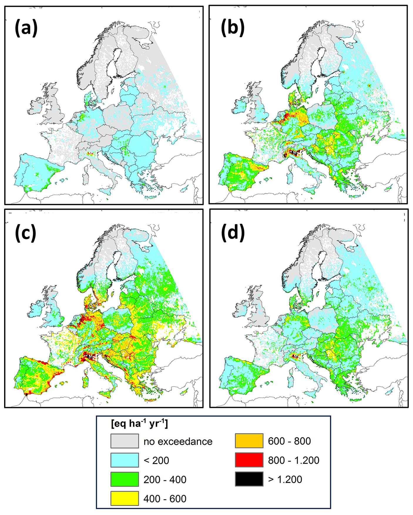
Figure 3 CLEs for eutrophication, EU AQMEII4 common domain, 2010, eq. ha⁻¹ yr⁻¹. (a) WRF-Chem (IASS), (b) LOTOS-EUROS (TNO), (c) WRF-Chem (UPM), (d) CMAQ (Hertfordshire). Grey areas indicate regions for which critical load data are available but are not in exceedance of critical loads. Coloured areas indicate exceedance regions.

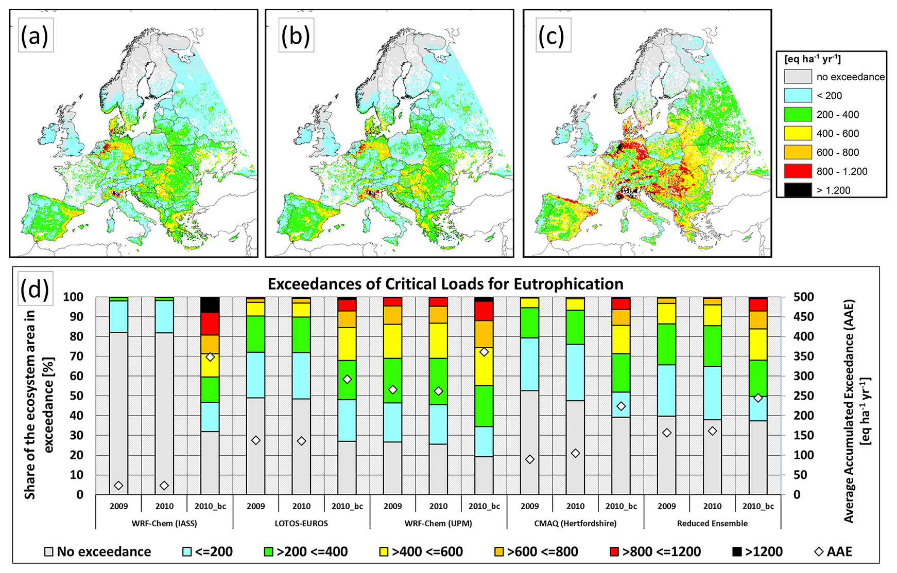
Figure 4 Summary CLEs for eutrophication, EU AQMEII4 common domain, eq. ha⁻¹ yr⁻¹. (a, b) Spatial distribution of CLEs for the reduced ensemble for the years 2009 and 2010, respectively. (c) Spatial distributions of CLEs for the bias-corrected reduced ensemble for 2010. (d) Percentage of ecosystems for which CL data are available that are in exceedance by model and year (left axis and colour bar) and average accumulated exceedance (eq. ha⁻¹ yr⁻¹) (right axis and black diamonds). Reduced-ensemble CLEs for the years 2009, 2010, and bias-corrected 2010 (2010_bc) appear on the right side of panel (d).

As for EU acidity CLEs, the eutrophication CLEs are very similar between the 2 model years (compare Figs. 3 and S4 and the values for each year in Fig. 4). The spatial distribution of the greatest levels of exceedance also varies more strongly between models. All members in the three-member reduced ensemble identify the Po River valley as reaching the greatest level of exceedance, but LOTOS-EUROS (TNO) also shows high levels of exceedance from Benelux to northern Germany and in the Barcelona area, while WRF-Chem (UPM) shows high levels of exceedance of >800 eq. ha⁻¹ yr⁻¹ in multiple hotspots throughout the region. The relative impact of bias correction was smaller than for acidification in terms of the total area in exceedance, but the magnitude of exceedances increased significantly (e.g. larger proportion of red to black areas in Fig. 4c than Fig. 4b, comparing the last two columns of Fig. 4d and comparing Fig. 4 to Fig. S10). Again, the higher levels of exceedance predicted for Europe may reflect the impact of the lack of particulate sulfate and particulate nitrate data for bias correction purposes.

The percentage of the area in exceedance for eutrophication is much higher than that of acidification (reduced-ensemble CLE of 60.2 % (47.3 % to 73.3 %) in 2009 and 62.2 % (51.2 % to 74.4 %) in 2010). The average accumulated exceedance was 156.9 (89.4 % to 265.5) eq. ha⁻¹ yr⁻¹ in 2009 and 161.4 (109.4 to 261.8) eq. ha⁻¹ yr⁻¹ in 2010 (in Fig. 4 the range is from the lowest and highest members in the three-member reduced ensemble).

3.1.3 North America: forest-ecosystem simple mass balance critical load

Critical load exceedances with respect to the forest soil acidity for North America (NA) for the years 2016 and 2010 are shown in Figs. 5 and S5, respectively; the bias-corrected 2016 maps are in Fig. S11, and the reduced-ensemble maps for both years, as well as the domain summaries, including bias-corrected values for 2016, are shown in Fig. 6.

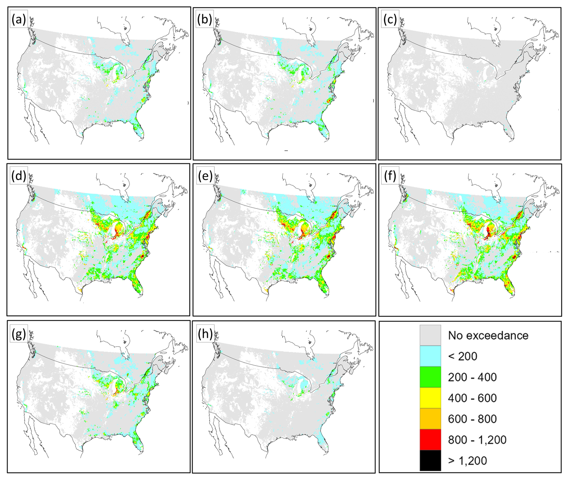
Figure 5 CLEs for forest soil acidification, NA AQMEII4 common domain, 2016, eq. ha⁻¹ yr⁻¹. (a) CMAQ-M3Dry, (b) CMAQ-STAGE, (c) WRF-Chem (IASS), (d) GEM-MACH (Base), (e) GEM-MACH (Zhang), (f) GEM-MACH (Ops), (g) WRF-Chem (UPM), (h) WRF-Chem (UCAR). Grey areas indicate regions for which critical load data are available but are not in exceedance of critical loads. Coloured areas indicate exceedance regions.

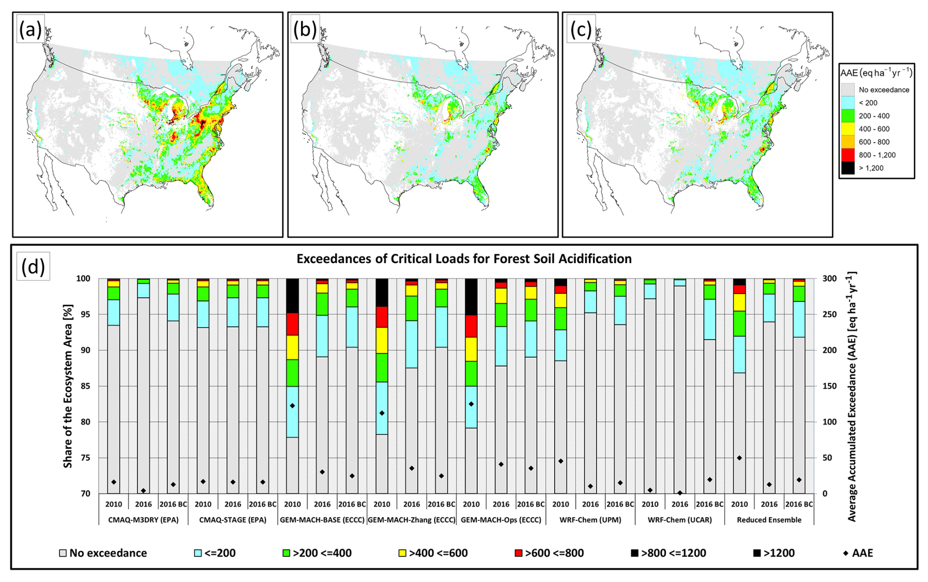
Figure 6 Summary CLEs for forest soil acidification, NA AQMEII4 common domain, eq. ha⁻¹ yr⁻¹. (a, b) Spatial distribution of CLEs for the reduced ensemble for the years 2010 and 2016, respectively. (c) Spatial distribution of CLEs for the reduced ensemble for the year 2016. (d) Percentage of ecosystems for which CL data are available that are in exceedance by model and year (left axis and colour bar) and average accumulated exceedance (eq. ha⁻¹ yr⁻¹) (right axis and black diamonds). Reduced-ensemble CLEs for the years 2010, 2016, and bias-corrected 2016 (2016 BC) appear on the right side of panel (d).

Unlike the EU domain comparison, the NA CLEs depicted in Fig. 5 show a large difference in the extent of regions in exceedance for the different models. While all models with the exception of WRF-Chem (IASS) identified the regions to the south and west of the Great Lakes, the US East Coast, and Florida as being in exceedance, the magnitude of the exceedances varied greatly between the models, with the GEM-MACH models (Fig. 5d–f) showing large regions with exceedances above 800 eq. ha⁻¹ yr⁻¹, followed by, in descending order, WRF-Chem (UPM), CMAQ-M3Dry, CMAQ-STAGE, WRF-Chem (UCAR), and WRF-Chem (IASS).

The summary reduced-ensemble CLE values (Fig. 6) show the improvement in CLEs between the years 2010 and 2016, which occurred in response to the legislated reduction in SO₂ emissions during this time period. The summary chart (Fig. 6c) however shows that the magnitude of the response to the SO₂ reduction was model dependent: the change between 2010 and 2016 was the greatest for GEM-MACH (Base) in an absolute sense and the greatest for WRF-Chem (UCAR) in a relative sense. Similarly, the average accumulated exceedance (right-hand vertical axis and black diamonds, Fig. 6c) showed decreases in exceedance between 2010 and 2016 for all models, but the extent of these decreases differed, with WRF-Chem (UCAR) showing the smallest decrease in AAE from 2010 to 2016, followed in increasing order of the magnitude of change by CMAQ-STAGE, CMAQ-M3Dry WRF-Chem (UPM), GEM-MACH (Ops), GEM-MACH (Base), and GEM-MACH (Zhang).

The effect of bias correction was less pronounced than in Europe and, in general, reduced the variability between model results. Note that unlike the European case, North American observation data used for bias correction included corrections for particulate sulfate air concentrations, allowing for a greater degree of closure for the sulfur mass deposited. Comparing Figs. 5 and S11 it can be seen that the bias correction has increased exceedances for the CMAQ and WRF-Chem simulations and decreased exceedances for the GEM-MACH simulations, reducing the variability between the models. The extent to which model-to-model variability has been reduced following bias correction is also apparent in Fig. 6d (bias correction exceedance bars are closer in size across models compared to before bias correction). The net result is bias correction being a slight increase in the area of exceedance in the reduced ensemble, comparing the two right-hand bars of Fig. 6d.

The percentage of the NA forested area in exceedance for acidification for the reduced ensemble was 13.2 % (2.8 % to 22.2 %) in 2010 and 6.1 % (1.0 % to 12.9 %) in 2016. The ensemble thus shows a considerable improvement in exceedances with respect to acidification between the 2 years.

3.1.4 North America: aquatic-ecosystem critical-load exceedances with respect to acidity)

Exceedances with respect to the North American aquatic-ecosystem CL dataset for the years 2016 and 2010 are shown in Figs. 7 and S6, respectively; the bias-corrected maps for each model for 2016 are in Fig. S12; and the reduced-ensemble maps for both years and domain summaries, including bias correction, are shown in Fig. 8.

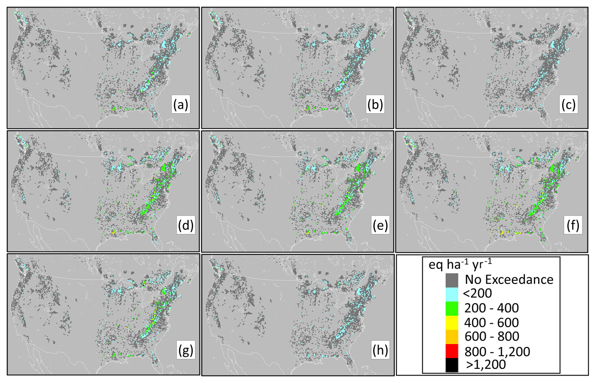
Figure 7 CLEs for aquatic ecosystems, NA AQMEII4 common domain, 2016, eq. ha⁻¹ yr⁻¹. Panels arranged by model as in Fig. 6; individual sites are shown as pixels. Dark-grey pixels indicate regions for which critical load data were available but were not in exceedance of critical loads. Coloured areas indicate exceedance regions; overplotting in precedence by the extent of exceedance was carried out for overlapping pixels. Areas of no CL data are shown in lighter grey.

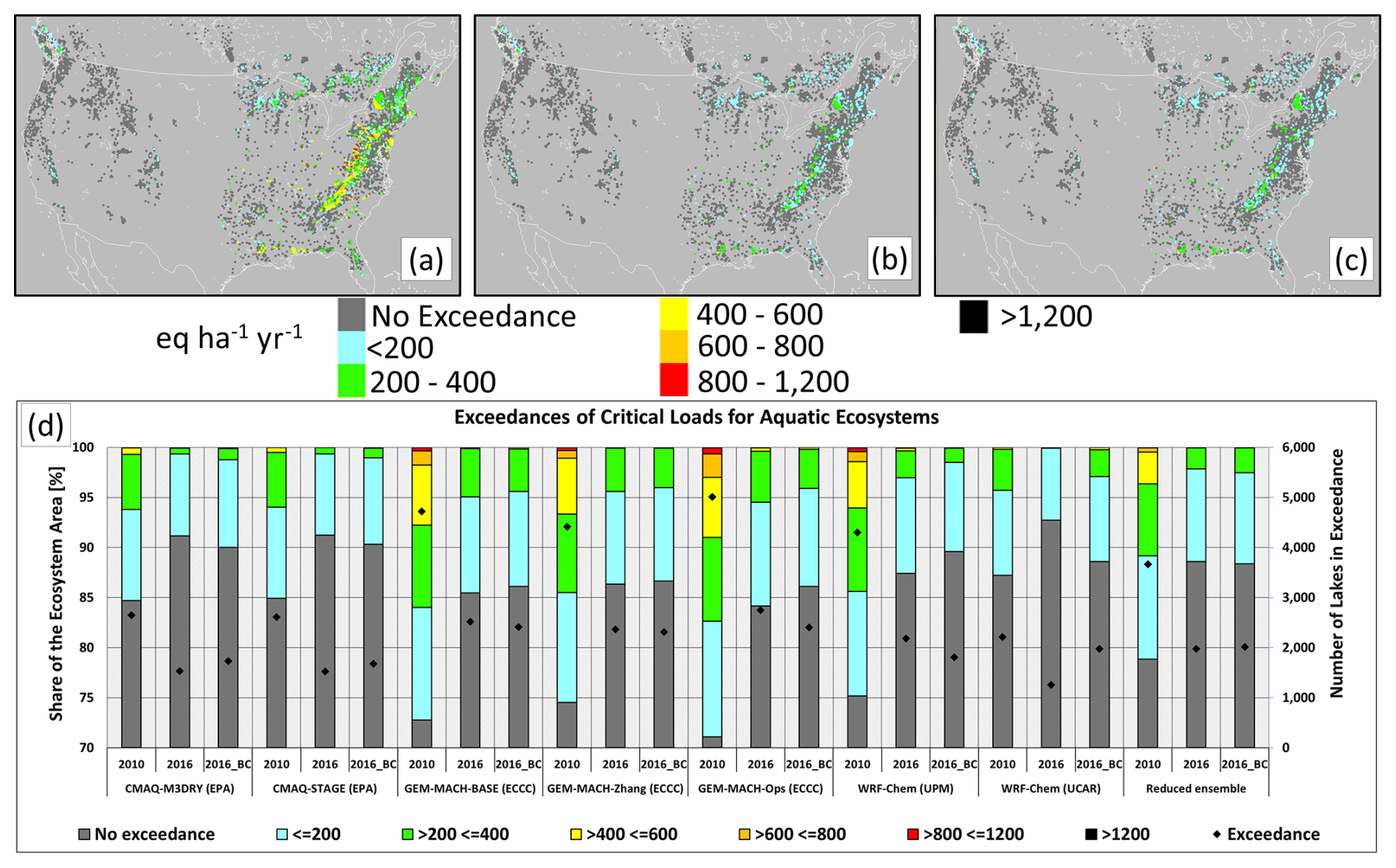
Figure 8 Summary CLEs for aquatic ecosystems, NA AQMEII4 common domain. (a, b) Spatial distribution of CLEs for the reduced ensemble for the years 2010 and 2016, respectively. (c) Spatial distribution of CLEs for the bias-corrected reduced ensemble for the year 2016. (d) Percentage of lakes for which CL data are available that are in exceedance by model and year (left axis and colour bar) and number of lakes in exceedance (right axis and black diamonds). Reduced-ensemble CLEs for the years 2010, 2016, and bias-corrected 2016 (2016_BC) appear on the right side of panel (d).

Comparison of Figs. 5 and 7 shows a similarity in the CLE response of the individual models between forest soil and aquatic ecosystems, with the GEM-MACH models predicting the highest number and magnitude of exceedances, followed by WRF-Chem (UPM), WRF-Chem (UCAR), and the two CMAQ implementations. Figure 8a and b show the expected decrease in the reduced-ensemble CLE between 2010 and 2016, as well as the higher levels of exceedance associated with the GEM-MACH and WRF-CHEM (UPM) models, followed in descending order by the two CMAQ implementations and WRF-CHEM (UCAR) (Fig. 8c).

The impact of bias correction on the North American aquatic-ecosystem critical load exceedances was relatively minimal for the models included in the reduced ensemble: differences between Figs. 7 and S12 are difficult to distinguish, and Fig. 8d shows slight increases in the exceedances for CMAQ and WRF-Chem simulations, slight increases in GEM-MACH simulations, and a very small change in the reduced-ensemble levels of exceedance.

The percentage of the NA aquatic ecosystems in exceedance for the reduced ensemble was 21.2 % (12.8 % to 28.9 %) in 2010 and 11.4 % (7.3 % to 15.8 %) in 2016. The reduced ensemble thus shows a considerable improvement in exceedances with respect to the exceedance of aquatic critical loads between the 2 years, again by almost a factor of 2.

3.1.5 US N deposition to lichen

Exceedances with respect to the US CL of N for a 20 % decline in the sensitive-epiphytic-lichen species richness (221 eq. N ha⁻¹ yr⁻¹) dataset for the years 2016 and 2010 are shown in Figs. 9 and S7, respectively; bias-corrected 2016 values are in Fig. S13; and the reduced-ensemble maps for both years and domain summaries, including bias-corrected 2016 values, are shown in Fig. 10.

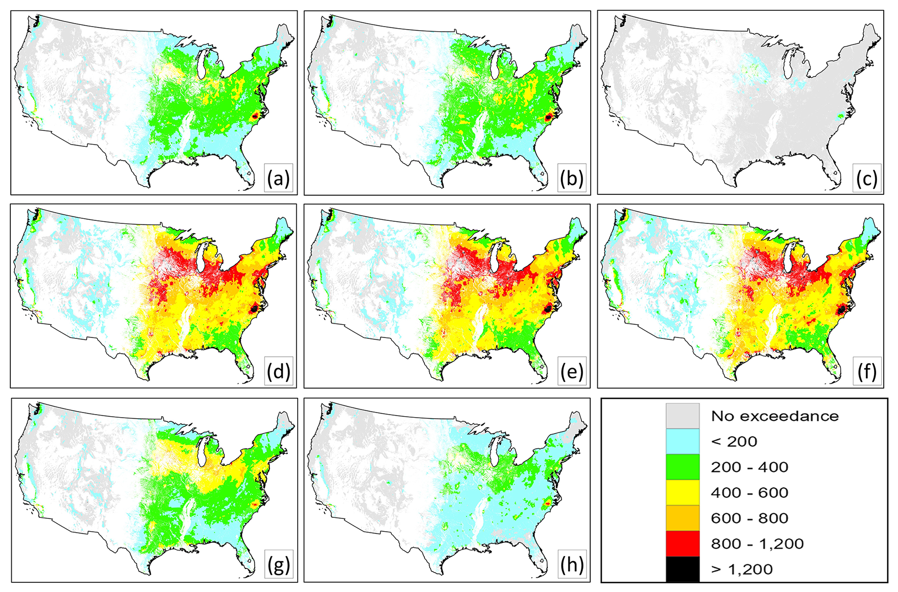
Figure 9 CLEs for sensitive-epiphytic-lichen species, NA AQMEII4 common domain, 2016, eq. ha⁻¹ yr⁻¹. Panels arranged by model as in Fig. 6. Light-grey areas indicate regions for which critical load data were available but were not in exceedance of critical loads. Coloured areas indicate exceedance regions.

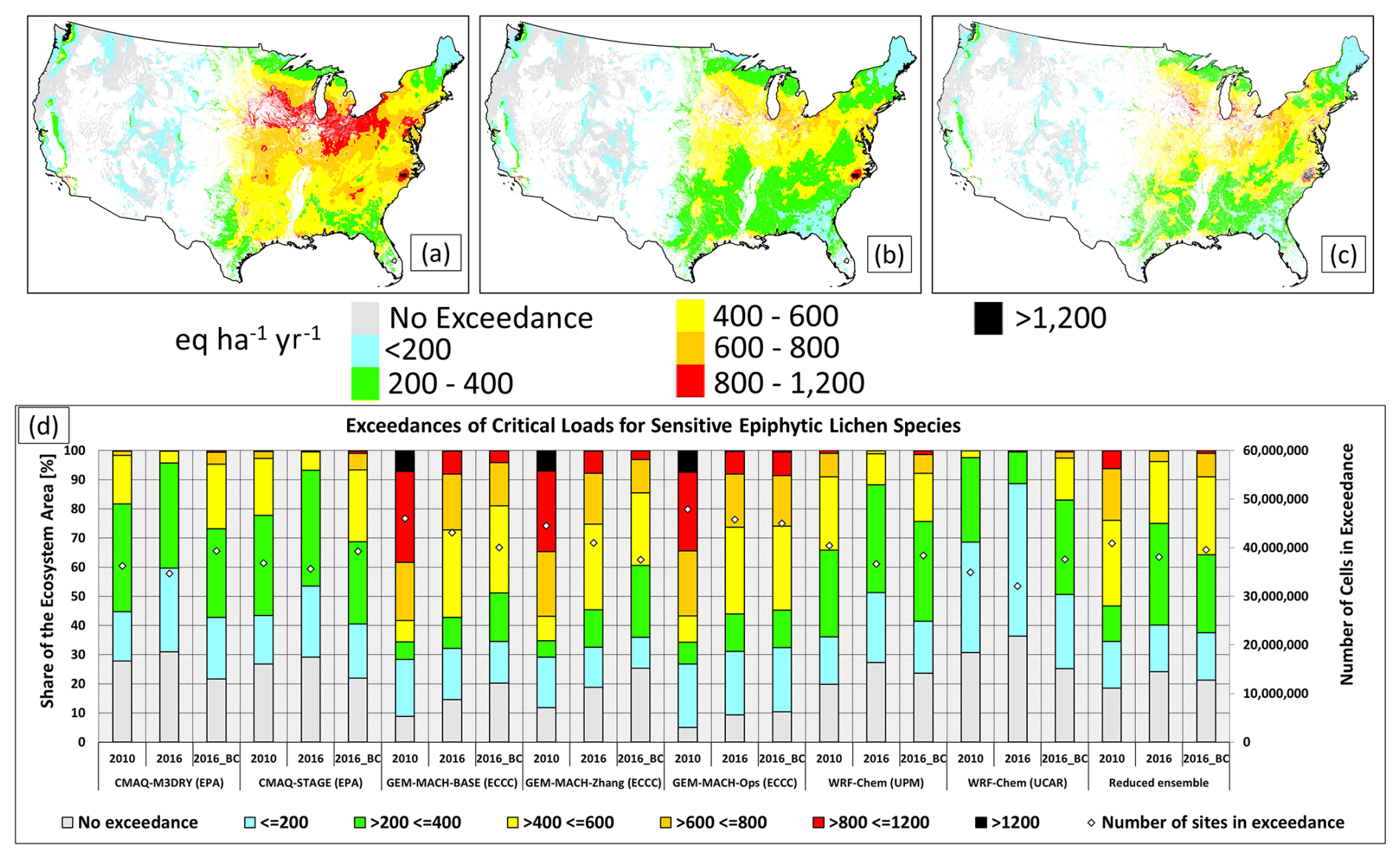
Figure 10 Summary CLEs, sensitive-epiphytic-lichen species, NA AQMEII4 common domain, eq. ha⁻¹ yr⁻¹. (a, b) Spatial distribution of CLEs for the reduced ensemble for the years 2010 and 2016, respectively. (c) Spatial distribution of CLEs for the bias-corrected reduced ensemble for the year 2016. (d) Percentage of sensitive-epiphytic-lichen ecosystems for which CL data are available that are also are in exceedance by model and year (left axis and colour bar) and number of sites in exceedance (right axis and white diamonds). Reduced-ensemble CLEs for the years 2010, 2016, and bias-corrected 2016 (2016_BC) appear on the right side of panel (d).

The overall pattern of exceedances and their magnitude across models (Fig. 9) is similar to that of the forest soil exceedances (Fig. 5), with the largest magnitudes in the northeastern continental USA and in North Carolina, though the lichen exceedances are more continuous across the region than for forest soil water acidity-impacted ecosystems. GEM-MACH (Base), GEM-MACH (Zhang), and GEM-MACH (Ops) have maximum exceedances usually between 800 and 1200 eq. ha⁻¹ yr⁻¹, and the exceedances predicted by other models are less than 800 eq. ha⁻¹ yr⁻¹, aside from a North Carolina exceedance hotspot which is predicted by all models. The overall reduced-ensemble magnitude of exceedances decreased significantly between 2010 and 2016 (Fig. 10a, b; fewer black and red regions in the more recent year). The reduced-ensemble total area in exceedance has decreased slightly (columns labelled “Reduced ensemble” in Fig. 10d). All models show a decreasing levels of exceedance between the 2 years and a slightly decreasing total area of exceedance. The magnitude of exceedance differs significantly between the models, with the highest-magnitude exceedances predicted by the GEM-MACH group of models, followed by WRF-Chem (UPM).

Bias correction values varied between the models, with CMAQ exceedances increasing slightly, GEM-MACH exceedances decreasing slightly, WRF-Chem exceedances increasing, and a slight increase in the overall extent and magnitude of the reduced-ensemble exceedances in the last two columns of Fig. 10d. The similarity in the spatial distribution of exceedances is greater across models following bias correction (compare Fig. 9 with Fig. S13 in the Supplement).

The percentage of the NA sensitive-epiphytic-lichen ecosystems in exceedance for the reduced ensemble was 81.5 % (69.3 % to 95.0 %) in 2010 and 75.8 % (63.7 % to 90.7 %) in 2016.

3.1.6 US N deposition to herbaceous plants

Exceedances with respect to the US CL of N for a decline in the herbaceous-species richness (436 to 1693 eq. N ha⁻¹ yr⁻¹) dataset for the years 2016 and 2010 are shown in Figs. 11 and S8, respectively; bias-corrected exceedances for 2016 appear in Fig. S14 (Supplement); and the reduced-ensemble maps for both years and domain summaries, including bias correction for 2016, are shown in Fig. 12.

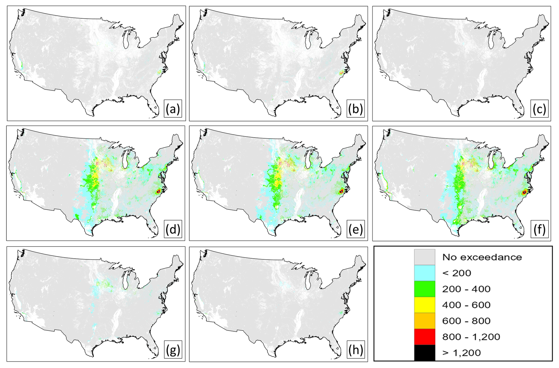
Figure 11 CLEs for a decline in herbaceous-species community richness, NA common domain, 2016, eq. ha⁻¹ yr⁻¹. Panels arranged by model as in Fig. 6. Light-grey areas indicate regions for which critical load data were available but were not in exceedance of critical loads. Coloured areas indicate exceedance regions.

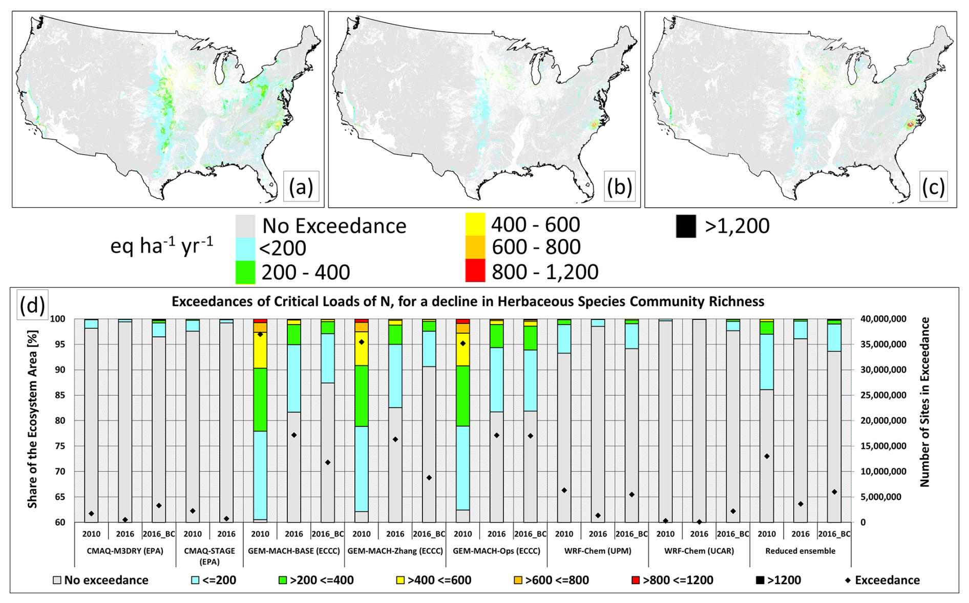
Figure 12 Summary CLEs for a decline in herbaceous-species community richness, NA AQMEII4 common domain, eq. ha⁻¹ yr⁻¹. (a, b) Spatial distribution of CLEs for the reduced ensemble for the years 2010 and 2016, respectively. (c) Spatial distribution of CLEs for the bias-corrected reduced ensemble for the year 2016. (d) Percentage of herbaceous-species communities for which CL data are available that are also are in exceedance by model and year (left axis and colour bar) and number of sites in exceedance (right axis and white diamonds). Reduced-ensemble CLEs for the years 2010, 2016, and bias-corrected 2016 (2016 BC) appear on the right side of panel (d).

The spatial distribution of the regions of the highest exceedance shares some common features with that of sensitive epiphytic lichen (compare Fig. 11 with Fig. 9), such as maximum exceedances in the northeastern USA, in North Carolina, and extending along a region north of Texas. However, both the magnitude and extent of exceedance is much more varied for herbaceous-species richness than for lichen species richness, with the GEM-MACH suite of models (Figs. 11d–f and 12d) predicting the highest exceedance levels and up to 18.4 % of the area in exceedance in 2016, with the CMAQ implementations varying between 0.6 % and 0.8 % and WRF-Chem (UCAR) predicting 0.1 %.

The impacts of bias correction may be more easily distinguished for herbaceous-species richness critical load exceedances compared to some of the other exceedance estimates (compare Figs. 11 and S14), with the CMAQ and WRF-Chem exceedances increasing and the GEM-MACH exceedances decreasing. The overall impact was a slight increase in the area and extent of the ensemble average exceedance (Fig. 12d).

The percentage of the NA herbaceous-plant ecosystems in exceedance for the reduced ensemble was 13.9 % (0.4 % to 39.5 %) in 2010 and 3.9 % (0.1 % to 18.4 %) in 2016, with the higher exceedance levels in the range resulting from the GEM-MACH suite of models. Reduced-ensemble herbaceous-species richness exceedances have decreased considerably between the 2 years in all models.

3.1.7 Critical load exceedances: key results

The percent exceedance for the reduced ensemble and ranges from the reduced ensembles for the ecosystems examined here are summarized in Table 3. The values suggest acidification in Europe will happen over a smaller region than eutrophication at 2009–2010 emission levels, with a slight decrease in acidification and a slight increase in eutrophication between the 2 years. About 60 % of EU ecosystems would be subject to eutrophication at some point in the future at 2009–2010 emission levels. One striking difference between the different model estimates of CLE is in the magnitude of exceedances (as opposed to the total area in exceedance). WRF-Chem (UPM) for example in Figs. 1 and 3 predicts more severe levels of exceedance across Europe than the other models. The North American results suggest that reductions in SO₂ and NO_x emissions between 2010 and 2016 resulted in a substantial reduction in the number of forest soil and aquatic-ecosystem acidification exceedances (by nearly a factor of 2). The impacts of nitrogen deposition on herbaceous species also improved (by nearly a factor of 3), while impacts of nitrogen deposition on sensitive lichen had a more modest improvement (from 81.5 % to 75.8 % in exceedance). The magnitude and spatial extent of these eutrophication exceedances were highly dependent on the model and on the variations in the representation of sub-processes within each model, used for predictions. Understanding the large range of model predictions is one of the main aims of the current work. The next section discusses the underlying causes driving the model-to-model differences, using the AQMEII4 deposition diagnostics.

Table 3 Summary of reduced-ensemble percent exceedance mean values and their range in the EU and NA domains, along with total S deposition and total N deposition predicted by the ensemble. All models used the same starting inventories for emissions.

3.2 Analysis of model deposition predictions

3.2.1 Causes of S deposition variability in North American domain simulations

The AQMEII4 common-grid average and percent contribution of each depositing species to total S deposition in 2016 are given in Table 4. The averages and standard deviation for the reduced ensemble show that wet deposition of the sum of the sulfate and bisulfite ions (SO${}_{\mathrm{4}}^{(\mathrm{2}-)}$ and HSO${}_{\mathrm{3}}^{(-)}$) contributes more to total S deposition than particulate sulfate dry deposition, which is in turn contributes more than SO₂(g) (gas) dry deposition. However, the model-to-model variability is also large, particularly for the contribution of particulate sulfate, which varies by nearly 2 orders of magnitude between GEM-MACH (Base), GEM-MACH (Zhang), and GEM-MACH (Ops) and WRF-Chem (UPM). The contributions to the average reduced-ensemble total S deposition are 62.0 ± 19.3, 44.8 ± 39.0, and 28.8 ± 9.9 eq. ha⁻¹ yr⁻¹ for wet, particle dry, and gas dry deposition, respectively (± ranges in Table 4 are the standard deviation of the component). The greatest cause of model variability in absolute total deposition is associated with the contribution of particulate sulfate dry deposition, followed by sulfur wet deposition and then gaseous SO₂ dry deposition.

Table 4 Average S deposition contributions in the NA AQMEII4 common-grid area (eq. ha⁻¹ yr⁻¹) and percent contribution to average total S deposition, 2016. n/d: no data submitted or insufficient data to calculate a percentage.

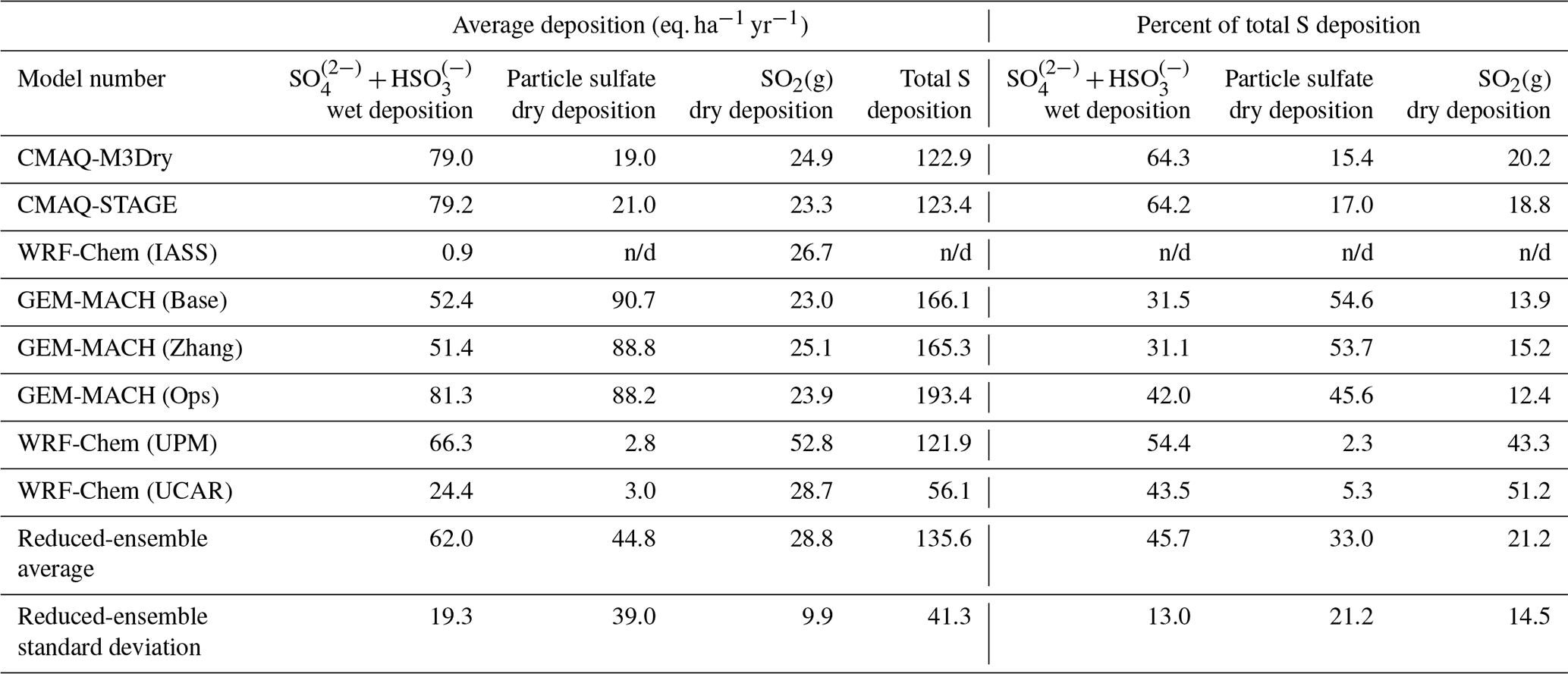
The spatial distributions of the two largest components of the total S deposition variability (wet S and dry particle S) are shown in Fig. 13. The WRF-Chem (IASS) values did not represent the expected sources of S deposition over the continent, and some deposition fields such as the total particulate sulfate dry deposition were not submitted. The S wet-deposition maps are qualitatively similar between the other models (note that the colour scale is logarithmic), with WRF-Chem (UCAR) having the lowest values (Fig. 13a). As shown in Table 4, the greatest degree of variability between the different modelling platforms is in the particle deposition fluxes (Fig. 13b). This variability extends over orders of magnitude. WRF-Chem (UPM) and WRF-Chem (UCAR) predict the lowest deposition fluxes of dry particulate sulfate over both land and ocean. CMAQ-STAGE and CMAQ-M3Dry predict higher values over parts of the ocean but relatively low values over land. GEM-MACH (Base), GEM-MACH (Zhang), and GEM-MACH (Ops) have the highest particulate sulfate dry-deposition fluxes, roughly equivalent to the wet-deposition fluxes.

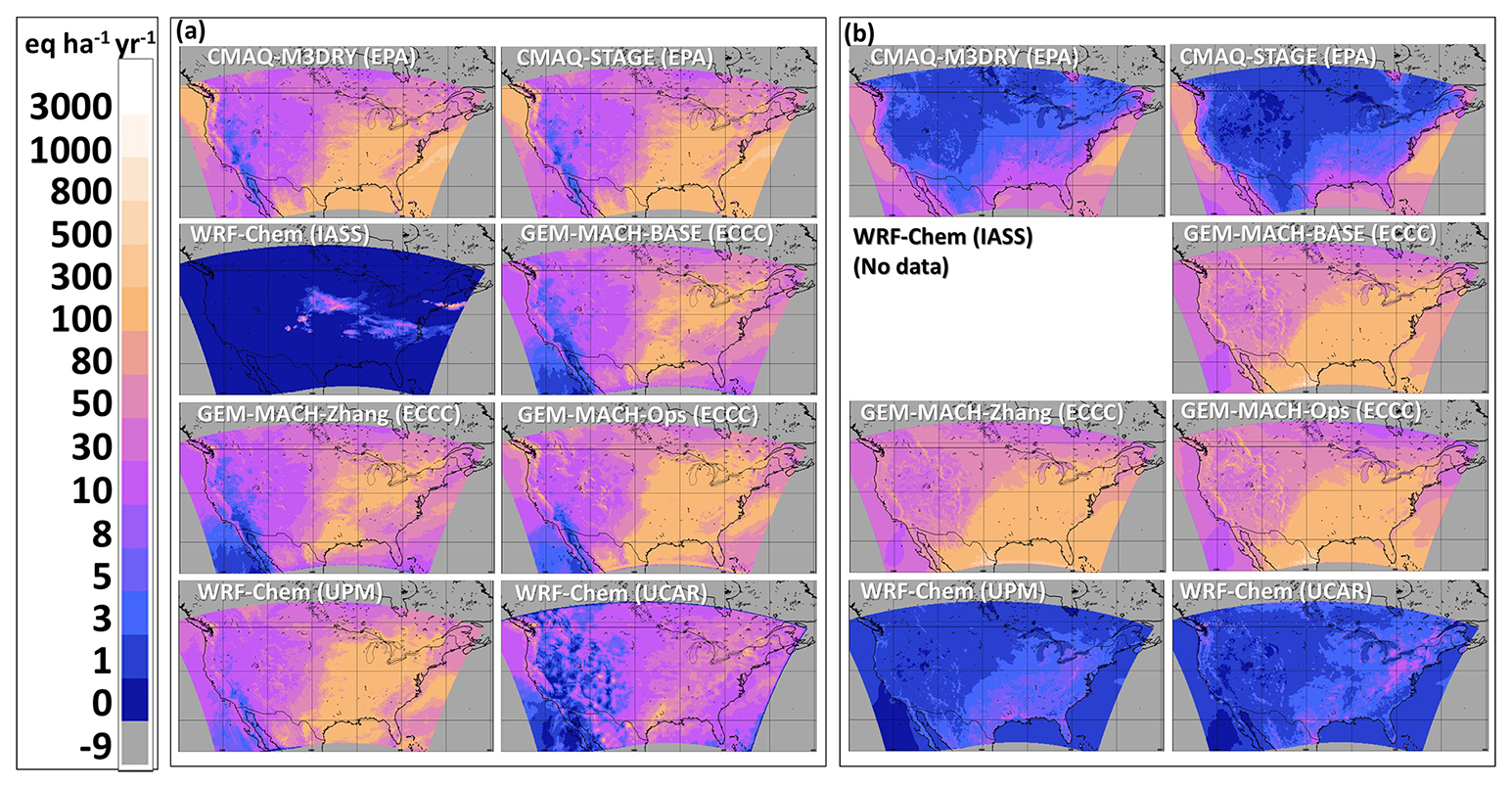
Figure 13 The 2016 total annual deposition flux (eq. ha⁻¹ yr⁻¹) of (a) wet S and (b) dry particulate sulfate. Note that regions outside the AQMEII4 common domain have been assigned an outside-domain mask value of −9.

We next evaluate each of the models' predictions against North American network observations for concentrations of SO₂ and particulate sulfate and sulfur wet deposition for the year 2016. The monitoring network databases employed included the U.S. Environmental Protection Agency Air Quality System (AQS; https://www.epa.gov/aqs, last access: 7 July 2024), the National Atmospheric Deposition Program National Trends Network (NADP NTN; https://nadp.slh.wisc.edu/networks/national-trends-network/, last access: 7 July 2024), the Canadian National Air Pollution Surveillance (NAPS) program (https://www.canada.ca/en/environment-climate-change/services/air-pollution/monitoring-networks-data/national-air-pollution-program.html, last access: 7 July 2024), and the Canadian National Atmospheric Chemistry database (https://www.canada.ca/en/environment-climate-change/services/air-pollution/monitoring-networks-data/national-atmospheric-chemistry-database.html, last access: 7 July 2024).

The NA models' monthly average values of hourly near-surface SO₂(g) concentrations and daily PM_2.5 sulfate concentrations are compared to observations in Fig. 14. The monthly averages of daily (Canadian Air and Precipitation Monitoring Network, CAPMoN) and weekly (NADP) S wet deposition are shown in Fig. 15. Model–observation evaluation statistics are compared in Table S2 (Supplement). Station locations for the observations are shown in Supplement Figs. S15, S16, and S17.

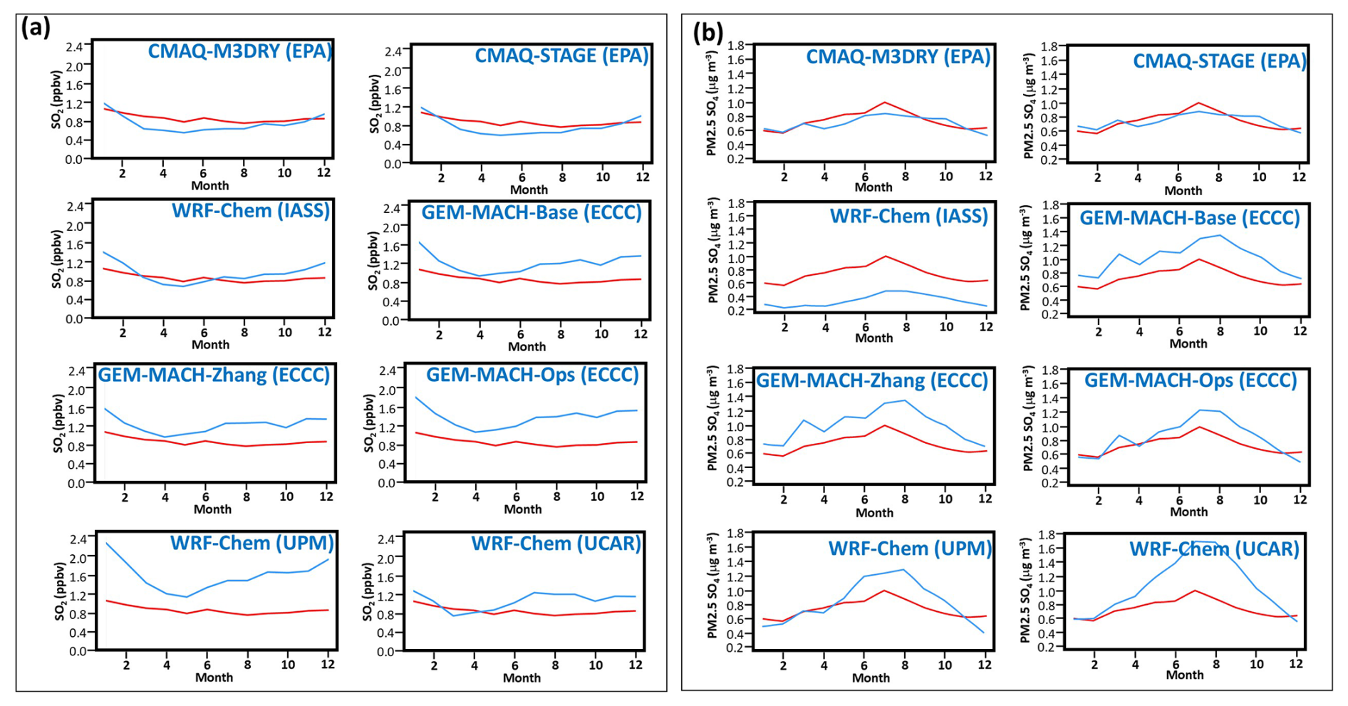
Figure 14 Comparison of model (blue line) and observed (red line) monthly average surface concentrations of (a) hourly SO₂ (ppbv) and (b) daily PM_2.5 sulfate (µg m⁻³) for the year 2016 (AQS, NAPS data).

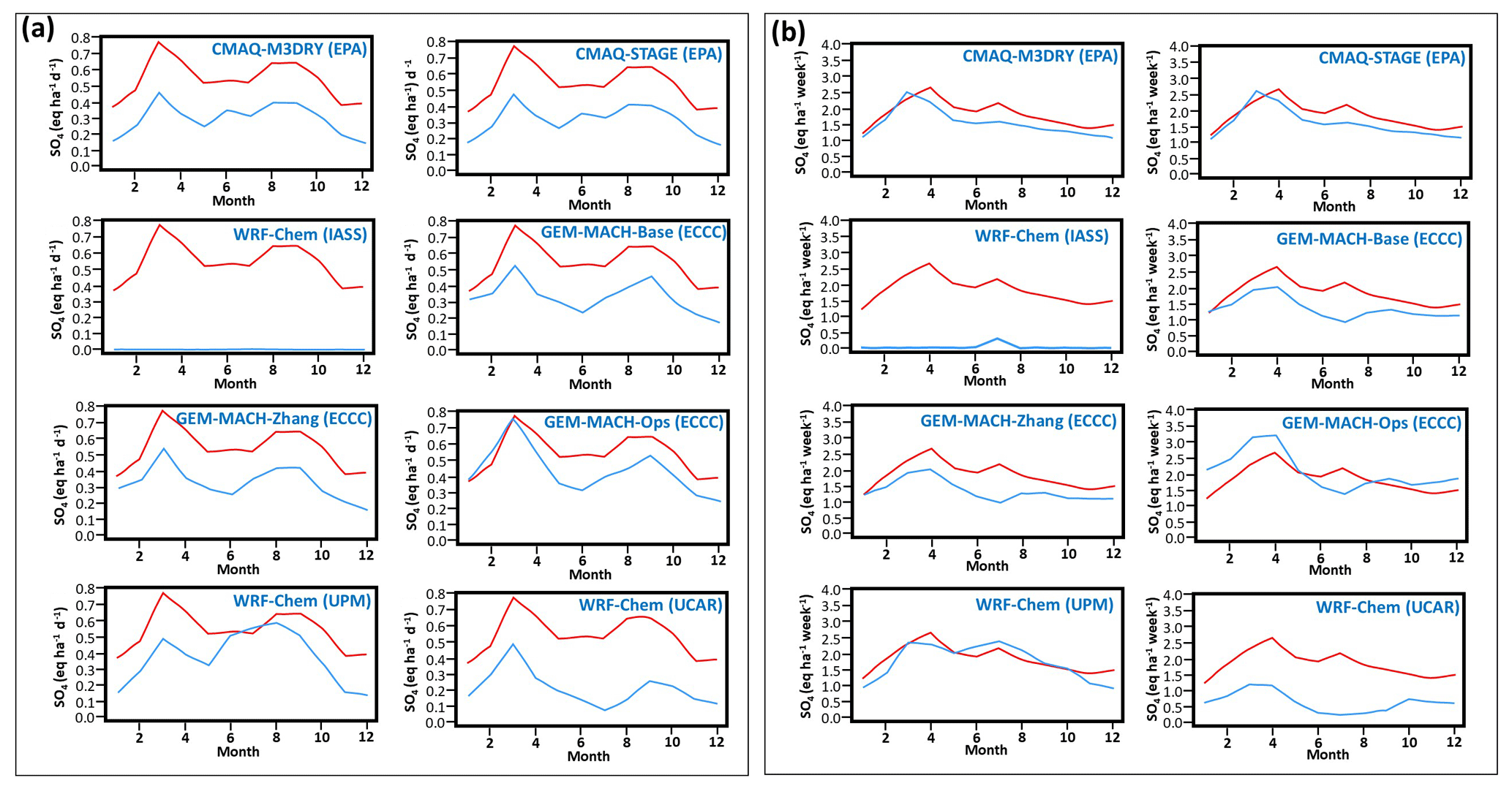
Figure 15 Comparison of model (blue line) and observed (red line) monthly average values of sulfur wet deposition for (a) daily CAPMoN data (eq. ha⁻¹ d⁻¹) and (b) weekly NADP data (eq. ha⁻¹ per week) for the year 2016.

Table S2 shows that CMAQ-M3Dry and CMAQ-STAGE had the best values for most metrics, for the concentrations of SO₂ and PM_2.5 sulfate, and for daily sulfur wet deposition. CMAQ-M3Dry, CMAQ-STAGE, and WRF-Chem (IASS) had predominantly negative biases, and all other models had positive biases. The same tendency can be seen in Fig. 14a, where CMAQ-M3Dry and CMAQ-STAGE negative biases can be seen to occur in the warmer months, whereas WRF-Chem (IASS) has negative biases in the spring. Despite these differences, the net contribution of SO₂ dry-deposition flux to total sulfur deposition on an annual basis is relatively similar across the models (Table 4), with the standard deviation being relatively small, mostly driven by the SO₂ deposition flux for WRF-Chem (UPM) being higher than for the other models.

Particle sulfate (Fig. 14b and Table S2) values were also closest to monthly observed values for CMAQ-M3Dry and CMAQ-STAGE, while they were biased negative for WRF-Chem (IASS) and biased positive for the remaining models. The evaluation of total S wet deposition (Fig. 15a, Table S2) showed that all models with the exception of GEM-MACH (Ops) had negative biases relative to the Canadian daily S wet-deposition observations. Weekly S wet-deposition biases are also negative for most models (Table S2, Fig. 15b), with only GEM-MACH (Ops) having a positive bias in the ensemble.

Factors aside from emissions which affect the SO₂ concentrations within the models are the loss processes of gas oxidation, uptake into hydrometeor water (and subsequent in-cloud oxidation), and dry deposition. Both the gas oxidation and hydrometeor uptake pathways may lead to particulate sulfate formation (through nucleation/condensation of sulfuric acid into particles and through evaporation of hydrometeors). An underestimate of chemical conversion of SO₂ within hydrometeors may thus be expected to result in underestimates of particulate sulfate and in sulfate ion wet deposition. However, Table S2 shows relatively little bias for PM_2.5 sulfate relative to observations for CMAQ-M3Dry and CMAQ-STAGE and positive biases for the GEM-MACH models and WRF-Chem (UPM); these positive biases in predicted particulate sulfate would argue against an insufficient conversion of SO₂ to particulate sulfate in the latter group of models. Rather, the general tendency of negative biases in sulfur wet deposition may indicate insufficient hydrometeor scavenging and subsequent aqueous-phase oxidation of aerosols across all models. We also note that the mean bias of SO₂ concentrations for GEM-MACH (Ops) is more positive than those of GEM-MACH (Base) and GEM-MACH (Zhang), while the particulate sulfate bias was lower and the sulfate wet-deposition bias was higher. GEM-MACH (Ops) makes use of an operational weather forecast for cloud fields, while GEM-MACH (Base) and GEM-MACH (Zhang) make use of an explicit cloud microphysics scheme, which allows for weather–air quality feedbacks to be simulated but tends to underestimate the cloud amounts when used at lower resolution such as the 10 km grid cell size used in the simulations for these three models in this study. The differences between GEM-MACH (Base), GEM-MACH (Zhang), and GEM-MACH (Ops) may thus reflect weaker scavenging of aerosols into clouds in the Base and Zhang implementations.

GEM-MACH (Base), GEM-MACH (Zhang), and WRF-Chem (UCAR) have the most positive biases for particulate sulfate. As noted above, GEM-MACH (Base) and GEM-MACH (Zhang) share a common framework, and unlike other models in the ensemble, they also share an implementation of the updated particle deposition parameters of Emerson et al. (2020). The Emerson et al. (2020) implementation makes use of extensive measurement data and, compared to earlier parameterizations such as Zhang et al. (2001), results in decreased dry-deposition velocities for submicrometre particles and increased dry-deposition velocities for particles larger than 0.2 to 0.8 µm diameter, depending on land use type. The increased PM_2.5 SO₄ values in GEM-MACH (Base) and GEM-MACH (Zhang) in Fig. 14b may thus reflect decreases in the deposition removal flux in the submicrometre portion of the bins in this 12-bin sectional model framework. WRF-Chem (UPM) and WRF-Chem (UCAR) are also both sectional models making use of a common modelling framework, with WRF-Chem (UPM) being a slightly earlier release than WRF-Chem (UCAR). Neither model made use of the Emerson et al. (2020) update at the time the AQMEII4 simulations took place. However, this option was later examined for the WRF-Chem (UCAR) configuration by Ryu and Min (2022), who found that the Emerson et al. (2020) dry-deposition parameterization, applied following the runs carried out here, resulted in an increase in the positive PM_2.5 bias from +4.5 to +6.7 µg m⁻³ and a shift towards less negative biases in PM₁₀ from −19.7 to −1.77 µg m⁻³, similar to the biases in particulate sulfate and ammonium observed in Fig. 14b between GEM-MACH (Base), GEM-MACH (Zhang), and GEM-MACH (Ops). Ryu and Min (2022) further found that the additional update of replacing the default Slinn (1984) aerosol cloud scavenging parameterization with the Wang et al. (2014) parameterization offset the increase in PM_2.5 SO₄ biases associated with the new particle dry-deposition scheme, illustrating the extent to which combinations of parameterizations are sometimes needed to improve model performance. More recent versions of GEM-MACH also make use of multiphase hydrometeor partitioning, with and without the Wang et al. (2014) semi-empirical scavenging scheme, with a significant increase in the uptake of particulate sulfate depending on precipitation rate and improvements in the wet sulfate performance relative to previous model versions (Ghahreman et al., 2024). Implementation of both updated particle dry-deposition velocities and wet-scavenging methodology have thus resulted in reduced biases for these fields, for several of the models examined here, in work following the simulations for AQMEII4.

With regards to sulfur wet deposition, Fig. 15a and Table S2 show a tendency of most models towards negative biases for total daily S wet deposition. However, this negative bias is much less pronounced or even positive in comparison to the weekly S wet-deposition data. Other metrics of model performance differed sharply between the two wet-deposition observation datasets for some metrics, with the weekly wet SO${}_{\mathrm{4}}^{\mathrm{2}-}$ deposition data comparison having higher mean gross error (MGE), normalized mean gross error (NMGE), and root mean square error (RMSE) values than the daily wet SO${}_{\mathrm{4}}^{\mathrm{2}-}$ deposition data comparison. The overall tendency of the performance was similar for both datasets, with the CMAQ models having the best scores for metrics other than mean bias. We note that the daily and weekly NA wet-deposition values correspond to monitoring networks in two different locations (see Fig. S15a). The daily values are from the Canadian CAPMoN network (stations in the AQMEII4 common domain are located mostly in southeastern Canada), while the weekly data from the US NADP network are distributed throughout the USA. The differences in model performance may thus reflect regional differences in predicted meteorological and/or emission fields.

One possible cause for the negative biases in wet deposition common to most models could be underestimates in the amount of model-predicted precipitation, which in turn would reduce the wet flux. The net precipitation totals converted to liquid water for the eight NA models and observations are shown in Fig. S18, for both daily (CAPMoN) and weekly (NADP) monthly averages. While the monthly averages of daily precipitation (Fig. S18b) suggest a tendency towards negative biases in the summer months for some models, the time series of the precipitation biases does not follow that of the sulfate wet-deposition biases; for example, the difference relative to wet sulfate observations in Fig. 15a remains relatively constant for CMAQ-M3Dry and CMAQ-STAGE, while the predicted precipitation difference relative to observations for the same models in Fig. S18a shows more negative biases in the summer than wintertime. Model total precipitation biases thus do not appear to be a major contributing factor to the sulfur flux biases found in this work.

We also note the potential for the lower-magnitude biases in the daily wet SO${}_{\mathrm{4}}^{\mathrm{2}-}$ evaluation, compared to the weekly evaluation, to be the result of the respective regions represented by the two monitoring networks. Figure S16a shows that the daily data are derived from a smaller geographic area than the weekly data; hence regional performance differences may be affecting the two evaluation results.

Summary: North American S deposition variability

Sulfur deposition results from a complex balance between SO₂ oxidation, particulate sulfate formation, scavenging, and the release of particles within clouds, in addition to the processes governing deposition of each of the components. The largest contributing pathways to North American sulfur deposition, in descending order of importance, were wet deposition (SO${}_{\mathrm{4}}^{\mathrm{2}-}$ + HSO${}_{\mathrm{3}}^{-}$), particulate sulfate dry deposition, and dry SO₂(g) deposition in the reduced ensemble of model runs. The largest contributors to model-to-model variability in sulfur deposition, in descending order of importance, were particulate sulfate dry deposition, wet deposition (SO${}_{\mathrm{4}}^{\mathrm{2}-}$ + HSO${}_{\mathrm{3}}^{-}$), and dry SO₂(g) deposition.

CMAQ-M3Dry, CMAQ-STAGE, and GEM-MACH (Ops) had both the highest levels of wet deposition and also the best scores relative to wet-deposition observations. Models with higher PM_2.5 sulfate positive biases relative to observations also had stronger negative biases for sulfate wet deposition, indicating that the magnitude of particle scavenging in hydrometeors may play a role in both biases in the models. Comparisons between GEM-MACH (Base), GEM-MACH (Zhang), and GEM-MACH (Ops) provide some evidence for this effect. WRF-Chem (UPM) and WRF-Chem (UCAR) have very low particulate sulfate deposition fluxes relative to the other models and substantial positive biases in PM_2.5 sulfate and negative biases in sulfate wet deposition, relative to observations, likely related to insufficient wet scavenging of sulfate particles in hydrometeors (Ryu and Min, 2022)

3.2.2 Causes of N deposition variability in North American domain simulations

The common-grid spatial average and percent contribution of each of the species contributing to total annual N deposition for 2016 are given in Table 5. The columns in the table are arranged in descending order from left to right regarding contribution to the reduced-ensemble total nitrogen deposition for each contributing chemical (row labelled “Red. ens. avg”). The impact of variability on the model deposition from each component for each model is once again shown as the standard deviation across the models used for the reduced ensemble (row labelled “Red. ens. SD”). From the row representing the standard deviation, it can be seen that the variation (standard deviation) between models for the contributions to total N deposition are driven, in descending order, by particle ammonium (DAM column, where the standard deviation for particle ammonium deposition is larger than the reduced-ensemble mean value), followed by wet ammonium ion (WNH4), wet nitrate ion (WNO3), dry HNO₃ (DHNO3), dry particle nitrate (DNI), dry NO₂ (DNO2), and dry ammonia gas (DNH3), with the remaining species contributing a small percentage of the total variability. Both the particle ammonium and wet ammonium variability between the models is largely driven by the GEM-MACH group of models, which have average dry particle ammonium and wet ammonium fluxes which are 17.4 and 1.76 times higher than the other models, respectively.

We next evaluate the models' nitrogen performance using the available concentration and wet-deposition flux data to determine the impact of the parameterization differences on model performance and hence identify which components in which models might be improved.

Table 5 Contributions of N species to total deposition (eq. ha⁻¹ yr⁻¹) and percent of total N deposited, over the NA AQMEII4 common grid, arranged in descending order of importance to the reduced-ensemble average. WNH4: wet deposition of NH${}_{\mathrm{4}}^{+}$(aq). DHNO3: dry deposition of HNO₃(g). WNO3: wet deposition of NO${}_{\mathrm{3}}^{-}$(aq). DAM: dry deposition of particulate ammonium. DNH3: dry deposition of NH₃(g). DNI: dry deposition of particulate nitrate. DNO2: dry deposition of NO₂(g). DPAN: dry deposition of peroxyacetyl nitrate gas. DRN3: dry deposition of gaseous organic nitrate gases. DN2O5: dry deposition of N₂O₅(g). DHNO4: dry deposition of pernitric acid gas. DNO: dry deposition of NO(g). WRF-Chem (IASS) did not report dry particle fluxes. The GEM-MACH models and WRF-CHEM (UPM) do not include dry deposition of N₂O₅(g), and the GEM-MACH models do not dry deposit HNO₄(g). n/d: no data.

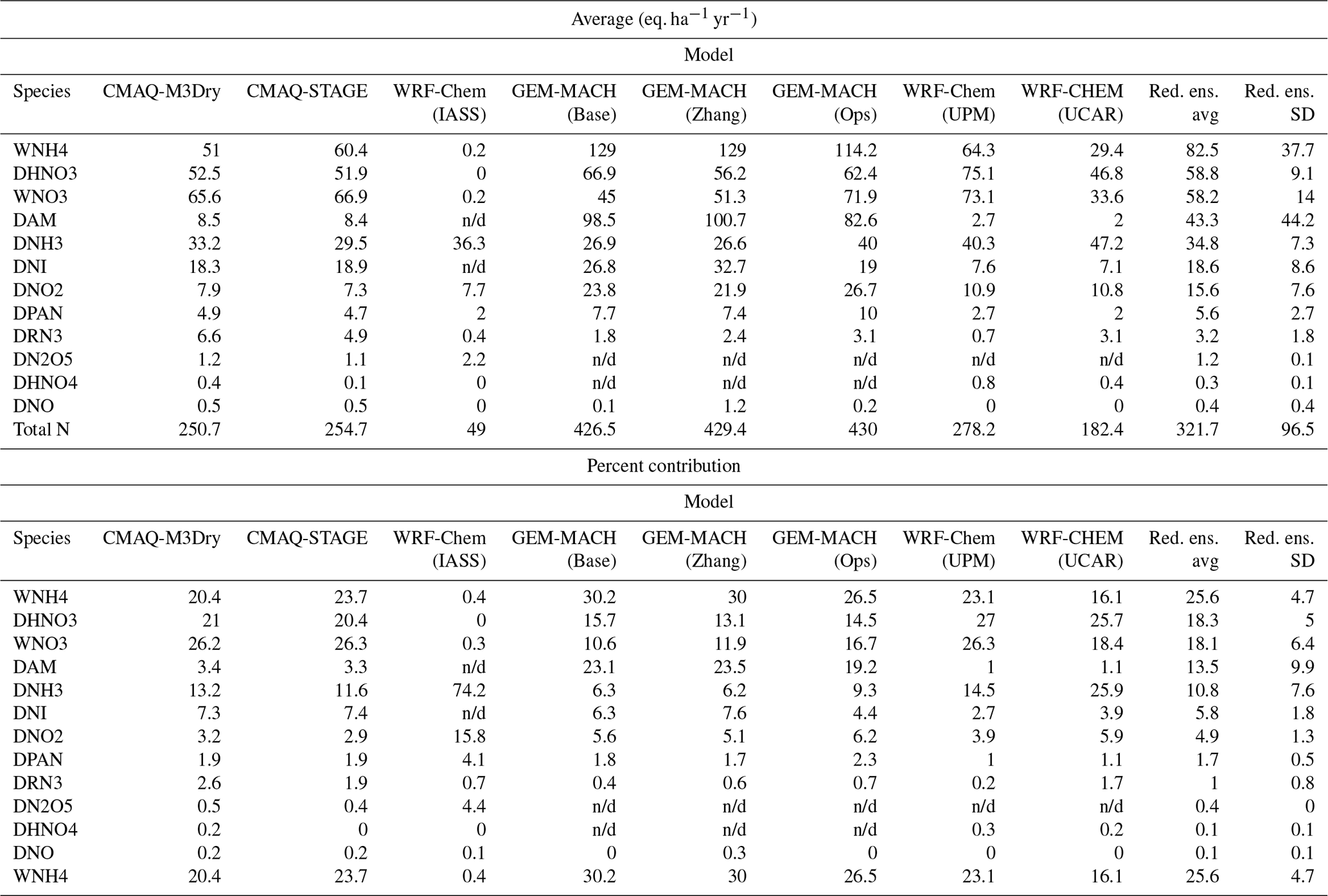
Dry deposition of particle ammonium

The largest source of variability between North American models' total N predictions resides in the dry particle ammonium deposition fluxes, with Table 5 showing that the standard deviation of this deposition flux across models was essentially as large as the reduced-ensemble average. Particle ammonium dry deposition contributes a disproportionately high contribution to total N variability across the North American ensemble, despite the magnitude of the ensemble average particle ammonium dry-deposition flux being less than the deposition of wet ammonium ion, dry nitric acid gas, or wet nitrate ion.

Figure 16 compares the monthly average PM_2.5 ammonium concentrations with observations (station locations appear in Fig. S15b), and Table S3 provides detailed statistics. From the latter, CMAQ-M3Dry and CMAQ-STAGE have the best overall performance for particulate ammonium and GEM-MACH (Base), GEM-MACH (Zhang) and GEM-MACH (Ops) have the worst performance by the statistical measures used here. This latter group of models also have the largest magnitude of positive biases relative to observed PM_2.5 ammonium concentrations, while the CMAQ implementations have negative biases and the remaining models have smaller-magnitude positive biases. Figure 16 shows that CMAQ-M3Dry, CMAQ-STAGE, WRF-Chem (IASS), and to a lesser extent WRF-Chem (UPM) have a greater seasonal variability in model particle ammonium (blue line) than observed (red line), with the difference between summer and winter (months 1 and 12 versus months 5 through 9) being higher in the models than in observations.

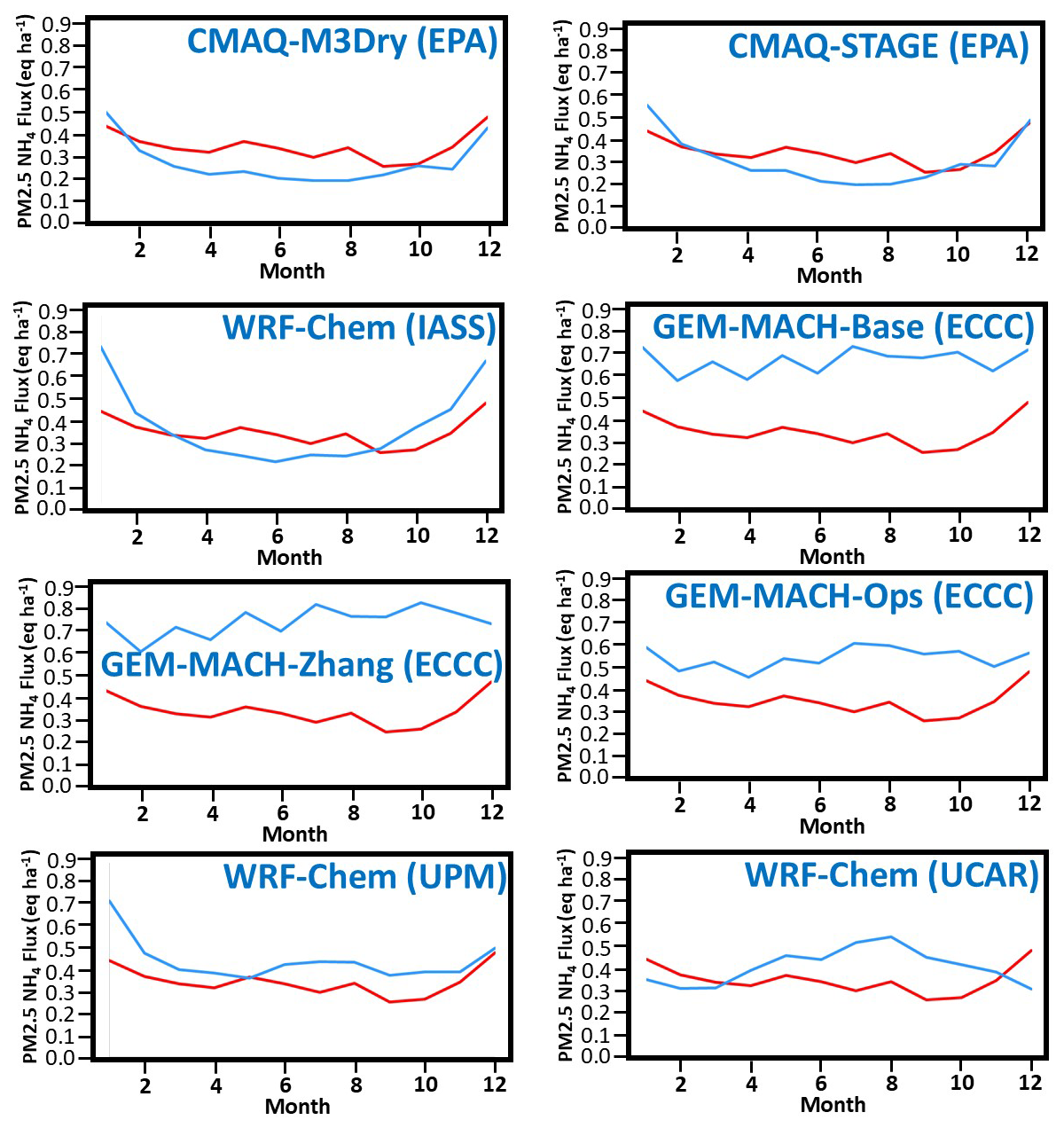
Figure 16 PM_2.5 ammonium compared to observations, North American model ensemble for the simulation year 2016. Red line: monthly observed average. Blue line: monthly model average.

The GEM-MACH contributions to model N variability in critical load exceedances are thus linked to poor model performance for PM_2.5 ammonium. This poor performance is likely due to two factors, which can be deduced from comparing the process representations implemented in the models (Sect. 2.2).

The first factor, which differentiates GEM-MACH (Base), GEM-MACH (Zhang), and GEM-MACH (Ops) from the other ensemble members relates to how inorganic aerosol thermodynamic partitioning chemistry has been implemented: while the process representation in the models of the ensemble is derived from the ISORROPIA module (Nenes et al., 1998; Fountoukis and Nenes, 2007), the GEM-MACH implementations in AQMEII4 employ a partial speciation of SO${}_{\mathrm{4}}^{\mathrm{2}-}$, NH${}_{\mathrm{4}}^{+}$, and NO${}_{\mathrm{3}}^{-}$ (Makar et al., 2003) and do not include the reactions involving particulate base cations (Ca²⁺, Mg²⁺, Na⁺, K⁺). The other models in the ensemble do include these additional reactions. In the absence of base cation chemistry, the formation of particle ammonium will be controlled by the availability of ammonia gas in excess of that required to charge balance particulate sulfate, as well as by the availability of nitric acid gas. In the presence of base cations, nitric acid gas will preferentially associate with base cations rather than ammonia, leaving less HNO₃ available for particle ammonium nitrate formation. Several observational studies have shown that when base cations are present, their peak mass occurs in the coarse particle size mode (>2.5 µm diameter), where they will have higher deposition velocities (e.g. inland, agricultural dust sources (Makar et al., 1998); ocean sources of sea-salt (Anlauf et al., 2006)). Base cation inorganic heterogeneous chemistry thus provides a competing pathway for the uptake of nitrate into particles and, when present, will also reduce the amount of NH₃ that may be taken up by particles, especially in the fine mode. The positive bias of PM_2.5 ammonium in Fig. 16 for GEM-MACH relative to the other models likely represents the impact of simplified inorganic aerosol chemistry.

The second factor influencing the GEM-MACH models' positive particulate ammonium biases may be reflected in the biases for GEM-MACH (Base) and GEM-MACH (Zhang), which are higher by 50 % to a factor of 2 than that of GEM-MACH (Ops), respectively; that is, an additional source of bias resides in the former two model implementations that is not present in the latter implementation. The likely source of this additional bias is the use of Emerson et al. (2020) particle deposition velocities in these implementations, in the absence of enhanced wet scavenging of aerosols, as discussed above for PM_2.5 sulfate and described in Ryu and Min (2022) and Ghahreman et al. (2024). Ryu and Min (2022) showed that the use of the updated particle deposition velocity as per Emerson et al. (2020), when implemented in the absence of concurrent multiphase wet-scavenging updates, led to positive biases in PM^2.5 concentrations in the WRF-Chem model.

We note that the manner in which inorganic heterogeneous chemistry is simulated also differs between the models. CMAQ-M3Dry and CMAQ-STAGE calculate local equilibrium concentrations at different modes of the size distribution, and WRF-Chem (UPM) and WRF-Chem (UCAR) also calculate the equilibrium with respect to specific size bins, while GEM-MACH (Base), GEM-MACH (Zhang), and GEM-MACH (Ops) carry out a single bulk calculation across all size bins. The use of a bulk calculation is a third simplification for the latter group of models and may also affect the particulate ammonium performance of these models.

The spatial distribution of PM_2.5 ammonia biases was examined in Fig. 17, for the month of July 2016 (July was chosen due to the expectation that bidirectional fluxes would have a higher impact in the summer months). The region with the highest positive biases (dark-red circles, Fig. 17) are in the same station locations for all models, in the agricultural region to south of the Great Lakes. Positive PM_2.5 ammonium mean biases also occur near urban regions in the western USA (Seattle–Tacoma, Yakima, Portland, Sacramento, San Jose, Boise, Butte, Helena, Denver, Boulder, and Albuquerque) and at one eastern site, Miami. A re-examination of ammonia gas deposition and emission parameters and primary particle ammonium emission inventories is recommended for these locations, given that they are likely having a large impact on model performance statistics. The CMAQ models and WRF-Chem (IASS) have negative to minimal biases along the coastlines and southwestern USA (regions of sea-spray NaCl and windblown base cation containing dust, respectively), while WRF-Chem (UPM) and WRF-Chem (UCAR) have small negative to positive biases in these regions and the GEM-MACH models are uniformly biased positive in these regions. This provides support for the possibility that the GEM-MACH positive bias in particulate ammonium concentrations is due to missing particulate base cation chemistry; the regions where particulate base cations would be expected to contribute significantly to total particulate mass are also the regions where the GEM-MACH models have positive biases, and the biases in the other model biases are not as significant.

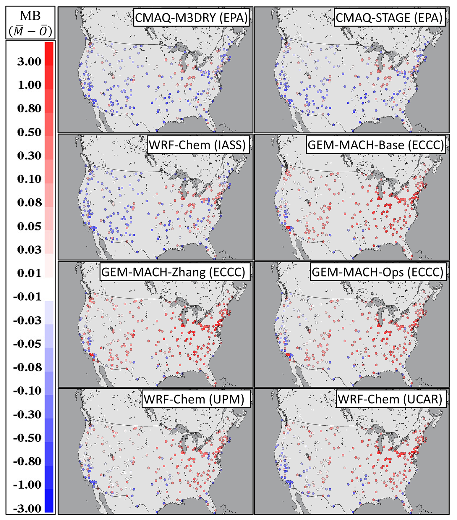
Figure 17 Mean bias (MB = $\stackrel{\mathrm{‾}}{M}-\stackrel{\mathrm{‾}}{O}$, where $\stackrel{\mathrm{‾}}{M}$ is the model mean and $\stackrel{\mathrm{‾}}{O}$ is the observed mean), PM_2.5 NH₄, July 2016, by station (µg m⁻³). Negative values are given in blue; positive biases are given in red. Note that the colour scale is logarithmic.

Wet deposition of ammonium and nitrate ions

Wet deposition of ammonium ion is the largest contributor to the North America reduced-ensemble N_dep and the second largest contributor to model-to-model variability in N deposition (Table 5). Wet deposition of nitrate ion is the third largest contributor to both the NA ensemble total N deposition and model-to-model variability in N deposition. Time series of the monthly averages of observed and modelled daily (CAPMoN) and weekly (NADP) NH${}_{\mathrm{4}}^{+}$ wet-deposition fluxes are shown in Fig. 18. The monthly mean of modelled daily values (Fig. 18a) are generally biased negative, with the exceptions of the months of July and August for GEM-MACH (Base) and GEM-MACH (Zhang). The observed maximum in NH${}_{\mathrm{4}}^{+}$ wet deposition occurs in April (Fig. 18a, red line, month 4); this seasonal variation is captured only by GEM-MACH (Ops) and WRF-Chem (UCAR), with the other models predicting peak deposition in June through August. The monthly average of the weekly NH${}_{\mathrm{4}}^{+}$ wet-deposition fluxes (Fig. 18b) shows a similar pattern, with the observed values (red lines, Fig. 18b) peaking in April and all of the models except for WRF-Chem (UCAR) peaking in June. As was the case for sulfate wet deposition, the observed seasonal variation is apparently not connected with biases in precipitation predictions (see Fig. S18a and b and the Supplement), with the possible exception of WRF-Chem (UCAR), for which total precipitation is biased substantially negative throughout the year.

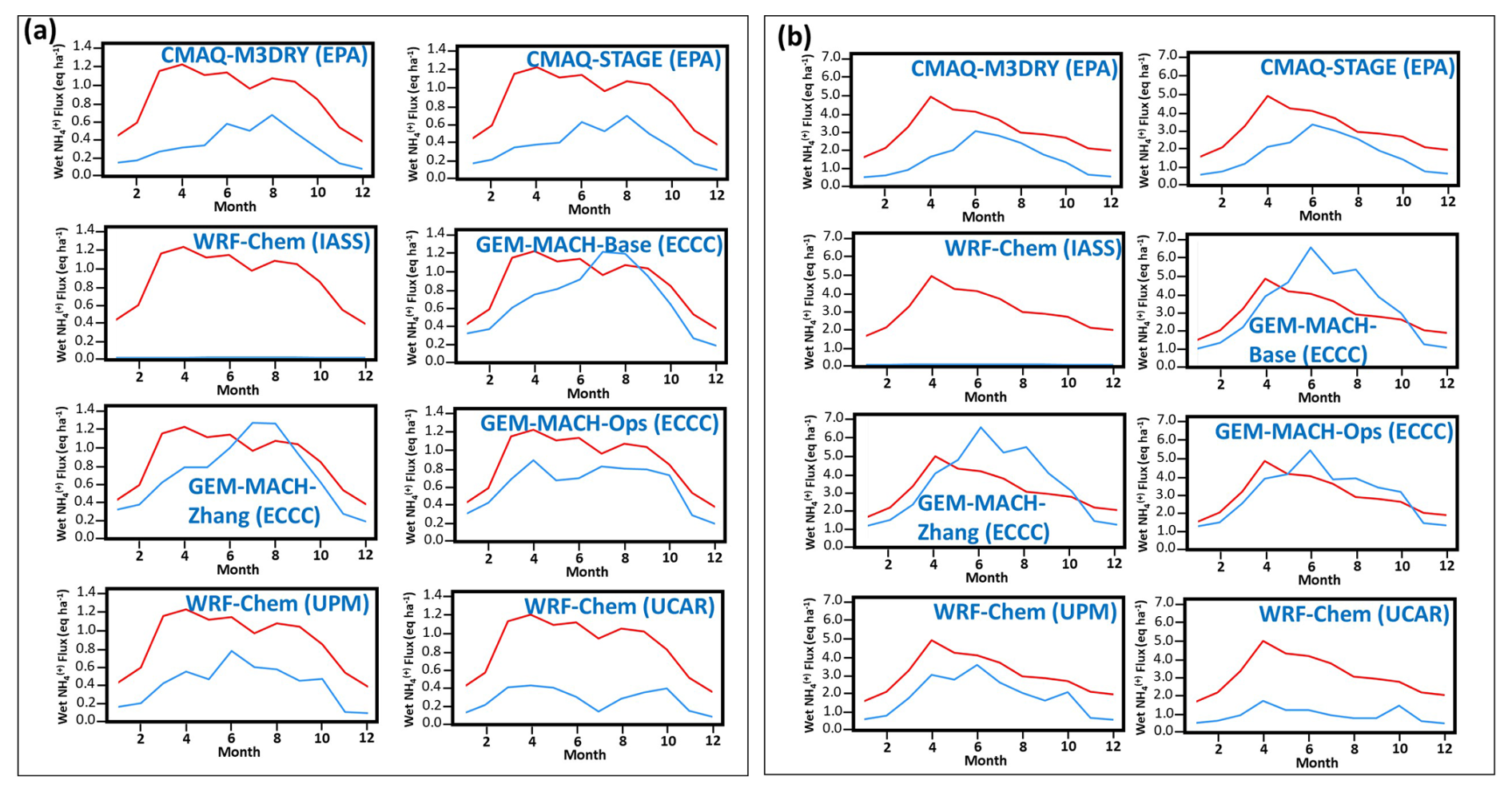
Figure 18 Time series of monthly average observed (red line) and modelled (blue line) ammonium wet-deposition fluxes for (a) daily CAPMoN data (eq. ha⁻¹ d⁻¹) and (b) weekly NADP data (eq. ha⁻¹ per week).

As noted above, the models taking part in this ensemble did not make use of multiphase hydrometeor scavenging in precipitation. The maximum NH${}_{\mathrm{4}}^{+}$ wet-deposition negative bias in April featuring for several models may reflect the absence of this level of detail in hydrometeor scavenging, with the absence of snow scavenging potentially impacting early-spring deposition. We note that the weekly and daily monitoring networks cover different geographical regions, hence the differences in model performance relative to the two observation datasets (compare the CAPMoN and NADP station locations in yellow and green circles in Fig. S15a, respectively).

The mean biases in average daily and weekly NH${}_{\mathrm{4}}^{+}$ wet deposition for the month of April are shown in Fig. 19. WRF-Chem (IASS), CMAQ-M3Dry, and CMAQ-STAGE have predominantly negative biases throughout the region; WRF-Chem (UCAR) and WRF-Chem (UPM) have a few stations with more positive biases; and the GEM-MACH models have both positive and negative biases throughout the domain. Insight into the differences in model performance can be gained through reviewing the manner in which each model parameterizes aerosol activation and scavenging:

1. GEM-MACH (Base), GEM-MACH (Zhang), GEM-MACH (Ops), WRF-Chem (UPM), and WRF-Chem (UCAR) make use of the aerosol activation scheme of Abdul-Razzak and Ghan (2000) and the Slinn (1984) approach to aerosol scavenging.

2. In GEM-MACH (Ops), the aerosol activation and aerosol-scavenging schemes are decoupled from meteorological feedbacks, while GEM-MACH (Base), GEM-MACH (Zhang), WRF-Chem (UPM), and WRF-Chem (UCAR) are “aerosol-aware” and full feedback models incorporating parameterizations for the aerosol direct and indirect effects. The latter will result in cloud formation from model-produced aerosols acting as cloud-condensation nuclei; clouds are more likely to form where aerosol concentrations are high (and thus more likely to scavenge aerosols below the clouds as well), compared to offline models. Very high aerosol concentrations may also reduce cloud droplet size and cloud-to-precipitation conversion, potentially making clouds more persistent, while reducing precipitation.

3. WRF-Chem (IASS) also makes use of aerosol direct- and indirect-effect feedbacks but employs the approach of Chapman et al. (2009) for aerosol scavenging.

4. CMAQ-M3Dry and CMAQ-STAGE are offline models (no feedbacks between aerosols, cloud formation, and radiative transfer takes place), where interstitial and nucleation aerosol scavenging by cloud droplets is modelled following Binkowski and Roselle (2003), and the wet-deposition rate is a simple parameterization dependent on the cloud total liquid water content, cloud thickness, and cloud precipitation rate (Fahey et al., 2017).

The Slinn (1984) aerosol-scavenging approach makes use of different observation-based aerosol collection efficiency formulae for rain and snow, respectively, where temperature dependence in the collection efficiency such as at 0 °C may be used to distinguish between liquid and solid hydrometeor collection efficiencies. Following the AQMEII4 simulations carried out here, parameterizations that utilize multiphase precipitation data with multiple hydrometeor classes, such as those of Wang et al. (2014), have been tested within the modelling framework of GEM-MACH (Ghahreman et al., 2024). Similarly, Ryu and Min (2022) describe the impact of multiphase hydrometeor scavenging as implemented in the WRF-Chem modelling framework. These tests resulted in significant improvements in particulate concentrations and wet deposition compared to previous implementations employing the approach of Slinn (1984). The approach for scavenging in Binkowski and Roselle (2003) assumes scavenging only occurs in cloud droplets; snow scavenging is not considered. However, snow scavenging at higher precipitation rates is known to be 1 to 2 orders of magnitude more efficient than scavenging by rain. Hence the use of the Slinn (1984) parameterization instead of multiphase hydrometeor scavenging and the Wang et al. (2014) parameterization in GEM-MACH, as well as the omission of multiphase hydrometeor scavenging in CMAQ, may account for the springtime bias in all models noted here.

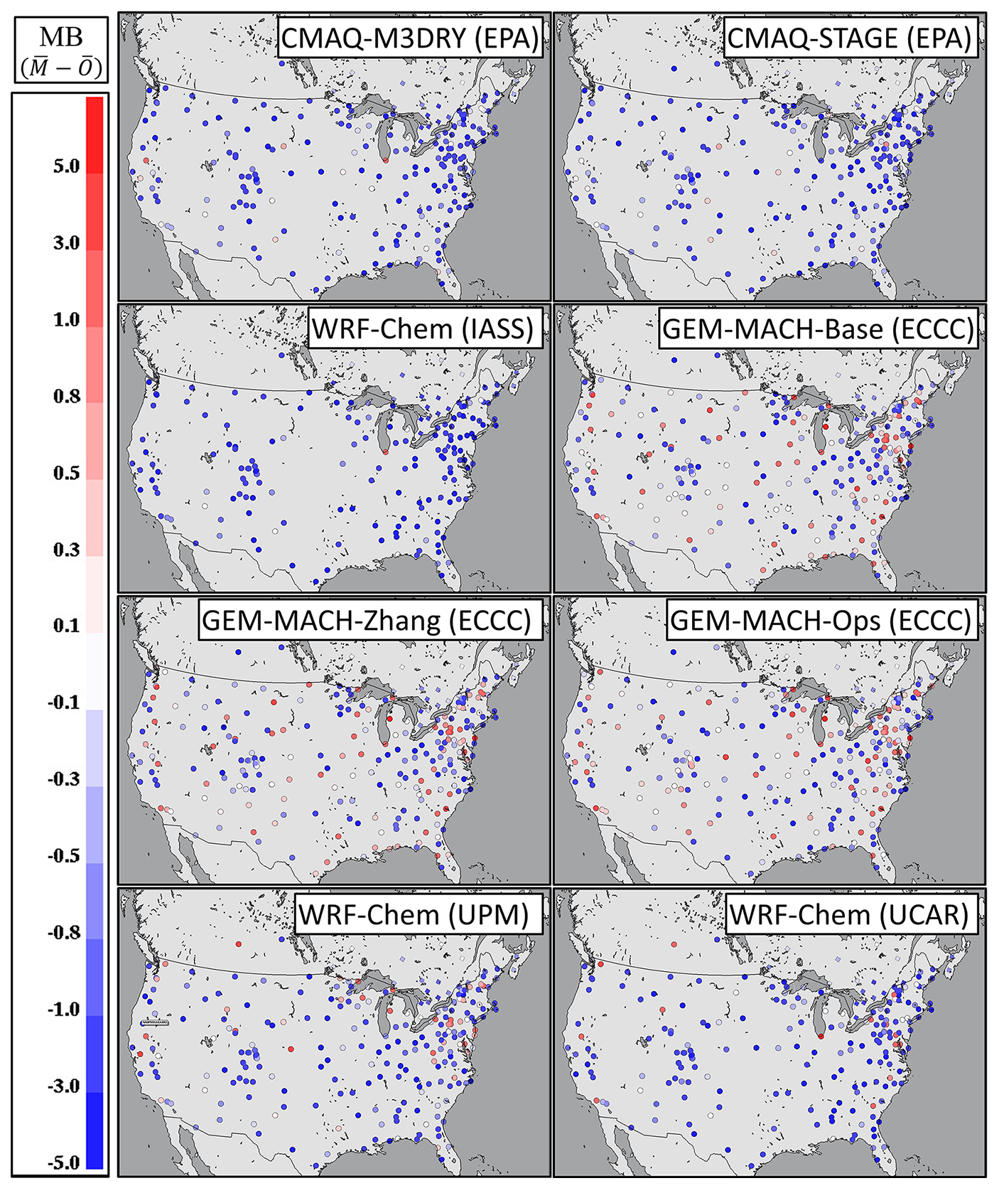
Figure 19 Model mean biases in ammonium wet deposition for the month of April 2016, North America (eq. ha⁻¹ yr⁻¹). Daily station values of the mean bias (CAPMoN network) are shown as diamonds; weekly station values (NADP network) are shown as circles. Positive biases are shown in red; negative biases are shown in blue. Note that the colour scale intervals are logarithmic.

The causes of the differences in wet deposition of NH₄ between WRF-Chem (IASS), WRF-Chem (UPM), and WRF-Chem (UCAR) may be the use of the Chapman et al. (2009) wet-scavenging approach in the first model and the implementation of the Abdul-Razzak and Ghan (2000) and the Slinn (1984) approaches in the latter two models. All three models make use of the Morrison two-moment cloud microphysics scheme (Morrison et al., 2009), though WRF-Chem (IASS) and WRF-Chem (UPM) differ from WRF-Chem (UCAR) in the parameterization of convective clouds (See Table 1). Differences in aerosol-scavenging implementations may account for some of the differences in ammonium wet deposition between these models, as may the manner in which convective clouds identify cloud condensation nuclei from aerosol size distribution and speciation within their convective parameterizations.

Wet nitrate ion deposition is the third largest source of N deposition in the North American ensemble as well as the third largest source of model-to-model variability (Table 5). CMAQ-M3Dry, CMAQ-STAGE, and GEM-MACH (Ops) have the best performance scores for nitrate wet deposition (Table S3 in the Supplement). GEM-MACH (Base) and GEM-MACH (Zhang) have larger-magnitude and more negative biases than GEM-MACH (Ops), despite all three models making use of the same modelling framework. The only difference between GEM-MACH (Base) and GEM-MACH (Zhang) is the gas-phase dry-deposition algorithm employed (see Table 2). The increase in the wet-deposition negative bias magnitude going from GEM-MACH (Zhang) to GEM-MACH (Base) in Table S3 (from −0.19 to −0.26 eq. ha⁻¹ d⁻¹ for daily CAPMoN data and from −0.41 to −0.64 eq. ha⁻¹ d⁻¹ for weekly NADP data) is therefore attributable to gas-phase deposition differences. This is also reflected in the HNO₃ dry-deposition flux for the two models in Table 5, with the deposition flux for GEM-MACH (Base) at 66.9 eq. ha⁻¹ yr⁻¹ being 19 % higher than the GEM-MACH (Zhang) value of 56.2 eq. ha⁻¹ yr⁻¹.

The remainder of the difference in nitrate wet-deposition bias between GEM-MACH (Base) and GEM-MACH (Zhang) and GEM-MACH (Ops) must be due to other factors in the model configuration as described in Table 2. Based on the PM_2.5 sulfate and PM_2.5 nitrate evaluations (Tables S2, S3), as well as the work of Ghahreman et al. (2024) and Ryu and Min (2022), we believe that the cause of the additional wet nitrate negative bias resides in the use of the new particle deposition velocity algorithm in the absence of a simultaneous update in the wet-deposition algorithm to make use of multiphase hydrometeor scavenging of aerosols. For example, the particulate matter scavenging coefficients for snow are 1 to 2 orders of magnitude more efficient than for rain – including snow scavenging (which may occur at higher elevations even in the summer) will lead to greater uptake of particles (Ghahreman et al., 2024). The Emerson et al. (2020) parameterization will lead to less particle deposition in submicrometre particle sizes (and hence would otherwise increase PM_2.5 concentrations – the increased scavenging associated with multiphase hydrometeors will offset this effect).

Dry deposition of HNO₃

Dry deposition of HNO₃ is the second largest source of N_dep in the reduced ensemble and the fourth largest source of model-to-model variability.

The spatial variation in the annual sum of the effective deposition fluxes for HNO₃ dry deposition are shown in Figs. S19, S20, S21, and S22, representing the mass of HNO₃ transferred to the surface via the cuticle, soil, stomatal, and lower-canopy pathways, respectively, and are summarized as common-grid totals in Fig. 20. Effective fluxes build on the concept of effective conductance: the product of the hourly deposition flux with the ratio of specific pathway conductance to total deposition velocity, for each of the four pathways (Galmarini et al., 2021). The figures thus depict the contributions of each pathway to the HNO₃ dry-deposition mass flux for each model¹. Effective fluxes incorporate changes in the flux resulting from changes in chemical concentration associated with factors in addition to deposition. However, comparison of the effective-flux values of Fig. 20 to effective conductances (not shown) has a similar pattern, implying that the deposition velocity is the dominating factor in the HNO₃ deposition flux. The HNO₃ mass flux is dominated by the cuticle pathway (Figs. S19, 20), followed by the soil pathway (Figs. S20, 20). All models show a similar pattern in HNO₃ annual cuticle flux (largest fluxes in the southeastern USA, lowest fluxes over the western mountain ranges and the Canadian boreal forest), though the magnitudes of the fluxes vary, with WRF-Chem (UPM) having the highest flux and GEM-MACH (Zhang) showing much lower fluxes for specific land use types over the western mountains compared to the other models.

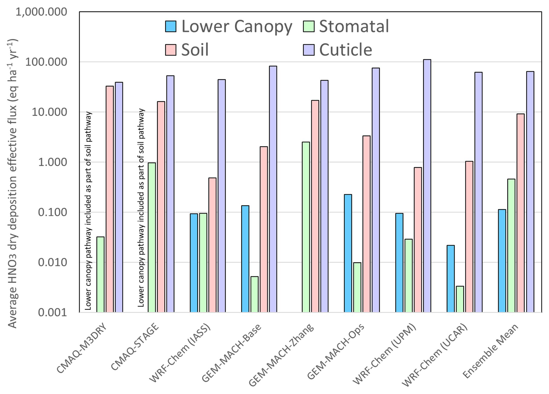
Figure 20 Averages of flux pathway contributions to HNO₃ dry deposition, NA AQMEII4 common grid, 2016 (eq. ha⁻¹ yr⁻¹).

The HNO₃ dry-deposition velocity parameterizations in the GEM-MACH models depend in part on deposition pathway parameterizations employing functions of the ozone and sulfur dioxide pathway values (Makar et al., 2018; Zhang et al., 2003). Other recent AQMEII4 work for ozone dry deposition using an observation-driven single-point modelling framework (Clifton et al., 2023) found that the ozone deposition velocity for GEM-MACH (Base) has positive biases in the summer months (average across eight sites of +73 %) and negative biases in the winter months (eight-site average of −33 %), while GEM-MACH (Zhang) has smaller summer biases (+3 %) and high winter biases (+50 %). This is consistent with the increase in HNO₃ dry-deposition flux going from GEM-MACH (Zhang) to GEM-MACH (Base), though HNO also deposits via dissociation (sulfur dioxide pathway); not all of the observed effects can be attributed to the use of O₃ as a proxy in part of the deposition algorithm. A portion of the increase in the negative bias in nitrate wet deposition going from GEM-MACH (Zhang) to GEM-MACH (Base) is thus the result of the higher HNO₃ dry-deposition removal of the available nitrate which would otherwise be taken up into clouds.

NH₃ and the role of bidirectional flux algorithms

NH₃ deposition fluxes were the fifth largest driver of ensemble nitrogen deposition and the seventh largest driver of N_dep variability in North America. Two different observation datasets for the year 2016 were used to evaluate model NH₃ concentration performance and cross-track infrared sounding (CrIS) satellite retrievals of NH₃ (see the Supplement for retrieval procedure and references) and AMoN (Chen et al., 2014; NADP, 2025b) surface monitoring network observations (see Supplement Fig. S16b for AMoN measurement locations). The two datasets evaluate model NH₃ performance in different ways. The CrIS observations (and model values extracted for evaluation) correspond to the specific time of day of the satellite overpass, for the polar-orbiting platform upon which the CrIS instrument is based. The evaluation against CrIS data is thus a measure of the model performance at early afternoon local time. The AMoN observations in contrast are 2-week integrated average concentrations; the AMoN comparison evaluates average model performance on this integrated timescale and hence includes into that average diurnal variations in NH₃ concentrations not available in the CrIS observations.

The evaluation of the models' NH₃ against CrIS observations at overpass time is shown in Table S4 (Supplement) and Fig. 21. The general trend for the models is one of negative biases in NH₃ concentrations. CMAQ-M3Dry and CMAQ-STAGE have the largest negative NH₃ biases, lowest number of model values within a factor of 2 of the observations (FAC2), highest MGE, lowest R, lowest coefficient of efficiency (COE), and lowest index of agreement (IOA) scores in Table S4. This suggests that the magnitude of the fluxes and/or the balance between positive (downward; deposition) and negative (upward; emission) fluxes for CMAQ-M3Dry and CMAQ-STAGE are the cause of the models' relatively poor performance for NH₃. GEM-MACH (Base) and GEM-MACH (Zhang) have the smallest (and positive) biases compared to the other models, and these two models as well as WRF-Chem (UPM) and WRF-Chem (UCAR) have the best overall scores for NH₃ against satellite data.

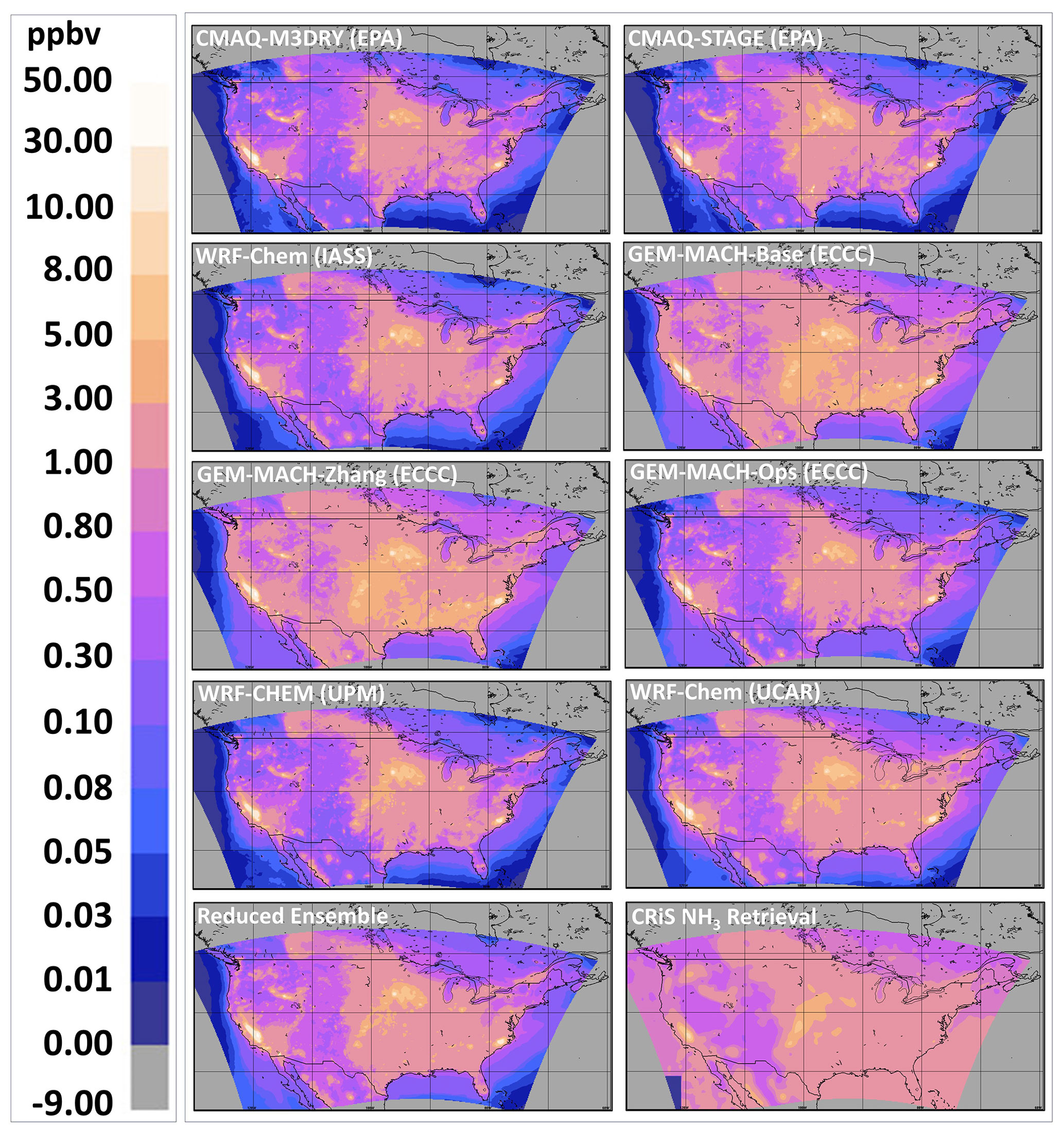
Figure 21 Comparison of annual average surface NH₃ concentrations at CrIS overpass times (participating models and the reduced ensemble) and the corresponding CrIS observed average NH₃ at overpass times. Note that regions outside the AQMEII4 common domain have been assigned an outside-domain mask value of −9.

The satellite data comparison of Fig. 21 also shows some significant differences between observed ammonia and all models' predicted ammonia, particularly over waterbodies (oceans, Great Lakes), with observed NH₃ in the range 1–3 ppbv in the Atlantic and near Baja California, while the models all show NH₃ over the oceans always below 0.3 to 0.5 ppbv and decreasing with increasing distance from the shoreline. All models reach 0.0–0.01 ppbv at the greatest distances from the shoreline, while the satellite observations are above 0.5 ppbv (lower detection limit of ∼ 0.3 ppbv) throughout the AQMEII4 common domain.

NH₃ emissions from natural sources have been a source of ongoing interest in the global modelling community due to its properties as a greenhouse gas. Paulot et al. (2015) reviewed estimates of global oceanic NH₃ emissions, with a range of 7–23 Tg N yr⁻¹ and their own estimate being lower at 2.5 Tg N yr⁻¹. Their estimated maps of NH₃ emissions showed relatively lower values on the western shoreline of North America (Pacific coast) than on eastern shoreline (Atlantic coast) and high emissions in three out of the four oceanic NH₃ flux models tested, in the Gulf of Mexico and along the Gulf Stream between North America and Europe (their Fig. 3). Subsequent simulations of oceanic outgassing (Paulot et al., 2020) showed oceanic outgassing in the Gulf of Mexico in excess of 0.03 g N m⁻² yr⁻¹ (17.6 eq. ha⁻¹ yr⁻¹) and between 0.01 and 0.02 g N m⁻² yr⁻¹ (5.9 to 11.8 eq. ha⁻¹ yr⁻¹) in the Gulf Stream. The oceanic emission model of Paulot et al. (2020) would be relatively straightforward to implement in a regional modelling context; our work suggests that a considerable deficit in oceanic NH₃ may be occurring in the current regional air quality models.

The evaluation of the models' NH₃ against biweekly surface observations at the AMoN sites is shown in Table S5 (Supplement), where biweekly values have been used to create annual averages from both model and observed values at observation sites. GEM-MACH (Base) and GEM-MACH (Zhang) once again have the lowest-magnitude (and positive) biases relative to observations; CMAQ-M3Dry and CMAQ-STAGE have the most negative biases, though CMAQ-STAGE has the best correlation coefficient score; and WRF-Chem (UPM) has the best scores overall aside from the mean bias and correlation coefficient.

Figure 22 shows the contributions to total N deposition flux from the dry deposition of NH₃(g) and the difference in overall deposition patterns between the models employing bidirectional NH₃ flux parameterizations (CMAQ-M3Dry, CMAQ-STAGE, GEM-MACH (Base), and GEM-MACH (Zhang)) and the models which do not employ such a parameterization (WRF-Chem (IASS), GEM-MACH (Ops), WRF-Chem (UPM), WRF-Chem (UCAR)). The models utilizing bidirectional fluxes have large regions where the net downward flux is given as zero in the panels of Fig. 22 (dark-blue regions, CMAQ-M3Dry, CMAQ-STAGE, GEM-MACH (Base), GEM-MACH (Zhang) models); these are locations where the annual total NH₃ flux is upward, with net emissions of NH₃ when summed over the course of the year. The size of these regions differs between CMAQ-M3Dry and CMAQ-STAGE, indicating differences in the bidirectional flux parameterizations between these models. GEM-MACH (Base) and GEM-MACH (Zhang) also use a bidirectional flux parameterization, which differs from those of CMAQ-M3Dry and CMAQ-STAGE, and consequently have relatively similar patterns of net NH₃ dry deposition versus emissions. Differences in land use data as well as country-specific differences in the level of detail utilized in the bidirectional flux schemes also result in differences between the two modelling platforms (e.g. border of the northwestern USA and southwestern Canada shows up as a sharp contrast in the CMAQ models, with NH₃ fluxes that utilize information from EPIC over the USA and less detailed information outside the USA, while this differences is much less pronounced in the GEM-MACH models).

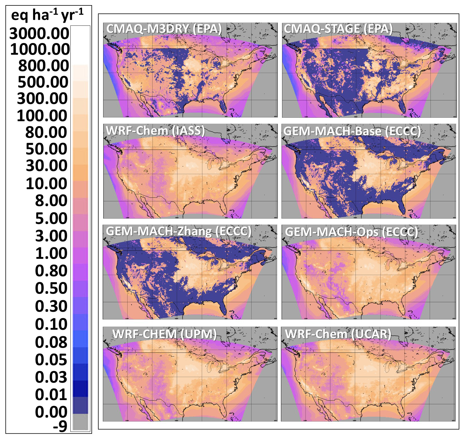
Figure 22 The 2016 N dry-deposition fluxes (eq. ha⁻¹ yr⁻¹) for NH₃(g) (eq. ha⁻¹ yr⁻¹). Note that regions outside the AQMEII4 common domain have been assigned an outside-domain mask value of −9.

The AQMEII4 diagnostics for NH₃ deposition provide further insight into the causes of the differences between the models employing NH₃ bidirectional fluxes. The most generic formula for NH₃ bidirectional fluxes is

$$\begin{array}{}\text{(5)}& F_T={\displaystyle \frac{c_{\mathrm{a}}-c_{\mathrm{c}}}{r_{\mathrm{sum}}}},\end{array}$$

where F_T is the net flux, c_a is the atmospheric concentration of ammonia gas, and r_sum is a sum of resistances associated with turbulent eddies and molecular diffusion of gaseous NH₃ across the reference height of air and the vegetation canopy. c_c is the canopy compensation point concentrations of ammonia gas at the top of the canopy and may be expressed as a function of the atmospheric concentration as well as compensation point concentrations near stomata and the ground (c_s,c_g) and of the aerodynamic resistance of ammonia gas (r_a). As can be seen from Eq. (5), if the atmospheric concentration is greater than the compensation point concentration, the flux will be positive (downward). If the atmospheric concentration is less than the compensation point concentration, the flux will be negative (upward). Galmarini et al. (2021, Appendix C) give the detailed formulae for the terms in Eq. (5), for the bidirectional flux models participating in AQMEII4. A comparison of r_a, r_sum, c_a, c_c, c_g, and c_s may thus provide insight into the differences between the predicted NH₃ dry-deposition fluxes for the models employing bidirectional flux parameterizations for the North American AQMEII4 ensemble. These terms were reported by AQMEII4 participants as the diurnal median (50th percentile) at each hour (UT) within each month. The median values for 16:00 UT (noon EDT) for July 2016 are shown in Fig. 23. It is important to note that the median values for a given hour (UT) may correspond to different days within a given month. For example, the median values of r_sum and r_a at 16:00 UT in July may not occur on the same day, and hence the median value of r_sum will not necessarily be greater than the median value of r_a, as might be expected from the equations governing the resistances as given in Appendix C of Galmarini et al. (2021). Also, not all models were able to report all variables (as noted above, for CMAQ-M3Dry, the net and ground compensation point concentrations were calculated offline of the model simulation and could not be included as AQMEII4 diagnostic parameters). However, substantial differences between the panels of Fig. 23 provide a useful indication of the relative importance of different pathways in the participating models.

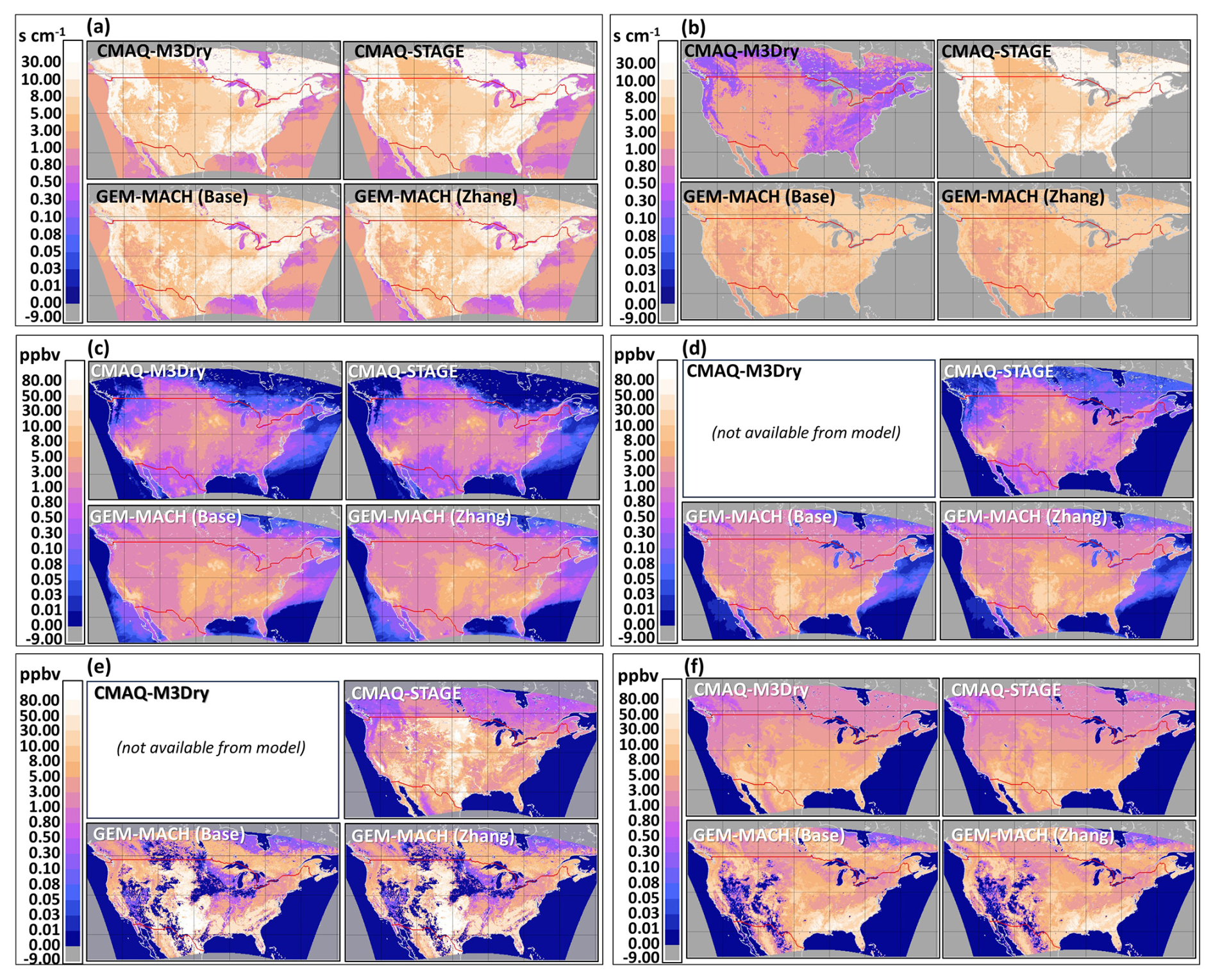
Figure 23 The 2016 spatial distribution from July 2016 at 16:00 UT with median N values for key bidirectional flux diagnostic variables. (a) Aerodynamic resistance (r_a; s cm⁻¹). (b) Sum resistance (r_sum; s cm⁻¹). (c) Air concentration of NH₃ (c_a; ppbv). (d) Net compensation point concentration (c_c; ppbv). (e) Ground compensation point concentration (c_g; ppbv). (f) Stomatal compensation point concentration (c_s; ppbv). Note that regions outside the AQMEII4 common domain have been assigned an outside-domain mask value of −9.

From Fig. 23, we note the following:

1. The median aerodynamic resistance r_a for July 2016 at 16:00 UT is similar for all four models (Fig. 23a); consequently, differences in r_a are unlikely to be the cause of the model flux differences.

2. The median r_sum values (Fig. 23b) for CMAQ-M3Dry for July 2016 at 16:00 UT is considerably smaller than for other models; at least some relatively high fluxes for CMAQ-M3Dry are due to these smaller r_sum values (which, appearing in the denominator for Eq. 5, will increase the magnitude of the fluxes).

3. The median r_sum values for CMAQ-STAGE over land for July 2016 at 16:00 UT are equal to those for r_a for this model. This is expected (r_sum=r_a for this model; Galmarini et al., 2021); other terms influence the magnitude and direction of the fluxes.

4. The median values of the air concentrations of NH₃ c_a (Fig. 23c) for July 2016 at 16:00 UT are lower for CMAQ-M3Dry and CMAQ-STAGE than for GEM-MACH (Base) and GEM-MACH (Zhang), as might be expected from the above-mentioned bias calculations relative to CrIS and AMoN data.

5. The median net compensation point concentration c_c (Fig. 23d) for CMAQ-STAGE for July 2016 at 16:00 UT is an order of magnitude smaller than for GEM-MACH (Base) and GEM-MACH (Zhang). From Eq. (5), this likely drives much of the large NH₃ flux for this model and its negative bias values; smaller c_c values will result in larger positive (downward) net fluxes F_T.

6. Some of the locations where CMAQ-STAGE's median ground compensation point concentration (c_g) for July 2016 at 16:00 UT maximized are where GEM-MACH (Base) and GEM-MACH (Zhang) have zero to near-zero ground compensation point values (Fig. 23e; e.g. Rocky Mountains, north-central US agricultural region; dark-blue areas in the GEM-MACH results compared to much lighter values in the CMAQ-STAGE results). The larger CMAQ-STAGE c_g values (local values were up to 1×10⁴ ppbv for this model), if dominant, would be expected to result in larger c_c values in Eq. (5) (see Galmarini et al., 2021) and hence a tendency towards smaller downward fluxes. This is not the case from the above analysis (DNH3 values in Table 5 for CMAQ-STAGE are greater than those of the GEM-MACH models, and CMAQ-STAGE NH₃ concentrations have more negative biases than the two GEM-MACH models), suggesting that the ground pathway is not the main term affecting the differences in model NH₃ dry-deposition fluxes.

7. For much of the AQMEII4 common domain (aside from the southwestern USA), CMAQ-M3Dry and CMAQ-STAGE have lower median stomatal compensation point concentrations for July 2016 at 16:00 UT than either GEM-MACH (Base) or GEM-MACH (Zhang) (Fig. 23f). This in turn implies that the difference in model dry-deposition fluxes is via the stomatal pathway.

The main factors resulting in higher-magnitude downward fluxes in CMAQ-M3Dry and CMAQ-STAGE relative to GEM-MACH (Base) and GEM-MACH (Zhang) are thus lower net compensation point concentrations (CMAQ-STAGE), lower stomatal compensation point concentrations (CMAQ-M3Dry, CMAQ-STAGE), and lower r_sum values (CMAQ-M3Dry).

All four bidirectional flux models calculate fluxes on specific land use types within each grid cell and use some form of land use fraction weighting to generate the values of the key parameters in the bidirectional flux equations. The native land use types used by each modelling platform were converted to a common set of 16 AQMEII4 land use types (see Galmarini et al., 2021). We investigated the CMAQ and GEM-MACH spatial and temporal patterns of ammonia bidirectional fluxes in the context of the AQMEII4 land use types, along with the relationship to the highest regions of nitrogen CLE. This is shown in Figs. 24 and 25, where Fig. 24a and b are the sum of AQMEII4 land use types 11 and 12 (i.e. the sum of the “planted/cultivated” and “grassland” land use types) used in CMAQ and GEM-MACH, respectively. Figure 24c and d are the sum of AQMEII4 land use fractions for land use types 6, 7, 8, and 13 (evergreen broadleaf forest, deciduous broadleaf forest, mixed forest, and savanna, respectively), for CMAQ and GEM-MACH, respectively. We note that these forested areas are the ecosystems of interest for many of the CLE values calculated earlier in this work. The land use summations of Fig. 25 are also worth noting in the context of the typical timing of the direction of NH₃ fluxes during the course of a day. Figure 25 shows an example of the diurnal behaviour of the NH₃ bidirectional fluxes for the CMAQ and GEM-MACH models, at (a) 15:00 CDT and (b) 07:00 CDT. Midafternoon fluxes (Fig. 26a) tended to be largely negative (upward; emissions; blue colours). However, the spatial location of the fluxes differs between the models even within a given model framework. CMAQ-M3Dry predicts afternoon emissions (blue colours) largely restricted to the combined grassland and agricultural land use types, with deposition (red colours) to the forested areas in southeastern Canada and the southeastern USA. CMAQ-STAGE predicts midafternoon emissions throughout western North America, though with a pattern of deposition similar to CMAQ-M3Dry in southeastern Canada and the southeastern USA. The GEM-MACH bidirectional fluxes in the afternoon are mostly negative (emissions; blue). All three models show midafternoon NH₃ deposition in the north-central USA, corresponding to a known region of high NH₃ concentrations (Fig. 21; CrIS NH₃ retrieval maximum). In contrast, early-morning fluxes (Fig. 25b) predicted by both CMAQ implementations are largely positive (downward; deposition; red colours), across all land use types, while GEM-MACH predicts deposition in agricultural areas and emissions further downwind in southeastern Canada and the southeastern USA.

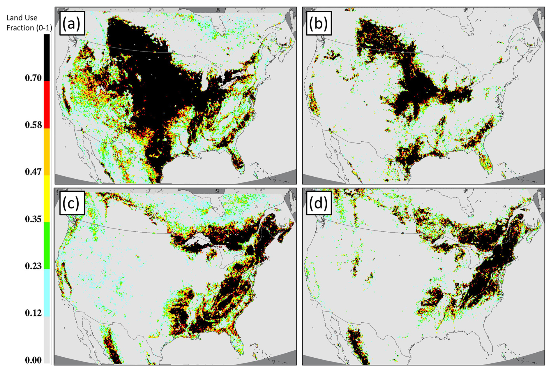
Figure 24 Comparison of AQMEII4 land use type fractions with locations of the highest CLE for forest ecosystems: CMAQ versus GEM-MACH. (a, b) Grid cell fractional area composed of the sum of AQMEII4 land use types 11 and 12 (planted/cultivated and grassland) for (a) CMAQ-M3Dry and CMAQ-STAGE and (b) GEM-MACH (Base) and GEM-MACH (Zhang). (c, d) Grid cell fractional area composed of the sum of AQMEII4 land use types 6, 7, 8, and 13 (evergreen broadleaf forest, deciduous broadleaf forest, mixed forest, and savanna) for (c) CMAQ-M3Dry and CMAQ-STAGE and (d) GEM-MACH (Base) and GEM-MACH (Zhang).

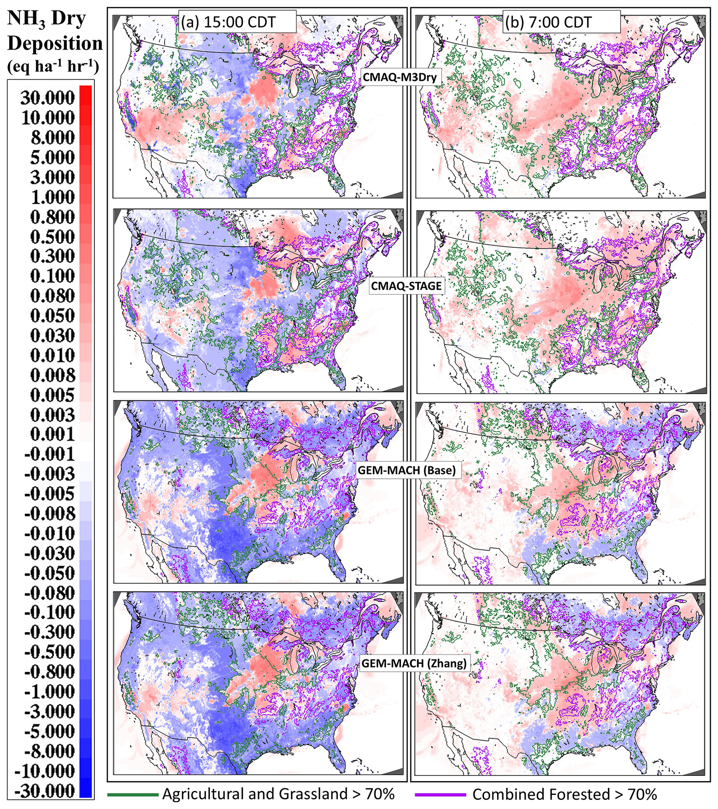
Figure 25 NH₃(g) flux (eq. ha⁻¹ h⁻¹) on (a) 4 August 2016 at 15:00 CDT and (b) 5 August 2016 at 07:00 CDT. Blue lines in the CMAQ and GEM-MACH model (horizontal row) panels enclose areas which are predominantly agricultural and grassland, whereas red lines enclose areas which are predominantly evergreen broadleaf forest, deciduous broadleaf forest, mixed forest, and savanna in each model's respective land use databases (see Fig. 24). Blue-shaded regions indicate negative (upward; emissions) NH₃ fluxes; red-shaded regions indicate positive (downward; deposition) NH₃ fluxes. Green lines show the boundary of regions where combined agricultural and grassland land use types comprise greater than 70 % of land cover. Purple lines show the boundary of regions where combined forest land use types comprise greater than 70 % of land cover.

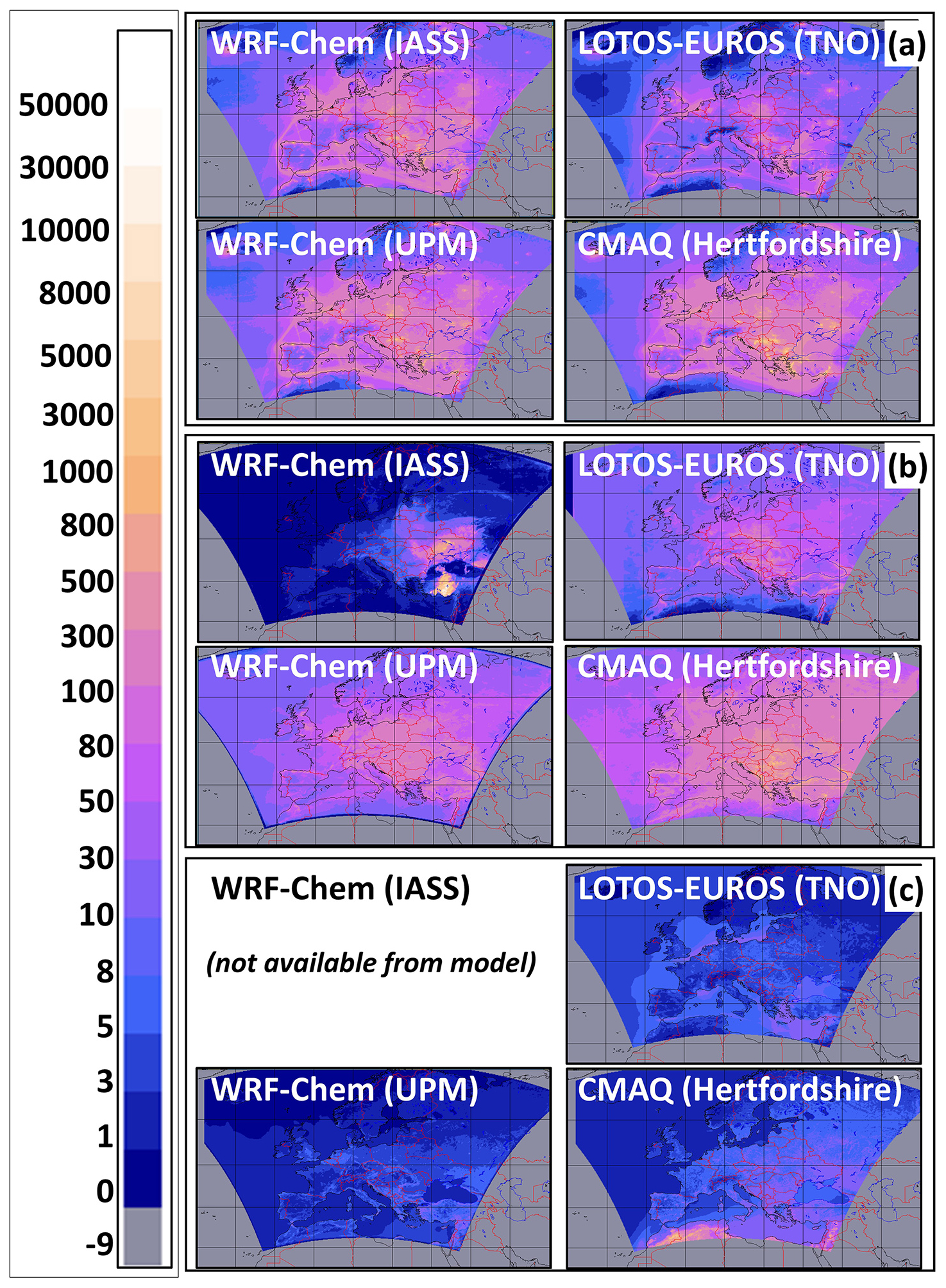
Figure 26 Spatial distribution and magnitude of contributions to annual S deposition, EU AQMEII4 common domain, 2010 (eq. ha⁻¹ yr⁻¹). (a) SO₂(g) dry deposition. (b) Total S wet deposition. (c) Particle sulfate dry deposition. Note that regions outside the AQMEII4 common domain have been assigned an outside-domain mask value of −9.

The generic diurnal sign changes in the direction of the ammonia flux across all four models is easily explained in reference to Eq. (5): in midafternoon (Fig. 25a), both the height of the planetary boundary layer and the magnitude of thermal coefficients of diffusivity are relatively high, reducing the ambient air concentration of ammonia gas (c_a in Eq. 5), resulting in negative fluxes (emissions; blue colours). In the early morning (Fig. 25b), both the boundary layer height and the magnitude of thermal coefficients of diffusivity are lower, hence increasing the ambient air concentrations of ammonia gas, resulting in more positive fluxes and prevalent deposition. However, the different bidirectional flux models show differences in diurnal behaviour by land use type. CMAQ-M3Dry and CMAQ-STAGE show a diurnal pattern of afternoon emissions from agricultural and grassland areas, deposition in forested regions downwind, and early-morning deposition irrespective of land use type. GEM-MACH shows stronger afternoon emissions regardless of land use type and morning lower-magnitude emissions in forested areas and deposition only in agricultural areas and the western USA.

We note that Table S4 measures model performance specifically at the satellite overpass time in the afternoon, i.e. at close to the time shown in Fig. 25a, and that the performance of CMAQ-M3Dry and CMAQ-STAGE is lower than the other models at this time, while the differences between the models aside from the magnitude of the bias is less pronounced in the integrated surface observations of Table S4. This analysis thus suggests that the CMAQ negative biases may be reduced in magnitude by re-examining the factors contributing to compensation point concentrations in forested areas in the day; c_c values (Eq. 5) are probably too low in these regions at these times, leading to excessive positive (downward) fluxes. That is, the analysis suggests that the CMAQ negative NH₃ biases may be the result of excessive deposition and/or insufficient emissions, in forested areas, in both the daytime and early morning, with the effect most noticeable in the afternoon. The bulk of the differences likely resides in the stomatal deposition pathway. Conversely, we note that the GEM-MACH bidirectional flux algorithm overestimates midafternoon ammonia in the southeastern USA relative to satellite observations (Fig. 21), indicating that compensation point concentrations may be overestimated in this region.

While NH₃ fluxes are only the fifth largest source of N deposition in the North American reduced ensemble, we also note that the manner in which NH₃ bidirectional fluxes are treated in the context of critical load exceedance calculations may be open to interpretation. Exceedances with respect to critical loads are calculated with respect to annual total deposition of N and S, but what constitutes total N deposition in the context of bidirectional fluxes is less clear. Here, we have taken the approach of assuming that negative fluxes (emissions) of NH₃ during the course of a year constitute a loss of N from the ecosystem but that NH₃ contained within the ecosystem cannot be converted to other forms of N. Consequently, the approach taken here was to sum the hourly NH₃ fluxes (positive downward and negative upward) for the year simulated, with only those grid cells with net positive summations (i.e. net annual deposition fluxes) adding to total N deposition. However, other interpretations are possible. For example, only the positive contributions on an hourly basis could be accumulated, and any losses of N from the same ecosystems associated with NH₃ emissions could be ignored/excluded from the N balance of the ecosystem. A third interpretation would be to assume that deposited NH₃ within the ecosystem may be converted to other forms of N, and hence the net NH₃ flux (which may be positive or negative in different parts of the region simulated) is added to N_dep, with N_dep being set to zero only when the NH₃ emission flux exceeds the deposition flux of all other forms of N. Here, we have taken the first of these approaches. We note that the second approach would lead to higher estimates of total N_dep than generated here, while the third approach would result in lower estimates of total N_dep. Although NH₃ is the fifth largest contributor to total N_dep across North America, these differences in approach may affect critical load exceedance estimates in regions of high NH₃ fluxes.

3.2.3 Causes of S deposition variability in European domain simulations

The relative contributions of the different sources of S deposition in the EU AQMEII4 common domain for the year 2010 are shown in Table 6 and Fig. 26.

The European ensemble contributions to total S deposition contrasted with those in North America; both the contribution to total S deposition and the magnitude of variability between the models follow the same descending order of importance: SO₂ dry deposition followed by (SO${}_{\mathrm{4}}^{\mathrm{2}-}$ + HSO${}_{\mathrm{3}}^{-}$) wet deposition, followed by particulate sulfate dry deposition (see Table 6). The relatively higher importance of SO₂ dry deposition to total sulfur deposition, compared to North America, may reflect a denser spatial distribution of SO₂ emissions in the EU domain compared to the North American domain, as well as higher EU emissions in 2010 compared to the NA 2016 year focused on here for model variability analysis. Another potential cause of differences between the two domains may reflect differences in the quality of the emission data (and emission reporting requirements) between the two jurisdictions. SO₂ emissions are largely from industrial stacks in both locations. In North America, regulations require that facility operators for large stack sources report their emissions and stack parameters making use of continuous emission monitoring, on an hourly basis (USA) or as annual reports (Canada). Plume rise algorithms may then be used to distribute the emissions in the vertical within air quality models. In the EU, stack sources are reported as annual totals without stack parameters which could be used for more accurate plume rise estimates (e.g. volume flow rates, effluent temperatures); the lack of these more detailed data necessitates approximations (either making use of “typical” plume rise rates or treating stack sources as surface emissions without plume rise). The larger variation in SO₂ performance in the simulations may thus reflect differences in the level of detail available within SO₂ emission inventories in the two regions.

European observation data for model evaluation were taken from the European Monitoring and Evaluation Programme (EMEP; https://www.emep.int/, last accessed 11 July 2024) and the European air quality database (AirBase; https://discomap.eea.europa.eu/map/fme/AirQualityExportAirBase.htm, last access: 3 March 2025.).

Table 6 Average S deposition contributions in the EU AQMEII4 common grid area (eq. ha⁻¹ yr⁻¹) and percent contribution to average total S deposition, 2010. n/d: no data. nr: not reported.

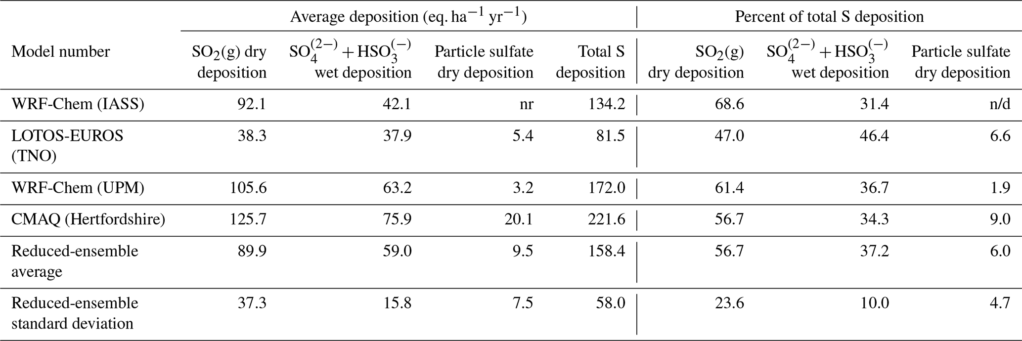
Dry deposition of SO₂

The model SO₂ performance metrics relative to observations at stations closer to urban centers (AirBase network) and more broadly distributed over the EU region (EMEP network), as well as comparisons to wet (SO${}_{\mathrm{4}}^{\mathrm{2}-}$ + HSO${}_{\mathrm{3}}^{-}$) deposition (EMEP wet-deposition network), are shown in Table S6 (Supplement). Observation station locations are shown in Fig. S17a. WRF-Chem (IASS) had the best SO₂ performance relative to both networks for most statistics, with the exceptions of a slightly smaller FAC2 score compared to other models for both AirBase and EMEP, and the largest negative bias for SO₂ relative to AirBase observations. The proximity of AirBase station locations to SO₂ sources can also be seen in Fig. 27, where the AirBase monthly concentration y axis (Fig. 27a) is almost twice that of the EMEP monthly concentration y axis (Fig. 27b). Observed SO₂ close to sources (Fig. 27a, red lines) shows a strong seasonal variability, with concentrations in the winter being a factor of 2 higher than in summer, likely showing the effect of increased winter stability on plume rise. This tendency is greatly reduced at regional stations (Fig. 27b, red lines). LOTOS-EUROS (TNO) matches the near-source SO₂ time series the most closely, while CMAQ (Hertfordshire) overestimates the impact of seasonal variability (Fig. 27a). At regional stations, LOTOS-EUROS (TNO) and CMAQ (Hertfordshire) overestimate seasonal variation, while WRF-Chem (IASS) most closely matches observations. At least some of the variation in the simulated SO₂ performance relative to observations and hence in SO₂ deposition fluxes and critical load exceedance estimates is due to some models overestimating the seasonal variation in SO₂ at regional locations further from cities. This may reflect differences in atmospheric stability, the seasonal response of the deposition algorithms, or the manner in which plume rise is simulated between the models.

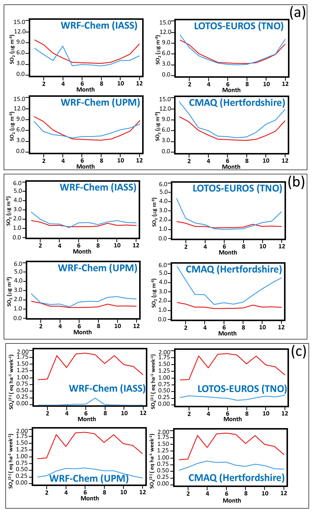
Figure 27 Comparison of observed and modelled S, EU AQMEII4 common domain, 2010. (a) AirBase SO₂ (µg m⁻³). (b) EMEP SO₂ (µg m⁻³). (c) Wet flux of total S deposition (eq. ha⁻¹ per week). Red: observations. Blue: model.

WRF-Chem (IASS) has the best overall performance for SO₂; while this model's mean bias is the most negative for observation sites close to the sources (AirBase comparison), the remaining statistics are the best of the ensemble, and the model bias performance is also better than the other models as the distance from the sources increases (EMEP comparison). The large negative biases in WRF-Chem (IASS) model values may indicate an overestimate of SO₂ deposition, though other model processes may also play a role.

Wet deposition of sulfur

As was the case for most models in the North American domain, all EU domain models underestimated wet deposition relative to observations (note negative biases in Table S6 and the monthly time series comparison versus observations in Fig. 27c). CMAQ (Hertfordshire) outperforms the other models relative to observations, though we note that the sulfur wet-deposition bias for this model is nevertheless −0.39 eq. ha⁻¹ yr⁻¹, with a correlation coefficient of 0.15. In contrast to the North American sulfur wet-deposition comparison time series (Fig. 15, Table S2), the European wet-deposition observations do not show a springtime peak in values, rather a seasonality centered around the month of June, with higher values extending from March to September.

None of the EU models made use of updated particle dry-deposition velocities available in more recent literature; as a result, the relative contribution of particle dry deposition to EU model-to-model variability is small. Speciated PM observations were not available for comparison to model predictions in the EU region.

Returning to the spatial distribution of the relative contributions of the three forms of sulfur deposition for the year 2010 shown in Fig. 26, CMAQ (Hertfordshire), with the highest SO₂ deposition flux (Fig. 26a; see also Tables 6, S6), also has the most positive SO₂ concentration mean bias. With increasing distance from the sources, the SO₂ loss or conversion processes of all four models are likely underestimated (EMEP SO₂ biases are positive for all models, Table S6). In contrast, all models have significant negative biases in sulfur wet deposition (Table S6); hence at least one reason for this underestimate may be insufficient conversion of SO₂ to ionic sulfate and bisulfite in simulated cloud water, through uptake of SO₂ and scavenging of particulate sulfate. The wet deposition of sulfur in WRF-Chem (IASS) in particular seems anomalously low (Figs. 26c, 27b), with much of Europe having little to no sulfate wet deposition in this model. A comparison of the relative differences in the deposition pathway strength for the models may help shed light on the causes of SO₂ deposition flux variability between the models. However, no effective fluxes were reported by LOTOS-EUROS (TNO). Figures S23 and S24 show the spatial distribution of the summed annual effective fluxes for the reporting models, with the results in the EU AQMEII4 common domain summarized in Fig. 28.

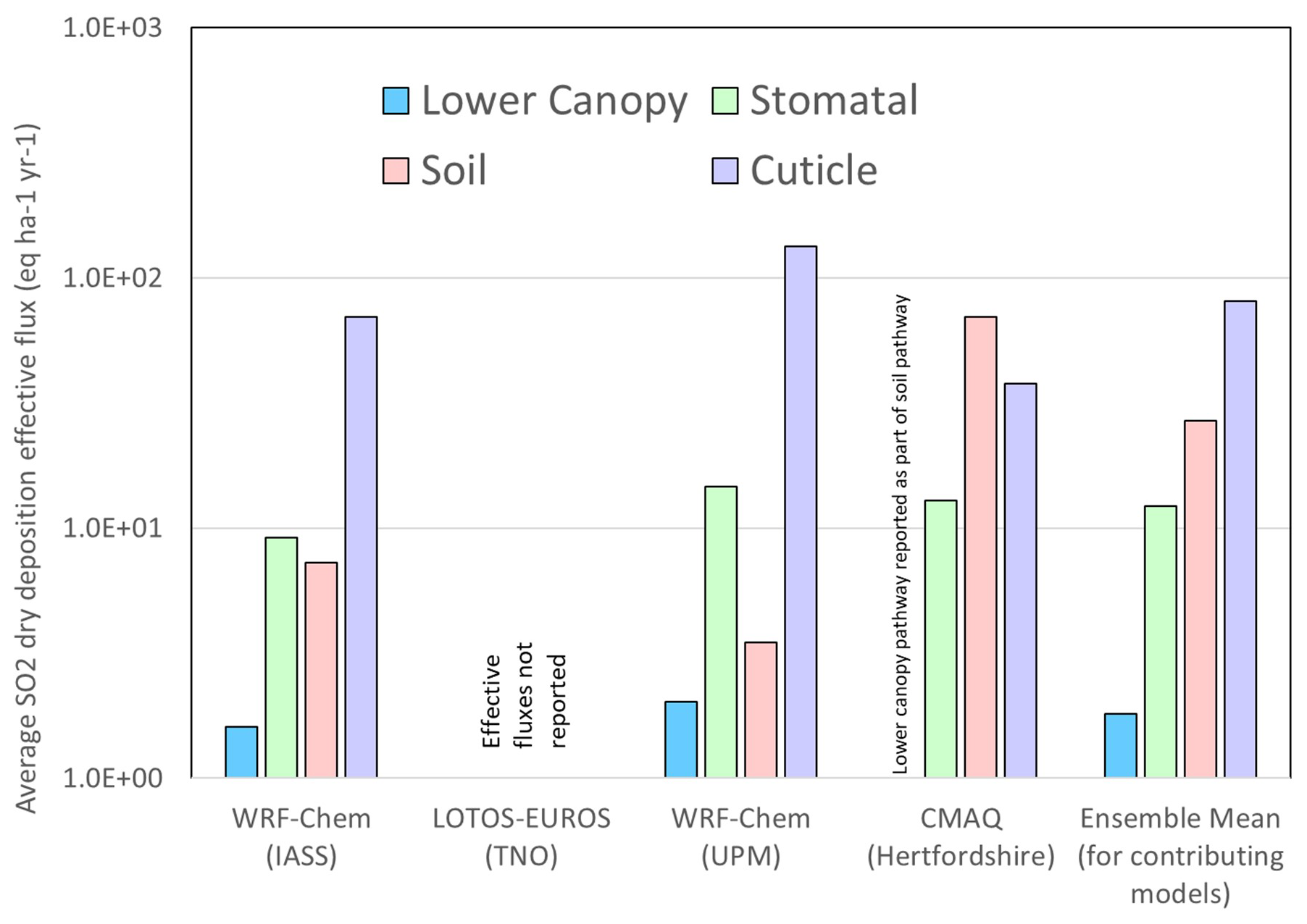
Figure 28 Averages of effective-flux pathway contributions to SO₂ dry deposition, EU AQMEII4 common grid, 2010 (eq. ha⁻¹ yr⁻¹).

Despite having the highest average SO₂ deposition flux (Table 6), CMAQ (Hertfordshire) also has the highest positive biases for SO₂ ambient concentrations (Table S6). From Figs. S23, S24, and 28, the CMAQ (Hertfordshire) positive biases may be the result of spatial variations in deposition, specifically, to low contributions to the cuticle effective fluxes in northern Europe for this model (Fig. S23a). Despite these relatively low values, the SO₂ net dry-deposition flux for this model (Table 6) is higher than that of the other models, implying that the low northern EU fluxes are being offset by higher values elsewhere (e.g. via the soil flux; compare soil and cuticle values in Fig. 28). We note that the effective-flux analysis is restricted to grid cells that do not have water as a dominant land use type (a maximum of 1 % water land fraction was used as an exclusion criterion); for grid cells held in common (mostly land), the CMAQ (Hertfordshire) the cuticle effective-flux pathway specifically is lower than that of the other models, while the differences are less noticeable for the other terms, as reflected by the summary values in Fig. 28. Other than northern Europe, CMAQ (Hertfordshire) has higher soil fluxes than WRF-Chem (IASS). Similar to AQMEII4 analyses for ozone (Hogrefe et al., 2025), the relative importance of the different pathways for total deposition varies between the models. For example, WRF-Chem (IASS), with the best overall performance for SO₂ concentrations aside from bias and factor of 2, has flux contributions in descending order of importance: cuticle, stomatal, soil, and lower canopy. For CMAQ (Hertfordshire), with relatively poor performance and high positive biases (Table S6), the flux contributions in descending order of importance are soil, cuticle, and stomatal (with the lower canopy being incorporated as part of soil flux, for this model), and the cuticle pathway contributes less to deposition in northern Europe than the other models.

3.2.4 Causes of N deposition variability in European domain simulations

The EU AQMEII4 common-domain relative contributions for each model's deposited species to total nitrogen deposition and its variability are shown in Table 7. The contributions to total N deposition for the reduced ensemble, in descending order of importance, were wet NO${}_{\mathrm{3}}^{-}$, dry HNO₃, wet NH${}_{\mathrm{4}}^{+}$, dry NH₃, dry particulate nitrate, dry NO₂, and dry particle ammonium, with relatively small contributions from the other depositing N species. The spatial distributions of the four largest contributions to total N deposition are shown in Fig. 29. The largest contributions to model-to-model variability, in descending order, were wet NO${}_{\mathrm{3}}^{-}$, dry HNO₃, dry NH₃, wet NH${}_{\mathrm{4}}^{+}$, and dry NO₂, with smaller contributions to variability from the other species.

Figure 29 Spatial distribution of contributions of (a) wet nitrate ion deposition, (b) dry gaseous HNO₃ deposition, (c) wet ammonium ion deposition, and (d) dry gaseous ammonia deposition to total N deposition in the EU AQMEII4 common domain, 2010 (eq. ha⁻¹ yr⁻¹). Note that regions outside the AQMEII4 common domain have been assigned an outside-domain mask value of −9.

Wet-deposition fluxes of NO${}_{\mathrm{3}}^{-}$ and NH${}_{\mathrm{4}}^{+}$ and the ground-level concentration of NO₂ are evaluated in Table S7 (Supplement); monthly average time series comparisons of wet deposition to the observations are provided in Fig. 30. From Fig. 29, WRF-Chem (IASS) predicted much lower-magnitude NO${}_{\mathrm{3}}^{-}$ wet-deposition and NH${}_{\mathrm{4}}^{+}$ wet-deposition fluxes than the other three models, and from Table S7, these result in larger negative biases and poor overall performance relative to observations for WRF-Chem (IASS) in comparison to the other models. LOTOS-EUROS (TNO) had the best overall performance for NH${}_{\mathrm{4}}^{+}$ and NO${}_{\mathrm{3}}^{-}$ wet-deposition fluxes. However, similar to the case for S wet deposition, all models have significant negative biases for both nitrogen ion wet fluxes, as can be seen from Table S7 and Fig. 30. LOTOS-EUROS (TNO) has the best performance for statistics relating to the spatial and temporal distribution of wet deposition, while WRF-Chem (UPM) has the lowest bias for NO${}_{\mathrm{3}}^{-}$ wet deposition. A common feature of the AQMEII4 ensemble of models for both EU and NA domains are these negative biases for wet deposition of both sulfate and nitrogen species. Also, we note that the observed NH${}_{\mathrm{4}}^{+}$ wet-deposition (Fig. 30b, red line) peaks in June, while the model values (blue lines) peak earlier, in March. This in contrast to the North American NH${}_{\mathrm{4}}^{+}$ comparison (Fig. 18), where observed peaks occur in April and model peaks occur in June.

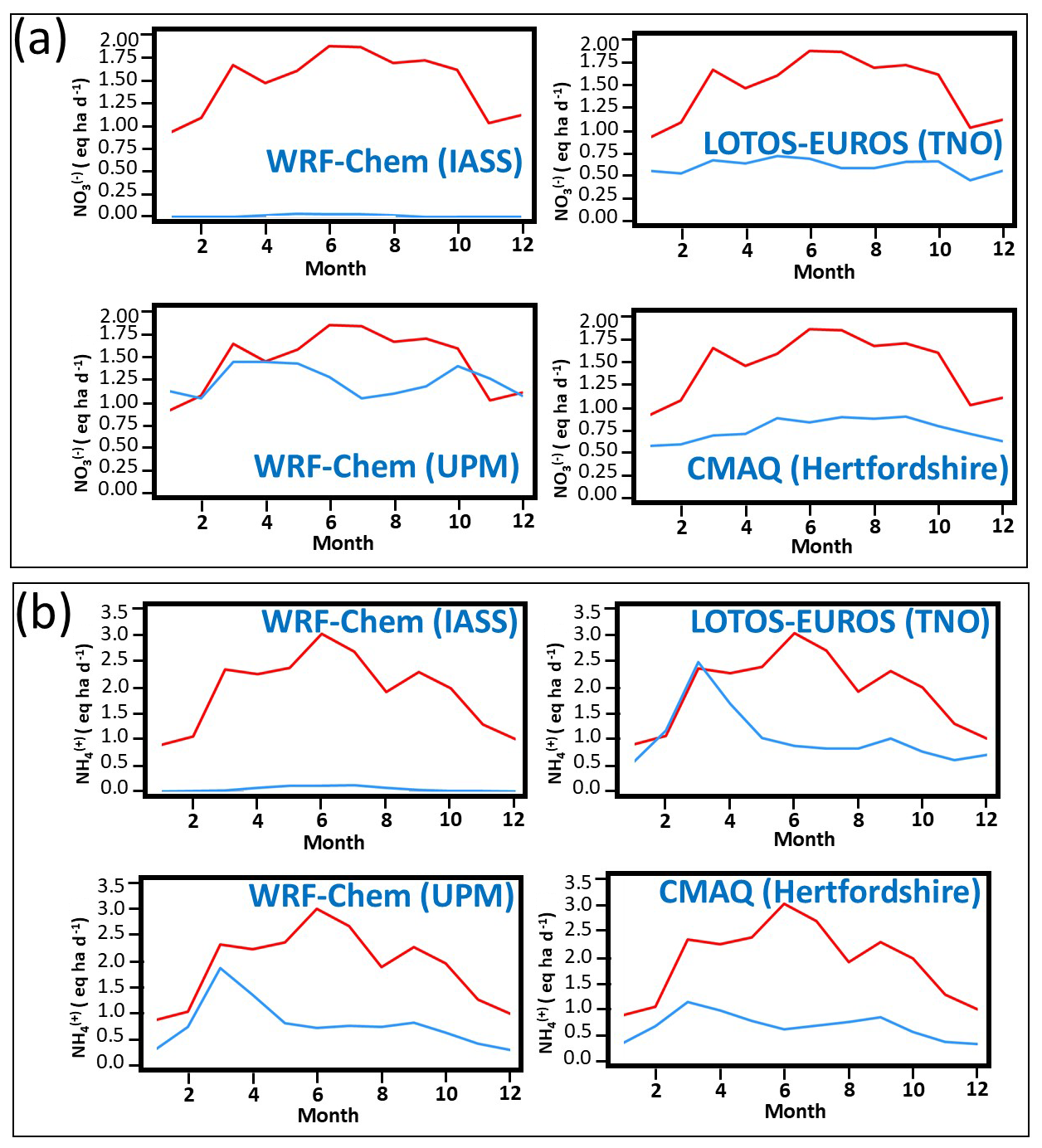
Figure 30 Monthly average comparison of nitrogen wet deposition, EU AQMEII4 common grid, 2010. (a) Average flux of NO${}_{\mathrm{3}}^{-}$(aq). (b) Average flux of NH${}_{\mathrm{4}}^{+}$(aq) (eq. ha⁻¹ d⁻¹).

Table 7 Contributions of N species to total deposition (eq. ha⁻¹ yr⁻¹) and percent of total N deposited, EU AQMEII4 common grid, 2010, arranged in descending order of importance to the reduced-ensemble average. DNH3: dry deposition of NH₃(g). WNH4: wet deposition of NH${}_{\mathrm{4}}^{+}$(aq). DHNO3: dry deposition of HNO₃(g). WNO3: wet deposition of NO${}_{\mathrm{3}}^{-}$(aq). DAM: dry deposition of particulate ammonium. DNI: dry deposition of particulate nitrate. DNO2: dry deposition of NO₂(g). DPAN: dry deposition of peroxyacetyl nitrate gas. DRN3: dry deposition of organic nitrate gases. DN2O5: dry deposition of N₂O₅(g). DHNO4: dry deposition of pernitric acid gas. DNO: dry deposition of NO(g). n/d: no data. nr: not reported. ndd: no dry deposition.

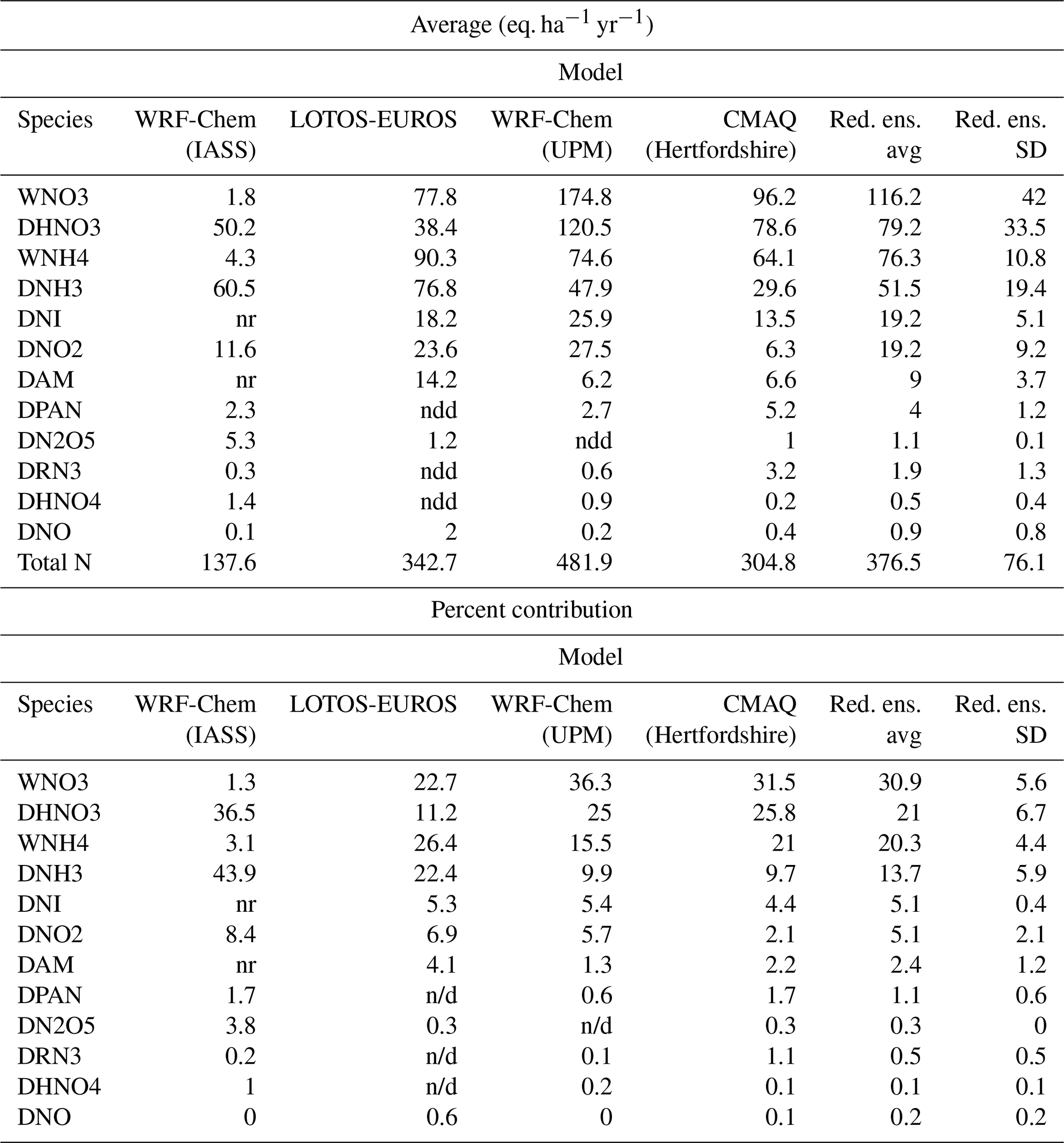
Dry deposition of HNO₃ was the second largest source of modelled EU nitrogen deposition variability. The spatial distribution of the relative contributions of the four pathways to the mass flux of HNO₃ is shown in Figs. S25 and S26 and is summarized for the entire grid in Fig. 31. There is more heterogeneity between the EU models regarding the relative importance of the HNO₃ deposition pathways than was observed for the North American simulations (compare Figs. 20 and 31). In the North American simulations, the cuticle deposition pathway also dominated for all models, followed by the soil pathways. In the EU simulations, the reported soil pathway for WRF-Chem (UPM) was several orders of magnitude smaller than the same pathway for CMAQ (Hertfordshire). The cuticle pathway dominated for WRF-Chem (IASS) (not shown) and CMAQ (Hertfordshire). The stomatal pathway magnitude is less than the cuticle pathway for the EU models but greater in general than for the North American models, where the stomatal pathway had a smaller contribution to HNO₃ dry deposition than the lower-canopy pathway.

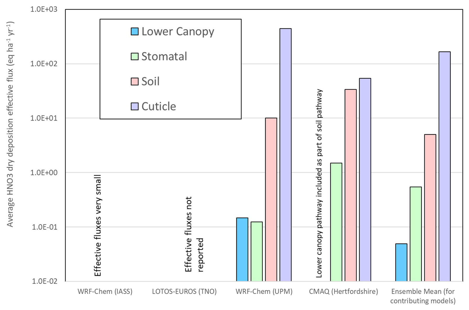
Figure 31 Averages of flux pathway contributions to HNO₃ dry deposition, EU AQMEII4 common grid, 2010 (eq. ha⁻¹ yr⁻¹).

Observations of 2010 HNO₃(g), NH₃(g), and dry particle nitrate were not available for comparison to the model predictions. However, observations of the NO₂ concentrations, the sixth largest contributor to total N deposition and the fifth largest contributor to model-to-model variability, were available at near-source AirBase and regionally distributed EMEP stations (Table S7). Aside from having the second largest-magnitude mean bias, LOTOS-EUROS (TNO) had the best performance for NO₂ relative to stations positioned close to emission sources (AirBase), while WRF-Chem (IASS) and CMAQ (Hertfordshire) had the best performance for NO₂ for stations distributed more widely across the region (EMEP).

4 Conclusions

We have used the AQMEII4 North American and European ensembles to calculate net sulfur and nitrogen deposition from individual models and a reduced ensemble of all models. These deposition estimates were used to calculate exceedances of critical loads for these two regions, using several critical load datasets. An in-depth analysis of the causes of model-to-model variability followed, using diagnostics designed for AQMEII4. We therefore subdivide these conclusions by the domain simulated, as well as the critical load exceedance and causes of model variability, within each domain.

4.1 North America: critical load exceedances

All simulations showed a decrease in the size of the area of exceedance and the severity of exceedances with respect to acidification of forest ecosystems and aquatic-ecosystem acidity between the years 2010 and 2016. The total area in exceedance for sensitive-epiphytic-lichen species richness improved slightly, but the severity of exceedance was greatly reduced. Given that the lichen community has a dose–response relationship with increasing deposition, this indicates reduced harm to forest health, even when the CL is still in exceedance. CLEs for herbaceous-species community richness had substantial improvements in the total area of exceedance and severity of exceedance. The amount of exceedance in any given year and the extent of reduction between the 2 years varied considerably between the models. Any individual model provided a similar direction of the change between the 2 years; the range of estimates suggests the utility of model ensembles where possible in estimating critical load exceedances, as well as model–measurement fusion, when sufficient S and N species data are available.

4.2 North America: causes of model S deposition variability

The total mass of North American sulfur deposition is as follows, in decreasing order of importance: wet deposition of S (SO${}_{\mathrm{4}}^{\mathrm{2}-}$ + HSO${}_{\mathrm{3}}^{-}$), dry deposition of particulate sulfate, and dry deposition of SO₂. Dry deposition of particulate sulfate contributed the most to model-to-model variability in total sulfur deposition, followed by wet deposition and dry SO₂ deposition. The models with the highest S wet-deposition levels had the best performance relative to monitoring network observations (CMAQ-M3Dry, CMAQ-STAGE, GEM-MACH (Ops)), though all models' S wet deposition was biased low relative to observations. A subgroup of models (GEM-MACH (Base), GEM-MACH (Zhang), GEM-MACH (Ops)) had the highest positive biases in observed PM_2.5 sulfate concentrations relative to monitoring network observations, contributing to the model-to-model variability. Recent work by Ryu and Min (2022) and Ghahreman et al. (2024) suggests that model negative biases for wet deposition may be improved through incorporation of multiphase hydrometeor scavenging, and this may also reduce positive biases in particulate mass resulting from the implementation of the Emerson et al. (2020) particle dry-deposition algorithm (GEM-MACH (Base) and GEM-MACH (Zhang)). Most North American reduced-ensemble models were in relatively good agreement with regards to their predictions for the total dry-deposition flux of SO₂(g).

4.3 North America: causes of N deposition variability

The largest contributors to the average total nitrogen deposition fluxes across North America in 2016 were wet ammonium ion, dry HNO₃, wet nitrate ion, dry particle ammonium, dry ammonia gas, dry particle nitrate, and dry NO₂, with relatively minor contributions from the other depositing gases. The largest contributors to the average total N deposition flux variability across models in descending order of importance were the deposition of dry particulate ammonium, wet ammonium ion, wet nitrate ion, dry nitric acid, dry particle nitrate, dry NO₂, and dry NH₃.

The first and second contributions to model-to-model variability between the members of the North American reduced ensemble were due to the three GEM-MACH implementations (Base, Zhang, and Ops) all having much higher particle ammonium dry-deposition and ammonium ion wet-deposition fluxes, zero to positive biases in ammonium ion wet deposition relative to observations during the summer, and the largest positive biases for PM_2.5 ammonium concentrations relative to observations, as a result of the simplified sulfate–ammonium–nitrate–water inorganic aerosol thermodynamics algorithm they employed. The positive biases in fine-mode particle ammonium concentrations and positive biases in ammonium ion wet deposition for this subgroup of models are likely caused by the absence of base cations as an alternative sink of nitric acid in addition to ammonium nitrate formation. Updates to these model implementations making use of a new, highly efficient solver for inorganic heterogeneous chemistry which includes the base cation reactions (Miller et al., 2024) should reduce these positive biases. The absence of multiphase hydrometeor scavenging of particle mass may also play a role in the particle ammonium positive biases for these models and in the negative biases across all North American models for ammonium wet deposition and nitrate wet deposition (Ghahreman et al., 2024).

Dry deposition of nitric acid was the second largest contributor to total nitrogen deposition fluxes in North America and the fourth largest contributor to model-to-model variability, with cuticle and the soil pathway dominating the HNO₃ mass flux, usually by more than an order of magnitude.

Comparisons of model-predicted 2016 concentrations of NH₃(g) to both CrIS satellite-based observations (in the afternoon, at overpass time) and ground-based AMON monitoring network values (biweekly averages) showed that the details of the implementation of ammonia bidirectional flux algorithms have a large impact on model NH₃ performance, with CMAQ-M3Dry and CMAQ-STAGE having the most negative NH₃ biases in NH₃ and GEM-MACH (Base) and GEM-MACH (Zhang) having the smallest-magnitude NH₃ biases. A detailed analysis of the magnitude and direction of these models employing bidirectional flux algorithms showed a common diurnal behaviour of daytime emissions from agricultural and grassland areas and deposition in downwind forested areas and nighttime deposition in all regions. However, the GEM-MACH models predicted low-magnitude net emissions from forested areas downwind of agricultural areas in the early morning, while the CMAQ models predicted net deposition at all locations. Differences in the relative magnitudes of compensation point concentrations and the strength of the daytime stomatal deposition pathway were shown to be the cause of these differences.

4.4 Europe: critical load exceedances

The AQMEII4 ensemble for Europe predicted similar exceedances with respect to acidity and eutrophication in 2009 and 2010, with the three-member reduced ensemble showing slightly reduced exceedance levels for acidity and slightly increased exceedance levels for eutrophication, in 2010. We note that the models used made use of inorganic aerosol thermodynamics algorithms which included reactions of base cations, and none made use of more recent updates to the particle dry-deposition parameterization (Emerson et al., 2020; Pleim et al., 2022). Consequently, the magnitude of differences between the models varied from the North American models, and the order of importance of different forms of sulfur to total deposition differed from the North American ensemble.

4.5 Europe: causes of model S deposition variability

The common-domain average reduced-ensemble sulfur dry-deposition contributions and their variability followed the same decreasing order of importance (SO_2,, wet S, dry particulate sulfate). WRF-Chem (IASS) had the best overall performance relative to observations for SO₂ concentrations, while CMAQ (Hertfordshire) had the best performance for S wet deposition. LOTOS-EUROS (TNO) and CMAQ (Hertfordshire) tended to overestimate regional SO₂ seasonality, with much higher concentrations in winter than summer compared to observations in the EMEP SO₂ network. Near-source observations (AirBase network) had higher winter than summer values, though this seasonal variation was largely absent in the observations for stations more representative of regional conditions (EMEP). The positive biases in modelled regional SO₂ concentrations for LOTOS-EUROS (TNO) and CMAQ (Hertfordshire) (the latter relative to both EMEP and AirBase stations) may reflect differences in plume rise distribution between the models or in their driving meteorology's vertical stability (e.g. the modelled wintertime atmosphere may be more stable than is observed, for these models). As was the case in the North American ensemble, all models had negative biases for S wet deposition. As in North America, the manner in which cloud scavenging of particulate sulfate and SO₂ was implemented in these models may be the cause of the wet-deposition negative biases. Unlike North America, speciated PM measurements were unavailable for model evaluation and bias correction.

EU SO₂ deposition pathways were investigated with AQMEII4 diagnostics; the soil and cuticle pathways dominated, and the stomatal pathway was relatively unimportant. This order of importance may reflect diurnal and seasonal SO₂ concentration variations. SO₂ concentrations are more likely to be high under more stable atmospheric conditions (these inhibit the rise in buoyant SO₂ plumes from large stack sources); these conditions are more likely to occur more frequently at night and in the winter, when the influence of the stomatal pathway is at its minimum.

4.6 Europe: causes of model N deposition variability

The relative contributions to total N deposition and the range in the EU domain were the following, in decreasing order of importance: wet nitrate ion, dry HNO₃, wet ammonium ion, dry ammonia gas, dry particle nitrate, and dry NO₂. The variations in the N deposition values between models were smaller than in North America, likely due to the use of base-cation-inclusive inorganic aerosol thermodynamic algorithms in all models and the use of older implementations of wet scavenging and particle dry deposition than in the North American models. We note that NH₃ dry deposition was the fourth largest contributor to European N deposition model-to-model variability, with the model employing a bidirectional flux algorithm (LOTOS-EUROS) having the highest NH₃ deposition. Satellite-based NH₃ data were unavailable for Europe for the years simulated but are recommended for simulation evaluation in more recent years.

LOTOS-EUROS (TNO) had the best overall performance for nitrate wet deposition, ammonium wet deposition, and near-source NO₂ concentrations compared to the other models. However, all EU models had substantial negative biases in nitrate and ammonium wet deposition, which is in common with the North American models. The seasonality of N wet deposition was poorly simulated, with most models failing to predict the observed summertime maximum of ammonium wet deposition. Given that this negative bias has its maximum in the summer, when agricultural NH₃ emissions are also likely to maximize, evaluation in more recent years of NH₃ predictions against satellite data is recommended.

In accordance with the NA ensemble, those EU models which reported effective-flux diagnostics for all four HNO₃ dry-deposition effective-flux pathways showed the cuticle and soil pathways dominating. The details of an individual land use database may be seen in the HNO₃ deposition flux diagnostics (Figs. S25 and S26), with differences in the amount of inland water being apparent. Furthermore, we note that the land use databases employed in critical load exceedance calculations may also differ from those used in individual models. Such mismatches are another source of uncertainty in the estimation the critical load exceedances for the dry-deposition portions of total S and N deposition. The effect of land use type classifications on model deposition fluxes for ozone will be examined in more detail in an upcoming paper (Hogrefe et al., 2025).

4.7 Impact of bias correction as a simple form of model–measurement fusion

A simple form of model–measurement fusion (bias correction) was applied to each of the models' species contributing to total sulfur and nitrogen deposition, for those component species for which observations were available, and corresponding bias-corrected critical load estimates were generated. This sometimes resulted in substantial decreases in model-to-model variability in the CLEs generated, indicating that model–measurement fusion will decrease model-to-model variability, as well as improved CLE estimates, provided sufficient data are available for the main contributors to total sulfur and total nitrogen deposition. In the case of Europe, the application of bias correction increased CLE variability for acidification, likely due to the lack of particulate sulfate observations in Europe for the years simulated. The substantial contrast to North American bias-corrected values suggests that the bias corrections for individual species contributing to total sulfur deposition may offset each other (e.g. positive biases in particle sulfate may be offset by negative biases in wet deposition). In the absence of speciated particle observation data in Europe, this compensating effect could not be captured using bias correction, and hence the European CLE variability increased with bias correction.

An important implication of the bias correction exercise conducted here is the need for observation data which close the sulfur and nitrogen deposition budgets to the greatest extent possible when carrying out model–measurement fusion. The biases with respect to observations for sulfur species may reflect inaccuracies in the transformation of one species to another, for example. If model–measurement fusion is applied to only some of the species contributing to sulfur deposition, the resulting total sulfur deposition field and exceedance estimates may be less accurate than the original model fields. Similarly, we note that the observations available here did not include particle nitrate or nitric acid data – and hence the impacts of model–measurement fusion on total nitrogen deposition may potentially lead to less accurate estimates than the original model values.

Recommendations: air quality modelling needs identified by the analysis.

Our analysis suggests that model biases and model-to-model variability may be reduced through targeted research into specific model process components. These include the following:

• multiphase hydrometeor scavenging of gases and aerosols into clouds to reduce the magnitude of wet deposition and particle concentration biases

• incorporation of improved particle deposition velocity algorithms (e.g. Emerson et al., 2020) – but only in combination with multiphase wet scavenging (Ryu and Min, 2022; Ghahreman et al., 2024)

• incorporation of base cation inorganic chemistry (if not already present) (Fountoukis and Nenes, 2007; Miller et al., 2024) and improved base cation emission inventory development

• NH₃ bidirectional fluxes evaluated using satellite data, with particular reference to improving compensation point estimates for forested areas

• land use type database harmonization across models and between models and critical load databases.