Identifying missing sources and reducing NO_x emissions uncertainty over China using daily satellite data and a mass-conserving method

This study applies a mass-conserving model-free analytical approach to daily observations on a grid-by-grid basis of NO₂ from the Tropospheric Monitoring Instrument (TROPOMI) to rapidly and flexibly quantify changing and emerging sources of NO_x emissions at high spatial and daily temporal resolution. The inverted NO_x emissions and optimized underlying ranges include quantification of the underlying atmospheric in situ processing, transport, and physics. The results are presented over three changing regions in China, including Shandong and Hubei, which are rapidly urbanizing and not frequently addressed in the global literature. The day-to-day and grid-by-grid emissions are found to be 1.96 ± 0.27 µg m⁻² s⁻¹ on pixels with available a priori values (1.94 µg m⁻² s⁻¹), while 1.22 ± 0.63 µg m⁻² s⁻¹ extra emissions are found on pixels in which the a priori inventory is lower than 0.3 µg m⁻² s⁻¹. Source attribution based on the thermodynamics of combustion temperature, atmospheric transport, and in situ atmospheric processing successfully identifies five different industrial source types. Emissions from these industrial sites adjacent to the Yangtze River are found to be 161. ± 68.9 Kt yr⁻¹ (163 % higher than the a priori), consistent with missing light and medium industries located along the river, contradicting previous studies attributing water as the source of NO_x emissions. Finally, the results reveal pixels with an uncertainty larger than day-to-day variability, providing quantitative information for placement of future monitoring stations. It is hoped that these findings will drive a new approach to top-down emissions estimates, in which emissions are quantified and updated continuously based consistently on remotely sensed measurements and associated uncertainties that actively reflect land-use changes and quantify misidentified emissions, while quantifying new datasets to inform the bottom-up emissions community.

1 Introduction

The sum of nitrogen oxide (NO) and nitrogen dioxide (NO₂), hereafter called NO_x, is produced during fossil fuel, biomass, and other combustion processes or from heat sources due to the re-combination of atmospheric N₂ and O₂ (Brewer et al., 1973; Logan, 1983). NO_x is a short-lived trace gas that directly impacts health, nitrate aerosols, tropospheric ozone (both an air pollutant and a greenhouse gas), and OH radicals, which indirectly impact both CO and CH₄ (Alcamo et al., 1995; Chen et al., 2007; Collins et al., 2013; Crutzen, 1970; Jacob et al., 1996; Li et al., 2018; Monks et al., 2015; Prather, 1996; Rigby et al., 2017; Rollins et al., 2012; Sand et al., 2016; Seinfeld, 1989; Shindell et al., 2012; Tan et al., 2018). Although there are techniques to observe in situ surface NO_x and the atmospheric column of NO₂ during the daytime via remote sensing in the ultraviolet (UV) and visible portions of the spectrum, there is no way to observe the atmospheric burden of column NO_x, and even observations of NO₂ during the nighttime are not reliable (Bauwens et al., 2020; Bechle et al., 2013; Boersma et al., 2009; Lamsal et al., 2014; Lee et al., 2014; Russell et al., 2011; van Geffen et al., 2020). Furthermore, due to rapid atmospheric chemistry, interactions with UV radiation, sensitivity to temperature and vertical structure, and pseudo-steady-state balance between NO₂ and NO, there is no simple way to quantify rapidly changing or emerging sources of NO_x emissions at high spatial and daily temporal resolution (Alvarado et al., 2010; Leue et al., 2001; Martin et al., 2003, 2006; Mijling et al., 2013).

Present approximations of NO_x emissions tend to miss emerging sources and underestimate sources undergoing rapid change while also overestimating highly regulated sources, leading to a combination of biases. These approximations also become rapidly outdated compared to rapid changes in emissions and economic structures, particularly in the Global South (Cohen and Wang, 2014; Dados and Connell, 2012; Lin et al., 2020; Qin et al., 2023; Wang et al., 2021; Zhu et al., 2014). Bottom-up aggregation uses a small subset of spatial and temporal measurements in the field or sometimes in the laboratory and combines these with economic, technological, and other data to scale up emissions (Amstel et al., 1999; Bond et al., 2004; European Commission Joint Research Centre, 2021; Li et al., 2017; Olivier et al., 1994; Oreggioni et al., 2021). This approach can also be applied to biomass burning emissions by including fire radiative power and other indirect remotely sensed measurements of land-use change, which are then scaled based on small spatial and temporal measurements of emissions factors, biomass, and other available data (Cohen et al., 2017; Giglio et al., 2013; van der Werf et al., 2017; Wang et al., 2020). Direct flux measurements can be made via a sparse network of local flux towers, each with a limited spatial range and operating under standard meteorological conditions (Geddes and Murphy, 2014; Haszpra et al., 2018; Karl et al., 2017; Lee et al., 2015). Chemical transport models can be merged with Bayesian, data assimilation, or Kalman filter approaches to invert emissions and produce error estimates, which in turn consume a huge amount of computational time and require explicit knowledge of the errors of every input variable, including those in the modeling system itself (Cohen and Wang, 2014; Henderson et al., 2012; Napelenok et al., 2008). There have even been some direct inversions of results from isolated and very strong, non-time-varying sources, which require these sources to be surrounded by clean background conditions and apply the very strict assumptions of Gaussian plume modeling (Beirle et al., 2011, 2019; Cohen and Prinn, 2011; De Foy et al., 2014; Jin et al., 2021; Laughner and Cohen, 2019) or integrate data over a long and continuous period of time, over a specific season, or with another set of conditions that generally remains unchanged and then assumes a fit of the average spatial and temporal emissions (Kong et al., 2022).

Although the above methods have their own advantages, there are still significant problems, including missing sources, underapproximation of small and moderate sources (Beirle et al., 2021; Drysdale et al., 2022; Qin et al., 2023), underestimation of the spatial and temporal variability of sources with large variability (Stavrakou et al., 2016; Vaughan et al., 2016; Wang et al., 2010; Zyrichidou et al., 2015), and the inability to scale a priori regions with zero emissions (Cohen, 2014; Zhao and Wang, 2009). In general, these methods do not provide an uncertainty analysis, or they require model and measurement uncertainty to be highly parameterized (Bond et al., 2013; Cohen and Wang, 2014). There is no reason why NO_x emissions should be static in time or have a constant ratio of NO to NO₂, even though these are current assumptions which are built into most models used by the community (Li et al., 2023b). This combination of weaknesses has limited most emissions studies to scaling-based perturbations of NO_x emissions, without considering the spatial and temporal variation in the distribution, therefore requiring the implicit adaptation of large spatial and temporal averages (Evangeliou et al., 2018; Lund et al., 2020; Wang et al., 2021). This, in turn, tends to miss significant emissions sources from rapidly changing sources such as wildfires, sources including new urbanization, and sources which are changing due to changes in the climate system itself (Deng et al., 2021).

This work applies the recently introduced mass-conserving model-free approximation of NO_x emissions (MCMFE-NO_x) approach, using daily-scale remotely sensed tropospheric columns of NO₂ from the Tropospheric Monitoring Instrument (TROPOMI) at native resolution with a spatial resolution of 3.5 km × 7 km, which was subsequently reduced to 3.5 km × 5.5 km in August 2019, in combination with reanalysis wind fields to approximate the daily NO_x emissions and uncertainty ranges over major population and economic regions of greater China (China and its Special Administrative Regions). The specific results herein are applied to robustly account for the uncertainties in the remotely sensed column observations of NO₂ and actively provide a quantification of the range of thermodynamics driving the ratio of NO to NO₂, dynamical transport, and a first-order in situ chemical loss, all within the context of the tropospheric column measurement and a priori emissions uncertainty ranges. This approach allows for non-linear feedbacks to be accounted for, including those from climate-induced changes to policy-induced changes, some of which are analyzed in the context of the results provided. The modeling was done on a PC and is model independent, allowing the results to be rapidly reproduced; improved upon with updated measurements and physical, chemical, and other routines; and integrated rapidly into all existing modeling and policy frameworks, with little to no additional computational cost (Cohen et al., 2011; Cohen and Prinn, 2011; Holmes et al., 2013; Prinn, 2013).

In this work, MCMFE-NO_x is applied over three rapidly changing regions (Fig. 1) in China with densely urbanized sub-regions and surrounding rural regions, rapidly developing suburban and urbanizing sub-regions, and new developments aiming to upgrade urban areas and energy-intensive industries in these areas to meet the large-scale developmental and climate goals set by the Chinese national government (Bao, 2018). Detailed emissions estimates are made using 1 year of daily TROPOMI NO₂ data. Unlike the vast majority of air pollution emissions studies, which focus on the three large and well-characterized locations of Beijing–Tianjin–Hebei, the Yangtze River Delta, and the Pearl River Delta (Haas and Ban, 2014; Wang et al., 2022; Yang et al., 2021), the estimates specifically include adjacent areas, which include large cities with overall populations similar to or larger than the previously studies areas, including Wuhan along the middle Yangtze River; Qingdao, Jinan, and other cities in Shandong Province; and Shantou and Xiamen along the South China Sea. In addition, rapidly industrializing locations that have previously not been included, such as Zibo, Ma'anshan, and Beihai, are now included. The estimates also include highly developed cities such as Beijing, Shanghai, and Hong Kong SAR (which has never had gridded a priori emissions developed in the past by either the Multi-resolution Emission Inventory for China (MEIC) or EDGAR); cities which have recently reached highly developed status but have undergone a large number of recent changes, including Nanjing, Suzhou, Dongguan, and Foshan; heavily coal-based and oil-based resource regions such as Tianjin and Tangshan; industrial cities including Xuzhou; and agricultural areas such as Jining, Heze, Meizhou, and Xinyang (Cai et al., 2019; Chang and Kim, 1994; Dhakal, 2009; Liu et al., 2021; Wu, 2016; Zhang et al., 2008; Zhuang et al., 2022). The large amount of variability of sources, rapid economic development, and strong changes in environmental emissions policy and regulation have led to significant changes in terms of emissions magnitude, in both space and time, over this region (Carson et al., 1997; Charfeddine and Kahia, 2019). Traditionally, NO_x emissions from water bodies have been regarded as negligible. Some findings have reported that NO_x emission from lakes is due to several biological and microbial processes (Kong et al., 2023). Other findings have only considered that the contribution of NO_x emissions over water must be attributed to shipping activities (Zhang et al., 2023). However, in this work, NO_x emissions and underlying forcing properties inverted day by day at a 0.05° × 0.05° grid resolution clearly point to the fact that there are missing small- and medium-sized power plants and industrial facilities that play an essential role and can also produce significant emissions, which these other studies have overlooked. The co-location along the edges of water bodies is in part due to the fact that these sites can both use the water for cooling purposes and possibly transport incoming and/or outgoing raw material and products.

2 Data and methods

2.1 Geographic boundaries of study region

In the realm of published air pollution research in China, most scholarly work has concentrated on three different regions: Beijing and surrounding areas, Shanghai and surrounding areas, and Guangzhou and surrounding areas. The first of these regions is usually defined as encompassing Beijing, Tianjin, and Hebei. In this work, we instead opted for an approach based on the column loading climatology of NO₂ as well as industrial and population density, as displayed in Fig. 1. First, since it is observed that NO₂ loadings in Hebei and near the Great Wall in northern Beijing are relatively low north of 40.5°, this work places a boundary here. Other regions are identified in which the column NO₂ with a climatology smaller than 1.43×10¹⁵ molec. cm⁻² is also excluded. The goal is to delineate a boundary along a contiguous contour of a high-NO₂ climatological loading, implying that the data needed to compute the emissions will be more clear and less influenced by observational noise. Our proposed continuous region 1 encompasses a substantial portion of adjacent Shandong Province to the south and east, which is known to have a high population density and extensive mineral, oil, and heavy manufacturing enterprises. The eastward extent ends in Qingdao (with a population of 9.5 million people and considerable manufacturing and ports). To the south, the region extends into the far end of northern Jiangsu Province, encompassing the cities of Xuzhou (with a population of 8.8 million people and considerable moderately intensive industry) and Lianyungang (one of the largest ports in China). We used a similar approach to extend the region commonly used around Shanghai to match with the observed climatological loadings of NO₂. The new area extends far up the Yangtze River to the west and now includes the city of Wuhan (with a population of more than 9.1 million (and growing) and considerable industry). Additionally, there are new locations in between that are identified and included, which are characterized by burgeoning coal utilization or energy infrastructure, as well as rapid population and industrial development. The region has nearly doubled/tripled in size by including the continuous region west from Nanjing and Hangzhou all the way through Wuhan, as displayed in Fig. 1. Similarly, the typical regions in the south have been extended beyond Guangzhou to Shenzhen and other adjacent cities in the Pearl River Delta. The new region includes substantial urban, financial, and commercial centers such as Hong Kong and Xiamen, which have previously been excluded. Similarly, other industrial cities and port cities, such as Beihai and Shantou, are also included. These cities, now stretching along the South China Sea continuously from the Vietnamese border to the East China Sea, provide a broader perspective on the geographical scope of our research and account for the unique characteristics of the Asian monsoon in a consistent manner (Cohen, 2014; Ding et al., 2021; Wang et al., 2021).

Figure 1 A map of the three study regions, including the names and locations of 30 important cities mentioned in this work.

2.2 TROPOMI tropospheric NO₂ column retrievals

The Sentinel-5 Precursor satellite from the European Space Agency is equipped with an advanced instrument known as the Tropospheric Monitoring Instrument (TROPOMI) (van Geffen et al., 2020; Veefkind et al., 2012), which is a nadir-viewing spectrometer with an overpass time of approximately 13:30 LST. The TROPOMI spectrometer measures ultraviolet (UV), visible, and near-infrared spectral bands and allows for observation of NO₂ and other air pollutants, aerosols, and clouds. TROPOMI measures NO₂ vertical columns with a spatial resolution of 3.5×7 km² (reduced to 3.5×5.5 km² since August 2019) and with a swath width of ∼ 2600 km.

The research herein uses the reprocessed dataset S5P-PAL, version 2.3.1, and includes all days with data from 1 January to 31 December 2019. The selection of the year 2019 is based on its status as the first complete year of NO₂ retrievals by Sentinel-5P. To ensure data quality, only pixels with a “qa_value” of 0.75 or higher are utilized. This pixel filter, which is recommended for most users, excludes cloud-covered scenes (cloud radiance fraction > 0.5), portions of scenes covered by snow or ice, errors, and problematic retrievals (https://data-portal.s5p-pal.com, last access: 11 July 2023) (van Geffen et al., 2022). As shown in Fig. 2a and b, the pixels of NO₂ column observations within each swath are amalgamated into unified latitude–longitude grids measuring 0.05° × 0.05° in size, using the weighted polygon-shaped remotely sensed measurement toolkit HARP (http://stcorp.github.io/harp/doc/html/index.html, last access: 4 February 2025). An area-weighted average is performed, ensuring that the re-gridded values accurately represent the spatial distribution of the original data (http://stcorp.github.io/harp/doc/html/algorithms/regridding.html, last access: 4 February 2025).

2.3 A priori emissions inventory

The assumptions regarding NO_x emission datasets in the initial step applied are harmonized using multi-source heterogenous data developed by the Multi-resolution Emission Inventory for China (MEIC) team (Huang et al., 2012, 2021; Kang et al., 2016; Liu et al., 2016; Zheng et al., 2021; Zhou et al., 2017, 2021) in collaboration with various scientific research institutions. This dataset is referred to as the high-resolution INTegrated emission inventory of Air pollutants for China (INTAC), which is highlighted in purple in Fig. 3. The original INTAC emissions are quantified in units of megagrams per grid per month, with a temporal resolution of 1 month and a spatial resolution of 0.1° × 0.1° for the year 2017. It is important to note that a higher-spatial-resolution inventory, the 1 km resolution by MEIC, is also available (Zheng et al., 2021). However, this 1 km inventory only offers one data point per grid per year while also providing insight into emissions from 2013, which in China are quite different from those in 2019. For this reason, we used INTAC since it more closely matches the 2019 TROPOMI data. This dataset covers mainland China and includes emissions from eight sectors: power, industry, residential, transportation, agriculture, solvent use, shipping, and open biomass burning (Wu et al., 2024). To align the resolution of the original INTAC with that of TROPOMI grids, we undertake several processing steps. (1) The units are converted from megagrams per grid per month to µg m⁻² s⁻¹ as the first step due to the varying areas of each latitude–longitude grid. (2) Next, INTAC is adjusted to a 0.05° × 0.05° grid using the nearest-neighbor method. (3) Finally, we assume that the monthly emissions remain constant on a day-to-day basis. To ensure that the values used do not fall within the error range of the TROPOMI sensor (i.e., noise), values below 0.2 µg m⁻² s⁻¹ are designated as NaN and are not considered further in this study.

2.4 Wind data

The parameters of wind speed and direction are used from ERA5 reanalysis (Hersbach et al., 2018, 2020). To correspond with the overpass timing of TROPOMI, this study employs the average value of the u and v wind products, recorded hourly at 05:00 and 06:00 UTC. The specific product used is taken at a spatial resolution of 0.25° × 0.25° to facilitate a more accurate representation of the atmospheric column conditions (https://www.ecmwf.int/en/forecasts/dataset/ecmwf-reanalysis-v5, last access: 4 February 2025) and is subsequently interpolated onto the same TROPOMI 0.05° × 0.05° grid in space and time. Since many of the areas considered in this work are low-lying urban conglomerates, with most of the terrain situated below an elevation of 500 m, wind data at the 950 hPa level were selected.

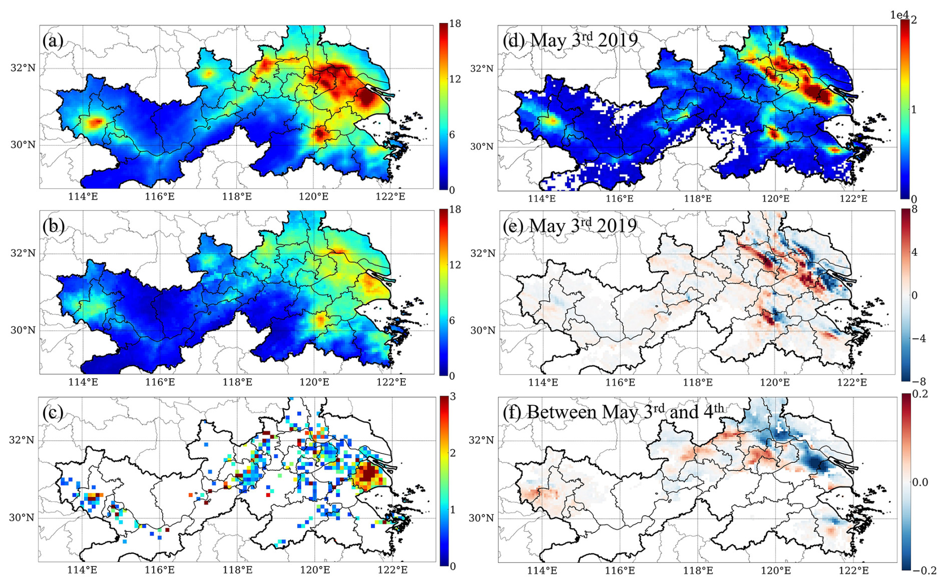
Figure 2 (a) TROPOMI daily climatology of NO₂ column loading (10¹⁵ molec. cm⁻²), (b) standard deviation (SD) of daily NO₂ column loading (10¹⁵ molec. cm⁻²), (c) INTAC monthly climatology of NO_x emissions (µg m⁻² s⁻¹), (d) TROPOMI NO₂ column loading (µg m⁻²) on 3 May 2019, (e) gradient of wind multiplied by TROPOMI NO₂ column loading (µg m⁻² s⁻¹) on 3 May 2019, and (f) the temporal derivative of TROPOMI NO₂ column loading between 3 and 4 May (µg m⁻² s⁻¹).

2.5 Inverse model

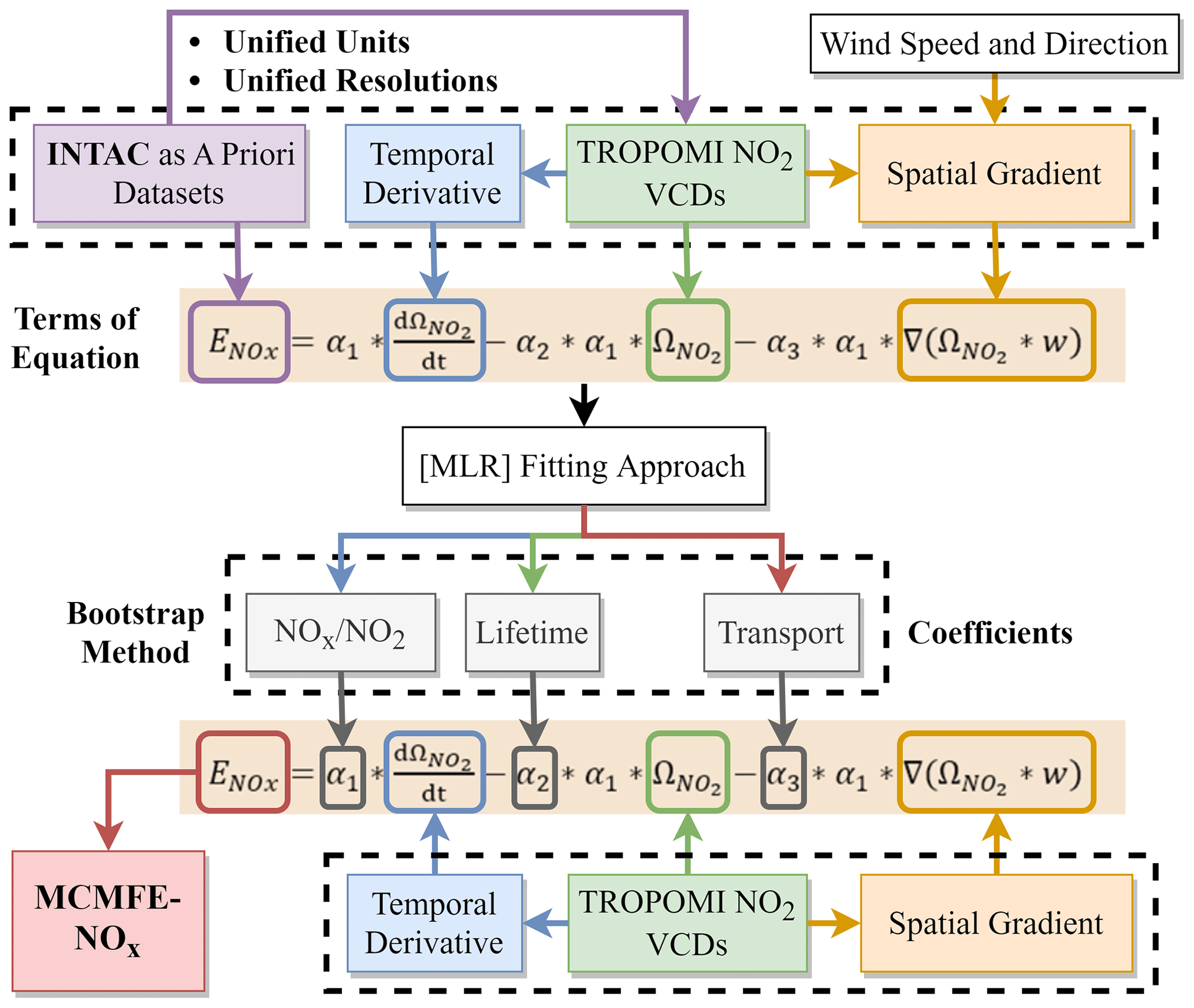
This study develops a flexible model based on first-order physics, chemistry, and thermodynamics and the continuity equation (mass conservation of trace species in the atmosphere) to approximate the emissions of NO_x as shown in Fig. 3 (Li et al., 2023a; Qin et al., 2023). Given a set of chemical substances in the atmosphere $(i=\mathrm{1},\mathrm{\dots }n)$ with molar fractions (or mixing ratios) C_i, the vector $C=(C_{\mathrm{1}},\mathrm{\dots }{C}_n{)}^T$ can be solved for based on conservation of mass in a fixed Eulerian reference system, following Eq. (1), where v is the 2-D wind vector, P_i and L_i are the production and losses of i (which may include contributions from species), E_i is emissions, and D_i is the sum of wet and dry deposition.

$$\begin{array}{}\text{(1)}& {\displaystyle \frac{\partial C_i}{\partial t}}=-\mathrm{\nabla }\cdot \left(v{C}_i\right)+P_i\left(C\right)-L_i\left(C\right)+E_i-D_i(i=\mathrm{1},\mathrm{\dots }n)\end{array}$$

The local rate of change in the column loading with time ($\partial C_i/\partial t$) is expressed as the sum of the input minus the output of the transport (i.e., gradient transport v⋅∇C_i and pressure transport C⋅∇v_i) and the net local output ($P_i\left(C\right)-L_i\left(C\right)+E_i-D_i)$. Note that in the case that the wind field is non-divergent, the gradient term ∇⋅(vC_i) reduces to term v∇C_i (Sun, 2022). In this work, the chemical substances C_i are generalized as TROPOMI NO₂ VCDs, which are denoted as ${\mathrm{\Omega }}_{{\mathrm{NO}}_{\mathrm{2}}}$. The rate of change in ${\mathrm{\Omega }}_{{\mathrm{NO}}_{\mathrm{2}}}$ in the troposphere can be determined by a balance between emissions, chemical/physical losses, and transport of the two individual terms NO and NO₂ by assuming that at the time of emission they are related to each other by the ratio ${\mathrm{NO}}_x={\mathit{\alpha }}_{\mathrm{1}}\cdot {\mathrm{NO}}_{\mathrm{2}}$ and then retaining α₁ as one of the terms to be flexibly solved for later in order to ensure that the model fits the observations from TROPOMI and INTAC. According to Eq. (1), and approximating the chemical loss as first order with a lifetime of $\mathrm{1}/{\mathit{\alpha }}_{\mathrm{2}}$ and the transport factors as linear with a distance of $\mathrm{1}/{\mathit{\alpha }}_{\mathrm{3}}$, the following mathematical model (2) can be constructed, where the emissions of NO_x are denoted as $E_{{\mathrm{NO}}_x}$. The terms are then rearranged to solve for the emissions in Eq. (3).

$$\begin{array}{}\text{(2)}& {\displaystyle }\begin{array}{rl}{\displaystyle \frac{\mathrm{d}\left({\mathit{\alpha }}_{\mathrm{1}}\cdot {\mathrm{\Omega }}_{{\mathrm{NO}}_{\mathrm{2}}}\right)}{\mathrm{d}t}}& =E_{{\mathrm{NO}}_x}+{\mathit{\alpha }}_{\mathrm{2}}\cdot \left({\mathit{\alpha }}_{\mathrm{1}}\cdot {\mathrm{\Omega }}_{{\mathrm{NO}}_{\mathrm{2}}}\right)+{\mathit{\alpha }}_{\mathrm{3}}\\ & \cdot \mathrm{\nabla }\left(\left({\mathit{\alpha }}_{\mathrm{1}}\cdot {\mathrm{\Omega }}_{{\mathrm{NO}}_{\mathrm{2}}}\right)\cdot v\right)\end{array}\text{(3)}& {\displaystyle }\begin{array}{rl}{E}_{{\mathrm{NO}}_x}& ={\mathit{\alpha }}_{\mathrm{1}}{\displaystyle \frac{\mathrm{d}\left({\mathrm{\Omega }}_{{\mathrm{NO}}_{\mathrm{2}}}\right)}{\mathrm{d}t}}-{\mathit{\alpha }}_{\mathrm{2}}{\mathit{\alpha }}_{\mathrm{1}}\cdot {\mathrm{\Omega }}_{{\mathrm{NO}}_{\mathrm{2}}}-{\mathit{\alpha }}_{\mathrm{3}}{\mathit{\alpha }}_{\mathrm{1}}\\ & \cdot \mathrm{\nabla }\left({\mathrm{\Omega }}_{{\mathrm{NO}}_{\mathrm{2}}}\cdot v\right)\end{array}\end{array}$$

The daily TROPOMI NO₂ columns, monthly INTAC emissions, daily temporal derivative, and spatial gradient computed and utilized to fit the terms α₁, α₂, and α₃ in Eq. 3 are shown in Fig. 2c–f.

The first term in the Eq. (3) symbolizes the influence of the rate of change in NO₂ columns on the estimation of NO_x emissions; more simply put, if the concentration is higher on the second day, then there must have been an emissions source larger than all other factors in balance, and if the concentration is lower on the second day, then there must have been sinks larger than the emissions source. Here, α₁ illustrates the linear ratio of NO₂ to NO_x and is a function of the thermodynamics of combustion when NO and NO₂ are first formed, as well as in situ atmospheric thermodynamics and rapid chemical adjustment after the combusted plume is lofted into the air. There is a basis for the use of α₁, which varies in space and time from both a chemical engineering perspective (Le Bris et al., 2007; Schwerdt, 2006) and an observational perspective (Karl et al., 2023). The formation of thermal nitrogen oxides (NO_x) is a process characterized by the reaction of atmospheric nitrogen (N₂) with atmospheric oxygen (O₂) under high-temperature conditions, and the NO_x-to-NO₂ process rapidly achieves a local pseudo-steady-state equilibrium. The formation of NO₂ and nitric oxide (NO) is significantly influenced by thermal conditions. NO is preferentially formed at temperatures exceeding 1200°; when the temperature surpasses 1100°, thermal NO_x becomes the predominant contributor to overall NO_x emissions, reaching a peak when the temperature exceeds 1600°. The secondary term α₂ in the equation signifies the physical and chemical production and destruction of NO_x, which are intrinsically associated with the chemical lifetime of NO_x. Finally, the third term introduces the concept of horizontal-flux divergence, denoted by α₃, representing the advective- and pressure-induced atmospheric transport of NO_x.

In this work, the divergence is computed using a second-order central difference method. The terms α₁, α₂, and α₃ are fit month by month and grid by grid (at 0.05° × 0.05°) when and where data are available (including INTAC) using multiple least squares regression (MLR). Certain extreme values of α₁, α₂, and α₃ are mathematically computed but are not physically plausible and are discarded from further consideration in these cases. In particular, grids exhibiting a ${\mathrm{NO}}_x/{\mathrm{NO}}_{\mathrm{2}}$ ratio less than 1 and a positive chemical loss term or chemical lifetime of NO_x less than 30 min are designated as NaN. Subsequently, in each month and on each grid, α₁ is sampled over 10 000 times within the 20th and 80th percentiles of the computed probability density function (PDF). For grids which already have fitted values of α₁, α₂, and α₃, in any given month, the bootstrap method is not applied, and the fitted values are used for each day in that given grid. If the grid does not have α₁, α₂, and α₃ or if it does but not during the month being used, then the bootstrap method will still be used to compute the emissions and uncertainty range.

On a daily and grid-by-grid basis where there is TROPOMI NO₂ column data and wind data and the temporal derivative and spatial gradient are computable, the following bootstrap method is used to compute the emission and the uncertainty range. First, the distributions of α₁ and the corresponding α₂ and α₃ from the same month at all points in the region are resampled 1000 times per grid. Using the resampled coefficients, the model given in Eq. (3) is finally used to compute the emissions of NO_x on a grid-by-grid and month-by-month basis. The mean of each grid-by-grid distribution of the runs is hereafter assigned as the mean emissions, while the standard deviation of each grid-by-grid distribution of the runs is hereafter assigned as the range of emissions uncertainty in that grid and on that day.

Figure 3 The framework of the mass-conserving approach (MCMFE-NO_x).

2.6 Location of sources

An important objective of this study is to analyze the emission and thermodynamic characteristics of various emission sources. To achieve this, the location data of five different high-energy-use facilities, which operate under different power, thermodynamic, and other conditions including power plants, steel and iron industries, heat production and supply, cement factories, and biomass burning, are selected as the input parameters for the distribution calculations. The location data of each of these types are obtained from the Pollutant Discharge Permit Management Information Platform of the Ministry of Ecology and Environment (http://permit.mee.gov.cn, last access: 4 February 2025), which contains information on these emission sources (name, city, latitude, and longitude). It is important to note that not all these sources are of sufficient scale to be equipped with continuous emission monitoring systems (CEMSs) for emissions monitoring. Many of these sources are small- to medium-sized industries, which do emit pollutant gases such as NO_x and have applied for formal discharge permits. The location data enable us to correlate satellite observations with identified emission sources, thereby providing valuable insights into emission patterns and their thermodynamic characteristics.

3 Results and discussion

3.1 Driving factors

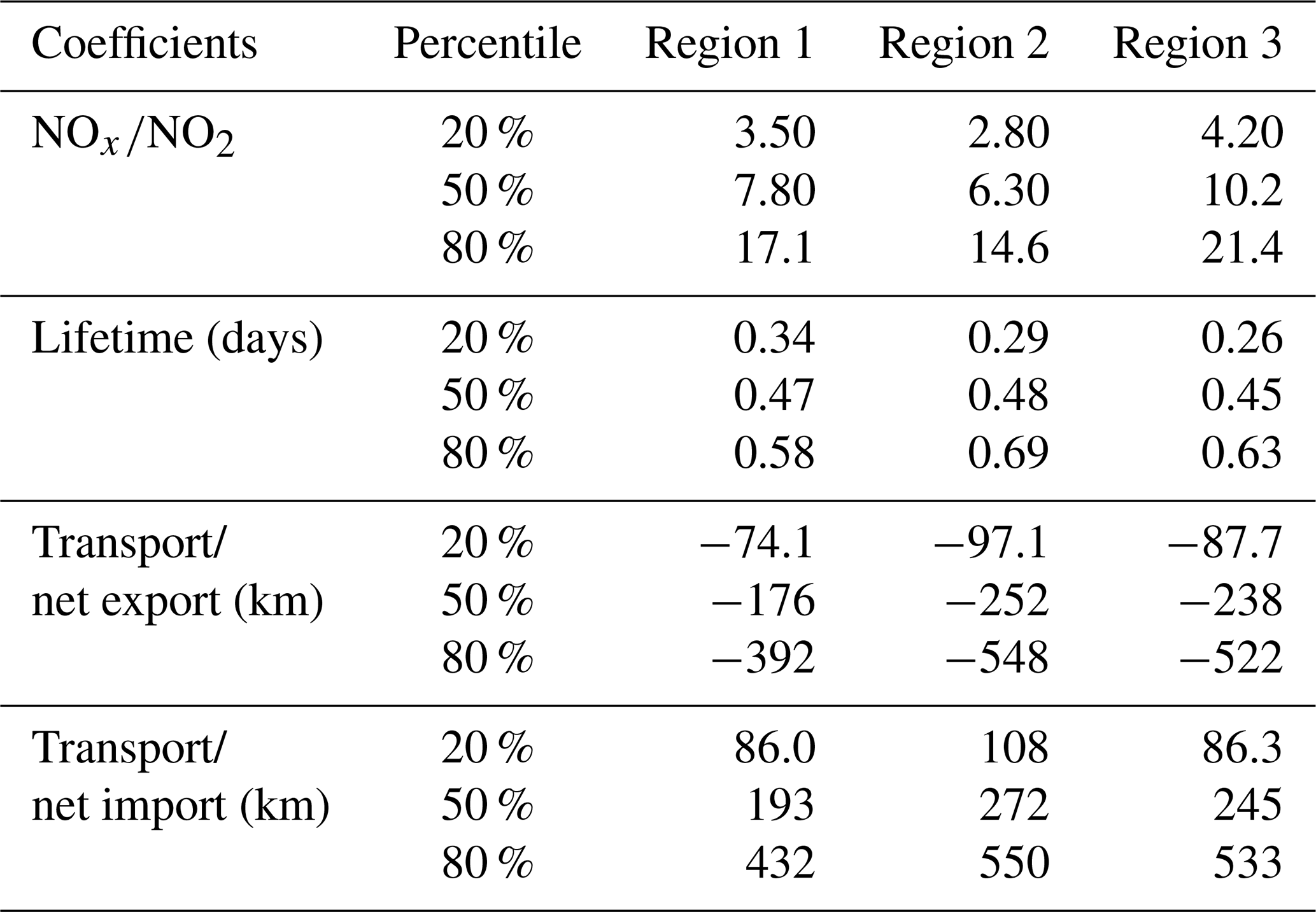
To examine the robustness of the coefficient results to the choice of study regions, the results obtained from the urban areas Suzhou, Nanjing, and Shanghai are resampled and refitted between the original fit's 20th and 80th percentiles, and the results of the updated statistical distribution of monthly α₁ values are compared with the original distribution. The resulting distributions of ${\mathrm{NO}}_x/{\mathrm{NO}}_{\mathrm{2}}$ (α₁), lifetime (related to α₂), and transport distances (related to α₃) (Table 1) over the two cases are nearly identical, demonstrating the stability of the MLR fitting method when used in connection with the emissions model, the physical constraints employed on the fitted values, and sampling the 20th to 80th percentiles. Unlike existing models that offer limited ranges (Beirle et al., 2019), this work accommodates higher variability and conforms to empirical observations (Karl et al., 2023; Laughner and Cohen, 2019). The annual percentiles from 20 % to 80 % for α₁ values in regions 1, 2, and 3 are observed to be within the intervals of 3.9 to 19.0, 2.9 to 15.0, and 4.4 to 22.2, respectively, while the lifetimes are within intervals of 0.34 to 0.60, 0.28 to 0.67, and 0.25 to 0.62 d, respectively. Overall, the community has assumed that negative transport (or net export from highly emitting boxes) dominates the transport. It has generally been assumed that emissions exit from an urban area, and the impacts of upwind sources entering the background of an urban area or source are frequently not considered. However, the results herein show that this is only the case 55 %, 49 %, and 54 % of the time over the three domains, respectively. This means that a significant amount of mass is transported into emitting areas from upwind emitting areas and is consistent with the computed positive transport (net import) values of 45 %, 51 %, and 46 %. There are some theoretical studies and case studies which have demonstrated that this is the case, but none have used observations over such a long time period to analyze the frequency of occurrence (Cohen et al., 2011; Cohen and Prinn, 2011; Wang et al., 2023).

The sensitivity of the fitted coefficients (α₁, α₂, and α₃) remains relatively robust to the changes in the a priori NO_x emissions. We design a perturbation run in which the emissions are randomly altered day by day and grid by grid from the a priori dataset near the extreme upper and lower bounds of their ± 30 % uncertainty range. This is then used in combination with the original values from TROPOMI to refit the coefficients, as given in Table S1 and Fig. S1 in the Supplement. It is observed that over 60 % of the grids of the ${\mathrm{NO}}_x/{\mathrm{NO}}_{\mathrm{2}}$ ratios and lifetimes and 40 % of the grids in terms of the transport terms are found to be robust, i.e., have a change smaller than the 30 % perturbed a priori emissions.

Table 1 Ranges of ${\mathrm{NO}}_x/{\mathrm{NO}}_{\mathrm{2}}$, lifetime, and transport distances computed from an annual dataset at 20 %, 50 %, and 80 % from region 1, region 2, and region 3, respectively.

The monthly distributions of ${\mathrm{NO}}_x/{\mathrm{NO}}_{\mathrm{2}}$ (α₁) and lifetime across various grids are presented in Fig. 4a–c. The parameter α₁, as observed across all three research areas, demonstrates a peak in July and August, a minimum in December and January, a second peak in February in the mean, and 60th percentile and 80th percentile cases and does not follow a standard seasonal pattern. When looking at α₁ on a region-by-region basis, the underlying factors become clearer. Regions 1 and 2 exhibit an α₁ value that is relatively consistent with the overall pattern described above, with the only difference being region 1 has a secondary peak in February, while region 2 does not. In these cases, the pattern is closely related to both the atmospheric temperature and the demand for excess power for heating as the centralized systems in the north of the country do not shut off until early March. Region 3 records a markedly elevated monthly α₁ compared to the other regions from October to April, with a second overall annual peak during March at the 80th percentile and during April at the 20th percentile. This is again consistent with the atmospheric temperature experienced in the Asian monsoon region and the extreme extra energy required for air conditioning during the dry and hot times that occur annually from February to April, frequently rivaling those of the summer when it is more cloudy and rains more. An important final finding is that the mean value of α₁ is biased and always found to be in between the 60th and 80th percentiles.

With respect to the lifetime of NO_x, the month-to-month value and variability of the mean and 60th percentile are similar to each other, while the variabilities of the 20th, 40th, and 80th percentiles are all larger. At the 20th percentile, November and December experience a longer lifetime than the rest of the year, consistent with reduced UV radiation. February deviates from the other months, consistent with economic and energy demands as well as emissions overall being very different during the Chinese New Year period. In particular, the 80th percentile lifetime has the longest annual value, while the 20th and 40th percentiles have the shortest annual values, indicating that high spatial and temporal variability exists in the emissions response to the movement of 500–800 million people over the annual 2-week-long holiday. Similarly, the mean value of lifetime is found to be biased between the respective 60th and 80th percentile values.

Additionally, Fig. 4d presents the mean ${\mathrm{NO}}_x/{\mathrm{NO}}_{\mathrm{2}}$ values of various cities. The lowest values, consistent with few to no industrial sources and high levels of vehicle and residential use, are found in Wuxi and Macau SAR, respectively, both of which are known as high-GDP and low-energy-intensive production cities and both of which are economically advanced. The next tier levels are observed in well-known urban areas like Beijing, Nanjing, Suzhou, and Hangzhou, which are similarly economically advanced and have high levels of car usage and public transportation but also have some factories and industry. The next tier is found in places like Shanghai, Qingdao, Hong Kong, Nanjing, and Wuhan, which are similar to the tier above but also combine significant sources related to shipping and co-related industries, including refining and other heavier industries. The highest values are found in Heze, Lianyungang, and Beihai, all of which have a large amount of heavy industry, coal- and oil-based industries for both energy and materials production, large ports, and other energy-inefficient sources, as well as lower overall vehicle penetration rates and a rapidly growing economy. It is interesting to note that there are some exceptions, such as Ma'anshan, which is lower than expected, since it is economically similar to Heze, Lianyungang, and Beihai and has a considerable coal industry. Moreover, this location also has a large amount of biomass burning to clear agricultural waste.

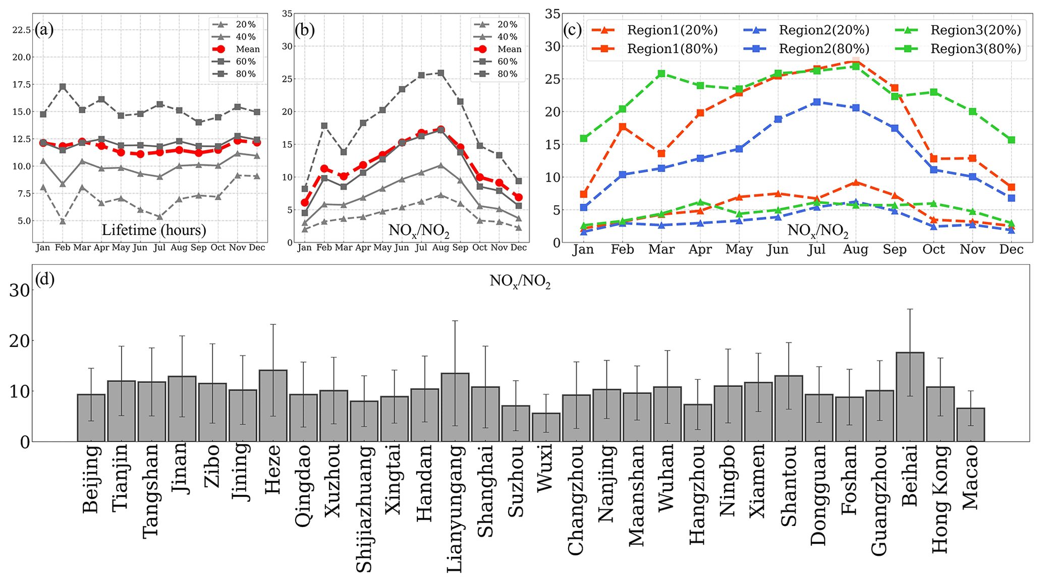
Figure 4 The distribution (mean values and 20th, 40th, 60th, and 80th percentile values) of monthly (a) lifetime, (b) ${\mathrm{NO}}_x/{\mathrm{NO}}_{\mathrm{2}}$, and 20th and 80th percentile values of monthly (c) ${\mathrm{NO}}_x/{\mathrm{NO}}_{\mathrm{2}}$ in the three regions and (d) mean values of ${\mathrm{NO}}_x/{\mathrm{NO}}_{\mathrm{2}}$ over 30 cities.

This work analyses the measurements and distributions of ${\mathrm{NO}}_x/{\mathrm{NO}}_{\mathrm{2}}$ over five different identified industrial source types: power plants, steel and iron factories, cement factories, heat production and supply, and biomass burning. The spatial distribution of the five emission source types and their temporal median ${\mathrm{NO}}_x/{\mathrm{NO}}_{\mathrm{2}}$ values in region 1 are presented in Fig. S2, with the statistics of grids within different ranges of ${\mathrm{NO}}_x/{\mathrm{NO}}_{\mathrm{2}}$ given in Table S2. The proportion of grids with α₁ values exceeding 10 continues to exhibit a distinct difference between three groups: steel and iron factories (up to 52 %); power plants (intermediate values, about 40 %); and cement factories, heat production and supply, and biomass burning (lower values). Even though the emissions rapidly adjust to the hot air emitted at the stack or pipe exit, this is clearly significantly influenced by the thermodynamics of combustion itself and additional factors including NO_x control technologies (LNB and SCR), combustion technologies (related to heat rates and efficiency), and local policies. These results clearly demonstrate that the original thermodynamic conditions still significantly influence the ${\mathrm{NO}}_x/{\mathrm{NO}}_{\mathrm{2}}$ values at the scale observed by TROPOMI. The rationale for this analysis is that each of these types of combustion sources has very different set combustion temperatures, oxygen availability, and other properties. Through both monthly distributions (Fig. 5a–e) and annual analysis of the PDFs of α₁ values (Fig. 5g–k), it is clearly demonstrated that α₁ has a significantly different set of characteristics across the different sources.

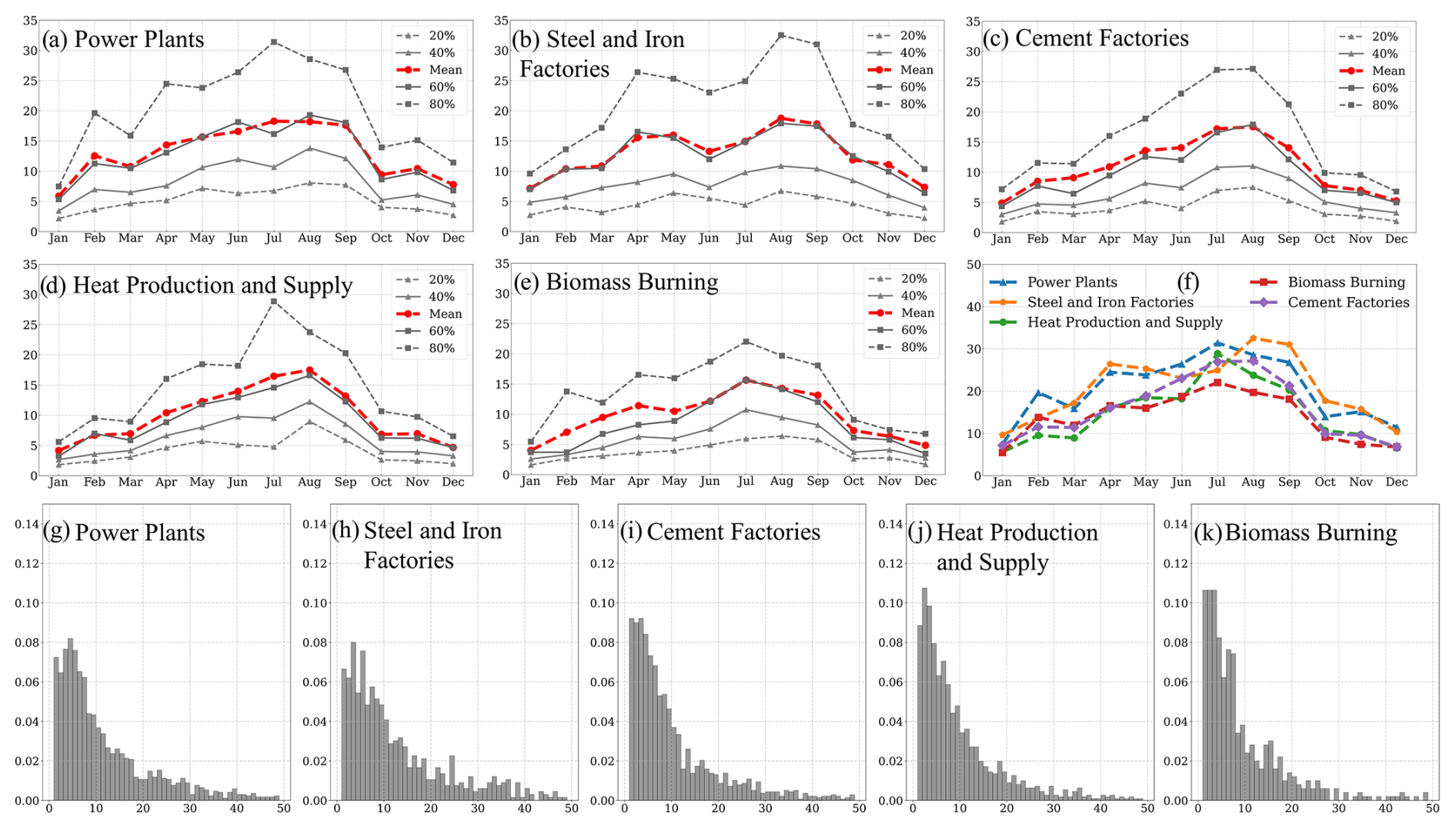
Figure 5 The distribution (mean values and 20th, 40th, 60th, and 80th percentile values) of monthly ${\mathrm{NO}}_{\mathrm{x}}/{\mathrm{NO}}_{\mathrm{2}}$ over grids from different sources: (a) power plants, (b) steel and iron factories, (c) cement factories, (d) heat production and supply, (e) and biomass burning, as well as the distribution of the 80th percentile values of (f) each source and (g)–(k) the PDFs of annual ${\mathrm{NO}}_x/{\mathrm{NO}}_{\mathrm{2}}$ of each source.

Table 2 Ranges of ${\mathrm{NO}}_x/{\mathrm{NO}}_{\mathrm{2}}$ from five different industrial source types at 10 %, 20 %, 50 %, 80 %, 90 %, and a high–low ratio (hl_ratio), hereafter defined as (90 %–80 %) $/$ (20 %–10 %). Attribution is achieved in terms of the 50th percentile factor and hl_ratio factor, given in the right column.

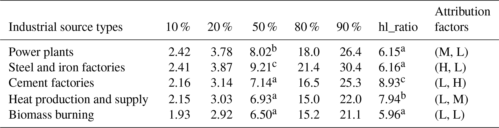
^a Low (L) values, ^b medium (M) values, and ^c high (H) values.

Thermal power plants primarily focus on electricity generation, with the maximum operational temperature reaching up to 2000° and steel and iron factories utilizing blast furnaces operated at high flame temperatures ranging from 1350 to 2000°. As a result, the ${\mathrm{NO}}_x/{\mathrm{NO}}_{\mathrm{2}}$ computed over the grids encompassing the two high-temperature sources is noticeably higher when compared to other sources. The monthly values of steel and iron factories are slightly less stable (more variable) than those of power plants. In the uppermost ranges (80th and 90th) of the PDF, the values corresponding to steel and iron factories exceed those of power plants and other sources, likely due to the extremely high temperatures used in the production of certain high-grade stainless steel. The manufacturing of cement involves combustion in a clinker at around 1000°C for preheating and in a precycled tower at around 1400°C to complete the process of chemical reaction. Therefore, while the values from cement factories are generally relatively high but lower than those of the power plants and steel factories, they favor NO₂ during part of the process and NO during a different part of the process. As expected, it is found that the values of α₁ for cement are lower than those of power plants and steel and iron factories but higher than those of the other source types. Heat production and supply generate steam and hot water through boilers and other devices and export heated water and steam. These are similar to power plants but operate at a lower temperature and efficiency. Accordingly, this factor also has relatively low α₁ values in each month. However, July is an exception in terms of heat production and supply, with high values as the hottest time of the year when high numbers of people turn on the AC. Biomass combustion is used in power generation, brick kilns, residential heating, and simply open biomass burning across the chains of agriculture, forestry, industrial waste, and municipal waste as raw materials. The combustion can be done directly with or after gasification, in both cases occurring with temperatures lower than 1200° and possibly very low temperatures in the case of biomass burning. For these reasons, the α₁ values of biomass burning are the lowest of all the types. The temporal variations in the 80th percentile values for different industrial types exhibit distinct temporal patterns (Fig. 5f): power plants, heat production and supply, and biomass burning have the highest values in July; cement factories show a bimodal distribution with peaks in July and August; and steel and iron factories have a delayed response, with maxima in August and September.

The distributions of these sources exhibit substantial variability within and between their respective percentile ranges (refer to Table 2). Since the ${\mathrm{NO}}_x/{\mathrm{NO}}_{\mathrm{2}}$ values are derived exclusively from satellite observations and surface measurements, any clear means of separating different underlying source types based solely on α₁ will yield a way to attribute from space the type of underlying emissions source. First, it is clearly observed that the 50th percentile range allows for clear differentiation between three groups: steel and iron factories (high value); power plants (medium value); and cement factories, heat production, and biomass burning (low value). Although biomass burning is slightly lower than the other two in this group, the difference is still smaller than that between the three large groups. A second clear metric is formed when analyzing the ratio of the difference between the 90th percentile and 80th percentile and the difference between the 20th percentile and 10th percentile (hereafter called the high–low ratio or hl_ratio) following Eq. (4).

$$\begin{array}{}\text{(4)}& \mathrm{hl}\mathrm{\_}\mathrm{ratio}={\displaystyle \frac{\left(\mathrm{90}\mathit{\%}-\mathrm{80}\mathit{\%}\right)}{(\mathrm{20}\mathit{\%}-\mathrm{10}\mathit{\%})}}\end{array}$$

The hl_ratio clearly differentiates between three groups: cement factories (high value); heat production and supply (medium value); and power plants, steel and iron factories, and biomass burning (low value). Although biomass burning is slightly lower than the other two in this group, the difference is still smaller than that between the three larger groups. Merging the 50th percentile factor (high, medium, low) and the hl_ratio factor (high, medium, low) allows for unique attribution of the five underlying source types, following Table 2.

3.2 Emission results

The annual mean and standard deviation of the daily emissions and the annual mean of the daily uncertainties are given in Fig. 6a–c, with the day-to-day results available for download at https://doi.org/10.6084/m9.figshare.25014023.v1 (Lu et al., 2024a). The daily average emissions and uncertainties of these selected representative urban areas are computed as follows: in region 1, Beijing, Tianjin, and Tangshan, which are primarily coal- and oil-based resource areas, have values of 1.6 ± 0.8 µg m⁻² s⁻¹, 2.3 ± 1.0 µg m⁻² s⁻¹, and 2.4 ± 1.1 µg m⁻² s⁻¹, respectively. Jinan and Zibo, rapidly industrializing locations, have emissions of 1.7 ± 0.9 µg m⁻² s⁻¹ and 1.8 ± 0.8 µg m⁻² s⁻¹. In region 2, NO_x emissions in Shanghai are high, recorded at 2.0 ± 0.5 µg m⁻² s⁻¹. Cities like Nanjing, Suzhou, and Wuhan, which have experienced rapid economic development, show values of 1.4 ± 0.6 µg m⁻² s⁻¹, 1.5 ± 0.7 µg m⁻² s⁻¹, and 1.2 ± 0.5 µg m⁻² s⁻¹, respectively. Ma'anshan, with a rapidly developing industry, also has high emissions of 1.2 ± 0.5 µg m⁻² s⁻¹. In region 3, cities near the Pearl River estuary engaged in wharf ship movement, such as Hong Kong, have emissions of 1.8 ± 0.7 µg m⁻² s⁻¹. Cities like Dongguan and Foshan, which have undergone significant industrialization, have emissions of 1.7 ± 0.6 µg m⁻² s⁻¹ and 1.7 ± 0.5 µg m⁻² s⁻¹. The 25th percentile, mean, and 75th percentile values of daily and grid-based emissions (t d⁻¹) for 30 cities across the three regions (as listed in Fig. 1) are detailed in Table S3.

A comprehensive sensitivity analysis has been conducted to assess the robustness of MCMFE-NO_x (Lu et al., 2024b). The degrees of freedom of the framework are detailed in the supplementary materials, which provide a robust justification for the daily estimation approach. A set of uncertainty simulations is uniformly applied as the TO_40 % case, where the NO₂ columns are multiplied by random perturbations ranging from 0.6 to 1.4 (He et al., 2024). By accounting for the buffering effects of the chemical and thermodynamic terms, our findings demonstrate that the mass-conserving flexible emissions inversion method yields robust inversion results (as presented in Fig. S3) when compared to the traditional wind speed and concentration gradient method. It is observed that 93 % of the daily grid cells exhibited a (TO_0 %–TO_40 %) $/$ TO_40 % ratio within ± 40 %. The day-by-day and grid-by-grid NO_x emission ranges are quite similar in both cases (as presented in Fig. S4). These findings indicate that changes in the driving factors (α₁, α₂, and α₃) across different NO₂ column loading scenarios are generally smooth and consistent.

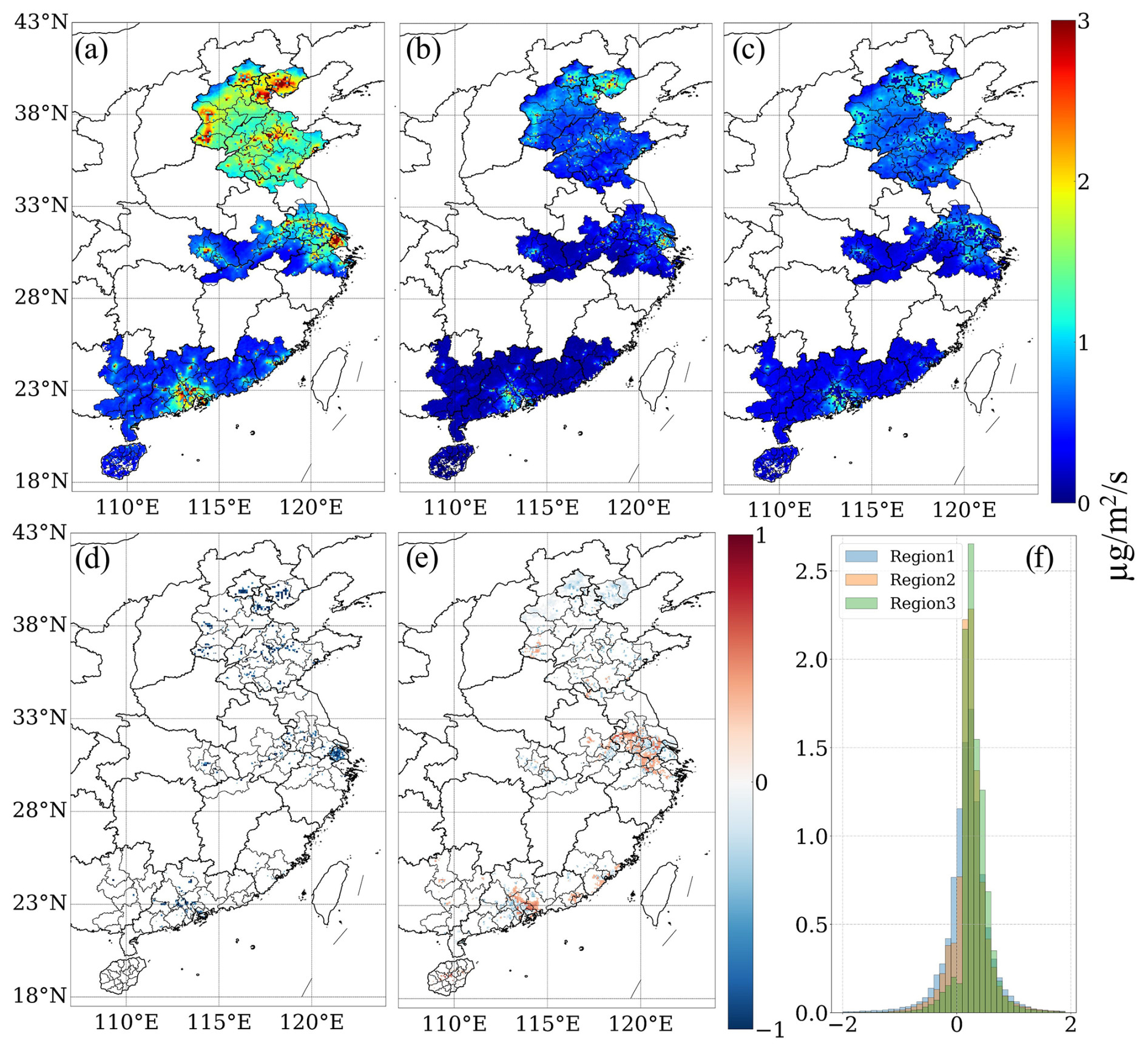
Figure 6 Representations of daily computed MCMFE-NO_x (µg m⁻² s⁻¹): (a) climatological mean of day-to-day emission, (b) climatological standard deviation of day-to-day emission, and (c) climatological mean of day-to-day uncertainty. The differences between the uncertainty and standard deviation (µg m⁻² s⁻¹) of (d) the locations where the uncertainty is smaller than the standard deviation (Diff < −0.5), (e) the locations where the uncertainty is similar to or larger than the standard deviation ($-\mathrm{0.5}<$ Diff < 0 and Diff > 0.3), and (f) the PDFs of monthly differences in the three regions.

There is minimal overlap between regions with high day-to-day variability and regions with high uncertainty. In Wuhan, for example, high variability is observed in the city center, while high uncertainty is located north of the city near the river area. Regions shown in Fig. 6e, where uncertainty is similar to (less than 0.5 µg m⁻² s⁻¹ lower) or exceeds 0.3 µg m⁻² s⁻¹ higher than day-to-day variability, are undergoing land-use changes, indicating that more robust validation and retrieval algorithms may be required in these regions. The forms of land-use and land cover changes, such as urbanization, deforestation, agricultural expansion, and infrastructure development, can significantly impact NO_x emissions through various mechanisms. These regions encompass the southern part of Hebei Province; industrializing locations in Shandong Province; suburban areas around Xuzhou, Suzhou, Wuxi, Changzhou, Zhenjiang, and Nanjing in Jiangsu Province; the northern expanded part of Wuhan; developing cities in Guangdong Province; and Xiamen. They are situated in suburban or rapidly developing rural areas that have previously been overlooked by the a priori datasets, covering 22 %, 24 %, and 12 % of regions 1, 2, and 3, respectively. In contrast, Fig. 6d illustrates that many metropolitan areas, such as centers of Beijing, Tianjin, Shanghai, Hong Kong, Guangzhou, Suzhou, Changzhou, Nanjing, Hangzhou, Wuhan, and Xuzhou, where land surfaces are not changing significantly, exhibit over 0.5 µg m⁻² s⁻¹ less uncertainty than day-to-day variability. These grids cover approximately 6 %, 5 %, and 2 % in regions 1, 2, and 3, respectively. This study highlights the importance of considering day-to-day variability in emission calculations for these areas, emphasizing the limitations of relying on monthly or annual averages from a small sample of daily data. Additionally, this research includes a comparison of the monthly mean of uncertainty and monthly variability of emission, illustrated in Fig. 6f.

3.3 Emission seesaw

The differences between MCMFE-NO_x and INTAC are outlined in Fig. 7. Analysis of the daily differences across the three regions (Fig. 7c) reveals that INTAC exceeds MCMFE-NO_x on approximately 6.9 %, 11.1 %, and 8.4 % of the grids in regions 1, 2, and 3, respectively. These grids cover small areas of the spatial domain and are in the highly developed commercial centers and sites with significant pollution, exhibiting emissions patterns consistent with enhancing energy efficiency, successful abatement or mitigation of NO_x sources, and/or potential shutdowns (Fig. 7b). However, INTAC tends to underestimate values in more grids, particularly in region 1. This includes grid areas where the day-to-day discrepancies exceed 1 µg m⁻² s⁻¹, indicating substantial sources that the a priori emissions have overlooked. The grids where the differences surpass 1 µg m⁻² s⁻¹ constitute about 55 %, 15 %, and 7 % in regions 1, 2, and 3, respectively. As evidenced in the climatological mean of the differences, a considerable quantity of emission sources has been detected in suburban regions and swiftly evolving rural areas, which are absent in the a priori datasets. The coverage of these grids in region 1 is much larger than that from the other two regions. The regions of Beijing, Tianjin, and Tangshan, as well as Jinan and Zibo in Shandong Province and Shijiazhuang, Xing Tai, and Handan in Hebei Province, have experienced substantial growth and have been extensively explored, with more active and new emission sites misidentified. In region 2, the northern part of Wuhan and the land over the Yangtze River in Jiangsu Province, especially near Suzhou and Wuxi, exhibit higher emissions than those reported in the a priori emissions. The urban core of Wuhan has remained stable over a long time due to its compact and developed nature more than 2 decades ago, but the outward expansion towards the northern sectors is new and not well constrained by the a priori data. Over the Yangtze River, some ignored emissions are not accounted for in the INTAC dataset. A portion of these emissions is attributable to development along the river, such as power plants and steel and iron factories located right next to the river. Furthermore, certain areas within region 3 contain sources that are not updated in the a priori datasets. The grids located on the southern periphery of Hong Kong are near the airport and wharf. Guangzhou has been focusing on the development of extensive scientific zones in the eastern sector and is fostering growth in Nansha in the southern sector as a new district. Along the boundary of Shenzhen, Dongguan is attracting industry from Shenzhen. This trend of new cities offering incentives is also evident in Jiangmen, with individuals migrating from Guangzhou and Foshan to Jiangmen across the border. Therefore, the higher values from MCMFE-NO_x are in line with the actual local development situation and policies, which are reasonable.

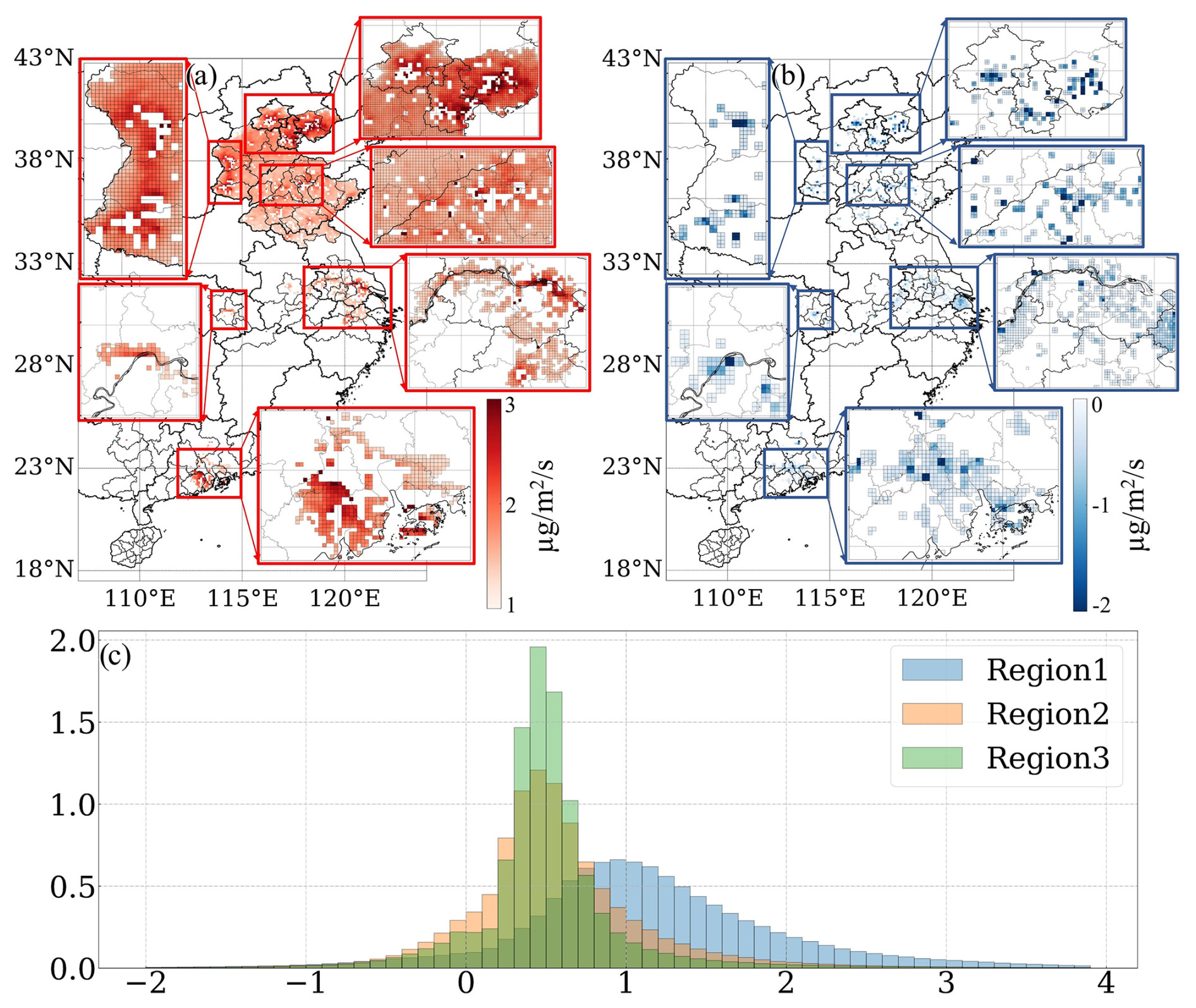
Figure 7 Map of all grids that have at least 30 d during which the difference between MCMFE-NO_x and INTAC is larger than 1.0 µg m⁻² s⁻¹ and smaller than 0 µg m⁻² s⁻¹. (a) Climatological day-by-day mean only on the days with a difference larger than the 1.0 µg m⁻² s⁻¹ cutoff. (b) Climatological day-by-day mean only on the days with a difference smaller than the 0 µg m⁻² s⁻¹ cutoff. (c) PDFs of all day-by-day and grid-by-grid differences on the grids which meet the cutoff, including the days which do not meet the cutoff over region 1 (blue), region 2 (orange), and region 3 (green).

3.4 Emissions over rivers

Emissions on and adjacent to rivers are an important research objective, as they are influenced by various aspects of anthropogenic activities and require different surface data to retrieve NO₂ column information. There have even been previous studies reporting that the water itself or shipping activity on water may be the main sources of NO_x emissions (Kong et al., 2023; Zhang et al., 2023). The study regions of this paper include the Yangtze River in Jiangsu, Anhui, and Wuhan and the Yellow River in Shandong, where the width of these rivers is close to or more than 5 km, allowing for one or more pixels of retrieved NO₂, which is mostly or solely dependent on the river environment. Moreover, there are numerous emission sources that burn coal, like power plants and steel factories, which are located right next to rivers which use the water for their cooling requirements, especially in Jiangsu (Tiwari et al., 2025). Figure 8a shows the locations of five power and industrial sources, including power plants, steel and iron factories, heat production and supply, CHP (combined heat and power), and cement factories along the Yangtze River. The total emissions in different sections are shown in Table 3. The spatial distributions of total emissions (MCMFE-NO_x and INTAC-NO_x) in the different sections of the Yangtze River are demonstrated in Fig. 8b–d. The grids which contain these sources are highlighted with red frames, and the annual total emission and uncertainty in these grids are also shown in Table 3.

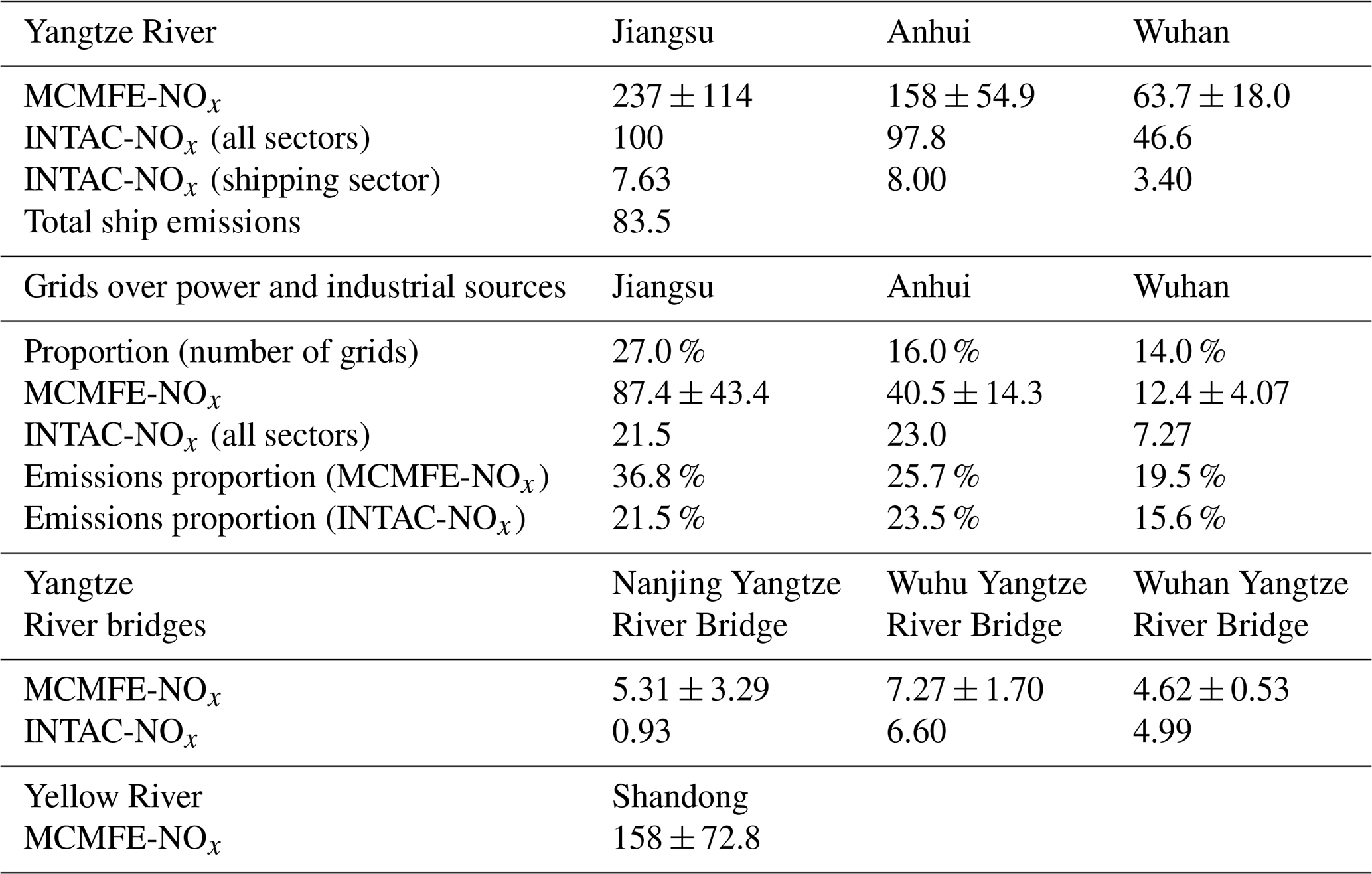
Emissions and uncertainties over the Yangtze River in Jiangsu, Anhui, and Wuhan are 237 ± 114 Kt, 157.67 ± 54.86 Kt, and 63.66 ± 18.04 Kt, respectively, for the entire year, with high values in Nanjing, Yangzhou, Ma'anshan, Wuhu, Tongling, and Wuhan. Correspondingly, emissions of INTAC are approximately 100, 98, and 47 Kt. Over the Yangtze River in Jiangsu, these highlighted grids account for 27 % of the total number but contribute nearly 37 % of the emissions. Additionally, in Anhui and Wuhan, they represent 16 % and 14 % of the total number and contribution for 26 % and 19 % of the emissions, respectively. The MCMFE-NO_x values for all grids and the proportion of MCMFE-NO_x from power and industrial sources are both higher than those in INTAC. This discrepancy indicates a potential underestimation of emissions from small and medium sources. Along the edges of the rivers, a vast amount of minor economic activities, such as utilization of machinery in agricultural practices, energy transfer devices employed in maritime activities, residential usage of controlled combustion, and small-scale industrial enterprises, is under reported. In the shipping sector of INTAC, NO_x emissions account for less than 10 % of the total emissions across all sectors, which is significantly lower than the estimates derived from the total ship emission based on an automatic identification system combined with the China Classification Society (Zhang et al., 2023). This study reports values as high as 83.5 Kt yr⁻¹, which is 10 times greater than the shipping sector estimates from INTAC. It also reveals that MCMFE-NO_x, which includes contributions from all the sectors, is unlikely to be overestimated.

In addition, the Yangtze River bridges have significant impacts on the transportation system of these regions. Figure 8 also shows the locations of the other Yangtze River bridges, which are highlighted with yellow frames. The Wuhan Yangtze River Bridge and the Nanjing Yangtze River Bridge, which were the first to be completed and opened to traffic, are also dual-purpose bridges for railways and highways. The emissions over the Wuhu Yangtze River Bridge are the highest among the bridges, and the NO_x emissions over the Nanjing Yangtze River Bridge in INTAC are considerably lower than those in MCMFE-NO_x, suggesting that heavy-transport emissions in these specific grids are also underestimated. Table 3 presents the results of three Yangtze River bridges, including the Wuhu, Wuhan, and Nanjing Yangtze River bridges.

Generally, the emissions over the Yellow River are lower than those over the Yangtze River, which aligns with expectations, as presented in Table 3. This can be attributed to the heightened caution exercised due to the river's lower water levels. Consequently, there is no coal transportation along the river. Cities situated along the Yellow River, such as Zibo, possess their own oil reserves. Chemical plants in these cities, which utilize oil as an energy source, operate at lower temperatures compared to coal-based power plants. Furthermore, it has been observed that emission values are elevated in the city center of Jinan.

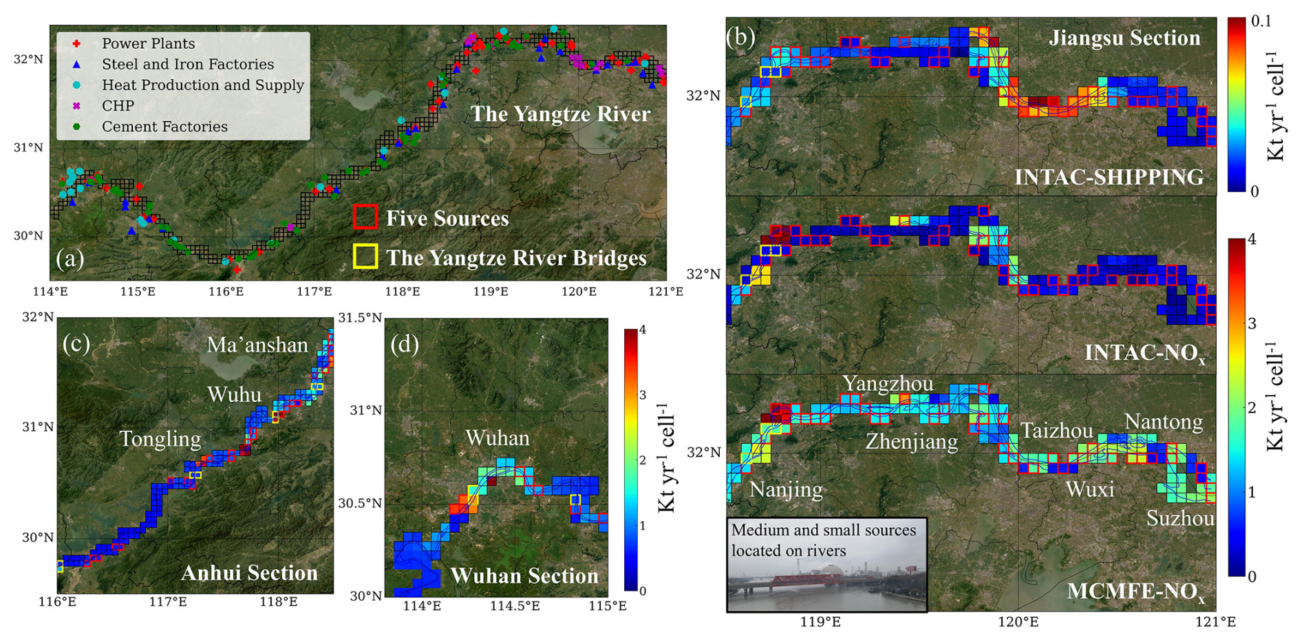
Figure 8 (a) The location of different sources along the Yangtze River. The total emissions (Kt yr⁻¹ cell⁻¹) over the Yangtze River in the different sections: (b) Jiangsu (MCMFE-NO_x, INTAC-NO_x (all sectors), and INTAC-NO_x (shipping sector)), (c) Anhui (MCMFE-NO_x), and (d) Wuhan (MCMFE-NO_x). The grid cells are defined by a latitude–longitude grid with a resolution of 0.05° × 0.05°, meaning that the area of each cell varies with latitude. This variation is accounted for in emission calculations to ensure accurate representation of emissions per unit area.

Table 3 Annual total NO_x emissions and uncertainties (Kt yr⁻¹) over the Yangtze River (MCMFE-NO_x, INTAC-NO_x, and the total ship emissions) in different sections, from different power and industrial sources (the proportion of the number and emissions), over Yangtze River bridges, and over the Yellow River.

4 Conclusions

This work applies a model-free analytical approach that assimilates daily-scale remotely sensed tropospheric columns of NO₂ from TROPOMI in a mass-conserving manner to invert daily NO_x emissions and the optimized underlying ranges of the driving chemistry, transport, and physics. The results herein are presented over three rapidly changing regions in China, each located in different climatological zones. These regions encompass densely urbanized sub-regions and surrounding rural, rapidly developing suburban, and urbanizing sub-regions. Unlike traditional approaches that mainly concentrate on the Yangtze River Delta, Beijing–Tianjin–Hebei, and the Pearl River Delta, this research adopts a more comprehensive and uniform selection based on observations and climate zones. Notably, this work includes previously large cities such as Wuhan along the middle Yangtze River; Qingdao, Jinan, and others in Shandong Province; and Hong Kong, Shantou, and Xiamen along the South China Sea.

One important conclusion relates to the parameter α₁, observed in the three research areas, which peaks in July or August and reaches a minimum in December and January due to UV radiation. Furthermore, α₁ shows a second peak in February, reflecting varied economic and energy demands during the Chinese New Year period. Among the cities in the research areas, the highest values are found in Heze, Lianyungang, and Beihai, all of which have a large number of industries. Source attribution is also quantified with respect to the local thermodynamics of the combustion temperature, revealing distinct characteristics of α₁ across five industrial sources. The 50th percentile range and the hl_ratio allow for clear differentiation and unique attribution of the five source types. Note that the α₁ values used herein are found to match well with observations in urban areas (Karl et al., 2023) and areas with large industrial sources (Li et al., 2023a; Lu et al., 2015), although they are far outside of the bounds currently used by most models, indicating that the current generation of atmospheric models may not be able to capture such observed emissions sources well (Beirle et al., 2019).

Several additional scientific points of interest are revealed regarding the MCMFE-NO_x results. First, the day-to-day and grid-by-grid emissions and uncertainties are found to be 1.96 ± 0.27 µg m⁻² s⁻¹ on pixels with available a priori values (1.94 µg m⁻² s⁻¹), while 1.22 ± 0.63 µg m⁻² s⁻¹ extra emissions are found on pixels in which INTAC is lower than 0.3 µg m⁻² s⁻¹. Some grids show lower MCMFE-NO_x compared to INTAC, mainly in urbanized and polluted areas, possibly due to energy efficiency, abatement efforts or mitigation of NO_x sources, and/or potential shutdowns. The illustration also highlights the grid areas where the daily differences exceed 1 µg m⁻² s⁻¹, indicating significant sources missed by the a priori datasets.

Second, rivers are a crucial research focus because they impact numerous aspects of human activities. Emissions of industrial sources from missing sites adjacent to the Yangtze River are found to be 161. ± 68.9 Kt yr⁻¹, which is 163 % higher than the a priori. There are numerous emission sources that burn coal, like power plants and steel factories, which are located right next to the river to use water for their cooling requirements, especially in Jiangsu Province. Over the Yangtze River in Jiangsu Province, these highlighted grids account for 27 % of the total number but contribute nearly 40 % of emissions. Moreover, in Anhui Province and Wuhan, they represent 16 % and 14 % of the total number, with a contribution of 26 % and 19 % of emissions, respectively. These findings indicate that the contributions from small-scale industries in pixels on or adjacent to rivers offer a significant source of unaccounted for NO_x emissions, which is shown to be larger than the amounts reported from biological sources in lakes (Kong et al., 2023) and from inland shipping activities (Zhang et al., 2023).

Third, there is little overlap between high day-to-day variability and high uncertainty. The uncertainty over land surfaces which are not changing is smaller than the day-to-day variability, emphasizing the importance of considering day-to-day variability in emissions. Conversely, uncertainty over areas experiencing land-use changes or over water is similar to or larger than the day-to-day variability, indicating that more robust validation and retrieval algorithms may be required in these regions.