German methane fluxes estimated top-down using ICON–ART – Part 1: Ensemble-enhanced scaling inversion

This two-part study explores the quantification of greenhouse gas emissions using atmospheric observations in order to validate national emission inventories. Inverse methods can support emission quantification at the national scale based on observations and atmospheric transport simulations, yet, they are often limited by the observation coverage, transport model uncertainties, and inversion methodologies. Here, we introduce a system for regional estimation of methane fluxes and apply this to Central Europe with a focus on Germany, where we distinguish emissions from different anthropogenic sectors. We evaluate the robustness of the method using sensitivity tests with in-situ observations from the Integrated Carbon Observation System (ICOS). Using synthetic observation experiments, we estimate the impact of transport errors on the flux estimates. The atmospheric transport is calculated employing the numerical weather prediction model ICON with its module ART at 6.5 km resolution, sampling the meteorological uncertainty with a 12-member transport ensemble. The same transport ensemble is used to generate pseudo-observations with a simulated transport uncertainty. Posterior fluxes are estimated with a synthesis inversion method for three different approximations of the model–observation error covariance matrix. We find that using ensemble-estimated transport uncertainties can significantly reduce the random error of emission estimates. Our results highlight the importance of analyzing biases in flux inversions for reliable, observation-based emission estimates.

1 Introduction

Quantifying greenhouse gas (GHG) emissions is essential for effective mitigation of anthropogenic climate change. Atmospheric GHG inversions provide such quantification by connecting the observed atmospheric composition to surface fluxes using transport models. This so-called “top-down” approach is complementary to “bottom-up” emission estimates, which are based on activity data and emission factors (IPCC et al., 2019). Top-down emission estimates can be used to validate national bottom-up GHG inventories reported to the United Nations Framework Convention on Climate Change (UNFCCC) (Manning et al., 2003, 2011; Henne et al., 2016). Such national-scale estimates are typically limited by the observation coverage (Petrescu et al., 2023) and uncertainties in atmospheric transport modeling (Gerbig et al., 2008). This motivates estimating methane emissions in the comparably well-observed Central Europe using a high-resolution transport model and applying methods from numerical weather prediction (NWP) to estimate the transport uncertainty.

Regional top-down estimates of long-lived GHG can be based on different types of transport models. Lagrangian models calculate trajectories from selected locations by moving with air parcels transported by the wind. They have been widely used for inversions of trace gases like halocarbons, nitrous oxide and methane (CH₄) in European regions, see e.g., Stohl et al. (2009), Ganesan et al. (2015), Henne et al. (2016). In contrast, Eulerian models – such as ICON–ART – continuously transport trace gas concentrations through three-dimensional grid boxes. Although they are computationally more expensive for cases where a relatively small number of trajectories would suffice, they become superior when the amount of data grows and, as Engelen et al. (2002) pointed out, open the road for data assimilation methods as used in NWP. Among the Eulerian models, also NWP models have been used for regional flux inversions of CO₂ (Lauvaux et al., 2013) and CH₄ (Steiner et al., 2024b). Regardless whether Lagrangian or Eulerian or even combined approaches (Rigby et al., 2011) are applied, the top-down estimation requires solving an inverse problem (Enting, 2002). Eulerian transport model based inversions may employ emission ensembles, as in Steiner et al. (2024b) with a localized Kalman filter, and other data assimilation methods (see, e.g., Meirink et al., 2008). Alternatively, the method of synthesis inversion scales a set of a priori emission categories (Kaminski et al., 2001).

In this work, we introduce a system for national-scale top-down estimation of CH₄ emissions based on modeling experience from NWP. We analyze the benefit of constraining the transport uncertainty using a meteorological ensemble as proposed by Ghosh et al. (2021) and Steiner et al. (2024a). A synthesis inversion method is used to estimate emissions with a focus on Germany based on high-resolution a priori emissions from national reporting and in situ observations of atmospheric CH₄ concentrations.

In the present Part 1 of this two-part study, we describe our new inversion system and evaluate its performance. Section 2 introduces the method with a detailed description of the uncertainty estimation. The description of the inversion system is completed by the input data described in Sect. 3. In Sect. 4, we analyze the performance using synthetic observation experiments and test the sensitivity to tuning parameters with real observations. We conclude in Sect. 5 and refer to Part 2 (Bruch et al., 2025a) for a discussion of the emission estimates obtained using real observations.

2 Method

We use a synthesis inversion method (Kaminski et al., 2001) that scales the CH₄ fluxes to optimize the agreement of model predictions and observations. In this method, the fluxes are initially grouped into a manageable set of flux categories. Here, these are 46 categories that subdivide the fluxes by region and emission sector. With the Eulerian transport model, the concentration from each flux category is calculated separately at all grid cells and time points. At the location and time of the observations, the model writes out the predicted concentrations from the flux category contributions and their sum is compared to the observed concentration. The inversion then minimizes the mismatch between model prediction and observations by scaling each of the flux categories by one number – the scaling factor – making use of the linear relation between fluxes and concentrations in the atmosphere. Thus, the inversion result consists of one scaling factor for each flux category. By multiplying the a priori fluxes with the scaling factors we obtain the a posteriori fluxes. This scaling method cannot provide a correction where a priori fluxes are zero (Kountouris et al., 2018). However, this is less of a problem for CH₄, as inventories can collect where methane-emitting activities are normally located, but emission factors which translate the activities into bottom-up emissions are uncertain (Dammers et al., 2024).

The described method relies on high quality model predictions as well as accurate concentration observations. To match these requirements, we have carefully chosen the configuration of the transport model (Sect. 2.1) and consider the specific difficulties in modeling strong plumes (Sect. 2.2). Selected observational data are employed to remedy model boundary effects and therefore improve the overall model predictions (Sect. 2.3). In Sect. 2.4, we introduce the Bayesian inversion framework. To assess whether deviations between model and observations contain information on the fluxes, we estimate the model uncertainty and error correlations. We compare three different methods for estimating these uncertainties and correlations (Sects. 2.5 and 2.6). Furthermore, we define the time window and a priori uncertainties of the inversion (Sect. 2.7 and 2.8). A summary of the method and data streams will be provided in Sect. 3.5.

2.1 Transport simulation

2.1.1 Transport model

The atmospheric transport is simulated using the NWP model ICON (Zängl et al., 2015) in a configuration close to operational NWP at Germany's Meteorological Service (DWD), extended with the module for Aerosol and Reactive Trace gases (ART) (Rieger et al., 2015; Schröter et al., 2018). The model is run in limited area mode for a domain covering large parts of the European continent (latitudes 34 to 70° N, longitudes 21° W to 59° E, see Fig. 1) with a horizontal resolution of 6.5 km (ICON grid R3B8) and 74 vertical levels up to a maximal height of 22.77 km. The ICON model simulates the meteorology and the tracer transport. Re-initialization of the meteorological fields every 24 h with operationally produced analysis fields ensures that the meteorology stays close to reality. The surface CH₄ fluxes are provided to the transport model using the online emission module (Jähn et al., 2020; Steiner et al., 2024b). We do not simulate any chemical reactions, because the typical lifetime of CH₄ in the atmosphere is much longer than the time that an air parcel typically spends in our modeling domain.

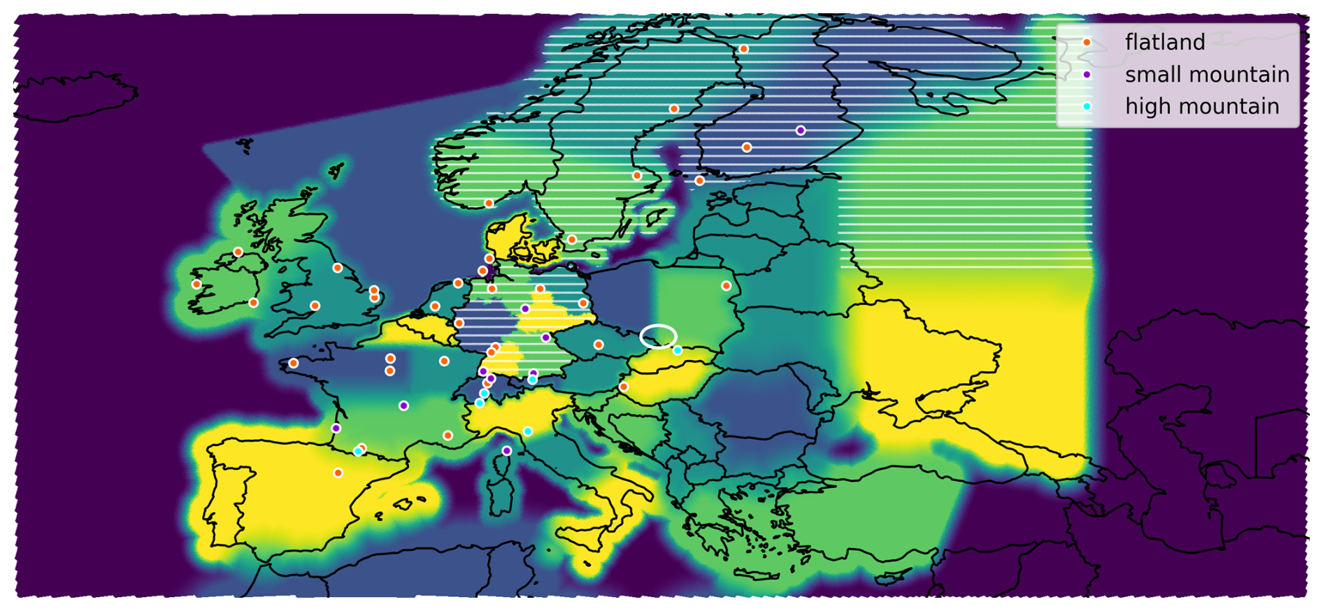
Figure 1 Model domain, colored to distinguish 35 patches defining regional flux categories. Observation sites (dots) are colored by the choice of model equivalent height (see Table C1). Dark blue at the domain boundary indicates regions for which emissions are not categorized and therefore not modified in the inversion. Other colors only distinguish neighboring patches. In white hatched regions, natural fluxes are also categorized and scaled. A white ellipse marks the Upper Silesian Coal Basin, in which fugitive emissions define their own flux category. In Germany, the map shows the six regions used for the agricultural sector. For other sectors in Germany, we use four regions: south (yellow and light green), west (dark blue), north (light green), and east (dark green and yellow).

For long living tracers like methane, the correct treatment of the lateral boundary concentrations is of importance. Therefore, we extended the model by implementing lateral boundary nudging for ART tracers in order to obtain smooth fields and avoid strong spatial gradients. The nudging is limited to a boundary zone of width <250 km. Further, so-called meteogram output has been implemented for ART tracers, providing model output in the vicinity of observation locations with high temporal resolution.

2.1.2 Meteorological ensemble

For improved uncertainty estimates, we run a meteorological ensemble of 12 members. Each ensemble member uses different meteorological initial and lateral boundary conditions from the operational ensemble data assimilation used for global NWP at DWD (Schraff et al., 2016; Reinert et al., 2025). Since our meteorological input fields and the transport model setup are taken from operational NWP at DWD, the ensemble provides a reasonable estimate for the meteorological uncertainty in our model, including uncertainties in the simulated wind field and atmospheric stability.

In the following, we distinguish a so-called deterministic model run providing the best estimate of the modeled CH₄ concentration, and the ensemble runs providing 12 different CH₄ concentrations to estimate the uncertainty. The ensemble will only be used to estimate model uncertainties and error covariances (see Sect. 2.5), and to generate pseudo-observations (Sect. 3.4).

2.1.3 Definition of flux categories

Estimating CH₄ fluxes in >10⁵ grid cells based on 50 observation sites seems impossible without reducing the number of degrees of freedom of the fluxes. Here, we reduce the degrees of freedom drastically by parametrizing the fluxes using only 46 basis vectors. A basis vector in this parametrization is a flux category that contains all fluxes from one region, possibly limited to specific emission sectors. For example, we define all anthropogenic emissions from Denmark as one flux category. We thereby assume that the distribution of anthropogenic emissions within Denmark is correct in the a priori and only allow the inversion to adjust the total emissions from Denmark.

We define the flux categories with the primary aim of providing an accurate estimate of emissions from Germany, resolving federated states where possible, to address the requirements of potential stakeholders. When distinguishing emission sectors, we stay close to the national reporting by using definitions from the gridded aggregated nomenclature for reporting (GNFR, Veldeman et al., 2013). For the agricultural sector (GNFR sectors K+L), which contributes roughly two thirds of all German CH₄ emissions, we distinguish six regions within Germany as depicted in Fig. 1. For the sum of all other sectors – excluding natural and LULUCF fluxes – we distinguish four regions, i.e., the federated states south: Baden-Wuerttemberg and Bavaria, west: North Rhine-Westphalia, Hesse, Rhineland-Palatinate and Saarland, north: Lower Saxony, Bremen, Hamburg and Schleswig-Holstein, as well as east: Mecklenburg-Western Pomerania, Brandenburg, Berlin, Saxony, Saxony-Anhalt and Thuringia. Natural plus LULUCF fluxes in Germany are treated as a single flux category.

Outside Germany, we do not distinguish sectoral emissions, with one exception. Agriculture emissions in the Netherlands form their own category, as we found that they strongly influence the CH₄ concentrations in Germany, caused by the proximity and high emission rates in the Netherlands. We define further categories by area for anthropogenic emissions excluding LULUCF such that a comparably high resolution is obtained in regions near Germany with high observation coverage. These area-defined flux categories follow borders as feasible for the inversion. Areas with small expected influence on inversion results for Germany are combined in large categories, such as Spain plus Portugal, Türkiye plus Greece, and large areas east of Poland. All area-defined categories are shown in Fig. 1 and an overview of the sector resolution is given in Table 1.

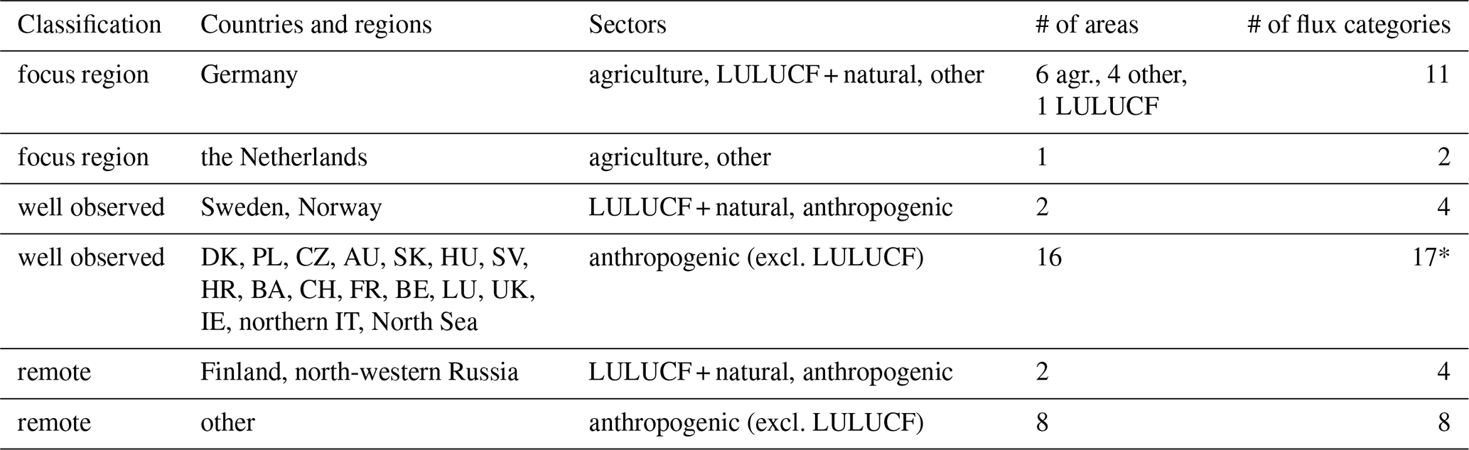
Table 1 Overview of sectors distinguished in the inversion and number of flux categories. We distinguish the focus region, well-observed regions near the focus region, and regions in large distance from the focus region (“remote”). The latter are split in very large flux categories with low a priori uncertainty. Natural plus LULUCF fluxes are separated from other anthropogenic emissions only in regions where the natural fluxes are strong and in Germany. One extra category in the well-observed regions is the Upper Silesian Coal Basin (marked * in the last column). See Fig. 1 for the definition of flux categories on the map.

We treat natural plus LULUCF fluxes separately and categorize them only in Germany, Scandinavia, and the north-eastern part of our domain (hatched regions in Fig. 1). This is motivated by strong CH₄ emissions from wetlands in summer in Scandinavia and northern Russia in our prior (Segers and Houweling, 2020). Uncategorized fluxes – whether natural or anthropogenic – are not scaled in the inversion, but still included in the transport simulation such that no fluxes are discarded. To avoid strong spatial gradients in the concentration fields, the boundaries between different area-defined categories are smoothened as visualized in Fig. 1.

We furthermore define a separate flux category for the strongest CH₄ plume in Central Europe to mitigate the plume localization problem described below (Sect. 2.2). These are fugitive emissions from the Upper Silesian Coal Basin with yearly emissions of 567 kt in our prior (white ellipse in Fig. 1).

2.1.4 Tracer assignment in the transport model

In the transport simulation, we consider not only the categorized fluxes, but also the CH₄ from lateral boundaries and from uncategorized emissions. Overall, we simulate the transport of 50 tracer fields in the deterministic model run:¹

• (i)

  Sum of all anthropogenic emissions excluding LULUCF. This constitutes a single, common tracer.

• (ii)

  Sum of all natural plus LULUCF fluxes. This constitutes another single, common tracer, which summed with (i) covers all a priori emissions in the domain.

• (iii)

  Far field. The far field contains the CH₄ from initial and lateral boundary conditions.

The sum of (i)–(iii) is the total a priori CH₄ concentration. The a posteriori concentration is not computed directly. Instead, we treat the deviation of the posterior concentration from the prior as a perturbation. To compute this perturbation, we simulate the transport of each flux category:

• (iv)

  Flux categories. For each of the 46 flux categories an own tracer field is defined. To avoid the accumulation of categorized CH₄ beyond the time scale on which we consider the modeled transport reliable, we set an artificial decay rate of these concentrations. After emission, the concentration in these tracer fields decays exponentially with a mean lifetime of 5 d. This technical feature constitutes a localization in time similar to the commonly used localization in space (e.g., Steiner et al., 2024b) and allows a waning of sectoral and regional attribution over a few days. This regulates that any attribution of a CH₄ anomaly to a certain region or sector is only attempted if the emission was fresh or a few days ago. Furthermore, this allows us to save computing time by limiting the transport of these flux category tracer fields to altitudes below 8 km. The artificial decay rate affects the posterior concentration and the sensitivity of the inversion to changes in the emissions. However, assuming that the typical time between emission and observation is short compared to the artificial lifetime and in the presence of transport model errors, we expect that this feature of our inversion system leads to more robust results.

• (v)

  Auxiliary field for plume detection. For the purpose of investigating the model uncertainty due to the plume from the Upper Silesian Coal Basin, an auxiliary tracer is added (see Sect. 2.6.1). This tracer is never added to the total CH₄ concentration but only serves as an indicator for the plume location.

2.2 Plume localization problem

In our transport simulation and inversion, we address the specific challenge posed by plumes from high emissions in small areas. The inversion may be biased for such plumes due to the so-called double penalty issue (Vanderbecken et al., 2023). In cases where our model falsely predicts that the plume reaches an observation site, the inversion will reduce the emissions to improve the agreement with the observation. In the opposite case, when the model fails to predict that a plume reaches the observation, the inversion will not change the plume emission amount but will wrongly increase emissions in other areas instead. This can cause a systematic underestimation of fluxes from localized plumes. To avoid biases in the inversion results, we suggest to treat strong plumes separately, with their own flux categories. This allows us to quantify the problem (see Sect. 4.2) and to limit the plume penalty influence on other flux categories.

2.3 Far-field correction

For cases where the model predicts almost no influence from our categorized emissions (i.e., clean air cases), deviations between model and observations point to the need for correcting the CH₄ advected across the lateral boundaries – here referred to as “far field”.² For our regional inversion problem, it is essential to separate the CH₄ emitted within the domain from the far field, in order to avoid model biases which would confound the aspired flux scaling (see, e.g., Chen et al., 2019, for CO₂). To minimize potential biases arising from imperfect boundary conditions, we construct a correction field which is added to the modeled far-field concentration in the whole domain after the transport simulation. We require this correction field to be smooth on spatial and temporal scales 320 km (horizontal), 1 km (vertical), and 16 h (time). We construct this far-field correction using a Kalman smoother as described in detail in Appendix A. This construction uses only clean-air observations with a cumulated signal of all flux categories of ≤20 ppb and a total signal from emissions within our domain of ≤50 ppb.

Figure 2 shows a statistical overview of the far-field correction when using real observations (red line) or pseudo-observations (shaded area). The considered pseudo-observations are generated from the ensemble members of the transport simulation and represent the case where simulated emissions and boundary conditions are perfect, i.e., equal to the truth. The far-field correction range is usually limited to ±10 ppb when using real observation data and ±5 ppb in the synthetic observation experiments (Fig. 2a) with variations of a few ppb per day (Fig. 2b). The broad distribution of the root mean square (RMS) for different observation sites and months in Fig. 2c indicates significant differences among the stations when using real observations.

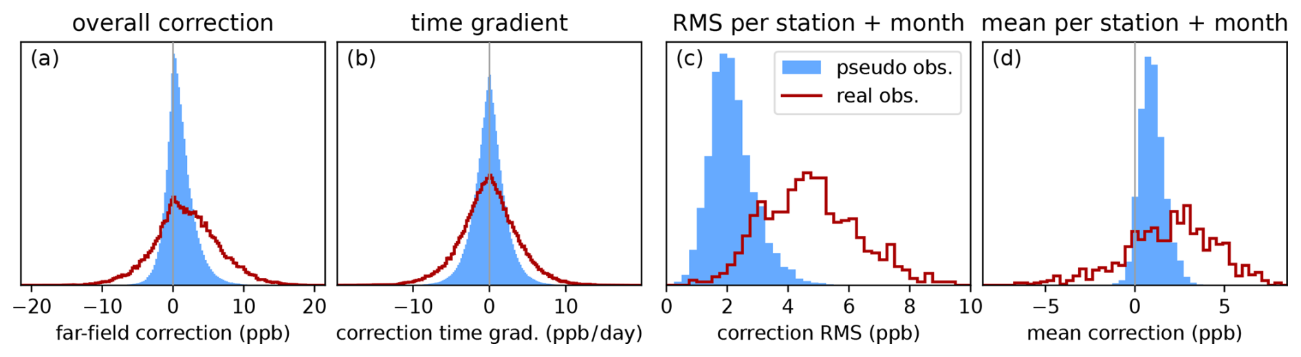
Figure 2 Statistical evaluation of the far-field correction at the observation coordinates when using synthetic observations (light blue area) or real observations (dark red line). Considering all data points used in the inversion, histograms of the far-field correction show (a) the range of the correction and (b) its temporal variation. For each station, month, and realization of pseudo-observations, we compute the root mean square (RMS) and the mean (or bias). Histograms combining these values for all stations and months are shown in (c) and (d).

Figure 2d shows that the correction has a small bias towards positive corrections even when using synthetic observations with unbiased fluxes and boundary conditions. This is partially due to the pseudo-observations, which are biased by +0.5 ppb compared to the simulated concentrations due to details of the transport model configuration. The other part of the bias hints to a more general problem. We construct the far-field correction using observations for which the model predicts clean air, i.e., a low signal from the emissions. Since the transport model is not perfect, this introduces a sampling bias: We select more observations for which the model underestimates the concentrations and thereby increase the bias to 1.2 ppb. In response to this bias, the far-field correction increases the simulated concentrations by 1.0 ppb.

The sampling bias will likely also occur when working with real observations. But the estimated correction bias of 0.6 ppb due to the sampling is small compared to the accuracy of the Copernicus Atmosphere Monitoring Service (CAMS) inversion-optimized data product used for our boundary conditions (Segers et al., 2023) (see Sect. 3.1). We therefore do not expect a significant impact on the emission estimates.

2.4 General approach of the inversion framework

We use a Bayesian inversion to optimize the agreement of model and observations. We define a vector of scaling factors – in our application s∈ℝ⁴⁶ – consisting of one prefactor for each flux category. This low-dimensional parametrization of the fluxes leads to the optimization problem

$$\begin{array}{}\text{(1)}& \begin{array}{rl}{\mathit{s}}^{\text{post}}=\underset{\mathit{s}}{\text{arg\hspace{0.17em}min}}\mathit{\{}& \frac{\mathrm{1}}{\mathrm{2}}(\mathit{y}-\mathbf{H}\mathit{s}-{\mathit{x}}^{\text{ff}}{)}^{\top }{\mathbf{R}}^{-\mathrm{1}}(\mathit{y}-\mathbf{H}\mathit{s}-{\mathit{x}}^{\text{ff}})\\ & +\frac{\mathrm{1}}{\mathrm{2}}(\mathit{s}-{\mathit{s}}^{\text{prior}}{)}^{\top }{\mathbf{B}}^{-\mathrm{1}}(\mathit{s}-{\mathit{s}}^{\text{prior}}\left)\mathit{\right\}}\end{array}\end{array}$$

for the posterior scaling factors s^post. Here, the first term penalizes the deviation from the observed concentrations, and the second term penalizes the deviation from the prior fluxes. In the first term, the vector y of observed concentrations is compared to the model prediction, which consists of the contribution Hs of fluxes within the model domain and the modeled far field x^ff including the far-field correction. All model predictions (x^ff and Hs) are already projected to the observation space. The contribution of fluxes Hs depends linearly on the vector s. The difference between modeled and observed values is weighted by the error covariance matrix R describing the combined uncertainty of the transport model and the observations. With the second term we constrain the deviation of s from a priori scaling factors s^prior (${\mathit{s}}_k^{\text{prior}}=\mathrm{1}$ for all k) with an error covariance matrix B characterizing the a priori uncertainty (see Sect. 2.8).

In Eq. (1), the model observation operator H connects the space of scaling factors (vectors s^prior, s^post) to the observation space (vectors y, x^ff). Computing H requires the transport model which distinguishes the flux categories. The setup is designed for optimizing a low-dimensional vector s^post of scaling factors (∼10² degrees of freedom) using a large number of observations (∼10⁴), but an extension to more degrees of freedom and/or more observations is possible.

2.5 Approximations for the error covariance matrix R^′

The definition of the error covariance matrix R in Eq. (1) is crucial for the inversion. R describes the combined uncertainties and correlations of observations and model predictions. In our case, the observation uncertainty (usually ≲1 ppb, ICOS RI, 2020) is small compared to the ensemble-estimated transport uncertainty (typically 5 to 10 ppb). We therefore focus on the model uncertainty.

Many works have used diagonal R matrices (e.g. Bergamaschi et al., 2010; Petrescu et al., 2023; Steiner et al., 2024b) and others found non-diagonal approximations for R (Ghosh et al., 2021; Steiner et al., 2024a). Here, we use the diagonal R for comparison to two different ways of constructing a non-diagonal R matrix from our transport ensemble. We therefore compare three ways of constructing R:

Diagonal R:

This baseline scenario considers a diagonal R matrix and discards all information from the transport ensemble.

Prior R:

In a standard ensemble approach, we construct R using the transport ensemble with a priori fluxes.

Posterior R:

We extend the standard approach by estimating R using the posterior fluxes in the transport ensemble.

The construction of the different R matrices consists of two steps that are described below. First, we construct a matrix R^′ that estimates the dominant uncertainties and correlations using one of the three methods. Second, we obtain R from R^′ by inflating and adding additional uncertainties to mitigating some known issues of the inversion (Sect. 2.6).

2.5.1 Diagonal R

In the baseline scenario of a diagonal R matrix, all observation and model uncertainties are assumed to be uncorrelated. However, it is known that model predictions for observations separated by only 1 h usually have correlated errors. To avoid underestimating the overall uncertainty without introducing correlations in R, we assume high uncertainties of each observation. Following Steiner et al. (2024b), we assume that the signal from CH₄ emissions within our domain will generally increase the model uncertainty in the predicted CH₄ concentration. This motivates defining ${\mathbf{R}}_{ii}^{\prime }={\mathit{\sigma }}_{\text{const}}^{\mathrm{2}}+(\mathit{\beta }\mathbf{H}{\mathit{s}}^{\text{prior}}{)}_i^{\mathrm{2}}$ where σ_const=10 ppb and β=0.5 are scalar tuning factors. Index i labels observation data points that are typically distinguished by location, time, and sampling height. The diagonal R scenario uses crude approximations because the selection of observations is designed for an inversion that can handle correlations. However, we will obtain qualitative insights from the comparison to the other approximations for R.

2.5.2 Prior R

This approximation of R is based on an ensemble of M=12 different transport realizations. The potential of using a small transport ensemble for estimating model uncertainties was demonstrated by Steiner et al. (2024a). We can use the covariance of the ensemble members to estimate the transport uncertainty. We define

$$\begin{array}{}\text{(2)}& {\mathbf{R}}_{ij}^{\prime }={\mathbf{C}}_{ij}{\displaystyle \frac{\mathrm{1}}{M-\mathrm{1}}}\sum _{m=\mathrm{1}}^M({\mathit{x}}_i^m-{\stackrel{\mathrm{‾}}{\mathit{x}}}_i)({\mathit{x}}_j^m-{\stackrel{\mathrm{‾}}{\mathit{x}}}_j)+{\mathit{\delta }}_{ij}{\mathit{\sigma }}_{\text{const}}^{\mathrm{2}},\end{array}$$

where ${\mathit{x}}_i^m$ is the prediction of ensemble member m for observation y_i assuming a priori fluxes, ${\stackrel{\mathrm{‾}}{\mathit{x}}}_i=\frac{\mathrm{1}}{M}{\sum }_m{\mathit{x}}_i^m$ is the ensemble mean, and σ_const=10 ppb is a constant uncertainty added to each observation. With this uncorrelated uncertainty σ_const, we account for additional uncertainties, such as representativity errors inherent to a simulation at finite resolution. Indices i,j label observation data points. By C_ij we denote a localization in space and time such that C_ii=1 and C_ij=0 for any observations i and j that we expect to be uncorrelated because of their temporal or spatial separation. In the application to Germany, we choose C_ij to be a Gaussian localization matrix with standard deviations 6 h (time), 319 km (horizontal), and 400 m (vertical). We use the notation δ_ij=1 if i=j and δ_ij=0 if i≠j.

2.5.3 Posterior R

The posterior R approximation is a variation of the prior R approximation. In Eq. (2), we use model predictions for the concentrations ${\mathit{x}}_i^m$. Instead of using the prior concentrations as in the prior R construction, we can define ${\mathit{x}}_i^m$ as the posterior concentrations and thereby allow ${\mathit{x}}_i^m$ to change as the inversion changes the fluxes. This leads to a self-consistent estimate of R^′ in the inversion. Consequently, Eq. (2) remains valid but ${\mathit{x}}_i^m$, R^′, and R become functions of the scaling factors s. Since R is estimated using posterior scaling factors, we call this method the posterior R inversion as opposed to the prior R estimate. To compute the posterior concentration ${\mathit{x}}_i^m\left(\mathit{s}\right)$ for each ensemble member without prohibitive computational effort, we use an approximation described in Appendix B.

As opposed to the diagonal R and prior R inversion with fixed R, the posterior R inversion does not allow for a closed form solution of Eq. (1). To solve the minimization problem in Eq. (1) numerically, we used SciPy's “trust-exact” implementation of a trust-region method (Virtanen et al., 2020; Moré and Sorensen, 1983; Conn et al., 2000). Within each iteration, the incomplete LU decomposition (Li et al., 1999; Li and Shao, 2011) of the sparse matrix R(s) is the most computationally expensive task when the number of observations is large.

2.6 Additional uncertainties and final error covariance matrix R

The previously derived approximations for the error covariance matrices R^′ describe our knowledge of the transport uncertainty and the observation uncertainty. In the next four steps, we increase uncertainties and include other possible sources of uncertainty to obtain approximations for R that are suitable for the inversion.

2.6.1 Mitigating the plume localization problem

To reduce the bias which we predicted for strong plumes in Sect. 2.2, we increase the uncertainty for all observations that are likely affected by a plume. The transport ensemble will already lead to an increased uncertainty when the model cannot predict reliably whether a plume hits an observation site. But with an ensemble of only 12 members, this will not cover all cases where model and observations deviate. We therefore introduce an auxiliary tracer that contains emissions from the Upper Silesian Coal Basin, spatially smoothened on a length scale of 0.4° (one standard deviation of a Gaussian filter). Denoting the concentration of this tracer at observation i by ρ_i, we increase the uncertainties to ${\mathbf{R}}^{\text{step\hspace{0.17em}1}}={\mathbf{R}}_{ij}^{\prime }+\mathrm{0.25}{\mathit{\rho }}_i^{\mathrm{2}}{\mathit{\delta }}_{ij}$.

2.6.2 Dynamic uncertainty inflation

To avoid potential biases through site-specific small-scale features not captured in the model, we aim to base our inversion on many observations. To this end, we limit the influence of individual data points on the inversion result by inflating the uncertainty further in the case of a very large disagreement between model and observation. This is achieved by an uncertainty inflation of individual observations until the deviation $\mathit{\mu }=\mathit{y}-\mathbf{H}{\mathit{s}}^{\text{prior}}-{\mathit{x}}^{\text{ff}}$ between model and observations is at most three standard deviations of the resulting error covariance matrix ${\mathbf{R}}_{ij}^{\text{step\hspace{0.17em}2}}=g_i{g}_j{\mathbf{R}}_{ij}^{\text{step\hspace{0.17em}1}}$, i.e., $g_i=max\mathit{\{}\mathrm{1},\frac{\left|{\mathit{\mu }}_i\right|}{\mathrm{3}\sqrt{{\mathbf{R}}_{ii}^{\text{step\hspace{0.17em}1}}}}\mathit{\}}$. This is justified because large deviations between model and observations, $\left|{\mathit{\mu }}_i\right|>\mathrm{3}\sqrt{{\mathbf{R}}_{ii}^{\text{step\hspace{0.17em}1}}}$, are likely caused by local pollution or modeling problems that are not captured appropriately in our uncertainty estimate. This correction makes sure that inversion results will be based on many observations and no single measurement can have an extreme impact. At the same time, this method it is less sensitive to tuning parameters than discarding outliers completely.

2.6.3 Static uncertainty inflation

The transport ensemble in the prior R and posterior R construction may not necessarily include the full uncertainty of the transport model, and the localization C_ij further reduces the simulated uncertainty by suppressing correlations. This motivates another inflation of the uncertainty to avoid overconfidence in the model prediction. We inflate the uncertainty by a factor f_i>1 depending on the observation site of observation i, leading to ${\mathbf{R}}_{ij}^{\text{step\hspace{0.17em}3}}=f_i{f}_j{\mathbf{R}}_{ij}^{\text{step\hspace{0.17em}2}}$. We choose f_i=2 except for some stations with known difficulties, for which f_i=3 (see Table C1). To keep the methods for constructing R comparable, we apply this inflation also to the diagonal R matrix.

2.6.4 Far-field uncertainty

We furthermore account for the uncertainty in the far-field correction, although the effect of this additional uncertainty is small. We define ${\mathbf{R}}_{ij}={\mathbf{R}}_{ij}^{\text{step\hspace{0.17em}4}}={\mathbf{R}}_{ij}^{\text{step\hspace{0.17em}3}}+\mathrm{0.5}\left|{\mathit{c}}_i{\mathit{c}}_j\right|{\stackrel{\mathrm{̃}}{\mathbf{C}}}_{ij}$ where c_i denotes the smooth correction field introduced in Sect. 2.3 at observation i and ${\stackrel{\mathrm{̃}}{\mathbf{C}}}_{ij}$ is the Gaussian localization matrix constructed by the length and time scales of the far-field correction (see Appendix A).

2.6.5 χ² analysis

To assess whether the estimated uncertainties are reasonable, one can compute the ${\mathit{\chi }}^{\mathrm{2}}/N_{\text{dof}}$ value (Pearson, 1900). This value compares the a priori model–observation mismatch to the uncertainty assumed for this mismatch (see Appendix D for details). A value of ${\mathit{\chi }}^{\mathrm{2}}/N_{\text{dof}}>\mathrm{1}$ indicates that uncertainties are underestimated, whereas values smaller than one indicate the opposite. When comparing the observations to the far-field-corrected model, we find ${\mathit{\chi }}^{\mathrm{2}}/N_{\text{dof}}\approx \mathrm{0.16}$ for the prior R inversion when using real observations (see Table 2). In an idealized setup, this indicates that the uncertainties of the model-data mismatch are overestimated by a factor 2.5. This implies that our uncertainty inflation by a factor f_i=2 for most observations seems unnecessary in the idealized setup. However, our data can contain unknown biases in transport and boundary conditions, and simplifying assumptions about the representativity of the low-dimensional state space of the inversion. We contain these potential issues of unknown error components by inflating the uncertainties.

Table 2 Median of ${\mathit{\chi }}^{\mathrm{2}}/N_{\text{dof}}$ for different configurations. ${\mathit{\chi }}^{\mathrm{2}}/N_{\text{dof}}$ for the prior R inversion also serves as an approximation for the posterior R inversion. Synthetic observations are generated using the ensemble simulation, assuming that the a priori fluxes and the CH₄ concentration on lateral boundaries are known exactly.

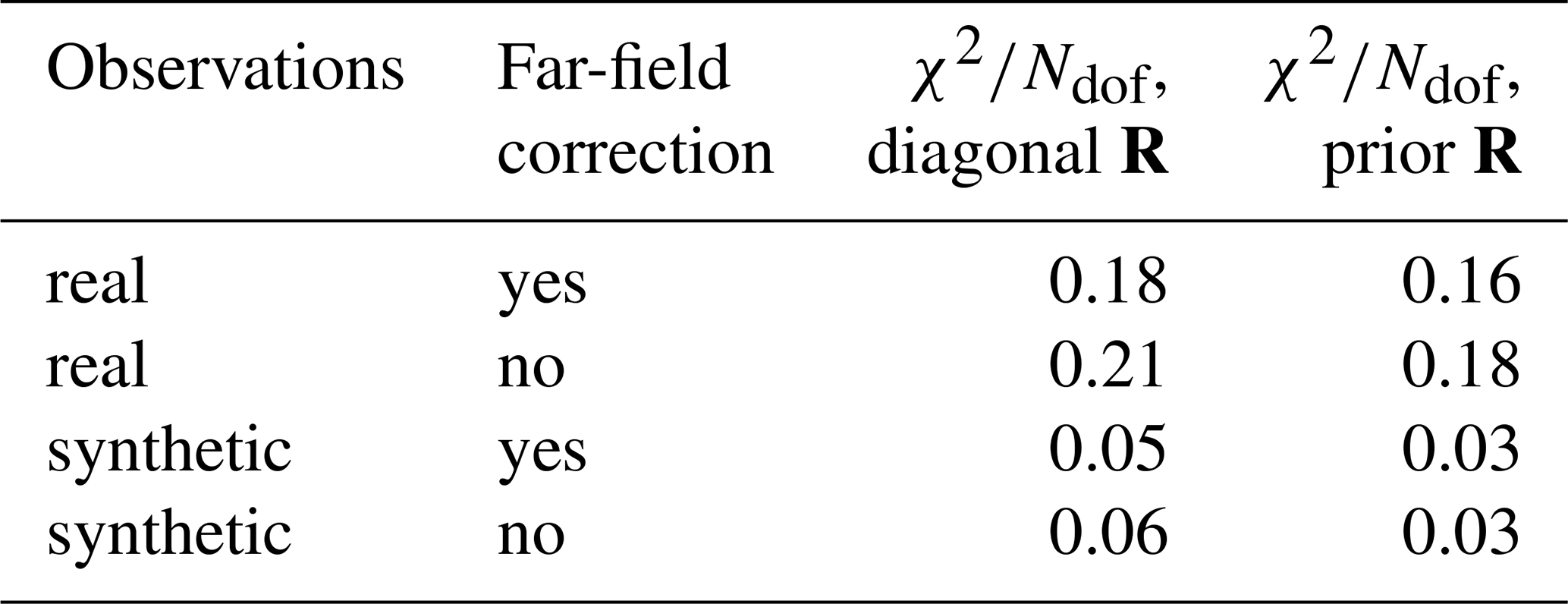
In the synthetic experiments, the idealized transport uncertainty and perfect a priori emissions lead to even lower χ², which is expected because not all uncertainties are contained in the pseudo-observations of these synthetic experiments. Computing ${\mathit{\chi }}^{\mathrm{2}}/N_{\text{dof}}$ for the posterior R inversion is more difficult, but the result is expected to be similar to the prior R inversion. The tuning parameters of the diagonal R matrix were chosen such that the posterior uncertainties are similar to the prior R inversion, which also leads to similar ${\mathit{\chi }}^{\mathrm{2}}/N_{\text{dof}}$ (see Table 2).

2.7 Inversion time window and temporal aggregation

We simulate the transport for the whole year 2021 without any interruption. The inversion is then applied to each month separately by selecting only observations within 1 month. The scaling factors of the months are treated as independent, each month starting with the same a priori scaling factors (${\mathit{s}}_k^{\text{prior}}=\mathrm{1}$ for all k) and the same a priori scaling uncertainties (B matrix). The continuous transport simulation over the whole year implies that the initial CH₄ concentration is hardly relevant after the spin-up. At the beginning of each month, the modeled CH₄ concentration already consists of the far field – the contribution of the lateral boundaries – and the contribution of the fluxes, which will be adjusted by the inversion.

In summary, we correct the contribution of the lateral boundaries on the time scale of 16 h by the far-field correction, and the fluxes on the time scale of 1 month defined by the inversion time window. The inversion results consist of one vector s^post∈ℝ⁴⁶ of scaling factors and the corresponding error covariance matrix for each month. When aggregating results for the whole year, we treat the uncertainties of the prior or posterior fluxes of different months as correlated because these likely include systematic uncertainties and biases which we cannot fully separate from the statistical uncertainty. We therefore aggregate by adding up absolute emissions and their uncertainties linearly.

2.8 Prior uncertainties

In each inversion time window, we consider a priori scaling factors with a two standard deviation (2σ) uncertainty of 0.8 for most flux categories, corresponding to a 95 % confidence interval of ±0.8. Throughout this paper, uncertainties will denote two standard deviations or 95 % confidence intervals. Categories resolving emission sectors have a higher prior 2σ uncertainty of 1.0, and within Germany categories describing the same sector have an a priori uncertainty correlation of 0.5 (e.g., uncertainties of agriculture emissions in the German states of Bavaria and Baden-Wuerttemberg are assumed to be correlated). All other categories are treated as uncorrelated in the a priori. For the Upper Silesian Coal Basin as well as regions with low observation density outside of our primary focus in Central Europe (marked “remote” in Table 1), the 2σ uncertainty is set to 0.5.

3 Input data and processing

We apply the method to estimate CH₄ fluxes in the year 2021 in Germany and in the surrounding European domain, relying on input data for the transport simulation, CH₄ concentration on the lateral boundary (Sect. 3.1), a priori fluxes (Sect. 3.2), and observations (Sect. 3.3).

3.1 Initial and lateral boundary conditions

The meteorological initial and lateral boundary conditions used to drive our transport model are taken from the archive of DWD's operational NWP, which also employs the ICON model. As we do not assimilate meteorological data in our application, we re-initialize the meteorological fields every night at 00:00 UTC, using the analysis fields from the operational NWP data assimilation. Lateral boundary conditions for the meteorological fields are taken from the NWP short term forecasts with hourly resolution.

For the CH₄ concentrations, we use initial and lateral boundary concentrations from the CAMS global inversion-optimized dataset (Segers and Houweling, 2020), version v22r2, in the variant based on surface air-sample data for the inversion. The CAMS data have a resolution of 1°×1° and are interpolated onto our model grid. In contrast to the meteorological fields, the CH₄ concentrations are only transported and never re-initialized. Each transport ensemble member uses slightly different initial and lateral boundary conditions for meteorological fields (see Sect. 2.1.2), but equal CH₄ concentrations on the lateral boundaries.

3.2 A priori CH₄ fluxes

For the inversion, we employ a priori CH₄ fluxes that were compiled from six datasets of anthropogenic and natural fluxes, as detailed in Table 3. We ensured mass conservation when interpolating to our model grid. We generally distinguish between anthropogenic emissions excluding LULUCF, and natural fluxes plus LULUCF. Since the input datasets for anthropogenic emissions are based on reporting to the UNFCCC, these distinguish between GNFR sectors following the reporting conventions (Veldeman et al., 2013). For the inversion, we combine these sectors and only distinguish between agriculture and the sum of all other sectors as described in Sect. 2.1.3. Natural plus LULUCF fluxes of CH₄ are mostly dominated by wetland emissions, for which we do not distinguish between natural and anthropogenic origin.

(UBA, 2023)(Kuenen et al., 2021, 2022)(Segers and Houweling, 2020)Rocher-Ros et al. (2023)Weber et al. (2019)

Table 3 Input data for a priori CH₄ fluxes. The second column lists where these fluxes were considered. Here, “Germany” refers to all model grid cells that lie fully within the German borders. The national reporting distinguishes emissions by GNFR sectors of which A–M include all anthropogenic emissions excluding land use, land use change and forestry (LULUCF).

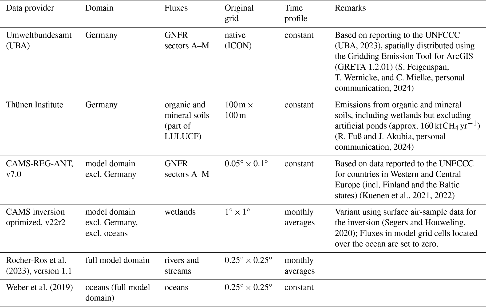
For Germany, we obtained a priori fluxes directly from the national inventory agencies. The a priori LULUCF fluxes obtained from the Thünen Institute cover the emissions from mineral and organic soils. Notably, this excludes emissions from artificial water bodies in Germany – such as ponds – amounting to 160 kt or 8.5 % of the total German emissions in the national reporting, though these numbers are associated with large uncertainties (UBA, 2024, Table 399). These emissions are missing in our a priori estimate, leading to a low bias in the a priori.

3.3 Observations and pre-processing

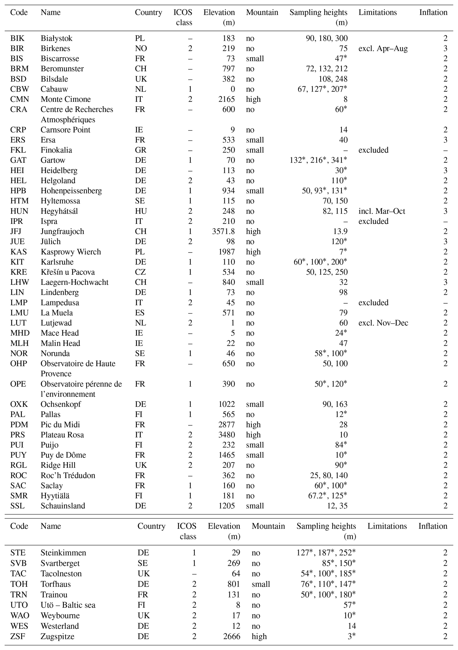
We compare our model predictions to the high quality ground-based in situ observations of CH₄ concentrations collected in the European Obspack (ICOS RI et al., 2024), which includes the ICOS stations among others. These observations are assumed to be representative for a larger area (Storm et al., 2023). Table C1 lists all 53 available stations and Fig. 1 shows 50 stations that were used for the inversion. For tower observations, we use up to three sampling heights per station, preferring the highest three sampling heights and discarding observations below 50 m above ground level to reduce the influence of very local emissions. Due to significant model–observation mismatch, we exclude the IPR, FKL and LMP stations. For LUT, BIR and HUN we only consider some seasons, specified in Table C1.

The model data are interpolated horizontally and vertically to the station sampling locations. The vertical sampling locations in model coordinates are derived from the station sampling heights and the modeled station elevations, depending on the station characteristics (column “mountain” in Table C1). For high mountain stations, the modeled station elevation is given by the real station elevation above mean sea level. For stations on smaller mountains, we consider the arithmetic mean between real station elevation and model topography as proposed by Brunner et al. (2012) and Henne et al. (2016), and for all other stations the modeled station elevation is set to the model topography.

To make use of observations which are likely well represented by the model, we filter the observations based on the local time of day, wind speed, and model–data mismatch. Table 4 lists how the root mean square error (RMSE) of the model output changes during these pre-processing steps. We start by smoothing both observations and modeled concentrations in a time window of approximately ±1.5 h around each observation time as depicted in Fig. 3. This allows for some uncertainty in the timing of modeled tracer transport. The resulting correlation of neighboring time steps is automatically considered in the ensemble-based uncertainty estimate.

Table 4 Average root mean square error (RMSE in ppb), mean absolute bias of the model prediction minus observation (in ppb), and number of available data points after each processing step (1–6) for synthetic (left) and real observations (right). Each row adds a processing step to all previous steps and improves the RMSE. Three numbers for steps 7 and 8 distinguish diagonal R, prior R, and posterior R inversion. Step 7 (uncertainty weighting) is not a processing step in the inversion since it uses only the diagonal of the uncertainty matrix R, but it underscores the importance of accurate uncertainty estimation. Step 8 refers to the result of the inversion. RMSE and absolute bias are computed separately for each station, sampling height and month. The obtained values are weighted by the number of data points and averaged. By taking the mean of multiple RMSEs for different stations, sampling heights and months, we obtain lower numbers than for the RMSE of the combined dataset, which would average squared values and thereby would give higher weight to large deviations between model and observations.

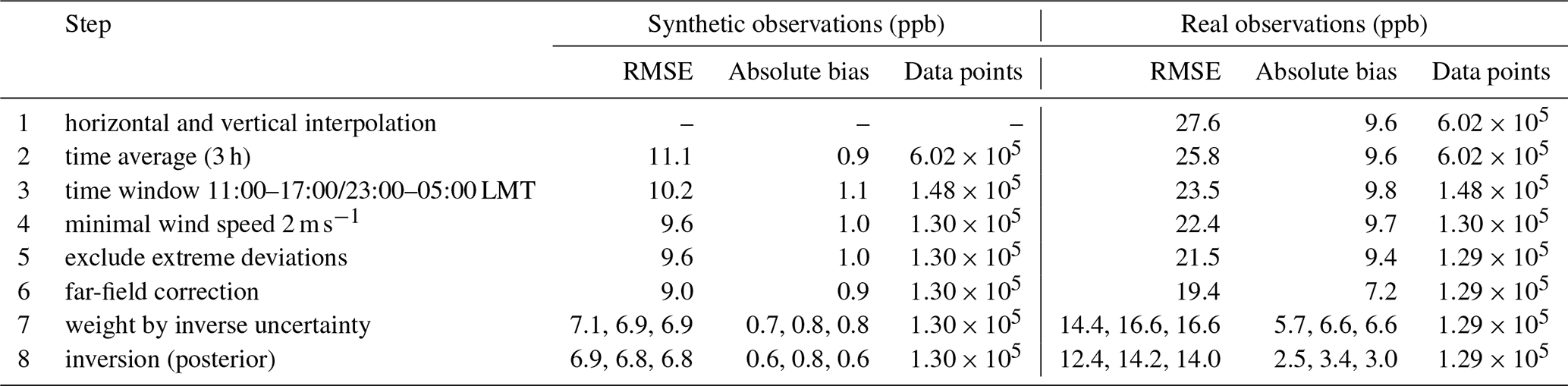
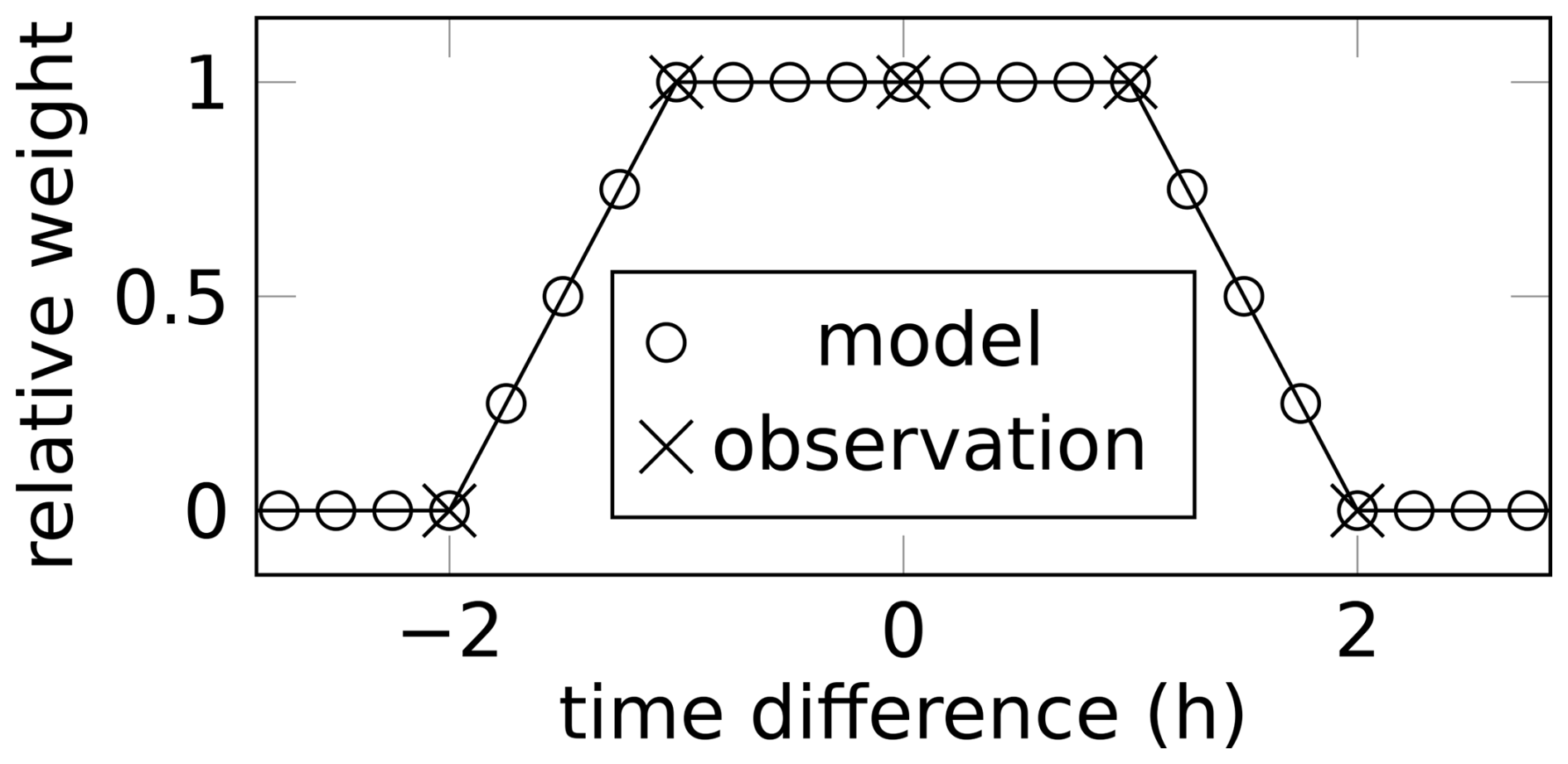
Figure 3 Weighting function for time interpolation of model and observations. For example, an interpolated model point at 16:30 UTC averages over all model output between 15:30 and 17:30 UTC with full weight and another 1 h with linearly decreasing relative weight. The model yields instantaneous values every 15 min, whereas observations are provided as hourly averages, three of which contribute to the observational time average. Reference times are those times for which observations are available.

In the next steps, we filter the data by time in order to keep only observations expected to be representative for large regions. Observations within the planetary boundary layer are most representative in the afternoon hours whereas measurements at high mountains are less influenced by very local fluxes at night time. Inversions therefore commonly use afternoon observations for flat land stations and night times at mountain sites (Bergamaschi et al., 2015; Steiner et al., 2024b). We use the time windows 23:00 to 05:00 LMT (local mean time) for stations on high mountains and 11:00 to 17:00 LMT for all other stations.

We furthermore exclude times with no wind to avoid a strong influence of local emissions that are not resolved in the model, motivated by Ganesan et al. (2015). All data points for which the model predicts a wind speed of <2 m s⁻¹ are excluded, which improves the overall agreement of model and observations as shown in Table 4 (step 4). Figure 4 shows that the RMSE indeed increases significantly at low wind speeds. This increase is partially captured by an increase of the ensemble spread, supporting the idea of an uncertainty estimate depending on wind speed as proposed by Bergamaschi et al. (2022).

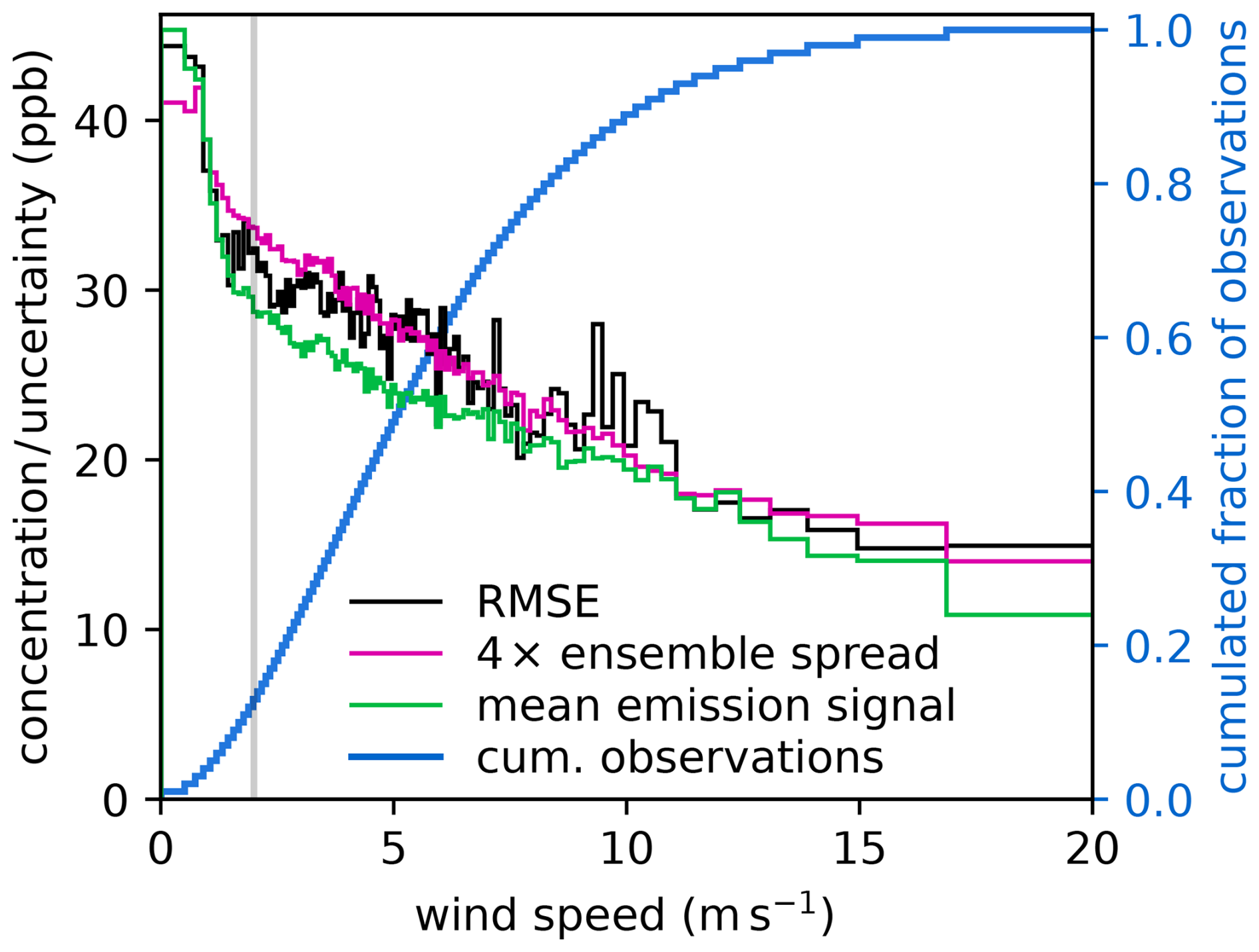
Figure 4 Dependency of RMSE and proxies for the model uncertainty on wind speed (left axis). All data points from step 3 in Table 4 were ordered by the model-predicted wind speed and split into 100 bins, each containing approximately 1500 data points. The blue line indicates the cumulative fraction of observations (right axis). The figure shows the RMSE difference of model and observation (black line), the mean ensemble spread multiplied by factor 4 (red line), and the mean a priori concentration due to categorized emissions (green line) for each of these bins. The ensemble spread is the standard deviation of the model prediction in the 12 ensemble members. It is a main contribution to our uncertainty estimate for the model–data mismatch in the prior R and posterior R inversion. The signal of categorized emissions is used to estimate the uncertainty for the diagonal R matrix. Much of the larger RMSE at low wind speed is well captured by the ensemble spread inflated by factor 4 and by the mean a priori emission signal. In the inversion, we discard data points with wind speeds below 2 m s⁻¹ (gray vertical line).

In the last filtering step – step 5 in Table 4 – we exclude data points with extreme mismatch between far-field corrected a priori and observations, where $|{\mathit{y}}_i-(\mathbf{H}\mathit{s}{)}_i-{\mathit{x}}_i^{\text{ff}}|>\mathrm{200}$ ppb. Data points where ${\mathit{y}}_i-{\mathit{x}}_i^{\text{ff}}<-\mathrm{20}$ ppb are also discarded. Since no strong sinks of CH₄ are expected, the contribution of CH₄ from the lateral boundaries should not exceed the observations. Thus, an observation below the model-predicted far field indicates an error in this far field. Steps 6–8 in Table 4 complete our processing chain by applying the far-field correction (Sect. 2.3), indicating the relevance of the model uncertainty (Sect. 2.5 and 2.6), and finally using the inversion results.

3.4 Synthetic observation experiments

To test our setup and analyze biases, we use synthetic experiments in which observation data are replaced by model-generated pseudo-observations. These synthetic experiments use exactly the same setup and the same observation coordinates. Only the observation values are replaced by the simulation result of one of our 12 ensemble members. We thus obtain 12 separate datasets of pseudo-observations, in which a transport error is simulated by using the transport ensemble members. The true fluxes assumed for these synthetic experiments are identical to the prior fluxes. This allows us to estimate a bias and a random error in the posterior scaling factor. We will repeat this procedure with modified true fluxes in Sect. 4.3. An analysis of the sensitivity to random changes in the true fluxes is included in Part 2 (Bruch et al., 2025a).

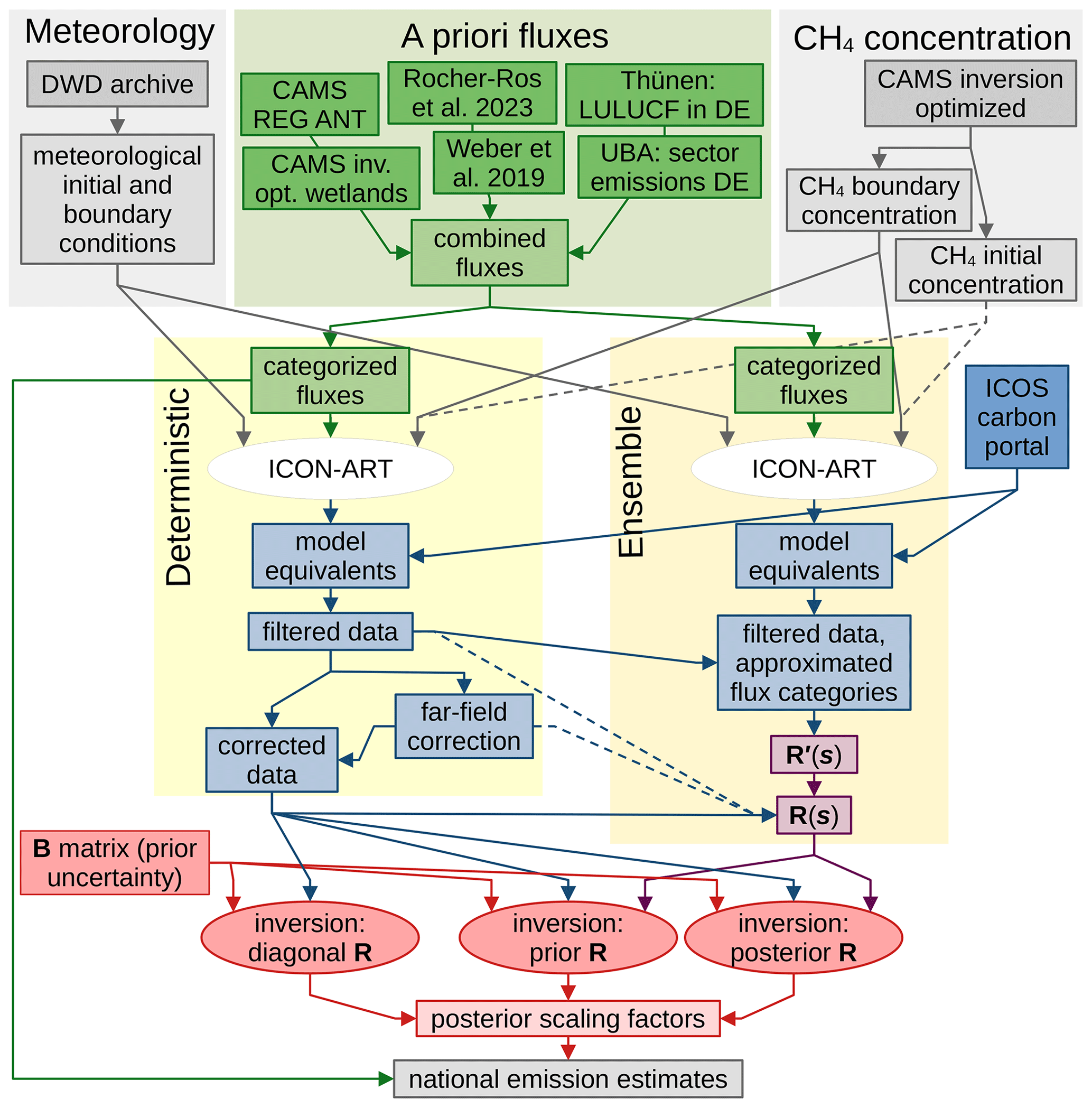
Figure 5 Overview of the inversion system including input data sources. Arrows indicate data streams. Dashed lines indicate data streams with small or negligible impact on the inversion results. Colored areas group the input data (top), the deterministic model run and data processing (left), and the ensemble model run including processing of the resulting data (right). Colored text boxes distinguish gridded fluxes (green), data in observation space (blue, matrices in purple), and data in the space of scaling factors (red). Observation data are included when working in observation space (not explicitly marked). At the end of the processing chain (bottom), the three methods for estimating R lead to different scaling factors from which we can compute national emission estimates.

3.5 Summary and overview

We can now summarize the inversion method following the required data streams in Fig. 5. After collecting the input data for the transport simulation (Sect. 3.1 and 3.2, top of Fig. 5), we prepare the inversion by categorizing the fluxes (Sect. 2.1.3). The transport is simulated separately for the deterministic and ensemble run (Sect. 2.1.1, white ellipses in Fig. 5). Using observation data from the ICOS carbon portal and the simulation output, we compute model equivalents and filter these to ensure a high quality of the model predictions (Sect. 3.3). The data from the deterministic run are used to construct a far-field correction to mitigate uncertainties in the boundary conditions (Sect. 2.3). The ensemble data are used to construct the uncertainty matrix R(s) as required for the prior R and posterior R inversion (Sect. 2.5.2). The far-field corrected data and the R matrix serve as input for the Bayesian inversion (Sect. 2.4). By combining the resulting posterior scaling factors with the categorized fluxes, we obtain posterior flux estimates.

4 Results and discussion

In this section, we examine the presented inversion system using synthetic experiments and sensitivity tests. We start by considering synthetic observation experiments in which the synthetic truth is equal to the a priori fluxes. Figure 6 shows a statistical evaluation of inversion results for this case, which we analyze for multiple aspects.

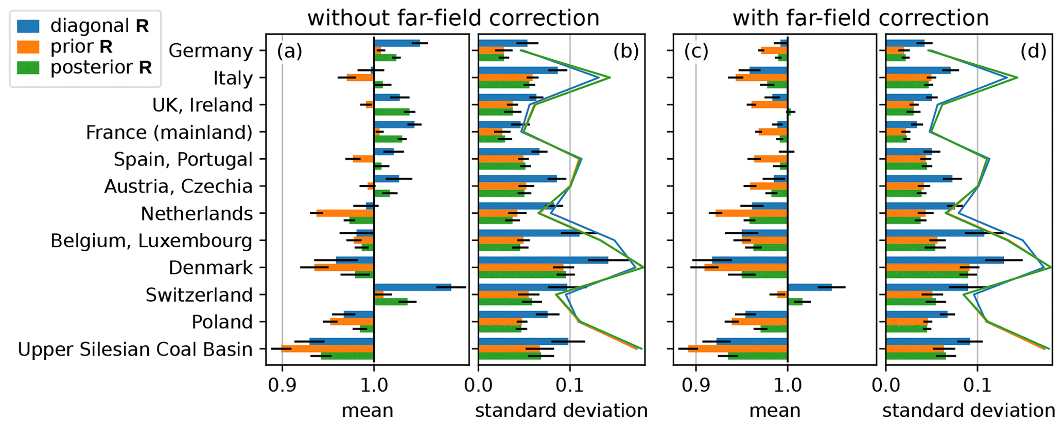
Figure 6 Mean (a, c) and standard deviation (b, d) of monthly flux estimates relative to the prior in synthetic experiments for diagonal R (blue), prior R (orange), and posterior R inversion (green). Each bar represents the posterior fluxes for 144 inversions, obtained from 12 datasets of pseudo-observations, each covering 12 monthly time windows. Black horizontal lines indicate the 2σ statistical uncertainty estimate. Panels (a), (c) show the bias as the relative deviation of the mean posterior from the prior, which is equal to the synthetic truth. The standard deviation (b, d) among the 144 emission estimates indicates the random error expected in each monthly inversion. Colored lines in (b), (d) show the mean posterior 1σ uncertainty, which is similar for all three methods.

4.1 Random error

In Fig. 6, we see the bias (panels a and c) and random error (b and d) of the inversion results for selected countries or emission sources relative to the a priori emissions, distinguishing the three methods for constructing R. The random error is estimated by the standard deviation obtained from 144 inversions and indicates the precision or reliability of these results for a single month. The comparison of the three methods shows that the prior R and posterior R method lead to a very similar random error, which is considerably lower than for the diagonal R in all considered regions. This leads to the conclusion that using a transport ensemble to estimate uncertainties and their correlations can significantly reduce the random error in emission estimates, independent of the far-field correction.

Since the diagonal R construction uses different tuning parameters than the prior R and posterior R inversion, we need to make sure that the chosen configurations are comparable. This is achieved by aiming for a similar posterior uncertainty in all methods for constructing R. Thin lines in Fig. 6b and d show the posterior 1σ uncertainties to validate the similarity.

By comparing emission estimates without (panels a and b) and with the far-field correction (c and d), one can identify that the far-field correction changes the bias and slightly reduces the random error. Both effects are very similar for all three choices of R. Since the far-field correction pulls the simulated prior concentrations towards the observations, we can expect that it brings the emission estimates closer to the prior. But we can see in Fig. 6b and d that the resulting reduction in random error is only weak.

4.2 Inversion bias

The bias shown in Fig. 6a and c clearly depends on the far-field correction. The pseudo-observations without far-field correction have a bias of +0.5 ppb. The far-field correction reverts this to a negative bias of −0.5 ppb due to a sampling bias as explained in Sect. 2.3. Ideally, we would therefore expect a small positive bias in Fig. 6a and an equally strong negative bias in panel (c). But the bias differs depending on how R is constructed.

For the diagonal R inversion, we see overall a positive bias for most regions. This approximation for R assumes a large uncertainty if the model predicts a strong signal from emissions. For an imperfect transport model, this implies that the model will tend to have a higher uncertainty when it overestimates the concentration and a lower uncertainty when it underestimates the real emission signal. As the model is more confident when observations are higher than the model prediction, it will tend to overestimate the emissions.

For the prior R approximation, we find a negative bias in the emission estimates in many regions. This may be due do the plume bias problem introduced in Sect. 2.2. For the Upper Silesian Coal Basin as a very strong and localized source, all methods show the expected negative bias. Notably, a considerable negative bias is also found for the Netherlands as a small country with high emission rates.

In the posterior R approximation, the negative bias for plumes is reduced, but also all other emission estimates are higher compared to the prior R inversion. To understand this, we recall that a transport error in our model only leads to an error in the predicted CH₄ concentration if the concentration field contains spatial gradients. Such gradients are caused by emissions. Stronger emissions directly cause higher uncertainty estimates in the meteorological ensemble. In the posterior R inversion, the inversion can adjust the emissions of the transport ensemble and thereby change the uncertainties. As we optimize the agreement of model and observations relative to the uncertainties, the system will prefer larger uncertainties. Thus, the inversion will tend to overestimate emissions to reach higher uncertainties. This counteracts the negative plume bias, but it may also lead to a positive bias.

By combining bias and random error, we obtain the RMSE. For Germany, the monthly results with far-field correction show an RMSE between 2.4 % (posterior R) and 4.3 % (diagonal R). For yearly totals, this reduces to 1.2 % for posterior R and 1.8 % for diagonal R, while the prior R inversion is dominated by the bias and has an RMSE of 2.9 %. This indicates that the simulated transport error in our synthetic experiments leads to an error of approximately 2 % on the German yearly total emission estimate. Overall, the posterior R inversion shows the best performance as it has a lower random error and only a small bias.

4.3 Sensitivity to increased true emissions

To test the sensitivity of the inversion to true fluxes, we repeat the synthetic experiments with an identical setup but different pseudo-observations. For these new pseudo-observations, we increase all anthropogenic emissions by 20 %. The a priori emissions remain unchanged and are thus lower than the synthetic truth. The inversion results are summarized in Fig. 7, which is analogous to Fig. 6.

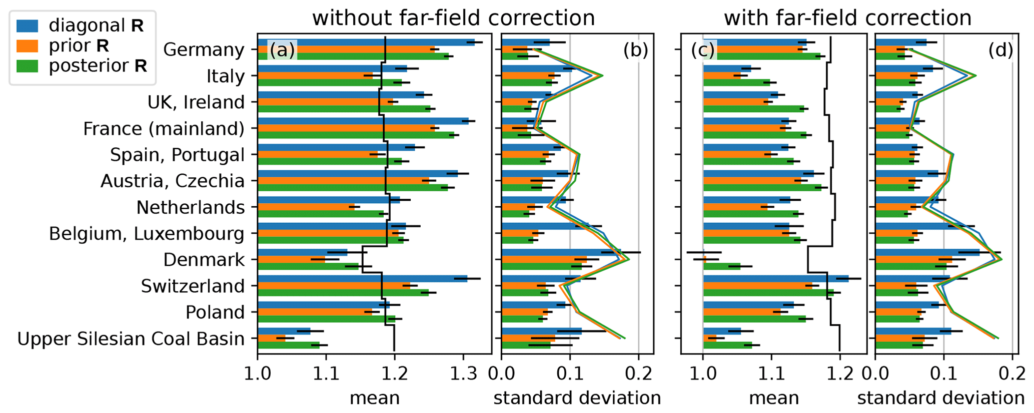
Figure 7 Mean (a, c) and standard deviation (b, d) of monthly flux estimates relative to the prior in synthetic experiments with 20 % increased anthropogenic emissions in the synthetic truth for diagonal R (blue), prior R (orange), and posterior R inversion (green). In (a, c), the a priori has value 1.0 and a black vertical line shows the synthetic truth. Bars connect the prior to the posterior. Like in Fig. 6, each bar represents the posterior fluxes for 144 inversions, combining 12 months with 12 datasets of pseudo-observations. Horizontal lines show 2σ statistical uncertainties and colored lines in (b), (d) indicate the posterior 1σ uncertainty.

Figure 7a and c show the mean posterior (bars) compared to the synthetic truth (black vertical line). Without the far-field correction, the inversion is too sensitive in many regions, as it increases the emissions beyond the synthetic truth. This leads to an overestimation, which is likely due to the artificial lifetime of the flux category tracers (see Sect. 2.1.4). With the far-field correction (panel c), the deviation of the posterior from the prior is damped and we obtain a low bias compared to the truth, as expected when the a priori emissions are underestimated. The random error (b and d) remains similar to the case with perfect prior emissions, albeit a small increase can be seen (compare Fig. 6). Like for the perfect prior emissions, the best performance with the lowest RMSE is found for the posterior R inversion.

4.4 Sensitivity to bias and noise in observations

We now turn from the focus on the transport error to uncertainties in the observations. To this end, we consider different pseudo-observations without any transport error that follow scenarios defined in Fig. 8. To avoid the transport error, we generate these pseudo-observations based on the deterministic model run. For simplicity, we only consider the average of prior R and posterior R inversion.

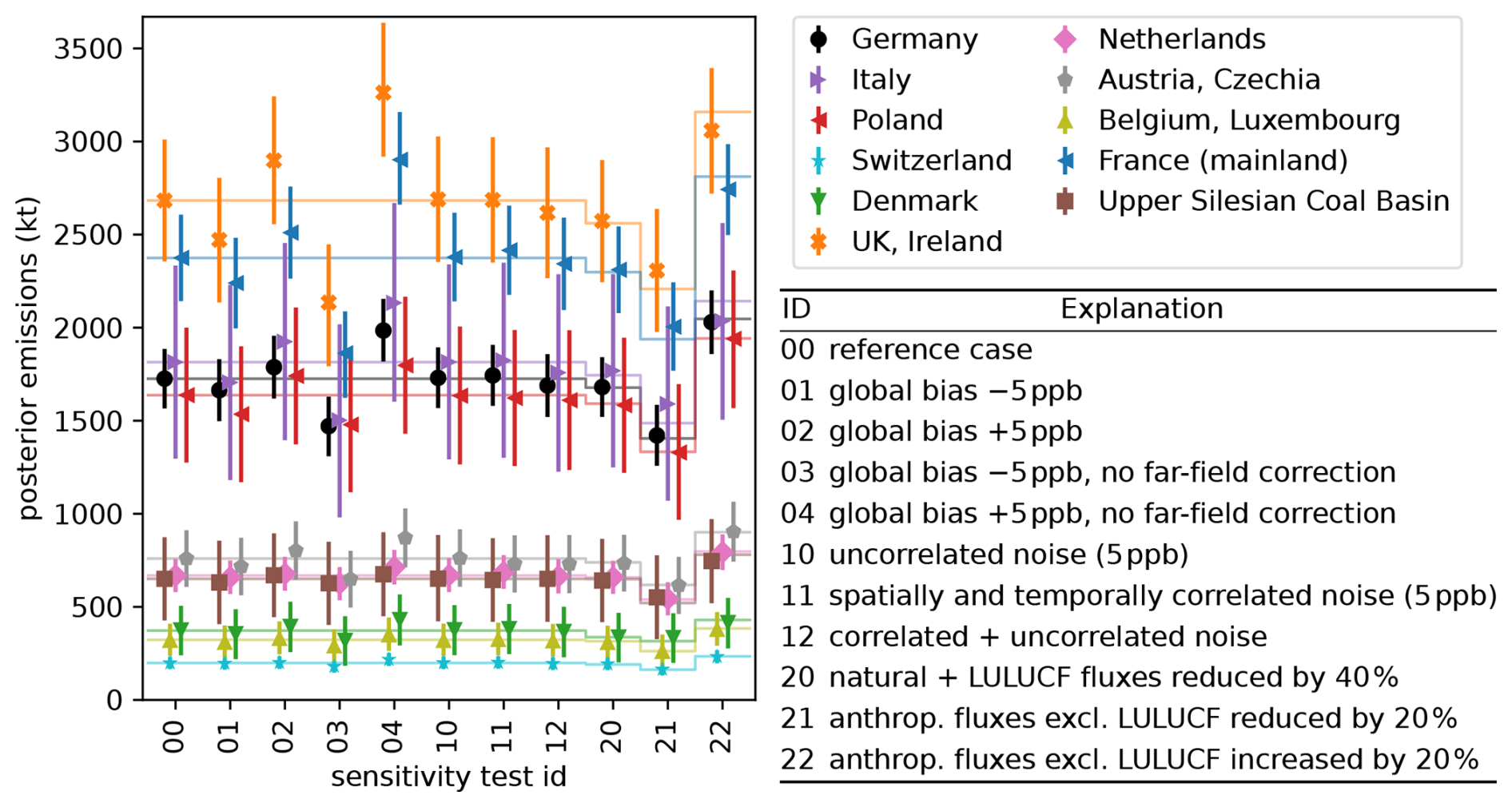
Figure 8 Total posterior emissions in 2021 of selected countries and German sectors for synthetic experiments with perfect transport. Markers show the average of the emission estimates obtained from the prior R and posterior R inversion. Thin horizontal lines indicate the synthetic truth. Vertical lines show uncertainties (95 % confidence intervals).

In the first scenarios, we shift all pseudo-observations by −5 ppb (case 01 in Fig. 8) and +5 ppb (case 02). This bias is mostly compensated by the far-field correction with monthly averages of ±2.75 to ±3.8 ppb, the sign depends on the scenario. Because of this correction, the effect on the estimated German total emissions remains well within the posterior uncertainty. This is in stark contrast to the same scenarios without the far-field correction (cases 03 and 04) and demonstrates the benefits of the far-field correction.

We furthermore test the effect of correlated and uncorrelated Gaussian noise added to the observations (cases 10–12), finding that the effect on the posterior emissions is small compared to the posterior uncertainties. The correlated Gaussian noise is a three-dimensional Gaussian random field in flat (longitude, latitude, time) coordinates with a lower cutoff for fluctuations on scales ≲2.5° (horizontal) and ≲12 d (time) such that it acts as a slowly varying random bias. The RMS of the noise is normalized to 5 ppb. For the last three test cases (20–22), we scale either the natural and LULUCF fluxes or all other emissions in the synthetic truth while leaving the a priori emissions unchanged. Overall, the emission estimates follow the change in the synthetic truth well as already found in Sect. 4.3.

4.5 Sensitivity to inversion parameters

Our inversion method has various tuning parameters. Above we have described the inversion and synthetic experiments for one choice of these parameters. We analyze the sensitivity to these parameters by repeating the inversion 50 times with real observations and modified parameters. Table E1 lists these test cases with their ID, parameters, and influence on the inversion results. An overview of the national emission estimates for each test case is provided in Fig. E1. Here, we summarize the main results and refer to Table E1 for details. We use the average of the prior R and posterior R inversion results and focus on the influence of the parameters on the emission estimates, leaving the discussion of the inversion results for Part 2 (Bruch et al., 2025a).

4.5.1 Comparison to observations

Before comparing model and observations, we apply multiple filtering steps that influence the inversion results considerably. Most prominently, selecting nighttime observations for high mountain stations and afternoon hours for other stations strongly affects the inversion and improves the model representativeness (case 201 in Table E1). This is one of only five sensitivity tests with posterior fluxes deviating from the reference case by ≳30 % of the posterior uncertainty, which we call a strong change in inversion results. Other filtering parameters such as the number of sampling heights used per station (case 202) and the minimal wind speed (cases 203–205) affect the inversion results noticeably, although changes are small compared to the uncertainties. Limiting the influence of outliers with model–observation mismatch $\left|{\mathit{\mu }}_i\right|>\mathrm{3}\sqrt{{\mathbf{R}}_{ii}^{\prime }}$ by increasing their uncertainty (see Sect. 2.6.2) has a considerable impact (cases 208, 209). Completely neglecting extreme outliers – defined by $|{\mathit{y}}_i-(\mathbf{H}\mathit{s}{)}_i-{\mathit{x}}_i^{\text{ff}}|>\mathrm{200}$ ppb or ${\mathit{y}}_i-{\mathit{x}}_i^{\text{ff}}<-\mathrm{20}$ ppb – has only a small effect (cases 206, 207).

The choice of observation sites is analyzed in cases 601 and 602, which select subsets of stations with good observation coverage over the full year. When using only 27 stations (case 602), the results change strongly compared to the reference case with 50 stations, also because some regions are hardly observed in case 602. Varying the elevation of high mountain stations has only little impact on the inversion results (case 100). The effect of time-averaging over 3 h (as chosen in step 2 of Sect. 3.3) is noticeable in the results, but small compared to the uncertainties (case 101).

4.5.2 Uncertainty

The diagonal R inversion deviates from the reference case by one third of the posterior uncertainty (case 311). Also the construction of the error covariance matrix R following Sects. 2.5 and 2.6 contains numerous tuning parameters. Key parameters are the overall uncertainty inflation factors f_i (Sect. 2.6.3, cases 302 and 303 in Table E1) and the uncorrelated additive uncertainty σ_const (see Eq. 2) of each data point (cases 309, 310). Variations of these parameters change the inversion results considerably. The tuning parameter σ_const illustrates the importance of hidden patterns in the considered data. Increasing to σ_const=20 ppb effectively reduces the weight of observations with a small ensemble-estimated transport uncertainty. As observations with strong emission signals and high transport uncertainty become more relevant, the emission estimate for Germany is increased by 5 % (case 310 in Fig. E1).

Other important parameters are the correlation scales in the localization matrix C for the ensemble-based uncertainty estimate (see Sect. 2.5.2). The overall effect of these scales on the posterior scaling factors is small (cases 304–308), but these parameters also influence the posterior uncertainties. The sensitivity tests indicate that 12 ensemble members are sufficient to estimate the uncertainties and correlations even without a strong localization. In general, we expect that a larger transport ensemble will yield better statistical estimates for uncertainties and their correlations. This reduces the need for a localization which suppresses spurious correlations. The considered additional plume localization uncertainty (see Sect. 2.6.1, cases 300 and 301) arising from the Upper Silesian Coal Basin seems negligible when considering the full domain. However, the additional plume localization uncertainty reduces the negative bias for the plume emissions that was discussed in Sect. 2.2.

4.5.3 Far-field correction

The synthetic experiments already showed that the far-field correction introduced in Sect. 2.3 influences the results considerably (see Figs. 6 and 7). When using real observations, removing the correction field leads to strong changes in the inversion results (case 400), albeit the results remain within the posterior uncertainty bounds. Without the correction, the scaling factors for some natural fluxes in Scandinavia even become negative for some months – a clearly unrealistic result that underlines the importance of the far-field correction. However, changing various tuning parameters of the far-field correction within a reasonable range has much smaller effects. The selection of data points used for the far-field correction (cases 409, 410) and the overall correction strength (cases 401, 402) have modest influence, whereas correlation scales in the correction play a minor role (cases 403–408). The additional uncertainty added to R due to the far-field correction (see Sect. 2.6.4) has little influence on the inversion results (cases 412–414).

4.5.4 A priori error covariance matrix

Modifying the a priori uncertainty or correlations of the scaling factors (B in Eq. 1) changes the results quantitatively, but not qualitatively (cases 500–502). A coarser spatial resolution in Germany (case 504) and different choices of sectors (cases 503, 506) yield aggregated German sector emissions that agree well with the reference case.

4.5.5 Inversion time windows

In the reference case, we considered each month independently. Increasing the inversion time windows to 3 months has a considerable influence on the results (case 702). As the inversion time window increases, the overall weight of the observations in the inversion also increases. Thus, posterior uncertainties are reduced and the deviations between posterior and prior are amplified.

5 Conclusions

This study introduced a new flux inversion system that explores the potential of a transport ensemble from NWP for observation-based regional estimation of methane emissions. In experiments with pseudo-observations and simulated transport error, we found that using a transport ensemble can substantially reduce the random error of the flux estimates compared to a simple baseline scenario (“diagonal R”). This is in line with findings by Ghosh et al. (2021) and by Steiner et al. (2024a), who estimated CH₄ emissions in Europe using an ensemble Kalman smoother. But in contrast to Ghosh et al. (2021), who studied CO₂ at urban scale using an ensemble transform Kalman filter, we identified no significant improvement in the bias of the emission estimates. Instead, our results indicate systematic biases depending on the emissions characteristics. Most notably, localized sources causing strong plumes can be underestimation by 10 % by our synthesis inversion. To benefit from the transport ensemble and to reduce such biases, we proposed to use the posterior concentrations in the ensemble when constructing R. This posterior R inversion showed the best performance in the synthetic experiments. Overall, we expect an error of 2 % for the total German CH₄ emissions in 2021 in our inversion system due to random transport errors.

When applying our regional inversion system to real observations, we face the challenge of uncertain CH₄ concentrations at the lateral boundaries. Different approaches exist to correct biased boundary conditions. In some cases, selected measurements can provide a baseline (Lauvaux et al., 2013). At national or continental scale, a coarse discretization of the boundaries allows optimization along with the emissions (Ganesan et al., 2015; Steiner et al., 2024b). Here, we followed a different path by adding a smooth correction field for the simulated concentrations. This allowed us to use different time scales for the inversion and the far-field correction. The far-field correction causes a small bias towards the prior fluxes, but without the correction we expect errors from wrongly projecting any boundary bias onto the fluxes. We demonstrated the potential of the far-field correction using biased pseudo-observations and analyzed its importance in sensitivity tests, for which we repeated the inversion with different tuning parameters. These tests with real observations show that switch on the far-field correction changes the results considerably within the uncertainty ranges, but the specific choices made in constructing the correction field have only minor or moderate effects. Also other tested changes in tuning parameters only lead to variations of the full-year flux estimates well within the uncertainty ranges, indicating that we found robust settings for our application. This establishes a basis for applying our system to validate the German emission inventory in Part 2 (Bruch et al., 2025a).

The presented novel inversion system leverages the potential of the ICON–ART model and the ensemble modeling capabilities from operational NWP for national scale estimation of CH₄ fluxes. It is tailored to the validation of national inventories by using high-resolution a priori emission estimates from national reporting and allowing for distinguishing emission sectors, as will be discussed in detail in Part 2. With synthetic experiments and sensitivity tests we demonstrated the suitability for estimating national CH₄ emissions.

Appendix A: Formal definition of far-field correction

This appendix provides details for the far-field correction introduced in Sect. 2.3. We correct the computed far field by a smooth field that is determined using all data points where the cumulated signal of all flux categories is at most 20 ppb, the total concentration due to all fluxes in the domain – including natural and uncategorized fluxes – is at most 50 ppb, and natural plus LULUCF fluxes contribute at most 20 ppb. These criteria aim to select only measurements of sufficiently clean air for the far-field correction.

The far-field correction is realized as a Kalman smoother on the selected data points. For simplicity, we only provide the definition of the correction at the observation coordinates. Consider the vector of all model predictions x, which is aligned with the observation vector y. By P we denote the projector selecting those data points that shall be used to determine the far-field correction. We aim to find a correction vector c aligned with x and y that minimizes

$$\begin{array}{}\text{(A1)}& \begin{array}{rl}\underset{\mathit{c}}{\text{arg\hspace{0.17em}min}}\mathit{\{}& \frac{\mathrm{1}}{\mathrm{2}}(\mathit{x}+\mathit{c}-\mathit{y}{)}^{\top }{\mathbf{P}}^{\top }(\mathbf{P}\stackrel{\mathrm{̃}}{\mathbf{R}}{\mathbf{P}}^{\top }{)}^{-\mathrm{1}}\mathbf{P}(\mathit{x}+\mathit{c}-\mathit{y})\\ & +\frac{\mathrm{1}}{\mathrm{2}}{\mathit{c}}^{\top }{\mathbf{P}}^{\top }\left(\mathbf{P}\stackrel{\mathrm{̃}}{\mathbf{C}}{\mathbf{P}}^{\top }{)}^{-\mathrm{1}}\mathbf{P}\mathit{c}\mathit{\right\}},\end{array}\end{array}$$

where $\stackrel{\mathrm{̃}}{\mathbf{R}}=\mathrm{16}\mathbf{I}$ is a diagonal matrix and $\stackrel{\mathrm{̃}}{\mathbf{C}}$ a Gaussian localization matrix with standard deviations 16 h (time), 319 km (horizontal) and 1 km (vertical), normalize to ${\stackrel{\mathrm{̃}}{\mathbf{C}}}_{ii}=\mathrm{1}$ for all i. The matrix $\stackrel{\mathrm{̃}}{\mathbf{C}}$ ensures that the correction field c is smooth on these scales. For the under-determined Eq. (A1) we use the solution

$$\begin{array}{}\text{(A2)}& \mathit{c}=\stackrel{\mathrm{̃}}{\mathbf{C}}{\mathbf{P}}^{\top }\left[\mathbf{P}\right(\stackrel{\mathrm{̃}}{\mathbf{C}}+\stackrel{\mathrm{̃}}{\mathbf{R}}\left){\mathbf{P}}^{\top }{]}^{-\mathrm{1}}\mathbf{P}\right(\mathit{y}-\mathit{x}).\end{array}$$

This only defines c at the observations, but we can generalize Eq. (A2) to arbitrary locations and times by including these coordinates in $\stackrel{\mathrm{̃}}{\mathbf{C}}$. Formally, this then defines a smooth field.

To prove that Eq. (A2) is one possible – albeit not unique – solution of Eq. (A1), we use that Eq. (A1) is a quadratic form and compute its gradient with respect to c:

$$\begin{array}{}\text{(A3)}& \begin{array}{rl}\mathrm{0}\stackrel{!}{=}& {\mathbf{P}}^{\top }\left(\mathbf{P}\stackrel{\mathrm{̃}}{\mathbf{R}}{\mathbf{P}}^{\top }{)}^{-\mathrm{1}}\mathbf{P}\right(\mathit{x}+\mathit{c}-\mathit{y})\\ & +{\mathbf{P}}^{\top }(\mathbf{P}\stackrel{\mathrm{̃}}{\mathbf{C}}{\mathbf{P}}^{\top }{)}^{-\mathrm{1}}\mathbf{P}\mathit{c}.\end{array}\end{array}$$

Since PP^⊤ has full rank, this implies that

$$\begin{array}{ll}{\displaystyle }\mathrm{0}\stackrel{!}{=}& {\displaystyle }\left[\right(\mathbf{P}\stackrel{\mathrm{̃}}{\mathbf{R}}{\mathbf{P}}^{\top }{)}^{-\mathrm{1}}+\left(\mathbf{P}\stackrel{\mathrm{̃}}{\mathbf{C}}{\mathbf{P}}^{\top }{)}^{-\mathrm{1}}\right]\mathbf{P}\mathit{c}\\ \text{(A4)}& {\displaystyle }& {\displaystyle }+\left(\mathbf{P}\stackrel{\mathrm{̃}}{\mathbf{R}}{\mathbf{P}}^{\top }{)}^{-\mathrm{1}}\mathbf{P}\right(\mathit{x}-\mathit{y})\text{(A5)}& {\displaystyle }⟹\mathbf{P}\mathit{c}=& {\displaystyle }[\mathbf{1}+\mathbf{P}\stackrel{\mathrm{̃}}{\mathbf{R}}{\mathbf{P}}^{\top }(\mathbf{P}\stackrel{\mathrm{̃}}{\mathbf{C}}{\mathbf{P}}^{\top }{)}^{-\mathrm{1}}{]}^{-\mathrm{1}}\mathbf{P}(\mathit{y}-\mathit{x})\text{(A6)}& {\displaystyle }=& {\displaystyle }\mathbf{P}\stackrel{\mathrm{̃}}{\mathbf{C}}{\mathbf{P}}^{\top }\left[\mathbf{P}\right(\stackrel{\mathrm{̃}}{\mathbf{C}}+\stackrel{\mathrm{̃}}{\mathbf{R}}\left){\mathbf{P}}^{\top }{]}^{-\mathrm{1}}\mathbf{P}\right(\mathit{y}-\mathit{x}).\end{array}$$

It follows that Eq. (A2) is a solution of Eq. (A1) that is independent of the non-selected data points. One can furthermore show that Eq. (A2) is optimal in the sense that it minimizes ${\mathit{c}}^{\top }{\stackrel{\mathrm{̃}}{\mathbf{C}}}^{-\mathrm{1}}\mathit{c}$ under constraint that c is a solution of Eq. (A1). Thus, this solution is as close as possible to zero under the constraint of smoothness (quantified by $\stackrel{\mathrm{̃}}{\mathbf{C}}$). By defining $\mathit{\xi }=\left[\mathbf{P}\right(\stackrel{\mathrm{̃}}{\mathbf{C}}+\stackrel{\mathrm{̃}}{\mathbf{R}}\left){\mathbf{P}}^{\top }{]}^{-\mathrm{1}}\mathbf{P}\right(\mathit{y}-\mathit{x})$ and introducing Lagrange multipliers λ, we obtain

$$\begin{array}{ll}{\displaystyle }f(\mathit{c},\mathit{\lambda })& {\displaystyle }={\mathit{c}}^{\top }{\stackrel{\mathrm{̃}}{\mathbf{C}}}^{-\mathrm{1}}\mathit{c}+{\mathit{\lambda }}^{\top }(\mathbf{P}\mathit{c}-\mathbf{P}\stackrel{\mathrm{̃}}{\mathbf{C}}{\mathbf{P}}^{\top }\mathit{\xi }),\\ \text{(A7)}& {\displaystyle }& {\displaystyle \frac{\partial f}{\partial {\mathit{c}}_i}}=\mathrm{0},{\displaystyle \frac{\partial f}{\partial {\mathit{\lambda }}_j}}=\mathrm{0},\text{(A8)}& {\displaystyle }\mathit{c}& {\displaystyle }=-\stackrel{\mathrm{̃}}{\mathbf{C}}{\mathbf{P}}^{\top }\mathit{\lambda }\mathrm{\text{from }}{\partial }_{{\mathit{c}}_i}f(\mathit{c},\mathit{\lambda })=\mathrm{0},\text{(A9)}& {\displaystyle }\mathbf{P}\mathit{c}& {\displaystyle }=\mathbf{P}\stackrel{\mathrm{̃}}{\mathbf{C}}{\mathbf{P}}^{\top }\mathit{\xi }\mathrm{\text{from }}{\partial }_{{\mathit{\lambda }}_j}f(\mathit{c},\mathit{\lambda })=\mathrm{0}.\end{array}$$

Since $\mathbf{P}\stackrel{\mathrm{̃}}{\mathbf{C}}{\mathbf{P}}^{\top }$ has full rank, combining Eqs. (A8) and (A9) implies that $\mathit{\lambda }=-\mathit{\xi }$ and thereby $\mathit{c}=\stackrel{\mathrm{̃}}{\mathbf{C}}{\mathbf{P}}^{\top }\mathit{\xi }$ is the unique solution of the optimization problem arg min_cf(c,0) under the constraint that $\mathbf{P}\mathit{c}=\mathbf{P}\stackrel{\mathrm{̃}}{\mathbf{C}}{\mathbf{P}}^{\top }\mathit{\xi }$.

Appendix B: Posterior R with reduced ensemble

When using a priori scaling factors to estimate the model uncertainty in R, we need only the total concentration ${\mathit{x}}_i^m\left({\mathit{s}}^{\text{prior}}\right)$ for each ensemble member m and each observation i, where s^prior is known. Thus, only a single tracer field is required in the ensemble transport simulation. To compute ${\mathit{x}}_i^m\left(\mathit{s}\right)$ for arbitrary s∈ℝ⁴⁶, the flux categories need to be distinguished for each ensemble member, resulting in >40 tracer fields in the ensemble simulation. To avoid wasting numerical resources, we chose to approximate ${\mathit{x}}_i^m\left(\mathit{s}\right)$ by only a few tracer fields, using additional information from the deterministic model run which distinguishes all tracer fields.

From the deterministic model run, we know the operator H mapping scaling factors s to a model prediction Hs+x^ff for the concentrations. For ensemble member m, we would ideally know H^m and x^ff,m to compute a model prediction ${\mathbf{H}}^m\mathit{s}+{\mathit{x}}^{\text{ff},m}$. In lack of computational resources to compute H^m for every ensemble member, we combine information from the deterministic run (H) and selected tracers for the ensemble run to approximate H^m. We group the flux categories into groups {g} and denote by P_g the projector of scaling vectors s on the subspace spanned by the flux categories in group g. In the ensemble members, we compute the total concentration from group g, ${\mathit{x}}_i^{\text{mg}}={\mathbf{H}}^m{\mathbf{P}}_g{\mathit{s}}^{\text{prior}}$. We distribute the 46 flux categories to only three groups and thereby reduce the computational effort considerably. To estimate the full dependence on the scaling factors in the ensemble, we approximate:

$$\begin{array}{}\text{(B1)}& {\mathit{x}}_i^m\left(\mathit{s}\right)\approx \sum _g{\displaystyle \frac{({\mathbf{HP}}_g\mathit{s}{)}_i}{({\mathbf{HP}}_g{\mathit{s}}^{\text{prior}}{)}_i}}{\mathit{x}}_i^{\text{mg}}+{\mathit{x}}_i^{\text{ff},m}.\end{array}$$

Thus, we compute the transport ensemble for a few tracer groups and estimate x^m(s) for arbitrary s by using the ratios of tracer fields within the tracer groups from the deterministic run. Using the approximation in Eq. (B1), we estimate the posterior model uncertainties with only five tracer fields in an ensemble of 12 transport simulations:

1. far field (initial and lateral boundary conditions)

2. total anthropogenic fluxes

3. total natural fluxes

4. total anthropogenic fluxes from Germany with lifetime 5 d

5. total anthropogenic fluxes from outside Germany with lifetime 5 d

Appendix C: Observation sites

Table C1 Observation stations from the European Obspack (ICOS RI et al., 2024). Column 6 (“mountain”) characterizes the stations as high mountains, small mountains, and other stations. This serves as a reference for computing the station height in the model and for the daily time window. We indicate the sampling heights used in the inversion (column 7) and mark those sampling heights with an asterisk that have good observation coverage in each month (used in sensitivity test 602). Column 8 indicates times in which the station was excluded due to modeling problems. Column 9 (“inflation”) defines the factor f_i of the static uncertainty inflation (see Sect. 2.6.3).

Appendix D: χ² analysis

In this appendix, we provide the mathematical details for the ${\mathit{\chi }}^{\mathrm{2}}/N_{\text{dof}}$ analysis (see, e.g., Greenwood and Nikulin, 1996) used in Sect. 2.6.5. The aim of this analysis is to quantify whether the data used in the inversion agree with the assumed uncertainties. We restrict this analysis to the prior R and diagonal R inversion, for which the matrix R is constant. These inversions formally rely on the assumption of Gaussian probability distributions of the a priori scaling factors (error covariance matrix B) and the model–observation mismatch (R).

We start from the probability density of observations y under the assumption that s describes the true emissions:

$$\begin{array}{}\text{(D1)}& P\left(\mathit{y}\right|\mathit{s})\propto \exp [-\frac{\mathrm{1}}{\mathrm{2}}(\mathit{y}-\mathbf{H}\mathit{s}-{\mathit{x}}^{\text{ff}}{)}^{\top }{\mathbf{R}}^{-\mathrm{1}}(\mathit{y}-\mathbf{H}\mathit{s}-{\mathit{x}}^{\text{ff}}\left)\right].\end{array}$$

Like in the inversion, R describes uncertainties in the transport, in the corrected far-field contribution x^ff, and in the observations y. By a change of variables we obtain the probability for the a priori model–observation mismatch ${\mathit{\mu }}^{\text{prior}}=\mathit{y}-\mathbf{H}{\mathit{s}}^{\text{prior}}-{\mathit{x}}^{\text{ff}}$: $P\left({\mathit{\mu }}^{\text{prior}}\right|\mathit{s})d\mathit{\mu }=P(\mathit{y}\left|\mathit{s}\right){|}_{\mathit{y}=\mathbf{H}{\mathit{s}}^{\text{prior}}+{\mathit{x}}^{\text{ff}}+{\mathit{\mu }}^{\text{prior}}}d\mathit{y}$.

To estimate whether a given μ^prior is realistic, we need to integrate out the scaling factors s to obtain P(μ^prior). We denote the integral over the vector space of scaling factors s with probability measure dP_s by ${\int }_{\mathit{s}}•d{P}_{\mathit{s}}={\int }_{\mathit{s}}P\left(\mathit{s}\right)•d^n\mathit{s}$ for s∈ℝⁿ. Using the above definitions in Eq. (D1), we obtain³ (Berchet et al., 2015)

$$\begin{array}{ll}{\displaystyle }& {\displaystyle }P\left({\mathit{\mu }}^{\text{prior}}\right)\\ \text{(D2)}& {\displaystyle }& {\displaystyle }=\underset{\mathit{s}}{\int }P\left({\mathit{\mu }}^{\text{prior}}\right|\mathit{s})d{P}_{\mathit{s}}{\displaystyle }& {\displaystyle }\propto \underset{\mathit{s}}{\int }\exp [-\frac{\mathrm{1}}{\mathrm{2}}(\mathit{y}-\mathbf{H}\mathit{s}-{\mathit{x}}^{\text{ff}}{)}^{\top }{\mathbf{R}}^{-\mathrm{1}}(\mathit{y}-\mathbf{H}\mathit{s}-{\mathit{x}}^{\text{ff}})\\ \text{(D3)}& {\displaystyle }& {\displaystyle }-\frac{\mathrm{1}}{\mathrm{2}}(\mathit{s}-{\mathit{s}}^{\text{prior}}{)}^{\top }{\mathbf{B}}^{-\mathrm{1}}(\mathit{s}-{\mathit{s}}^{\text{prior}}){]}_{\mathit{y}=\mathbf{H}{\mathit{s}}^{\text{prior}}+{\mathit{x}}^{\text{ff}}+{\mathit{\mu }}^{\text{prior}}}{d}^n\mathit{s}{\displaystyle }& {\displaystyle }\stackrel{\mathit{\tau }=\mathit{s}-{\mathit{s}}^{\text{prior}}}{=}\underset{\mathit{\tau }}{\int }\exp [-\frac{\mathrm{1}}{\mathrm{2}}({\mathit{\mu }}^{\text{prior}}-\mathbf{H}\mathit{\tau }{)}^{\top }{\mathbf{R}}^{-\mathrm{1}}({\mathit{\mu }}^{\text{prior}}-\mathbf{H}\mathit{\tau })\\ \text{(D4)}& {\displaystyle }& {\displaystyle }-\frac{\mathrm{1}}{\mathrm{2}}{\mathit{\tau }}^{\top }{\mathbf{B}}^{-\mathrm{1}}\mathit{\tau }]d^n\mathit{\tau }\text{(D5)}& {\displaystyle }& {\displaystyle }\propto \exp [-\frac{\mathrm{1}}{\mathrm{2}}{{\mathit{\mu }}^{\text{prior}}}^{\top }(\mathbf{R}+{\mathbf{HBH}}^{\top }{)}^{-\mathrm{1}}{\mathit{\mu }}^{\text{prior}}]\text{(D6)}& {\displaystyle }& {\displaystyle }=:\exp (-\frac{\mathrm{1}}{\mathrm{2}}{{\mathit{\mu }}^{\text{prior}}}^{\top }\mathbf{Q}{\mathit{\mu }}^{\text{prior}}).\end{array}$$

This result is a high-dimensional Gaussian probability distribution, ${\mathit{\mu }}^{\text{prior}}\sim \mathcal{N}(\mathrm{0},{\mathbf{Q}}^{-\mathrm{1}})$. When drawing a random vector μ from a probability distribution P(μ) as in Eq. (D6), it is very likely to find μ such that ${\mathit{\chi }}^{\mathrm{2}}\equiv {\mathit{\mu }}^{\top }\mathbf{Q}\mathit{\mu }\approx N_{\text{dof}}$ where N_dof denotes the number of degrees of freedom, which is the dimension of vector μ. In our case, N_dof∼10⁴ is the number of observation data points used per 1 month time window. In the limit of large N_dof, one can approximate the probability distribution for χ² by ${\mathit{\chi }}^{\mathrm{2}}\sim \mathcal{N}(N_{\text{dof}},\mathrm{2}{N}_{\text{dof}})$ (Gaussian distribution with mean N_dof and variance 2N_dof) (Abramowitz and Stegun, 1964, Sect. 26.4). Thus, in an idealized setup we expect that ${\mathit{\chi }}^{\mathrm{2}}/N_{\text{dof}}=\mathrm{1}\pm \mathrm{0.03}$ (95 % confidence interval). Values ≳1.05 hint at underestimated uncertainties and ${\mathit{\chi }}^{\mathrm{2}}/N_{\text{dof}}\lesssim \mathrm{0.95}$ indicates that uncertainties were too high. However, in reality we may have biases and not fully described errors such that the assumption of a Gaussian uncertainty in the model–observation mismatch becomes invalid and ${\mathit{\chi }}^{\mathrm{2}}/N_{\text{dof}}<\mathrm{1}$ does not necessarily imply that uncertainties can simply be reduced.

Appendix E: Sensitivity tests

Table E1 provides an overview of the sensitivity tests. For this table, we quantify the impact of a parameter variation on the inversion results by the following, heuristic metric: Consider a fixed region, sector and inversion time window with posterior fluxes F, defined as the average of the prior R and posterior R inversion result. The normalized deviation from the reference inversion is defined as $\mathrm{\Delta }=\frac{\mathrm{2}|F-F^{\text{ref.}}|}{F^{\text{ref.\hspace{0.17em}upper}}-F^{\text{ref.\hspace{0.17em}lower}}}$, where F^ref. upper and F^ref. lower denote the bounds of the posterior uncertainty range. The overall impact is computed as the arithmetic mean of Δ over the (usually monthly) time windows and a selection of regions and sectors. In the regions UK+Ireland, France, Italy, Poland, Austria+Czechia, the Netherlands, Belgium+Luxembourg, Switzerland, and Denmark we consider only total fluxes without distinguishing sectors. In Germany we include Δ for the total fluxes in four different regions (north, east, south, west) and additionally for national total fluxes distinguishing the three sectors agriculture, natural plus LULUCF, and other sectors. Effectively, this counts all fluxes in Germany twice and gives them more weight in the impact metric for Table E1.

(Bruch et al., 2025a)Brunner et al. (2012)Henne et al. (2016)Bergamaschi et al. (2022)

Table E1 Sensitivity tests for estimating the robustness of the inversion results with respect to tuning parameters. Modified numbers are marked in bold font. The impact column quantifies the deviation of the inversion results relative to the uncertainties and shall qualitatively indicate the relevance of the modified parameters (see explanation in the text). An impact of 100 % means that the average deviation from the reference case is as large as the posterior uncertainty. Overall, we see that most tests have an impact of ≲15 %, implying that the effect on the inversion results is small compared to the uncertainty in the reference case. See also Fig. E1 for the posterior emissions in the sensitivity tests.

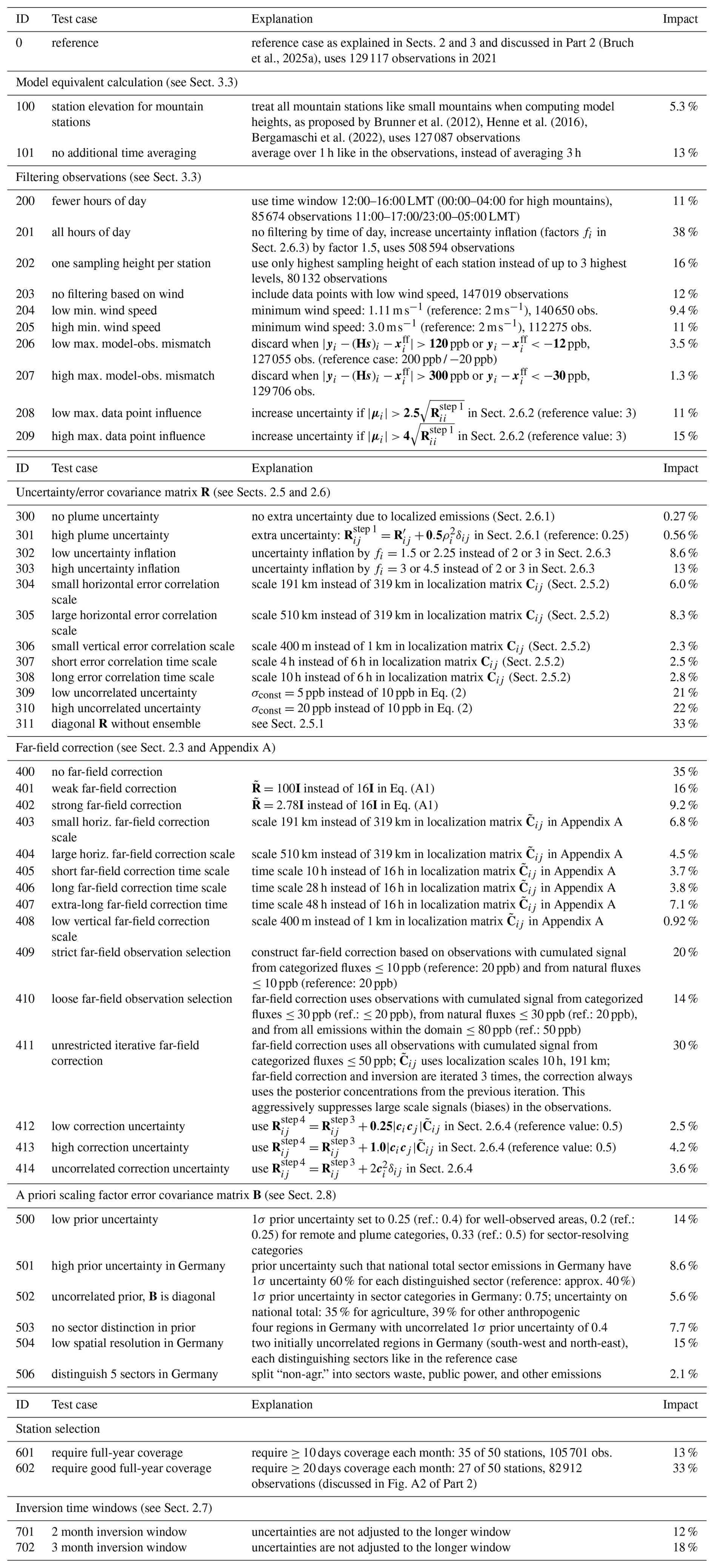
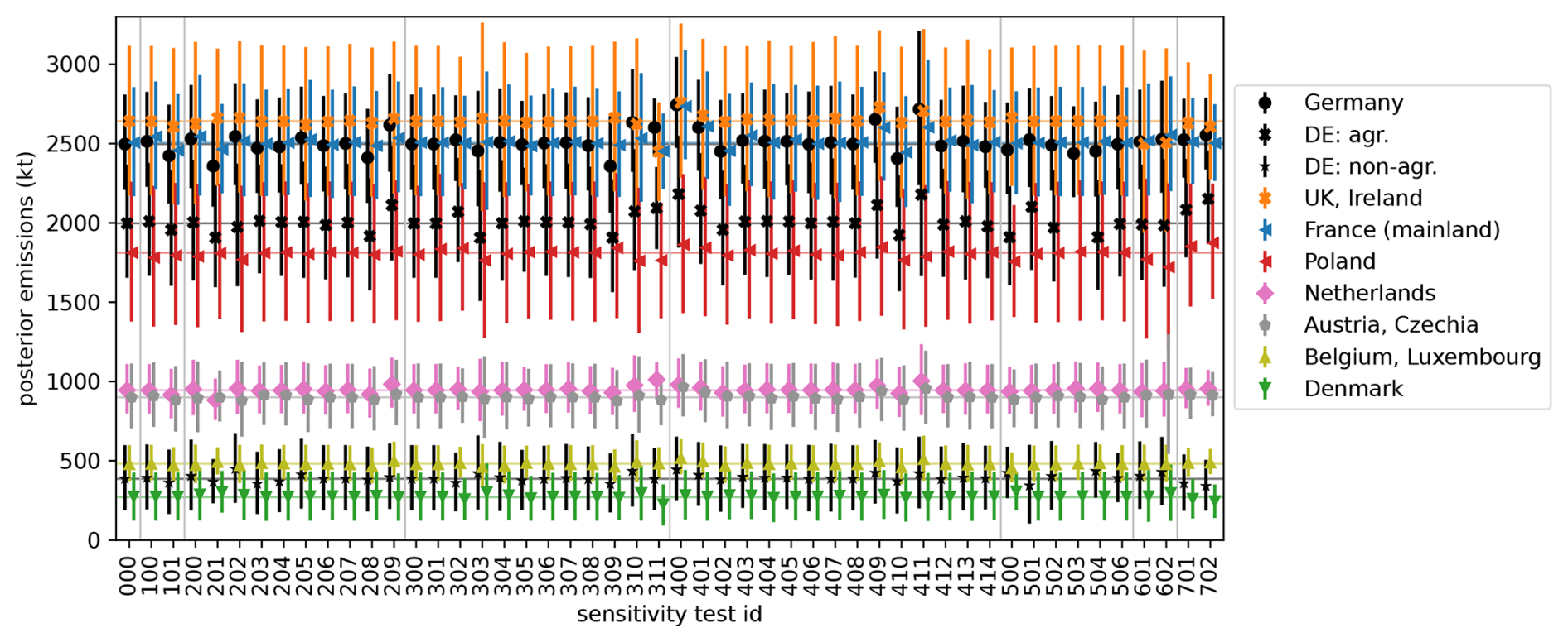
Figure E1 Posterior emissions and uncertainties of selected countries and German sectors for all sensitivity tests. Thin horizontal lines indicate the posterior of the reference case 0. Markers show the average of prior R and posterior R inversion. Vertical lines show uncertainties (95 % confidence intervals) and cover the uncertainty range of prior R and posterior R inversion. The individual tests are listed in Table E1. For all test cases, the emission estimates for the shown countries remain within the uncertainty range of the reference case.