Intercomparison of global ground-level ozone datasets for health-relevant metrics

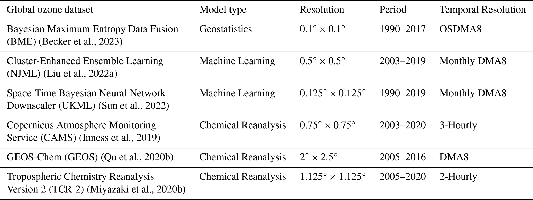
Ground-level ozone is a significant air pollutant that detrimentally affects human health and agriculture. Global ground-level ozone concentrations have been estimated using chemical reanalyses, geostatistical methods, and machine learning, but these datasets have not been compared systematically. We compare six global ground-level ozone datasets (three chemical reanalyses, two machine learning, one geostatistics) relative to observations and against one another, for the ozone season daily maximum 8 h average mixing ratio, for 2006 to 2016. Comparing with global ground-level observations, most datasets overestimate ozone, particularly at lower observed concentrations. In 2016, across all stations, grid-to-grid R² ranges from 0.50 to 0.75 and RMSE 4.25 to 12.22 ppb. Agreement with observed distributions is reduced at ozone concentrations above 50 ppb. Results show significant differences among datasets in global average ozone, as large as 5–10 ppb, multi-year trends, and regional distributions. For example, in Europe, the two chemical reanalyses show an increasing trend while other datasets show no increase. Among the six datasets, the share of population exposed to over 50 ppb varies from 61 % [28 %, 94 %] to 99 % [62 %, 100 %] in East Asia, 17 % [4 %, 72 %] to 88 % [53 %, 99 %] in North America, and 9 % [0 %, 58 %] to 76 % [22 %, 96 %] in Europe (2006–2016 average). Although sharing some of the same input data, we found important differences, likely from variations in approaches, resolution, and other input data, highlighting the importance of continued research on global ozone distributions. These discrepancies are large enough to impact assessments of health impacts and other applications.

1 Introduction

Tropospheric ozone is a secondary pollutant that significantly impacts human health, plant life, and the climate system. Past studies have shown that ozone exposure can cause health effects ranging from mild subclinical symptoms to mortality (Balmes, 2022). The Global Burden of Disease 2021 (GBD) study estimated that ground-level ozone contributed to approximately 490 000 (95 % UI: 107 000–837 000) global deaths in 2021, representing 0.72 % (95 % UI: 0.16 %–1.18 %) of all deaths that year (Brauer et al., 2024). Ozone exposure is harmful not only to humans but also to plants. Ozone can enter plants through their stomata and cause oxidative damage, which reduces the global yields of major crops such as soybean, wheat, rice, and maize (Ainsworth, 2017; Mills et al., 2018a). Ozone is also an important greenhouse gas, ranking third behind carbon dioxide and methane in its contribution to anthropogenic climate change (Masson-Delmotte et al., 2021). Gaudel et al. find that since the mid-1990s, tropospheric ozone above the surface has increased across all 11 study regions in the Northern Hemisphere that they defined and analyzed (Western North America, Eastern North America, Southeast North America, Northern South America, Northeast China/Korea, Persian Gulf, India, Southeast Asia, Malaysia/Indonesia, Europe, Gulf of Guinea) (Gaudel et al., 2020). In the United States, although extreme ground-level ozone concentrations have declined, winter ground-level ozone concentrations have increased in the Southwest and Midwest regions since 1990s (Chang et al., 2025). Using one global ozone dataset, from data fusion of ground observations and chemical model outputs, it is estimated that in 2017 21 % of the global population was exposed to ozone concentrations above 65 ppb, and 96 % lived in areas where concentrations exceeded the WHO guideline (30 ppb for annual metric) (Becker et al., 2023; DeLang et al., 2021). Despite existing assessments, substantial uncertainties remain due to observational gaps, especially in remote and developing regions. The lack of knowledge of the ground-level ozone distribution in these regions limits our ability to accurately assess ozone impacts on human health and crops.

The Tropospheric Ozone Assessment Report (TOAR) aggregates ozone observations from thousands of monitoring stations worldwide, forming the most extensive ground-level ozone monitoring data compilation to date (Schultz et al., 2017). Using the TOAR dataset, researchers have analyzed the global distribution, trends, and impacts of surface level ozone (Gaudel et al., 2018). Currently, the second phase of the Tropospheric Ozone Assessment Report (TOAR-II) aims to include additional ground-based stations, especially new networks in China and India. However, despite significant progress, there remain large regions with limited ground-based monitoring, and a gap in understanding ground-level ozone variations over time and space. To bridge gaps in regions lacking ozone monitors, various methods, including chemical reanalysis based long-term data assimilation, machine learning, and geostatistical methods have been employed. Chemical reanalysis is an approach that integrates observations from various sources including satellites using data assimilation and chemical transport models (CTMs) to reconstruct historical atmospheric chemical composition and understand long-term changes and trends in air quality and climate forcing (Miyazaki et al., 2020b). Tropospheric ozone records have been provided in recent chemical reanalyses including the Tropospheric Chemistry Reanalysis Version 2 (TCR-2; Miyazaki et al., 2020b), the Copernicus Atmosphere Monitoring Service (CAMS; Inness et al., 2019), and data assimilation using the GEOS-Chem adjoint model (GEOS-Chem; Qu et al., 2020b). In addition, two machine learning estimates of global ground-level ozone have been produced to date: one using a space-time Bayesian neural network trained on TOAR observations and CMIP6 simulations (Sun et al., 2022), and another with a cluster-enhanced ensemble learning method that utilizes various data sources (Liu et al., 2022a). Finally, geostatistical methods were applied by DeLang et al. who used Bayesian Maximum Entropy (BME) to estimate ozone through a data fusion of TOAR observations and output from multiple CTMs (DeLang et al., 2021). This approach was further enhanced by incorporating the Regionalized Air Quality Model Performance (RAMP) framework to correct model biases (Becker et al., 2023). These estimates of global ozone distributions and trends have supported analyses of health impacts. For example, ozone estimates of DeLang et al. (2021) were used in both the GBD 2021 study (Murray et al., 2020), and in a study of ozone health effects in urban areas globally (Malashock et al., 2022). However, there remains a lack of knowledge regarding the consistency of ground-level ozone estimates, distributions, and long-term trends across these global ozone mapping products.

Inconsistencies in these datasets could significantly impact public health research, especially in assessing the risks of ozone-related health impacts, and may impede the development of effective environmental policies and ozone management strategies (Post et al., 2012). Although each dataset incorporates a considerable amount of observational information and model simulations through various methodologies, each inherently incorporates biases from these input data sources during the fusion processes. While satellite measurements of precursor species can be used to constrain surface and lower tropospheric ozone in chemical reanalysis (Miyazaki et al., 2012), the performance of chemical reanalysis surface ozone is limited in part by the low sensitivities of satellite ozone measurements near the surface, as well as model simulation errors. Data fusion methods integrate outputs from multiple models with inherent biases, potentially propagating these biases to the final estimates (DeLang et al., 2021). Furthermore, machine learning methods trained on observation data may yield inaccuracies in rural and remote areas due to the uneven distribution of ground-level ozone monitoring stations (Liu et al., 2022a; Betancourt et al., 2022). Therefore, conducting comparisons and evaluations of various types of ground-level ozone mapping products is essential to understand the inconsistencies and biases in these datasets, ultimately benefiting global health studies.

This study aims to compare ground-level ozone concentrations estimated by six datasets, and to evaluate their accuracy over the 2006–2016 period, with a particular emphasis on their capacity to represent long-term ozone trends across different regions. The comparison and evaluation include three chemical reanalysis datasets, two machine-learning datasets, and one geostatistical dataset. The period 2006–2016 is chosen as the period over which the six datasets all produce ozone estimates. The ozone seasonal daily maximum 8 h average mixing ratio (OSDMA8) was selected as the health-relevant metric for annual ozone evaluation (Turner et al., 2016). Our study specifically utilizes the OSDMA8 metric because we focus on evaluating long-term ozone exposure, an aspect not comprehensively compared previously among global ozone mapping products. We employed a comprehensive set of indicators to assess the congruence between these datasets, globally and regionally, including for long-term population weighted ozone outdoor exposure. Relative to the latest TOAR-II observational dataset, this study also examines the six datasets' ability to estimate ground-level ozone concentrations across various regions for the years 2006–2016. This research endeavors to characterize differences among ground-level ozone datasets, including discrepancies in ozone estimates, distributions, and trends, that could hinder evaluation of ozone's effects on health and agriculture, as well as impede the formulation of effective environmental policies. Although the primary focus of this study is on health impacts, the results are also largely applicable to agricultural and ecosystem impacts.

2 Data

As shown in Table 1, this study compares and evaluates ground-level ozone estimates from six global ozone mapping products in three categories. We utilized ozone seasonal daily maximum 8 h average mixing ratio (OSDMA8) as the yearly ozone metric across all datasets. OSDMA8 is defined here as the maximum of the six-month running monthly mean daily maximum 8 h ozone (DMA8) from January of the current year wrapping to March of the following year (DeLang et al., 2021). OSDMA8 is GBD's ozone metric for quantifying health effect from long-term ozone exposure (Brauer et al., 2024), and it is the metric used in the World Health Organization's air quality guidelines, with values of 30 ppb for the guideline and 50 ppb for the interim target (World-Health-Organization, 2021). All observations and model estimates are converted to OSDMA8 using the same algorithm. Details on the input data used to construct each dataset are available in the Supplement.

Table 1 Overview of six global ozone mapping products.

2.1 Geostatistical ozone dataset

The BME dataset uses geostatistical methods to provide high-resolution global ground-level ozone estimates. First, M³Fusion (Measurement and Multi-Model Fusion) is a statistical method developed to improve estimates of global surface ozone distributions by integrating observational data from TOAR and outputs from multiple chemistry models. Specifically, the method assigns weights to multiple global atmospheric chemistry models based on their regional accuracy compared to observed ozone values (Chang et al., 2019), creating a composite of multiple global atmospheric chemistry models by weights. The details of input data can be found in Table S1 in the Supplement. Then BME data fusion integrates this multi-model composite with observations in space and time, and finally BME estimates are refined from 0.5° × 0.5° to 0.1° × 0.1° (DeLang et al., 2021). The observations are from TOAR-I for 1990 to 2017, complemented by data from the Chinese National Environmental Monitoring Center (CNEMC) for 2013 to 2017. The latest version of this dataset employs RAMP for bias correction of M³Fusion inputs (Becker et al., 2023). The BME ozone estimates are more accurate than the average outputs from multiple models, achieving an R² of 0.63 at 0.1° × 0.1° resolution, as evaluated against observations through cross-validation (DeLang et al., 2021). Furthermore, incorporating RAMP into the BME process significantly improves R² by 0.15, especially in areas far from monitoring stations, as demonstrated through checkerboard cross-validation (Becker et al., 2023).

2.2 Machine learning ozone datasets

We utilized two machine learning global ground-level ozone datasets from the University of Cambridge, and Nanjing University. The University of Cambridge's machine learning (UKML) dataset was developed using a space-time Bayesian neural network, fusing various data sources including historical observations, CMIP6 multi-model simulations (AerChemMIP historical simulations and ScenarioMIP projections), population distributions, land cover properties, and emission inventories (Sun et al., 2022) (input data summarized in Table S2). The UKML model categorized TOAR-I monthly ozone observations from 1990 to 2014 into urban and rural areas, and used these as labels for supervised learning. This model generates monthly global gridded ozone estimates from 1990 to 2019, downscaled to a 0.125° × 0.125° spatial resolution. It exhibited great performance in predicting urban and rural surface ozone concentrations, with R² values ranging from 0.89 to 0.97 and RMSE values between 1.97 and 3.42 ppb (Sun et al., 2022).

Nanjing University's machine learning (NJML) dataset was created using a cluster-enhanced ensemble machine learning method. This dataset integrates various data sources, including satellite observations, atmospheric reanalysis, land cover properties, emission inventories and meteorological features (Liu et al., 2022a). The main input data for NJML include meteorological parameters from ERA5, atmospheric chemistry from the CAMS chemical reanalysis, aerosol concentrations from MERRA-2, satellite observations from OMI/Aura, and emissions data from CEDS, spanning 2003-2019 with varying spatial resolutions (input data summarized in Table S3). It utilizes the monthly mean of daily maximum 8 h average (DMA8) data from TOAR-I and CNEMC observations from 2003–2019 as training data. The NJML dataset produces monthly global gridded ozone estimates from 2003 to 2019 with a 0.5° × 0.5° spatial resolution. The model demonstrates robust performance in both spatial and temporal predictions of ground-level ozone, with R² values of 0.909 and 0.925, respectively (Liu et al., 2022a).

2.3 Chemical reanalysis products

We utilized surface ozone analysis fields from three chemical reanalysis products: the Tropospheric Chemistry Reanalysis Version 2 (TCR-2; Miyazaki et al., 2020b), the Copernicus Atmosphere Monitoring Service reanalysis (CAMS; Inness et al., 2019), and the GEOS-Chem reanalysis (GEOS; Qu et al., 2020b). Different from the machine learning and geostatistical ozone datasets, the chemical reanalysis products utilized satellite observations of atmospheric composition to produce three-dimensional profiles of atmospheric composition. In situ surface observations were not included in the global chemical reanalysis data assimilation. Because of the lack of direct observational constraints, challenges remain in estimating surface ozone in the current reanalysis products (Huijnen et al., 2020). Detailed comparisons of these reanalyses for ozone over the entire troposphere at finer timescales have been conducted by the TOAR-II chemical reanalysis working group (Sekiya et al., 2025; Jones et al., 2024; Miyazaki et al., 2025), but without a focus on the ground level and long-term metric as analyzed here.

TCR-2 was generated by assimilating multiple satellite observations into the MIROC-Chem model, that was developed as a part of the multi-model multi-constituent data assimilation (Miyazaki et al., 2020a). The meteorological fields were nudged to the European Centre for Medium-Range Weather Forecasts (ECMWF) Interim Reanalysis meteorology. The data assimilation employed is an ensemble Kalman filter technique, which was used to effectively correct the emissions and concentrations of various chemical species (Miyazaki et al., 2020b). The assimilated data include ozone, CO, NO₂, HNO₃ and SO₂ from satellite instruments such as OMI, MLS, GOME-2, SCIAMACHY and MOPITT over the period from 2005 to 2021 (input satellite data summarized in Table S4). TCR-2 provides 2-hourly global ozone profiles at a 1.1° × 1.1° spatial resolution, with the regional mean ozone bias against global ozonesonde measurements ranging from −0.4 to 4.2 ppb in the lower troposphere (850–500 hPa) (Miyazaki et al., 2020b).

CAMS, operated by the European Centre for Medium-Range Weather Forecasts (ECMWF) on behalf of the European Commission, provides the global reanalysis dataset on atmospheric composition developed by ECMWF. The main inputs for the CAMS ECMWF Atmospheric Composition Reanalysis 4 (EAC4) chemical reanalysis are retrievals of CO, ozone, NO₂ and aerosol optical depth (AOD) from multiple satellite instruments including MLS, OMI, GOME-2, SCIAMACHY, MIPAS, SBUV/2 and MOPITT, covering various periods ranging from 2003 (input satellite data summarized in Table S5). CAMS employed the four-dimensional variational data assimilation (4D-Var) method to integrate the satellite measurements under ECMWF's Integrated Forecasting System (IFS) CB05 model (Inness et al., 2019). It provides 3-hourly global profiles of ozone and other species at a 0.75° × 0.75° spatial resolution. While CAMS generally improves over previous analyses, challenges and biases remain, particularly at high latitudes and in accurately capturing seasonal variations (Inness et al., 2019).

The GEOS-Chem dataset is developed through 4D-Var data assimilation of NO₂ column densities using the GEOS-Chem adjoint model that includes updates in stratospheric and halogen chemistry (Henze et al., 2007). The GEOS-Chem model is driven by the Modern-Era Retrospective analysis for Research and Applications, Version 2 (MERRA-2) meteorological fields from the NASA Global Modeling and Assimilation Office (GMAO). Prior anthropogenic emissions of NO_x, SO₂, NH₃, CO, NMVOCs (non-methane volatile organic compounds), and primary aerosols were obtained from the HTAP 2010 inventory version 2 (Janssens-Maenhout et al., 2015) (input data summarized in Table S6). Operating at a 2° × 2.5° resolution, the assimilation estimates global ozone more accurately than the forward model from 2006 to 2016 by deriving emissions of NO₂ through inverse modelling. The GEOS-Chem dataset exhibits a small bias across all ozone metrics, and among metrics it has the best spatial consistency for DMA8 (R² = 0.88) (Qu et al., 2020b). However, the model has limitations in accurately capturing regional variations and seasonal trends in ozone concentrations.

2.4 Ground-level ozone observations

For the evaluation in this project, we utilized both urban and non-urban ground-level ozone observations for the yearly OSDMA8 metric from the updated TOAR-II dataset, covering 2006 to 2016 (Schröder et al., 2021). This dataset represents the most extensive collection of tropospheric ozone measurements available globally. Compared to TOAR-I (Schultz et al., 2017), TOAR-II incorporates an expanded dataset of ozone observations, notably including monitoring data from approximately 1400 stations across China for the years 2015 to 2016 that are included in TOAR-II (https://toar-data.fz-juelich.de/gui/v2/dashboard/, last access: 15 November 2024). We require that at least 75 % of the days in a month must have valid DMA8 values for that month to be included in the annual data calculations. The total number of observation sites used in our assessment varied from a minimum of 3715 in 2006 to a maximum of 7013 in 2016. Given that three ozone products in this study utilize the TOAR-I dataset for training or input, evaluations using the latest TOAR-II dataset for sites not included in TOAR-I can provide more objective results. Figure S1 illustrates the spatial distribution of TOAR-II monitoring stations in 2016. We use the TOAR-II database as it existed in May 2025. Because of possible errors in measurement units, we omit all data from France in 2014.

2.5 Population data

We analyzed ozone population exposures for each dataset using the globally gridded population data for the year 2019 from the Global Burden of Disease (GBD) 2019, which has a resolution of 0.1° × 0.1° (Lloyd et al., 2019). Since we use the same gridded population data for all years of the project, we focus on differences in exposure attributable to changes in ozone levels rather than changes in population. Therefore, population-weighted ozone over 2006 to 2016 can be biased even if the ozone data are unbiased.

3 Methodology

3.1 Evaluation with ground-level observation

Previous research created 1° × 1° grid-cell-averaged hourly ozone data from surface observations to evaluate global chemistry model performance over North America and Europe, which is suitable for analyzing extremes and validating seasonal and diel ozone cycles (Schnell and Prather, 2017; Schnell et al., 2015). We utilized OSDMA8 from TOAR-II observations covering 2006 to 2016 to evaluate the six datasets. During the evaluation process, we retained the original resolution of the six datasets (Table 1).

Considering that the six datasets have different resolutions and are designed for different applications, we adopted a dual evaluation strategy to provide a comprehensive assessment of their performance. The first method is a grid-to-grid evaluation. Similar to the approach of Schnell et al. (2015), we re-gridded TOAR-II observations to a 0.1° × 0.1° resolution by an inverse distance weighted method and then aggregated them to match the native resolution of each of the six datasets. In this approach, the sample size for each evaluation varies reflecting the varying resolution of the datasets; for 2016, BME had 173 718 grid cell pairs, NJML had 7099, UKML had 162 419, CAMS had 4614, GEOS-Chem had 782, and TCR-2 had 2195. We also adopted the grid-to-grid evaluation method for regional evaluations, as it provides better spatial representativeness over large areas. To quantify the uncertainty of the six datasets' estimates, we determined the lower and upper bounds (95 % confidence interval), derived from the grid-to-grid regression analysis performed between the TOAR-II observations and each of the six datasets at their native resolutions.

The second method is a standard grid-to-point evaluation. This approach ensures a consistent sample size across all datasets by comparing each dataset's estimate at the grid cell containing an observation location. For grid cells containing a TOAR-II site but no valid estimate (NA value), we used the nearest valid estimate instead. This method captures a penalty for missing data and coarse resolution, only BME, NJML, and UKML had a small number of missing estimates at TOAR-II locations. The grid-to-point method was used to evaluate model bias, as it ensures a consistent sample size across all datasets when performing evaluations on different quantiles of the TOAR-II observations. For both methods, we assessed the performance of each dataset using the coefficient of determination (R²) between ozone estimates and observations, and root mean square error (RMSE) as the primary metrics. We selected the 50 ppb as the threshold for high ozone concentration because it corresponds to the long-term air quality interim target of WHO.

3.2 Pairwise spatial similarity comparison

Before comparing concentration estimates between datasets, we converted all ozone estimates from each dataset to OSDMA8, ensuring only one ozone estimate value per year for each grid cell (see the original temporal resolution in Table 1). The OSDMA8 metric is used for long-term ozone exposure given its utility and wide acceptance in health impact studies, despite the inherent loss of shorter temporal dynamics. We employed two quantitative metrics to classify how the datasets relate with one another: the Pearson correlation coefficient (R) and the root mean square difference (RMSD). The pairwise correlation R indicates the similarity in geographical distribution of ozone concentrations, and the RMSD quantifies the difference in ozone estimates between datasets. A higher R value suggests greater similarity in the spatial pattern between two datasets and a smaller RMSD indicates a less significant discrepancy in ozone concentration estimates between two datasets. We then group the six datasets, adopting a method that maximizes the difference between the correlation R within and outside the groups. The idea of this grouping is to distinguish the spatial similarity between the datasets, which is based on the pairwise correlation. For each grouping combination, 4 variables are computed: the sum of pairwise correlations within groups (C_i), the sum of pairwise correlations outside the groups (C_o), the number of dataset pairs within groups (N_i), and the number of dataset pairs outside the groups (N_o). The objective is to ascertain the grouping combination that maximizes the difference between $C_{\mathrm{i}}/N_{\mathrm{i}}$ and $C_{\mathrm{o}}/N_{\mathrm{o}}$. More details of the calculation can be found in Sect. S1.

3.3 Long-term exposure comparison

Subsequently, we re-gridded all datasets and TOAR-II observations to 0.1° × 0.1° resolution to facilitate comparison at the same spatial scale. During re-gridding, we ensure that the average value of the finer grid cells matches that of the original coarse grid cell; for example, if a grid cell has a value of 30 ppb, then after re-gridding to finer grid cells, the average value of these grid cells will still be 30 ppb. Data over the ocean were excluded, retaining only land and populated islands for analysis. We calculated the yearly ozone trend using 50 % quantile regression for each dataset using both population-weighted and area-weighted approaches, with details of the calculation methods provided in Sect. S2. In this study, the trend is interpreted from the slope of the quantile regression, and confidence in the trend is determined by its p-value: p ≤ 0.01 is considered very high certainty; 0.01 < p ≤ 0.05, high certainty; 0.05 < p ≤ 0.1, medium certainty; 0.1 < p ≤ 0.33, low certainty; and p > 0.33, no evidence. We also regressed population-weighted mean ozone concentrations in different world regions of each dataset against the year to evaluate ozone long-term variations. For each grid cell we calculated the mean and standard deviation of the six OSDMA8 values obtained from each dataset to highlight regional differences and similarities. We also calculated the deviation from the ensemble mean for each dataset to assess geographic distribution variations.

Furthermore, we compared ozone exposure differences in various regions for each dataset to evaluate the potential for health impacts. Here we estimate exposure as the ambient concentration in 0.1° × 0.1° grid cells related to population at their residences, not including other factors that affect human exposure such as time-activity patterns. To quantify the uncertainty in our exposure analysis, we established lower and upper bounds for all population exposure and share of population estimates. The OSDMA8 95 % confidence interval (CI) for each dataset is determined through a grid-to-grid linear regression between each dataset and the re-gridded TOAR-II observations based on 0.1° × 0.1° grid cells. We use regional groupings defined by HTAP2 (Koffi et al., 2016), as detailed in the Table S7.

4 Evaluation against TOAR-II observations

4.1 Evaluation of ground-level ozone in 2016

We conducted regression and bias analyses for each dataset in comparison with TOAR-II observations for each year from 2006 to 2016. Figure 1a and c illustrates the scatterplot from the linear regression analysis of each dataset against the 7013 TOAR-II observations in 2016, accompanied by a density core that visualizes the data point distribution. The year 2016 is presented here because it has the highest number of TOAR-II observations from 2006 to 2016, and other years can be found in Figs. S2 and S3. For 2016, BME outperforms other datasets in both evaluation method, with the highest R² (0.75 for grid-to-grid, 0.63 for grid-to-point) and lowest RMSE (4.25 ppb for grid-to-grid, 5.28 ppb for grid-to-point), its density cores intersecting the y=x line. BME has an advantage in that its methods should nearly match the observed values for locations used as inputs to the data fusion. Consequently, we conduct another validation for TOAR-II sites not used as input for BME in 2016 (Fig. S4). After excluding all sites located at observation points previously used as BME input, using 3911 observations for validation, BME performs well compared to another datasets, though its R² decreases significantly to 0.65 for grid-to-grid and 0.53 for grid-to-point. In Fig. 1a, all three chemical reanalysis datasets exhibit a moderate R² ranging from 0.51 to 0.60 for grid-to-grid and 0.35 to 0.41 for grid-to-point, comparable to the performance of the machine learning datasets, which have R² values of 0.50 and 0.56 for grid-to-grid, 0.37 and 0.38 for grid-to-point. Among these five datasets, CAMS has the lowest RMSE (6.00 ppb for grid-to-grid and 7.59 ppb for grid to point), which is better than other chemistry reanalysis products but relatively low R² (0.51 for grid-to-grid and 0.35 for grid-to-point). Its density cores slightly below the y=x line suggests CAMS estimates are marginally lower than TOAR-II observations. GEOS-Chem and TCR-2 demonstrate adequate performance, albeit with higher RMSE values of 8.47 and 10.26 ppb for grid-to-grid, 10.27 and 13.23 ppb for grid-to-point, respectively. Their density cores positioned above the y=x line indicate that these models tend to produce higher estimates compared to the TOAR-II observations. NJML shows acceptable performance with higher R² (0.56 for grid-to-grid and 0.38 for grid-to-point) than CAMS and lower RMSE (6.37 ppb for grid-to-grid and 8.63 ppb for grid-to-point) than TCR-2. UKML exhibits the highest RMSE of 12.22 ppb for grid-to-grid and 13.49 ppb for grid-to-point, and its density cores region are above the y=x dashed line, indicating an overestimation. This is because the UKML algorithm emphasizes higher ozone pollution levels in rural and remote areas compared to adjacent urban districts, which consequently leads to an overestimation especially in population-weighted metrics (Sun et al., 2024).

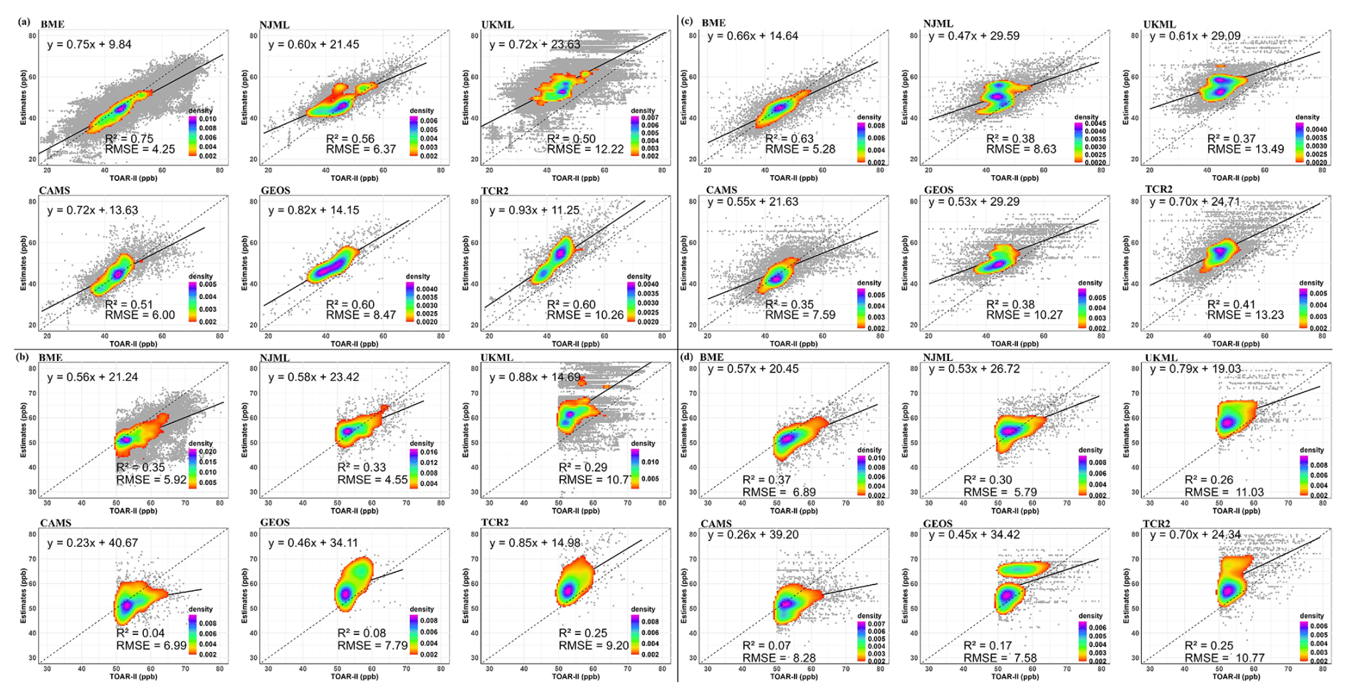
Figure 1 Performance evaluations of six datasets with TOAR-II observations in 2016 for OSDMA8. The observation-prediction evaluations are presented with densities estimated by a Gaussian kernel function. The coefficient of determination (R²) and root mean squared error (RMSE) are shown for four scenarios: (a) a grid-to-grid evaluation at the native resolution of each dataset using re-gridded TOAR-II observations, (b) a grid-to-grid evaluation, same as panel (a), but only for grid cells with observations above 50 ppb, (c) a grid-to-point evaluation using all TOAR-II sites, (d) a grid-to-point evaluation, same as panel (c), but only for sites with observations above 50 ppb. The dashed line marks where TOAR-II observations equal estimates (y=x line), and the solid black line represents the best-fit line. Performance evaluations for each year are shown in Figs. S7 and S8.

Figure 1b and d focuses only on TOAR-II grid cells or sites with OSDMA8 value above 50 ppb, showing that R² is reduced compared to the comparison of all ozone measurements (Fig. 1a and c) for all six datasets, suggesting overall weaker agreement between modeled and observed ozone distributions at higher concentrations. All six datasets show decreasing performance from BME, NJML, and UKML to TCR-2, GEOS-Chem, and CAMS, with R² of 0.35, 0.33, 0.29, 0.25, 0.08, and 0.04 for grid-to-grid; 0.37, 0.30, 0.26, 0.25, 0.17, and 0.07 for grid-to-point, respectively. However, the change of biases varies among datasets at higher concentrations. Specifically, overestimation is reduced in the UKML, NJML, GEOS-Chem, and TCR-2 datasets when observations exceed 50 ppb in both evaluation methods. Conversely, we observe increased underestimation in the BME and CAMS datasets at ozone levels above 50 ppb. This proportional bias is consistent with the linear regression slope, which is less than 1 for all six datasets in Fig. 1. Figure 2 shows the normalized mean bias for stratified concentration intervals in 2016, which provides insights into the average discrepancy between estimates and TOAR-II observations across ozone concentration ranges. All six datasets overestimate TOAR-II observations below the 40 % concentration interval. Only BME underestimates above the 40 % concentration level, CAMS underestimates above the 80 % concentration interval, and NJML underestimates above 90 % concentration interval, aligning with the density kernel presented in Fig. 1. BME demonstrates the smallest mean bias, particularly below the 50 % concentration level and CAMS shows the smallest mean bias in the 50 % to 90 % concentration interval. In the 90 % to 100 % concentration interval, NJML and GEOS-Chem have the smallest mean bias. In summary, BME and CAMS perform better overall in terms of normalized mean bias, with other models tending to overestimate ozone at almost all concentrations. Detailed plots of normalized mean bias for stratified concentration intervals for each year from 2006 to 2015 are shown in Fig. S5.

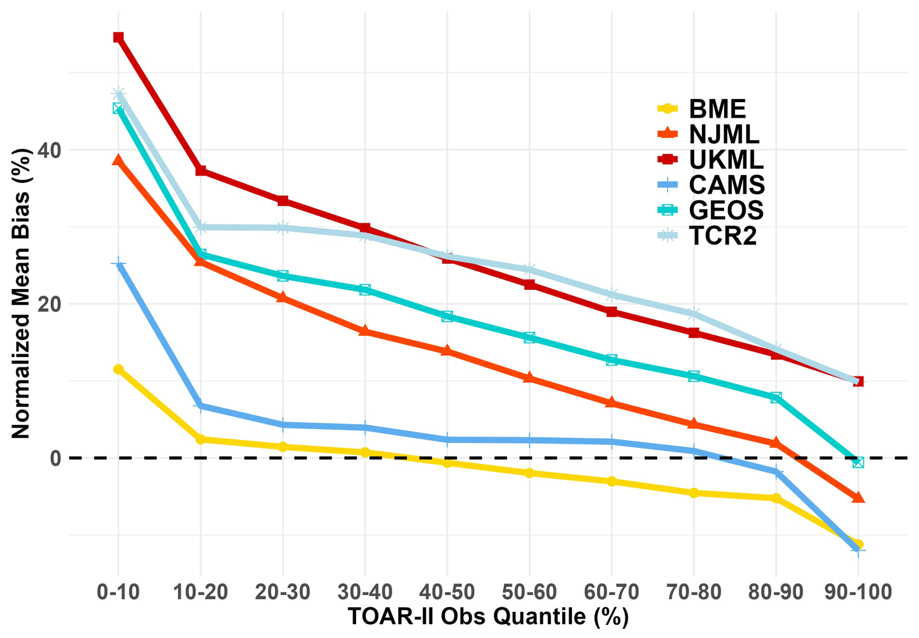
Figure 2 Normalized mean bias of six databases against TOAR-II observations (OSDMA8) at different quantiles in 2016, calculated based on the grid-to-point scenario. 0 %: 13.46 ppb; 10 %: 36.75 ppb; 20 %: 39.80 ppb; 30 %: 41.89 ppb; 40 %: 43.57 ppb; 50 %: 45.06 ppb; 60 %: 46.82 ppb; 70 %: 48.93 ppb; 80 %: 52.18 ppb; 90 %: 57.21 ppb; 100 %: 86.25 ppb. Normalized mean bias for each year against TOAR-II observations are shown in Fig. S5. Different quantiles of TOAR-II observations for other years are shown in Table S11.

4.2 Evaluation of ground-level ozone in different countries or regions

Figure 3 presents the distribution of population exposure calculated from six datasets and the gridded TOAR-II observations in three world regions with a high density of observations, for 2016. Here we calculate the population-weighted kernel density for population exposure to OSDMA8 concentrations, based on the 0.1° × 0.1° resolution for each region, only for grid cells where the re-gridded TOAR-II data have a value. Corresponding plots for other years (2006 to 2015) are shown in Fig. S6. Overall, the datasets are widely distributed, and the estimated exposure peaks vary. In East Asia (EAS), the population is exposed to high ozone concentrations. The concentration distribution is broad and has multiple peaks from TOAR-II observations, indicating a complex pollution environment, with a large population exposed to concentrations frequently exceeding 50 ppb, even 70 ppb. BME and NJML show a similar distribution as TOAR-II. Significant differences exist between UKML, CAMS and GEOS-Chem with the TOAR-II data for EAS. In Europe (EUR), exposure is concentrated between 40 and 50 ppb, indicating a more moderate and uniform exposure. The BME and CAMS have the best fit with the TOAR-II. NJML, UKML, GEOS-Chem, and TCR-2 show a peak at a higher ozone concentration range of 50–60 ppb. In North America (NAM), exposure peaks sharply in the 40 to 50 ppb range, which is slightly higher and more concentrated than in Europe. The NJML dataset agrees best with the shape of the TOAR-II distribution, and GEOS-Chem and BME capture the overall shape of the major exposure peaks well.

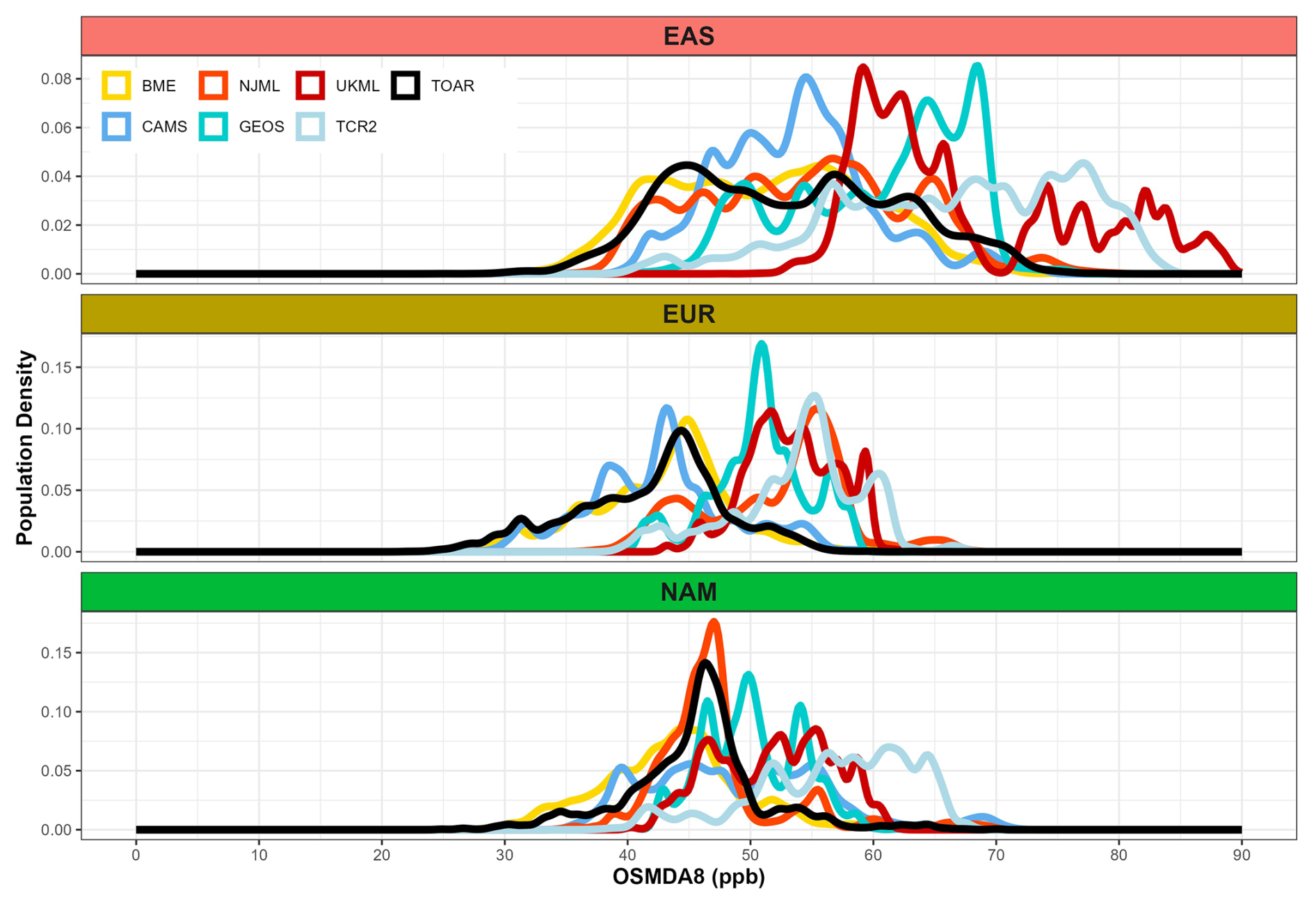
Figure 3 Population-weighted exposure distributions for OSDMA8 in 2016 in three regions: East Asia (EAS), Europe (EUR), and North America (NAM) (regions defined in Table S7). Each panel compares the distribution derived from the TOAR-II observations (black line) with estimates from six datasets (colored lines), calculating the population-weighted kernel density estimate, only for grid cells where TOAR-II measurements exist.

Table 2 Performance evaluation of six datasets for countries (and the EU) with the most monitors in 2016 against TOAR-II observations of OSDMA8 based on the gird-to-grid scenario. Number is the number of the TOAR-II monitor stations in each country. Density (per km²) is the density of the TOAR-II monitors in each country based on land area. Estimate is the average of the grid estimates for each dataset at the TOAR-II monitor locations in each country. Linear regression R² and root mean squared error (RMSE) against TOAR-II observations in each country are based on a grid-to-grid evaluation at each dataset's native resolution against re-gridded TOAR-II observations. The Lower and Upper Bound represent the 95 % confidence interval for the Estimate, calculated from the linear regression of each dataset against TOAR-II observations. Country names are United States of America (USA), China (CHN), Japan (JPN), South Korea (KOR), Canada (CAN). EU-27 includes Austria, Belgium, Bulgaria, Croatia, Cyprus, Czech Republic, Denmark, Estonia, Finland, France, Germany, Greece, Hungary, Ireland, Italy, Latvia, Lithuania, Luxembourg, Malta, Netherlands, Poland, Portugal, Romania, Slovakia, Slovenia, Spain, Sweden. Others is all other countries in TOAR-II apart from those listed. Performance evaluations for other years in these countries, are shown in Table S8.

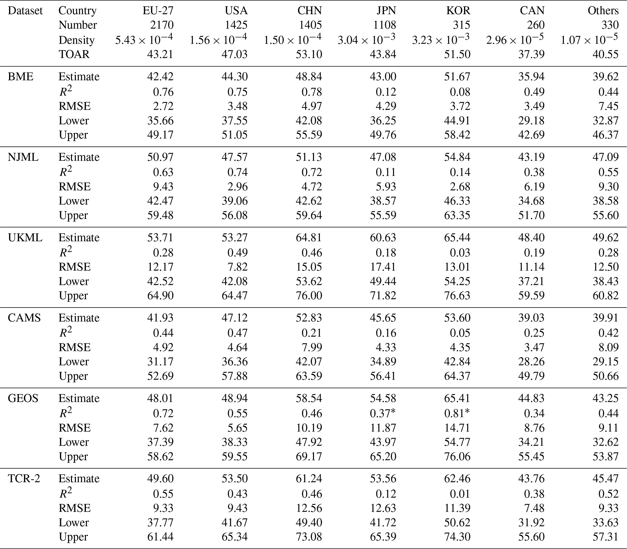
^∗ indicates the sample size of the comparison pair is less than 30.

Table 2 presents the validation results for different countries or regions using re-gridded TOAR-II observations at each dataset's native resolution in 2016, focusing on the countries with the highest number of sites. Here we use R² to assess the strength of the spatial correlation and RMSE to measure the bias across each country or region. The performance of each dataset varies by region, indicating that a dataset's overall performance does not guarantee its effectiveness in all regions. Reasonable R² and RMSE values are seen across all 6 datasets in the United States; BME leads with the highest R² (0.75) and lowest RMSE (3.48 ppb), and TCR-2 has the lowest R² (0.43) with highest RMSE (9.43 ppb). In Japan, BME leads with an RMSE of 4.29 ppb, followed by CAMS at 4.33 ppb, and UKML has the highest RMSE (17.41 ppb).

The datasets also perform poorly in South Korea, where GEOS-Chem has the highest RMSE (14.71 ppb) and NJML has the lowest RMSE (2.68 ppb). Although Japan and South Korea have a dense network of monitors, nearly all datasets show a weak correlation with observations, with R² below 0.2. Only the GEOS-Chem dataset has the highest R² value of 0.37 in Japan and 0.81 in South Korea, this result should be interpreted with caution, as the evaluation includes fewer than 30 grid-to-grid pairs. The performance of datasets within China exhibits significant variability, where BME and NJML demonstrate relatively good performance, and CAMS exhibits poor performance for R², while for RMSE, CAMS performs better than GEOS-Chem, TCR-2 and UKML. For other countries, which serve as a test of model performance in areas with sparse observations, nearly all datasets exhibit better R² values than in South Korea and Japan, with TCR-2 and NJML demonstrating particularly better performance than others. Overall, BME demonstrates strong performance in most countries, particularly in the United States, where it achieves the highest R² and the lowest RMSE, suggesting both strong spatial correlation with TOAR-II observations and high accuracy. NJML exhibits mixed performance, with relatively high R² values indicating good correlation in the United States and China, but it falls short in EU-27 with high RMSE. UKML presents consistently high RMSE values across countries suggesting high bias. CAMS displays variable performance with low R² values in China, indicating a lack of spatial correlation, yet its RMSE values are relatively small across all regions when compared to other chemical reanalysis datasets. Compared to CAMS, GEOS-Chem and TCR-2 exhibit better spatial correlations in Europe, the United States, China, and Canada. However, TCR-2 also presents high RMSE values across all regions. Five datasets except GEOS-Chem exhibit lower spatial correlation compared to TOAR-II observations in countries with high monitoring density, such as Japan and South Korea, than in countries with lower monitoring densities. NJML, UKML, GEOS-Chem and TCR-2 show overestimates compared to the TOAR observations in every country in the Table 2. Extending the analysis to the period from 2006 to 2016 (see tables in Table S8), the percentage of underestimates from 6 datasets compared to TOAR observations in all countries is below 20 %.

4.3 Evaluation of ground-level ozone across different years

Figure 4 presents time series plots of R² and RMSE from grid-to-grid and grid-to-point evaluations of each dataset against TOAR-II observations from 2006 to 2016. It is important to note that the years 2015 and 2016 include observations from China. In Fig. 4a and c BME consistently shows the largest R², indicating its robust performance near the monitor locations due to the utilization of observational data as input and the effective exploitation of spatiotemporal autocorrelation among stations. Apart from BME, for both evaluation scenarios NJML outperforms other datasets in R² from 2010 to 2014, and TCR-2 leads in 2007 and 2016. In grid-to-point evaluation, five datasets, excluding NJML, demonstrate a drop in R² in 2010, and all datasets show an increase in R² from 2015 to 2016. In grid-to-grid evaluation, GEOS-Chem shows an overall better performance in R² than CAMS, TCR-2 and UKML. For both scenarios, BME maintains the lowest RMSE throughout the period, indicating the most accurate predictions. CAMS also performs well in terms of RMSE. From 2006 to 2013, GEOS-Chem consistently has lower RMSE than both TCR-2 and UKML. Meanwhile, NJML exhibits a decreasing RMSE from 2006 to 2016. The clear differences in time series of RMSE correspond with the yearly mean trends in Fig. 5. Datasets with lower ozone values, BME and CAMS, also exhibit lower RMSE, whereas those with higher estimates, specifically TCR-2 and UKML, have higher RMSE. From 2006 to 2016, the performance rankings derived from R² values varied significantly between the two evaluation scenarios, whereas the RMSE based rankings were nearly consistent.

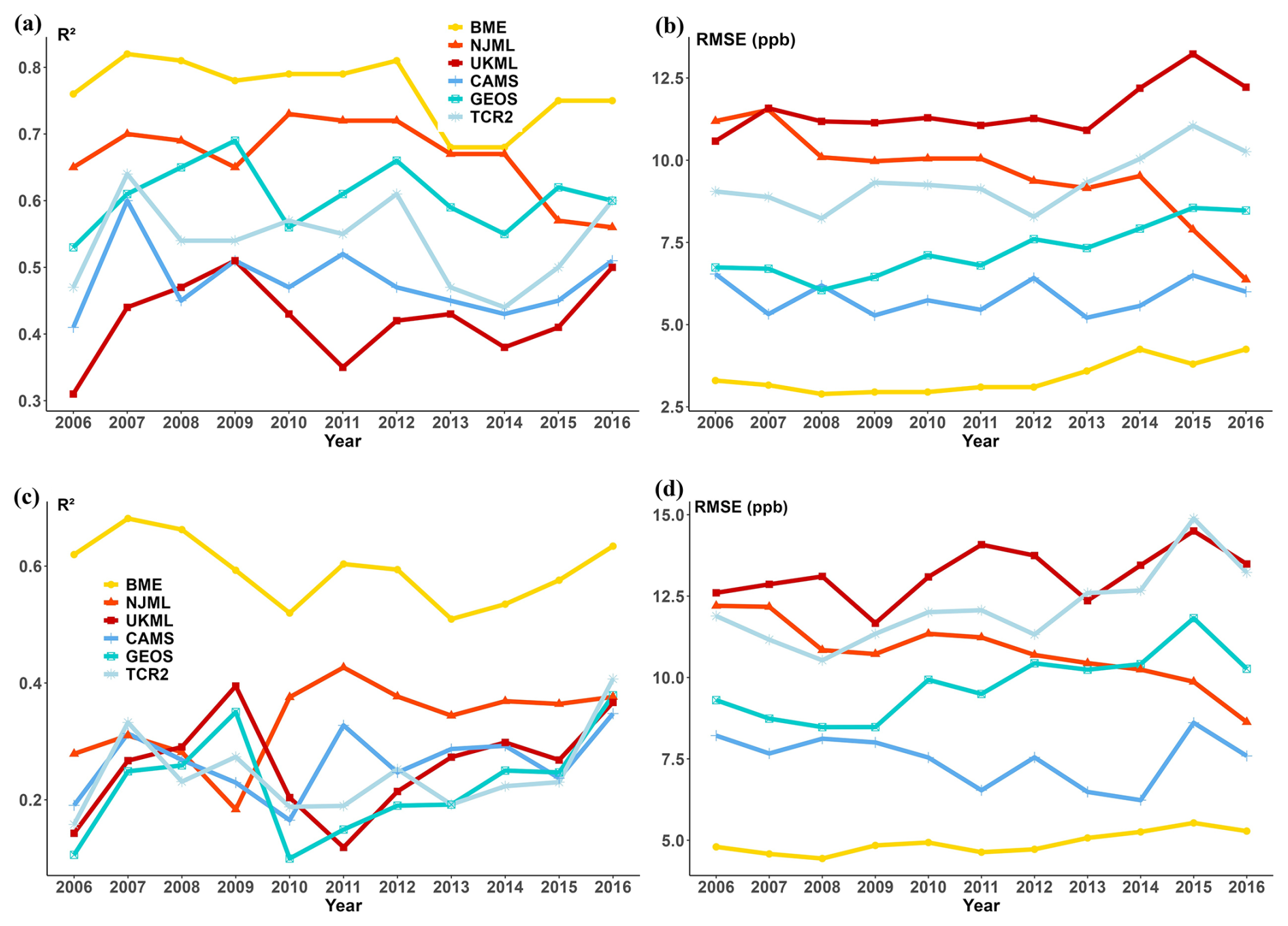
Figure 4 (a) Time series of determination (R²) between each dataset and TOAR-II observations of OSDMA8 from 2006 to 2016 based on grid-to-grid evaluation at the native resolution of each dataset using re-gridded TOAR-II observations. (b) Time series of root mean squared error (RMSE) between each dataset and TOAR-II from 2006 to 2016 based on grid-to-grid evaluation. (c) Time series of determination (R²) between each dataset and TOAR-II observations of OSDMA8 from 2006 to 2016 based on grid-to-point evaluation using all TOAR-II sites. (d) Time series of root mean squared error (RMSE) between each dataset and TOAR-II from 2006 to 2016 based on grid-to-point evaluation.

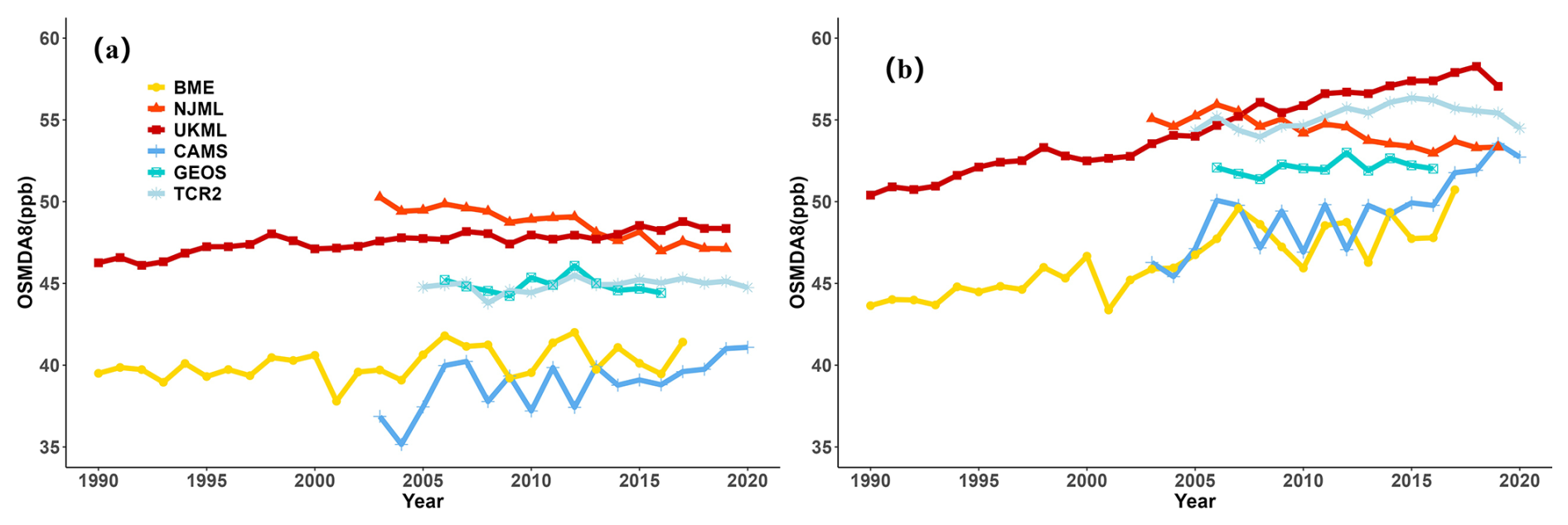
Figure 5 Yearly trends of ground-level ozone for six datasets, shown for (a) the area weighted global mean ozone over land, and (b) population weighted global mean ozone, where ozone is expressed as OSDMA8. Yearly trends for individual world regions are shown in Figs. S2 and S3. Mann-Kendall trend test for population weighted global mean over the full time series for each dataset: BME 0.688 ppb yr⁻¹ trend with p-value < 0.0001, NJML −0.691 ppb yr⁻¹ with p-value 0.0001, UKML 0.913 ppb yr⁻¹ with p-value < 0.0001, CAMS 0.569 ppb yr⁻¹ with p-value 0.0011, GEOS-Chem 0.164 ppb yr⁻¹ with p-value 0.5334, TCR-2 0.4 ppb yr⁻¹ with p-value 0.0343.

5 Comparison between ozone mapping products

5.1 Temporal trends

Both the area-weighted and population-weighted mean trends of global OSDMA8 reveal substantial differences among global ozone mapping datasets (Fig. 5). Notably, BME and CAMS have lower ozone values than other datasets, for both metrics, while UKML and NJML have higher ozone estimates, with differences between these datasets exceeding 5 ppb. The higher values in GEOS-Chem and TCR-2 may be attributed to the remaining high bias in the forecast models, which is commonly found in CTMs (Travis and Jacob, 2019). The population-weighted mean is higher than the area-weighted mean, by 5–10 ppb across all datasets, and for UKML and BME, the disparity between population-weighted and area-weighted ozone concentrations appears to widen over time. The faster increase in the population-weighted mean compared to the area-weighted mean appears to be driven by rising ozone levels in highly populated regions. In Table 3, focusing on 2006 to 2016, we find that NJML was the only dataset to exhibit a downward trend with very high certainty for both area- and population-weighted mean ozone concentrations. In contrast, TCR-2 and UKML only show increasing trends in population-weighted mean ozone during this period with very high certainty. However, while the BME dataset shows a negative slope for the area-weighted mean, this downward trend has only low certainty; for the population-weighted mean, there is no evidence of a decreasing trend. Figure 6 illustrates regional ozone changes per decade, weighted by population, across different regions in each dataset over 2006 to 2016. NJML, despite its overall decreasing trend in Table 3, does not uniformly show declines across all regions. The decrease in NJML is predominantly in North America, notably over 8 ppb per decade in the US and Canada, while Sub Saharan Africa and South America exhibit increases. BME and UKML, with the longest duration, both display decreasing trends in North America, and Europe, and increases in Southeast Asia and Middle East. Both datasets indicate greater decreases in North America than in Europe and more significant increases in the Middle East than in Southeast Asia. However, BME shows a downward trend in East Asia, while UKML exhibits the reverse. CAMS and TCR-2's trends in Fig. 6 are less distinct, except for the decrease in North America and the increase in East Asia, mirroring those of GEOS-Chem, which exhibits the smallest decadal ozone change, likely due to not directly assimilating ozone from satellite observations. From Table S9, we observe that some regions exhibit a clearer trend from 2006 to 2016, with very high certainty across six datasets. In East Asia, BME and NJML observe decreasing trends, whereas the other 4 datasets display increasing trends. In North America, all datasets display a downward trend, and in Europe, BME, NJML, UKML and TCR-2 show a decline, contrasting with increases in CAMS and GEOS-chem. Recent analyses using TOAR observations indicate that from 2006 to 2016, most sites in North America experienced decreasing ozone, while many sites in East Asia exhibited significant positive trends (Chang et al., 2025; Fleming et al., 2018; Chang et al., 2017). These observed trends in North America, Europe and East Asia seem to agree best with the trends estimated by BME and UKML. Detailed plots of population weighted and area weighted trends for each dataset in each region are shown in Figs. S7 and S8.

Table 3 Yearly trends of area-weighted, and population-weighted global mean of ground-level ozone for six datasets with 95 % confidence intervals (LowerCI and UpperCI) and p-values from 2006 to 2016.

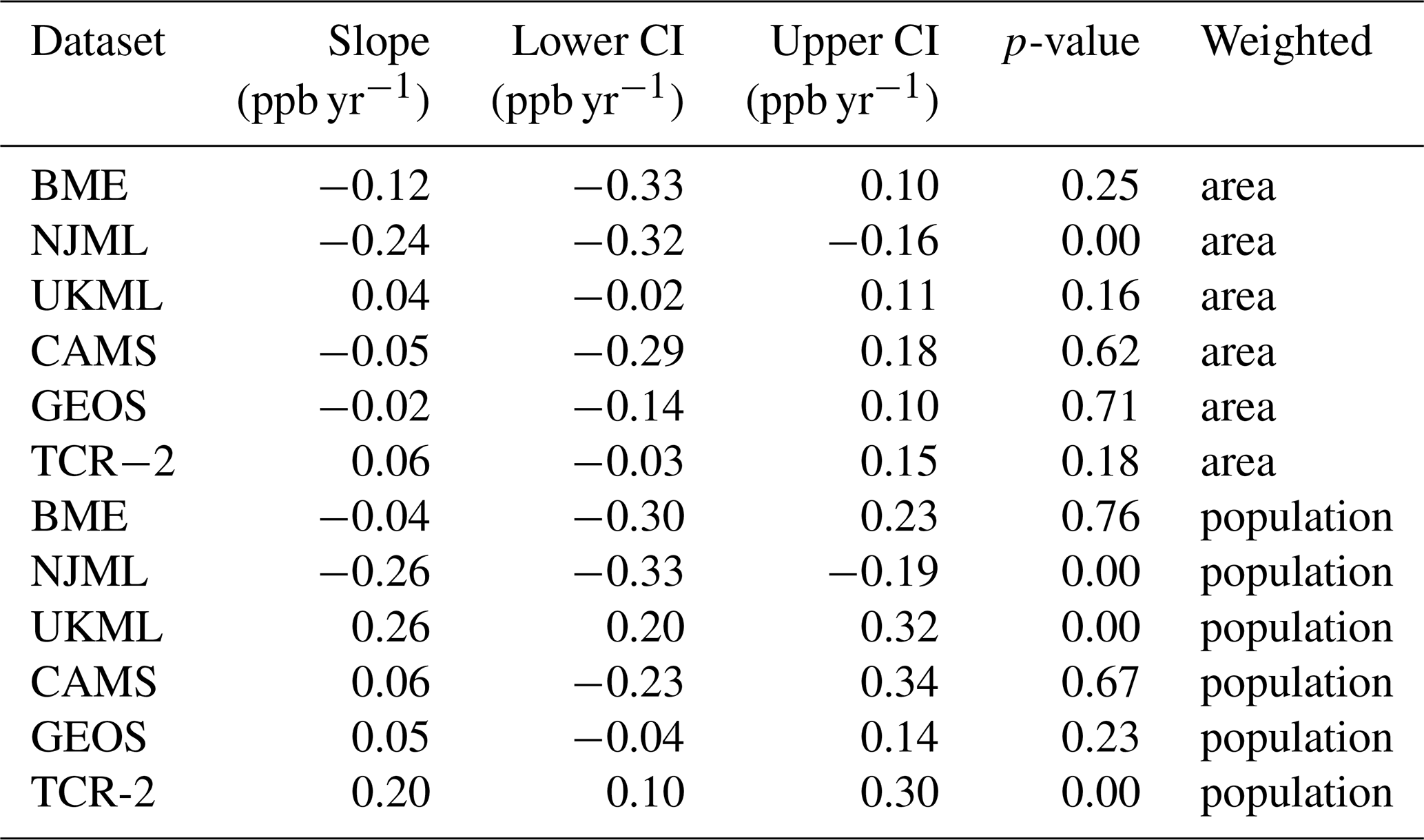
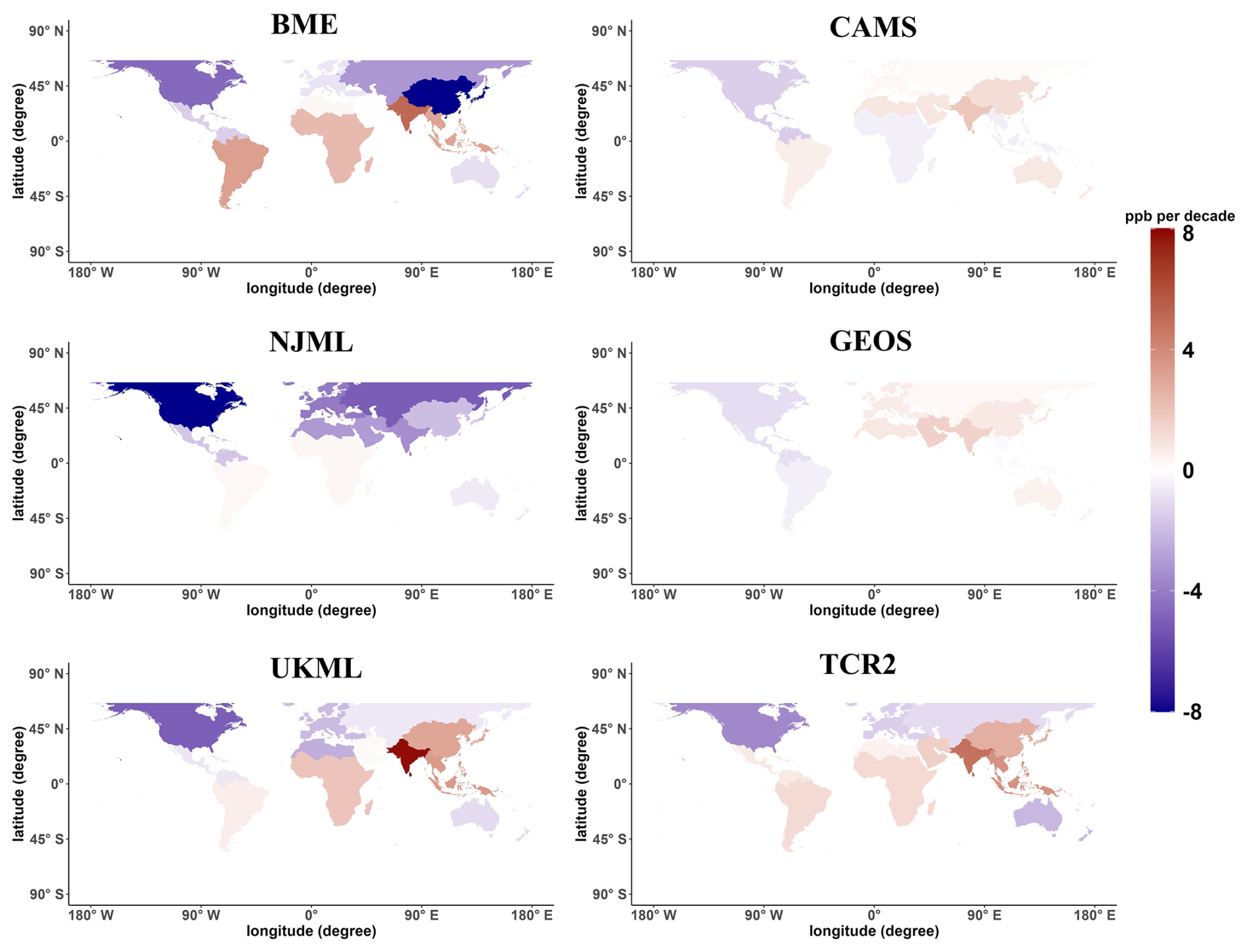
Figure 6 Population weighted ozone (OSDMA8) trends per decade for six datasets, calculated over the 2006–2016 period analyzed for each dataset. The different regions are defined in Table S7. Population weighted yearly trend of six datasets over priority regions (NAM, EUR, SAS, EAS, SEA, SAF, MDE) from 2006 to 2016 with 95 % confidence intervals and p-values is shown in Table S9.

5.2 Difference maps

Figure 7 shows the spatial maps of the 11-year (2006–2016) average of the annual multi-model means of OSDMA8 from the six datasets, and the associated standard deviations. India, China, and the Middle East are estimated to have the world's highest average ozone concentrations, exceeding 50 ppb in the multi-model average. High ozone levels are also found in parts of Europe and the eastern United States. Notably, regions in southern Africa near the Atlantic Ocean emerge as primary areas of ozone pollution, where some locations have average concentrations exceeding 60 ppb. Conversely, the Amazon Basin in South America, Central Africa, and Canada exhibit relatively lower ozone concentrations, with some areas below the WHO 30 ppb guideline. The six datasets show greater variation (high standard deviations above 10 ppb) in South America and Africa, particularly in rainforest regions, compared to North America and Europe, notably since these regions lack ozone monitors. The eastern coast of China also exhibits significant discrepancies with standard deviations above 15 ppb. Detailed plots of the annual multi-model mean of OSDMA8 from the six datasets, and the associated standard deviations for each year (2006 to 2016) are shown in Fig. S9 and Fig. S10. Figure 8 compares the mean ozone concentration for each dataset with the multi-dataset average (Fig. 7a), showing wide variation in the magnitude and spatial distributions of ozone concentrations among the datasets. BME and CAMS display lower values than the average of six datasets in most regions, consistent with Figs. 1 and 5. BME records concentrations higher than average in central South America and central Africa near the Atlantic, while CAMS shows elevated levels in Southeast Asia and along the Middle East coast, contrasting TCR-2's lower coastal and higher inland concentrations. NJML and UKML report above-average values, except for NJML in southern China and UKML near the Sahara Desert and the Indian Ocean. Detailed plots of difference between annual ensemble mean and each dataset estimate for each year (2006 to 2016) are shown in Fig. S11.

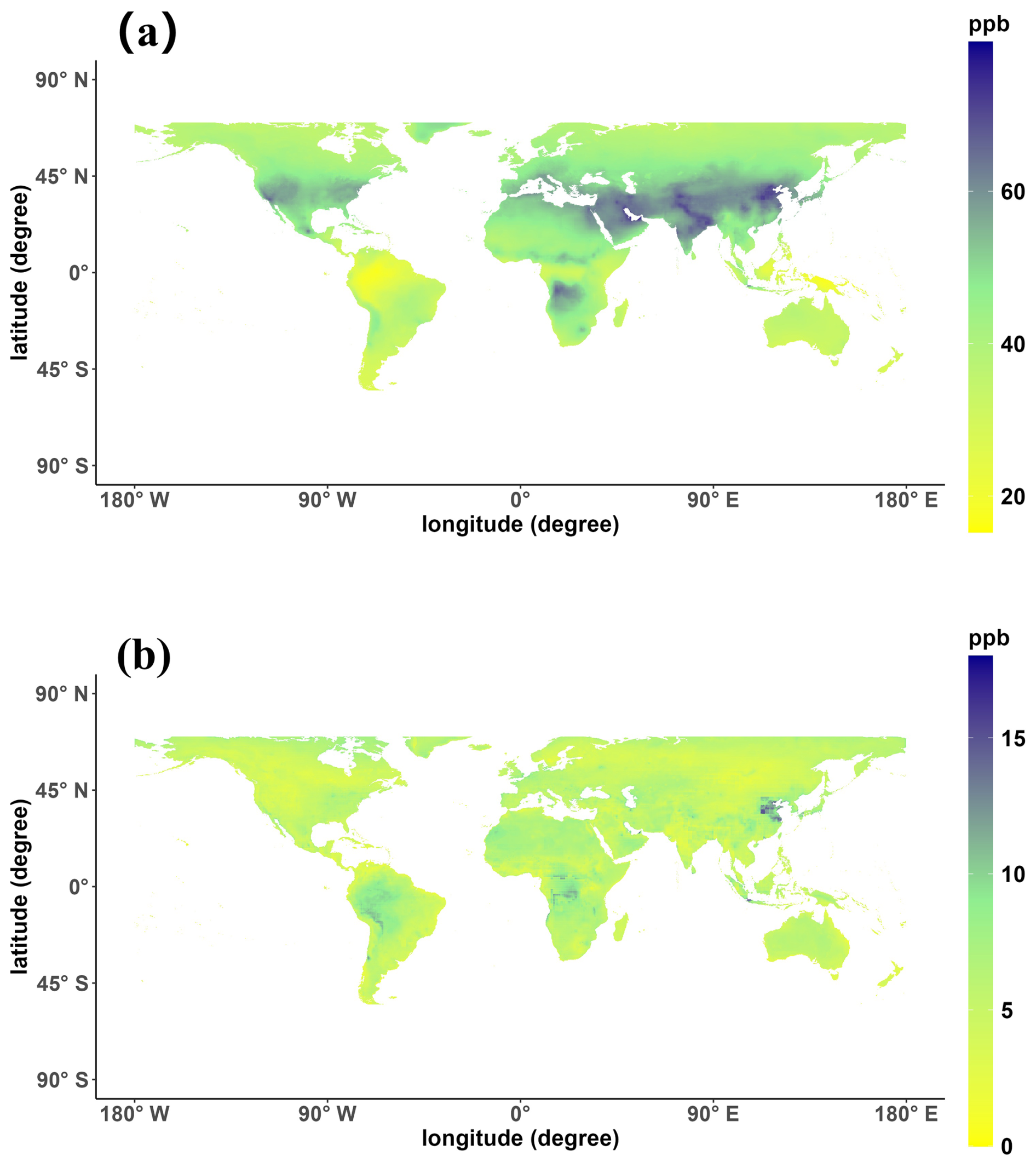
Figure 7 For six datasets from 2006 to 2016, (a) the 11-year ensemble mean, and (b) the average of annual standard deviations. Ozone data are reported as OSDMA8. The mean and standard deviation for each year is shown in Figs. S5 and S6.

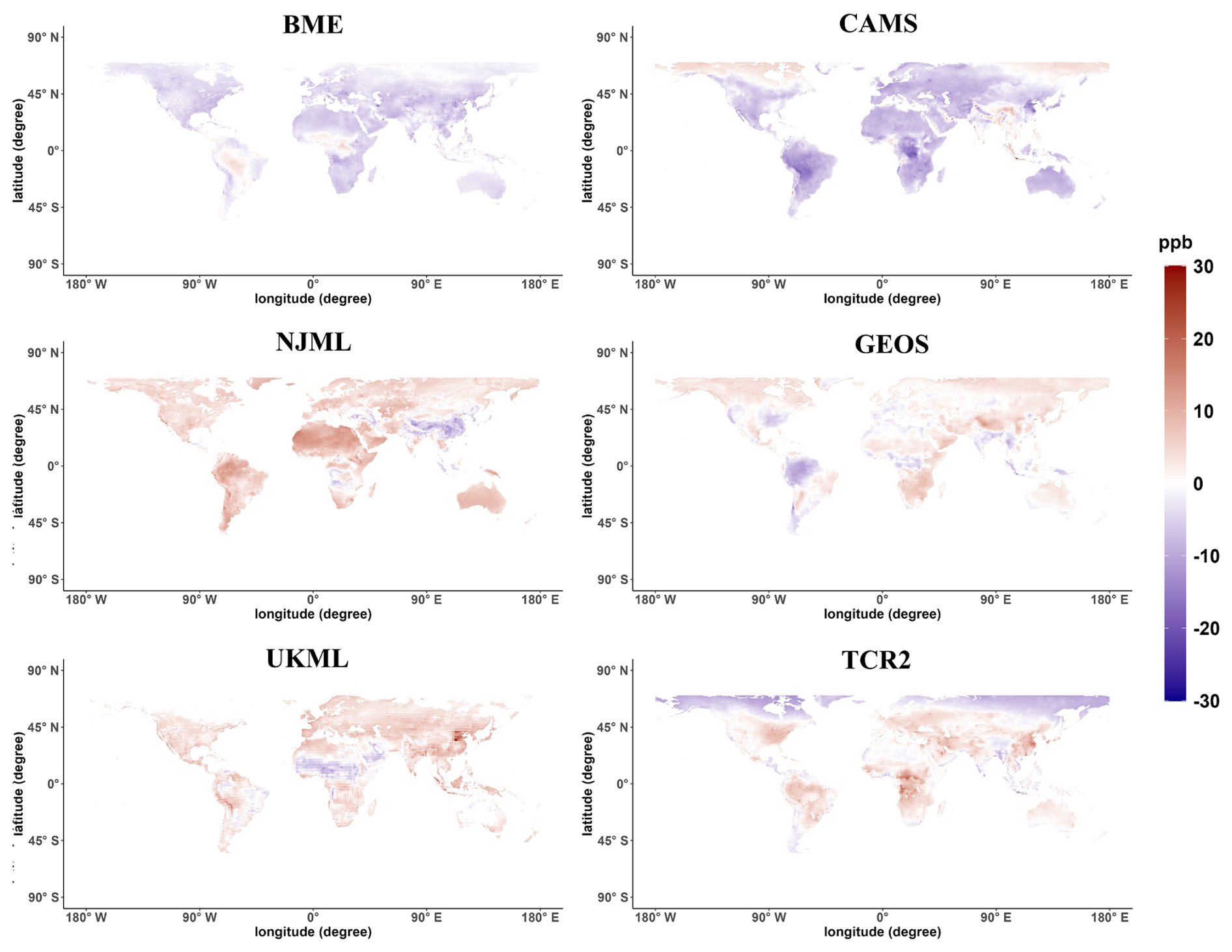
Figure 8 The difference of OSDMA8 in each grid cell between the 11-year (2006–2016) mean of each of six datasets and the ensemble mean (Fig. 3). Positive values indicate that the average estimate of the dataset is higher than the ensemble mean. Negative values indicate that the average estimate of the dataset is lower than the ensemble mean of the six datasets. Difference maps for each year are shown in Fig. S7.

5.3 Pairwise spatial similarity

We calculated the correlation and RMSD between each pair of datasets for each year from 2006 to 2016. Figure 9 displays the average correlation and RMSD values over these 11 years as heatmaps. Figure 9c presents a scatter plot of the correlations and RMSD for each dataset pair. Using the correlation heatmap (Fig. 9a), we categorized the six datasets by the maximum difference method, identifying NJML as a distinct group (Group B) and the other five datasets as Group A. NJML's separation indicates its significant divergence in ozone geographic distribution compared to others. The scatter distribution in Fig. 9c reveals that most Group A data points cluster in regions of high correlation and low RMSD, suggesting broadly consistent ozone geographic distribution and concentration estimates within this group. Nevertheless, there is still substantial disagreement among the reanalysis products, likely because of the differences in forecast model performance and data assimilation configuration. Conversely, Group B has lower correlations. Interestingly, RMSD does not consistently decrease with increasing correlation, indicating that similar geographic distribution patterns can still yield significant differences in ozone concentration estimates. This is particularly evident with CAMS and GEOS-Chem, which exhibit the highest correlation with a large RMSD, suggesting substantial differences in ozone estimation.

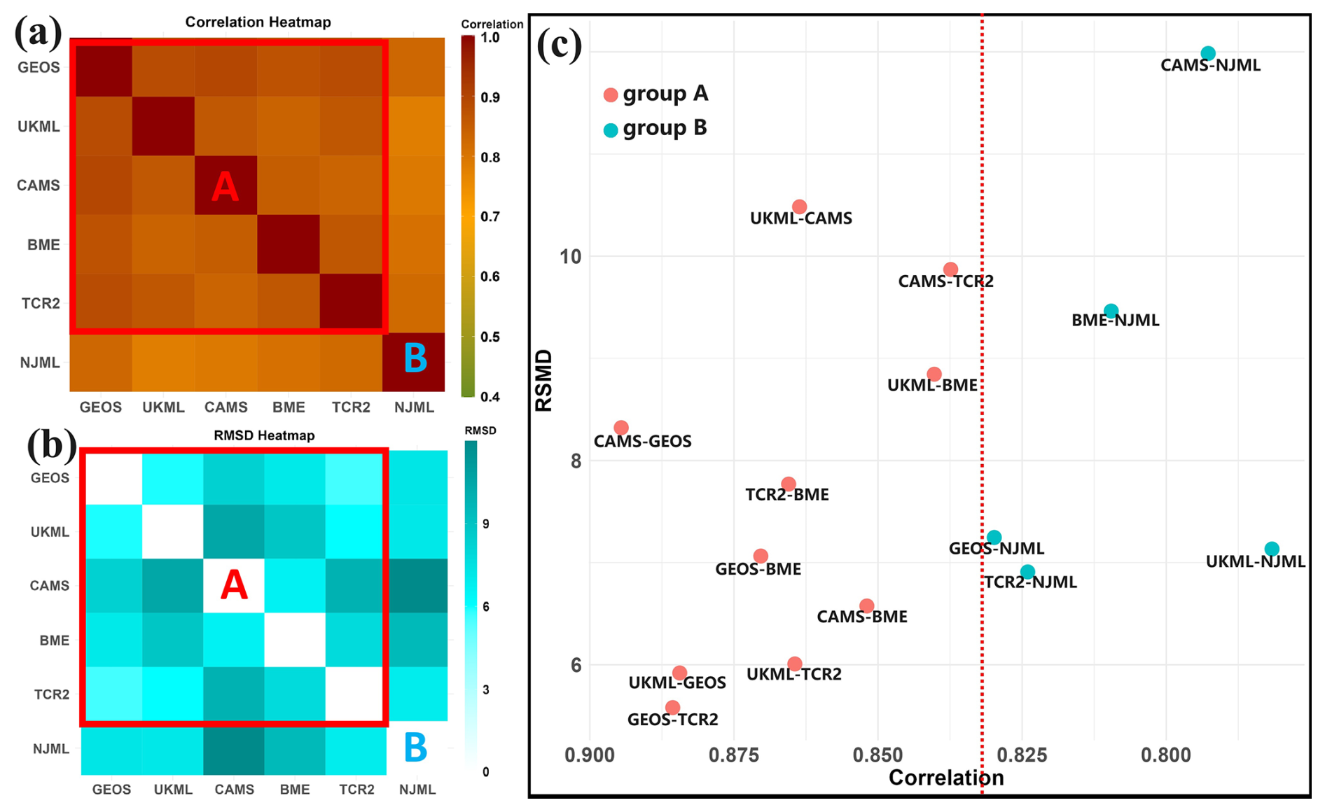
Figure 9 Heatmaps of similarity among the six datasets, including (a) heatmaps of average of pairwise correlation (Pearson R) between each dataset from 2006 to 2016. (b) Heatmaps of average of pairwise Root mean square difference (RMSD) between each dataset from 2006 to 2016. Group A designates five datasets with strong similarity, while Group B is composed of one dataset with lower similarity with the rest. (c) Scatterplot of correlation and RSMD between each pair of datasets. The datasets with greatest similarity are in the lower left of panel (c), and comparisons with the Group B dataset have lower correlation.

5.4 Long-term ozone exposure

Figure 10 illustrates the distribution of population in various regions exposed to average OSDMA8 from 2006 to 2016, as per each dataset. We also calculated the distribution of population regarding the lower and upper bounds of OSDMA8 from 2006 to 2016 for each dataset, as shown in Fig. S12. For the period 2006–2016, a majority of the population in most datasets is exposed to concentrations above 40–50 ppb. Populations in regions such as East Asia and South Asia appear to be exposed to higher ozone concentrations in all datasets compared to other regions, which supports our findings from exposure based on TOAR-II observations in Fig. 3. Conversely, populations in the Sub-Saharan Africa and Southeast Asia regions typically experienced concentrations below 50 ppb. The different regions show different distributions of population ozone exposure, and comparisons between datasets reveal considerable variations in the ozone distribution for each region. Some datasets (e.g., CAMS and TCR-2) show a wider distribution of population across ozone concentrations compared to others (e.g., NJML). In BME and CAMS, after South Asia, a significant fraction of the population in the East Asia region is exposed to levels above 50 ppb, while this proportion in North America, Europe, and the Middle East is less than in the other four datasets. When focusing on exposure above 70 ppb, South Asia dominates in BME, CAMS, and NJML, while East Asia leads in GEOS-Chem, UKML, and TCR-2. All six datasets clearly demonstrate a higher impact of ozone pollution in Asia compared to North America and Europe, aligning with previous findings based on TOAR observations (Chang et al., 2017).

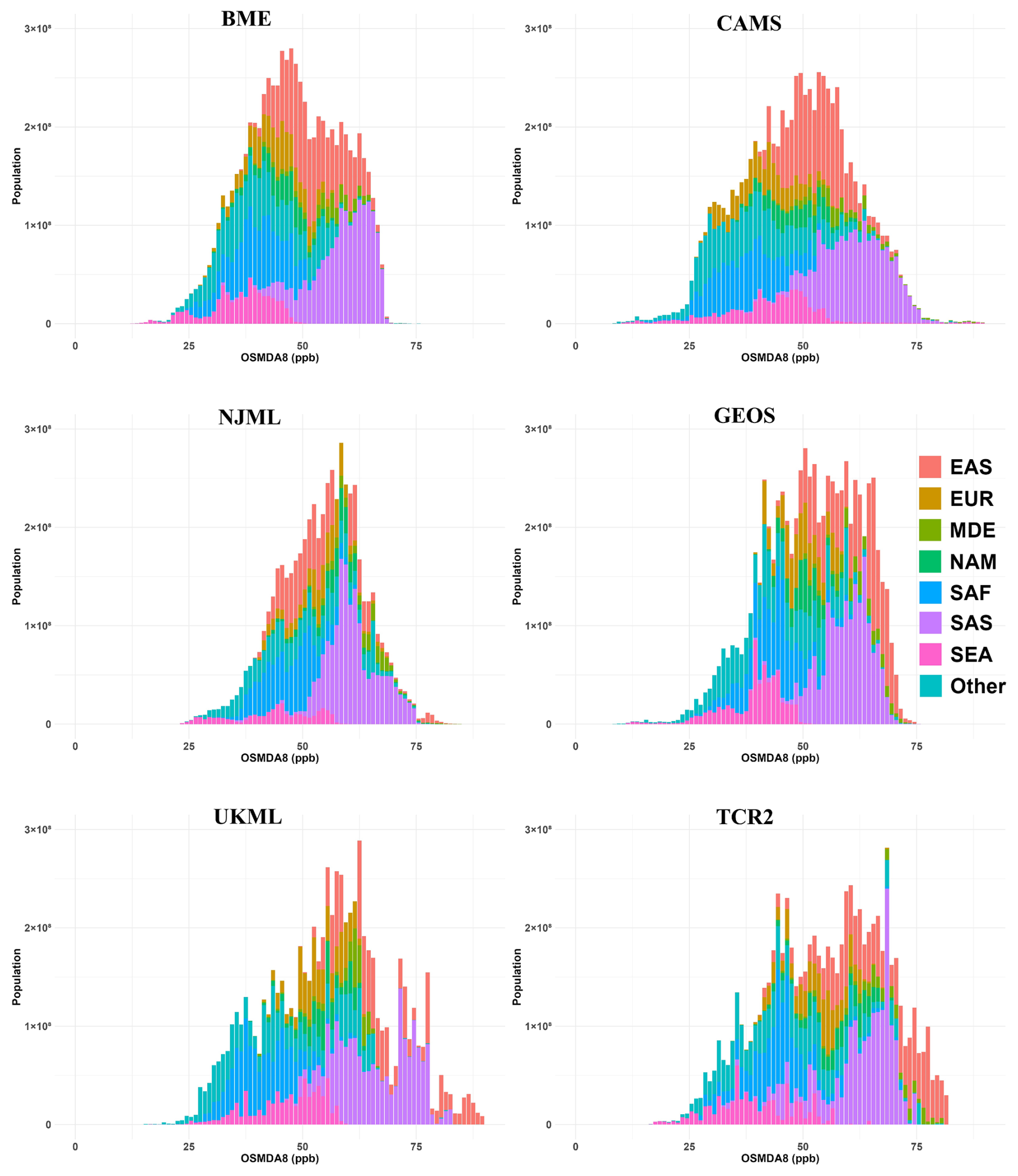
Figure 10 Population exposed to 11-year average ozone (OSDMA8) from 2006 to 2016 in different regions. The horizontal axis represents ozone concentrations, and the vertical axis represents population size. The definitions of different regions are included in Table S7. The Lower and Upper Bound of population exposure, which represent the 95 % prediction interval for the estimate, are presented in Fig. S12.

Table 4 The share of population in percentage (%) exposed to ozone above three particular thresholds (ppb) in each world region, for the 2006 to 2016 average OSDMA8 for six ozone datasets. Each region shows the share of the population exposed at each threshold, calculated using the estimate, the lower bound and the upper bound of the OSDMA8 from each dataset, respectively. The bounds represent the 95 % prediction interval for the estimate, derived from the linear regression of each dataset against TOAR-II observations. Population shares for each year are shown in Table S10. The definitions of different regions are included in Table S7.

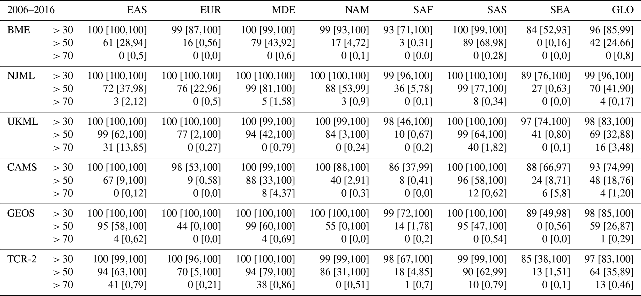
Table 4 elucidates each region's population share above 30, 50 and 70 ppb thresholds from 2006 to 2016. Results are presented as the estimate with the lower and upper bound in parentheses (e.g., 42 % [24 %, 66 %]). Detailed table of population share for each year (2006 to 2016) are shown in Table S10. For BME and CAMS, the global average of the population exposed to more than 50 ppb is 42 % [24 %, 66 %] and 48 % [18 %, 76 %], respectively, indicating that more than half of the population us exposed to lower concentrations. Regional exposure estimates vary in East Asia, where the proportion of the population exposed to more than 50 ppb ranges from 61 % [28 %, 94 %] in BME to 99 % [62 %, 100 %] in UKML, 95 % [58 %, 100 %] in GEOS-Chem, and 94 % [63 %, 100 %] in TCR-2. The differences are stark in Europe, with BME and CAMS showing only 16 % [0 %, 56 %] and 9 % [0 %, 58 %] exposure, respectively, over 50 ppb, while NJML, UKML, and TCR-2 report much higher exposures of 76 % [22 %, 96 %], 77 % [2 %, 100 %], 70 % [5 %, 100 %]. Focusing on the highest threshold, TCR-2 and UKML project that 41 % [0 %, 79 %] and 31 % [13 %, 85 %] of the population in East Asia exposed to levels above 70 ppb, respectively. In the Middle East, TCR-2's estimates are significantly higher than other datasets, indicating that 38 % [0 %, 86 %] of the population is exposed to average concentrations above 70 ppb. Despite these regional differences, the six datasets agree that a large majority of the global population is exposed to ozone above the WHO guideline for OSDMA8 (30 ppb) with percents ranging from 93 % [74 %, 99 %] (CAMS) to 99 % [96 %, 100 %] (NJML).

6 Discussion

When evaluating datasets against TOAR-II observations, differences in performance are seen among six datasets. BME performed well in the TOAR-II evaluation (Fig. 1), with minimal mean bias below the 50 % concentration threshold (Fig. 2). Unlike the other databases, BME tends not to overestimate over the range of concentration, with a small underestimation bias. After removing TOAR sites that were used as inputs to BME (Fig. S13), BME's performance remains robust in both evaluation scenarios. NJML and UKML, both utilizing TOAR-I as a training set, showed overestimation in most areas (Table 2). NJML exhibits a higher R² from 2010 onward, especially at high ground-level ozone concentrations (above 50 ppb), where prediction accuracy generally declines across all datasets. However, NJML has missing data in some coastal regions, particularly in European coastal countries, which may contribute to its elevated RMSE in Europe compared to other datasets (Table 2), since missing data are substituted with the nearest model grid cell. UKML's performance after 2010 is not as good as NJML and is worse than the chemical reanalysis datasets. CAMS, GEOS-Chem and TCR-2 primarily rely on satellite data, suggesting that they might not compare favorably with other datasets that used observations as input or training data. Despite this, the three chemical reanalysis datasets unexpectedly outperform the machine learning datasets in R² (TCR-2, GEOS-Chem) and in RMSE (CAMS) over the full year 2016. In addition, for chemical reanalysis datasets, there is a clear trade-off between capturing the spatial pattern and the accuracy. As shown in Fig. 2, TCR-2, GEOS-Chem all have widespread overestimation, but they often capture spatial patterns more effectively (higher R²). Conversely, CAMS exhibits low bias in RMSE but shows worse spatial correlation in China. All six datasets show a reduced performance at higher ozone concentrations (> 50 ppb), which may complicate their accuracy for assessing long term high-pollution exposure. Furthermore, most datasets perform better in regions with lower monitoring density (e.g., the United States and China) than in those with higher density (e.g., Japan and South Korea), which suggests that resolving high-resolution local ozone distributions remains challenging even with a good amount of observational data. The performance of each dataset impacts the accuracy of trend analysis (Figs. 5 and 6) and population exposure assessment (Fig. 10), shown as uncertainty in these Figures, which may lead to different results when compared to the WHO guideline and interim target.

From the comparison, the large disagreements among the six datasets regarding ozone trends, population exposure, and concentration estimates are a direct consequence of the systematic biases and performance issues identified in the evaluation. Figure 5b illustrates that BME and CAMS report lower ozone estimates compared to UKML and NJML, with differences exceeding 5 ppb. NJML demonstrates a very high certainty decreasing trend in global population-weighted and area-weighted yearly mean over the 2006–2016 period. While TCR-2 and UKML exhibit very high certainty increasing trends in global population-weighted mean which relates to their overestimation. Divergence among datasets becomes even more evident in the analysis of regional ozone trends (Fig. 6). Ozone concentrations decreased in Europe from 2006 to 2016 according to BME, NJML, UKML, and TCR-2, yet increase in the other chemical reanalysis datasets. These uncertainties critically undermine the reliability of population exposure assessment. Among the six datasets, the population exposed to more than 50 ppb of ozone in Europe from 2006 to 2016 spans a broad range, from as low as 9 % for CAMS to over 70 % for NJML, UKML, and TCR-2. In East Asia, exposure levels are consistently higher, with the percentage of the population affected ranging from 61 % for BME to more than 90 % for UKML, GEOS-Chem, and TCR-2 based on average OSDMA8 data over the same period. Global average exposures also vary, with the proportion of the population exposed to more than 50 ppb ranging from 42 % to 70 % across the six datasets. More importantly, the evaluation reveals that all datasets perform poorly at high ozone levels (> 50 ppb). This highlights the importance of removing systematic biases from these data sets before applying them to exposure estimates.

Despite notable disparities in estimates, we still find some regional and temporal similarities across the six datasets. In Fig. 6, all datasets exhibit a downward trend in North America over 2006 to 2016. And from the evaluation, we find that all datasets perform well in the United States, which makes the downward trend more reliable. In Fig. 7a high ozone concentrations are predominantly found in regions with elevated anthropogenic and industrial emissions, while forests and sparsely populated areas have lower ozone concentrations, consistent with findings based on observations (Mills et al., 2018b; Fleming et al., 2018). In Fig. 7b the standard deviation among six datasets is high in part of South America and Africa, especially in the rainforest areas, probably because of the lack of observational data in these areas and uncertainties in the emissions inventories (Pfister et al., 2019). However, for most regions it is low, such as North America and South Asia, indicating a good level of agreement on ozone estimates. The high pairwise correlation in Fig. 9a supports that the geographical distributions of ground-level ozone are similar among most of datasets. The histograms of ground-level ozone exposure among the population (Fig. 10) reveal the shared characteristic of widespread high ozone exposure in East Asia and Southeast Asia (Fleming et al., 2018).

There are several possible explanations for the differences among the datasets, including several factors related to the characteristics, methodologies and input data for each dataset. BME has an unfair advantage in that it nearly matches observations at a monitoring location. But as mentioned earlier, BME still shows superior performance after removing its training data from the evaluation. BME's use of temporal autocorrelation to predict ozone in years where measurements are missing may help its good performance (DeLang et al., 2021). The differing yearly ozone population-weighted mean trend in NJML compared to other datasets may be due to its unique input data, including land cover and satellite observations (Liu et al., 2022a). The missing data near coastlines in NJML and relatively coarse resolution likely contribute to poorer performance in EU-27. For three chemical reanalysis datasets, previous studies have shown that significant challenges remain, particularly with respect to the representation of ozone in the lower troposphere, because of the limited sensitivity of satellite observations to ozone in the lower layers (Huijnen et al., 2020). Because of the lack of direct observational constraints at the surface in the chemical reanalyses, the better performance of CAMS may be attributable to the finer resolution that enables better representation of small-scale ozone distribution features than the other reanalysis datasets, and also to the better performance of the forecast model to predict surface ozone. Nevertheless, the assimilation of precursor measurements provides important constraints, particularly with respect to the spatial gradient and temporal variation of ground-level ozone. The low RMSE of GEOS-Chem compared to UKML and TCR-2 might be because it shares the same data assimilation method with CAMS (Qu et al., 2020a). Moreover, TCR-2, GEOS-Chem, and CAMS perform well in the United States, Canada and EU27, which may be because these regions have well-established emissions inventories for modeling (Schmedding et al., 2020) and because data assimilation is used to estimate key precursor emissions from satellite observations in TCR-2 and GEOS-Chem. Optimizing additional precursor emissions, such as VOCs, from satellite observations is considered to be important to better represent surface ozone (Miyazaki et al., 2019; Sekiya et al., 2025; Miyazaki et al., 2012). The poor performance in South Korea and Japan could be because the coarse resolution models may not accurately capture ozone gradients in a nation with a high density of monitors (Punger and West, 2013; Sekiya et al., 2021). This suggests a need for continued efforts to improve the mapping resolution to capture spatial variability in these regions. Since most of the current reanalysis products still suffer from large systematic errors in their surface ozone analysis, it might be important to apply bias corrections while maintaining the detailed spatial and temporal variability of the original data using methods such as machine learning (Miyazaki et al., 2025) before performing exposure estimates. While these factors may help to explain differences between the datasets, we have not systematically tested them, and as discussed by Sekiya et al. (2025) and Jones et al. (2024), further inter-comparisons of reanalysis products and detailed discussions for improvement are required.

Although we conducted a comprehensive comparison and evaluation, this study still has some limitations. First, the comparison only focuses on land and inhabited islands, because of the focus on ground-level ozone impacts on health. Our estimates of population exposure are based on ambient concentration in each grid cell, ignoring other factors that impact ozone exposure, such as indoor ozone concentration. Also, using OSDMA8 as the metric to evaluate datasets might hide differences in model performance at hourly temporal resolution, which would need to be analyzed in a separate study. In instances of missing model estimates, we default to the nearest valid estimate to evaluate with TOAR-II observations or re-gridded grid cell. For datasets with coarse spatial resolution, this method may increase or reduce bias by double counting.

7 Conclusions

This study evaluates the consistency and accuracy of six ground-level ozone mapping products, developed using different methods. Substantial discrepancies among datasets are reflected in global and regional ozone trends, the spatial distribution of ozone, population exposure estimates, and model performance. Model performance evaluation based on TOAR-II observations varied. BME performs well near monitoring locations with good R² and small RMSE. All five datasets, except for BME, exhibit similar R² values in 2016. NJML performs well after 2010 and shows robust performance under high ozone concentrations. Machine learning datasets tend to overestimate. The chemical reanalysis datasets perform comparably with the geostatistical and machine learning datasets, which is somewhat surprising given that they were not designed to estimate ground-level ozone accurately and do not use ground-level observations as input. CAMS performs the best among the chemical reanalysis datasets in term of RMSE, although CAMS has difficulty capturing TOAR-II observations in China. In regions where TOAR-II observations are sparse, all datasets show RMSE values about 10 ppb, highlighting the difficulty in mapping ground-level ozone magnitude in regions with little observational data. Conversely, in some regions with very dense TOAR-II observations, all datasets show R² values below 0.2, highlighting the necessity for fine resolution mapping to accurately capture spatial variability. The global population-weighted average has a maximum span of 10 ppb among the six datasets. In terms of population-weighted mean trends over 2006 to 2016 period, UKML and TCR-2 show very high certainty upward trends globally, while NJML shows a very high certainty downward trend. Regionally, all datasets show a downward trend in North America, and the evaluation results make this trend more reliable. Only BME and NJML datasets demonstrate a downward trend in East Asia, and they also fit well with TOAR-II observations in population density distribution. In Europe, BME, UKML, NJML and TCR-2 report a downward trend, while the other two chemical reanalysis datasets reveal an upward trend that is not seen in observations. These differences among datasets are sufficiently large that assessments of health impacts of ozone would differ significantly when using different ozone datasets.

Given that some of the datasets used similar input data, it is somewhat surprising to find the large discrepancies shown here, suggesting that applications of these datasets to health burden assessments, epidemiology or similar applications for agricultural and ecosystem impacts may differ strongly based on the dataset selected. The coarse-resolution datasets, GEOS-Chem and TCR-2, perform well in grid-to-grid evaluations at their native resolutions, making them effective for studying long-term regional ozone effects. However, because of their coarser resolutions, these two datasets cannot capture site-level distributions and exhibit greater bias than the higher-resolution BME, CAMS, and NJML datasets. UKML, despite its relatively fine resolution (0.125°), shows larger biases and a lower R². The superior performance of BME and NJML should be noted with the fact that both datasets use observational data for input or training, which gives them an inherent advantage in these evaluations. More research will be needed before different methods converge on similar estimates. Such research can include more widespread ground observations, improved used of satellite observations, improved chemistry-climate modelling, and further development of different data fusion methods. Also, it is not clear whether differences among datasets are due mainly to the methods used or to differences in input data. In addition, establishing a formal benchmark test based on the evaluation methods described in this study for the yearly OSDMA8 metric is essential. This would allow for new mapping products to be easily assessed. The general findings here of poor agreement among datasets may also be applicable to other air quality datasets or even datasets from other Earth system domains. According to this study, there is no clear consensus on the best ozone mapping methods. To further improve these ozone mapping products, researchers must update and adjust their methods and input data regularly and iteratively.