Development of a parametrised atmospheric NO_x chemistry scheme to help quantify fossil fuel CO₂ emission estimates

Success of the Paris Agreement relies on rapid reductions in fossil fuel CO₂ (ffCO₂) emissions. Atmospheric data can verify the ffCO₂ reductions pledged by nations in their nationally determined contributions. However, estimating ffCO₂ from atmospheric CO₂ is challenging due to natural fluxes and varying backgrounds. One approach is to combine with nitrogen oxides (NO_x = NO + NO₂), which are co-emitted with CO₂ during combustion. A key challenge in using NO_x to estimate ffCO₂ is the computational cost of modelling atmospheric photochemistry. Additionally, the NO₂ : NO column ratio must be well understood to convert model NO_x columns to NO₂ columns for comparison with satellite data. We use random forest regression to parameterise NO_x chemistry, relying only on meteorological parameters and NO_x concentration. The regression is trained on outputs from a nested GEOS (Goddard Earth Observing System)-Chem model simulation for mainland Europe in 2019. We develop a monthly NO_x chemistry parameterisation that performs well when tested on perturbed emission runs (R² > 0.95) and on unseen meteorology for 2021 (R² > 0.79). We also parameterise the NO₂ : NO ratio (R² > 0.99 on perturbed outputs, R² > 0.92 on unseen meteorology). Additionally, we present an alternative method to predict NO_x rates by scaling baseline NO_x rates with changes in NO_x concentration (R² = 1.0 on perturbed outputs). Our models reproduce NO₂ columns with minimal deviation from full-chemistry models, with reconstruction error smaller than the TROPOspheric Monitoring Instrument (TROPOMI) precision in over 99.9 % of cases, supporting robust ffCO₂ inversion efforts. These results provide a robust framework for accurately estimating fossil fuel CO₂ emissions from atmospheric data, enabling more reliable monitoring and verification of global emissions reductions.

1 Introduction

Reaching net zero greenhouse gas emissions is a global goal, needed to curb further warming of our planet. Achieving that goal on a national scale requires accurate knowledge about fossil fuel emissions of CO₂ (ffCO₂) to verify a country's progress towards achieving their Nationally Determined Contributions under the Paris Agreement. But how can a country assess whether they are heading in the right direction? The default approach is to use national inventories that are compiled from energy statistics and emission factors but they are uncertain for various reasons, mainly associated with the veracity of the statistics and their spatial and temporal distributions and the default assumption of time-invariant emission factors (Kuenen et al., 2014; Hoesly et al., 2018b). Such “bottom-up” inventories are typically available with a delay of 2 years (Janssens-Maenhout et al., 2019) thereby introducing a temporal disconnect between climate action and results. The alternative “top-down”, data-driven approach uses Bayes' theory to infer CO₂ emission estimates from observed changes in atmospheric CO₂. This approach is also subject to uncertainties including errors in atmospheric transport models, sparse observational coverage, and background concentration estimation (Peylin et al., 2013; Andrew, 2020). One of the remaining challenges associated with this atmospheric approach is isolating the combustion and natural contributions to atmospheric CO₂ (Oda et al., 2023). Various approaches have been proffered to address that challenge, which fall into two broad categories: spatial disaggregation of combustion (Shu and Lam, 2011; Liu et al., 2018) and natural fluxes and using an additional trace gas (Meijer et al., 1996; Lopez et al., 2013; Wenger et al., 2019; Super et al., 2020), associated exclusively with combustion or natural processes common to CO₂. One such trace gas is NO_x, but due to the large computational overhead of directly modelling the atmospheric NO_x photochemistry, we endeavor to determine an alternative methodology to model NO_x chemistry. Here we describe a parameterisation of tropospheric nitrogen oxide (NO_x = NO + NO₂) chemistry that effectively unlocks our ability to use NO_x alongside CO₂ to quantify ffCO₂ estimates within an Bayesian inference framework, particularly in the context of an operational system.

Extracting energy from carbon-based fuels relies on breaking apart atomic bonds that form the molecular structure of the fuel, thereby releasing energy. This is achieved by combustion in which the fuel, composed primarily of hydrogen-carbon bonds, is oxidized by molecular oxygen (O₂). Generally, more energy is released during combustion for fuels with a higher H : C ratio. The primary products of combustion are CO₂ and water vapour. However, when combustion is inefficient – for example, due to insufficient O₂ to fully oxidise the fuel – a wider range of compounds is released, depending on the composition of the fuel being burned. For many combustion processes, air is used to provide O₂. While molecular nitrogen (N₂) in air does not take part in the combustion reaction, the high temperatures involved can thermally dissociate N₂ to facilitate the production of NO (and to a lesser extent NO₂), which is subsequently co-emitted with the CO₂ emissions. The advantage of using atmospheric NO_x as a tracer of ffCO₂ is its relatively short lifetime, on the order of hours to days, which means that we can link elevated NO₂ satellite columns directly to their parent NO_x emissions. Numerous studies are using observations of NO_x and NO₂ to constrain estimates of ffCO₂ (Berezin et al., 2013; Lopez et al., 2013; Goldberg et al., 2019; Super et al., 2020). With the increasing availability of in situ and satellite measurements of atmospheric CO₂, NO₂ and other fossil-fuel tracers, deriving ffCO₂ through multi-species model inversion techniques is becoming a widely used approach (Feng et al., 2009; Nayagam et al., 2023; Super et al., 2024; Wang et al., 2025). However, a key limitation of this method is the uncertainty in CO₂ : NO_x emission ratios, which vary by sector, fuel type, and combustion technology (Jiang et al., 2010; Wang et al., 2025) . Additional challenges include errors in atmospheric transport modelling, accurate representation of chemical processes, and limited observational coverage.

We present a methodology for parameterising NO_x chemistry to reduce the associated computational overhead. We consider NO_x because its constituents, NO and NO₂, rapidly interconvert (Jacob, 1999). By modelling NO_x as a proxy for the combined NO and NO₂ we can save a considerable amount of computational time that would otherwise be spent on photochemical calculations (previously shown in Wu et al., 2023). To do this we need a model that can predict the net loss of NO_x at each time step and grid point. The rate of decay of NO_x is driven by a number of meteorological parameters (Nguyen et al., 2022) including, but not limited to, the irradiance from sunlight, air temperature and solar zenith angle. In this study, we develop a machine learning-based random forest regression model, trained on a full-chemistry version of the GEOS (Goddard Earth Observing System)-Chem atmospheric chemistry model, to accurately predict the atmospheric NO_x rate of change using a small set of driving variables. We evaluate the robustness of our parameterised NO_x chemistry using perturbed emissions on the order of those we typically employ in ensemble Kalman filter techniques. With atmospheric inversion methods in mind, atmospheric NO_x emission estimates tend to be constrained by satellite column observations of NO₂ (Napelenok et al., 2008; Zhao and Wang, 2009; Kemball-Cook et al., 2015) so our parameterised model must also be able to describe changes in NO₂. We achieve this by developing a further random forest-based model, which can predict the species concentration NO₂ : NO ratio.

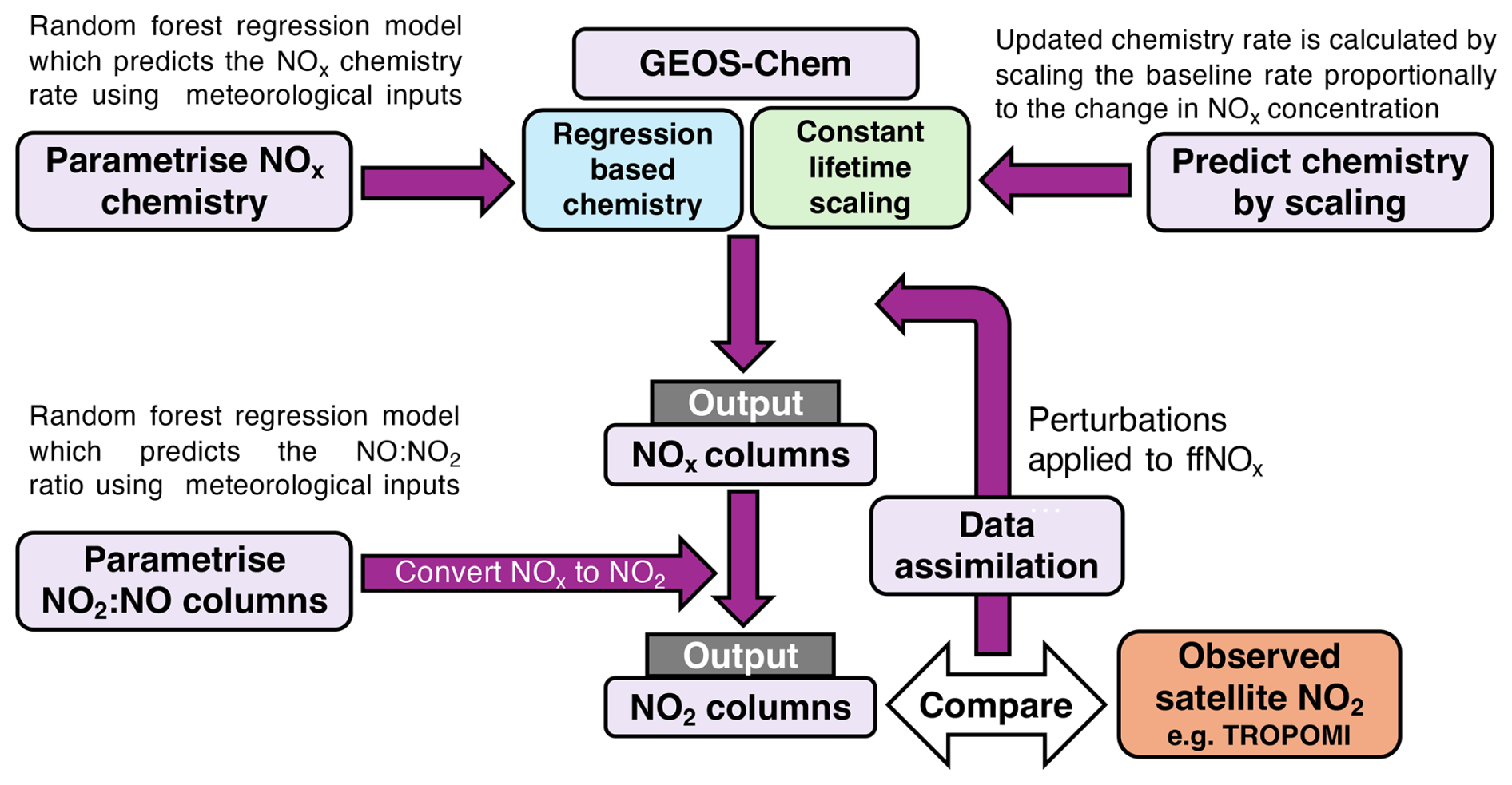
Figure 1 A schematic illustrates how NO_x chemistry parameterisation models are integrated into GEOS-Chem for modelling of atmospheric NO_x without a full chemistry scheme.

Figure 1 shows a schematic overview of the steps used to parameterise NO_x chemistry and partitioning for efficient modelling of NO₂ columns. The first stage involves running atmospheric simulations of NO_x using offline chemistry rates, which are either predicted by random forest models (described in Sect. 2.2) or estimated through relative scaling (described in Sect. 2.3). In the second stage, the NO_x output from these simulations is converted to NO₂, enabling direct comparison with satellite observations such as TROPOMI NO₂. This approach provides an efficient framework suitable for data assimilation applications.

In the next section, we describe the GEOS-Chem atmospheric chemistry transport model that we use to train our random forest models, the satellite observations of column NO₂ that we use to evaluate our parameterised atmospheric chemistry model for NO₂, and the approach we take to construct the random forest model. In Sect. 3, we report the performance of random forest models of atmospheric NO_x and NO₂ : NO, and evaluate the corresponding atmospheric NO₂ columns using satellite data. We conclude the paper in Sect. 4.

2 Data and methods

Here, we describe the GEOS-Chem atmospheric transport model used to build our random forest regression models, the satellite column data we use to evaluate our parameterised model of atmospheric NO_x chemistry, and details that describe how we develop our random forest regression models. A random forest regression model, or a constant lifetime scaling based approach can be used to predict the chemistry rates. The modelled NO_x concentrations are then converted to NO₂ using an additional random forest model. This efficient approach significantly reduces GEOS-Chem's computational cost for forward modelling of NO₂ columns. This is particularly useful for high resolution data assimilation, allowing anthropogenic NO_x emission perturbations to be compared with satellite NO₂ observations, such as the TROPOspheric Monitoring Instrument (TROPOMI).

2.1 GEOS-Chem atmospheric chemistry transport model

We use version 14.2.2 of the GEOS-Chem atmospheric chemistry transport model (Bey et al., 2001) to describe the emissions, transport, and chemical production/loss of atmospheric NO_x. For the purpose of our study, we use a nested version of the full chemistry model, centred over mainland Europe (32.75 to 61.25° N, −15 to 40° E) with 47 vertical levels, approximately 30 of which fall below the dynamic tropopause, where the first model layer has a depth of 130–180 m. The nested model runs with a horizontal spatial resolution of 0.25° × 0.3125°. Initial conditions and lateral boundary conditions to the nested domain were created from a consistent global version of the GEOS-Chem model run at 4° × 5°, with three-hourly output fields. We ran the model with a transport timestep of 5 min and a chemistry timestep of 10 min.

The model is driven by offline meteorology fields from the GEOS Forward Processing (GEOS-FP) product from the Global modelling and Assimilation Office (GMAO) at NASA Goddard Space Flight Center. GEOS-FP has a native horizontal resolution of 0.25° × 0.3125° with 72 vertical pressure levels and 3 h temporal resolution. To describe the emissions of NO_x we used anthropogenic emissions from the Community Emissions Data System (CEDS) version 2 (Hoesly et al., 2018a, b), which provides NO emissions for anthropogenic combustion (industry, energy extraction), and non-combustion sources (agriculture, solvents), including surface transport and shipping. Aircraft emissions for NO and NO₂ are taken from the Aviation Emissions Inventory Code (AEIC) (Simone et al., 2013). Pyrogenic emissions of NO are taken from the Global Fire Emissions Database (GFED) version 4.1 (Randerson et al., 2017).

GEOS-Chem's full-chemistry mechanism simulates atmospheric chemistry by explicitly solving a comprehensive network of chemical reactions, capturing the production, transformation, and loss of NO_x and related species. NO_x chemical loss is simulated through key reactions such as NO₂ reacting with ozone (O₃) to form NO₃, hydroxyl radicals (OH) to produce nitric acid (HNO₃), and hydroperoxyl radicals (HO₂) to form peroxynitric acid (HNO₄). Organic nitrate formation is included through the reactions of NO₂ with methyl peroxy radicals (MO₂) and methacryloyl peroxy radicals (MCO₃), forming methyl peroxy nitrate (MPN) and peroxyacetyl nitrate (PAN), respectively. Additional loss occurs via NO₃ reacting with NO₂ to produce dinitrogen pentoxide (N₂O₅). Simultaneously, the model accounts for important regeneration pathways, including the thermal decomposition of N₂O₅ into NO₃ and NO₂, the breakdown of PAN to release NO₂ and methacryloyl peroxy radicals (MCO₃), and the photolysis of HNO₄ to produce NO₂ and HO₂. Rapid NO to NO₂ exchange is simulated through key reactions, including NO + O₃ → NO₂ + O₂, which relies on ozone to oxidize NO, and NO + NO₃ → 2 NO₂, which occurs through the reaction of nitric oxide with nitrate radicals. Additionally, photochemical reactions driven by sunlight include NO₂ + O₂ + hv → NO + O₃, where nitrogen dioxide photodissociates to form nitric oxide. The mechanism determines reaction rates using reaction rate coefficients that depend on temperature, pressure, and solar radiation, alongside environmental inputs like meteorological fields and species concentrations.

The average diurnal cycle of NO_x chemical rate of change calculated from full-chemistry simulations is presented in Fig. A1 for the four seasons of the year. The shape of the diurnal cycle in the NO_x tendency varies seasonally, influenced by changing sunlight intensity and atmospheric conditions. In winter, the net NO_x loss peaks predominantly at night, when photolytic regeneration ceases and reservoir species like HNO₃ and PAN accumulate, removing NO_x from the reactive pool. During spring and autumn, while a nighttime peak loss remains, there is an additional peak of comparable magnitude in the morning around 09:00–10:00 local solar time (LST). In summer, the maximum net loss shifts to the early morning hours 07:00–08:00 LST, likely driven by rapid photochemical activity as sunlight increases. Meanwhile, by the afternoon we find episodes of net NO_x production, reflecting stronger photolytic regeneration under high solar intensity. These seasonal and diurnal variations reflect complex interactions between photochemistry, emission patterns, and atmospheric transport, resulting in shifts of NO_x sinks and sources throughout the day and year.

Table 1 Input parameters selected through forward feature selection for random forest regression models predicting the NO_x chemical net rate of change [molec. cm⁻³ s⁻¹] and the NO₂ : NO partitioning ratio.

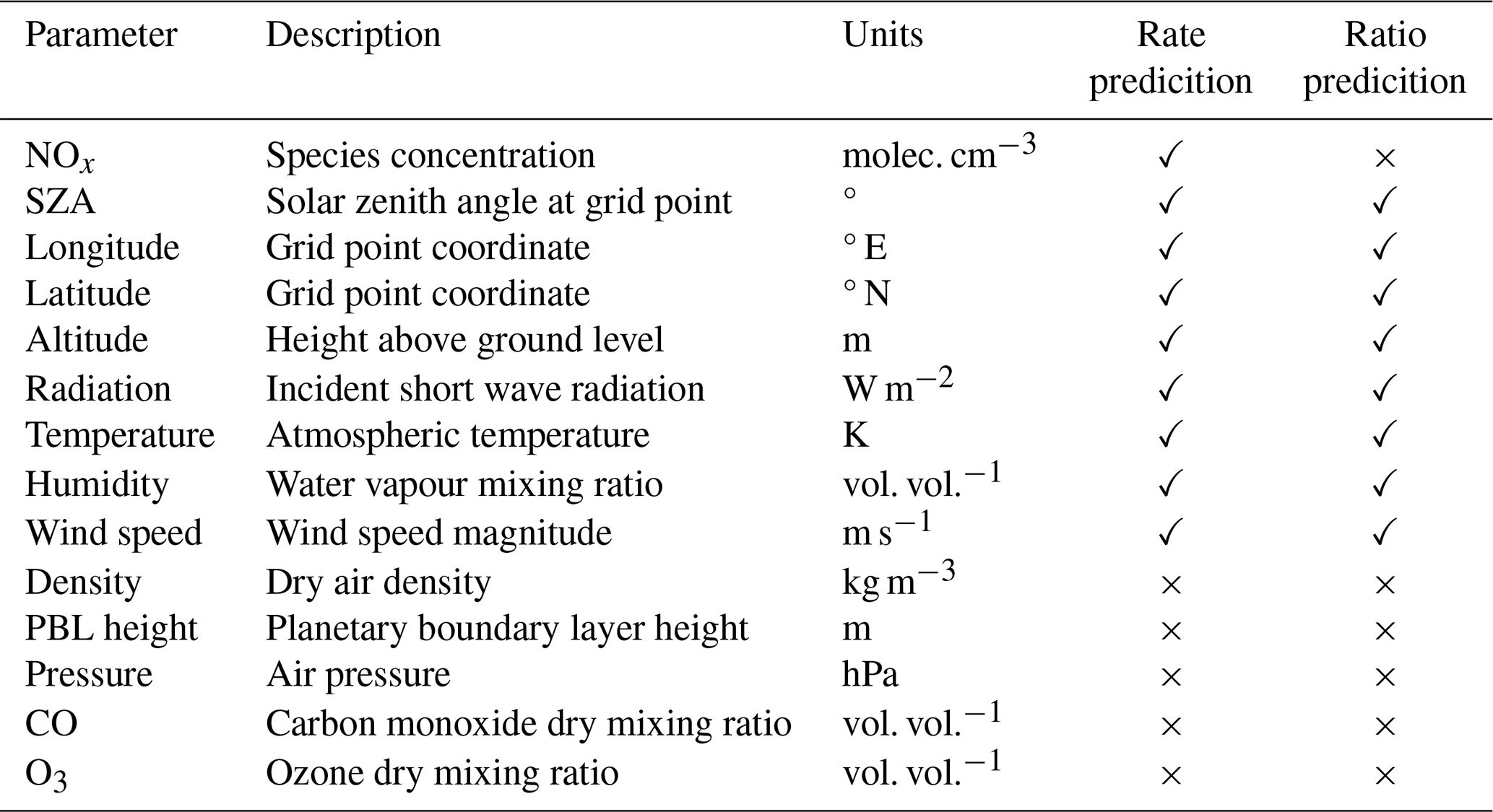
The NO_x concentration, the NO_x chemical rates of change, and relevant meteorology were output at a temporal resolution of one hour. The chosen meteorological parameters are shown in Table 1. These were selected as they were all found to have a relationship with the net NO_x chemical rate of change.

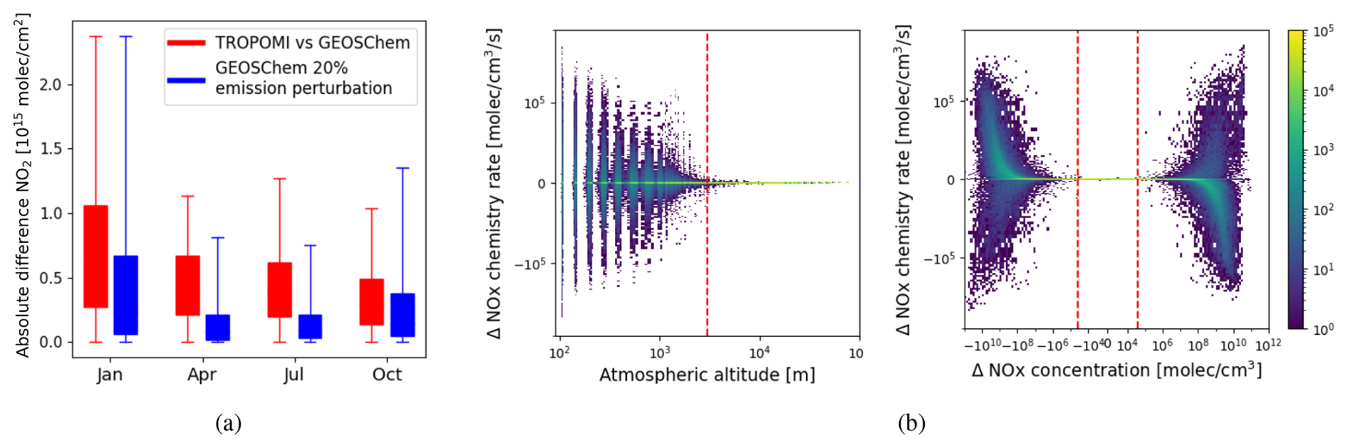
Figure 2 (a) Sensitivity testing shows that the impact of 20 % emission perturbations on modelled NO₂ columns is on the same order as the deviations between GEOS-Chem and TROPOMI. (b) The impact of emission perturbations on the NO_x chemistry rate becomes negligible (< 1 % change, or ΔNO_x rate < 9 × 10³ molec. cm⁻³ s⁻¹) above 3 km from the ground. Additionally, chemistry rate change is negligible in all cases where ΔNO_x concentration < 5 × 10⁴ molec. cm⁻³.

The model was run for the full year 2019 with baseline (unperturbed) NO_x anthropogenic emissions taken from the CEDs emission inventory. This data was used to train the regression models. To further validate the regression model's performance under varying emissions, additional model runs were conducted with random perturbations applied to anthropogenic NO_x emissions on the order of ±20 %. We chose this size of perturbation because a 20 % increase in emissions induces changes in NO₂ columns on the same order of magnitude as the difference observed between GEOS-Chem and TROPOMI (as in Fig. 2a). These perturbed runs were performed for 10 d in January, April, July, and October. A model run for the year 2021 was also performed in order to test the regression performance for an unseen meterological period.

2.2 Random Forest regression modelling

We trained two random forest regressor models to predict the NO_x net chemical rate of change, and the NO₂ : NO partitioning ratio. Random forest models are an ensemble machine learning method, which combine the predictions of many decision trees to improve accuracy and reduce overfitting (Breiman, 2001). A decision tree is a simple predictive model that makes a series of splits in the data based on input variables. At each node, the algorithm chooses the predictor and threshold that best separate the data with respect to the target, continuing until each final branch (or “leaf”) gives a prediction. While a single tree is easy to interpret, it can overfit the data. Random forests address this by building a “forest” of many trees, each trained on a random subset of the data and predictors. This randomness ensures the trees capture diverse patterns, and averaging their outputs yields more robust predictions. Such an algorithm is well-suited to this study as, unlike traditional regression approaches, it does not require assumptions about linearity and can flexibly capture complex relationships and interactions between meteorological drivers and chemical tendencies. Additionally, random forests are relatively computationally efficient to train and can handle correlated predictor variables, making them well suited for large atmospheric datasets.

These models were built using the Sci-kit learn python package (Pedregosa et al., 2011). We evaluated model performance using the coefficient of determination (R²), which quantifies the proportion of variance explained by the model; the mean absolute error (MAE), which measures the mean magnitude of prediction errors; and the mean bias, which indicates the mean tendency of the model to overpredict or underpredict relative to observations. These are defined by the following equations, where y_i are true values, ${\widehat{y}}_i$ are predicted values, $\stackrel{\mathrm{‾}}{y}$ is the mean of the true values, and N is the number of datapoints:

$$\begin{array}{}\text{(1)}& \begin{array}{rl}& R^{\mathrm{2}}=\mathrm{1}-{\displaystyle \frac{{\sum }_{i=\mathrm{1}}^N{\left(y_i-{\widehat{y}}_i\right)}^{\mathrm{2}}}{{\sum }_{i=\mathrm{1}}^N{\left(y_i-\stackrel{\mathrm{‾}}{y}\right)}^{\mathrm{2}}}}\\ & \text{MAE}={\displaystyle \frac{\mathrm{1}}{N}}\sum _{i=\mathrm{1}}^N\left|y_i-{\widehat{y}}_i\right|\\ & \text{Mean Bias}={\displaystyle \frac{\mathrm{1}}{N}}\sum _{i=\mathrm{1}}^N\left(y_i-{\widehat{y}}_i\right)\end{array}\end{array}$$

We separately trained both regression models for each month of the year, for which we report results from January, April, July, and October 2019. The models were developed using the NO_x concentration, the spatial location and a range of meteorological variables as input parameters. We considered a total of 14 input parameters as predictors in the models, shown in Table 1.

To identify the most relevant features for the models, we performed a comprehensive forward selection wrapper procedure, which iteratively adds the feature that yields the largest improvement in mean absolute error until no further gain is observed. Figure A2a and b detail how the performance of the models changed as we added features for the prediction of chemistry rate and the partitioning ratio, respectively. Based on this procedure, we selected a set of nine features for the chemistry rate model, and eight features for the partitioning ratio model (presented in Table 1). Five of the parameters; air pressure, air density, height of the planetary boundary layer, and the mixing ratio of ozone (O₃) and the mixing ratio of carbon monoxide (CO), were consistently excluded from all models during feature selection. The respective importance of each feature across both models for the 4 months studied are plotted in Fig. A2c. For the chemistry rate prediction, the NO_x concentration and the solar zenith angle are consistently emerge as the most important predictorss, contributing around 70 % of the total feature importance in the model. In the ratio prediction, solar zenith angle, altitude, and temperature are the primary predictors during the colder months (January and October), while temperature alone serves as the dominant predictor in the warmer months (April and July). Additionally, the impact on model performance of removing each of the 14 parameters in turn is presented in Fig. A2d. The individual relationship between the nine selected predictors and the NO_x chemistry rate of change are shown in Fig. A3.

To avoid unnecessarily complex models, we tuned the model hyperparameter values to optimise the trade-off between computational efficiency and prediction accuracy. Specifically, we conducted a grid search across the four main hyperparameters in the random forest regression model: the number of trees (estimators), maximum tree depth, maximum number of leaf nodes, and maximum number of features considered at each split. We selected each hyper-parameter as the value at which performance plateaued, defined here as the point beyond which further increases in the parameter resulted in less than a 2 % improvement in model performance. The results of the tuning are presented in Fig. A4. The final optimised model achieved a prediction time of 6 ms per sample, providing a good balance between accuracy and computational cost. In addition to reducing computational time, simplifying the random forest by limiting tree complexity and number also reduces the risk of overfitting, thereby improving the generalisability of the model to new data.

We trained and tested our NO_x chemistry regression models on model grid points in the first 3 km above the surface – the region where changes to surface emissions were found to directly influence the atmospheric chemistry, see Fig. 2b. The regression model for the NO₂ : NO ratio was predicted for each level in the troposphere, and trained on the subset of model data that coincides with the TROPOMI swath (11:30–15:30 LST overpass). The NO₂ : NO ratio can be used to convert the concentration of NO_x to NO₂:

$$\begin{array}{}\text{(2)}& {\mathrm{NO}}_{\mathrm{2}}={\mathrm{NO}}_x{\displaystyle \frac{{\mathrm{NO}}_{\mathrm{2}}:\mathrm{NO}}{\mathrm{1}+{\mathrm{NO}}_{\mathrm{2}}:\mathrm{NO}}}.\end{array}$$

To evaluate model generalisability, we tested model performance using two complementary approaches. Primarily, we assessed predictions on unseen emission perturbation scenarios while holding meteorology fixed. Specifically, we focused on ±20 % emission perturbations similar to those used in ensemble Kalman filter applications (Feng et al., 2009, 2023). This isolates the model's responsiveness to emission changes under consistent atmospheric conditions and reflects its intended use in inversion frameworks, where emissions are perturbed while meteorology remains prescribed. In addition, we include in the appendix (Fig. A6) an evaluation on an entirely independent simulation run for the year 2021, representing unseen meteorological conditions due to its different temporal period. For both approaches, training and testing datasets were constructed via random sampling across all spatial locations and time steps. The training set comprised a random 10 % subset of the unperturbed data, while the test set comprised 0.25 % of the perturbed (or 2021) data, ensuring minimal overlap in specific spatiotemporal conditions. Combined, this dual testing strategy rigorously evaluates the models' ability to generalise across both emission changes and meteorological variability, providing confidence in their performance for atmospheric inversion applications.

2.3 NO_x chemical lifetime

In an alternative formulation, we apply the assumption that the effective lifetime of atmospheric NO_x remains constant under stable meteorological conditions. Hence, if a full chemistry model run is available for a baseline emission scenario, the chemistry rates for perturbed scenarios can be calculated by scaling the original rate according to the proportional change in NO_x concentration. This approach serves as an alternative to using regression models for predicting the chemistry rates.

The effective atmospheric lifetime, τ of NO_x is given by:

$$\begin{array}{}\text{(3)}& \mathit{\tau }={\displaystyle \frac{{\mathrm{NO}}_x}{R_{{\mathrm{NO}}_x}}},\end{array}$$

where NO_x denotes the combined NO and NO₂ species concentrations [molec. cm⁻³] and $R_{{\mathrm{NO}}_x}$ is the instantaneous chemical rate of net loss [molec. cm⁻³s⁻¹], which accounts for the balance between its chemical production (e.g., from reactions involving NO or NO₂ precursors) and its chemical loss processes (e.g., reactions forming reservoirs like HNO₃ or NOy species). Note that when NO_x experiences an instantaneous net chemical production, this effective atmospheric lifetime becomes negative. We advise the reader that this effective lifetime does not represent an intrinsic first-order decay timescale for NO_x. Instead, it provides a practical framework to express net rates of change relative to the amount of NO_x present, which we find to be an intrinsically stable metric. The benefit of looking at the effective chemical lifetime, rather than the net rate of change, is that the quantity is largely independent of species concentration. This independence allows for a more stable understanding of the NO_x chemistry, irrespective of fluctuations in its concentration caused by emission changes.

We found that while the influence of ±20 % emission perturbations cause clear changes to the NO_x chemical net rate of change, the resulting changes to atmospheric lifetime are considerably smaller (see Fig. A5). This result suggests that the chemical lifetime is driven by the meteorology and location in the model but is less sensitive to changing concentrations of NO_x. The unperturbed model run provides NO_x concentrations and rates of change at a 1-hour temporal resolution, allowing the chemical rate of change to be updated every hour under the assumption of an unchanged chemical lifetime. The new rate of change can be determined using the NO_x lifetime, τ, and the local NO_x concentration:

$$\begin{array}{}\text{(4)}& R_{{\mathrm{NO}}_x}(x,y,z,t)={\displaystyle \frac{{\mathrm{NO}}_x(x,y,z,t)}{\mathit{\tau }(x,y,z,t)}}.\end{array}$$

For this method, an initial unperturbed full-chemistry model run must be employed to determine the NO_x chemical lifetime $\mathit{\tau }(x,y,z,t)$ for each grid-point and time-point for the spatial and temporal region of interest. Then for any further perturbed model runs, the chemistry rates can be determined without the need of an integrated chemistry scheme, thereby saving considerable computational time. The updated chemistry rates are then simply scaled by the ratio of the new NO_x concentration to the original NO_x concentration; so, if the concentration doubles then we assume a doubling in the net chemical rate of change. This method for updating the NO_x chemistry is referred to as the constant lifetime scaling-based method.

2.4 Regression-based atmospheric chemistry transport modelling

For this study, we added the NO_x species to the GEOS-Chem tagged carbon model, CO₂, CO, methane, and carbonyl sulphide, in which individual tagged tracers track contributions of these trace gases from geographical regions and/or natural and human-driven fluxes. This model does not include an integrated chemistry scheme and therefore the NO_x species chemical rate of change is determined using the NO_x chemistry regression model. Going forward, we refer to this model as the regression-based atmospheric chemistry transport model (shown in Fig. 1).

We performed a full-chemistry model run with emission perturbations to evaluate the impact of emission changes on NO_x chemistry, and later to assess the performance of our regression model in predicting the effects of emission changes. An analysis of how the emission-driven changes in chemistry rate varied with the atmospheric altitude as well as the change in NO_x concentration is shown in Fig. 2b. The net rate of change in NO_x chemistry showed minimal variability at altitudes above 3 km, where the chemistry change was less than 9 × 10³ molec. cm⁻³ s⁻¹. Additionally, minimal variability in atmospheric chemistry was observed when the absolute change in NO_x concentration was less than 5 × 10⁴ molec. cm⁻³, which corresponds to a chemistry change of less than 2 × 10³ molec. cm⁻³ s⁻¹. Based on these findings, we set a condition to update the NO_x net chemical rate of change using the unperturbed full-chemistry outputs for altitudes above 3 km and for regions where the change in NO_x concentration is less than 5 × 10⁴ molec. cm⁻³. For all other regions, the chemistry regression model is used to predict the new rate of change.

We also used the constant lifetime scaling method (see above) to predict the new rate of change. Looking to Fig. 1 we can see that this methodology provides an alternative approach to the regression-based atmospheric chemistry model for modelling NO_x columns. Throughout this paper we will compare the results of the regression-based chemistry scheme and the constant lifetime scaling-based approach.

We ran the model for 10 d in January, April, July, and October which provided contrasting seasonal conditions to test the model. For each run, we use the ±20 % perturbed anthropogenic NO_x emission sets. To evaluate the veracity of the NO_x column model outputs for the regression-based chemistry model and for the constant lifetime scaling model, we compare them with the full-chemistry model outputs. We use our NO₂ : NO ratio regression model to convert NO_x results from our atmospheric chemistry regression model to NO₂ columns, sampled at the time and location of TROPOMI data, so they can be compared with TROPOMI NO₂ column data.

2.5 TROPOMI satellite column observations of NO₂

We use TROPOMI NO₂ tropospheric columns (S5P Level 2, product version 2.2.0, processing version 1.6.0.) (European Space Agency, 2021) to compare with the GEOS-Chem model output (see Fig. 1). TROPOMI was launched in 2017 in a Sun-synchronous orbit with a local equatorial overpass time of 13:30. It has a swath width of 2600 km and a ground pixel of 7 × 7 km² in the nadir. Due to the width of the swath, the 13:30 overpass time corresponds to data captured with local solar time (LST) ranging from 11:30 and 15:30 LST in the highest latitude regions of the European domain. We only used data with a quality flag ≥ 0.75, filtering out data affected by elevated cloud cover, aerosol loading, and larger solar and viewing zenith angles. We analysed TROPOMI data for 10 d in January, April, July, and October 2019.

For our study, we regridded TROPOMI data to our 0.25° × 0.3125° GEOS-Chem model grid. To enable a comparison between TROPOMI and GEOS-Chem, we sampled the model at the location and time of each TROPOMI observation. We applied scene-dependent TROPOMI averaging kernels, describing the instrument sensitivity to changes in atmospheric NO₂, to the corresponding model NO₂ profiles.

3 Results and discussion

Here, we report the model performance of our atmospheric chemistry prediction models for NO_x and the accompanying regression model for the NO₂ : NO ratio that enables us to convert NO_x columns to NO₂ columns observed by satellites. We assess the fidelity of our results from these models using the full-chemistry version of GEOS-Chem and evaluate our results using TROPOMI NO₂ column data.

3.1 Performance of atmospheric chemistry regression models for NO_x

3.1.1 NO_x chemistry random forest

Figure 3a shows that the NO_x chemistry random forest model has an impressive performance at reproducing results from the full-chemistry version of GEOS-Chem for the 4 months we study in 2019. The model performance R² values are 0.97, 0.97, 0.96 and, 0.95 for January, April, July, and October 2019, respectively. The MAE values are largest in July (4 × 10⁴ molec. cm⁻³ s⁻¹) and smallest in January (2.3 × 10⁴ molec. cm⁻³ s⁻¹), reflecting the increase in magnitude of chemistry rates during summer months over Europe.

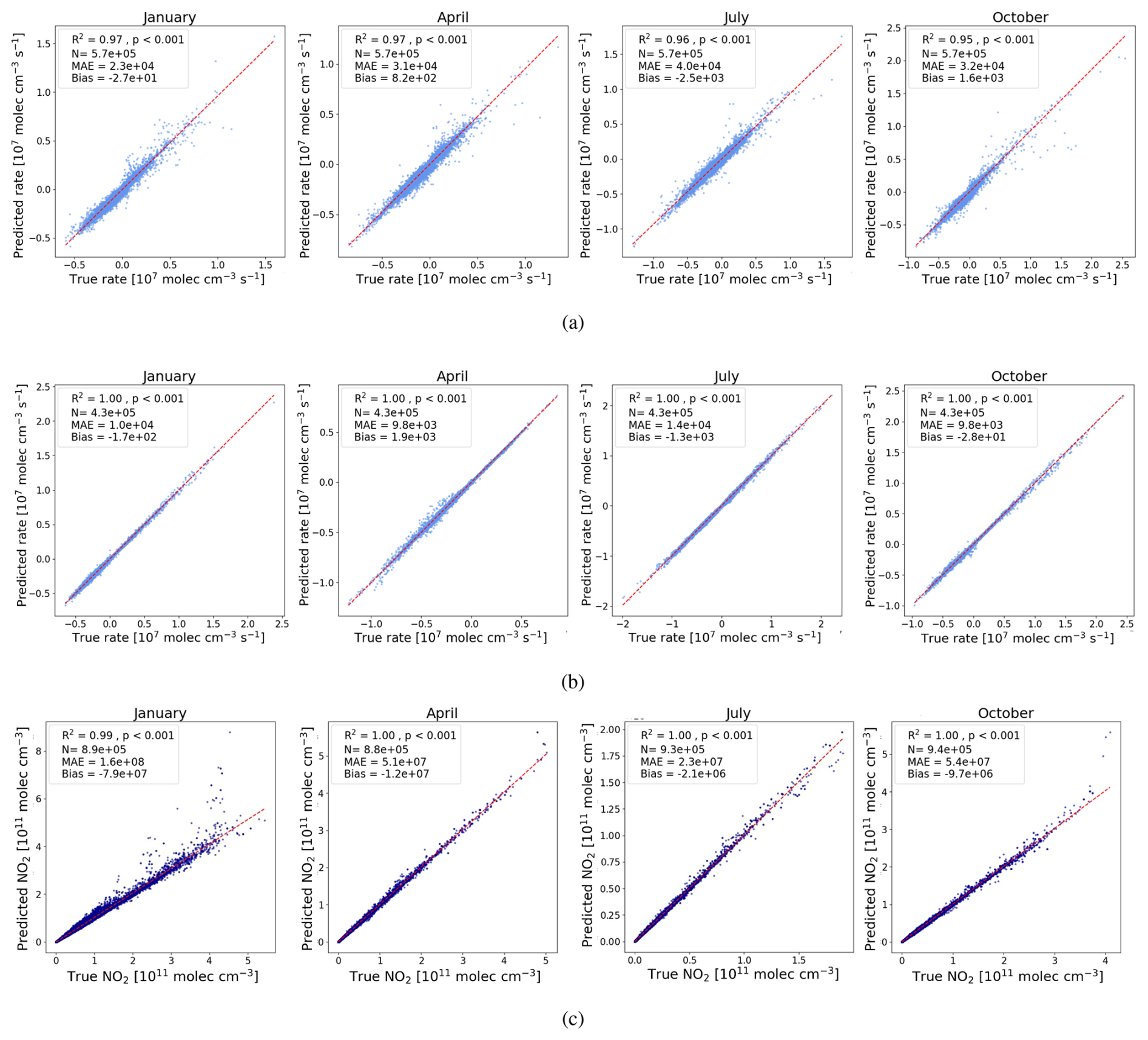
Figure 3 Actual versus predicted scatter plots for models tested on simulations with unseen emission perturbations. (a) The random forest regression model for predicting the NO_x chemistry rate, (b) the constant lifetime scaling for reconstructing the NO_x chemistry rate using an unperturbed chemistry dataset, (c) the reconstruction of NO₂ from NO_x using the random forest regression model for predicting the NO₂ : NO ratio.

We also tested our regression-based atmospheric chemistry model with model data from 2021 (Fig. A6). As expected, the regression model performance has less skill in reproducing data that has not been used for training. In this case, the MAE values are higher by a factor of 1.3–1.8 compared with the overall performance comparison shown in Fig. 4). Nevertheless, the model still shows substantial skill despite substantial differences in anthropogenic emissions between 2019 and 2021 due to COVID-19. Specifically, NO_x emissions were found to decrease by 18 %–24 % during lockdown periods (Miyazaki et al., 2021) leading to a mean observed reduction in NO₂ of 29 % (Cooper et al., 2022).

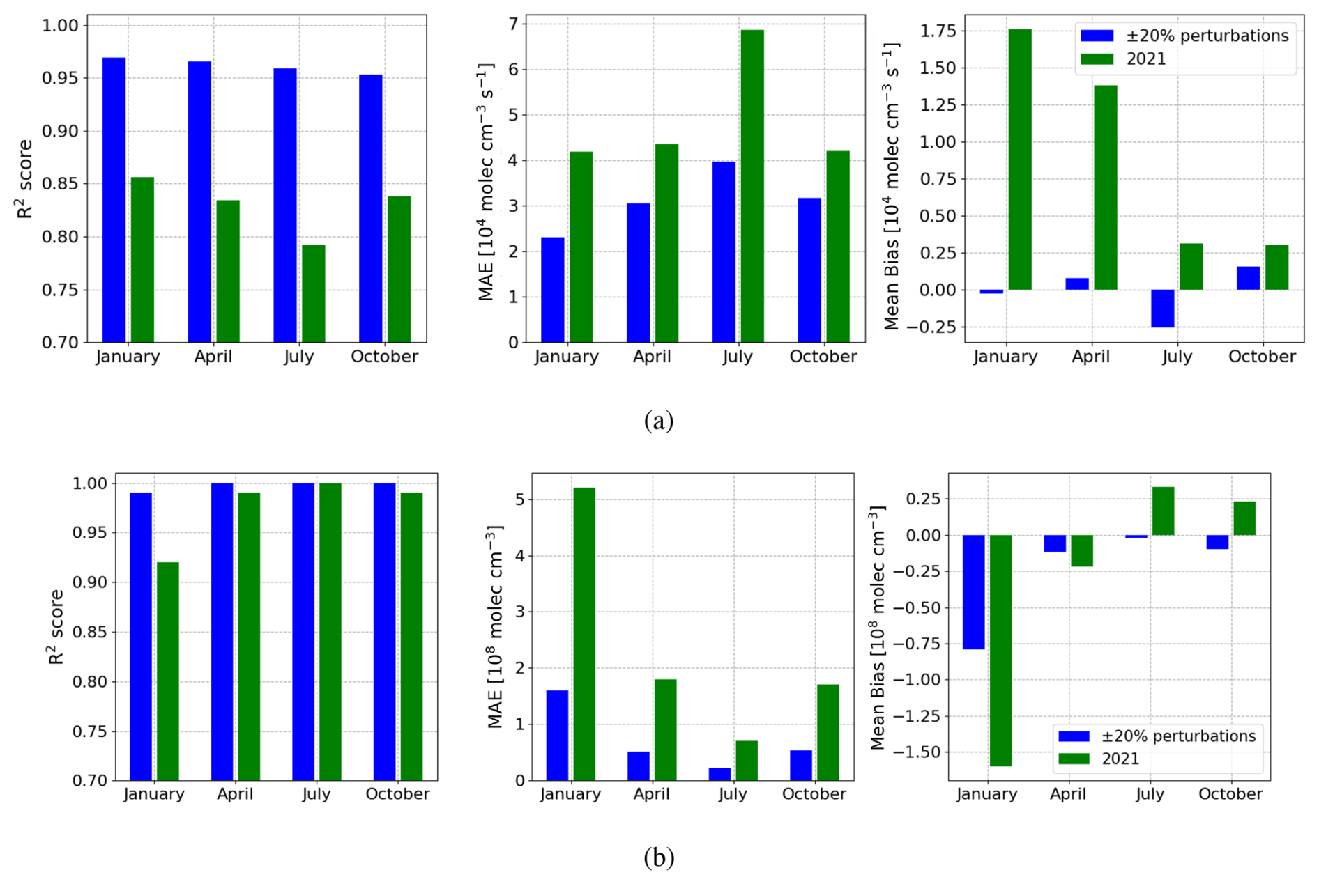
Figure 4 Regression model prediction performance compared when tested on a 20 % perturbed model run for 2019 and an unseen year, 2021. Panel (a) shows the NO_x chemistry regression model performance comparisons and panel (b) shows the NO₂ prediction performance using the NO₂ : NO regression model.

3.1.2 NO_x chemistry prediction using constant lifetime scaling

Figure 3b shows results from using our alternative atmospheric chemistry regression NO_x model that employs a constant atmospheric lifetime scaling approach (Eq. 4). The resulting model performance is a significant improvement above the other regression model for all 4 study months. Using our scaling approach, we found consistent values of R² = 1.0 and MAE values that are approximately 2–3 times smaller than the other regression model. As with the other regression model, the size of the error is scaled by the seasonal changes in chemistry rates.

While this approach shows extremely encouraging abilities to determine NO_x chemistry rates, its effectiveness relies on having a full-chemistry model run available for at least one set of emission inputs. Consequently, this approach is particularly useful for emission perturbation studies, for which numerous emission distribution scenarios might be needed for model inversion work. In this case, the full-chemistry model would only need to be run once for the given time period of interest. However, we cannot predict the NO_x chemistry using this method for a previously unmodelled meterological period.

3.1.3 NO₂ : NO ratio regression model

We find the random forest regression model to predict NO₂ : NO ratios also demonstrates significant performance. The predicted ratio is used to convert NO_x concentrations to NO₂ concentrations (Eq. 2). Figure 3c shows that the regression model can reproduce “true” NO₂ values from the full-chemistry of the GEOS-Chem model, with values of R² of 1.0; the exception is January when R² = 0.99.

Generally, the model performance is better during summer months and worse in winter months, with MAE values an order of magnitude smaller in July compared to January. This is partly due to NO₂ concentrations increasing during colder months due to increased combustion and longer nights, and because we find that NO₂ : NO ratios become increasingly hard to determine at higher solar zenith angles, typically experienced over Europe during daytime through winter months. We also examine the performance of this regression model using data from the unseen year 2021. As with the atmospheric chemistry regression model, described above, the performance was good but worse than for 2019 in which data was used to train the model. The MAE increased by a factor of 3.25, 3.52, 3.04, and 3.14 for January, April, July, and October respectively. We found the R² performance reduced most for January from 0.99 to 0.92, During April and October R² reduced from 1.0 to 0.99, while R² = 1.0 was maintained in July.

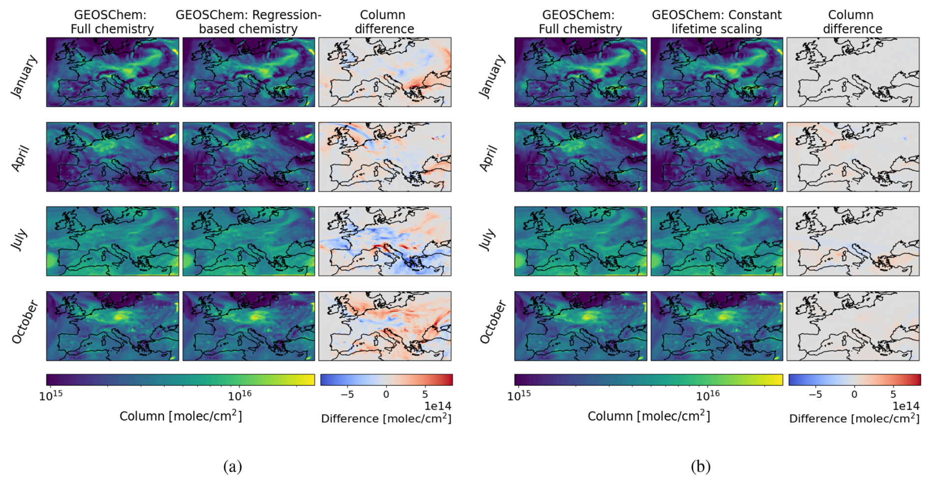
Figure 5 The modelled NO_x columns sampled at 12:00 UTC after a 10 d model run with ±20 % emission perturbations. NO_x columns are compared for the GEOS-Chem full-chemistry model and (a) NO_x columns are simulated using the regression-based chemistry method and (b) using the constant lifetime scaling method.

3.2 NO_x atmospheric modelling

Figure 5 shows the NO_x column reconstruction for the two regression models used to describe the NO_x chemistry rates from the full-chemistry version of the GEOS-Chem model. From a visual inspection, there are no obvious differences in the spatial distribution of the NO_x columns reconstructed using both the regression-based chemistry model and the constant lifetime scaling model. However, when mapping the differences, there are areas of deviation from the full-chemistry model. Broadly, this deviation is significantly smaller when we use the scaling-based model compared to the regression-based. In addition, the error accumulation in January is notably smaller than in other months.

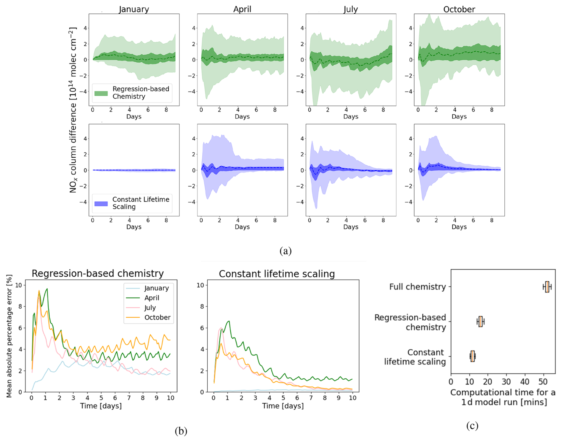
Figure 6 Comparison of the temporal variation in NO_x column reconstruction for the regression-based and scaling-based model. (a) The median (dashed line), IQR (light-shaded region) and range (dark-shaded region) of the NO_x column reconstruction error over the 10 d runs. (b) The mean absolute percentage error over the 10 d runs. (c) Shows the reduction in computational time when modelling atmospheric NO_x using each of our chemistry prediction methods compared to running with the full-chemistry model.

Figure 6 shows the temporal variation in the reconstruction error. The range, IQR, and median values are shown in Fig. 6a and the mean absolute percentage error (MAPE) is shown in Fig. 6b. For the regression-based chemistry method the range in deviation peaks at up to 3 × 10¹⁴ molec. cm⁻² in January, 5 × 10¹⁴ molec. cm⁻² in April and 6 × 10¹⁴ molec. cm⁻² in July and October. This is reflected in maximum MAPE values of 2.8 %, 9.7 %, 8.9 %, and 9.3 % for the 4 months, respectively. On the whole, the MAPE reduces through time, with final deviation values of 1.7 %, 3.4 %, 2.0 %, and 4.8 % after the full 10 d run.

Reconstruction errors for the constant lifetime scaling model show much smaller errors, particularly in January, with MAPE < 0.2 % throughout the 10 d run. This is driven by the smaller impact that emission perturbations have on the NO_x chemistry in January as shown by Fig. A5. In particular, the lifetime of NO_x is relatively unchanged between the unperturbed and perturbed model runs. This reduced impact in January is likely due to the slower rate of photochemical reactions in the winter months and increased atmospheric stability at lower temperatures. The other months do see a more prominent deviation of up to a maximum of 4 × 10¹⁴ molec. cm⁻², with peak MAPE values of 6.6 %, 5.7 %, and 4.5 %, for April, July, and October, respectively. As with the regression-based model outputs, here the MAPE also generally decreases through time with final deviation values of 0.1 %, 1.1 %, 0.2 %, and 0.3 % for each month, respectively. Interestingly, while the range and IQR are relatively stable throughout the run when using the regression-based reconstruction, these quantities decrease considerably with time when we use the scaling-based reconstruction.

The reconstruction error has a small diurnal cycle, peaking in the morning and to a lesser extent in the evening, reflecting the diurnal cycle of NO_x chemistry (Fig. A1). Overall the absolute model error for both the regression-based and scaling-based methods peaks after the first day and then gradually reduce, plateauing by ≃day 6. This early peak in error followed by a reduction and eventual plateau is likely due to compensating errors, where the regression model's over- and under-predictions balance each other out over time, leading to a stabilisation of the overall error. It is encouraging that there is no accumulation of error through time, suggesting this approach would be suitable for studies longer than for 10 d. It is clear that the optimal reconstruction performance is found when using the scaling-based method, but as we already note there are limitations to this method. The regression-based approach still provides excellent reconstruction performance for our purposes.

Figure 7 (a) The modelled NO_x columns sampled at 12:00 UTC after a 10 d model run in 2021 using the regression models trained on 2019 compared with full-chemistry. (b) The mean absolute percentage error for the 10 d runs.

To evaluate the performance of the regression-based chemistry modelling approach with regression models trained on a different meteorological time period, the same models were applied to simulate atmospheric NO_x over Europe for 2021. Figure 7a shows the reconstructed NO_x columns after a 10 d model run. As expected, the reconstruction performance is clearly worse than when the regression-based chemistry is just applied in 2019 with emission perturbations (Fig. 5a). However, from a visual inspection, there are no obvious changes to the spatial distribution of the NO_x columns reconstructed using regression-based chemistry in comparison to the full-chemistry model output. Additionally, the temporal variation in error is shown through plots of the MAPE (Fig. 7b). We see maximum MAPE values of 11.0 %, 10.0 %, 16.7 %, and for January, April, July, and October 2021 respectively. For all months this is an increase in the maximum deviation observed when applying this methodology to a perturbed 2019 run. Overall, this is reflective of the reduction in prediction power of the regression models when we apply to 2021, which has unseen meteorology. Overall, the same pattern of the absolute error gradually reducing and plateauing by ≃ day 6 is also observed here. However, the diurnal cycle of variation in the reconstruction error is more pronounced in the 2021 case, likely due to the fact that the regression model is worse performing during the night for unseen meteorology. The error tends to reduce dramatically towards the middle of the day, which is helpful if we consider the application of model comparison with satellite data such as a TROPOMI, which has a 13:30 overpass time.

Substantial computational time is saved when we employ these regression methods to model atmospheric NO_x. Figure 6c shows the time taken for each model to perform a 1 d model run. This was calculated as the mean average for the model to run for a single day out of the 10 d run for each of the 4 months, repeated for 3 model runs. Clearly, the full-chemistry model takes the longest, with a mean of 52 min per day for our nested model over Europe. The regression-based chemistry model is significantly faster with a mean of 16 min (3.25 times improvement), while the constant lifetime scaling method is even faster, with a mean of 12 min (4.3 times improvement). It is important to note that the model run times reported here are subject to variability due to fluctuations in the relative loading experienced by the computer system used.

3.3 NO₂ column reconstruction

Finally, we assess the capability of our NO₂ : NO regression model, convolved with TROPOMI instrument averaging kernels, to reproduce observation column distributions of NO₂ from TROPOMI. The absolute differences in NO₂ columns between GEOS-Chem full-chemistry and the GEOS-Chem regression-based and scaling-based models are compared to the absolute difference in TROPOMI NO₂ and GEOS-Chem full-chemistry, as well as to the magnitude of the TROPOMI NO₂ column precision data. This is presented in Fig. 8a, compared for 8 d in January, April, July, and October. We apply the regression-based method to a 2019 perturbed model run, and to a 2021 model run.

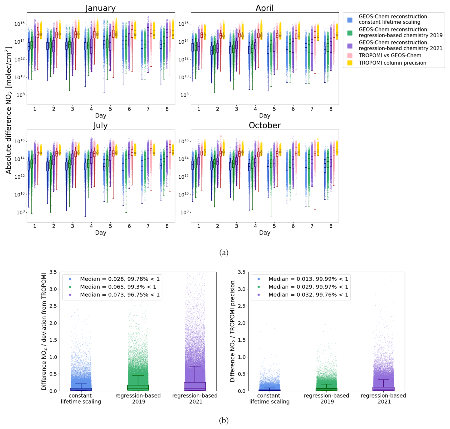
Figure 8 (a) The absolute difference in NO₂ between GEOS-Chem full-chemistry and the constant lifetime scaling based model (blue); the regression-based chemistry model applied to a 2019 perturbed run (green) and applied to a 2021 run (purple); deviation from the observed NO₂ TROPOMI columns (red); as well as the TROPOMI NO₂ tropospheric column precision values (yellow). (b) The normalised NO₂ differences are calculated by normalising the reconstructed model deviation by the absolute deviation between GEOS-Chem and TROPOMI, as well as by the TROPOMI column precision values. For the different model reconstructions, the NO₂ deviation is consistently less than the corresponding TROPOMI precision value in more than 99.5 % datapoints.

We find comparable NO₂ reconstruction errors for the 4 months we study. Earlier, with the NO_x reconstruction, we found that the error was smaller for January than the other months (Fig. 3a and b), however, the higher error from the January NO₂ : NO regression model (Fig. 3c) offsets this advantage, ultimately bringing the overall reconstruction error for all months to a comparable level. We observe comparable magnitudes of reconstruction error when we compare our NO₂ reconstructions based on the scaling-based and regression-based methods applied to the 2019 model run. However, the reconstruction error tends to be consistently larger when we apply our regression-based method to the year 2021. This is particularly notable in January and July, which can be attributed to the greatest deterioration in NO_x chemistry regression performance in July 2021, and the greatest deterioration in the NO₂ prediction performance in January 2021 (see Fig. 4).

When we compare the difference between GEOS-Chem and TROPOMI NO₂ columns, we find that the NO₂ reconstruction errors are much smaller and much smaller than the estimated precision values for the data. This is the case for the scaling-based approach and the regression-based approach applied to both 2019 and 2021. This provides confidence that our model reconstruction performance is robust enough for use in inversion work, even in the case of using regression models that have been trained on unseen meteorological periods. See Appendix B for a more detailed analysis on the difference between modelled column NO₂ and observed TROPOMI data.

Figure 8b, shows that the median NO₂ column model reconstruction errors are 2.8 % of the actual deviation from TROPOMI in the scaling-based approach, compared to 6.5 % and 7.3 % in the regression-based approach for 2019 and 2021, respectively. Similarly, these construction errors represent a median value of 1.3 % of the TROPOMI precision value for the scaling-based approach, compared to 2.9 % and 3.2 % for the regression-based approach for 2019 and 2021, respectively. Across all reconstructed data points, we found that over 99.9 % of the data had reconstruction errors smaller than the corresponding TROPOMI column precision for both reconstruction methods in 2019. For the regression-based method applied in 2021, this was true for over 99.7 % of the data.

4 Concluding remarks

We have demonstrated that the NO_x chemistry rates and NO₂ : NO ratio described by a leading 3-D atmospheric chemistry model can be reproduced using random forest-based regression models using NO_x concentrations, the spatial location, and meteorological variables as input parameters. The models perform successfully on perturbed testing data through all months of 2019 with R²>0.95 for predicting NO_x chemistry rates and R²>0.99 for predicting the corresponding NO₂ : NO concentration ratios. We also show that these models maintain their prediction capability when tested on model outputs from an unseen year (2021) with contrasting environment conditions.

We have also demonstrated that the atmospheric lifetime of NO_x is stable against varying emissions, particularly in winter months. From this, we have demonstrated that it is also possible to predict updated NO_x chemistry rates of change as a result of emission perturbations, with knowledge of NO_x chemistry from an initial unperturbed model run. This scaling-based approach has impressive prediction performance with R² = 1.0.

We have developed two viable methodologies to model atmospheric NO_x in a more computationally efficient way than using the GEOS-Chem 3-D model. The regression-based chemistry method has the advantage of not requiring prior knowledge of the NO_x lifetimes for a baseline model run, and reduces the computational time by a factor of 3.25. The lifetime scaling-based approach reduces the model run time slightly further by a factor of 4.3, but a baseline full-chemistry model run is required. This scaling-based approach has smaller model reconstruction errors, but generally both approaches have reconstruction errors smaller than the TROPOMI precision values for over 99.9 % of the reconstructed data (399 502 points).

Our study provides confidence in random forest models being used to describe NO_x chemistry to a sufficient accuracy for them to play an important role in inversion methods. Previous work has already found that NO₂ can be used to help constrain ffCO₂ (Berezin et al., 2013; Lopez et al., 2013; Goldberg et al., 2019; Super et al., 2020), and this work develops a new methodology to more efficiently infer NO₂ column enhancements from changes to NO_x emission inputs. The methodologies developed here will be used within a joint NO_x : CO₂ model inversion to constrain geographically resolved ffCO₂. This will be explored using an ensemble Kalman filter within the GEOS-Chem model framework, as well as within the Integrated Forecasting System (IFS) using an incremental 4D-Var algorithm (Inness et al., 2013). Results from our study are particularly timely with the launch in the next few years of the Copernicus Anthropogenic Carbon Dioxide Monitoring constellation (CO2M) that include column measurements of CO₂ and NO₂. Overall this work will support the development and employment of European CO₂ measurement, reporting and verification systems.

Appendix A

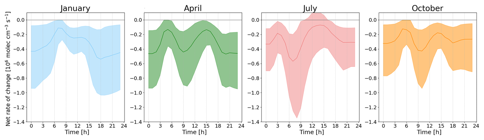
Figure A1 Diurnal cycle of NO_x chemistry for 4 months of the year. Median and interquartile range net rates of change at the surface of the atmosphere averaged across the European domain.

Figure A2 (a) Feature selection results for the rate prediction models, obtained using a forward selection wrapper method. Plotted are the coefficient of determination (R²) and mean absolute error (MAE) as functions of the number of features included, for each of the four seasonal models (January, April, July, October). (b) Same as (a), but for the partitioning ratio prediction models. (c) Feature importance distributions for each of the four monthly models, showing the relative contributions of each predictor variable to the rate prediction models (using nine features) and the partitioning ratio prediction models (using eight features). (d) Change in MAE resulting from the removal of each of the 14 features in turn, demonstrating the individual impact of each feature on model performance and highlighting the importance of specific predictors for accurate rate and ratio estimates.

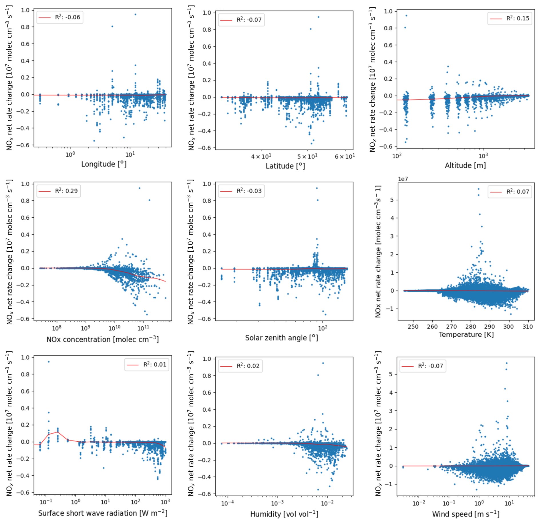
Figure A3 Individual relationships between the nine regression input parameters and the NO_x net rate of change. A LOWESS fit (red line) illustrates smoothed trends in the data, with R² values reported for each fit. Among the parameters, NO_x concentration, altitude, and temperature exhibit noticeable trends with chemistry rates, while the remaining parameters show little to no clear trends individually.

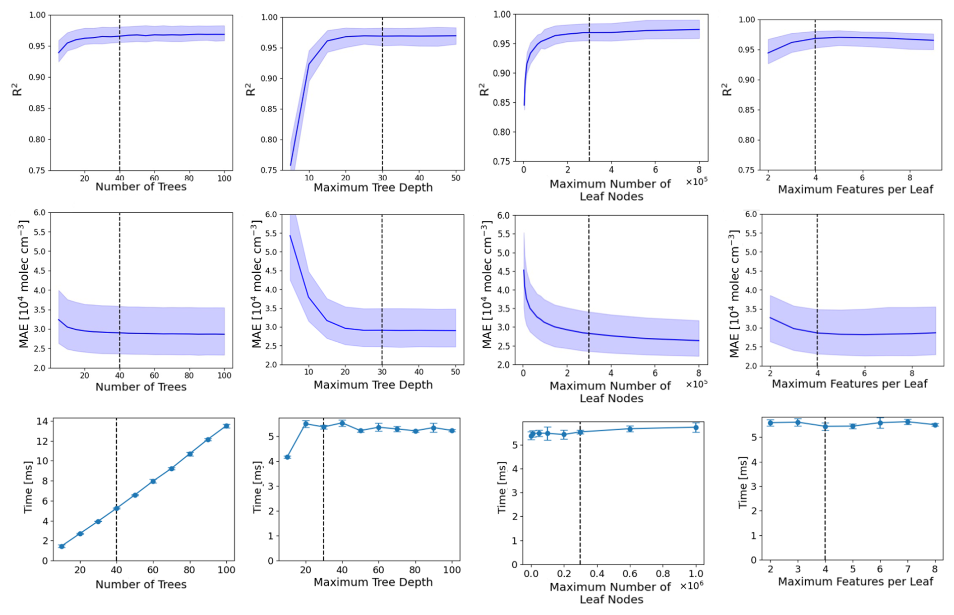
Figure A4 Impact of hyperparameter changes on random forest regression model performance for predicting NO_x chemistry rates. Plots show the effect of varying the number of trees, maximum tree depth, maximum leaf nodes, and maximum features per decision on mean R², MAE, and prediction time (shaded regions represent performance ranges across monthly models). Increased algorithm complexity improves R² and reduces MAE but increases prediction time. Optimal hyperparameters – 40 trees, depth of 30, 300 000 leaf nodes, and 4 features per decision – achieve balanced performance with a prediction time of 6 ms.

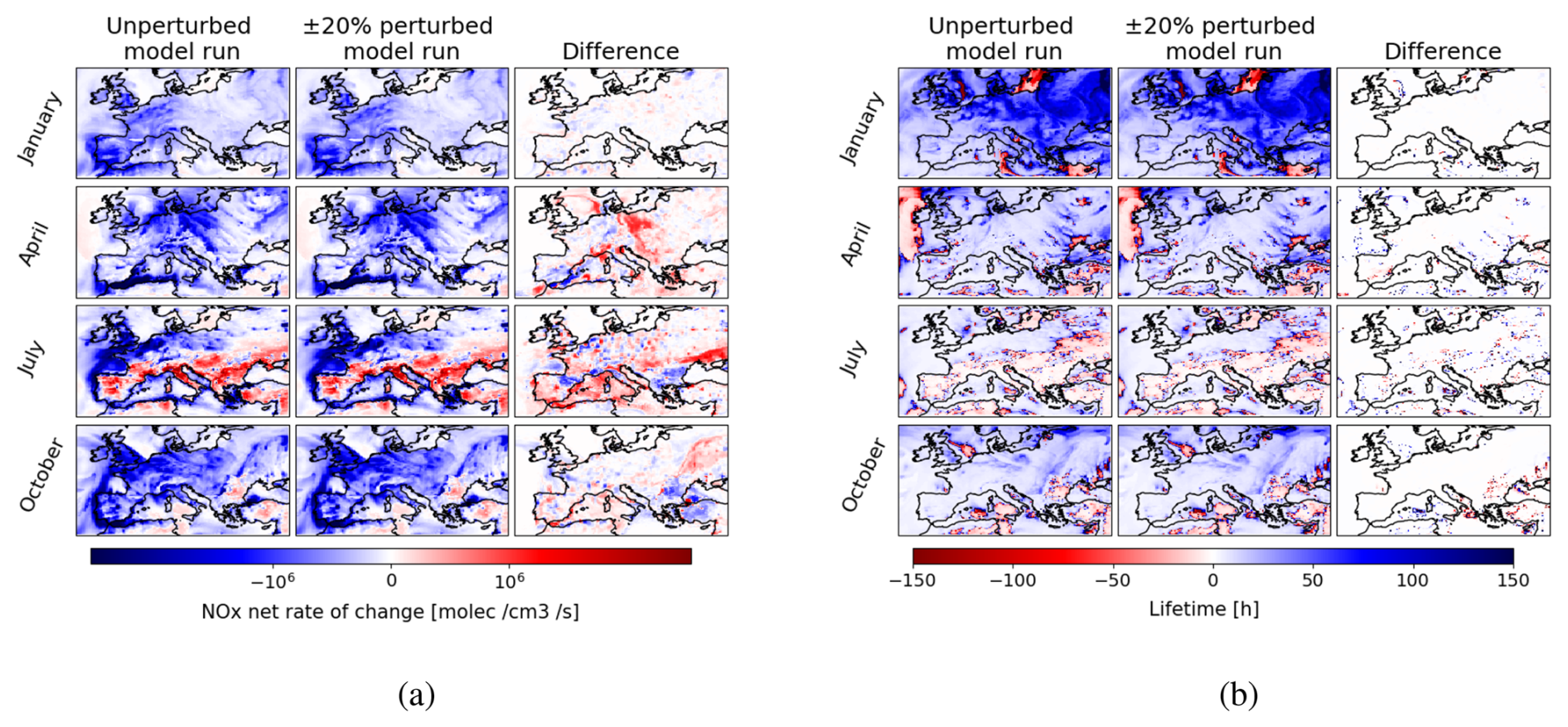
Figure A5 The spatial distribution of the impact of ±20 % emission perturbations on (a) the NO_x net rate of change, and (b) the atmospheric lifetime of NO_x. Overall, it is clear that the impact on the atmospheric lifetime is much smaller, due to its independence from the NO_x species concentration. Note that a negative lifetime of NO_x arises in areas where we have a net chemical production of NO_x.

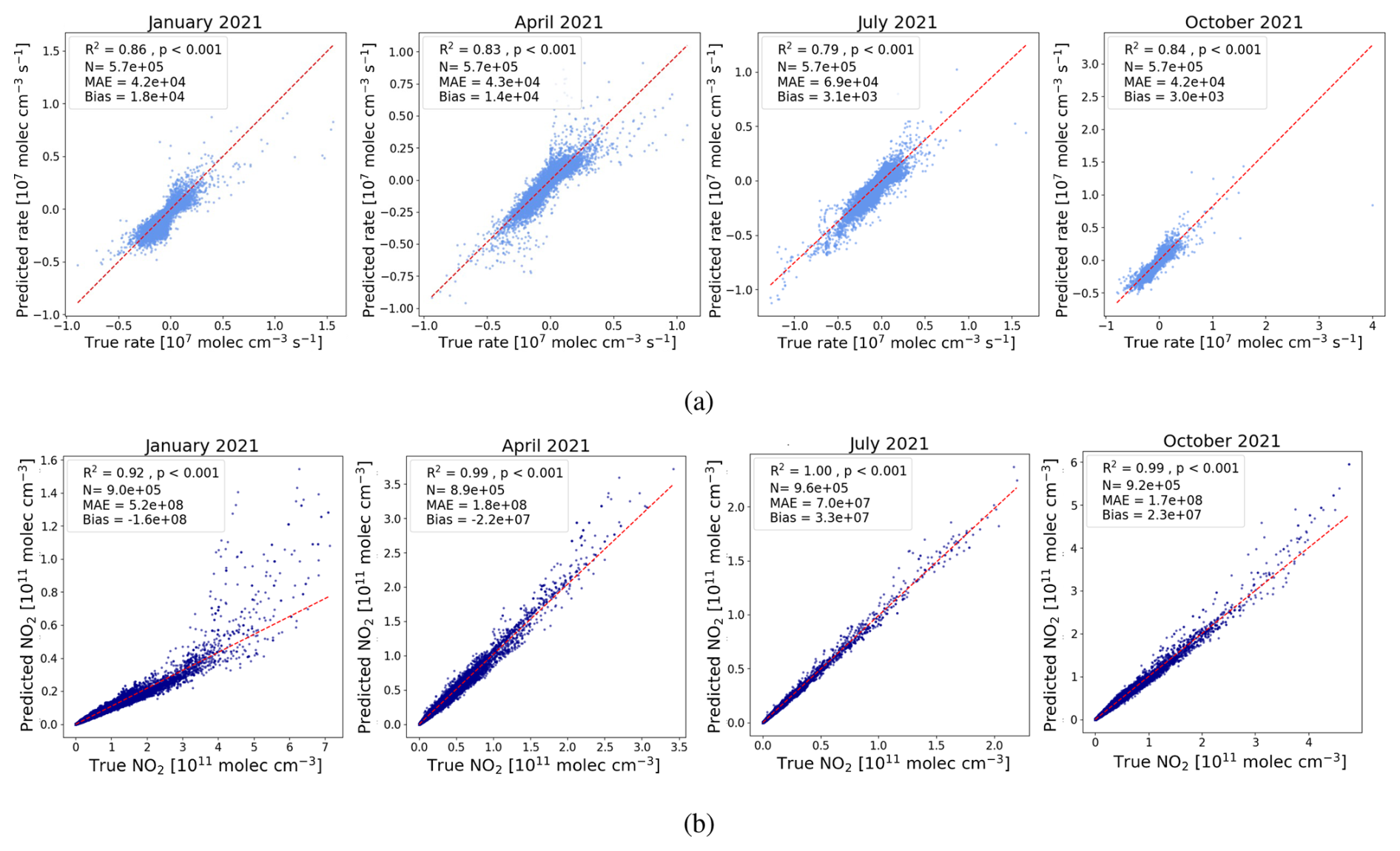
Figure A6 Testing the regression models on 2021. (a) The random forest regression model for predicting the NO_x chemistry rate, (b) the reconstruction of NO₂ from NO_x using the random forest regression model for predicting the NO₂ : NO ratio.

Appendix B: Comparison with TROPOMI

The NO₂ columns modelled by GEOS-Chem was compared directly with the TROPOMI data for assessment of agreement. Scatter plots between the two are shown in Fig. B1, where we found significant Pearson correlations (p<0.001) in all months. In January we observe a general positive bias, where the model is overestimating NO₂, while in July and October, a negative bias is seen.

The spatial distribution of the deviation between GEOS-Chem and TROPOMI is shown in Fig. B2. While there are clear areas of difference, it is notable that the general regions where we observe elevated levels of NO₂ are in alignment. In general, the spatial distribution of high-emission regions throughout Europe is fairly well understood. However, there is likely some error on the magnitudes of the emissions in the inventories used. This is likely to explain the majority of the areas of large bias between the model and the observations. However, it must be noted that other sources of error are present, which include model errors in transport processes, potential inaccuracies in the model meteorology used, errors in parameterising deposition processes, and the limiting factor of the model spatial resolution. Furthermore, there is also error on the TROPOMI measurements (largely characterised by the TROPOMI column precision value) including from instrument noise, cloud and aerosol interference, and vertical profile and sensitivity assumptions. Looking to Fig. 8 it is clear that there are many regions where the error between the model and observations is significantly smaller than the satellite precision, and for such areas the contribution of NO_x emissions is likely to be accurate.

On the whole, it is promising to the performance of the model that there is a general correlation of agreement between the model and satellite data. However, there is room for improvement in model agreement, and model inversions would be one approach to achieve this.

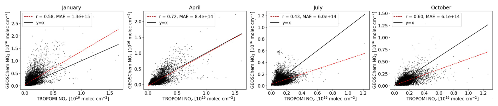
Figure B1 Correlation between modelled GEOS-Chem NO₂ columns and observed TROPOMI NO₂ for the 4 months of interest. The Pearson rank and mean absolute area are shown in the legend. The best-fit line (red-dashed) can be compared to the y=x line (black).

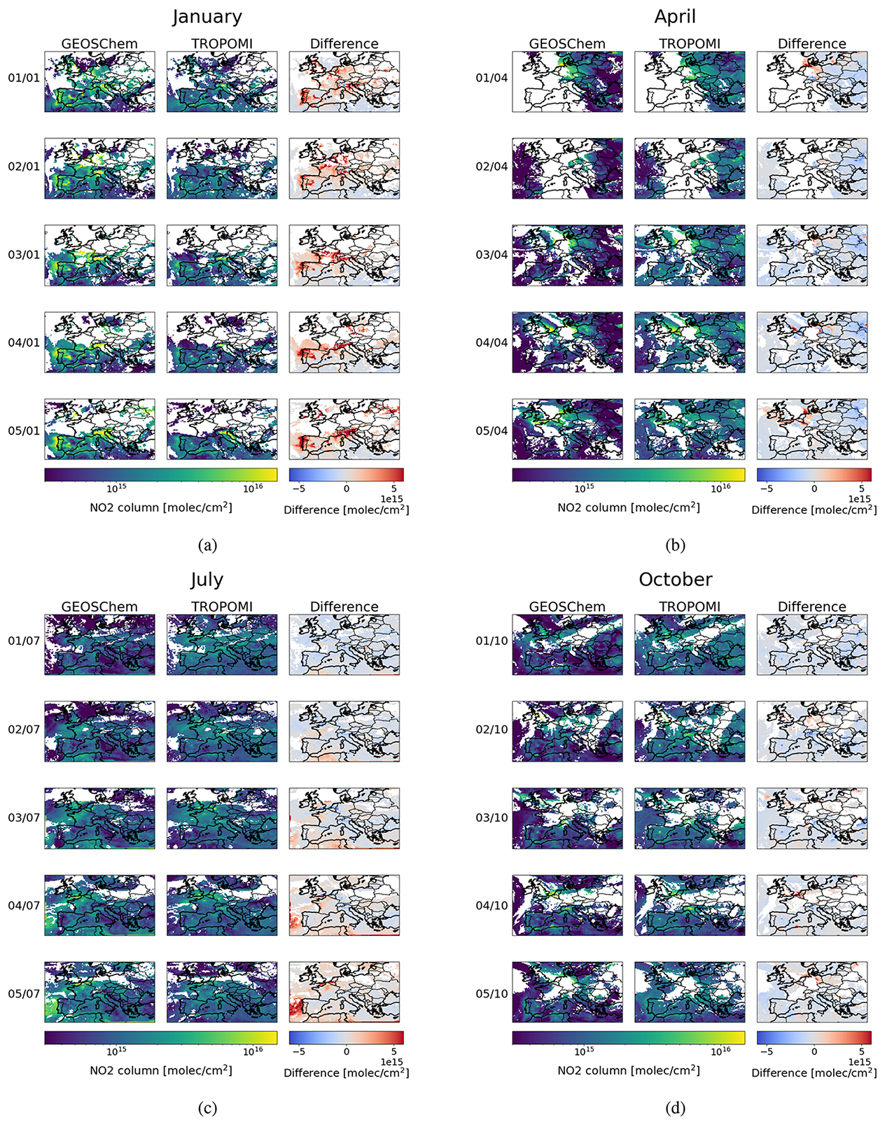
Figure B2 Comparison between GEOS-Chem and TROPOMI for 5 d in January, April, July, and October.