the Creative Commons Attribution 4.0 License.
the Creative Commons Attribution 4.0 License.
 | 04 Feb 2025
Biomass burning emission analysis based on MODIS aerosol optical depth and AeroCom multi-model simulations: implications for model constraints and emission inventories
Mariya Petrenko
Mian Chin
Susanne E. Bauer
Tommi Bergman
Huisheng Bian
Gabriele Curci
Ben Johnson
Johannes W. Kaiser
Zak Kipling
Harri Kokkola
Xiaohong Liu
Keren Mezuman
Tero Mielonen
Gunnar Myhre
Xiaohua Pan
Anna Protonotariou
Samuel Remy
Ragnhild Bieltvedt Skeie
Philip Stier
Toshihiko Takemura
Kostas Tsigaridis
Hailong Wang
Duncan Watson-Parris
Kai Zhang
We assessed the biomass burning (BB) smoke aerosol optical depth (AOD) simulations of 11 global models that participated in the AeroCom phase III BB emission experiment. By comparing multi-model simulations and satellite observations in the vicinity of fires over 13 regions globally, we (1) assess model-simulated BB AOD performance as an indication of smoke source–strength, (2) identify regions where the common emission dataset used by the models might underestimate or overestimate smoke sources, and (3) assess model diversity and identify underlying causes as much as possible. Using satellite-derived AOD snapshots to constrain source strength works best where BB smoke from active sources dominates background non-BB aerosol, such as in boreal forest regions and over South America and southern hemispheric Africa. The comparison is inconclusive where the total AOD is low, as in many agricultural burning areas, and where the background is high, such as parts of India and China. Many inter-model BB AOD differences can be traced to differences in values for the mass ratio of organic aerosol to organic carbon, the BB aerosol mass extinction efficiency, and the aerosol loss rate from each model. The results point to a need for increased numbers of available BB cases for study in some regions and especially to a need for more extensive regional-to-global-scale measurements of aerosol loss rates and of detailed particle microphysical and optical properties; this would both better constrain models and help distinguish BB from other aerosol types in satellite retrievals. More generally, there is the need for additional efforts at constraining aerosol source strength and other model attributes with multi-platform observations.
- Article
(7075 KB) - Full-text XML
-
Supplement
(742 KB) - BibTeX
- EndNote


Aerosol particles emitted from biomass burning (BB) play a significant role in both regional climate and air quality and, in aggregate, can contribute significantly to direct and indirect aerosol climate forcing (e.g., Andreae et al., 2004; Bowman et al., 2009; Gadhavi and Jayaraman, 2010; Ichoku et al., 2012; Lelieveld et al., 2015; Lu et al., 2018; Randerson et al., 2006; Solomos et al., 2015). One of the challenges of representing BB smoke in models that assess their environmental impacts is adequately characterizing the strength of BB sources.
Several approaches have been taken to estimate smoke source strength. A widely used set of methods involves calculating the product of burned area, available fuel load, combustion completeness, and emission factors of primary aerosols and precursor gases (Seiler and Crutzen, 1980), where the latter three quantities are determined, to the extent possible, from field observations. Burned area is derived from reflectance changes in satellite imagery (e.g., Chen et al., 2023; Giglio et al., 2006a; Roy et al., 2008; Soja et al., 2004; Vermote et al., 2009; Wiedinmyer et al., 2011, 2023) or deduced, with some assumptions, from space-based 4 µ brightness temperature anomaly (designated fire radiative power or FRP) measurements (Chen et al., 2023; Randerson et al., 2012; van der Werf et al., 2006). Other approaches exploit correlations between FRP and combustion rate (Kaiser et al., 2009; Wooster et al., 2005). The active fire (FRP)-based methods are generally more sensitive to small fires than those relying on burned area estimates; however, FRP is more affected by observational gaps due to sampling frequency limitations and cloud cover, whereas burned area can be assessed for some time after active burning has ceased (e.g., Randerson et al., 2012).
Observations of FRP combined with the aerosol optical depth (AOD) of the smoke plume itself and/or the difference between the 4 and 11 µ brightness temperatures, all obtained from the NASA Earth Observing System's MODerate resolution Imaging Spectroradiometer (MODIS) instruments, have also been used directly to estimate smoke emissions (Ichoku and Ellison, 2014; Ichoku and Kaufman, 2005; Kaiser et al., 2012; Konovalov et al., 2014; Sofiev et al., 2009; Wooster et al., 2005). One implementation of this approach (Ichoku and Ellison, 2014) uses the plume AOD and area divided by the advection time, estimated from the apparent length of the plume in the MODIS imagery and a wind speed obtained from a reanalysis product, and correlates this quantity with the FRP for multiple cases to derive ecosystem-specific coefficients, which, when multiplied by the observed FRP for individual fires, yield a smoke mass emission estimate.
Inverse modeling has also been applied in efforts to characterize aerosol source strength from large-scale maps of AOD (e.g., Chen et al., 2019; Dubovik et al., 2008; Vermote et al., 2009). With this approach, a version of an aerosol transport model is effectively run in reverse, initialized with a regional or global AOD distribution, to trace back to the locations and strengths of the aerosol sources. However, this approach requires all other aspects, e.g., transport, removal, chemical transformation, source location, and non-BB aerosols, and the assumptions made to constrain aerosol properties and processes to be adequately represented in the model.
Bottom-up inventories are derived from laboriously collected information about primary and secondary aerosol sources, both anthropogenic and natural, to estimate the resulting aerosol accumulation in the atmosphere (e.g., Anderson et al., 2024; Chen et al., 2019, 2023; Liousse et al., 2010; Petrenko et al., 2012; Schultz et al., 2008; Seiler and Crutzen, 1980; van der Werf et al., 2010, 2017; Wiedinmyer et al., 2023). This approach has been an essential tool for approximating aerosol loading for times prior to global satellite observations and continues to be a key resource for estimating regional aerosol amounts and types, but it suffers from limited knowledge about source properties, as well as unknown sources that would be missing altogether.
Not surprisingly, there are significant discrepancies among the different estimates of BB aerosol source strength (e.g., Carter et al., 2020; Pan et al., 2020; Petrenko et al., 2012, henceforth P2012). In an effort to bring additional satellite-based constraints to bear on smoke source–strength estimates globally, P2012 adopted a forward-modeling approach that made explicit use of known smoke source locations and compared model-derived estimates of aerosol loading for varying aerosol source strength with satellite-derived AOD rather than using the top-of-atmosphere brightness temperature itself to characterize smoke source strength. Region-specific summaries of the relationships between smoke emission rates used in the model and MODIS-retrieved snapshots of AOD for individual plumes were provided. In particular, in the P2012 study, the GOCART model (Chin et al., 2002, 2014) was initialized with varying BB sources, as specified by a number of widely used smoke source emission inventories, including the Global Fire Emission Database version 3 (GFED3) (Randerson et al., 2012, 2013; van der Werf et al., 2010). The model was sampled at the time closest to that of the satellite overpass, and the near-source AOD of the model was compared with that derived from coincident MODIS observations. One key observation from this study is that the model-simulated AOD bias within a given geographic region is systematic, such that the model overestimated, underestimated, or approximately agreed with the observed AOD snapshots for nearly all plume cases within that region. This indicated that it might be possible to apply region- and/or biome-specific adjustment factors to the emission inventories to bring the model into agreement with the observations.
Petrenko et al. (2017; henceforth P2017) greatly expanded the database of smoke cases in P2012 and refined the model–observation comparisons (1) using scaled AOD reanalysis values from the Modern-Era Reanalysis for Research and Applications (MERRAero) to fill AOD in those parts of plumes that are too optically thick to use to derive AOD from MODIS observations and in areas obscured by clouds, (2) distinguishing to the extent possible the emitted BB aerosol from background aerosol generated by other sources, and (3) assessing qualitatively the effect of small fires based on emissions from the GFED4.1s database (Giglio et al., 2013; Randerson et al., 2017, 2018; van der Werf et al., 2017) to account for fires that are too small to be detected by the standard satellite-based methods used for GFED3. This analysis showed that the overall approach works best when the total AOD and the BB fraction of the total AOD are high, which occurs primarily for evergreen or deciduous forest fires. Ambiguities arise when either the background AOD is comparable to or larger than the BB contribution, generally in heavily polluted regions such as northern India and eastern China, or when the total AOD is low, which can occur in regions of sparse vegetation or agricultural burning.
The P2012 and P2017 studies looked only at results from the GOCART model, which provided a consistent set of results that were relatively straightforward to interpret in terms of emission source strength. However, those studies did not address the uncertainties associated with a range of underlying model assumptions that are not constrained by the choice of BB emission source strength alone. The current study expands upon this earlier work by examining the behavior of 11 global models that are part of the AeroCom community. The results highlight some of the leading model assumptions and not well-constrained by measurements that affect model-simulated AOD, even when the emission strength is specified.
AeroCom is an open international initiative providing a platform for multi-model intercomparison and comparisons between observations and models (https://aerocom.met.no/, last access: 22 January 2025). AeroCom has a long history of performing multi-model experiments in which certain factors are controlled among the model runs, and comparative analysis yields insights into the impact of different model assumptions and parameterizations (e.g., Bian et al., 2017; Curci et al., 2015; Gliß et al., 2021; Huneeus et al., 2011; Kim et al., 2019; Kinne et al., 2006; Textor et al., 2006; Tsigaridis et al., 2014; Zhong et al., 2022). These efforts have produced a great many insights into the factors affecting model performance and have made it possible to isolate model-specific factors from issues associated with external constraints. Following this tradition, and as part of the larger AeroCom phase III experiments, the biomass burning experiment aims to assess the emission source strength (BBESS) and injection heights (BBEIHs) that are used in models in the context of global satellite-derived constraints and to identify any model-related issues that arise from the comparisons.
The current paper reports the results of the AeroCom BBESS experiment for which the same BB emission inventory from the Global Fire Emission Dataset version 3.1 (GFED3.1) is used in all participating models. The model-simulated results are evaluated region by region with the MODIS smoke plume reference database developed in P2012 and P2017 (the data set of study fire cases is contained in a supporting table for P2017, please refer to corresponding reference). In the process, we also refined the set of geographic regions to better match areas showing distinct smoke behavior, as well as to correspond to the extent possible with the biomass burning regions defined by the GFED (Giglio et al., 2006b). The objectives of this study are (1) to assess and quantify the AeroCom-model-simulated BB AOD performance as an indication of smoke source–strength provided by the common emissions inventory, (2) to identify regions where the emission inventory might underestimate or overestimate smoke sources based on the comparison between multi-model outputs and the satellite observations, and (3) to assess model diversity and identify underlying causes based on the model–measurement analysis. Note that the effects of using the satellite-derived smoke plume injection heights from the NASA Earth Observing System's Multi-angle Imaging Spectroradiometer (MISR) (Val Martin et al., 2018) on the BB AOD are currently being examined and evaluated in the BBEIH experiment and will be reported separately.
Section 2 describes the model experiment, reviews the individual model characteristics, and summarizes the techniques used to analyze the results. Section 3 presents the key results globally and by region and biome with model–satellite comparisons based on the observational dataset of BB cases. Section 4 shifts the focus from region-specific analysis to global BB-related model characteristics and identifies the range of model assumptions for which better observational constraints are needed. Section 5 offers a discussion of the differences among model simulations, even when initialized with the same emissions. The paper concludes with a summary of the results and provides a review of the strengths and limitations of the approach.
2.1 AeroCom model experiment
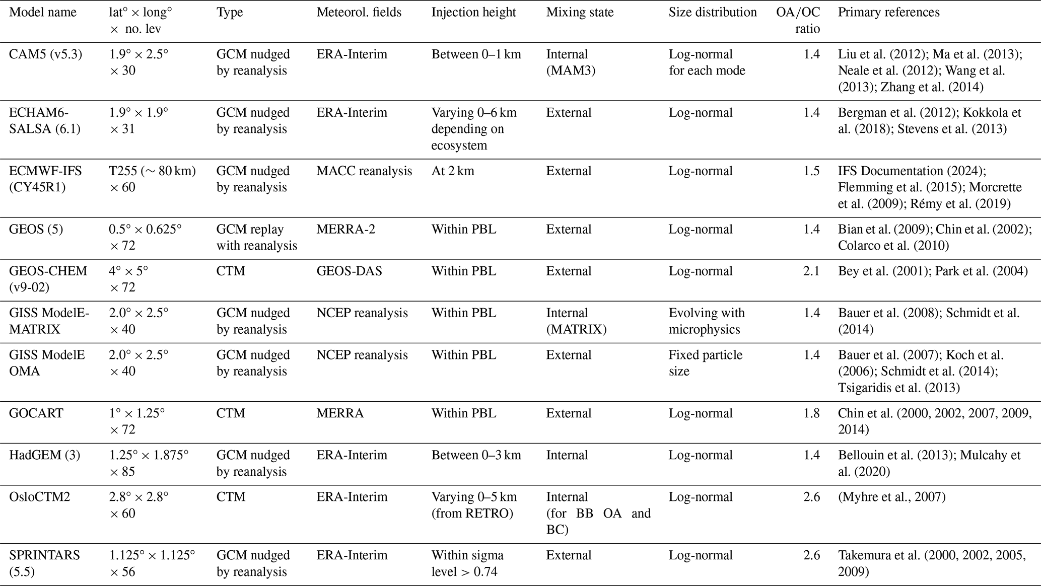
For the AeroCom-III BBESS experiment, 11 models submitted sufficient diagnostics to perform the analysis presented here. Information about model structure and model settings relevant to BB aerosol simulation for this experiment are listed in Table 1. Additional information on sources of aerosols other than BB smoke, and assumed particle microphysical properties for the 11 models, are included in Tables S1 and S2 in the Supplement. The models represent a diversity of spatial resolutions, parameterizations, and assumed particle sizes and properties. For example, the horizontal resolution ranges from about 0.5°×0.625° (GEOS) to 4°×5° (GEOS-CHEM), and vertical layers range from 30 (CAM5) to 85 (HadGEM). Meteorological fields were obtained from different reanalysis products. Although the modelers were asked to distribute BB emissions within the model boundary layer, some models chose to prescribe other BB emission injection altitudes (Table 1). For example, CAM5 injected smoke evenly within the lowest 1 km; ECMWF-IFS-CY45R1 distributed the amount within the lowest 2 km; OsloCTM2 incorporated a geographically varying injection height, with a maximum height of 5 km; and ECHAM6-SALSA injected the smoke between 0 and 5 km, depending on the ecosystem. Models with internal aerosol mixing assume homogeneous mixing and use some form of Mie scattering to calculate the optical properties of BB aerosol.
Table 1Participating models in this study with information relevant to biomass burning aerosols.
The year 2008 was selected as the “benchmark year” with prescribed daily biomass burning emissions from GFED3.1 for this study. Among the reasons for selecting this emission dataset and simulation time period were to examine the robustness of the analysis done for the single-model simulation presented in P2012 and P2017 and to evaluate the multi-model results with hundreds of satellite-observed cases compiled in previous studies (summarized in Sect. 2.3). Other aerosol emissions, including emissions from desert dust, fossil fuel combustion, and other anthropogenic and natural sources, were determined by the individual models.
In this study, we are using model output from two simulations, namely a control run (BB1) with all sources, including prescribed daily BB emissions from GFED3.1, anthropogenic emissions from a number of external emission inventories (Table S1) chosen by the modeling groups, and natural sources such as dust and sea salt calculated by the models and a run with the same sources but with no BB emissions (BB0). The difference between BB1 and BB0 allows the BB contribution to be isolated from other contributions to the aerosol load. In addition to these baseline simulations, the models performed three perturbation runs with the GFED3.1 daily emissions multiplied by factors of 0.5 (BB0p5), 2 (BB2), and 5 (BB5), respectively, to create an ensemble of four runs, where multiples of GFED3.1 represent a range of possible emission estimates for the same fires. The models were run for the full year and preceded by a 3-month spin-up.
2.2 The GFED BB emissions
GFED is one of the most widely used BB emission inventories in the global modeling community. It is also continuously updated to include the latest findings in BB emission development studies (Chen et al., 2023; Giglio et al., 2013; Randerson et al., 2012, 2017; van der Werf et al., 2017). At the time when the AeroCom BB experiment was proposed, GFED3.1 (Mu et al., 2011; Randerson et al., 2013; van der Werf et al., 2010) was the latest GFED version available. It was, therefore, used for the model runs performed for the current study. GFED3.1 provides daily biomass burning emissions of CO, SO2, NOx, NH3, VOC (volatile organic compound), BC (black carbon), and OC (organic carbon). The map of the 2008 annual GFED3.1 emission of OC, the most abundant primary aerosol species emitted from fire, is shown in Fig. 1a.
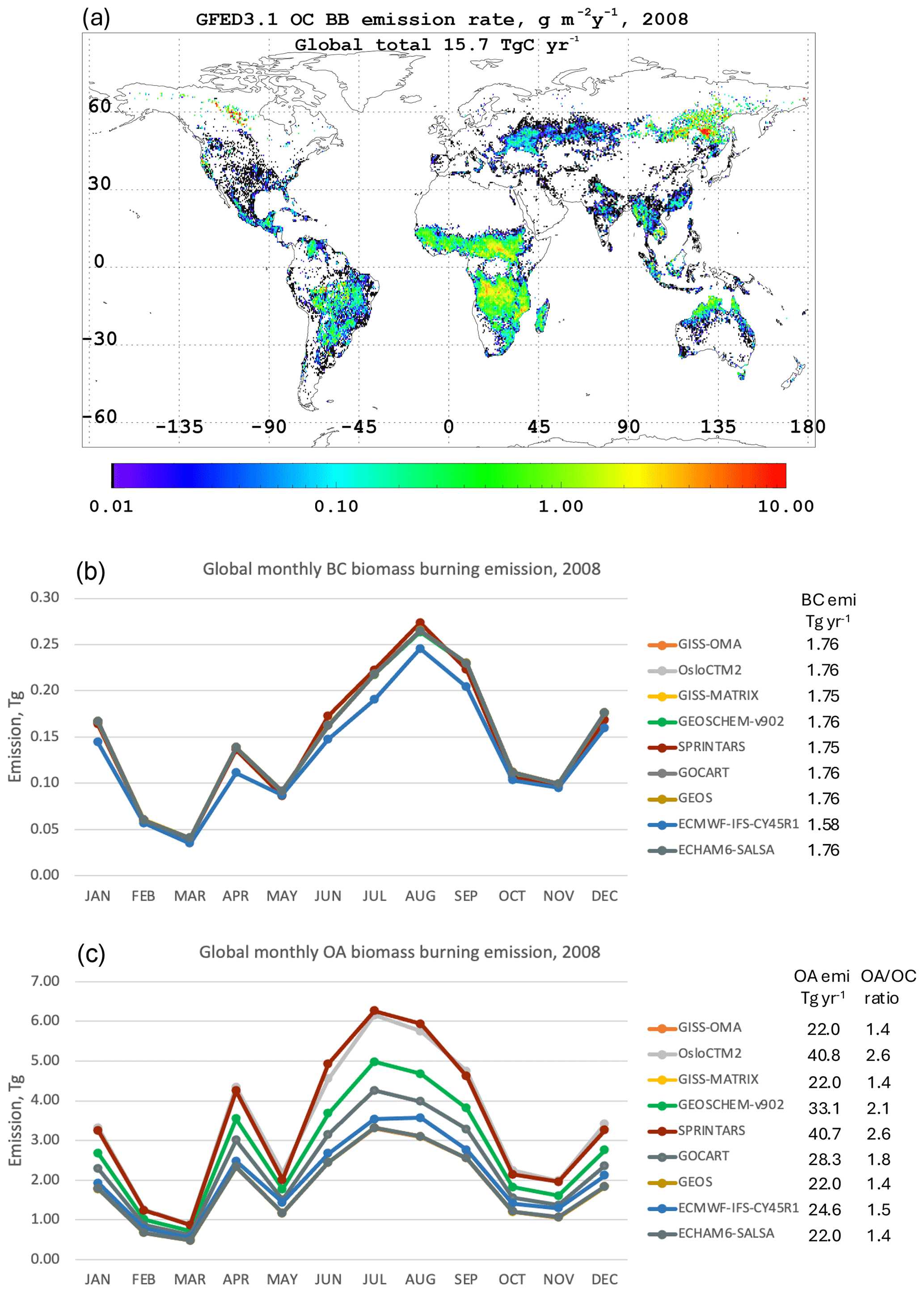
Figure 1Global biomass burning emissions of carbonaceous aerosols. (a) Annual emissions of OC in 2008 from GFED3.1. (b) Monthly BC emissions implemented in 9 out of 11 participating AeroCom models (BB emissions were not available from CAM5 and HadGEM3). (c) The same as panel (b) but for OA that is converted from OC with the ratio of the model's choice (listed in the legend to the figure). (Note: colored lines in panels b and c can overlap for models with identical emissions).
The later version, GFED4.1s, became available after the model runs were performed, using the newer GFED dataset in Sect. 5.
The global monthly BB emissions of BC and organic aerosol (OA) implemented in each model are shown in Fig. 1b and c, respectively. Unlike the nearly identical BC emissions from all models (Fig. 1b), the OC emissions provided by GFED3.1 had to be converted to organic aerosol mass (OA; also known as organic matter or OM) by multiplying OC by an ratio that is based on information from various observations. However, in reality, this ratio depends on the chemical age of OA, the particular OA species, and environmental conditions; it therefore can, in general, have a wide range of values, typically from a little over 1 to well above 2 (e.g., Aiken et al., 2008). As a result, although the same OC emissions are prescribed, the primary OA from BB emissions varies among the models by nearly a factor of 2, with OsloCTM2 and SPRINTARS having the highest values (2.6) and CAM5, GISS, GEOS, HadGEM3, and ECHAM6-SALSA having the lowest (1.4), as listed in Table 1 and illustrated in Fig. 1c. Figure 1 also shows that a primary emission peak occurs in July–August, which is when burning tends to favor northern mid-to-high latitudes and the southern subtropics; secondary peaks occur in December–January, which is when burning occurs preferentially in the northern hemispheric tropics, and in April, which is when burning takes place mainly in central America and southern Siberia (see Fig. 2 and Giglio et al., 2006a).
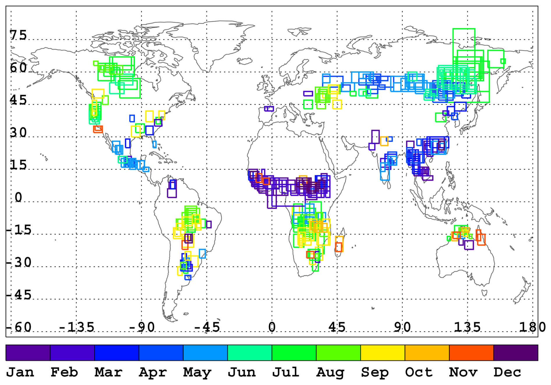
Figure 2Locations and months of the fire case boxes in this study.
2.3 The MODIS BB plume AOD dataset
We use the MODIS Collection 6 Level 2 AOD retrievals at 550 nm and 10 km resolution from the Terra and Aqua satellites as the key observational dataset to evaluate and constrain the models. The MODIS BB plume AOD dataset was introduced and refined in P2012 and P2017, respectively. Here, 447 fire/smoke cases in different biomass burning regions that fall within the benchmark year of 2008 are selected as the reference observational dataset from about 900 identified in P2017. The main criteria for selecting BB cases are detailed in P2012 and P2017; briefly, these include (1) plumes with at least one linear dimension of 100 km to be useful for global modeling studies with fairly coarse resolution of 1° or larger (Table 1), (2) a coordinated pattern of elevated AOD, (3) a visible smoke plume in the satellite imagery, and (4) a fire signal in the MODIS thermal anomaly product (MOD14). The locations and seasonality of the cases in the database are shown in Fig. 2. Note that fire activity in Alaska, Indonesia, and southern Australia was rather weak in 2008, so no cases were specified in these regions.
A comparison of the model instantaneous output matched to the snapshots of actual fires around the globe provides a unique perspective, complementing the usual model–satellite intercomparison that applies some spatial and temporal averaging. This study presents a test of how well and how consistently the models perform in simulating actual fire events. The observational dataset of fire/smoke events at the time they actually occur in different BB regions and seasons provides a way to assess the models, and this is distinct from typical model output analyses. The fact that this study reaches coherent results and comes to some conclusions that are similar to those of previous studies despite using different methods (e.g., Gliß et al., 2021) helps validate the effort. Other conclusions are obtained as well.
There is currently no algorithm of which we are aware that differentiates the BB portion of the AOD from the contributions of other aerosol types in the MODIS data (except possibly over dark water and based on the assumption that the coarse mode is essentially dust or sea salt, and fine mode is BB or pollution; e.g., Kaufman et al., 2005). Therefore, to estimate BB AOD from MODIS, we first estimate the background AOD value, i.e., AOD from non-biomass burning sources for each case box (defined below), by determining the most frequent mean pixel AOD within the case box over the 16 years (2000–2015) of available MODIS Terra data during the pre-burning-season month in that box and then subtracting this value from all the MODIS AOD values in the box during the BB event, as done in P2017. Before subtracting these “background” values, missing MODIS AOD retrievals within the plumes are filled with MERRAero reanalysis values (Buchard et al., 2015; da Silva et al., 2015), and scaled to retrieved MODIS AOD values in immediately surrounding locations for which MODIS and model values are available (details are presented in P2017).
Of course, this approach has limitations due to the interannual variability in burning and the variability in other aerosol sources. There is also the need to correct for possible negatives in the BB AOD values obtained in this way, as not all retrieved 10 km pixels are above the historically most frequent AOD background value. We set these to zero BB AOD to obtain a physically meaningful AOD value; this possibly introduces a positive bias into the averaging process, though only the lowest AOD values in the distribution are affected. A more detailed analysis of this BB AOD separation approach is presented in P2017; in summary, the “zeroing of negative BB AOD values” has the least effect in forested regions (such as those in group A; see below), and the largest number of negative BB AOD values replaced by zero occurs in AUST (Australia), followed by NHSA (northern hemispheric South America) and CEAS_W (central Asia west), which is consistent with the low MODIS AOD values in these regions.
2.4 Biomass burning regions
Based on the analysis in P2017 and the regional characteristics of fires, our analysis in the current study focuses on the same geographical regions. To better associate our analysis with other biomass-burning-focused studies (e.g., Giglio et al., 2006b; Mezuman et al., 2020; Pan et al., 2020; Rabin et al., 2015), we adopt the region names used by GFED (Giglio et al., 2006b) and assign our cases to these regions (Fig. 3). In addition, we further divide the BOAS region into eastern (BOAS_E) and western (BOAS_W) subregions and CEAS into eastern (CEAS_E) and western (CEAS_W) parts, mainly to account for observed differences in burning patterns within the broader GFED regions. In total, 13 regions/subregions are included in the current study. The regions are shown in Fig. 3, and the BB cases within each region are displayed as symbols, with different symbol styles assigned to distinctive groups based on the degree of concurrence between the satellite and model BB estimates, as discussed in the next section.
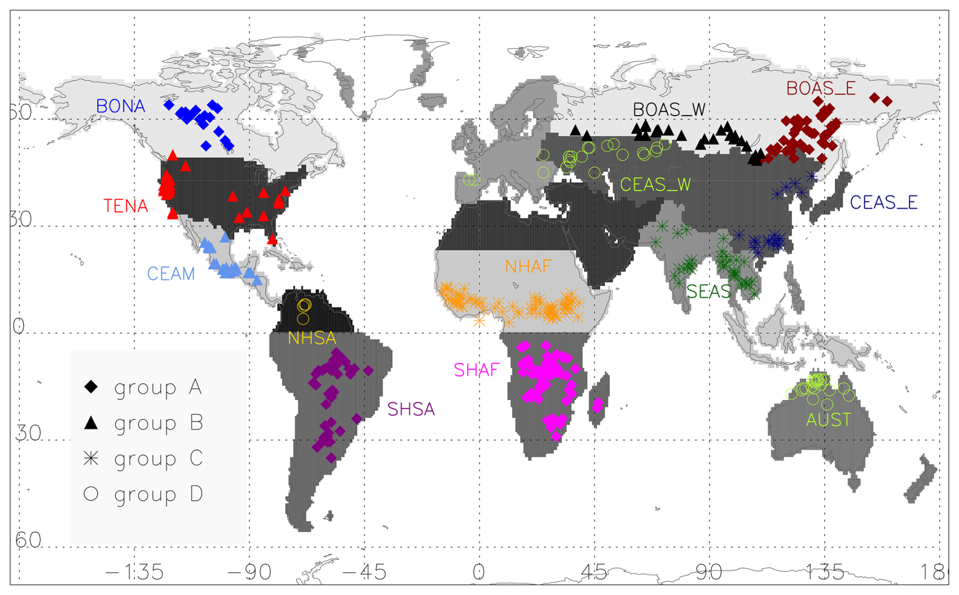
Figure 3The 13 regions with the BB cases in each region. BONA is for boreal North America, TENA is for temperate North America, CEAM is for central America, NHSA is for northern hemispheric South America, SHSA is for southern hemispheric South America, NHAF is for northern hemispheric Africa, SHAF is for southern hemispheric Africa, BOAS_W is for boreal Asia west, BOAS_E is for boreal Asia east, CEAS_W is for central Asia west, CEAS_E is for central Asia east, SEAS is for southeast Asia, and AUST is for Australia. Symbols for BB cases mark the group (A, B, C, or D) to which the BB region belongs. The groups of BB regions are explained in Sect. 3.2.
2.5 Comparing average values
We first clarify that all AOD values in this paper refer to the AOD at 550 nm. In order to compare BB emissions and BB AOD between models, we obtain model BB AOD by subtracting results of the no-BB-aerosol simulation (BB0) from the control run with all emissions (BB1). The method for obtaining MODIS BB AOD is detailed in P2017 and is briefly summarized in Sect. 2.3 above. We then use the instantaneous model output closest in time to the satellite observation to calculate case average values. As each rectangular case box is defined by a set of latitude–longitude coordinates, the model output was sampled to include all the grid boxes for which the centers fall within the case box. Average values from MODIS and the models were then compared over the area of the box. In comparing models and satellite observations with a different resolution over a set of boxes varying in size, we have chosen to average the variables of interest over each case box. More considerations on the use of case box as the unit of comparison are provided in Sect. S1.
When comparing values in further analysis, we calculate average values in the following ways:
-
The case box average AOD (also for BB AOD, load, loss, and extinction efficiency) is the arithmetic mean of all AOD values within a case box. For BB AOD, we first subtracted the background AOD (a fixed, pre-determined, and case-specific value for MODIS and the no-BB run for models) from all AOD pixels in the case box to obtain BB AOD. Then we set any negative BB AOD values to 0 and average BB AOD over the case box.
-
The regional average is the simple arithmetic mean of all average case values for cases assigned to the region.
-
The all-case average AOD (or BB AOD) is the simple arithmetic mean of all average case AOD (or BB AOD) for all 447 cases in the study.
-
The global monthly values include all grid boxes weighed by area and averaged over a month (used for model-to-model comparisons only).
When working with variables that represent ratios of values (such as model-to-satellite AOD ratios, loss rate, or mass extinction efficiency), the robust mean is often used to exclude any values falling beyond 4 standard deviations of the mean to discard outliers. This approach ensures that, in regions with very low AOD values, the ratios of a few very small numbers do not skew the regional averages unreasonably. This treatment rejects 0 %–10 % of the case values from contributing to the regional averages.
3.1 Comparisons between MODIS and model BB AOD cases over biomass burning regions
Figure 4 shows the spatial distribution of simulated BB AOD relative to the estimated MODIS BB AOD described in Sect. 2, covering all the individual cases for each model. The models are ordered from the highest to lowest overall BB AOD (when all cases are averaged, which is quantified in the “Multi-region mean” row in Table 2). Many common features among the models relative to MODIS appear in Fig. 4. For example, the models report generally lower BB AOD than the MODIS estimates, except in some cases in central and southern Africa. However, most do fall within 50 % (ratio between 0.67–1.5) of the MODIS-derived values over the boreal region of North America (BONA), southern and parts of central Africa (SHAF – southern hemispheric Africa; NHAF – northern hemispheric Africa), northern Venezuela/Columbia (NHSA), and northern Australia (AUST). The model BB AOD simulations tend to be much lower over the USA (temperate North America – TENA), Mexico (CEAM – central America), western boreal region of Asia (CEAS_W), central and southeast Asia, China (CEAS_E), and India (southeast Asia – SEAS), generally by factors of 5 to >10.
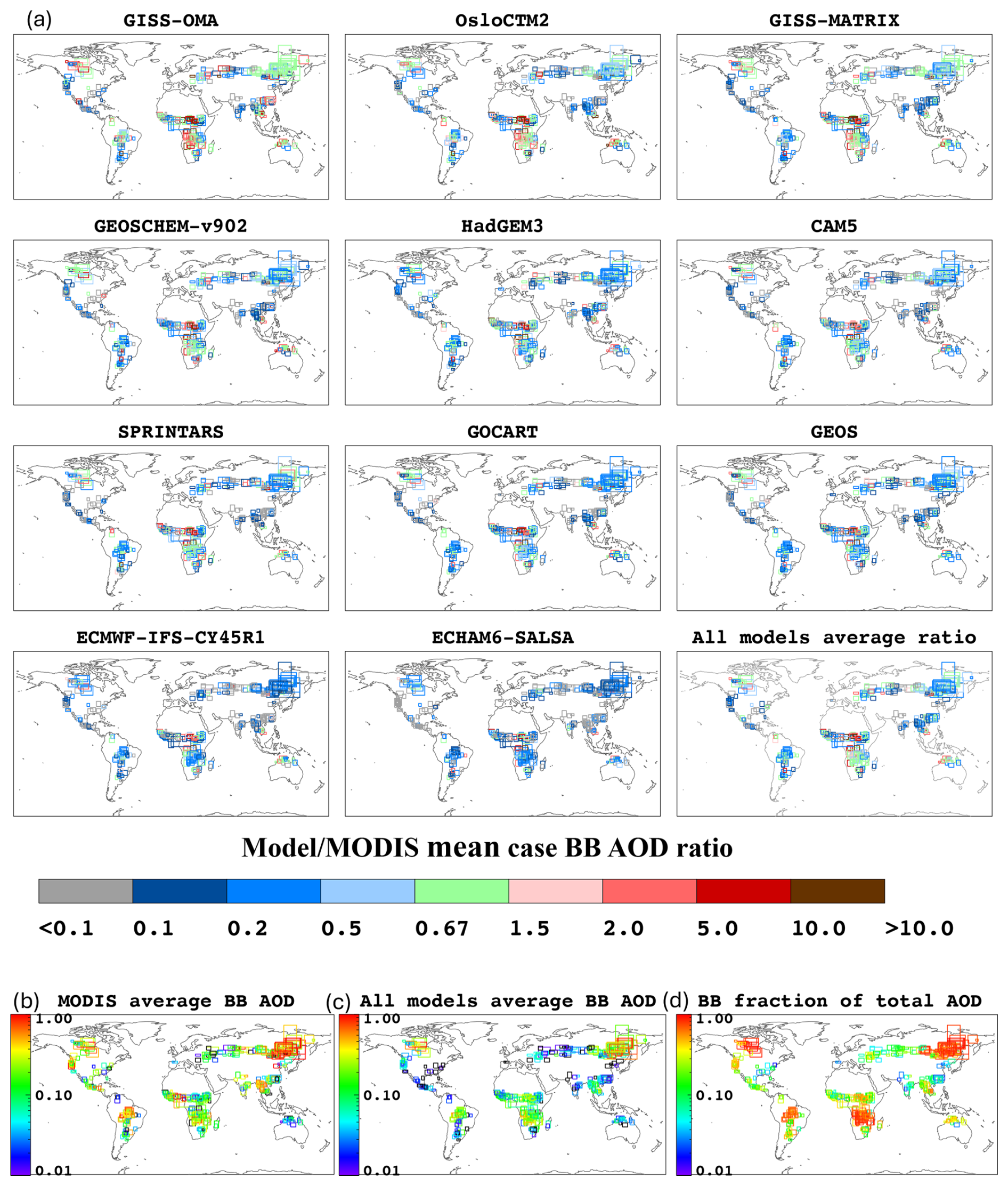
Figure 4(a) Ratio of model-simulated BB AOD (from model experiment BB1–BB0) to the BB AOD derived from MODIS for all individual fire cases for each individual model, and (bottom-right panel) the multi-model average of these ratios for all study cases. (b) BB AOD derived from MODIS for reference. (c) BB AOD averaged across all models. (d) BB AOD fraction of total AOD averaged across all models for all study cases.
Table 2Ratios (r) of model-calculated BB AOD to MODIS-derived BB AOD for cases within each of the 13 regions. Colors illustrate the bias of individual models relative to MODIS. The means, standard deviation, and diversity are also tabulated. Regions are further grouped into A, B, C, and D, based on the degree of agreement between multiple models and MODIS to help discussion.
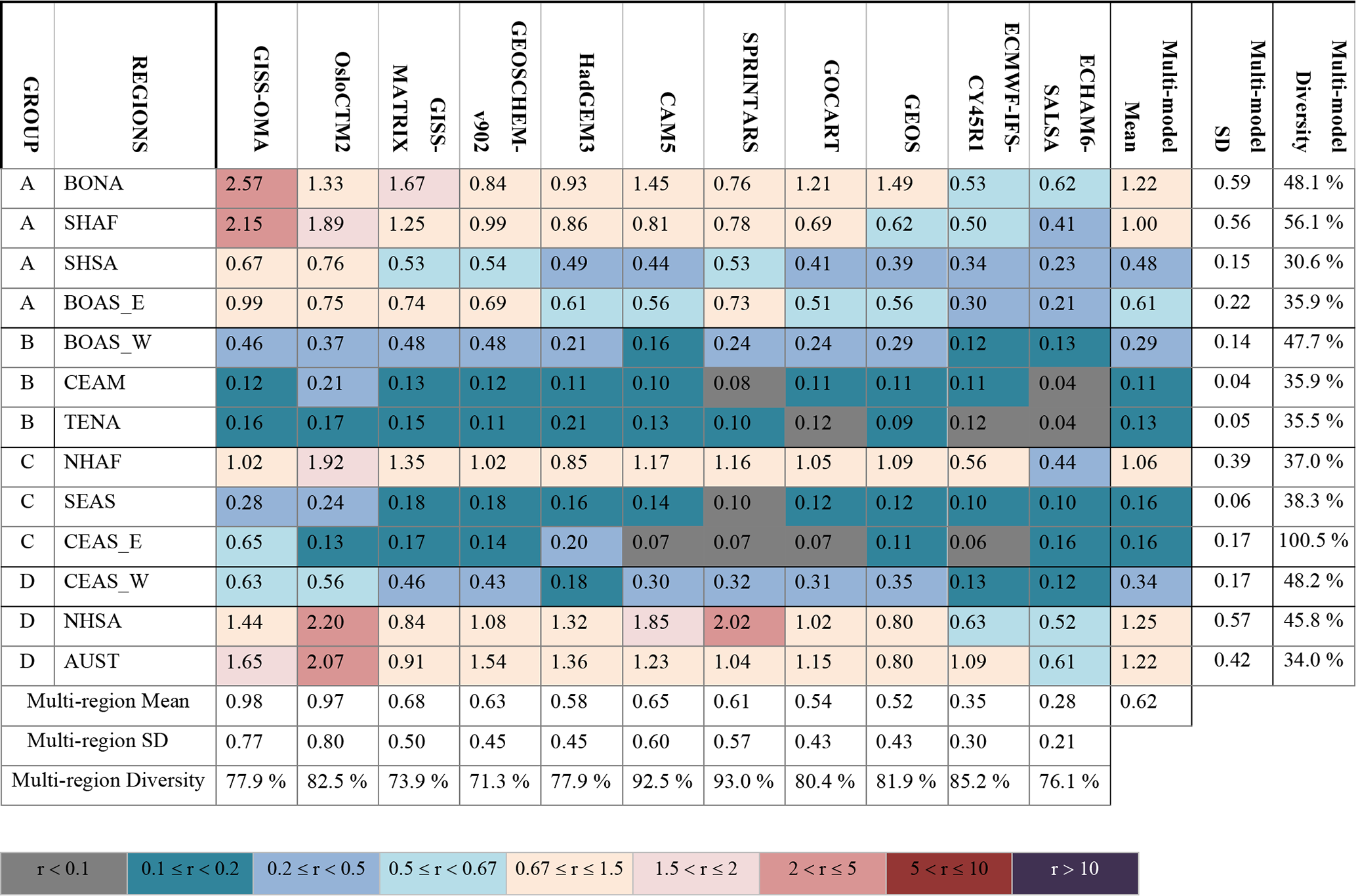
These model-to-MODIS BB AOD ratios are enumerated in Table 2 for all models and all regions. To make discerning regional patterns easier, the table cells are colored according to the color scheme in Fig. 4. These color clusters in Table 2 emphasize the spatial patterns described above. The third-to-last column of the table contains the multi-model BB AOD mean for the region (mean of model regional means in the corresponding row of the table), showing that models generally tend to output higher or lower AOD in the region, and the last two columns show the standard deviation and the diversity (defined as ratio of standard deviation to the mean; expressed in percent) of the values from all the model means in the region, where lower diversity corresponds to greater consistency in model performance in the region. Here and subsequently, we calculate diversity as the ratio of the standard deviation of the array and its mean (expressed in percent). The bottom rows of Table 2 contain the standard deviation and inter-regional diversity for each model, showing that some models, e.g., GISS-OMA and OsloCTM2, have an overall mean AOD ratio close to unity but with a higher variation between regions (higher standard deviation, SD), whereas others, such as ECMWF-IFS-CY45R1 and ECHAM6-SALSA, are more consistently biased low across all region, though their relative diversity may be comparable.
The regions are further collected into groups A, B, C, and D, as discussed in the Sect. 3.2. A deeper dive into the absolute values of BB variables for each model in each region is available in Fig. S3.
3.2 Separating BB regions into different groups
To compare multiple variables for 11 models over 13 regions comprehensively, we developed a multi-factor region–comparison approach. For example, in P2017, we considered the magnitudes of total MODIS and model AOD, biomass burning fraction of total AOD, and model/satellite BB AOD ratio to assess how effectively our method of estimating the source–strength by comparing modeled and measured AOD can be used in different BB regions.
We begin here by stratifying the regions into groups according to several observation-based criteria that reflect the level of confidence in our ability to identify the MODIS and the model BB AOD components. The criteria for grouping regions are as follows:
-
Total AOD from MODIS. MODIS AOD retrieval uncertainties are much lower when the AOD is above about 0.1 (Levy et al., 2013). So, under the conditions when MODIS AOD is sufficiently high if the total AOD discrepancy between the models and MODIS is large, it is likely an issue with the models, such as emission strength or model processes and assumptions. This provides important regional information in the context of the current study. If the total AOD from MODIS is low, then the relative uncertainty in the estimated MODIS BB AOD is expected to be high.
-
Biomass burning AOD fraction from MODIS when total AOD is high. If the BB AOD fraction (fBB) is also high (i.e., the estimated background non-BB AOD fraction is low), we have greater confidence in the MODIS BB AOD obtained by subtracting the estimated background AOD from the total AOD. Otherwise, the estimated MODIS BB AOD is more uncertain.
-
Total AOD and BB AOD from models. If the total AOD and BB AOD fractions from the models are relatively high, we are more certain that our constraints can be applied to assess the biomass burning emission source strength, as intended. Otherwise, more issues related to the model simulation of BB and other (background) aerosol types (pollution, dust, etc.) complicate the interpretation of the results.
Figure 5 is a flowchart showing the process we applied to assign regions to particular groups, using the three criteria listed above. Overall, the 13 biomass burning regions in Fig. 3 are associated with groups A, B, C, or D, based upon the process described in Fig. 5.
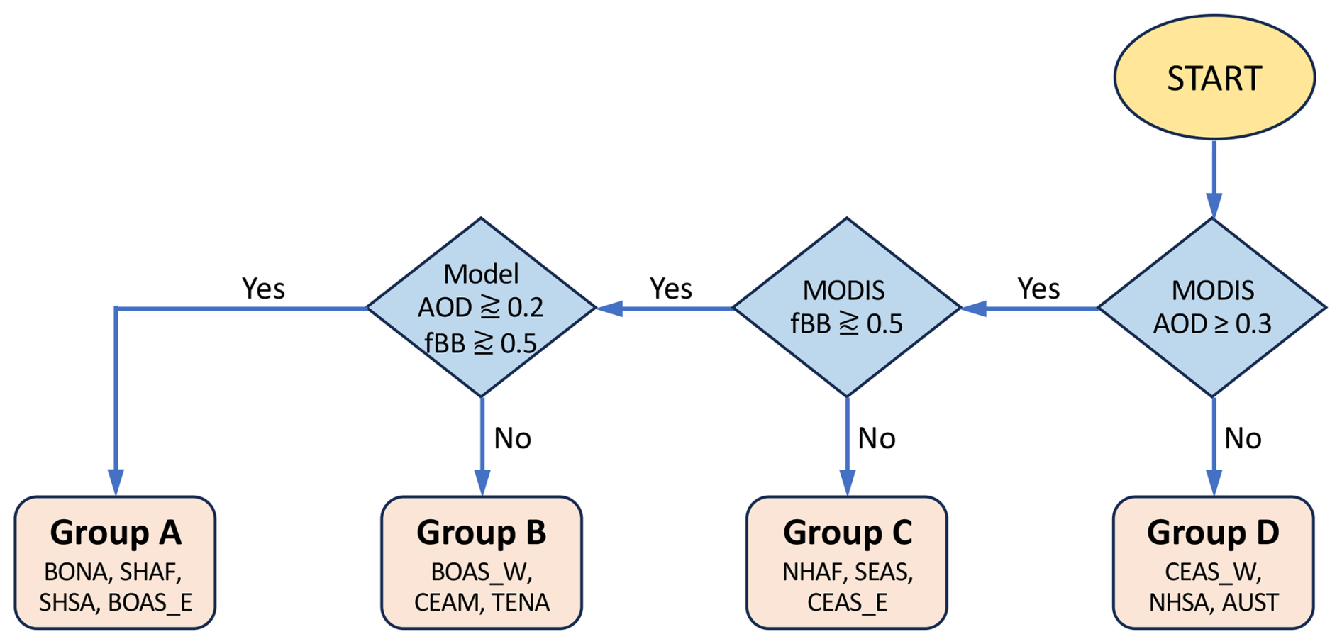
Figure 5Flow chart of the procedure used to separate the 13 biomass burning regions into four groups having distinct characteristics in biomass burning intensity, fraction of smoke AOD within the total AOD (fBB), and differences between the quantities from MODIS and the multi-model mean. Regions in each group and their characteristics are shown in Figs. 3 and 6.
A quantitative representation of regional all-model means for these criteria is provided in Table 3. To make discerning regional patterns of factor magnitudes in Table 3 easier, we used bold font to show the values of the factors in the regions where they exceed the empirically chosen threshold. As such, the regular and bold fonts in the table represent qualitative criteria favorable for applying the satellite AOD to constrain emission source strength in the models, with values above the threshold being more favorable and those below being less favorable.
Table 3Multi-factor comparison of BB regions.
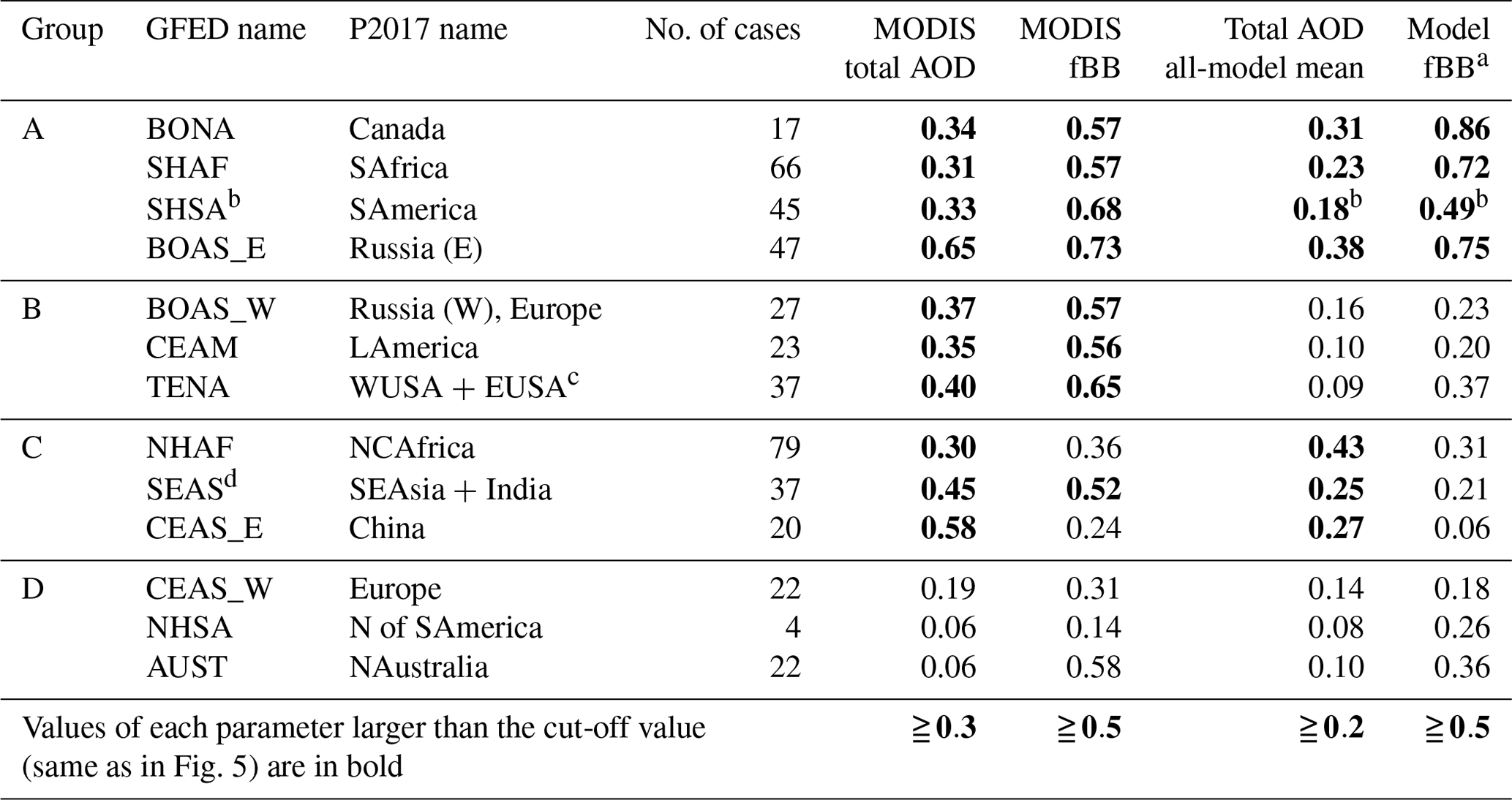
a fBB is a fraction of total AOD attributed to biomass burning aerosol. b Total model AOD and model fBB are rounded up to 0.2 and 0.5, respectively, putting SHSA in group A. c WUSA is west USA, and EUSA is east USA. d Even though MODIS fBB in SEAS is higher than the cutoff threshold for group C, the complex aerosol mixture in this region makes our confidence in MODIS background AOD values (and thus in MODIS fBB of 0.52) rather low, and the combination of fairly high model AOD and low BB AOD fraction in the models puts this region in group C.
3.3 Broad view of MODIS and model comparisons in biomass burning regions and groups
We present a broad view of MODIS and model comparisons by region in Fig. 6. The general model behavior is represented by the multi-model mean values of AOD and BB AOD. We show in Fig. 6 (top panel) the total AOD (stacked bars), as well as BB and background AOD from MODIS (dark red and blue bars, respectively), and the corresponding multi-model mean values (light red and blue bars) averaged for cases that fall within each region. The 13 regions are divided into the four regional groups, designated earlier as A, B, C, and D, based on physical criteria (Sect. 3.2). Also shown are the BB AOD fractions for MODIS and for the model means in dark and light red lines, respectively. The ratios of model mean total AOD, background AOD, and BB AOD to the corresponding MODIS quantities are shown in the bottom panel of Fig. 6 with solid, dashed, and dotted-dashed lines, respectively.
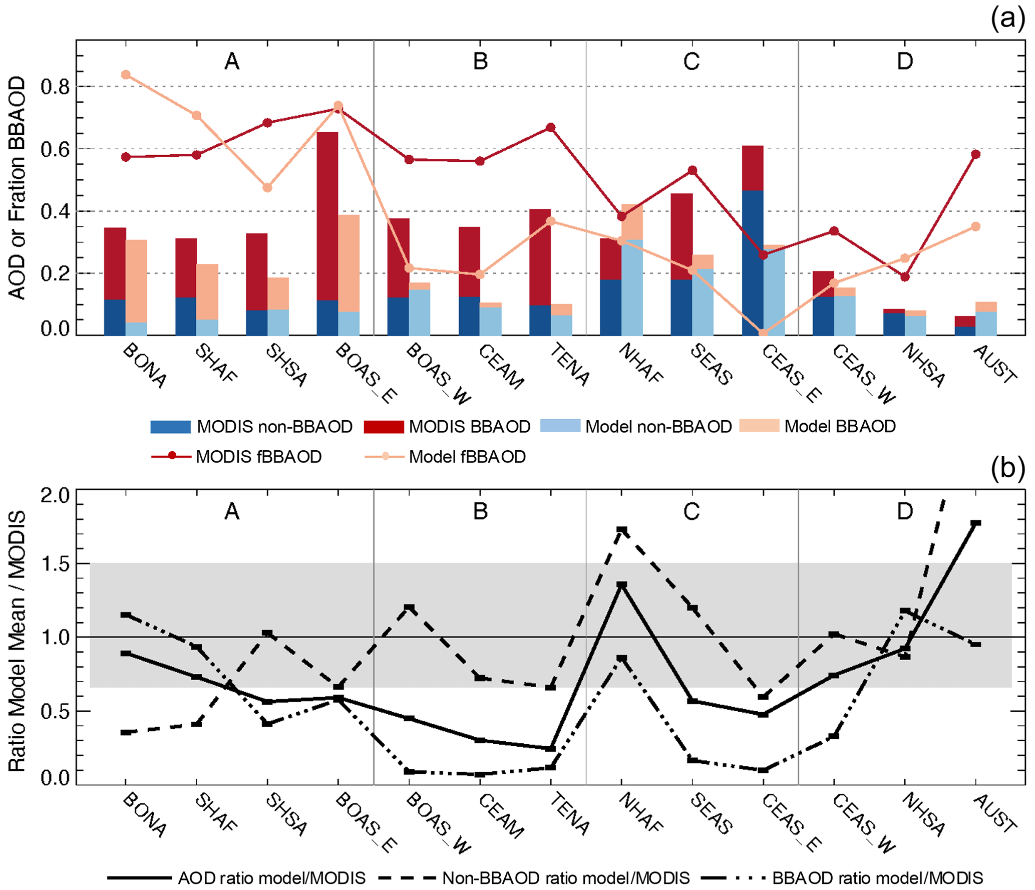
Figure 6(a) Total AOD from MODIS (stacked dark red and shaded blue bars) and from the multi-model mean (light stacked red and shaded blue bars), the corresponding BB AOD (red colors) and non-BB background AOD (blue colors), and their BB AOD fractions (lines) averaged for cases in each of the 13 regions grouped by A, B, C, and D (see Fig. 5 and the text). (b) Ratios of the model mean to MODIS for total AOD (solid line), BB AOD (dotted-dashed line), and non-BB background AOD (dashed line). The shading in light gray indicates the range of the model-to-MODIS ratio (R) within 50 % ().
Four regions (BONA; SHAF; SHSA – southern hemispheric South America; and BOAS_E) fall into group A, where AOD and BB AOD fractions from both MODIS and model means are generally high (AOD≥0.3 for MODIS and 0.2 for the model mean; BB AOD fraction 0.5 for both MODIS and the model mean). Tree cover dominates in these regions, with few other aerosol sources and typically well-defined fire plumes or major burning events (see also Table 4 in P2012 and Fig. 1a in P2017).
Unlike group A, the model mean AOD and BB AOD are both dramatically lower than MODIS in group B, by factors of 5–10 for AOD (solid line; bottom panel in Fig. 6) and around 20 for BB AOD (dotted-dashed line; bottom panel in Fig. 6). However, for the group B regions, the non-BB background AOD between MODIS and the model mean agrees to within 50 %, with the ratio of model/MODIS for non-BB AOD=0.67–1.2 (dashed line; bottom panel in Fig. 6). Given the high AOD and >0.5 BB AOD fractions based on MODIS, and the agreement between MODIS and the model on background AOD, we are more confident in suggesting that the GFED3.1 BB emission is systematically low or has missed significant sources in the group B regions. A high bias in MODIS total AOD and low bias in our MODIS background subtraction possibly also contribute, but this is less likely.
Although the total AOD from MODIS in group C is of similar magnitude to that in groups A and B, the fraction of BB AOD is much lower. Regions in group C contain BB cases with a variety of trees and shrub, grass, or cropland vegetation types but are heavily influenced by either dust (in NHAF) or high pollution (in SEAS and CEAS_E), making the MODIS background subtraction as well as the model-simulated BB contribution to the total AOD more uncertain for this group. Meanwhile, the non-BB background AOD is higher for the MODIS (0.18–0.46) and model mean (0.21–0.31) than for any other group. Such high non-BB AOD fractions reduce the confidence in our BB source–strength estimates in these regions.
In group D, MODIS total AOD is the lowest among all groups at 0.06–0.20, and the BB signal is very weak, resulting in BB AOD being estimated at 0.015–0.08. As such, small errors in any aspect of the MODIS retrievals can produce large relative uncertainties. Among the regions in group D, the AUST fire cases are mostly in areas with deciduous shrub cover, and CEAS_W is dominated by cultivated and managed lands. There are only four cases for NHSA, so statistics for this region are not robust. Although the model mean AOD and BB AOD generally agree with the corresponding MODIS values within a factor of 2, the confidence in our source–strength estimates in the group D regions is limited because of the low signal in the observations.
From the above analysis, we reach a few conclusions about biomass burning emissions of GFED3.1 used by the models. The biomass burning emissions are most likely to be realistic in group A regions, but they should be increased by a factor of 2–10 in the group B regions for the models to come into line with the satellite BB AOD, based on the agreement between model and satellite data for the background non-BB AOD. Model results from the BB5 run (BB emissions increased by a factor of 5) yield a model-to-MODIS BB AOD ratio of around 0.7 for TENA, 0.6 for CEAM, and 2.5 for BOAS_W, suggesting that multiplying aerosol emissions by 2 in BOAS_W and by almost 10 for TENA and CEAM would make the model and MODIS BB AOD comparable. Because of the high non-BB (background) AOD fractions in group C, and the low total AOD and BB AOD in group D, we do not have sufficient confidence to draw conclusions about biomass burning emission strength over regions within these groups.
4.1 Multi-model means of BB OA quantities in each region
We show in Fig. 7 that the multi-model mean quantities of BB OA mass load (green bars), loss rate (purple bars), and the mass extinction efficiency (MEE; orange line) convert the model BB OA mass to BB OA AOD in all cases of each region. As expected, more and/or larger fires in the regions of group A correlate with higher BB aerosol loads. The residence time, related to OA removal from the atmosphere in each region, can be estimated by dividing the load by the loss rate; from the relative heights of the green and purple bars for each region in Fig. 7, we estimate the different residence times of OA among regions. For example, in group A, OA residence time in boreal regions BONA and BOAS_E (higher purple bars than green) is shorter than that in SHAF and SHSA (higher green bars than purple), reflecting the differences in the mass balance of smoke aerosol emission, deposition, and transport fluxes in each region. On the other hand, the multi-model mean OA MEEs, calculated as the ratio of BB AOD to BB load here, are similar across the regions in all groups (3000–4000 m2 kg−1), despite large differences in BB OA mass or load in these regions. However, despite this region-by-region similarity of mean values (generally between 3000 and 400 m2 kg−1), MEE diversity among individual models is remarkable, as seen from the large MEE standard deviations in each region. Details of individual model values by region are provided in Fig. S2. As much as Fig. 7 demonstrates the general aerosol and fire features in different BB regions and is based on the averages of individual and specific BB cases, the characteristics of the models that would describe their performance are explored in the Sect. 4.2, based on the global averages of variables.
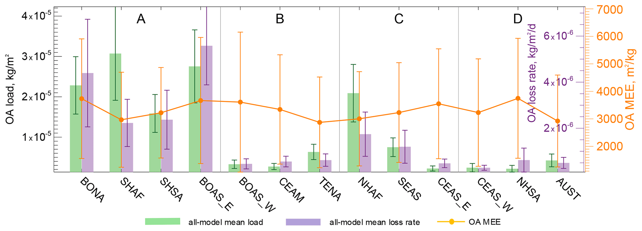
Figure 7Multi-model mean BB OA load (kg m−2; green bars; left y axis), multi-model mean BB OA loss rate (; purple bars; purple right y axis), and multi-model mean mass extinction efficiency of BB OA (m2 kg−1; orange points and whiskers; orange right y axis) averaged for cases in each of the 13 regions grouped by A, B, C, and D (see Fig. 5 and text). Whiskers show the standard deviations of the multi-model means, respectively.
4.2 Diversity in atmospheric processes and BB optical properties among models
Fundamentally, the column AOD reported by the models is derived from the aerosol mass loading in the atmosphere and the efficiency with which radiation is scattered and absorbed by the mass of a given aerosol species present, i.e., the MEE, under ambient atmospheric conditions. Globally, the total aerosol mass load within the models is the result of the total source (including primary aerosol emissions and secondary aerosol production) and removal processes (including dry and wet deposition and chemical loss). These factors control the aerosol amount and lifetime in the atmosphere. On the other hand, the MEE depends upon aerosol composition, size distribution, shape, particle density, refractive indices, aerosol mixing state, and hygroscopicity, which usually depends upon the ambient relative humidity.
Although the transport processes and regionally varying secondary organic aerosol (SOA) production rates (Carter et al., 2020) that affect aerosol spatial distribution might explain some of the model differences regionally, comparisons among the global values of the key quantities determining the BB AOD can shed light on the model diversity that underlies regional differences in a manner that is relatively independent of the transport. Here, we compare the individual model global values of five key biomass burning BC and OA quantities for 2008 in Fig. 8, namely emissions, lifetime, atmospheric mass loading, MEE, and BB AOD, which is expressed as the percentage departure of individual models from the multi-model mean, with the numerical value of the overall spread given below each parameter label. Among these quantities, the lifetime is calculated as the aerosol mass load (kg m−2) divided by the loss rate (), and the MEE (m2 kg−1) is obtained by the ratio of AOD to mass load (kg m−2). (Note that in taking the global mean of all the BB variables, we subtracted the BB0 from the BB1 model runs and then calculated global means, which effectively compares model characteristics in general and not just those assessed for the specific regions and cases that are considered elsewhere in this study.)
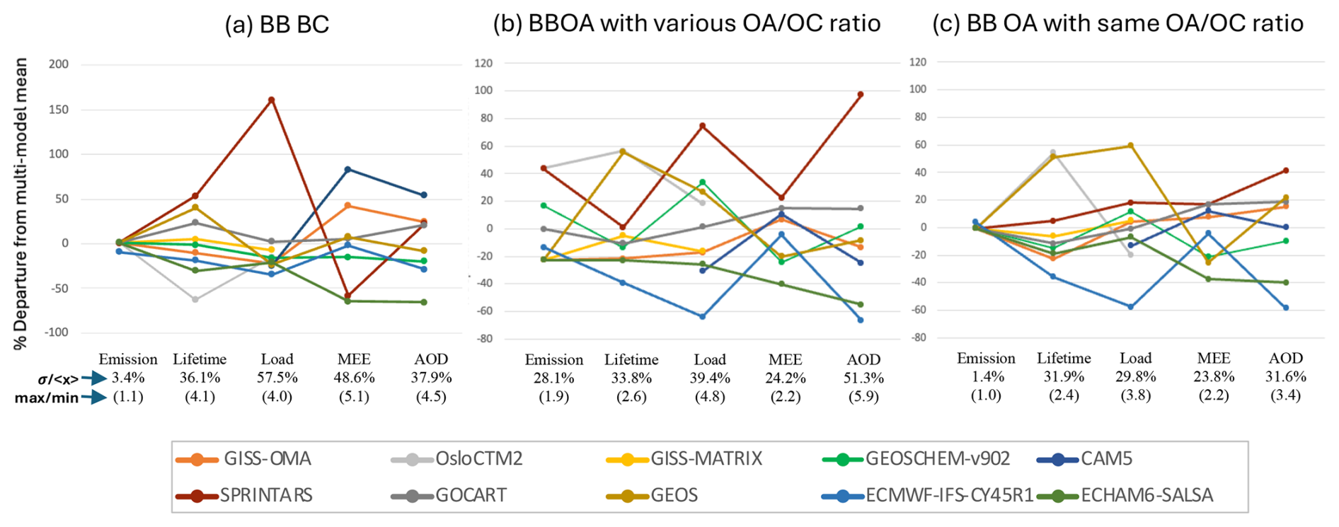
Figure 8Differences among model-simulated key parameters determining the (a) BC AOD and (b) OA AOD from biomass burning sources, expressed as the percentage departure of each model from the multi-model mean values. The quantities are derived from global mean values for 2008. The model diversity of each parameter, defined as the percent of the standard deviation/multi-model mean for each parameter is listed under the corresponding parameter. The spread of values, represented by the ratio of the largest of the model values for the corresponding parameter to the smallest, is given in parentheses under the corresponding diversity. (c) Same as panel (b) but with OAOC factors normalized across all models. (Note that emissions and lifetime are not available from CAM5, and HadGEM3 is not included here for the lack of all budget terms).
As shown in Fig. 1b, the BB BC emission rates implemented in the models are identical, as prescribed from GFED3.1, except ECMWF-IFS-CY45R1, which is 10 % lower than all other models, leading to a 3.4 % model diversity of the BB BC emission (Fig. 8a). In comparison, the diversity of the end-product of BB BC AOD is 38 %, which is more than 10 times higher than that of the emissions. Considering that the AOD is the product of mass load and MEE, it is remarkable that the diversity of BB BC AOD is lower than the diversities associated with the associated mass (58 %) and MEE (49 %). This can be explained by some compensating factors that can be seen in Fig. 8a. For example, SPRINTARS (Spectral Radiation-Transport Model for Aerosol Species) and GOCART have the same BC BB emission and the same BC BB AOD, but the BC load from SPRINTARS is 2.5 times larger, and the BC MEE is 2.5 times smaller than the corresponding values for GOCART. Also, notably, CAM5 has the highest MEE, making its simulated BC BB AOD the highest among the models, despite the moderately low BC BB mass loading. The results in Fig. 8a illustrate that the inter-model difference in BB AOD cannot be explained by the difference in the emission, but is driven by the differences in (a) BC load, governed by the removal processes (thus lifetime), and (b) MEE, determined by the particle physical and optical properties (including size, density, refractive indices, mixing state, and hygroscopic growth). Currently, neither of these is well constrained; this is primarily due to a lack of adequate observations.
The propagation of the inter-model differences from emission to AOD can be further revealed in the BB OA cases (Fig. 8b and c). As discussed in Fig. 1c, although all models use the same BB emissions for OC from GFED3.1, the different OAOC ratios chosen by individual models result in a difference of nearly a factor of 2 in OA emissions, producing an inter-model diversity of 28 % for emissions (Fig. 8b). Higher BB emissions generally lead to higher BB AOD globally, but this is only part of the story, as the diversity of BB OA AOD among the models (51 %) is much greater than that of their corresponding BB emissions overall. Some of the difference can be traced to the disparity of the BB OA emission rates that begins with OA emissions from SPRINTARS and OsloCTM2 being 80 % higher than that from ECMWF-IFS-CY45R1 and ECHAM6-SALSA because of the different OAOC ratios assumed (see Fig. 1b). On the other hand, some model behaviors are more difficult to explain. For example, globally, SPRINTARS and OsloCTM2 have the same OA emission rates, but the OA load from SPRINTARS is 60 % higher, despite having a 50 % shorter lifetime than that from OsloCTM2. Among all models, SPRINTARS produces the highest BB OA AOD that is 100 % higher than the multi-model mean, whereas ECMWF-IFS-CY45R1 and ECHAM6-SALSA are the lowest, at about 60 % lower than the multi-model mean.
To address the inter-model difference in the simulated BB OA AOD that is caused by the disparity of the OAOC ratios, we normalize the BB emission, load, and AOD for OA to a fixed common ratio and then re-calculate each term displayed in Fig. 8b. The results are compared in Fig. 8c. In this case, the diversity of emission becomes 1.4 % (the emission from ECMWF-IFS-CY45R1 is 4 % higher than all other models), and the diversity for BB OA AOD is reduced to 31.6 %, suggesting that using different OAOC ratios by the participating models in this study contributes to nearly 20 % of model diversity of BB OA AOD on global annual basis. Meanwhile, the diversity of the intensive properties, MEE, and lifetime remain the same as in Fig. 8b, as expected.
Another factor that adds diversity to the models' treatment of OA is the simulation of secondary organic aerosol (SOA). Previous studies (e.g., Carter et al., 2020, and references therein) suggest that SOA amount varies regionally and is very challenging to estimate both due to large possible variation in the POA and the lack of consistent and conclusive observations to constrain SOA sources. Among the models in this study, all emissions shown in Fig. 8 are for primary OA (POA), but BB OA AOD includes both primary and secondary organic aerosol (SOA) in the OsloCTM2, GEOS-Chem, and CAM5 models. In the attempt to work with total OA output provided by the models, whether the model includes SOA simulation or not, these three models also include SOA in their load and loss estimates, with BB SOA contributing around 5 % to loads and AOD of BB OA in CAM5 and OsloCTM2 and 15 % in GEOS-Chem, with these fractions being much smaller than the SOA fraction of the total (BB and non-BB) OA; furthermore, these values vary greatly, both seasonally and regionally, in all the models. Note that some models such as GOCART and GEOS have SOA produced from non-biomass-burning sources that are included in the total OA but not in BB OA.
In summary, although consistency among the models does not necessarily indicate an accurate representation of smoke plume properties and behavior, the model diversity does at least provide a lower bound on uncertainty. Individual and significant outliers point to areas where specific questions about model assumptions might be asked, and more generally, observations are clearly needed to better constrain loss mechanisms and MEE.
The multi-model diversity illustrated in Sect. 4 above highlights uncertainties in the key quantities in the model simulations of BB AOD, starting from emissions and propagating through atmospheric processes and the models' implementation of the aerosol physical and optical properties. These model uncertainties, compounded with uncertainty in the separation of MODIS BB and background AOD, limit the confidence with which any method combining satellite-retrieved AOD with model simulations can constrain source strength or other model attributes. However, having identified these limitations, we can at least apply the method in places offering the best conditions for assessing smoke source strength with this approach, i.e., the group A and possibly group B regions, with an appropriate consideration of the uncertainties involved in these areas. On the other hand, the analysis presented here underlines the limitations of this method, especially in regions with high non-BB aerosol fractions, such as several regions in groups C and D. This calls for the application of satellite measurements with more reliable BB AOD separation methods, such as having a multi-angle (e.g., Junghenn Noyes et al., 2022; Kahn et al., 2010) and possibly polarization, as well as multi-spectral sensitivity, (e.g., Dubovik et al., 2019) in global remote-sensing measurements.
Background AOD subtraction for BB AOD measurement estimation is likely to improve once tighter constraints on satellite-retrieved particle properties (e.g., Junghenn Noyes et al., 2022) become more widely available. Also, current global models may best be used to compare coarser-resolution variables, e.g., averaged over larger areas and over weeks or months, rather than comparing individual events. Our study indicates that focusing on snapshots of single events might require obtaining a larger sampling of cases in some regions and/or having models offering finer spatial resolution. Also, there might be other novel ways to run models that would better isolate specific sources and thus improve inter-model and model–measurement comparisons. As applied here, the approach works best for large and well-defined smoke plumes in low-background environments.
With all models significantly underestimating both total and BB AOD but matching the MODIS background AOD values within 50 % in regions of group B (TENA, CEAM, and BOAS_W), we infer that the inputs of aerosol source–strength to the models from the aerosol emission inventory are most likely too low in these regions. Regions of group B contain predominantly cultivated lands and mixed vegetation types. Both small fires and other factors likely contribute to the emission deficit in these regions that are probably severely underestimated in the GFED3.1 emission models used in this study. Although GFED has evolved since the model runs were performed using the newer version, GFED4.1s, that includes aerosol emissions from small fires (van der Werf et al., 2017), the BB emission of carbonaceous aerosol from GFED4.1s has increased only modestly (10 %–40 %) in the group B regions (Pan et al., 2020), which is certainly far from the factor of >10 increase needed for models to match the MODIS BB AOD. In that regard, some more aggressive BB emission estimates, such as the Quick Fire Emission Dataset, QFED2.4 (Darmenov and da Silva, 2015), which is based on the MODIS fire radiative power (FRP) and optimized with the MODIS observed AOD in the BB regions, could produce a closer agreement between model and observations in some of the model-underestimated places, such as regions in group B; the QFED2.4 emissions are 4–16 times higher than GFED3.1 in these regions (Pan et al., 2020). Other aspects of the model treatment of aerosol microphysical and optical properties, such as size distributions, mixing states, hygroscopic properties, and MEE, will also affect the BB AOD calculations.
Another emission-related issue is the choice of OAOC ratios by individual models that vary by a factor of 2 from 1.4–2.6 (Table 1 and Fig. 1c). This range is justified, as available observations show similar ranges of values, such as 1.4–2.1 (Turpin and Lim, 2001), 1.8 (Hand et al., 2012), 1.3–2.1 (Philip et al., 2014), and 2.2–2.5 (Hodzic et al., 2020). In reality, the ratio should change with space and time, depending on the type of biome, OA composition (which models do not deal with), aging process (which models usually do not explicitly account for), and chemical production of SOA rather than the simple fixed ratios used by current models. At present, models do not have the capability to resolve these dynamic processes for OA, and the specific measurements required to provide constraints are also lacking.
The current study demonstrates that even with the same BB emissions going into the model, the resultant BB AOD varies considerably in all regions studied. Given the diversity in the results and the high dimensionality of the data, we could not identify any BB region or model that could be used as a benchmark for further comparison (or calibration) with confidence. In the absence of adequate observational constraints on the particle properties and the processes involved, differences in the processes and assumptions make it possible for models with very different aerosol loads and optical properties to arrive at similar AOD values, and vice versa. For future multi-model experiments aiming at understanding the inter-model disparities, we recommend implementing common tracers into all participating models, such as a transport tracer and a removal tracer, to help isolate the causes of model diversity in these key processes, as well as equalizing OAOC ratios or adjusting for their diversity. Note, however, that this does replace the need for having agreed-upon values and other model assumptions based on actual measurements. In that regard, we also stress the importance of enabling the observability that can provide information to directly infer or indirectly derive aerosol loss rates and MEE in order to further constrain the model-calculated AOD.
We have explored in some detail the strengths and limitations of an approach to constraining wildfire smoke source strength by comparing simulated AOD samples obtained from 11 AeroCom global models with AOD derived from space-based remote sensing. We observe a range of biomass-burning-related results, including significant differences in atmospheric load, lifetime, parameterized particle properties, and the resulting BB AOD among the 11 participating models, even when all models are initialized with the same BB emissions. This often points to differences in model treatment of physical and chemical processes such as plume injection height, aging time, removal mechanisms, and secondary aerosol formation, as well as aerosol microphysical and optical properties such as particle size distributions, mixing state, hygroscopic growth rates, and mass extinction efficiencies. For example, higher assumed ratios of BB OAOC (Fig. 1c) are reflected in higher BB AOD for many models (Fig. 8a). Although in situ observations do show a wide range of OAOC ratios similar to the model adopted values, the ratio is not static but varies with conditions in space and time, which models are unable to simulate at present. More generally, some models generate lower BB AOD estimates consistently across biomes when compared to others.
Differences also appear between model BB AOD and that estimated from MODIS AOD measurements. Some of these differences are likely due to difficulty in distinguishing background aerosol vs. BB from specific sources in the interpretation of MODIS data. In this study, we estimate background AOD from MODIS statistically, based on retrieved AOD for months just prior to regional burning seasons, assessed over multiple years. Such estimates are quite uncertain, which matters primarily in regions where other aerosol sources or aged smoke dominate or where the total AOD is low. We associate such regions with groups C and D in the current study; the model and measurement estimates of BB AOD are more uncertain in these regions, resulting in poor BB source strength constraints when using our method.
The most meaningful results from this method are obtained for regions where MODIS-based individual, optically thick smoke plumes occur and background AOD levels are low, such as in the regions of groups A and B. The primary factors limiting source–strength estimation results in regions more favorable to the method include uncertain MEE, aerosol loss frequency, and the OAOC mass ratio assumed in the models, as well as background AOD subtraction for the satellite AOD values. Model results and comparison with remote-sensing data will improve greatly once the requisite measurements are acquired and applied to constraining the models. In addition to the frequent global AOD and aerosol type that can be provided by satellite aerosol remote sensing, this necessitates systematic aircraft measurements of detailed microphysical and optical properties for the major aerosol air mass types near the source, as well as during transport and aging. This need is not adequately addressed by current research efforts but is essential for refining the source–strength estimation approach applied here and, far more generally, for reducing the uncertainty in modeling aerosol effects on climate (e.g., Kahn et al., 2023).
As has also been shown in previous studies, the AeroCom consortium of modelers, especially in collaboration with the AeroSAT community that contributes measurement expertise to such investigations, together offer a broad-based, effective, and collegial environment for pursuing advanced studies of aerosols and their impacts on climate. The great variety of assumptions, approaches, and characteristics represented by the models participating in the current study has allowed us to assess the efficacy of some key model choices.
In summary, the observed systematic patterns among models, and between models and estimated BB AOD from measurements, show that our approach of comparing a model AOD simulation with satellite-retrieved BB AOD can be useful for constraining the strength of natural BB aerosol sources in some regions; this is a quantity for which there are few other ways to estimate it empirically. It also offers an example of how satellite measurements can help place aerosol-related climate modeling on more solid ground and how currently lacking aerosol measurements that are best made by suborbital sampling would reduce model diversity and uncertainty, which are major reasons for acquiring such data.
The datasets used in this work are publicly accessible and referenced in the text.
The GFED3.1 emission dataset can be obtained from https://doi.org/10.3334/ORNLDAAC/1191 (Randerson et al., 2013).
Output from the individual models for the phase III BB experiment is stored in the AeroCom repository, which can be accessed on request, as described at https://aerocom.met.no/data (AeroCom, 2025).
MODIS datasets can be obtained from the Level-1 and Atmosphere Archive & Distribution System (https://doi.org/10.5067/MODIS/MOD04_L2.061, Levy et al., 2015a; https://doi.org/10.5067/MODIS/MYD04_L2.061, Levy et al., 2015b; https://doi.org/10.5067/MODIS/MOD14.006, Giglio and Justice, 2015a; https://doi.org/10.5067/MODIS/MYD14.006, Giglio and Justice, 2015b; https://doi.org/10.5067/MODIS/MOD021KM.061, MODIS Characterization Support Team (MCST), 2017).
Coordinates and descriptions of all observational study cases for 2008 are included in Table S2 in Petrenko et al. (2017) (https://doi.org/10.1002/2017JD026693).
The supplement related to this article is available online at: https://doi.org/10.5194/acp-25-1545-2025-supplement.
MP, in close collaboration with MC and RK, designed the experiment, ran the GOCART model, coordinated data collection, analyzed the data, and prepared the paper. The rest of the co-authors ran the models, formatted and uploaded model output, participated in data analysis discussions, and provided constructive comments on the paper.
At least one of the (co-)authors is a member of the editorial board of Atmospheric Chemistry and Physics. The peer-review process was guided by an independent editor, and the authors also have no other competing interests to declare.
Publisher's note: Copernicus Publications remains neutral with regard to jurisdictional claims made in the text, published maps, institutional affiliations, or any other geographical representation in this paper. While Copernicus Publications makes every effort to include appropriate place names, the final responsibility lies with the authors.
The work of Mariya Petrenko and Ralph Kahn on this project has been supported in part by the NASA Atmospheric Chemistry Modeling and Analysis Program (ACMAP; under Richard Eckman), the NASA Earth Observing System (EOS) Terra project (under Kurtis Thome and Hal Maring), and the EOS MISR project (under David Diner). Mian Chin acknowledges the NASA ISFM (under Richard Eckman) and MAP (under David Considine) programs for their support.
This research has been supported by the National Aeronautics and Space Administration ACMAP program under Richard Eckman, EOS Terra project under Kurtis Thome and Hal Maring, EOS MISR project under David Diner, ISFM under Richard Eckman, and MAP under David Considine).
This paper was edited by Pablo Saide and reviewed by three anonymous referees.
AeroCom: Finalized Benchmark Data, AeroCom [data set], https://aerocom.met.no/data, last access: 22 January 2025.
Aiken, A. C., DeCarlo, P. F., Kroll, J. H., Worsnop, D. R., Huffman, J. A., Docherty, K. S., Ulbrich, I. M., Mohr, C., Kimmel, J. R., Sueper, D., Sun, Y., Zhang, Q., Trimborn, A., Northway, M., Ziemann, P. J., Canagaratna, M. R., Onasch, T. B., Alfarra, M. R., Prevot, A. S. H., Dommen, J., Duplissy, J., Metzger, A., Baltensperger, U., and Jimenez, J. L.: and Ratios of Primary, Secondary, and Ambient Organic Aerosols with High-Resolution Time-of-Flight Aerosol Mass Spectrometry, Environ. Sci. Technol., 42, 4478–4485, https://doi.org/10.1021/es703009q, 2008.
Anderson, K., Chen, J., Englefield, P., Griffin, D., Makar, P. A., and Thompson, D.: The Global Forest Fire Emissions Prediction System version 1.0, Geosci. Model Dev., 17, 7713–7749, https://doi.org/10.5194/gmd-17-7713-2024, 2024.
Andreae, M. O., Rosenfeld, D., Artaxo, P., Costa, A. A., Frank, G. P., Longo, K. M., and Silva-Dias, M. A. F.: Smoking Rain Clouds over the Amazon, Science, 303, 1337–1342, 2004.
Bauer, S. E., Koch, D., Unger, N., Metzger, S. M., Shindell, D. T., and Streets, D. G.: Nitrate aerosols today and in 2030: a global simulation including aerosols and tropospheric ozone, Atmos. Chem. Phys., 7, 5043–5059, https://doi.org/10.5194/acp-7-5043-2007, 2007.
Bauer, S. E., Wright, D. L., Koch, D., Lewis, E. R., McGraw, R., Chang, L.-S., Schwartz, S. E., and Ruedy, R.: MATRIX (Multiconfiguration Aerosol TRacker of mIXing state): an aerosol microphysical module for global atmospheric models, Atmos. Chem. Phys., 8, 6003–6035, https://doi.org/10.5194/acp-8-6003-2008, 2008.
Bellouin, N., Mann, G. W., Woodhouse, M. T., Johnson, C., Carslaw, K. S., and Dalvi, M.: Impact of the modal aerosol scheme GLOMAP-mode on aerosol forcing in the Hadley Centre Global Environmental Model, Atmos. Chem. Phys., 13, 3027–3044, https://doi.org/10.5194/acp-13-3027-2013, 2013.
Bergman, T., Kerminen, V.-M., Korhonen, H., Lehtinen, K. J., Makkonen, R., Arola, A., Mielonen, T., Romakkaniemi, S., Kulmala, M., and Kokkola, H.: Evaluation of the sectional aerosol microphysics module SALSA implementation in ECHAM5-HAM aerosol-climate model, Geosci. Model Dev., 5, 845–868, https://doi.org/10.5194/gmd-5-845-2012, 2012.
Bey, I., Jacob, D. J., Yantosca, R. M., Logan, J. A., Field, B. D., Fiore, A. M., Li, Q., Liu, H. Y., Mickley, L. J., and Schultz, M. G.: Global modeling of tropospheric chemistry with assimilated meteorology: Model description and evaluation, J. Geophys. Res.-Atmos., 106, 23073–23095, https://doi.org/10.1029/2001JD000807, 2001.
Bian, H., Chin, M., Rodriguez, J. M., Yu, H., Penner, J. E., and Strahan, S.: Sensitivity of aerosol optical thickness and aerosol direct radiative effect to relative humidity, Atmos. Chem. Phys., 9, 2375–2386, https://doi.org/10.5194/acp-9-2375-2009, 2009.
Bian, H., Chin, M., Hauglustaine, D. A., Schulz, M., Myhre, G., Bauer, S. E., Lund, M. T., Karydis, V. A., Kucsera, T. L., Pan, X., Pozzer, A., Skeie, R. B., Steenrod, S. D., Sudo, K., Tsigaridis, K., Tsimpidi, A. P., and Tsyro, S. G.: Investigation of global particulate nitrate from the AeroCom phase III experiment, Atmos. Chem. Phys., 17, 12911–12940, https://doi.org/10.5194/acp-17-12911-2017, 2017.
Bowman, D. M. J. S., Balch, J. K., Artaxo, P., Bond, W. J., Carlson, J. M., Cochrane, M. A., D'Antonio, C. M., DeFries, R. S., Doyle, J. C., Harrison, S. P., Johnston, F. H., Keeley, J. E., Krawchuk, M. A., Kull, C. A., Marston, J. B., Moritz, M. A., Prentice, I. C., Roos, C. I., Scott, A. C., Swetnam, T. W., van der Werf, G. R., and Pyne, S. J.: Fire in the Earth System, Science, 324, 481–484, 2009.
Buchard, V., da Silva, A. M., Colarco, P. R., Darmenov, A., Randles, C. A., Govindaraju, R., Torres, O., Campbell, J., and Spurr, R.: Using the OMI aerosol index and absorption aerosol optical depth to evaluate the NASA MERRA Aerosol Reanalysis, Atmos. Chem. Phys., 15, 5743–5760, https://doi.org/10.5194/acp-15-5743-2015, 2015.
Carter, T. S., Heald, C. L., Jimenez, J. L., Campuzano-Jost, P., Kondo, Y., Moteki, N., Schwarz, J. P., Wiedinmyer, C., Darmenov, A. S., da Silva, A. M., and Kaiser, J. W.: How emissions uncertainty influences the distribution and radiative impacts of smoke from fires in North America, Atmos. Chem. Phys., 20, 2073–2097, https://doi.org/10.5194/acp-20-2073-2020, 2020.
Chen, J., Anderson, K., Pavlovic, R., Moran, M. D., Englefield, P., Thompson, D. K., Munoz-Alpizar, R., and Landry, H.: The FireWork v2.0 air quality forecast system with biomass burning emissions from the Canadian Forest Fire Emissions Prediction System v2.03, Geosci. Model Dev., 12, 3283–3310, https://doi.org/10.5194/gmd-12-3283-2019, 2019.
Chen, Y., Hall, J., van Wees, D., Andela, N., Hantson, S., Giglio, L., van der Werf, G. R., Morton, D. C., and Randerson, J. T.: Multi-decadal trends and variability in burned area from the fifth version of the Global Fire Emissions Database (GFED5), Earth Syst. Sci. Data, 15, 5227–5259, https://doi.org/10.5194/essd-15-5227-2023, 2023.
Chin, M., Rood, R. B., Lin, S.-J., Muller, J.-F., and Thompson, A. M.: Atmospheric sulfur cycle simulated in the global model GOCART: Model description and global properties, J. Geophys. Res., 105, 24671–24688, https://doi.org/10.1029/2000JD900384, 2000.
Chin, M., Ginoux, P., Kinne, S., Torres, O., Holben, B. N., Duncan, B. N., Martin, R. V., Logan, J. A., Higurashi, A., and Nakajima, T.: Tropospheric aerosol optical thickness from the GOCART model and comparisons with satellite and sun photometer measurements, J. Atmos. Sci., 59, 461–483, 2002.
Chin, M., Diehl, T., Ginoux, P., and Malm, W.: Intercontinental transport of pollution and dust aerosols: implications for regional air quality, Atmos. Chem. Phys., 7, 5501–5517, https://doi.org/10.5194/acp-7-5501-2007, 2007.
Chin, M., Diehl, T., Dubovik, O., Eck, T. F., Holben, B. N., Sinyuk, A., and Streets, D. G.: Light absorption by pollution, dust, and biomass burning aerosols: a global model study and evaluation with AERONET measurements, Ann. Geophys., 27, 3439–3464, https://doi.org/10.5194/angeo-27-3439-2009, 2009.
Chin, M., Diehl, T., Tan, Q., Prospero, J. M., Kahn, R. A., Remer, L. A., Yu, H., Sayer, A. M., Bian, H., Geogdzhayev, I. V., Holben, B. N., Howell, S. G., Huebert, B. J., Hsu, N. C., Kim, D., Kucsera, T. L., Levy, R. C., Mishchenko, M. I., Pan, X., Quinn, P. K., Schuster, G. L., Streets, D. G., Strode, S. A., Torres, O., and Zhao, X.-P.: Multi-decadal aerosol variations from 1980 to 2009: a perspective from observations and a global model, Atmos. Chem. Phys., 14, 3657–3690, https://doi.org/10.5194/acp-14-3657-2014, 2014.
Colarco, P., da Silva, A., Chin, M., and Diehl, T.: Online simulations of global aerosol distributions in the NASA GEOS-4 model and comparisons to satellite and ground-based aerosol optical depth, J. Geophys. Res.-Atmos., 115, D14207, https://doi.org/10.1029/2009jd012820, 2010.
Curci, G., Hogrefe, C., Bianconi, R., Im, U., Balzarini, A., Baró, R., Brunner, D., Forkel, R., Giordano, L., Hirtl, M., Honzak, L., Jiménez-Guerrero, P., Knote, C., Langer, M., Makar, P. A., Pirovano, G., Pérez, J. L., San José, R., Syrakov, D., Tuccella, P., Werhahn, J., Wolke, R., Žabkar, R., Zhang, J., and Galmarini, S.: Uncertainties of simulated aerosol optical properties induced by assumptions on aerosol physical and chemical properties: An AQMEII-2 perspective, Atmos. Environ., 115, 541–552, https://doi.org/10.1016/j.atmosenv.2014.09.009, 2015.
Darmenov, A. and da Silva, A.: The Quick Fire Emissions Dataset (QFED) – Documentation of versions 2.1, 2.2 and 2.4, Technical Report Series on Global Modeling and Data Assimilation, NASA Goddard Space Flight Center, Greenbelt, MD, 201 pp., https://ntrs.nasa.gov/citations/20180005253 (last access: 22 January 2025), 2015 (data available at: https://ftp.as.harvard.edu/gcgrid/data/ExtData/HEMCO/QFED/v2018-07/, last access: 27 January 2025).
da Silva, A. M., Randles, C. A., Buchard, V., Darmenov, A., Colarco, P. R., and Govindaraju, R.: File Specification for the MERRA Aerosol Reanalysis (MERRAero), GMAO Office Note No. 7 (Version 1.0), 30 pp., http://gmao.gsfc.nasa.gov/pubs/office_notes (last access: 26 January 2025), 2015 (data available at: https://gmao.gsfc.nasa.gov/reanalysis/merra/MERRAero/data/ (last access: 31 January 2025)).
Dubovik, O., Lapyonok, T., Kaufman, Y. J., Chin, M., Ginoux, P., Kahn, R. A., and Sinyuk, A.: Retrieving global aerosol sources from satellites using inverse modeling, Atmos. Chem. Phys., 8, 209–250, https://doi.org/10.5194/acp-8-209-2008, 2008.
Dubovik, O., Li, Z., Mishchenko, M. I., Tanré, D., Karol, Y., Bojkov, B., Cairns, B., Diner, D. J., Espinosa, W. R., Goloub, P., Gu, X., Hasekamp, O., Hong, J., Hou, W., Knobelspiesse, K. D., Landgraf, J., Li, L., Litvinov, P., Liu, Y., Lopatin, A., Marbach, T., Maring, H., Martins, V., Meijer, Y., Milinevsky, G., Mukai, S., Parol, F., Qiao, Y., Remer, L., Rietjens, J., Sano, I., Stammes, P., Stamnes, S., Sun, X., Tabary, P., Travis, L. D., Waquet, F., Xu, F., Yan, C., and Yin, D.: Polarimetric remote sensing of atmospheric aerosols: Instruments, methodologies, results, and perspectives, J. Quant. Spectrosc. Ra., 224, 474–511, https://doi.org/10.1016/j.jqsrt.2018.11.024, 2019.
Flemming, J., Huijnen, V., Arteta, J., Bechtold, P., Beljaars, A., Blechschmidt, A.-M., Diamantakis, M., Engelen, R. J., Gaudel, A., Inness, A., Jones, L., Josse, B., Katragkou, E., Marecal, V., Peuch, V.-H., Richter, A., Schultz, M. G., Stein, O., and Tsikerdekis, A.: Tropospheric chemistry in the Integrated Forecasting System of ECMWF, Geosci. Model Dev., 8, 975–1003, https://doi.org/10.5194/gmd-8-975-2015, 2015.
Gadhavi, H. and Jayaraman, A.: Absorbing aerosols: contribution of biomass burning and implications for radiative forcing, Ann. Geophys., 28, 103–111, https://doi.org/10.5194/angeo-28-103-2010, 2010.
Giglio, L. and Justice, C.: MOD14 MODIS/Terra Thermal Anomalies/Fire 5-Min L2 Swath 1km V006, NASA EOSDIS Land Processes Distributed Active Archive Center [data set], https://doi.org/10.5067/MODIS/MOD14.006, 2015a.
Giglio, L. and Justice, C.: MYD14 MODIS/Thermal Anomalies/Fire 5-Min L2 Swath 1km, NASA LP DAAC, https://doi.org/10.5067/MODIS/MYD14.006, 2015b.
Giglio, L., Csiszar, I., and Justice, C. O.: Global distribution and seasonality of active fires as observed with the Terra and Aqua Moderate Resolution Imaging Spectroradiometer (MODIS) sensors, J. Geophys. Res., 111, G02016, https://doi.org/10.1029/2005JG000142, 2006a.
Giglio, L., van der Werf, G. R., Randerson, J. T., Collatz, G. J., and Kasibhatla, P.: Global estimation of burned area using MODIS active fire observations, Atmos. Chem. Phys., 6, 957–974, https://doi.org/10.5194/acp-6-957-2006, 2006b.
Giglio, L., Randerson, J. T., and van der Werf, G. R.: Analysis of daily, monthly, and annual burned area using the fourth-generation global fire emissions database (GFED4), J. Geophys. Res.-Biogeo., 118, 317–328, https://doi.org/10.1002/jgrg.20042, 2013.
Gliß, J., Mortier, A., Schulz, M., Andrews, E., Balkanski, Y., Bauer, S. E., Benedictow, A. M. K., Bian, H., Checa-Garcia, R., Chin, M., Ginoux, P., Griesfeller, J. J., Heckel, A., Kipling, Z., Kirkevåg, A., Kokkola, H., Laj, P., Le Sager, P., Lund, M. T., Lund Myhre, C., Matsui, H., Myhre, G., Neubauer, D., van Noije, T., North, P., Olivié, D. J. L., Rémy, S., Sogacheva, L., Takemura, T., Tsigaridis, K., and Tsyro, S. G.: AeroCom phase III multi-model evaluation of the aerosol life cycle and optical properties using ground- and space-based remote sensing as well as surface in situ observations, Atmos. Chem. Phys., 21, 87–128, https://doi.org/10.5194/acp-21-87-2021, 2021.
Hand, J. L., Schichtel, B. A., Pitchford, M., Malm, W. C., and Frank, N. H.: Seasonal composition of remote and urban fine particulate matter in the United States, J. Geophys. Res.-Atmos., 117, D05209, https://doi.org/10.1029/2011JD017122, 2012.
Hodzic, A., Campuzano-Jost, P., Bian, H., Chin, M., Colarco, P. R., Day, D. A., Froyd, K. D., Heinold, B., Jo, D. S., Katich, J. M., Kodros, J. K., Nault, B. A., Pierce, J. R., Ray, E., Schacht, J., Schill, G. P., Schroder, J. C., Schwarz, J. P., Sueper, D. T., Tegen, I., Tilmes, S., Tsigaridis, K., Yu, P., and Jimenez, J. L.: Characterization of organic aerosol across the global remote troposphere: a comparison of ATom measurements and global chemistry models, Atmos. Chem. Phys., 20, 4607–4635, https://doi.org/10.5194/acp-20-4607-2020, 2020.
Huneeus, N., Schulz, M., Balkanski, Y., Griesfeller, J., Prospero, J., Kinne, S., Bauer, S., Boucher, O., Chin, M., Dentener, F., Diehl, T., Easter, R., Fillmore, D., Ghan, S., Ginoux, P., Grini, A., Horowitz, L., Koch, D., Krol, M. C., Landing, W., Liu, X., Mahowald, N., Miller, R., Morcrette, J.-J., Myhre, G., Penner, J., Perlwitz, J., Stier, P., Takemura, T., and Zender, C. S.: Global dust model intercomparison in AeroCom phase I, Atmos. Chem. Phys., 11, 7781–7816, https://doi.org/10.5194/acp-11-7781-2011, 2011.
Ichoku, C. and Ellison, L.: Global top-down smoke-aerosol emissions estimation using satellite fire radiative power measurements, Atmos. Chem. Phys., 14, 6643–6667, https://doi.org/10.5194/acp-14-6643-2014, 2014.
Ichoku, C. and Kaufman, Y.: A method to derive smoke emission rates from MODIS fire radiative energy measurements, IEEE T. Geosci. Remote, 43, 2636–2649, 2005.
Ichoku, C., Kahn, R., and Chin, M.: Satellite contributions to the quantitative characterization of biomass burning for climate modeling, Atmos. Res., 111, 1–28, https://doi.org/10.1016/J.ATMOSRES.2012.03.007, 2012.
IFS Documentation: https://www.ecmwf.int/en/publications/ifs-documentation, last access: 17 September 2024.
Junghenn Noyes, K. T., Kahn, R. A., Limbacher, J. A., and Li, Z.: Canadian and Alaskan wildfire smoke particle properties, their evolution, and controlling factors, from satellite observations, Atmos. Chem. Phys., 22, 10267–10290, https://doi.org/10.5194/acp-22-10267-2022, 2022.
Kahn, R. A., Gaitley, B. J., Garay, M. J., Diner, D. J., Eck, T. F., Smirnov, A., and Holben, B. N.: Multiangle Imaging SpectroRadiometer global aerosol product assessment by comparison with the Aerosol Robotic Network, J. Geophys. Res., 115, D23209, https://doi.org/10.1029/2010JD014601, 2010.
Kahn, R. A., Andrews, E., Brock, C. A., Chin, M., Feingold, G., Gettelman, A., Levy, R. C., Murphy, D. M., Nenes, A., Pierce, J. R., Popp, T., Redemann, J., Sayer, A. M., da Silva, A. M., Sogacheva, L., and Stier, P.: Reducing Aerosol Forcing Uncertainty by Combining Models With Satellite and Within-The-Atmosphere Observations: A Three-Way Street, Rev. Geophys., 61, e2022RG000796, https://doi.org/10.1029/2022RG000796, 2023.
Kaiser, J. W., Suttie, M., Flemming, J., Morcrette, J.-J., Boucher, O., and Schultz, M. G.: Global Real-time Fire Emission Estimates Based on Space-borne Fire Radiative Power Observations, AIP Conf. Proc., 1100, 645–648, https://doi.org/10.1063/1.3117069, 2009.
Kaiser, J. W., Heil, A., Andreae, M. O., Benedetti, A., Chubarova, N., Jones, L., Morcrette, J.-J., Razinger, M., Schultz, M. G., Suttie, M., and van der Werf, G. R.: Biomass burning emissions estimated with a global fire assimilation system based on observed fire radiative power, Biogeosciences, 9, 527–554, https://doi.org/10.5194/bg-9-527-2012, 2012.
Kaufman, Y. J., Koren, I., Remer, L. A., Tanré, D., Ginoux, P., and Fan, S.: Dust transport and deposition observed from the Terra-Moderate Resolution Imaging Spectroradiometer (MODIS) spacecraft over the Atlantic Ocean, J. Geophys. Res.-Atmos., 110, D10S12, https://doi.org/10.1029/2003JD004436, 2005.
Kim, D., Chin, M., Yu, H., Pan, X., Bian, H., Tan, Q., Kahn, R. A., Tsigaridis, K., Bauer, S. E., Takemura, T., Pozzoli, L., Bellouin, N., and Schulz, M.: Asian and Trans-Pacific Dust: A Multimodel and Multiremote Sensing Observation Analysis, J. Geophys. Res.-Atmos., 124, 13534–13559, https://doi.org/10.1029/2019JD030822, 2019.
Kinne, S., Schulz, M., Textor, C., Guibert, S., Balkanski, Y., Bauer, S. E., Berntsen, T., Berglen, T. F., Boucher, O., Chin, M., Collins, W., Dentener, F., Diehl, T., Easter, R., Feichter, J., Fillmore, D., Ghan, S., Ginoux, P., Gong, S., Grini, A., Hendricks, J., Herzog, M., Horowitz, L., Isaksen, I., Iversen, T., Kirkevåg, A., Kloster, S., Koch, D., Kristjansson, J. E., Krol, M., Lauer, A., Lamarque, J. F., Lesins, G., Liu, X., Lohmann, U., Montanaro, V., Myhre, G., Penner, J., Pitari, G., Reddy, S., Seland, O., Stier, P., Takemura, T., and Tie, X.: An AeroCom initial assessment – optical properties in aerosol component modules of global models, Atmos. Chem. Phys., 6, 1815–1834, https://doi.org/10.5194/acp-6-1815-2006, 2006.
Koch, D., Schmidt, G. A., and Field, C. V.: Sulfur, sea salt, and radionuclide aerosols in GISS ModelE, J. Geophys. Res.-Atmos., 111, D06206, https://doi.org/10.1029/2004JD005550, 2006.
Kokkola, H., Kühn, T., Laakso, A., Bergman, T., Lehtinen, K. E. J., Mielonen, T., Arola, A., Stadtler, S., Korhonen, H., Ferrachat, S., Lohmann, U., Neubauer, D., Tegen, I., Siegenthaler-Le Drian, C., Schultz, M. G., Bey, I., Stier, P., Daskalakis, N., Heald, C. L., and Romakkaniemi, S.: SALSA2.0: The sectional aerosol module of the aerosol–chemistry–climate model ECHAM6.3.0-HAM2.3-MOZ1.0, Geosci. Model Dev., 11, 3833–3863, https://doi.org/10.5194/gmd-11-3833-2018, 2018.
Konovalov, I. B., Berezin, E. V., Ciais, P., Broquet, G., Beekmann, M., Hadji-Lazaro, J., Clerbaux, C., Andreae, M. O., Kaiser, J. W., and Schulze, E.-D.: Constraining CO2 emissions from open biomass burning by satellite observations of co-emitted species: a method and its application to wildfires in Siberia, Atmos. Chem. Phys., 14, 10383–10410, https://doi.org/10.5194/acp-14-10383-2014, 2014.
Lelieveld, J., Evans, J. S., Fnais, M., Giannadaki, D., and Pozzer, A.: The contribution of outdoor air pollution sources to premature mortality on a global scale, Nature, 525, 367–371, https://doi.org/10.1038/nature15371, 2015.
Levy, R., Mattoo, S., Munchak, L. A., Remer, L. A., Sayer, A. M., Patadia, F., and Hsu, N. C.: The Collection 6 MODIS aerosol products over land and ocean, Atmos. Meas. Tech., 6, 2989–3034, https://doi.org/10.5194/amt-6-2989-2013, 2013.
Levy, R., Hsu, C., Sayer, A., Mattoo, S., and Lee, J.: MODIS Atmosphere L2 Aerosol Product. NASA MODIS Adaptive Processing System, Goddard Space Flight Center, USA [data set], https://doi.org/10.5067/MODIS/MOD04_L2.061, 2015a.
Levy, R., Hsu, C., Sayer, A., Mattoo, S., and Lee, J.: MODIS Atmosphere L2 Aerosol Product. NASA MODIS Adaptive Processing System, Goddard Space Flight Center, USA [data set], https://doi.org/10.5067/MODIS/MYD04_L2.061, 2015b.
Liousse, C., Guillaume, B., Grégoire, J. M., Mallet, M., Galy, C., Pont, V., Akpo, A., Bedou, M., Castéra, P., Dungall, L., Gardrat, E., Granier, C., Konaré, A., Malavelle, F., Mariscal, A., Mieville, A., Rosset, R., Serça, D., Solmon, F., Tummon, F., Assamoi, E., Yoboué, V., and Van Velthoven, P.: Updated African biomass burning emission inventories in the framework of the AMMA-IDAF program, with an evaluation of combustion aerosols, Atmos. Chem. Phys., 10, 9631–9646, https://doi.org/10.5194/acp-10-9631-2010, 2010.
Liu, X., Easter, R. C., Ghan, S. J., Zaveri, R., Rasch, P., Shi, X., Lamarque, J.-F., Gettelman, A., Morrison, H., Vitt, F., Conley, A., Park, S., Neale, R., Hannay, C., Ekman, A. M. L., Hess, P., Mahowald, N., Collins, W., Iacono, M. J., Bretherton, C. S., Flanner, M. G., and Mitchell, D.: Toward a minimal representation of aerosols in climate models: description and evaluation in the Community Atmosphere Model CAM5, Geosci. Model Dev., 5, 709–739, https://doi.org/10.5194/gmd-5-709-2012, 2012.
Lu, Z., Liu, X., Zhang, Z., Zhao, C., Meyer, K., Rajapakshe, C., Wu, C., Yang, Z., and Penner, J. E.: Biomass smoke from southern Africa can significantly enhance the brightness of stratocumulus over the southeastern Atlantic Ocean, P. Natl. Acad. Sci. USA, 115, 2924–2929, 2018.
Ma, P.-L., Rasch, P. J., Wang, H., Zhang, K., Easter, R. C., Tilmes, S., Fast, J. D., Liu, X., Yoon, J.-H., and Lamarque, J.-F.: The role of circulation features on black carbon transport into the Arctic in the Community Atmosphere Model version 5 (CAM5), J. Geophys. Res.-Atmos., 118, 4657–4669, https://doi.org/10.1002/jgrd.50411, 2013.
Mezuman, K., Tsigaridis, K., Faluvegi, G., and Bauer, S. E.: The interactive global fire module pyrE (v1.0), Geosci. Model Dev., 13, 3091–3118, https://doi.org/10.5194/gmd-13-3091-2020, 2020.
MODIS Characterization Support Team (MCST): MODIS 1km Calibrated Radiances Product, NASA MODIS Adaptive Processing System, Goddard Space Flight Center, USA [data set], https://doi.org/10.5067/MODIS/MOD021KM.061, 2017.
Morcrette, J.-J., Boucher, O., Jones, L., Salmond, D., Bechtold, P., Beljaars, A., Benedetti, A., Bonet, A., Kaiser, J. W., Razinger, M., Schulz, M., Serrar, S., Simmons, A. J., Sofiev, M., Suttie, M., Tompkins, A. M., and Untch, A.: Aerosol analysis and forecast in the European Centre for Medium-Range Weather Forecasts Integrated Forecast System: Forward modeling, J. Geophys. Res., 114, D06206, https://doi.org/10.1029/2008JD011235, 2009.
Mu, M., Randerson, J. T., van der Werf, G. R., Giglio, L., Kasibhatla, P., Morton, D., Collatz, G. J., DeFries, R. S., Hyer, E. J., Prins, E. M., Griffith, D. W. T., Wunch, D., Toon, G. C., Sherlock, V., and Wennberg, P. O.: Daily and 3-hourly variability in global fire emissions and consequences for atmospheric model predictions of carbon monoxide, J. Geophys. Res.-Atmos., 116, D24303, https://doi.org/10.1029/2011JD016245, 2011.
Mulcahy, J. P., Johnson, C., Jones, C. G., Povey, A. C., Scott, C. E., Sellar, A., Turnock, S. T., Woodhouse, M. T., Abraham, N. L., Andrews, M. B., Bellouin, N., Browse, J., Carslaw, K. S., Dalvi, M., Folberth, G. A., Glover, M., Grosvenor, D. P., Hardacre, C., Hill, R., Johnson, B., Jones, A., Kipling, Z., Mann, G., Mollard, J., O'Connor, F. M., Palmiéri, J., Reddington, C., Rumbold, S. T., Richardson, M., Schutgens, N. A. J., Stier, P., Stringer, M., Tang, Y., Walton, J., Woodward, S., and Yool, A.: Description and evaluation of aerosol in UKESM1 and HadGEM3-GC3.1 CMIP6 historical simulations, Geosci. Model Dev., 13, 6383–6423, https://doi.org/10.5194/gmd-13-6383-2020, 2020.
Myhre, G., Bellouin, N., Berglen, T. F., Berntsen, T. K., Boucher, O., Grini, A., Isaksen, I. S. A., Johnsrud, M., Mishchenko, M. I., Stordal, F., and Tanré, D.: Comparison of the radiative properties and direct radiative effect of aerosols from a global aerosol model and remote sensing data over ocean, Tellus B, 59, 115–129, 2007.
Neale, R. B., Gettelman, A., Park, S., Chen, C., Lauritzen, P. H., Williamson, D. L., Conley, A. J., Kinnison, D., Marsh, D., Smith, A. K., Vitt, F., Garcia, R., Lamarque, J., Mills, M., Tilmes, S., Morrison, H., Cameron-Smith, P., Collins, W. D., Iacono, M. J., Easter, R. C., Liu, X., Ghan, S. J., Rasch, P. J., and Taylor, M. A.: Description of the NCAR Community Atmosphere Model (CAM 5.0), NCAR Technical Notes, Ncar/Tn-464+Str, 214, https://doi.org/10.5065/wgtk-4g06, 2012.
Pan, X., Ichoku, C., Chin, M., Bian, H., Darmenov, A., Colarco, P., Ellison, L., Kucsera, T., da Silva, A., Wang, J., Oda, T., and Cui, G.: Six global biomass burning emission datasets: intercomparison and application in one global aerosol model, Atmos. Chem. Phys., 20, 969–994, https://doi.org/10.5194/acp-20-969-2020, 2020.
Park, R. J., Jacob, D. J., Field, B. D., Yantosca, R. M., and Chin, M.: Natural and transboundary pollution influences on sulfate-nitrate-ammonium aerosols in the United States: Implications for policy, J. Geophys. Res.-Atmos., 109, D15204, https://doi.org/10.1029/2003JD004473, 2004.
Petrenko, M., Kahn, R., Chin, M., Kucsera, T., and Soja, A.: The use of satellite-measured aerosol optical depth to constrain biomass burning emissions source strength in the GOCART model, J. Geophys. Res., 117, D18212, https://doi.org/10.1029/2012JD017870, 2012.
Petrenko, M., Kahn, R., Chin, M., and Limbacher, J.: Refined use of satellite aerosol optical depth snapshots to constrain biomass burning emissions in the GOCART model, J. Geophys. Res.-Atmos., 122, 10983–11004, https://doi.org/10.1002/2017JD026693, 2017.
Philip, S., Martin, R. V., Pierce, J. R., Jimenez, J. L., Zhang, Q., Canagaratna, M. R., Spracklen, D. V., Nowlan, C. R., Lamsal, L. N., Cooper, M. J., and Krotkov, N. A.: Spatially and seasonally resolved estimate of the ratio of organic mass to organic carbon, Atmos. Environ., 87, 34–40, https://doi.org/10.1016/j.atmosenv.2013.11.065, 2014.
Rabin, S. S., Magi, B. I., Shevliakova, E., and Pacala, S. W.: Quantifying regional, time-varying effects of cropland and pasture on vegetation fire, Biogeosciences, 12, 6591–6604, https://doi.org/10.5194/bg-12-6591-2015, 2015.
Randerson, J. T., Liu, H., Flanner, M. G., Chambers, S. D., Jin, Y., Hess, P. G., Pfister, G., Mack, M. C., Treseder, K. K., Welp, L. R., Chapin, F. S., Harden, J. W., Goulden, M. L., Lyons, E., Neff, J. C., Schuur, E. A. G., and Zender, C. S.: The Impact of Boreal Forest Fire on Climate Warming, Science, 314, 1130–1132, 2006.
Randerson, J. T., Chen, Y., van der Werf, G. R., Rogers, B. M., and Morton, D. C.: Global burned area and biomass burning emissions from small fires, J. Geophys. Res.-Biogeo., 117, G04012, https://doi.org/10.1029/2012jg002128, 2012.
Randerson, J. T., van der Werf, G. R. R., Giglio, L., Collatz, G. J. J., and Kasibhatla, P. S.: Global Fire Emissions Database, Version 3.1, ORNL DAAC [data set], https://doi.org/10.3334/ORNLDAAC/1191, 2013.
Randerson, J. T., Giglio, L., van der Werf, G. R., Collatz, G. J., and Kasibhatla, P. S.: Global Fire Emissions Database, Version 4.1 (GFEDv4), Oak Ridge, Tennessee, USA, https://doi.org/10.3334/ORNLDAAC/1293, 2017.
Randerson, J. T., van der Werf, G. R., Giglio, L., Collatz, G. J., and Kasibhatla, P. S.: Global Fire Emissions Database, Version 4.1 (GFEDv4), ORNL DAAC [data set], https://doi.org/10.3334/ORNLDAAC/1293, 2018.
Rémy, S., Kipling, Z., Flemming, J., Boucher, O., Nabat, P., Michou, M., Bozzo, A., Ades, M., Huijnen, V., Benedetti, A., Engelen, R., Peuch, V.-H., and Morcrette, J.-J.: Description and evaluation of the tropospheric aerosol scheme in the European Centre for Medium-Range Weather Forecasts (ECMWF) Integrated Forecasting System (IFS-AER, cycle 45R1), Geosci. Model Dev., 12, 4627–4659, https://doi.org/10.5194/gmd-12-4627-2019, 2019.
Roy, D. P., Boschetti, L., Justice, C. O., and Ju, J.: The collection 5 MODIS burned area product – global evaluation by comparison with the MODIS active fire product, Remote Sens. Environ., 112, 3690–3707, 2008.
Schmidt, G. A., Kelley, M., Nazarenko, L., Ruedy, R., Russell, G. L., Aleinov, I., Bauer, M., Bauer, S. E., Bhat, M. K., Bleck, R., Canuto, V., Chen, Y.-H., Cheng, Y., Clune, T. L., Del Genio, A., de Fainchtein, R., Faluvegi, G., Hansen, J. E., Healy, R. J., Kiang, N. Y., Koch, D., Lacis, A. A., LeGrande, A. N., Lerner, J., Lo, K. K., Matthews, E. E., Menon, S., Miller, R. L., Oinas, V., Oloso, A. O., Perlwitz, J. P., Puma, M. J., Putman, W. M., Rind, D., Romanou, A., Sato, M., Shindell, D. T., Sun, S., Syed, R. A., Tausnev, N., Tsigaridis, K., Unger, N., Voulgarakis, A., Yao, M.-S., and Zhang, J.: Configuration and assessment of the GISS ModelE2 contributions to the CMIP5 archive, J. Adv. Model. Earth Sy., 6, 141–184, https://doi.org/10.1002/2013MS000265, 2014.
Schultz, M. G., Heil, A., Hoelzemann, J. J., Spessa, A., Thonicke, K., Goldammer, J., Held, A. C., and Pereira, J. M.: Global emissions from wildland fires from 1960 to 2000, Global Biogeochem. Cy., 22, GB2002, https://doi.org/10.1029/2007GB003031, 2008.
Seiler, W. and Crutzen, P. J.: Estimates of gross and net fluxes of carbon between the biosphere and the atmosphere from biomass burning, Climatic Change, 2, 207–247, 1980.
Sofiev, M., Vankevich, R., Lotjonen, M., Prank, M., Petukhov, V., Ermakova, T., Koskinen, J., and Kukkonen, J.: An operational system for the assimilation of the satellite information on wild-land fires for the needs of air quality modelling and forecasting, Atmos. Chem. Phys., 9, 6833–6847, https://doi.org/10.5194/acp-9-6833-2009, 2009.
Soja, A. J., Cofer, W. R., Shugart, H. H., Sukhinin, A. I., Stackhouse Jr., P. W., McRae, D. J., and Conard, S. G.: Estimating fire emissions and disparities in boreal Siberia (1998–2002), J. Geophys. Res., 109, D14S06, https://doi.org/10.1029/2004JD004570, 2004.
Solomos, S., Amiridis, V., Zanis, P., Gerasopoulos, E., Sofiou, F. I., Herekakis, T., Brioude, J., Stohl, A., Kahn, R. A., and Kontoes, C.: Smoke dispersion modeling over complex terrain using high resolution meteorological data and satellite observations – The FireHub platform, Atmos. Environ., 119, 348–361, https://doi.org/10.1016/j.atmosenv.2015.08.066, 2015.
Stevens, B., Giorgetta, M., Esch, M., Mauritsen, T., Crueger, T., Rast, S., Salzmann, M., Schmidt, H., Bader, J., Block, K., Brokopf, R., Fast, I., Kinne, S., Kornblueh, L., Lohmann, U., Pincus, R., Reichler, T., and Roeckner, E.: Atmospheric component of the MPI-M earth system model: ECHAM6, J. Adv. Model. Earth Sy., 5, 146–172, https://doi.org/10.1002/jame.20015, 2013.
Takemura, T., Okamoto, H., Maruyama, Y., Numaguti, A., Higurashi, A., and Nakajima, T.: Global three-dimensional simulation of aerosol optical thickness distribution of various origins, J. Geophys. Res.-Atmos., 105, 17853–17873, https://doi.org/10.1029/2000JD900265, 2000.
Takemura, T., Nakajima, T., Dubovik, O., Holben, B. N., and Kinne, S.: Single-scattering albedo and radiative forcing of various aerosol species with a global three-dimensional model, J. Climate, 15, 333–352, https://doi.org/10.1175/1520-0442(2002)015<0333:SSAARF>2.0.CO;2, 2002.
Takemura, T., Nozawa, T., Emori, S., Nakajima, T. Y., and Nakajima, T.: Simulation of climate response to aerosol direct and indirect effects with aerosol transport-radiation model, J. Geophys. Res.-Atmos., 110, 1–16, https://doi.org/10.1029/2004JD005029, 2005.
Takemura, T., Egashira, M., Matsuzawa, K., Ichijo, H., O'ishi, R., and Abe-Ouchi, A.: A simulation of the global distribution and radiative forcing of soil dust aerosols at the Last Glacial Maximum, Atmos. Chem. Phys., 9, 3061–3073, https://doi.org/10.5194/acp-9-3061-2009, 2009.
Textor, C., Schulz, M., Guibert, S., Kinne, S., Balkanski, Y., Bauer, S., Berntsen, T., Berglen, T., Boucher, O., Chin, M., Dentener, F., Diehl, T., Easter, R., Feichter, H., Fillmore, D., Ghan, S., Ginoux, P., Gong, S., Grini, A., Hendricks, J., Horowitz, L., Huang, P., Isaksen, I., Iversen, I., Kloster, S., Koch, D., Kirkevåg, A., Kristjansson, J. E., Krol, M., Lauer, A., Lamarque, J. F., Liu, X., Montanaro, V., Myhre, G., Penner, J., Pitari, G., Reddy, S., Seland, Ø., Stier, P., Takemura, T., and Tie, X.: Analysis and quantification of the diversities of aerosol life cycles within AeroCom, Atmos. Chem. Phys., 6, 1777–1813, https://doi.org/10.5194/acp-6-1777-2006, 2006.
Tsigaridis, K., Koch, D., and Menon, S.: Uncertainties and importance of sea spray composition on aerosol direct and indirect effects, J. Geophys. Res.-Atmos., 118, 220–235, https://doi.org/10.1029/2012JD018165, 2013.
Tsigaridis, K., Daskalakis, N., Kanakidou, M., Adams, P. J., Artaxo, P., Bahadur, R., Balkanski, Y., Bauer, S. E., Bellouin, N., Benedetti, A., Bergman, T., Berntsen, T. K., Beukes, J. P., Bian, H., Carslaw, K. S., Chin, M., Curci, G., Diehl, T., Easter, R. C., Ghan, S. J., Gong, S. L., Hodzic, A., Hoyle, C. R., Iversen, T., Jathar, S., Jimenez, J. L., Kaiser, J. W., Kirkevåg, A., Koch, D., Kokkola, H., Lee, Y. H., Lin, G., Liu, X., Luo, G., Ma, X., Mann, G. W., Mihalopoulos, N., Morcrette, J.-J., Müller, J.-F., Myhre, G., Myriokefalitakis, S., Ng, N. L., O'Donnell, D., Penner, J. E., Pozzoli, L., Pringle, K. J., Russell, L. M., Schulz, M., Sciare, J., Seland, Ø., Shindell, D. T., Sillman, S., Skeie, R. B., Spracklen, D., Stavrakou, T., Steenrod, S. D., Takemura, T., Tiitta, P., Tilmes, S., Tost, H., van Noije, T., van Zyl, P. G., von Salzen, K., Yu, F., Wang, Z., Wang, Z., Zaveri, R. A., Zhang, H., Zhang, K., Zhang, Q., and Zhang, X.: The AeroCom evaluation and intercomparison of organic aerosol in global models, Atmos. Chem. Phys., 14, 10845–10895, https://doi.org/10.5194/acp-14-10845-2014, 2014.
Turpin, B. J. and Lim, H. J.: Species contributions to PM2.5 mass concentrations: Revisiting common assumptions for estimating organic mass, Aerosol Sci. Tech., 35, 602–610, https://doi.org/10.1080/02786820119445, 2001.
Val Martin, M., Kahn, R. A., and Tosca, M. G.: A Global Analysis of Wildfire Smoke Injection Heights Derived from Space-Based Multi-Angle Imaging, Remote Sens.-Basel, 10, 1609, https://doi.org/10.3390/rs10101609, 2018.
van der Werf, G. R., Randerson, J. T., Giglio, L., Collatz, G. J., Kasibhatla, P. S., and Arellano Jr., A. F.: Interannual variability in global biomass burning emissions from 1997 to 2004, Atmos. Chem. Phys., 6, 3423–3441, https://doi.org/10.5194/acp-6-3423-2006, 2006.
van der Werf, G. R., Randerson, J. T., Giglio, L., Collatz, G. J., Mu, M., Kasibhatla, P. S., Morton, D. C., DeFries, R. S., Jin, Y., and van Leeuwen, T. T.: Global fire emissions and the contribution of deforestation, savanna, forest, agricultural, and peat fires (1997–2009), Atmos. Chem. Phys., 10, 11707–11735, https://doi.org/10.5194/acp-10-11707-2010, 2010.
van der Werf, G. R., Randerson, J. T., Giglio, L., van Leeuwen, T. T., Chen, Y., Rogers, B. M., Mu, M., van Marle, M. J. E., Morton, D. C., Collatz, G. J., Yokelson, R. J., and Kasibhatla, P. S.: Global fire emissions estimates during 1997–2016, Earth Syst. Sci. Data, 9, 697–720, https://doi.org/10.5194/essd-9-697-2017, 2017.
Vermote, E., Ellicott, E., Dubovik, O., Lapyonok, T., Chin, M., Giglio, L., and Roberts, G. J.: An approach to estimate global biomass burning emissions of organic and black carbon from MODIS fire radiative power, J. Geophys. Res., 114, D18205, https://doi.org/10.1029/2008JD011188, 2009.
Wang, H., Easter, R. C., Rasch, P. J., Wang, M., Liu, X., Ghan, S. J., Qian, Y., Yoon, J.-H., Ma, P.-L., and Vinoj, V.: Sensitivity of remote aerosol distributions to representation of cloud–aerosol interactions in a global climate model, Geosci. Model Dev., 6, 765–782, https://doi.org/10.5194/gmd-6-765-2013, 2013.
Wiedinmyer, C., Akagi, S. K., Yokelson, R. J., Emmons, L. K., Al-Saadi, J. A., Orlando, J. J., and Soja, A. J.: The Fire INventory from NCAR (FINN): a high resolution global model to estimate the emissions from open burning, Geosci. Model Dev., 4, 625–641, https://doi.org/10.5194/gmd-4-625-2011, 2011.
Wiedinmyer, C., Kimura, Y., McDonald-Buller, E. C., Emmons, L. K., Buchholz, R. R., Tang, W., Seto, K., Joseph, M. B., Barsanti, K. C., Carlton, A. G., and Yokelson, R.: The Fire Inventory from NCAR version 2.5: an updated global fire emissions model for climate and chemistry applications, Geosci. Model Dev., 16, 3873–3891, https://doi.org/10.5194/gmd-16-3873-2023, 2023.
Wooster, M. J., Roberts, G., Perry, G. L. W., and Kaufman, Y. J.: Retrieval of biomass combustion rates and totals from fire radiative power observations: FRP derivation and calibration relationships between biomass consumption and fire radiative energy release, J. Geophys. Res., 110, D24311, https://doi.org/10.1029/2005JD006318, 2005.
Zhang, K., Wan, H., Liu, X., Ghan, S. J., Kooperman, G. J., Ma, P.-L., Rasch, P. J., Neubauer, D., and Lohmann, U.: Technical Note: On the use of nudging for aerosol–climate model intercomparison studies, Atmos. Chem. Phys., 14, 8631–8645, https://doi.org/10.5194/acp-14-8631-2014, 2014.
Zhong, Q., Schutgens, N., van der Werf, G., van Noije, T., Tsigaridis, K., Bauer, S. E., Mielonen, T., Kirkevåg, A., Seland, Ø., Kokkola, H., Checa-Garcia, R., Neubauer, D., Kipling, Z., Matsui, H., Ginoux, P., Takemura, T., Le Sager, P., Rémy, S., Bian, H., Chin, M., Zhang, K., Zhu, J., Tsyro, S. G., Curci, G., Protonotariou, A., Johnson, B., Penner, J. E., Bellouin, N., Skeie, R. B., and Myhre, G.: Satellite-based evaluation of AeroCom model bias in biomass burning regions, Atmos. Chem. Phys., 22, 11009–11032, https://doi.org/10.5194/acp-22-11009-2022, 2022.