Urban Area Observing System (UAOS) simulation experiment using DQ-1 total column concentration observations

Satellite observations of the total column dry-air carbon dioxide (XCO₂) have been proven to support the monitoring and constraining of fossil fuel CO₂ (ffCO₂) emissions at the urban scale. We utilized the XCO₂ retrieval data from China's first laser carbon satellite dedicated to comprehensive atmospheric environmental monitoring, DQ-1, in conjunction with a high-resolution transport model and a Bayesian inversion system, to establish a system for quantifying and detecting CO₂ emissions in urban areas. Additionally, we quantified the impact of uncertainties from satellite measurements, transport models, and biospheric fluxes on emission inversions. To address uncertainties from the transport model, we introduced random wind direction and speed errors to the ffCO₂ plumes and conducted 10⁴ simulations to obtain the error distribution. In our pseudo-data experiments, the inventory overestimated fossil fuel emissions for Beijing and Riyadh, while underestimating emissions for Cairo. Specifically, we simulated Beijing and leveraged DQ-1's active remote sensing capabilities, utilizing its rapid day-night revisit ability. We assessed the impact of daily biospheric fluxes on ffXCO₂ enhancements and further analyzed the diurnal variations of biospheric flux impacts on local XCO₂ enhancements using three-hourly average NEE data. The results of a case study indicate that a significant proportion of local XCO₂ enhancements are notably influenced by biospheric CO₂ variations, potentially leading to substantial biases in ffCO₂ emission estimates. Moreover, considering biospheric flux variations separately under day and night conditions can improve simulation accuracy by 20 %–70 %. With appropriate representations of uncertainty components and a sufficient number of satellite tracks, our constructed system can be used to quantify and constrain urban ffCO₂ emissions effectively.

1 Introduction

More than 170 countries have signed the Paris Agreement, vowing to keep the global average temperature increase within 2 °C in this century. Accurate carbon accounting is the basis for any mitigation measures. Over 70 % of the anthropogenic CO₂ emissions are from urban areas (Agency, 2009; Birol, 2010). It is thus critical to develop effective means to estimate urban CO₂ emissions accurately. “bottom-up” (inventory) approaches have shown good performances in developed countries such as USA and EU (Crippa et al., 2018; Gurney et al., 2009). However, huge uncertainties in estimation of anthropogenic CO₂ emissions are inevitable in developing countries such as China and India because of their rapidly growing economies and imperfect monitoring systems. For example, the discrepancy between different estimations of CO₂ emissions of China exceeded 1770 million t (20 %) in 2011 (Shan et al., 2016), which is approximately equal to the Russian Federation's total emissions in 2011 (Shan et al., 2018). Therefore, “top-down” (inverse) approaches could play a more significant role in those countries to estimate and update carbon fluxes. In addition, carbon emission inventories with a spatial resolution of 0.1° are available at the global scale, however, Oda and Maksyutov (2011) warned that available information is insufficient to fully evaluate the relationship between CO₂ emission and the proxy data, such as population and nightlight (Oda and Maksyutov, 2011). Consequently, associated errors would increase at finer resolutions. On the other hand, the anthropogenic carbon emissions are assumed to be known quantities and are important as reference for analyzing a budget of the three fluxes (These three fluxes reflect the respective contributions to atmospheric CO₂ concentrations from fossil fuel emissions, ocean–atmosphere exchange, and a terrestrial biosphere assumed to be net carbon neutral.) (Gurney et al., 2005; Gurney et al., 2002). Therefore, there is an urgent need to develop novel methods to acquire more robust and accurate surface CO₂ fluxes with fine resolution in urban areas where the majority of anthropogenic CO₂ emissions are located.

The atmospheric inversion technique has been widely used to retrieve carbon fluxes at large geographic scales (Bakwin et al., 2004; Ballantyne et al., 2012; Bousquet et al., 1999; Gerbig et al., 2003; Myneni et al., 2001; Stephens et al., 2007; Watson et al., 2009), by using measurements from the network of ground-based greenhouse gas measurements. Dense and accurate observations of CO₂ dry-air mixing ratios (XCO₂) are needed to inverse carbon fluxes at a finer geographic scale (Kaminski et al., 2017; Rayner and O'Brien, 2001), enabling smaller-scale sources emitting CO₂ into the atmosphere to be better quantified (Eldering et al., 2017a). Remote sensing from space is undoubtedly the most appropriate means to obtain dense CO₂ observations rapidly in large extents (Buchwitz et al., 2017; Ehret et al., 2008). GOSAT and OCO-2 provide us an opportunity to retrieve column-average CO₂ (XCO₂) globally except in Polar Regions. Recent studies have demonstrated the promising potential of OCO-2 to help scientists identify localized CO₂ sources (Schwandner et al., 2017), estimate regional CO₂ fluxes (Eldering et al., 2017a) and map the net CO₂ uptake by the biosphere (Köhler et al., 2018; Li et al., 2018; Sun et al., 2018; Qiu et al., 2024). It is still a challenging mission to obtain accurate estimates of CO₂ fluxes using XCO₂ products, especially in urban areas, because the signals received by OCO-2/GOSAT need to be attributed unambiguously to variations in atmospheric CO₂ concentration, as opposed to variations caused by environmental factors such as aerosols and clouds (Miller et al., 2014). Along with the success of passive remote sensing of CO₂, USA and China ambitiously planned to send their LIDAR (Light Detection and Ranging) sensors into the orbit to realize monitoring CO₂ in all latitudes and in nights (Abshire et al., 2018; Han et al., 2017). Effect of aerosols and thin clouds on retrievals of XCO₂ can be eliminate through a differential process of signals from two very close wavelengths (Amediek et al., 2008; Han et al., 2014; Mao et al., 2018). Therefore, a smaller bias of retrievals of CO₂-IPDA (Integrated Path Differential Absorption) LIDAR is expected comparing with the passive remote sensing, which is beneficial for inversion of CO₂ fluxes. Previous studies had focused on performance evaluation of CO₂-IPDA LIDAR in terms of systematic errors, random errors as well as the coverage (Ehret et al., 2008; Han et al., 2017; Kawa et al., 2010). There are evident differences between XCO₂ products of OCO-2 and those of the forthcoming CO₂-IPDA LIDAR in terms of coverage patterns (Kawa et al., 2010; Kiemle et al., 2011).

Though positive relationship between satellite-derived XCO₂ anomalies/enhancements and CO₂ emissions has been witnessed (Hakkarainen et al., 2016), it is by no means a predetermined conclusion that CO₂ sources and sinks can now be measured from space at high resolution (Miller et al., 2014). Atmospheric transport models are indispensable to build a bridge between CO₂ sources/sinks and measured concentrations (Rayner and O'Brien, 2001). Stochastic Time-Inverted Lagrangian Transport (STILT) was invented in 2003 (Lin et al., 2003) and soon was utilized to inverse fluxes of trace gases (Gerbig et al., 2003; Lin et al., 2004). In 2010, Weather Research and Forecasting (WRF) model was coupled with STILT (WRF-STILT), offering an attractive tool for inverse flux estimates (Nehrkorn et al., 2010). Since then, several studies used this tool to model CO₂ distribution and inverse CO₂ fluxes using in-situ measurements (Kort et al., 2013; Nehrkorn et al., 2013; Pillai et al., 2012; Vogel et al., 2013) as well as satellite observations (Reuter et al., 2014; Turner et al., 2018; Wang et al., 2014; Che et al., 2024). Recently, STILT was further updated to facilitate modeling of trace gases with a fine scale (Fasoli et al., 2018). The key product provided by WRF-STILT is the “footprint” which describes the sensitivity of measurements (receptors) to surface fluxes in upwind regions. Then, the Bayesian inversion method can be used along with the footprint and a-priori surface fluxes to estimate a-posterior surface fluxes.

Unlike the passive remote sensing of CO₂ that can scan perpendicular to the direction of the satellite orbit, IPDA LIDAR in practice has sensors that only operate in point mode due to the unaffordable power consumption and cost of implementing a scan mode. Such a difference can be ignored when one tries to estimate large scale CO₂ fluxes by using satellite-derived XCO₂ products with a resolution of 1° (or coarser). However, specific inversion methods, which take the characteristics of LIDAR products into considerations, are urgently needed for inversion of fine scale CO₂ fluxes (Kiemle et al., 2017). Our previous work has already confirmed that it is feasible to retrieve XCO₂ in urban areas using the ACDL (Aerosols and Carbon Dioxide Lidar) which is onboard on the Atmospheric Environment Monitoring Satellite (AEMS) DQ-1 of China (Han et al., 2024). In this work, an inversion framework is used to inverse fine scale (∼ 1 km/0.01°) CO₂ fluxes of urban areas using pseudo XCO₂ observations from ACDL. Our main objective is to determine the ability and potential of ACDL to help us estimate anthropogenic carbon emission in urban areas. In turn, results of the performance evaluation will be the justification for improve the configuration of the ongoing ACDL and its successor which would be sent to the orbit in just 2–3 years after AEMS.

In this study, we propose a framework based on DQ-1 XCO₂ data to periodically assess urban-scale fossil fuel CO₂ emissions. We employ Observing System Simulation Experiments (OSSEs) to investigate the performance of DQ-1's ACDL XCO₂ products in improving CO₂ flux estimation at an enhanced spatial resolution of 0.01° × 0.01° over urban areas. The OSSE consists of a forward simulation module and an inversion framework. The forward module utilizes WRF modeling for high-resolution simulations, allowing us to capture fine-scale trace gas transport characteristics and variations. We simulate pseudo-measurements and corresponding errors based on hardware configurations, environmental parameters, and physical process simulations within this module. The inversion framework relies on footprints calculated by WRF-STILT to estimate urban-scale emission scaling factors using Bayesian inversion methods. The study also accounts for the impacts of measurement errors, transport model uncertainties, and biosphere flux uncertainties on emission estimation uncertainty throughout the OSSE. Initially, we evaluate emission estimation uncertainty related to transport model and measurement errors, focusing on three cities: Beijing, Riyadh, and Cairo, each with distinct topographical influences. Riyadh and Cairo exhibit negligible local biosphere flux impacts on emission estimates due to relatively flat terrain and stable wind fields, categorizing them as “plume cities” where CO₂ emissions are typically captured in plume forms due to these conditions (Ye et al., 2020). Building on these simulations, we conduct OSSEs to assess the potential of using XCO₂ data from multiple DQ-1 orbits to track urban emissions regularly. Leveraging DQ-1's unique day-night revisit capability, we also evaluate uncertainties arising from local biosphere flux variations in Beijing. Unlike previous inversion studies using OCO-2/3, which primarily sample during daytime, DQ-1's day-night orbit allows for more evenly distributed temporal sampling. Furthermore, combining DQ-1's day-night revisit capability, we introduce for the first time an analysis of how biosphere flux variations between day and night affect emission estimates using forward simulations and Bayesian inversion. Lastly, we summarize the significance of future satellite observations in monitoring urban emissions.

2 Data and method

2.1 ACDL XCO₂ products

In order to design a device similar to the Cloud-Aerosol Lidar with Orthogonal Polarization (CALIOP) onboard the CALIPSO satellite, the design of DQ-1 was initially proposed in 2012. It was officially approved in 2017. Distinct from other environmental monitoring satellites, a notable and innovative highlight of DQ-1 is the integration of a lidar payload for space-based top-down CO₂ detection, known as ACDL. In subsequent developments, ACDL underwent a series of laboratory prototype developments (Zhu et al., 2019) and airborne prototype testing missions (Wang et al., 2021; Xiang et al., 2021; Zhu et al., 2020). Finally, ACDL was launched into a near-Earth sun-synchronous orbit at an altitude of approximately 705 km on 18 April 2022. DQ-1, as a sun-synchronous orbiting satellite, has a stable daily transit time of approximately 01:00 p.m. local time during the day and 01:00 a.m. local time at night. ACDL began data collection in late May 2022 and officially commenced operations. This study primarily utilizes data from June 2022 to April 2023 for further research.

ACDL employs standard IPDA lidar technology, using differential absorption methods to acquire column concentrations of atmospheric carbon dioxide (CO₂). A detailed description of the XCO₂ detection algorithms and products is in preparation. In this paper, we briefly introduce its detection principles. ACDL emits a pair of nearly simultaneous observation signals, one with a wavelength located at the strong absorption position of the R16 line in the CO₂ spectrum (on-line wavelength 1572.024 nm) and the other at a weak absorption position of the same line (off-line wavelength 1572.085 nm). The on-line and off-line wavelengths are stabilized at 6361.225 and 6360.981 cm⁻¹, corresponding to 1572.024 and 1572.085 nm, respectively. This slight wavelength difference enables ACDL to counteract interference from aerosols and other molecules, excluding water vapor, through the differential process of the reflected signals. The detection of XCO₂ by ACDL is calculated based on specific algorithms (see Sect. 2.4.1).

Figure 1 The schematic diagram for DQ-1's detection principle.

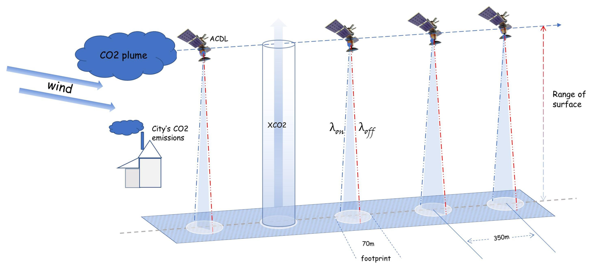
Figure 1 illustrates the detection principle of DQ-1. The XCO₂ products generated by ACDL are similar to those of GOSAT, adopting a point sampling mode. The lidar operates in nadir observation mode, with approximately one 70 m footprint observed every 350 m along the track.

According to Eq. (1), we calculate XCO₂ by directly using the integrated weighting function (IWF). Significant differences in XCO₂ measurements can be observed between ACDL and OCO-2/3. Currently, passive remote sensing satellites like OCO-2/3 and GOSAT estimate XCO₂ by measuring the solar spectrum and using a priori information guided by optimal estimation theory to derive XCO₂(p), ultimately obtaining XCO₂ (Miller et al., 2014). In contrast to these traditional passive optical remote sensing satellites, ACDL does not “estimate” xCO₂(p) but directly “calculates” the weighted average column concentration (Zhang et al., 2024). During the integration phase of ACDL's development, we evaluated the WF (Weighting Function) shapes of various on-line wavelengths and selected one that responds strongly near the surface and weakly at higher altitudes (Han et al., 2025). This design allows changes in surface CO₂ concentration, driven by surface CO₂ fluxes, to be more prominently reflected in the column concentration. Therefore, this WF enhances the ability to identify surface CO₂ variations and provides more information for subsequent CO₂ flux inversion.

Unlike the XCO₂ products from passive satellites such as OCO-2/3, the XCO₂ product from DQ-1 (hereafter referred to as XCO2^Lidar to distinguish it from passive satellite XCO₂ products) is derived using the differential between on-wavelength (strong CO₂ absorption) and off-wavelength (weak CO₂ absorption) measurements. In this context, XCO2^Lidar is obtained through the differential of the lidar signals and integration weighting functions described in Eqs. (1) and (2). Here, WF(p) represents the lidar signal and p represents the pressure:

$$\begin{array}{}\text{(1)}& {\mathrm{XCO}\mathrm{2}}^{\mathrm{Lidar}}=={\displaystyle \frac{\mathrm{2}\cdot \ln \left(\frac{V_{\mathrm{off}}\cdot V_{\mathrm{on}-\mathrm{0}}}{V_{\mathrm{on}}\cdot V_{\mathrm{off}-\mathrm{0}}}\right)}{{\int }_{p\mathrm{\_}\mathrm{surface}}^{p\mathrm{\_}\mathrm{toa}}\mathrm{WF}\left(p\right)\mathrm{d}p}}\end{array}$$

Here, V_on and V_off represent the reflected signal energies at the on-wavelength and off-wavelength, respectively, while V_on−0 and V_off−0 denote the transmitted signal energies. p_surface indicates the atmospheric pressure at the laser ground point, and p_top represents the pressure at the TOA of the atmosphere.

The denominator of Eq. (1) represents the integration weighting function, as detailed in the study by (Refaat et al., 2016):

$$\begin{array}{}\text{(2)}& \mathrm{WF}\left(p\right)=\mathrm{\Delta }{\mathit{\sigma }}_{\mathrm{wf}}\left({\mathit{\lambda }}_{\mathrm{on}}{\mathit{\lambda }}_{\mathrm{off}}p\right)\cdot N_{\mathrm{dry}}\left(p\right)\end{array}$$

Here, $\mathrm{\Delta }{\mathit{\sigma }}_{\mathrm{wf}}({\mathit{\lambda }}_{\mathrm{on}},{\mathit{\lambda }}_{\mathrm{off}},p)$ denote the CO₂ differential absorption cross-sections at the on-wavelength and off-wavelength, respectively. N_dry represents the number of dry air molecules per unit volume in the pressure layer. This formula allows for the construction of the relationship between XCO2^Lidar and the CO₂ profile CO2(p):

$$\begin{array}{}\text{(3)}& \begin{array}{rl}& {\mathrm{XCO}\mathrm{2}}^{\mathrm{Lidar}}={\displaystyle \frac{{\int }_{p\mathrm{\_}\mathrm{surface}}^{p\mathrm{\_}\mathrm{toa}}\mathrm{CO}\mathrm{2}\left(p\right)\mathrm{WF}\left(p\right)}{{\int }_{p\mathrm{\_}\mathrm{surface}}^{p\mathrm{\_}\mathrm{toa}}\mathrm{WF}\left(p\right)\mathrm{d}p}}=\\ & {\displaystyle \frac{\mathrm{WF}\left(p_{\mathrm{1}}\right)}{\mathrm{IWF}}}\cdot \mathrm{CO}\mathrm{2}\left(p_{\mathrm{1}}\right)+{\displaystyle \frac{\mathrm{WF}\left(p_{\mathrm{2}}\right)}{\mathrm{IWF}}}\cdot \mathrm{CO}\mathrm{2}\left(p_{\mathrm{2}}\right)+\mathrm{\cdots }\end{array}\end{array}$$

2.2 Study Area

Considering the available orbital tracks for DQ-1 inversion, vegetation coverage, and the complexity of meteorological conditions, this paper selects three cities and regions to highlight the different sources of uncertainty in emission inversion and the inversion capability of DQ-1. The selected cities share the following characteristics: (1) high fossil fuel emissions; (2) typical “plume cities” (Ye et al., 2020) characterized by ffXCO₂ enhancements distributed in plume forms (Deng et al., 2017). Riyadh, with a population of 8 million, and Cairo, with a population of 20 million, have significantly weaker biosphere contributions compared to Beijing. In subsequent research, it is considered that the spatial gradient of biosphere CO₂ flux can be ignored compared to local fossil fuel emissions.

To assess the impact of biosphere flux uncertainty on the inversion process and separately evaluate the impact of daytime and nighttime biosphere flux on the simulated local XCO₂ enhancement, we selected Beijing, the capital city of China, with a population of approximately 21.5 million. Beijing is not only the political center of China but also one of the most populous cities. Compared to its surrounding areas, Beijing has relatively less vegetation. Surrounding cities might have better-preserved natural ecological environments and more abundant vegetation cover due to less industrialization and urbanization (Che et al., 2022). For instance, the mountainous and suburban areas around Beijing may have more forests, grasslands, and farmlands, whereas green spaces within Beijing are often limited to parks, green belts, and a few nature reserves. As a city with high fossil fuel emissions and active biosphere exchange, Beijing is well-suited for studying the impact of biosphere flux uncertainty on emission estimates.

2.3 Atmospheric Model Setting

2.3.1 WRF-STILT

The spatial heterogeneity of emissions and dense point sources (such as power plants) lead to a complex spatial structure of urban emissions, resulting in intricate ffCO₂ plumes combined with local atmospheric dynamics (Wang et al., 2025). To explore fine-scale urban emission patterns, this study employs the WRF-STILT model (WRF: Weather Research and Forecasting, STILT: Stochastic Time-Inverted Lagrangian Transport). The STILT Lagrangian model driven by WRF meteorological fields is characterized by a realistic treatment of convective fluxes and mass conservation properties, which are crucial for accurate top-down estimates of CO₂ emissions.

In this study's application of STILT, hourly outputs from version 4.0 of WRF are used to provide high-resolution meteorological fields, with the model grid configured to 51 vertical (eta) layers. The 6-hourly NCEP FNL (Final) global operational analysis data with a resolution of 1° are used as initial and boundary conditions for meteorological and land surface fields to provide the initial and boundary conditions for WRF runs. The simulations run for 30 h, but only the 7th to 30th hours of each simulation are used to avoid spin-up effects in the first 6 h.

Each city uses the same one-way WRF nesting at 27, 9, and 3 km resolutions, with Riyadh (23.7625° N, 45.7625° E −25.4375° N, 27.4375° E), Cairo (29.1625° N, 30.4125° E–30.8375° N, 32.0875° E), and Beijing (39.4° N, 115.5° E–41.075° N, 117.175° E) having their innermost regions used to filter DQ-1's orbital data. The study area for STILT is set to be smaller than the innermost WRF region to eliminate the marginal effects of WRF. Footprints quantitatively describe the contribution of surface fluxes from upwind areas to the total mixing ratio at specific measurement locations, with units of mixing ratio per unit flux. The footprint used in lidar satellite inversions is different from that used in general optical satellites, as detailed in Sect. 2.4.1. STILT (In this study, we used the STILT model, version 2, to simulate atmospheric transport processes.) is configured to release 500 particles per receptor each time, with forward dispersion over 24 h. The particle release heights for STILT are set within the range of 50–1000 m, with releases every 50, and 1000–2000 m, with releases every 100 m, the spatial resolution of the STILT simulations is 1 km × 1 km. Generally, as MAXAGL increases from 1 to 2 km, the urban enhancement increases and then stabilizes (Wu et al., 2018).

2.3.2 Inventory of Fossil Fuel Emissions

This article uses The Open-source Data Inventory for Anthropogenic CO₂ (ODIAC) which is a global high-resolution fossil fuel carbon dioxide emissions (ffCO₂) data product (Oda and Maksyutov, 2015). The 2023 version of ODIAC (ODIAC2023, 2000–2022) is based on the Appalachian State University's Carbon Dioxide Information Analysis Center (CDIAC) team's (Gilfillan and Marland, 2021; Hefner et al., 2024) most recent national ffCO₂ estimates (2000–2020). The ODIAC emissions inventory provides 1 km × 1 km global monthly average ffCO₂. The spatial decomposition of emissions is accomplished using a variety of spatial proxy data, such as the geographic location of point sources, satellite observations of night lights, and airplane and ship tracks. Seasonality of emissions was obtained from the CDIAC monthly gridded data product (Andres et al., 2011) and supplemented using the Carbon Monitor product (2020–2022, https://carbonmonitor.org/, last access: 20 October 2025). In this paper, monthly data from ODIAC are time-allocated, and neither the subsequent modeling nor the pseudo-data take into account the daily and weekly time-variation of the ACDL product.

2.3.3 Background XCO₂

To extract the XCO₂ enhancement for DQ-1 inversion, we define XCO₂ enhancement as entirely driven by fossil fuel emissions. A classic method for extracting orbital background concentrations involves selecting another “clean” orbit (minimally influenced by fossil fuel emissions) that is spatially and temporally close, and using averaging or linear regression to approximate a background concentration for the orbit under study. In this study, due to the fine-scale urban area emissions inversion, the study area is small, making it challenging to find another clean orbit for calculating the background concentration.

Previous studies have used inversion methods to derive background concentrations for orbits (Pei et al., 2022), but these typically yield a background concentration for a region. These methods usually produce a value unaffected by geographic location within a small area. However, for each orbit we study, a single, constant background concentration is clearly unreasonable. Therefore, based on previous research, we designed a simple and quick method to extract background concentrations, generating a background line for each orbit of interest.

To derive ffXCO2, which represents the enhancement of XCO2 attributed to fossil fuel emissions, we need to subtract the background XCO2 from the observational data obtained by DQ-1. In the study (Ye et al., 2020), XCO2 is decomposed into two components: XCO2_trend and XCO2_local. Here, XCO2_trend represents the non-local trend, while the standard deviation σ_local of XCO2_local indicates variations at the local scale. We filtered the XCO2 samples with $\mathrm{XCO}\mathrm{2}<{\mathrm{XCO}\mathrm{2}}_{\mathrm{trend}}+\mathrm{0.5}{\mathit{\sigma }}_{\mathrm{local}}$. These filtered data are designated as “background samples” (represented by blue triangles in Figs. 3, 5, 7) due to their lower spatial variability at the local scale compared to samples affected by urban ffCO2 emissions. We then performed linear regression based on the “background samples” to recalculate the linear regression line, referred to as the “background line”. This “background line” method accounts for spatial trends in the background data. Unlike Ye et al. (2020), we utilized the low-frequency (approximate) coefficients obtained from DWT to characterize.

2.3.4 Biogenic Carbon Flux

We specifically considered the influence of biogenic flux on the emission constraints in urban areas for DQ-1. Two open-source NEE datasets were utilized in our study. The first dataset is derived from the Carnegie-Ames-Stanford Approach-Global Fire Emissions Database Version 3 (CASA-GFED3) model (van der Werf et al., 2010), which provides 3-hourly average net ecosystem exchange (NEE) of carbon. This dataset incorporates biogenic fluxes as well as fluxes associated with biomass burning emissions, offering a global coverage of 3-hourly average NEE.

Additionally, we considered the ODIAC dataset, which provides advanced data-driven products on global primary production, net ecosystem exchange, and ecosystem respiration (Zeng, 2020). The ODIAC dataset offers 10 d average global NEE data and utilizes extensive ecosystem indices from MODIS and ERA5 to deliver more precise data.

According to the study by Ye et al. (2020), to better describe the diurnal variations and spatial distribution of biogenic fluxes, the MODIS green vegetation fraction (GVF) was used to downscale the 3-hourly NEE from the original grid resolutions (CASA NEE 0.5° × 0.625° and ODIAC NEE 0.1° × 0.1°) to the WRF domain resolutions (27, 9, and 3 km). This method assumes a linear relationship between carbon uptake and release and the vegetation canopy coverage.

Our application of these datasets and downscaling methods enables a more accurate representation of biogenic flux contributions to urban carbon emissions. By integrating high-resolution biogenic flux data, we can improve the precision of emission inventories and enhance our understanding of urban carbon dynamics. This approach allows us to better inform urban planning and policy-making aimed at reducing carbon footprints and mitigating climate change impacts.

2.4 Emission Optimization Method

2.4.1 X-Stochastic Time-Inverted Lagrangian Transport model (“X-STILT v1”)

XSTILT incorporates satellite profiles and provides comprehensive uncertainty estimates of urban XCO2 enhancements on a per sounding basis (Wu et al., 2018). The simulated enhancement in CO₂ emissions due to fossil fuels, $\mathrm{\Delta }\mathrm{CO}{\mathrm{2}}_{\mathrm{ffCO}\mathrm{2}}\left(p\right)=<\mathrm{ffCO}\mathrm{2},\text{foot}\left(h\right)>$, can be interpolated from the modeling results of CO₂ fluxes and tracer-tagged footprints. Therefore, a relationship between CO₂ fluxes and XCO2^Lidar is established:

$$\begin{array}{}\text{(4)}& \begin{array}{rl}& {\mathrm{XCO}\mathrm{2}}^{\mathrm{Lidar}}-{\mathrm{XCO}\mathrm{2}}_{\mathrm{background}}^{\mathrm{Lidar}}=={\displaystyle \frac{\mathrm{WF}\left(p_{\mathrm{1}}\right)}{\mathrm{IWF}}}\\ & \cdot <\mathrm{ffCO}\mathrm{2},\mathrm{foot}\left(h_{\mathrm{1}}\right)>+{\displaystyle \frac{\mathrm{WF}\left(p_{\mathrm{2}}\right)}{\mathrm{IWF}}}\\ & \cdot <\mathrm{ffCO}\mathrm{2},\mathrm{foot}\left(h_{\mathrm{2}}\right)>+\mathrm{\cdots }\end{array}\end{array}$$

Here, ${\mathrm{XCO}\mathrm{2}}_{\mathrm{ffCO}\mathrm{2},\mathrm{obs}}^{\mathrm{Lidar}}={\mathrm{XCO}\mathrm{2}}^{\mathrm{Lidar}}-{\mathrm{XCO}\mathrm{2}}_{\mathrm{background}}^{\mathrm{Lidar}}$ represents the XCO₂ enhancement extracted from DQ-1 observational data, and ${\mathrm{XCO}\mathrm{2}}_{\mathrm{background}}^{\mathrm{Lidar}}$ represents the background concentration selected from the DQ-1 orbit (detailed in Sect. 2.3.3). The symbol $<,>$ denotes the inner product operator, ffCO2 is the prior emission flux, and foot(h_n) represents the simulated footprints at different altitude layers. This formula establishes the mathematical foundation for inversion.

By integrating footprints from different release heights (Sect. 2.3.1 explains the selection of STILT release heights), we further simplify the above equation. Here, we define ${\mathrm{XCO}\mathrm{2}}_{\mathrm{ffCO}\mathrm{2},\mathrm{sim}}^{\mathrm{Lidar}}$ as the XCO₂ enhancement simulated by the atmospheric transport model.

$$\begin{array}{}\text{(5)}& {\displaystyle }{\mathrm{XCO}\mathrm{2}}_{\mathrm{ffCO}\mathrm{2},\mathrm{sim}}^{\mathrm{Lidar}}=<{\mathrm{XSTILT}}^{\mathrm{Liadr}}\mathrm{ffCO}\text{(6)}& {\displaystyle }{\mathrm{XSTILT}}^{\mathrm{Lidar}}={\sum }_{i=\mathrm{1}}^n{\displaystyle \frac{\mathrm{WF}\left(p_i\right)}{\mathrm{IWF}}}\cdot \mathrm{foot}\left(h_i\right)\end{array}$$

Here, we define XSTILT^Lidar as the column-averaged footprint, corresponding to the column-averaged CO₂ concentration. The inner product of the column-averaged footprint and the prior emission flux yields the simulated XCO₂ enhancement. Thus, we can optimize the fossil fuel CO₂ (ffCO₂) emission parameters using the simulated and observed XCO₂ enhancements to achieve the best consistency between the model and observed increments. By achieving this optimization, we ensure that the model accurately reflects the observed data, providing a reliable basis for further studies and policy-making.

Considering previous studies that used OCO-2/3 and GOSAT for inversion (Patra et al., 2021; Roten et al., 2022; Wang et al., 2019), we selected one of these inversion methods (Ye et al., 2020) for comparison with DQ-1 inversions and validation using TCCON site data (see Sect. 3.2). The posterior scaling factor was applied to the ODIAC inventory flux to simulate XCO₂ at TCCON site locations, and these simulations were compared with TCCON data, assumed to be the true XCO₂ at those locations. ACDL observations require the use of the IWF to derive X-STILT footprints, which differ from those used for TCCON sites. The simulated XCO₂ for TCCON was obtained using an integration method provided by TCCON, with 51 altitude levels corresponding to the input levels of our STILT model. The footprints from these 51 altitude levels were integrated using the integration operator integration_operator_x2019 and the averaging kernel ak_xCO₂ to obtain the simulated XCO₂.

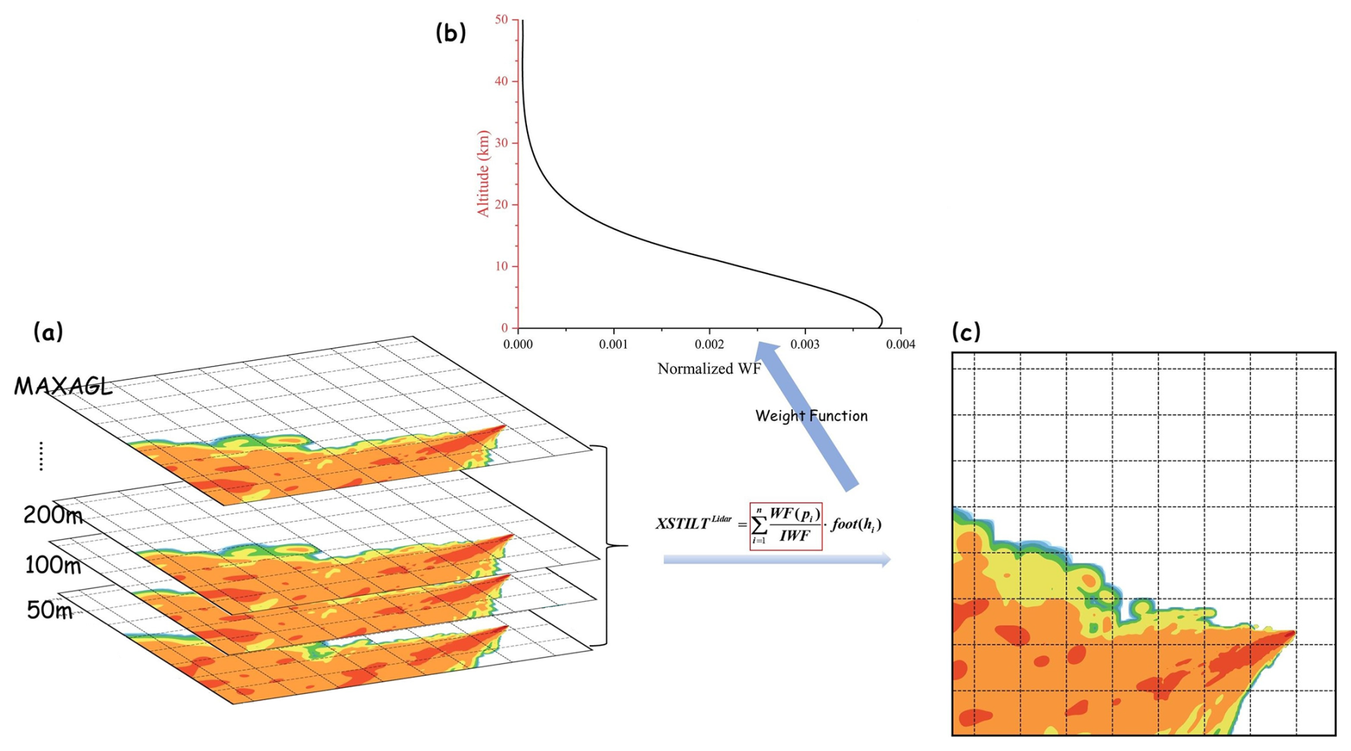
Figure 2 Schematic diagram of XSTILT, (a) represents the simulated footprints at each horizontal altitude level we set (one footprint per 50 m below 1000 m, one footprint per 100 m from 1000–2000 m, where MAXAGL represents the highest atmospheric altitude we simulate, which is 2000 m) and the column average footprints obtained by integrating using the normalized integration function in (b) and (c).

2.4.2 Optimization of Emission Constraint Factors

We adopted a Bayesian inversion method similar to that used by Ye et al. (2020), which utilizes OCO-2 observational data to constrain ffXCO₂, aiming to achieve correlation between the model and observed ffXCO₂ increments. Unlike the inversion of individual emission grids, we optimize emissions by adjusting a scaling factor (λ) for the entire city's prior emissions without modifying each grid's flux individually. The observational data along the DQ-1 orbit across all regions of interest serve as constraints for the inversion, which can be expressed as:

$$\begin{array}{}\text{(7)}& y_{\mathrm{obs}}=y_{\mathrm{sim}}\cdot \mathit{\lambda }+{\mathit{\epsilon }}_{\mathrm{obs}}\end{array}$$

Here, y_obs and y_sim represent the observed and simulated ffXCO₂ enhancements, respectively. The term ε_p denotes the observational error, which consists of DQ-1 measurement error, model error, and model parameter error, defined as follows:

$$\begin{array}{}\text{(8)}& \begin{array}{rl}{y}_{\mathrm{obs}}& =\mathrm{mean}\left(\underset{\text{time1}}{\overset{\text{time2}}{\int }}\mathrm{dXCO}{\mathrm{2}}_{\text{obs}}\mathrm{d}t\right),\\ & y_{\mathrm{sim}}=\mathrm{mean}\left(\underset{\mathrm{time}\mathrm{1}}{\overset{\mathrm{time}\mathrm{2}}{\int }}\mathrm{ffXCO}{\mathrm{2}}_{\mathrm{sim}}\mathrm{d}t\right)\end{array}\end{array}$$

Here, dXCO2_obs represents the DQ-1 XCO₂ enhancement after removing the background concentration. ffXCO2_sim represents the simulated XCO₂ enhancement, obtained from the convolution of the fossil fuel emission inventory and the footprint. We averaged the DQ-1 data over 1 s intervals (7 km) along the orbit to obtain ffXCO2_obs and corresponding simulated data ffXCO2_sim.

According to the Bayesian inversion method, we transform the state vector into a scaling factor (λ), which represents the constraint ability of pseudo-observations on regional emissions. The Jacobian matrix is given by the simulated XCO₂ enhancement y_sim. The observation error variance ${\mathit{\sigma }}_{\mathrm{measurement}}^{\mathrm{2}}$ and model transport error variance ${\mathit{\sigma }}_{\mathrm{mod}}^{\mathrm{2}}$ are considered. We assume that DQ-1 observations are unbiased with respect to the true values. Random errors were added to the observations, following a Gaussian distribution with a standard deviation of 0.5 ppm, representing the lower limit of observational errors.

The transport model error was obtained by perturbing wind speed and wind direction errors; more wind observations help reduce atmospheric transport uncertainties. For example, data assimilation systems have proven useful in reducing atmospheric transport errors in data-rich areas like Los Angeles (Lauvaux et al., 2016). Besides systematic wind direction errors, some areas exhibit positive/negative wind direction biases (Ye et al., 2020). The X-STILT model proposed by Wu et al. (2021) can correct wind biases by rotating model trajectories. the transport model error propagates by transforming the model ffXCO₂ plumes with added random wind speed and wind direction errors (by rotating ffXCO₂ plumes). To estimate transport model uncertainty in the model ffXCO₂, we performed multiple (10⁴ times) random wind speed and direction perturbations on the model plume and extracted the uncertainty distribution of ffXCO₂ using the 25th and 75th percentiles. We establish the loss function J(x) to calculate the posterior scaling factor:

$$\begin{array}{}\text{(9)}& {\displaystyle }\begin{array}{rl}J\left(\mathit{\lambda }\right)& =(y_{\mathrm{obs}}-y_{\mathrm{sim}}\mathit{\lambda }{)}^T{\mathbf{S}}_{\mathrm{obs}}^{-\mathrm{1}}(y_{\mathrm{obs}}-y_{\mathrm{sim}}\mathit{\lambda })\\ & +(\mathit{\lambda }-{\mathit{\lambda }}_a{)}^{\mathrm{2}}{\mathit{\sigma }}_{\mathrm{sim}}^{-\mathrm{2}}\end{array}\text{(10)}& {\displaystyle }{\mathit{\sigma }}_{\mathrm{obs}}^{\mathrm{2}}={\mathit{\sigma }}_{\mathrm{measurement}}^{\mathrm{2}}+{\mathit{\sigma }}_{\mathrm{mod}}^{\mathrm{2}}\end{array}$$

Here, S_obs represents the observational error covariance matrix. We assume that the observational errors of different orbits are uncorrelated, so S_obs is a diagonal matrix with the observational error variances ${\mathit{\sigma }}_{\mathrm{obs}}^{\mathrm{2}}$ on the main diagonal. Since the DQ-1 measurement errors and atmospheric transport model errors are unbiased and uncorrelated, we estimate ${\mathit{\sigma }}_{\mathrm{obs}}^{\mathrm{2}}$ by summing both error variances. λ_a represents the prior value of the scaling factor, uniformly set to 1. σ_sim represents the uncertainty of prior emissions, derived from previous studies combined with the emission characteristics of different cities. Since the ODIAC product does not provide uncertainty estimates, ODIAC was originally designed for atmospheric CO₂ flux calculations to reduce model biases caused by coarse grid resolution. Considering the simple downscaling based on nightlights in ODIAC, urban emissions derived from ODIAC are affected by errors related to emission disaggregation. For example, Lauvaux et al. (2016) reported a 20 % difference compared to Gurney et al. (2012) despite significant differences in emission modeling methods. Gurney et al. (2019) further compared the ODIAC and Hestia products for four US cities (Los Angeles, Salt Lake City, Indianapolis, and Baltimore), finding city-wide emission differences ranging from −1.5 % (Los Angeles) to 20.8 % (Salt Lake City). Empirical values of ODIAC ffCO₂ uncertainty can be obtained by comparing ODIAC inventories with other emission fluxes, such as those created using high-resolution top-down satellite products. Smaller temporal scales result in greater empirical value deviations. Considering different city emission characteristics, such as industrial cities like Cairo and Riyadh with irregular emissions and large uncertainties in industrial emissions, we set prior emission uncertainties for these cities at 45 %. For large cities with distinct and regular emission characteristics, the uncertainty is set at 25 %, as their emission estimates are more accurate compared to industrial cities.

By minimizing the loss function, we obtain the posterior scaling factor $\stackrel{\wedge }{\mathit{\lambda }}$ and posterior uncertainty:

$$\begin{array}{}\text{(11)}& {\displaystyle }={\mathit{\lambda }}_a+{\mathit{\sigma }}_{\mathrm{sim}}^{\mathrm{2}}{y}_{\mathrm{sim}}^T(y_{\mathrm{sim}}{S}_{\mathrm{obs}}{y}_{\mathrm{sim}}^T+S_{\mathrm{obs}}{)}^{-\mathrm{1}}(y_{\mathrm{obs}}-y_{\mathrm{sim}}{\mathit{\lambda }}_a)\text{(12)}& {\displaystyle }=(y_{\mathrm{sim}}^T{S}_{\mathrm{obs}}^{-\mathrm{1}}{y}_{\mathrm{sim}}+{\mathit{\sigma }}_{\mathrm{sim}}^{-\mathrm{2}}{)}^{-\mathrm{1}}\end{array}$$

To evaluate the performance of the scaling factor, we define the mean kernel ($\mathrm{AK}=\partial /\partial \mathit{\lambda }$):

$$\begin{array}{}\text{(13)}& \mathrm{AK}=(y_{\mathrm{sim}}^T{S}_{\mathrm{obs}}^{-\mathrm{1}}{y}_{\mathrm{sim}}+{\mathit{\sigma }}_{\mathrm{sim}}^{-\mathrm{2}}{)}^{-\mathrm{1}}(y_{\mathrm{sim}}^T{S}_{\mathrm{obs}}^{-\mathrm{1}}{y}_{\mathrm{sim}})\end{array}$$

The value of AK closer to 1 indicates a more accurate estimation of the scaling factor.

2.5 OSSEs: Optimization of Emissions using Different DQ-1 Tracks

Given the limited number of DQ-1 overpass tracks and the impact of atmospheric conditions during overpasses on emission optimization, we implemented Observing System Simulation Experiments (OSSEs). These experiments were conducted using multiple DQ-1 tracks to constrain urban fossil fuel emissions repeatedly and to statistically evaluate DQ-1's potential in constraining urban fossil fuel emissions. Specifically, we initially screened all DQ-1 overpass tracks, selecting those located downwind of major fossil fuel emission areas to better utilize DQ-1 data for constraining overall regional fossil fuel emissions. For each city's overpass track, we extracted pseudo-observation data and modeling data.

DQ-1 is different from other passive remote sensing satellites in that it is not only capable of night observation, but also less affected by clouds and aerosols. Therefore, we studied the relationship between daytime and nighttime observations and emission estimation uncertainties, as well as the impact of different tracks and the number of tracks on emission estimates. We used the ODIAC fossil fuel emission inventory as the prior emissions for the OSSEs, assuming that the prior emissions are the true emissions and that emissions remain stable over a short period. It is noteworthy that, in Sect. 3.3, the prior emissions were constructed by combining ODIAC fossil fuel data with NEE (Net Ecosystem Exchange).

Pseudo-observation data and modeling data for each city were derived using the same method. Pseudo-observation data were obtained by averaging the 1 s detection range of the selected DQ-1 overpass tracks, with adjacent pseudo-observation data separated by 7 km (1 s). This method helps eliminate some of the background noise and wind speed impacts on emission optimization. We assumed that DQ-1 observations are unbiased with respect to the true values and added random errors to each DQ-1 observation, with the error following a Gaussian distribution and a standard deviation of 0.5 ppm. Pseudo-observation data are also unbiased relative to the true values, with random errors accumulated over time for each observation data: $\mathit{\sigma }\left(\mathrm{1}\mathrm{s}\right)=\sqrt{\frac{{\sum }_{i=\mathrm{1}}^N{\mathit{\sigma }}_{i,\text{DQ-1}}^{\mathrm{2}}}{N^{\mathrm{2}}}}$ Here, σ represents the random error of each pseudo-observation data. Modeling data were obtained by convolving the emission inventory of the area with the tracer contributions corresponding to the geographic locations.

By using multiple DQ-1 overpass tracks to repeatedly constrain urban fossil fuel emissions and analyzing the results statistically, we assessed the potential of DQ-1 in constraining fossil fuel emissions in urban areas. This approach allowed us to examine the effectiveness of daytime and nighttime observations, the influence of different overpass tracks, and the impact of track quantity on emission estimates.

3 Results

3.1 Fossil Fuel Enhancement in Urban Areas

In this section, we summarize the prior ffXCO₂ emissions for each study area. The total monthly emissions for Beijing, Riyadh, and Cairo during the selected months (The detailed overpass dates are emissions provided in Table S3) are approximately 2.4–3.5, 2.3–3.3, and 1.9–2.4 Mt C/month, respectively. We constrain emissions by comparing observed and simulated ffXCO₂ enhancements. Here, ffXCO₂ enhancement is defined as the increment in XCO₂ concentration caused by local fossil fuel emissions. The prior ffXCO₂ enhancement is simulated using the ODIAC prior emission inventory and the STILT footprint (a summed 24 h column integrated footprint) convolution. The observed ffXCO₂ enhancement from DQ-1 is obtained by subtracting the background concentration from the observational data (as detailed in Sect. 2.3.3 and shown in Fig. 3). By comparing the prior ffXCO₂ enhancement with the observed XCO₂ enhancement, we evaluate the trends in ffXCO₂ changes along the tracks and explore the sources and detection capabilities of the ffXCO₂ signal.

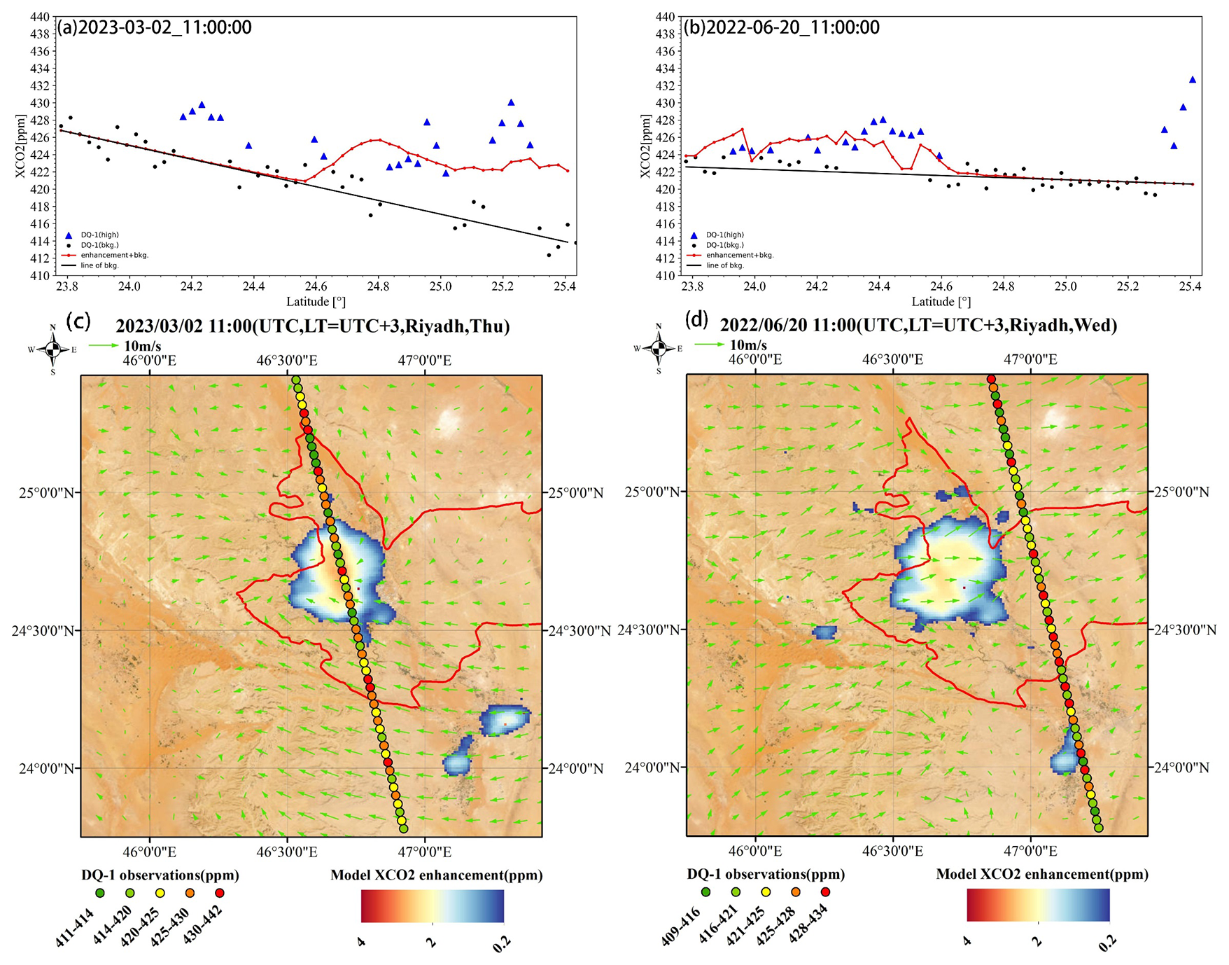
Figure 3 Comparison of the simulated and observed ffXCO₂ enhancements from DQ-1 data over Riyadh on 2 March 2023 and 20 June 2022 around 11:00 UTC. Panels (a) and (b) show the DQ-1 XCO₂ (black dots and blue triangles) and the simulated XCO₂ (red solid line, sum of simulated ffXCO₂ and background concentrations) along the two orbits, averaged over 1 s. The black dots represent the background concentrations involved in deriving the background. The black dots represent the data involved in the derivation of the background concentration (black solid line), which are linearly regressed against latitude after a discrete wavelet transform. Panels (c) and (d) show the simulated ffXCO₂ and the observed ffXCO₂ obtained from the DQ-1 data. background XCO₂ concentrations have been subtracted. The red boxes in the panels (c) and (d) represent the urban areas. Vectors represent 10 m wind speeds (average wind speed simulated by WRF) and reference vectors represent 10 m s⁻¹ wind speeds.

Figure 3 presents the results of two DQ-1 overpasses over Riyadh on 2 March 2023, and 20 June 2022, at 11:00 a.m. Figure 3a and b show the simulated and the observed XCO₂ enhancement as a function of latitude for these two overpasses. The maximum ffXCO₂ enhancements observed along the two tracks were 8 and 5 ppm, respectively.

In the overpass on 2 March, significant ffXCO₂ enhancements were observed by DQ-1 between 24.8 and 25.3° N, with the simulated ffXCO₂ also responding to this enhancement. Although the peak observed values were narrower than the simulated values, both were of similar magnitudes, with only slight differences, and their trends were largely consistent. However, the simulated ffXCO₂ did not respond to the observed enhancement in the 24.1 to 24.3° N range, which may be due to the sensitivity of the STILT footprint to wind direction.

Compared to the track on 2 March, the track on 20 June shows better agreement between observations and simulations, along with smaller posterior uncertainties (see Table 1). The observed peak and the simulated peak were both within the 23.8 to 24.6° N range, with a difference of less than 1 ppm. The differences between the results of the two tracks may be because the 2 March track passed through the city's main emission area and intersected the simulated plume (Fig. 3c). In this case, the observed ffXCO₂ fluctuations were minimal, with values remaining high relative to the background concentration, making it difficult to detect significant enhancements. In contrast, the 20 June track was downwind of the main emission area, making it more sensitive to the city's fossil fuel emissions and resulting in better agreement between the simulated and observed values.

For Cairo, we examined ffXCO₂ enhancements using six DQ-1 overpasses on 26 July, 2 August, 16 August, 8 November, 15 November, and 22 November 2022 (Figs. S9–S10 in the Supplement). In contrast to Riyadh, the simulated ffXCO₂ enhancements over Cairo were mostly below 2 ppm, indicating lower overall emissions in Cairo than in Riyadh. The simulated ffXCO₂ enhancements over Cairo were more dispersed, showing a multi-point distribution rather than the concentrated enhancements observed over Riyadh.

The observed XCO₂ enhancement over Cairo were generally higher and narrower than the simulated ones, which were smoother. Despite these differences, the trends in ffXCO₂ enhancements between the simulations and observations were similar and of the same magnitude (The latitudinal distribution and magnitude of the simulated enhancement (red line) are generally consistent with those of the observed enhancement (blue triangles)), except for the 26 July simulation, which did not include some observed enhancements between 30.2 and 30.4° N, and the 8 November overpass, where a spatial shift of approximately 0.2° was observed between the simulated and observed ffXCO₂ enhancements.

Overall, the comparison between DQ-1 observations and WRF-STILT-based simulations suggests that the DQ-1 satellite is well-suited for fine-scale urban emission optimization. This indicates that DQ-1 can effectively be used for detailed monitoring and analysis of urban emissions.

3.2 Comparison of DQ-1 and OCO-2 Restraint Capabilities

To better compare the inversion results from OCO-2 and DQ-1, we selected tracks that were spatially and temporally close and located downwind of major urban emission areas. Figure 4 shows two pairs of OCO-2 and DQ-1 tracks over Beijing on 1 December 2022, and 8 April 2023, both at 05:00 UTC, passing through the major emission downwind area of the city. Figure 5 shows ffXCO₂ enhancements and wind fields at the time of the satellite overpasses. The results clearly indicate significant ffXCO₂ enhancements, exceeding 2 ppm in April, demonstrating that DQ-1 can observe notable ffXCO₂ enhancements from space.

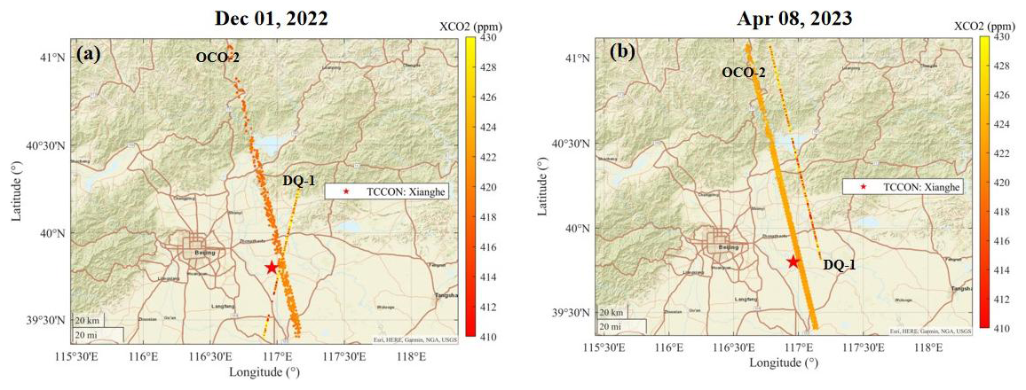
Figure 4 (a) and (b) show the position and XCO₂ data of two pairs of OCO-2 and DQ-1 orbits that we selected for transit to Beijing at 05:00 UTC on 1 December 2022 and 05:00 on 8 April 2023, respectively.

Figure 5c, d, g, h show that the ffXCO₂ enhancements simulated from DQ-1 and OCO-2 overpasses are of similar magnitude and spatial distribution, with strong spatial consistency across different times due to stable local emissions and wind fields. Beijing's topography, with high elevations in the northwest and low-lying plains in the southeast, influences the prevailing west-to-east winds, and the flat terrain of the main urban area means the simulated ffXCO₂ is minimally affected by topography. The smaller ffXCO₂ enhancements observed on 1 December compared to 8 April are primarily due to wind directions affecting the track within the 40.2–41° range, making it difficult to simulate emissions.

This comparison highlights the capability of DQ-1 to effectively observe and simulate urban ffXCO₂ enhancements, supporting its application in fine-scale emission optimization.

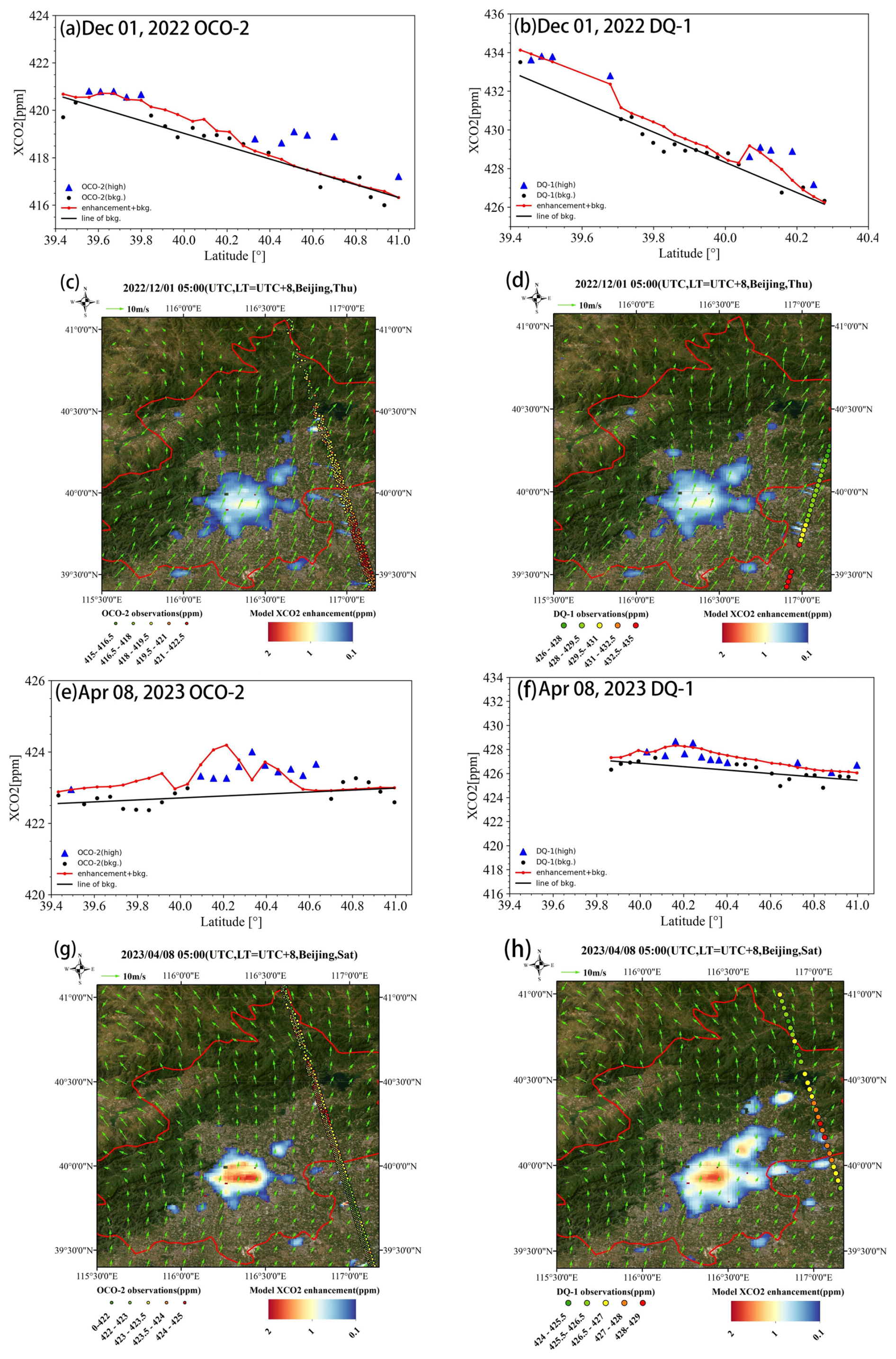
Figure 5 Similar to Fig. 3, (a)–(d) show the simulated ffXCO₂ and measured ffXCO₂ for the DQ-1 and OCO-2 orbits transiting Beijing at 05:00 UTC 1 December 2022 and 05:00 UTC 8 April 2023, and (e)–(h) represent the comparison of the simulated ffXCO₂ (colored shadows) with the observed ffXCO₂ enhancement (colored dots, minus background concentrations) from DQ-1 data collected over Beijing at ∼ 05:00 UTC. Each panel is labeled with the date of observation. The red boxes in the panels (c), (d), (g), (h) represent the urban areas. Vectors represent 10 m wind speeds and reference vectors represent 10 m s⁻¹ wind speeds.

Figure 5a, b, e, f illustrates the simulated and observed XCO₂ for two pairs of DQ-1 and OCO-2 tracks. The simulated XCO₂ (red line in the figures) is derived by adding the background concentration to the simulated ffXCO₂ extracted along the satellite tracks. Overall, both OCO-2 and DQ-1 observations exhibit similar distributions, with high-value points located in the same latitude ranges (On 1 December, both the DQ-1 and OCO-2 overpasses exhibited similarly strong latitudinal gradients in their background baselines, with notable enhancements observed and simulated within the 39.4–39.6° N range. Although the background latitudinal gradients differed between DQ-1 and OCO-2 on 8 April, both were weak in magnitude, and significant enhancements were nevertheless consistently detected and simulated between 40.0 and 40.4° N). DQ-1 observations are generally 4–8 ppm higher than OCO-2, attributed to the inherent characteristics of the satellites – DQ-1 being an active lidar satellite, largely unaffected by clouds and aerosols. This systematic difference can be mitigated during background concentration extraction due to the overall similarity in data distribution.

On 1 December and 8 April, DQ-1 and OCO-2 observed ffXCO₂ enhancements of approximately ∼ 2.5 ppm and ∼ 1.5 ppm, respectively. Although OCO-2 did not capture the ffXCO₂ enhancement within the 40.2–41° range on 1 December, and there was a ∼ 0.15° spatial shift between observed and simulated XCO₂ peaks on 8 April, the simulated ffXCO₂ was of the same magnitude as the observations. This indicates that DQ-1 performs comparably to OCO-2 in urban-scale inversions. The peak shift in OCO-2 data might be due to errors in the horizontal wind field. The background gradient on 1 December was more pronounced than on 8 April, and the integrated ffXCO₂ enhancement along the track was consistent with DQ-1 measurements, validating the latitude gradient-based background extraction method for urban-scale inversions.

Figure 6 compares TCCON site observations within the Beijing study area with the simulated results for 1 December and 8 April. The prior ffXCO₂ (blue bars) represents the simulated ffXCO₂ at the TCCON site, obtained using the previously described simulation method. The posterior ffXCO₂ (light green and orange bars) is derived by applying the posterior scaling factors from DQ-1 and OCO-2 overpass tracks to the prior ffXCO₂, with posterior uncertainties indicated. The true value, provided by TCCON products, is shown by the dark green bars.

Overall, DQ-1 and OCO-2 inversion results are similar in magnitude, with DQ-1 results closer to TCCON observations. The differences between DQ-1 results and TCCON observations are 0.9 % and 16 % for 1 December and 8 April, respectively, compared to 10 % and 25 % for OCO-2. This demonstrates that DQ-1 can effectively constrain urban fossil fuel emissions, performing comparably to, or even surpassing, OCO-2 in certain tracks.

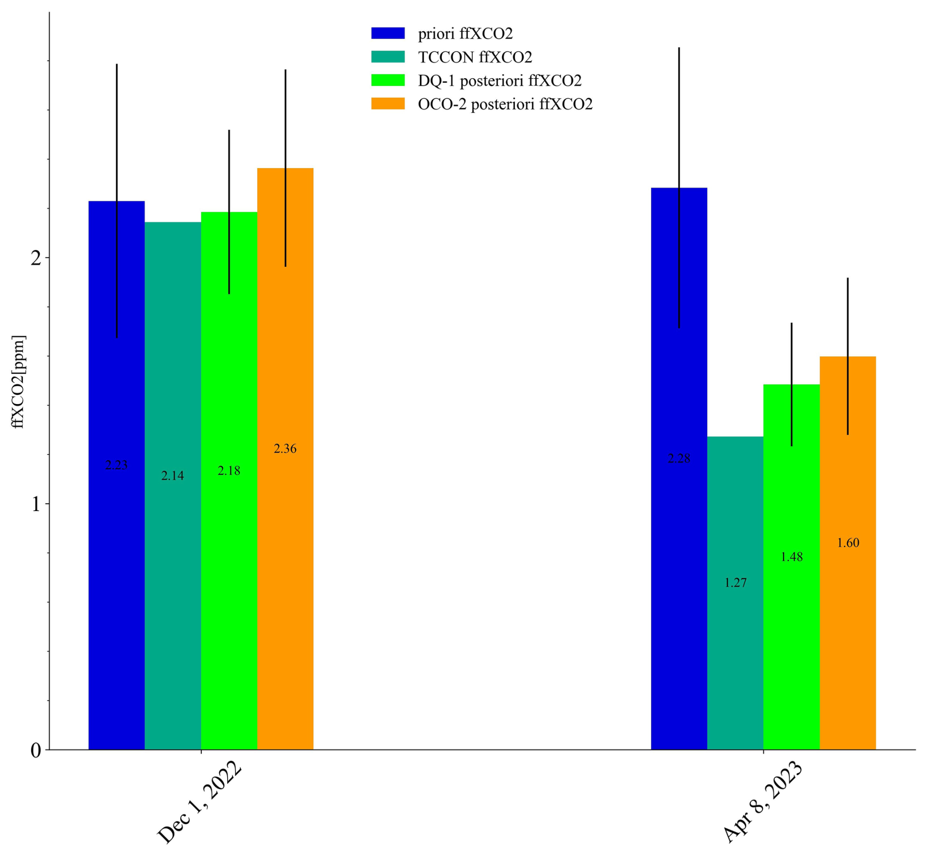
Figure 6 TCCON site simulations received ffXCO₂ (blue columns represent simulations using a priori ODIAC lists, bright green columns represent simulations using a posteriori lists estimated with DQ-1, orange columns represent simulations using a posteriori lists estimated with OCO-2, and dark green columns represent ffXCO₂ observed by TCCON). The black lines on the columns represent uncertainties.

3.3 Impact of DQ-1 in Estimating Biotic Fluxes using Daytime vs. Nighttime Tracks

Both biosphere carbon flux and fossil fuel emissions influence XCO₂ variations. This section examines the impact of biosphere flux on emission estimates. When ffXCO₂ significantly exceeds biosphere carbon flux, the biosphere's contribution to XCO₂ changes can be negligible (e.g., in Cairo and Riyadh, where the spatial gradient of NEE is much smaller than fossil fuel emissions). This study attributes biosphere carbon flux to vegetation production and human emissions. This part of carbon emissions varies with the day-night cycle. During the day, vegetation absorbs CO₂ through photosynthesis, which significantly outweighs CO₂ release through respiration. At night, vegetation only undergoes respiration, releasing CO₂.

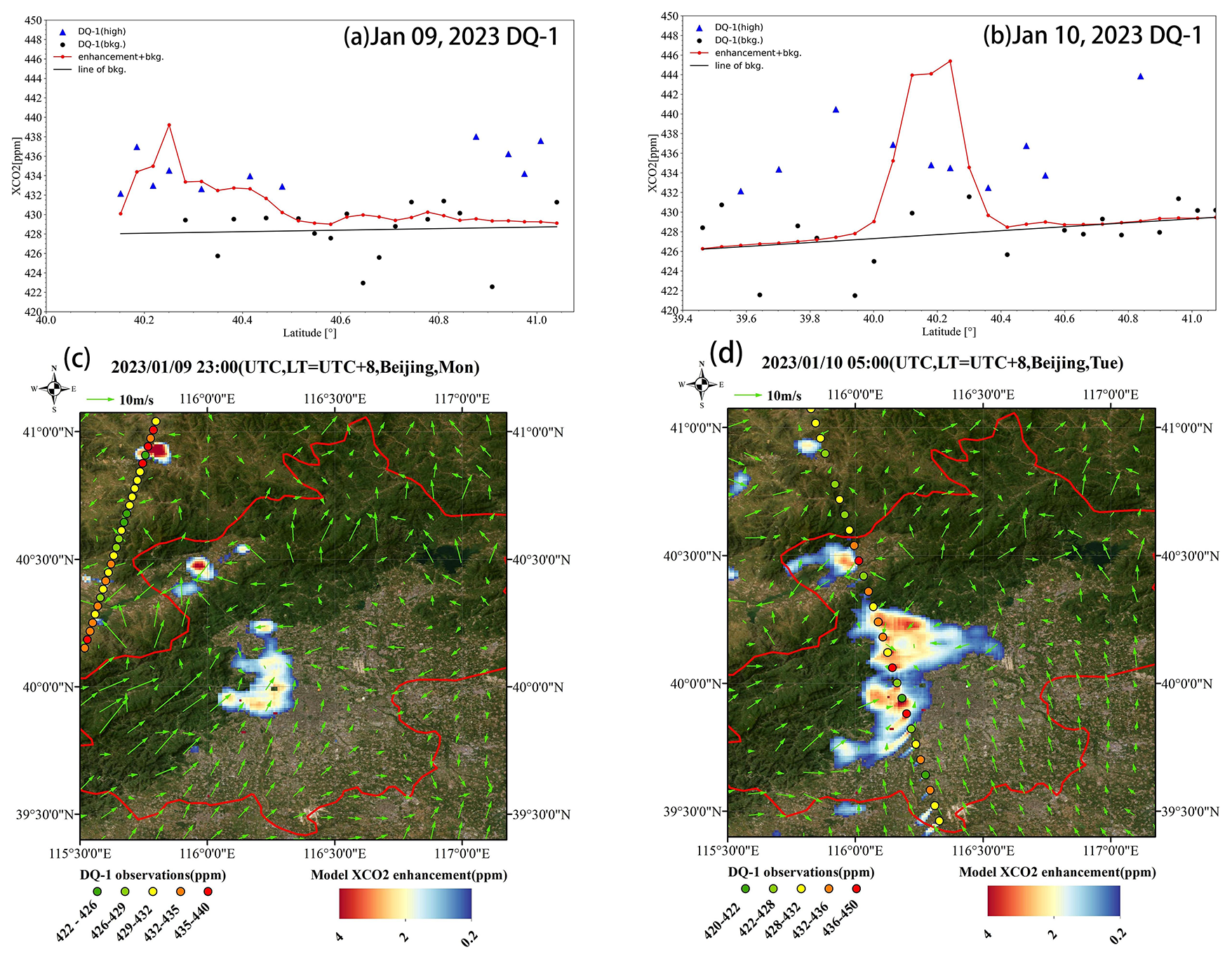
Figure 7 Orbital simulation results for a pair of diurnal observations of the transit of Beijing on 9 January 2023 at about 23:00 (night) and 10 January 2023 at about 11:00 (day) UTC. The red boxes in the panels (c) and (d) represent the urban areas.

As the world's first lidar satellite capable of observing XCO₂ at night, DQ-1 offers groundbreaking potential in studying diurnal variations in urban emissions. This section leverages this feature to observe the impact of vegetation rhythm and human activities on XCO₂ changes. We compare global three-hourly CASA data and ten-day average NEE data from ODIAC. ODIAC's ten-day average data cannot separate diurnal NEE variations, while the higher temporal resolution of CASA can effectively capture the time gradient of NEE within the same day. We will illustrate the impact of NEE on inversion and how this impact changes between day and night. Previous satellite-based urban flux inversions lacked night-time data, preventing day-night comparisons and separation of nocturnal and diurnal CO₂ emissions.

For this study, we selected two tracks on 9 January 2023, at 23:00 and 10 January 2023, at 11:00 (UTC). Given the close timing of these tracks, we assume the total fossil fuel emissions are the same for both. The 9 January track is approximately 0.5° (about 50 km) downwind from the main urban emissions, with an average wind speed greater than 3 m s⁻¹. Thus, the emissions detected by this track are considered to originate from the previous five hours. The 10 January track passes through the main urban emission area, capturing emissions effectively. We simulate the previous 8 h gas diffusion before the overflight (sunset on 9 January at 09:00 and sunrise on 10 January at 15:35 UTC). The simulated enhancement for the 9 January track is assumed to come entirely from night-time emissions, while the 10 January enhancement comes from daytime emissions. Comparing the simulation results with observations, both are of the same magnitude, indicating that the forward eight-hour simulation effectively captures the observed ffXCO₂ enhancement.

To explore the impact of diurnal biosphere carbon flux on XCO₂ enhancement, we couple prior emissions from ODIAC with spatially scaled NEE data as the new prior emissions (For the three-hourly NEE data, we matched using footprints within the corresponding time period), then simulate the XCO₂ enhancement (In contrast to Sect. 3.1 and 3.2, here we used ODIAC emissions combined with NEE as the prior flux information). Using constant boundary conditions, latitude changes do not need to be considered for background concentration. Therefore, local XCO₂ enhancement is defined as the total XCO₂ minus the minimum XCO₂ value in the track (Unlike Sect. 2.3.3). The XCO₂ enhancement measured by DQ-1 is derived using methods outlined in previous sections.

This approach allows us to accurately account for both daytime and nighttime variations in XCO₂ due to biosphere activity, providing a comprehensive view of the urban carbon flux.

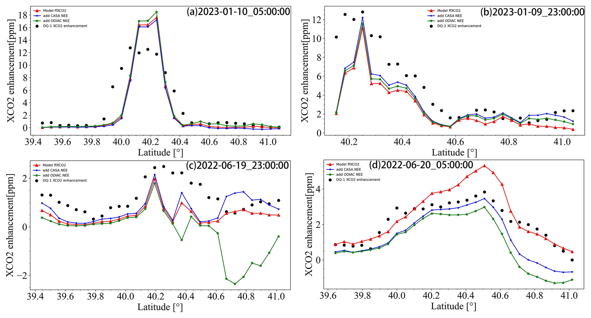
Figure 8 (a)–(d) represent the contribution of orbital XCO₂ enhancement and biospheric fluxes to the local XCO₂ enhancement for two pairs of diurnal observations on 9 and 10 January 2023 and 19 and 20 June 2022, the black dots represent the 1 s averaged observations (subtracted from the background values) on each orbit, the red solid line represents the simulated ffXCO₂, and the green and blue solid lines represent the simulated ΔXCO₂ (fossil fuel and biosphere fluxes) using different NEE data for simulated ΔXCO₂ (fossil fuel and biogenic fluxes), where the green line uses ten-day averaged ODIAC NEE data and the blue line uses CASA three-hourly NEE data.

Figure 8 presents a comparison of simulated and observed XCO₂ enhancements for two pairs of day and night overpass tracks over Beijing on 9 January 2023, at 23:00, 10 January at 05:00, 19 June 2022, at 23:00, and 20 June at 05:00. Overall, the simulated XCO₂ enhancements that include CASA NEE (blue line) on 10 January, 20 June, and 19 June, show better agreement with the observed ΔXCO₂ (black dots) than simulations driven by fossil fuel emissions alone (red line).

The Fig. 8c shows that the XCO₂ enhancements using CASA's diurnal NEE data differ significantly from those using ODIAC's ten-day average NEE data. The simulation for the 19 June track at 23:00 indicates that using CASA's night-time NEE data (blue line) can accurately simulate the observed XCO₂ enhancement, coming closer to the observed XCO₂ enhancement than the ffXCO₂ simulation alone. In contrast, the simulation using ODIAC's ten-day average NEE data (green line) shows a notable CO₂ uptake in the 40.2–41° range, starkly different from the CASA results and the observed XCO₂ enhancement. This discrepancy arises because ODIAC's ten-day average NEE data are insensitive to short-term temporal variations and cannot reflect diurnal changes within a day. Moreover, this period is Beijing's summer, with vigorous daytime vegetation activity leading to CO₂ uptake and a consequent drop in XCO₂ (as seen in Fig. 8d, where the daytime simulated XCO₂ enhancement is much lower than ffXCO₂). According to the 19 June simulation results, biosphere flux-induced XCO₂ changes account for 21.2 % (CASA) and −54.3 % (ODIAC) of the observed XCO₂ enhancement.

For the 9 January track at 23:00, both CASA and ODIAC data show significant XCO₂ enhancements. However, the CASA simulation aligns more closely with the observations. This difference may be because ODIAC's ten-day average data, influenced by daytime data, diminish its accuracy in night-time scenarios. The simulation results for the 9 January track show that biosphere flux-induced local XCO₂ enhancements account for 13.37 % (CASA) and 7.73 % (ODIAC) of the observed comprehensive XCO₂ enhancement.

Overall, the biosphere flux's impact on XCO₂ enhancement varies significantly between day and night. In urban-scale inversions, DQ-1's ability to rapidly revisit both day and night can further optimize the influence of biosphere flux on inversion accuracy. This capability highlights DQ-1's potential to provide more precise urban-scale fossil fuel emission constraints, especially by distinguishing diurnal variations in biosphere activity.

3.4 Emission Estimates and a Posteriori Uncertainties

Table 1 Results of inversion of urban emission scaling factors for selected cities using DQ-1 XCO₂ data.

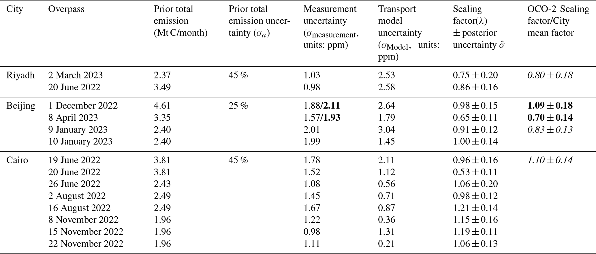
Notes. Scaling factors and their a posteriori uncertainties are shown for each orbit, as well as integrated information for all selected orbits. Uncertainty components are listed for each track, including the a priori uncertainty in the scaling factor and the measurement and transport uncertainty in the integral ffXCO2 (some specific track data inverted using OCO-2 data are bolded, and the average emission scaling factor and a posteriori uncertainty for all tracks in each city are in the last column and highlighted in italics).

In this section, we present the inversion estimation results for emissions from Riyadh, Cairo, and Beijing using the DQ-1 tracks shown in Sect. 3.1. The inversion process considers uncertainties arising from both measurement and transport. The inversion yields a scaling factor for the total emissions for each selected city. Specifically, for Beijing, we compare the inversion results with the simultaneously passing OCO-2 tracks.

Each selected track underwent inversion. Table 1 shows the posterior emission scaling factors for each track, along with the uncertainties in the measured and simulated ffXCO₂. These uncertainties were determined using the methods described in Sect. 2.4. Notably, the prior uncertainty in the emission scaling factors for Beijing was set at 25 %, compared to Riyadh and Cairo, reflecting better knowledge of emissions from such a well characterized megacity (see Sect. 2.4.2).

For the selected tracks over Riyadh, Cairo, and Beijing, the posterior scaling factors (An emission factor greater than 1 indicates an underestimation by the prior inventory, while a factor less than 1 suggests an overestimation.) were 0.75–0.86, 0.98–1.21, and 0.53–1.06, respectively (Table 1). The posterior emission scaling factors exhibit significant temporal variability, influenced by background conditions. As described in the previous section, the emissions detected by the track depend on its distance from the major emission regions and the domain-averaged wind speed at the time. The domain-averaged wind speed for the selected tracks was consistently above 3 m s⁻¹. Based on meteorological conditions, the posterior values represent estimates of city emissions for the hours preceding the overpass time. The posterior uncertainty in the emission scaling factors was 0.16–0.20 for Riyadh, 0.11–0.20 for Cairo, and 0.11–0.16 for Beijing. Compared to Beijing, the posterior scaling factor uncertainties were generally higher for Riyadh and Cairo.

As discussed in Sect. 2.4, the prior emission uncertainties were set to reflect measurement and transport errors. Table 1 shows that the relative contributions of observation error and transport error vary across the three cities. For Riyadh, the transport error was significantly larger than the observation error, while for Cairo, the transport error was much smaller than the observation error. In Beijing, the relative sizes of transport error and observation error varied. The posterior scaling factors for Beijing's two OCO-2 tracks were almost identical to those from DQ-1, with higher posterior uncertainty due to higher observation error. Overall, Beijing's posterior uncertainty was lower than that of Cairo and Riyadh, attributable to more stable prior emission characteristics.

Previous research (Ye et al., 2020) highlighted that the scarcity of OCO-2 tracks near many cities remains a major limitation in regularly quantifying emissions and objectively tracking temporal variations from space. In contrast, DQ-1's minimal sensitivity to clouds and aerosols allows for more tracks available for inversion. Our experiments in Beijing, Cairo, and Riyadh found that, on average, more than six tracks per month were available for inversion, including day and night overpasses on the same day, further constraining city emissions (see Sect. 3.3).

Based on the results in Table 1, we averaged the posterior emission scaling factors and uncertainties for each city's tracks, yielding mean scaling factors and uncertainties of 0.80 ± 0.18 for Riyadh, 1.10 ± 0.14 for Cairo, and 0.83 ± 0.13 for Beijing (Detailed monthly emission information for different cities is provided in Table S3). This indicates that, for the periods represented by the observations, the prior monthly ODIAC product overestimates emissions for Beijing and Riyadh, while underestimating emissions for Cairo, Our findings in Cairo are consistent with earlier research (Shekhar et al., 2020).

4 Discussion

4.1 Atmospheric Transport Model Errors

Systematic errors in model transport and erroneous statistical assumptions can significantly diminish the improvements in land-based uncertainty by approximately a factor of two (Wang et al., 2014). Hence, it is essential to control systematic errors and inaccuracies in transport models while minimizing random errors in DQ-1 observations. In Observing System Simulation Experiments (OSSEs), we assess the potential impacts of observational and transport errors on the entire inversion process. Transport errors of tracers in the atmosphere can lead to inaccuracies in flux estimates derived from concentration observations. Typically, “inversion” methods either ignore transport errors or only provide a rough evaluation of their impact (Lin and Gerbig, 2005). This section focuses on how uncertainties in atmospheric transport model outputs influence CO₂ flux inversion.

In our experiments, we set the prior flux uncertainty to 25 %–45 % based on the emission characteristics of different cities. The uncertainty in DQ-1 XCO₂ observations was fixed at 0.5 ppm, representing the lower limit of observational error. We examined the effects of wind speed and direction errors on the performance of the inversion method. The errors in the transport model were propagated by treating them as conversions of model ffXCO₂ plumes. Notably, for the cities studied, errors were assumed to be unbiased. Wind direction errors were analyzed by rotating the plumes around the emission center and incorporating random wind speed errors.

We illustrate these concepts using six tracks over Cairo. The overall ffXCO₂ distribution was generated by applying random positive and negative wind direction biases ($>-\mathrm{10}$°, <10°) to each track's STILT footprint, rotating it 10⁴ times, and adding positive/negative wind speed biases ($>-\mathrm{1}$ m s⁻¹, < 1 m s⁻¹). Overall, the temporal variability in the posterior emission scaling factors and uncertainties can be attributed to transport model errors. The transport model error significantly influenced the observed ffXCO₂ distribution. Specifically, the track on 15 November was most affected by transport model errors, likely due to its passage through the plume boundary. In contrast, the track on 16 August experienced minimal transport model errors, as it was further from the simulated ffXCO₂ plume, making it less sensitive to small wind direction and speed errors, and The MLH will be higher in summer days and that may reduce the uncertainties for the footprints.

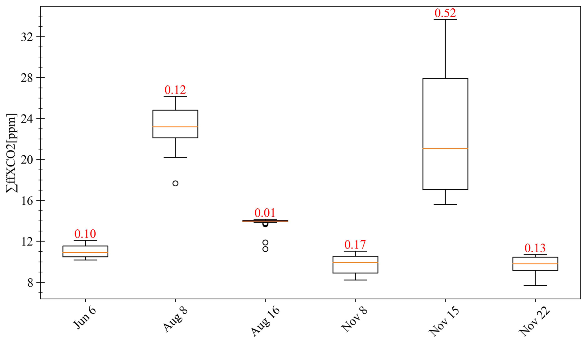
Figure 9 Box plots of the modeled integral ffXCO₂ enhancement (∑ffXCO₂, m) for selected OCO-2 orbits over Cairo at the date labeled on the x-axis (2022). For each box, the center line indicates the median (q2), and the bottom and top edges of the box indicate the 25th and 75th percentiles (q1 and q3), respectively. The whiskers extend to the maximum and minimum values. The numbers are the ratio of the interquartile spacing (q3−q1) to the median (q2).

4.2 The Challenge of Separating Biological Fluxes in Day and Night Orbits

In Sect. 3.3, we detailed how DQ-1's short-term day-night revisit capability allows for the consideration of diurnal and nocturnal biogenic fluxes in emission inversions. Typically, large-scale inversions do not account for uncertainties in fossil fuel emission inventories and treat biogenic fluxes as uncertainties in prior fluxes (Wang et al., 2014). Studies focused on urban-scale inversions that do not utilize nocturnal tracks, while directly considering biogenic flux impacts, have not accounted for the diurnal variation of biogenic fluxes (Ye et al., 2020). In this study, we leveraged DQ-1's nocturnal observations to provide a method for separately considering biogenic flux effects during day and night. Our results indicate that using daytime average NEE data and nighttime NEE data can result in differences of up to 70 % in inversion outcomes.

However, this approach has limitations in large-scale inversions. Separating daytime and nighttime emissions necessitates a limited transport time due to the constraints of the transport model, which means that simulated particles cannot travel long distances under limited wind speed and time conditions. To address this, more frequent overpass tracks, including those from geostationary carbon cycle observation satellites such as GeoCarb (Moore et al., 2018), Total Carbon Column Observing Network (TCCON) (Toon et al., 2009), and MicroCARB, but these instruments are all limited to daylight observations and therefore cannot support day–night inversion analyses, only DQ-1 is capable of enabling such studies. Therefore, an increased availability of high-precision and high-spatial-resolution nighttime data is urgently needed. Currently, the number of DQ-1 tracks does not support large-scale separate day-night inversions. In large-scale flux inversions, biogenic fluxes are typically used as prior uncertainty over weekly or monthly periods. Such long-term and wide-scale data assimilation reduces the impact of diurnal biogenic flux variations on inversion results. Unlike other satellite measurements that are restricted to daytime clear-sky conditions, DQ-1's XCO₂ measurements provide uniform temporal sampling, thus allowing effective quantification of diurnal variations in emissions.

Accurate downscaling methods for biogenic fluxes, such as the Solar-Induced Fluorescence Model (SMUrF) (Wu et al., 2021), and advanced vegetation models, like the Vegetation Photosynthesis and Respiration Model (VPRM) (Luo et al., 2022; Mahadevan et al., 2008; Wei et al., 2022; Winbourne et al., 2022; Gourdji et al., 2022; Yang et al., 2024) are crucial for precise biogenic flux calculations. Radiocarbon and land surface solar-induced fluorescence (SIF) data aid in distinguishing between fossil fuel CO₂ and biogenic CO₂ (Fischer et al., 2017). Recent research indicates that SIF serves as a better indicator or proxy for gross or net primary production compared to other vegetation indices.

4.3 Insights From Results of the OSSEs

In the emission inversion process, prior emissions are considered as fully distributed, optimizing regional emissions for an entire city using a scaling factor, in contrast to grid-specific inversions. As noted by previous research, using a single scaling factor for the entire city limits the flexibility to capture true spatial variations in fluxes compared to grid-specific inversions. Estimating prior emission uncertainties at the grid scale is challenging because grid-scale emission uncertainties are typically much larger than those using scaling factors (Andres et al., 2012).

Apart from uncertainties in the transport model, DQ-1 measurements, and biogenic fluxes, several additional error sources may introduce biases in the inversion results. DQ-1 data's measurement errors are assumed to be spatially uncorrelated due to the lack of high-resolution correlation data. Additionally, random components of nonlinear and interference errors in retrievals may introduce significant errors in the inversions. In our OSSE, measurement uncertainty is assessed at its lower bound.

Simulation results for Riyadh and Beijing indicate that the enhancement of ffXCO₂ generally exceeds 1.5 ppm and can reach up to approximately 5 ppm, surpassing the uncertainties in land-based observations (around 1 ppm) (Eldering et al., 2017a, b). In contrast, Cairo's ffXCO₂ values are mostly below 2.0 ppm, with some hotspots near high-emission industries such as power plants. Detecting CO₂ plumes in smaller cities is challenging due to limited detectability of fossil fuel-derived CO₂ plumes. Factors limiting detectability include: (1) The number and location of overpass tracks. (2) Overlap enhancements from nearby cities or point sources. (3) Low ffCO₂ emissions. To improve the detection of city plumes, more ground-based in situ measurements and high-altitude satellites with enhanced detection capabilities are necessary.

4.4 Influence of Planetary Boundary Layer Height on Modeled XCO2 Enhancements

Vertical turbulent mixing, as the dominant process governing the vertical transport of air parcels, regulates the dilution of surface emissions within the planetary boundary layer (PBL) (Li et al., 2025). Uncertainties in vertical mixing or PBL height can influence both the magnitude and spatial distribution of atmospheric footprints through variations in horizontal advection at different altitudes (Gerbig et al., 2008). Variations in the STILT-modeled mixed layer height alter the vertical profiles of turbulent statistics that govern the stochastic motion of Lagrangian air parcels (Lin et al., 2003), thereby yielding distinct air parcel trajectories under different PBL height.

In this section, we assess the sensitivity of both horizontal footprints and column-averaged footprints (X-STILT) to variations in the planetary boundary layer height (PBLH) as simulated by STILT. Given the pronounced diurnal and seasonal variability of terrestrial PBLH across most latitudes (Gu et al., 2020), we selected three satellite overpasses across Beijing to quantitatively evaluate the impact of PBLH on footprint estimates: 23:00 on 9 January 2023 (winter nighttime), 05:00 on 10 January 2023 (winter daytime), and 23:00 on 19 June 2022 (summer nighttime). For each overpass, the location (latitude and longitude) corresponding to the largest modeled XCO2 enhancement along the track was selected as the receptor location for STILT, with release heights consistent with prior model configurations. Backward simulations were conducted from the overpass time until local sunrise or sunset (sunset for nighttime passes and sunrise for daytime passes). A range of PBLH values from 300 to 1500 m, in 200 m increments, was tested.

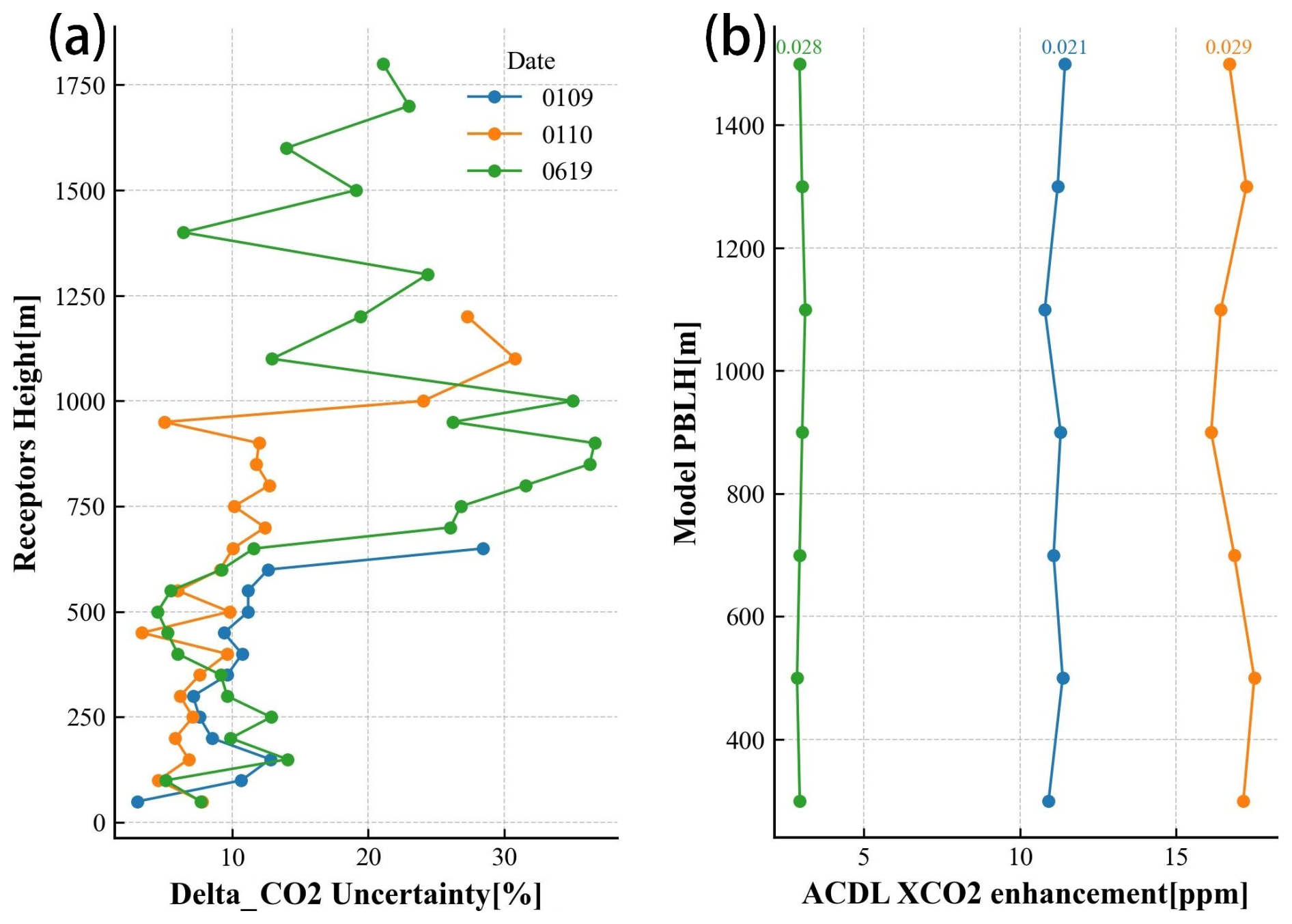
Figure 10 Panels (a) and (b) illustrate the sensitivity of CO₂ and XCO2 enhancements to variations in planetary boundary layer height (PBLH) at different receptor altitudes, quantified by the coefficient of variation (i.e., the standard deviation divided by the mean). Panel (a) presents the simulated results for three satellite overpasses: 23:00 on 9 January 2023 (winter night, blue line), 05:00 on 10 January 2023 (winter day, orange line), and 23:00 on 19 June 2022 (summer night, green line). For each case, receptors were placed at the locations of maximum modeled XCO2 enhancement along the satellite track, with release heights consistent with prior STILT configurations. Panel (b) shows the corresponding XCO2 enhancement simulations for each date, with the coefficient of variation annotated at the top of the panel to indicate the overall sensitivity across varying PBLH scenarios.

Figure 10a illustrates the sensitivity of modeled XCO2 enhancements – calculated following the method in Sect. 2.4.1 – to varying PBLH values at different release heights for three selected receptors. The x-axis, labeled Delta_XCO2 Uncertainty, quantifies this sensitivity as the coefficient of variation (standard deviation divided by the mean) of XCO2 enhancements obtained from simulations with different PBLH values at the same release height. A higher value indicates a stronger response of the modeled enhancement to changes in PBLH. Results in Fig. 10a show that on the nighttime overpass of 9 January 2023 (blue line), the relative variation in modeled XCO2 enhancements remains within ∼ 10 % for release heights below 600 m and does not exceed 13 %, with a minimum of 3.03 % at 50 m. Similarly, for the daytime overpass on 10 January 2023 (orange line), relative variations remain below 13 % up to 950 m, with a minimum of 3.36 % at 450 m. Notably, for this pair of consecutive day–night overpasses, nighttime sensitivity is generally higher than daytime at release heights below 650 m. The nighttime overpass on 19 June 2022 (green line) exhibits a broader vertical range of valid footprints – unlike the 9 January case, where no valid footprints were simulated above 650 m, possibly due to seasonal effects. This case also shows a stronger dependence on PBLH at higher altitudes, particularly between 750–1000 m, with the maximum sensitivity reaching 36.6 % at 900 m. Overall, our findings suggest that within the lower troposphere and across the selected case studies, the influence of PBLH variability on modeled XCO2 enhancements is generally on the order of 10 %, increasing with receptor altitude. As column-averaged observations are less sensitive to the vertical distribution of air parcels (Lauvaux and Davis, 2014), the sensitivity of modeled column XCO2 enhancements to PBLH variations is notably smaller. This is corroborated by Fig. 10b, which shows modeled XCO2 enhancements as a function of PBLH for each overpass, with corresponding coefficients of variation annotated above the lines: 2.1 % (9 January), 2.9 % (10 January), and 2.8 % (19 June) – all lower than the minimum values observed in Fig. 10a.

Given that ACDL is equipped with an aerosol channel, it can provide extinction coefficient profiles and planetary boundary layer height (PBLH) products (Dai et al., 2024). In this study, we utilized ACDL-retrieved PBLH data for forward simulations, which helps to mitigate errors associated with inaccurate PBLH settings. Moreover, since satellite measurements represent column-averaged concentrations, they are inherently less sensitive to variations in PBLH. Therefore, we conclude that PBLH has a negligible impact on the inversion results presented in this study.

5 Conclusions

This study presents the use of DQ-1's XCO₂ observation data to constrain fossil fuel emissions in various urban regions and evaluates its capabilities. By coupling WRF and STILT, a high-resolution forward transport model was developed to simulate and illustrate the structure and details of urban-scale fossil fuel XCO₂ plumes and assess the relationship between simulated and observed XCO₂. Throughout the inversion process, we considered DQ-1's observational errors, transport model errors, and the impact of DQ-1's day-night observation capability on assessing the temporal variation of biosphere fluxes in urban emissions. Employing a Bayesian inversion approach, we optimized CO₂ emissions from fossil fuels in Beijing, Riyadh, and Cairo using DQ-1 data collected from June 2022 to April 2023, focusing on downwind tracks in major urban emission areas where significant XCO₂ enhancements were detected.

Pseudo-data experiments, based on high-resolution forward simulations from real cases, were conducted to evaluate the potential of using multiple DQ-1 tracks while considering measurement and transport model errors. Our results showed that the posterior scaling factors for the three cities ranged from 0.53 to 1.06, 0.75 to 0.86, and 0.98 to 1.21, respectively, with Riyadh exhibiting the highest posterior uncertainty. Notably, some simulations revealed that posterior scaling factor uncertainties are influenced by the relative position of tracks to plumes and positive or negative wind direction biases in the region.

Our assessment of spatial and temporal gradients in biosphere fluxes revealed that, at certain times in Beijing, despite significant ffCO₂ emissions, a notable portion of the local XCO₂ enhancement (20 % and 13 %, respectively) was attributable to local biosphere fluxes. This could lead to an overestimation of total emissions by approximately 33 % ± 20 % and 13 % ± 7 %. By incorporating CASA and ODIAC biosphere flux data and examining day-night crossing tracks on the same day, we found that separately considering day and night biosphere fluxes can improve the accuracy of local XCO₂ enhancement calculations by 30 %–70 % compared to using daily average biosphere fluxes. This indicates that leveraging the short-term, rapid day-night crossing capability of DQ-1, along with more accurate biosphere flux estimation models, has the potential to reduce uncertainties in emission estimates due to biosphere fluxes.

For biosphere flux cities with similar total CO₂ emissions but lower fossil fuel emissions, the contribution of biosphere fluxes is expected to be higher than indicated. Therefore, for cities in mid-latitude and equatorial regions with significant local and regional biosphere fluxes, accurately interpreting XCO₂ detection results is crucial. Future improvements in constraining urban fossil fuel CO₂ emissions using DQ-1 data or other polar orbit measurements should consider the temporal and spatial correlations of previous emission errors, which were not included in this inversion.

For applying these methods to larger-scale flux inversions, advanced satellites with shorter revisit cycles and denser ground-based stations are essential. Additionally, optimizing city emission scaling factors requires more information on prior emission uncertainties to better understand spatial and temporal characteristics of urban-scale emissions. The appropriate number of constraints for urban emissions will depend on the spatial and temporal resolution of target city emissions and the precision required to support policy decisions. Our results demonstrate that DQ-1 or similar missions have significant potential to constrain overall emissions from cities with intensified fossil fuel emissions, and utilizing DQ-1's unique day-night crossing capability, we can establish frameworks for rapid day-night flux inversions at the urban scale. This will further elucidate the spatial and temporal structure of biosphere flux contributions to urban emissions and provide valuable insights for policy-making. We anticipate that DQ-1 data will effectively enhance the accuracy and precision of urban fossil fuel carbon flux estimates, in conjunction with observations from other platforms to support emission reduction strategies.