Operational, diagnostic, and probabilistic evaluation of AQMEII-4 regional-scale ozone dry deposition: time to harmonize our LULC masks

We present the collective evaluation of the regional-scale models that took part in the fourth edition of the Air Quality Model Evaluation International Initiative (AQMEII). The activity consists of the evaluation and intercomparison of regional-scale air quality models run over North American (NA) and European (EU) domains for 2016 (NA) and 2010 (EU). The focus of the paper is ozone dry deposition. Dry deposition is among the most important processes of removal of chemical compounds from the atmosphere and an important contributor to the overall chemical budget of the latter. Furthermore ozone dry deposition is very important as it can be severely detrimental to vegetation physiology. The collective evaluation begins with an operational evaluation, namely a direct comparison of model-simulated predictions with monitoring data aiming at assessing model performance (Dennis et al., 2010). Following the AQMEII protocol and Dennis et al. (2010), we also perform a probabilistic evaluation in the form of ensemble analyses and an introductory diagnostic evaluation. The latter analyzes the role of dry deposition in comparison with dynamic and radiative processes and land use/land cover (LULC) types in determining surface ozone variability. Important differences are found across dry deposition results when the same LULC is considered. Furthermore, we found that models use very different LULC masks, thus introducing an additional level of diversity in the model results. The study stresses that, as for other kinds of prior and problem-defining information (emissions, topography, or land–water masks), the choice of LULC mask should not be at modeler discretion. Furthermore, LULC should be considered as a variable to be evaluated in any future model intercomparison, unless set as common input information. The differences in LULC selection can have a substantial impact on model results, making the task of evaluating dry deposition modules across different regional-scale models very difficult.

1 Introduction

This paper presents the results of the operational and probabilistic evaluation of the regional-scale models taking part in the Air Quality Model Evaluation International Initiative phase 4 (AQMEII-4) activity. As presented in Galmarini et al. (2021), the AQMEII-4 focus is dry deposition process modeling within regional-scale models (AQMEII-4 Activity 1) as well as standalone dry deposition modules (AQMEII-4 Activity 2) as detailed in Clifton et al. (2023).

As traditionally done in past editions of the AQMEII activity (Solazzo et al., 2012a, b; Im et al., 2015), and in agreement with the protocol described by Dennis et al. (2010), prior to any detailed analysis of specific process modeling (diagnostic evaluation), a thorough analysis of the overall performance of the model must be conducted via operational and probabilistic evaluation. The scope of such an approach is to verify the positioning of the models participating in AQMEII with respect to observations or any other model simulating the case study or against a multi-model ensemble (Galmarini et al., 2013). Such an analysis has the scope of assisting the interpretation of any other detailed (diagnostic) result in this paper or other contribution to the special issue and understanding how the different processes contribute to the model spread. Examples of this approach can be found in Solazzo et al. (2012a, b), Vautard et al. (2012), Im et al. (2015, 2018), Giordano et al. (2015), Brunner et al. (2015), and Kioutsioukis et al. (2016). The operational evaluation also provides important context for the interpretation of diagnostic results – for example, the contrast in diagnostic comparisons between models with higher and lower evaluation performance helps to identify specific processes which may contribute to the differences (an example of this approach appears in Makar et al., 2025, this issue, for sulfur and nitrogen dry deposition, as well as Vivanco et al., 2018).

Since the operational and probabilistic analysis is instrumental to the interpretation of ozone dry-deposition-related results (the focus of the fourth edition of AQMEII), we shall concentrate on the variables that are directly or indirectly connected to the description of dry deposition processes within the models, namely atmospheric concentrations, land use/land cover (LULC) masks, and meteorology. A detailed diagnostic analysis of modeled ozone dry deposition can be found in Hogrefe et al. (2025, this issue).

Table 1 Institutions in charge and the models used in AQMEII-4 case studies.

2 Models, domains, and years of consideration

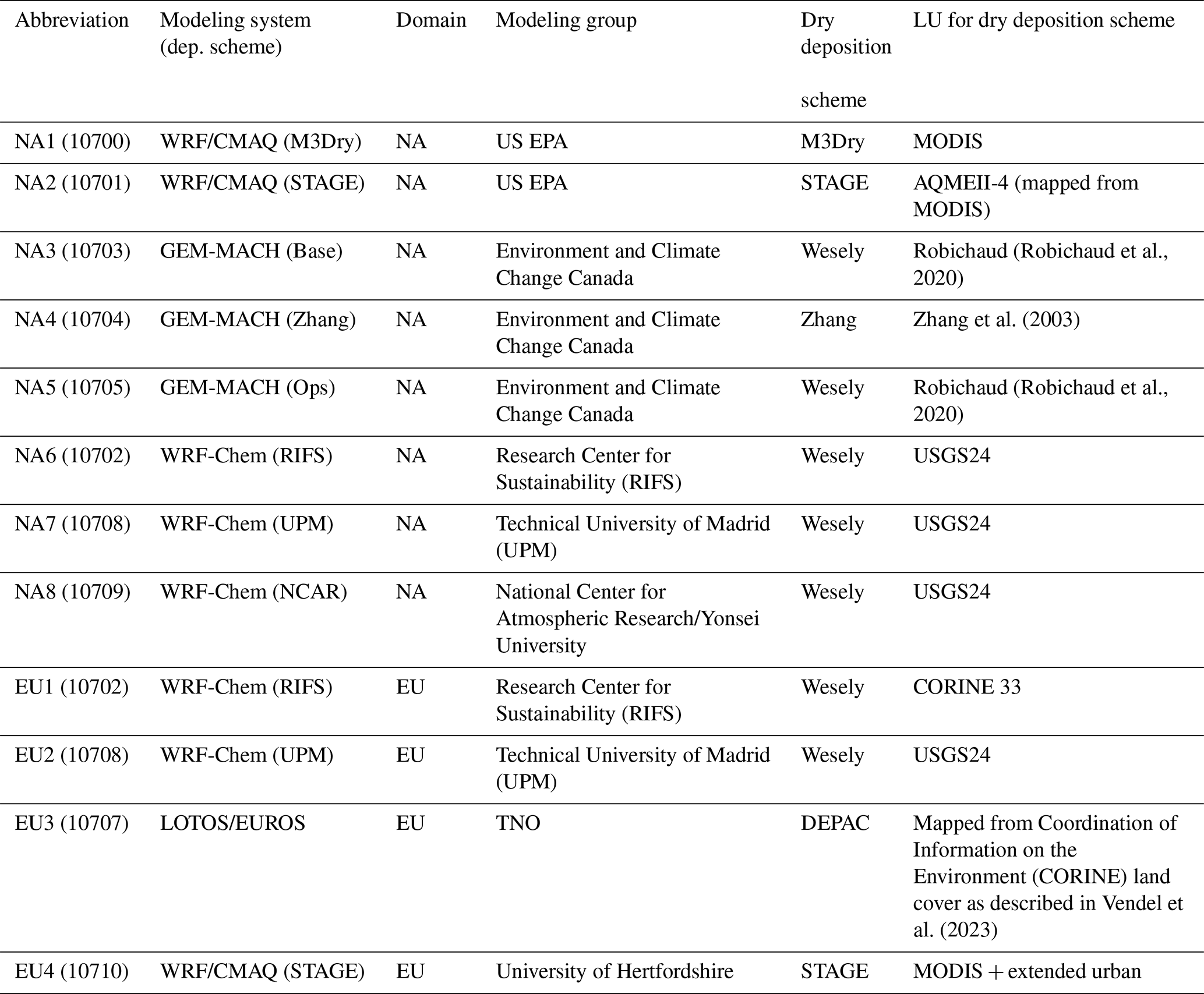
The setup of the AQMEII-4 Activity 1 is detailed in Galmarini et al. (2021). In essence, the activity consists of running regional-scale models on the North American (NA) and European (EU) domains for the years 2010 and 2016 and the years 2009 and 2010, respectively. The motivations behind the selection of these for years are given in Galmarini et al. (2021). The models that took part in AQMEII-4 are listed in Table 1, where details on the institutions in charge and the cases simulated are also provided. These models and in particular their dry deposition schemes are described more in detail in Galmarini et al. (2021, this issue), Makar et al. (2025, this issue) and Hogrefe et al. (2023 and 2025, this issue). Note that simulations took place with harmonized input emissions fields (Galmarini et al., 2021, this issue); all models started with the same anthropogenic, lightning NO_x, and forest fire emissions inventory for North America and Europe, respectively (Galmarini et al., 2021), while biogenic emissions and other natural sources of emissions such those of sea salt particles were carried out as part of internal model processing and should be considered “part of the model” in the analysis that follows.

The analysis described here will only focus on two year-long simulations: 2016 for the NA case and 2010 for the EU case in the interest of synthesis. The following aspects will be considered in detail in this paper:

• Analysis of space- and/or time-averaged ozone concentrations

• Analysis of seasonal, diurnal, and spatial variations of ozone (and to a lesser extent nitric oxide and nitrogen dioxide concentrations in order to assist in the ozone analysis)

• Ensemble analysis of modeled ozone concentrations

• The role of variability in effective fluxes for specific pathways in determining the variability of ozone dry deposition flux over different LULC types

• The role of variability in wind speed, mixed layer height, dry deposition, and radiation in determining the variability of ozone concentrations at the surface

Model values will be evaluated against ozone and precursor concentrations collected by regional operational networks during the year in consideration. More specifically, for North America the monitoring network databases employed included the US Environmental Protection Agency's Air Quality System (AQS; https://aqs.epa.gov/aqsweb/airdata/download_files.html, last access: 30 September 2025), the Canadian National Air Pollution Surveillance (NAPS) program (https://www.canada.ca/en/environment-climate-change/services/air-pollution/monitoring-networks-data/national-air-pollution-program.html, last access: 30 September 2025), and the Canadian National Atmospheric Chemistry database (https://www.canada.ca/en/environment-climate-change/services/air-pollution/monitoring-networks-data/national-atmospheric-chemistry-database.html, last access: 30 September 2025). For the European case the monitoring network databases employed include the European Monitoring and Evaluation Programme (EMEP; https://www.emep.int/, last access: 30 September 2025) and the European Air Quality Database (AIRBASE; https://eeadmz1-cws-wp-air02-dev.azurewebsites.net/download-data/, last access: 30 September 2025). The databases provide measurements in ppb for the NA case and µg m⁻³ for the EU case. We opted for sticking to the original units to avoid a conversion of one into the other to preserve the integrity of datasets and avoid the instruction of uncertainties that would penalize the quality of one or the other.

Given the continental dimension of the two regional domains simulated under AQMEII-4, the latter have been divided into subregional domains for analysis. These group portions of the network that share common features such as atmospheric circulation and possible sources of ozone precursors and also provide continuity with past AQMEII model evaluation phases (Solazzo et al., 2012a, b).

Figure 1 shows the subregions selected within the two modeling domains, the corresponding sampling sites, and the yearly average measured ozone (Fig. 1a and b). As noted by Solazzo et al. (2012a), from the distributions of the pollutants, it is easy to identify the reason for those specific divisions in subdomains. In North America, a longitudinal divide is present between the western (R1), central (R2), and eastern parts of the continent, while the latter also requires a latitudinal division into two smaller subdomains (R3 and R4) due to the different kinds of precursor distributions and consequent ozone formation potentials. In Europe, the spatial distribution of emitters is different from North America and shows greater spatial density. There are areas that require specific attention, being almost decoupled from the rest of the continental airshed. These are typically the Iberian Peninsula and southern Mediterranean basin (R4), the Po Valley (R3), and eastern Europe (R2). These NA and EU analysis subregions were first defined in Solazzo et al. (2012a), though with less detail, and have been used in subsequent AQMEII analyses (e.g., Hogrefe et al., 2018) with different subdivisions but with the same goal of identifying regions with more homogeneous chemical potentials. For the sake of synthesis and in the absence of direct measurement of ozone dry deposition, this paper will concentrate exclusively on the model performance with respect to ozone concentrations with a few references to nitrogen oxides to give a more comprehensive sense of the quality of the performance of the individual models and the ensemble.

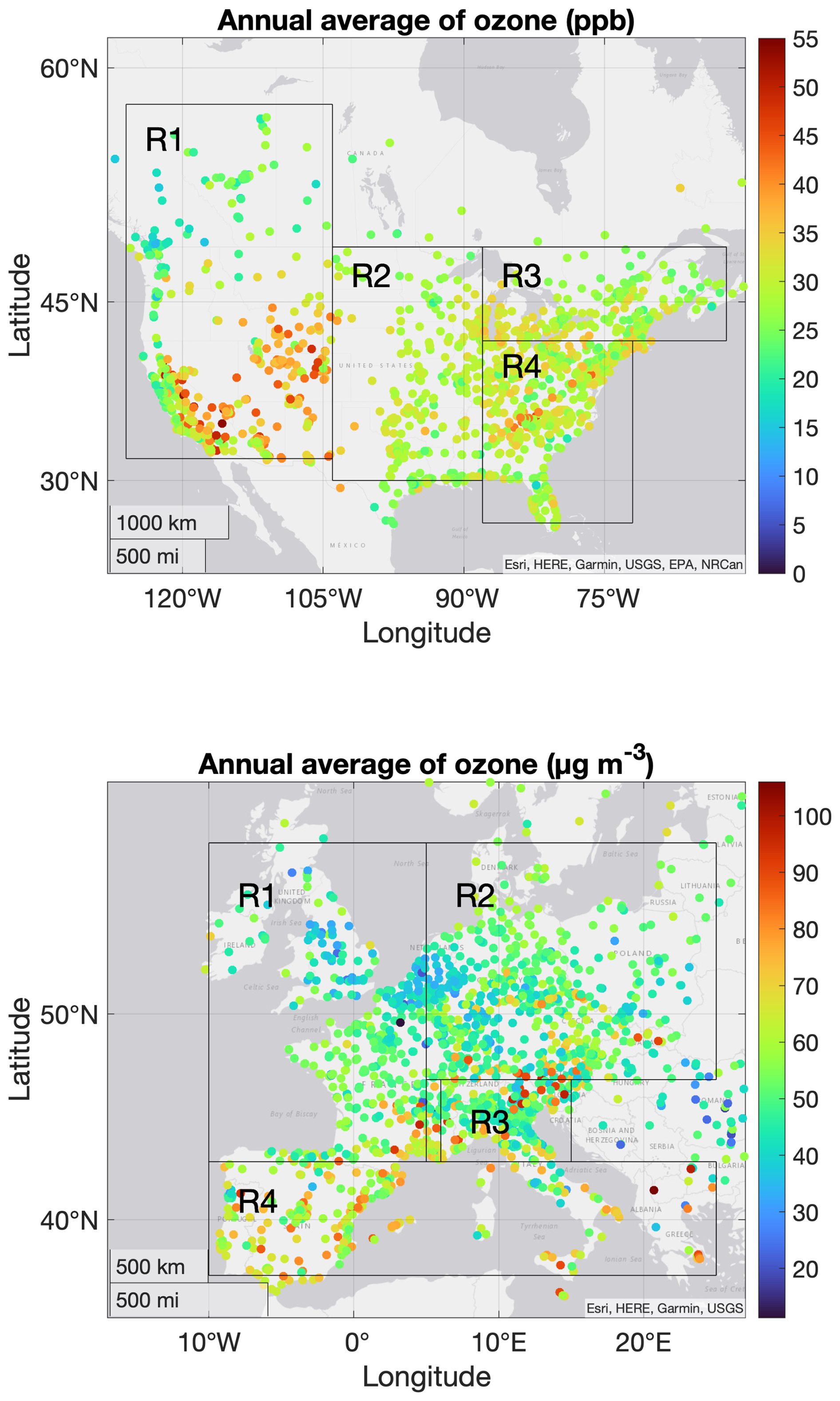
Figure 1 Annual average of ozone at all available monitoring stations in North America for 2016 (a) [ppb] and Europe for 2010 (b) [µg m⁻³]. The rectangular areas represent the four selected subregions (R1, R2, R3, R4).

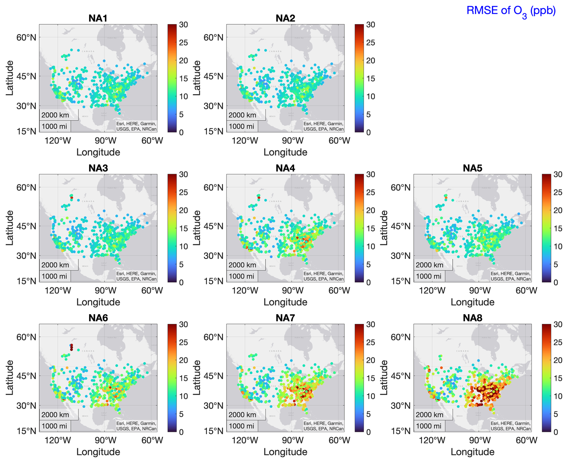
Figure 2 Individual model ozone RMSE calculated over the whole year (2016) over NA. From NA1 through NA8: WRF/CMAQ (M3Dry), WRF/CMAQ (STAGE), GEM-MACH (Base), GEM-MACH (Zhang), GEM-MACH (Ops), WRF-Chem (RIFS), WRF-Chem (UPM), and WRF-Chem (NCAR). Units are in ppb.

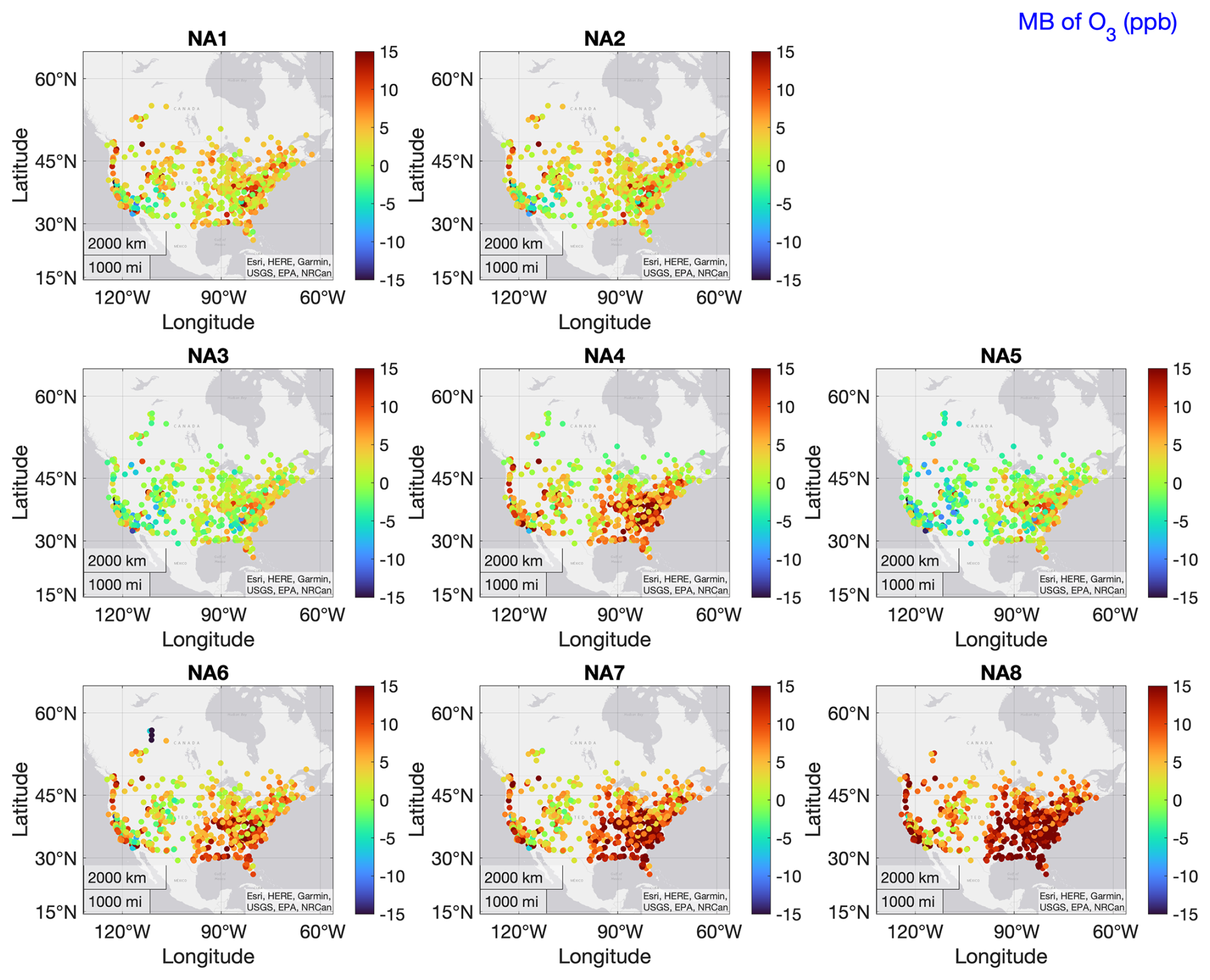
Figure 3 Individual model ozone MB calculated over the whole year (2016) over NA. From NA1 through NA8: WRF/CMAQ (M3Dry), WRF/CMAQ (STAGE), GEM-MACH (Base), GEM-MACH (Zhang), GEM-MACH (Ops), WRF-Chem (RIFS), WRF-Chem (UPM), and WRF-Chem (NCAR). Units are in ppb.

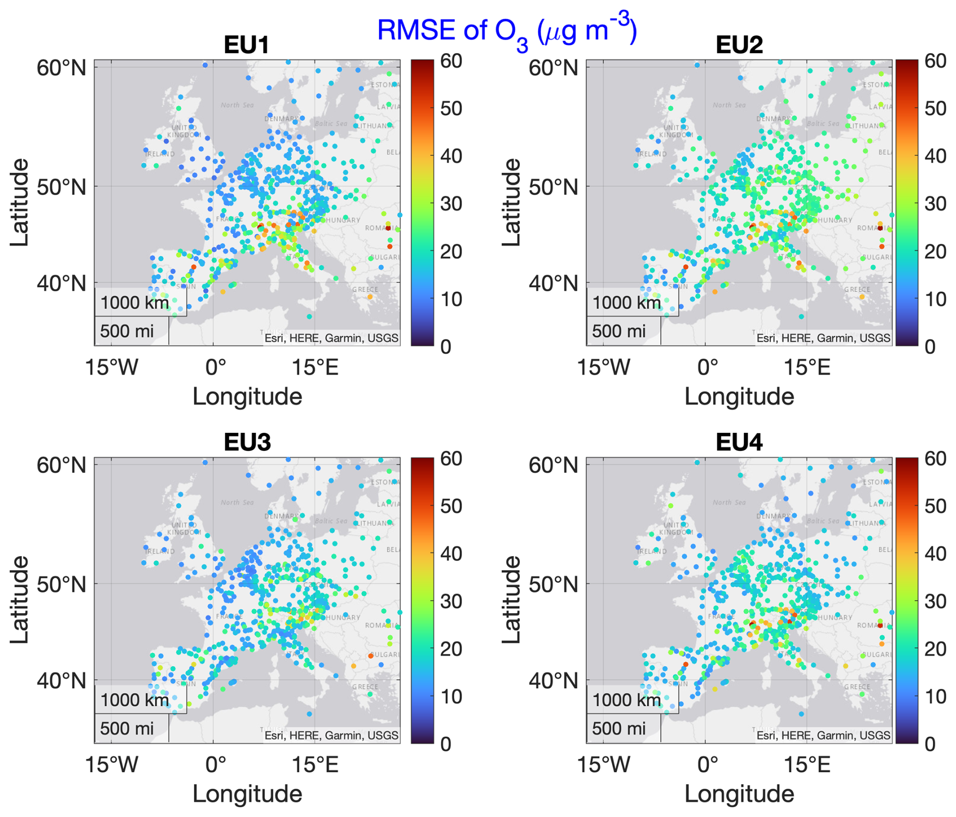
Figure 4 Individual model ozone RMSE calculated over the whole year (2010) over EU. From EU1 through EU4: WRF-Chem (RIFS), WRF-Chem (UPM), LOTOS/EUROS, WRF/CMAQ (STAGE). Units are in µg m⁻³. Color bars are set to twice the range used in Fig. 2 to allow for a visual comparison across continents, accounting for the conversion factor of 1.96 between the different units.

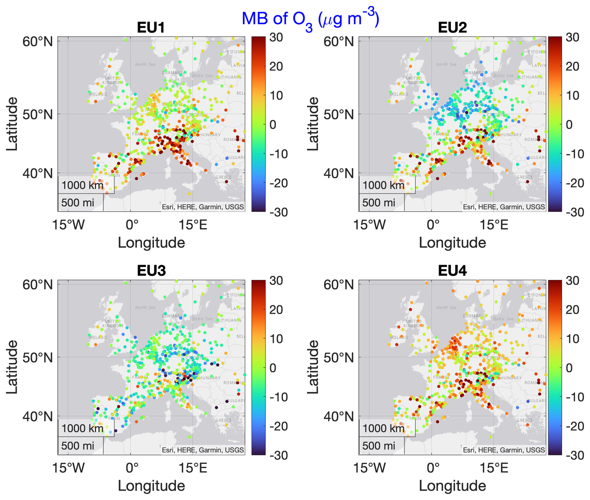
Figure 5 Individual model ozone MB calculated over the whole year (2010) over EU. From EU1 through EU4: WRF-Chem (RIFS), WRF-Chem (UPM), LOTOS/EUROS, WRF/CMAQ (STAGE). Units are in µg m⁻³. Color bars are set to twice the range used in Fig. 2b to allow for a visual comparison across continents, accounting for the conversion factor of 1.96 between the different units.

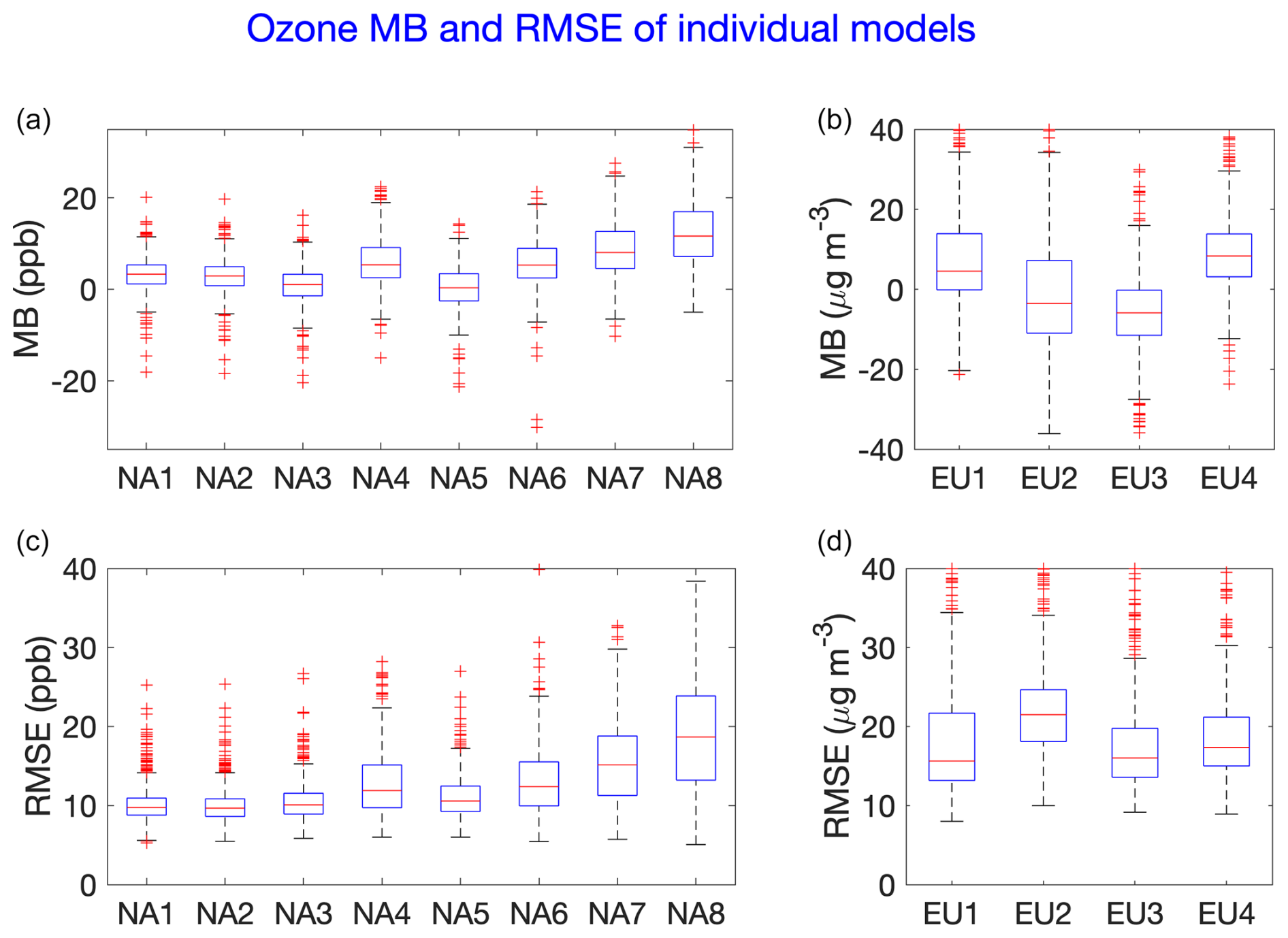
Figure 6 Individual model ozone MB (a, b) and RMSE (c, d) calculated over the whole year over NA (a) and EU (b). NA case units: ppb, EU: µg m⁻³.

3 Operational evaluation

3.1 Ozone and nitrogen oxide surface air concentrations

3.1.1 NA case

The model performances at continental level and for the whole year are presented in Figs. 2–6. For the two continents, the root mean square error (RMSE) and mean bias (MB) are computed from hourly ozone values for the entire year and are shown for each model in Figs. 2 and 3 for North America and Figs. 4 and 5 for Europe. Figure 6 shows the spatially averaged results presented in Figs. 2 through 5 as box plot diagrams. In general, RMSE for the NA case (and in particular, for two models, namely NA7 (WRF-Chem (UPM)) and NA8 (WRF-Chem (NCAR))) appears to be larger than the EU case. Note that, since ozone values are reported in ppb over NA and µg m⁻³ over EU, the range of the color scales over both continents has been set such that the same colors represent the same absolute errors (note the difference in the numerical values for the color bars for these figures) to account for unit differences and allow for a visual comparison between continents. Most differences from the observations are found in the eastern and southeastern parts of the NA domain. As from Figs. 2–5, three groups of behaviors can be distinguished for the NA case. Relative to the rest of the models, NA1, NA2, NA3, and NA5 (WRF/CMAQ (M3Dry), WRF/CMAQ (STAGE), GEM-MACH (Base), GEM-MACH (Ops)) show low RMSE values and comparable behaviors. NA4 (GEM-MACH (Zhang)) and NA6 (WRF-Chem (RIFS)) show slightly higher errors in the middle to east coast part of the domain, whereas NA7 (WRF-Chem (UPM)) and NA8 (WRF-Chem (NCAR)) show markedly higher errors in the middle to eastern part of the domain and along the west coast. Looking at the biases (Fig. 3), the analysis presented above is confirmed with some nuances. In fact, we can see that the grouping can be more refined. A first group is made of the two EPA models NA1 and NA2 (WRF/CMAQ (M3Dry) and WRF/CMAQ (STAGE)) with a widespread overestimation across the continent. NA3 and NA5 (GEM-MACH (Base) and GEM-MACH (Ops)) produce the smallest biases of the group (see also Fig. 3) and with a clearer west–east regional separation compared to NA1 and NA2. Finally, NA4, NA6, NA7, and NA8 (GEM-MACH (Zhang), WRF-Chem (RIFS), WRF-Chem (UPM), WRF-Chem (NCAR)) have larger biases, with NA8 having the largest mean bias (MB) of all (Fig. 4). This analysis helps to distinguish the impacts of different dry deposition modules from the impacts of differences in other aspects of the model on simulated ozone. For example, WRF/CMAQ (M3Dry) and WRF/CMAQ (STAGE) differ only in their dry deposition modules, and the differences between these two simulations are generally smaller than their differences relative to the GEM-MACH and WRF-Chem simulations. On the other hand, the dry deposition scheme has an important effect when we look at NA4 (GEM-MACH (Zhang)) vs. NA3 (GEM-MACH (Base)). These two models share the same regional-scale system but use a different dry deposition scheme. The effect of the dry deposition schemes on the ozone concentration is quite remarkable. Recent work emphasizes a substantial effect of the magnitude of dry deposition velocity on ozone concentration (e.g., Baublitz et al., 2020; Wong et al., 2019; Clifton et al., 2020b). The results are consistent with those in Clifton et al. (2023) where the individual dry deposition module performances were evaluated (see discussion below). Therein larger differences were shown to exist between the Zhang and Base schemes used in GEM-MACH than between the M3Dry and STAGE schemes used in CMAQ. Comparing NA3 (GEM-MACH (Base)) to NA5 (GEM-MACH (Ops)) reveals the impacts of model configuration and science option choices other than dry deposition, since both simulations use the Wesely scheme but differ in a number of other modeling aspects, as described in more detail in Makar et al. (2025). The relatively low MB for models NA3 and NA5 reflects the use of a similar deposition velocity algorithm, while differences between these two models reflect the use of process representations in NA3 which are absent in NA5 (for canopy vertical turbulence different approaches for canopy vertical mixing and photolysis – Makar et al., 2017; feedbacks between chemistry and meteorology – Makar et al., 2015a, b; vehicle-induced turbulence – Makar et al., 2021; and satellite-derived leaf area index – Zhang et al., 2020, while NA5 makes use of a simplified means of adding surface emissions in the model which assumes that fresh emissions are evenly mixed into the first two model layers). The effects of model configuration choices are also evident in the results of the three remaining models (WRF-Chem (RIFS), WRF-Chem (UPM), and WRF-Chem (NCAR)) that share the same dry deposition model and overall model code but utilize different configuration options. These simulations show a consistent overestimation that cannot be attributed clearly to one factor (see also Fig. 3). The three implementations are also with respect to three different WRF-Chem version numbers (3.9.1, 4.0.3, and 4.1.2, respectively); versions 3.9.1 and 4.0.3 use the Grell and Devenyi (2002) cumulus parameterization, and version 4.1.2 uses the Grell and Freitas (2014) parameterization. Furthermore, both WRF-Chem (RIFS) and WRF-Chem (UCAR) employ the same gas-phase mechanism (Emmons et al., 2010), while that of WRF-Chem (UPM) differs from the other two models. The relatively minor differences between WRF-Chem (UPM) and WRF-Chem (UCAR) shown in Fig. 6a may thus reflect differences in the gas-phase chemistry, with the former's mechanism resulting in slightly lower positive bias levels. Knote et al. (2015) conducted a comparison of the two gas-phase mechanisms (CBMZ and MOZART4) within the same modeling framework and showed that the two mechanisms have biases opposing in both magnitude and sign over North America. The larger differences (same figure) with the RIFS implementation reflect differing cloud amounts and hence differing photolysis rates within the two implementations. The large overestimation of ozone by the WRF-Chem (UCAR) configuration may thus be linked to the underestimated precipitation in this model reported elsewhere (e.g., Makar et al., 2025), which also implies smaller cloud amounts and stronger solar radiation.

3.1.2 EU case

In Figs. 4 and 5, RMSE and MB in Europe are presented, respectively. The errors have more a hot-spot character that is mainly evident in the southern part of the domain and therein at well-recognized critical regions like the Po Valley in the north of Italy, Greece, and the Iberian Peninsula. This result is confirmed in the MB plots that also show EU3 (LOTOS/EUROS) as the best-performing model of the four though in many cases underestimating ozone concentration levels. EU2 shows worse RMSE scores than the other three models, in particular over Germany, Poland, and Hungary, and scores the highest median RMSE value (Fig. 6b). As for the rest of the domain, smaller RMSE values can be noticed throughout the region for all models. EU1 (WRF/Chem (RIFS)) and EU4 (WRF/CMAQ (STAGE)) show comparatively larger errors, especially in the southern and northern parts of the domain, respectively. This behavior of EU1, EU2, and EU4 may be associated with the prediction of NO₂ and NO concentration (see later discussion).

In this case, a model implementation/user effect can be an element of consideration since the EU4 is the same model that is used by the EPA in the NA case (NA2), but in this instance run by the University of Hertfordshire. In the implementation of EU4, the primary differences lie in the meteorological model and the MEGAN biogenic emissions input. These variations in meteorological drivers and biogenic emissions can introduce differences, potentially contributing to the observed model biases when compared to other implementations of the same model. However, it should also be noted that the CMAQ simulations in North American (models NA1, NA2, Fig. 3) also show positive biases, particularly along the US eastern seaboard. Some of these biases may be attributable to the need for physical process representation for forest canopy shading and turbulence (see Makar et al., 2017, which intercompares multiple models) and has been found more recently to improve the performance of the CMAQ model (Campbell et al., 2022; Wang et al., 2025). Many of the regions with the highest ozone biases in models EU1, EU2, and EU4 correspond to areas with high forest canopy and leaf area index values, as does the eastern seaboard of the USA and Canada, and the negative biases in EU1 and EU4 for NO and NO₂ are consistent with the absence of the more realistic reduction in thermal diffusivity coefficients and photolysis rates expected under forest canopies (Makar et al., 2017); the performance of these models may be improved through the inclusion of forest canopy processes.

From the analysis of NO, NO₂, and O₃ normalized root mean square error vs. normalized mean bias in the soccer plots of Fig. S1 in the Supplement for the two continents, we note that the two precursors to ozone show an error smaller than 15 % for all models except two. For the NA case, the ozone soccer plots confirm the grouping of the results qualitatively derived from the regional analysis of Fig. 2. Figure 6 shows that GEM-MACH models NA3 and NA5 have ozone bias values closest to zero, followed by CMAQ (NA1 and NA2), while CMAQ has the lowest RMSE values, closely followed by the GEM-MACH NA3 and NA5 implementations. Four models show small error (< 15 %), two with medium (> 15 % and < 20 %) and two with high (> 20 %). The ozone goal plots for the EU (Fig. S1) show a statistical tendency to produce smaller errors than the NA case and in particular more coherence between the errors for ozone and its precursors.

The Taylor diagram depicted in Fig. S2 also evaluates the correlation between simulated and observed ozone values. The results show a higher correlation of model predictions with observations in the EU case, while the other statistical parameters in the diagram confirm what has been presented in the other plots. The multi-model ensemble (MME) is also presented for the two cases, showing in both instances an improved performance with respect to the individual model simulations.

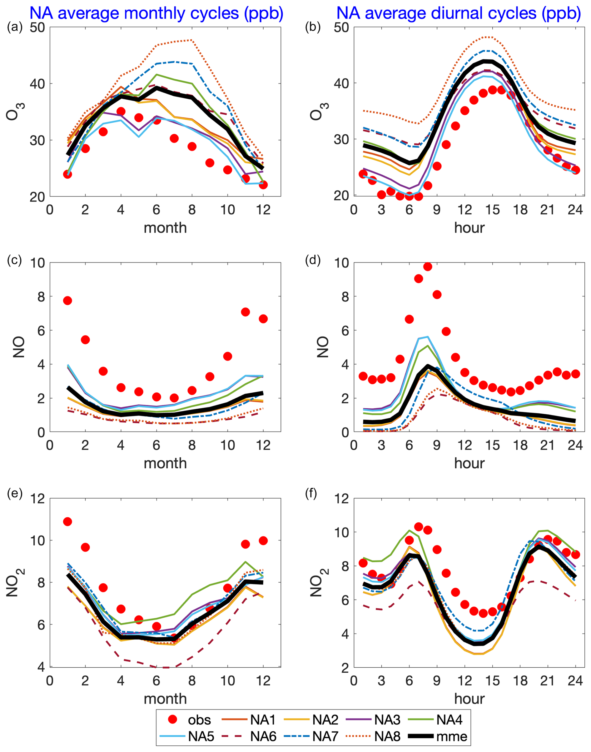
Figure 7 Average monthly (a, c, and e) and diurnal (b, d, and f) cycles of ozone, NO, and NO₂ [ppb] for the 2016 NA case study. Thin colored lines (solid, dashed, dotted): models; red dots: observations; black line: multi-model mean.

3.1.3 Diurnal and seasonal variability

Figure 7 shows a comparison of observed and modeled seasonal and diurnal cycles for North America for ozone, NO, and NO₂. These cycles were constructed by averaging the underlying raw hourly data available for the entire year over a given month of year or hour of day, respectively. At the monthly level, the figure clearly shows that for ozone in NA, almost all models overestimate the concentration during summer. The multi-model mean fails to reproduce the ozone maximum in April by overshooting by approximately 3 ppb and presenting a maximum in June. This result is driven by four out of eight models (NA4 (GEM-MACH (Zhang)), NA6 (WRF-Chem (RIFS)), NA7 (WRF-Chem (UPM)), and NA8(WRF-Chem (NCAR))). Although slightly overestimating the concentration, two models (NA3 (GEM-MACH (Base)) and NA5 (GEM-MACH (Ops))) manage to reproduce very accurately the seasonal evolution. NA1 and NA2 (WRF/CMAQ (M3Dry) and WRF/CMAQ (STAGE)) capture the trend and seasonality and just slightly overestimate the ozone peak value.

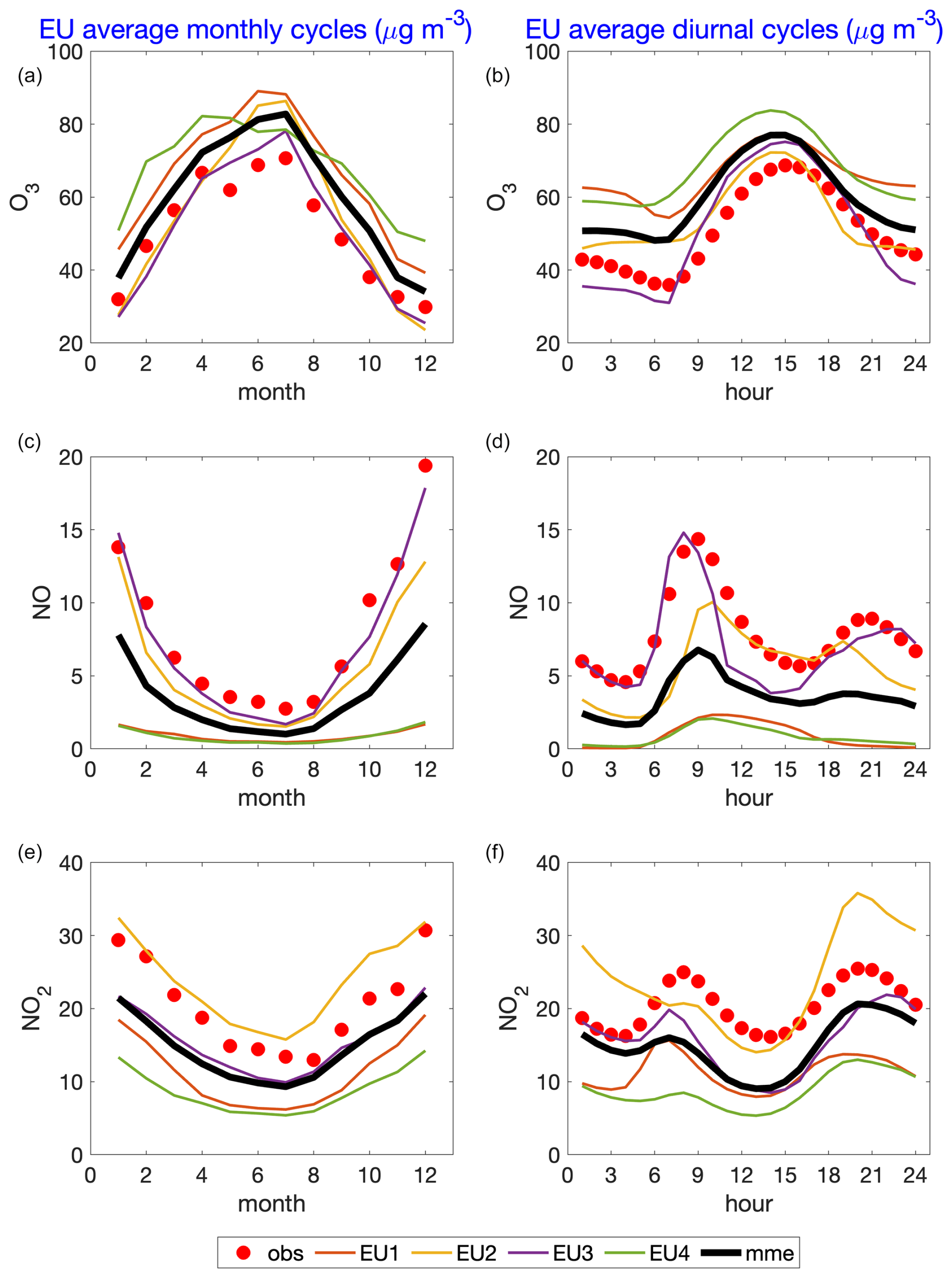
Figure 8 Average monthly (a, c, and e) and diurnal (b, d, and f) cycles of ozone, NO, and NO₂ [µg m⁻³] for the 2010 EU case study. Thin colored lines: models; red dots: observations; black line: multi-model mean.

The tendency for overestimating ozone concentration and underestimating NO is also clear from Fig. 7 (for NA) and Fig. 8 (for EU). Figure 7's diurnal variation panels (Fig. 7b, d, and f) in particular show that the models NA3 and NA5 have the closest values to observations for O₃, NO, and NO₂, though all models underestimate the NO_x totals. This is especially evident for NO and NO₂ in the midday hours (10:00 to 18:00 LT), when the simulated NO and NO₂ values are the closest in the ensemble to the observations. The monthly variation panels (Fig. 7a, c, and e) show that the relative impact of the NO_x underestimates is smaller in the summer than in the winter, and models NA3 and NA5 have the closest NO values to observations and slightly overestimate NO₂ in the summer. Model NA3 includes a forest canopy parameterization (Makar et al., 2017), which takes into account reduced vertical coefficients of thermal diffusivity and photolysis levels below the forest canopy – these in turn reduce turbulent mixing (resulting in higher NO_x concentrations from surface sources) and also shift the chemical regime from ozone production to ozone destruction by NO_x titration below the forest canopy. Model NA3 also includes the effects of vehicle-induced turbulence on NO_x emissions from vehicles (Makar et al., 2021), an effect which results in more efficient dispersion of these emissions out of the surface layer. Model NA5 assumes the area emissions of NO_x are evenly and instantaneously distributed over the first two vertical levels of the model rather than incorporating these emissions as a flux boundary condition on the diffusion equation. As noted above, Models NA3 and NA5 include process representation which can enhance the vertical transport of freshly emitted NO_x out of the lowest model layer; at least some of superior performance may be related to this faster dispersion. The ozone dry deposition velocity used in NA3 and NA5 versus that of NA4 is also a driver for the differences between these models, as noted in Clifton et al. (2023), who noted that NA3 and NA5 shared a scheme which significantly overestimated ozone dry deposition velocities relative to observations in the summer while providing reasonable estimates during the winter, while the Zhang scheme, used in NA4, showed little seasonal variation (tending to be flat over time, with overestimates during winter and underestimates during summer). It is of note that the models that reproduce the seasonal evolution of ozone most accurately during summer when the rest of the models struggle have the dry deposition schemes with the largest positive biases in summertime ozone dry deposition velocity and the greatest seasonal amplitude (Clifton et al., 2023). This implies (1) that the factors affecting the ozone concentrations have a strong seasonal dependence (models NA4 versus NA3 and NA5) (2) and that while one means of helping achieve that seasonal dependence is through an overestimation of the ozone dry deposition velocity relative to observations (models NA3 and NA5), (3) other seasonally dependent process improvements than dry deposition velocity are required to better simulate ozone (given that the other models considered here which incorporate more accurate ozone dry deposition schemes, relative to the observations in Clifton et al., 2023, also have high positive biases in parts of NA and EU; Figs. 3 and 5). As noted above, process representation of forest canopy shading and turbulence is one such possible means of model performance improvement¹. The other consideration worth examining is the interdependence between model cloud cover and surface photolysis rates, given the variation between NA WRF-Chem models NA6, NA7, and NA8, where the largest differences in ozone positive bias correspond to the use of differing cloud parameterizations.

For NO and NO₂, the models show seasonal cycles which differ between the models (Figs. 7a, c, e and 8a, c, e) versus the observations and between the NA and EU observations. Observed NA ozone peaks in April (month 4, Fig. 7 upper left panel), while observed EU ozone peak in July (month 7, Fig. 8 upper left panel). As noted above, models NA1, NA2, NA3, and NA5 all capture the NA O₃ seasonality (CMAQ and Base and Ops GEM-MACH configurations), while the WRF-Chem models predict a late summer peak, similar to observations in EU. All models tend to overestimate compared to observed ozone concentrations (exceptions: NA3 and NA5 in April and May, Fig. 7, EU2 and EU3 from November to April). All models underestimate wintertime NO_x (though NA models NA1, NA2, NA3, NA5, and NA7 have close NO₂ performance to observations from July through October, Fig. 7), and EU3 NO values closely match observations, while EU2 NO₂ is biased high relative to observations. All NA models have significant (factor of 2 or more) negative biases in NO and the largest seasonal NO₂ negative biases in winter. As a consequence, all NA models strongly underestimate the amplitude of the observed seasonal cycle. Potential factors which might drive an underestimate of wintertime NO_x include underestimates in the emissions of NO_x from combustion sources such as wintertime home heating from fossil or wood fuels (Denier van der Gon, 2015), underestimates of atmospheric stability (i.e., if the simulated atmosphere is more unstable than the actual atmosphere, NO_x emissions may build up to higher concentrations in the model than is observed), and the potential for HONO cycling in the presence of snow on the surface, leading to longer lifetimes of NO_x (Michaud et al., 2015). Figure 8 also shows, not unexpectedly, that the models with the smallest NO and NO₂ biases (EU2 (WRF-Chem (UPM)) and EU3 (LOTOS/EUROS)) do quite well for O₃, NO, and NO₂, and the EU NO and NO₂ biases for these models are in general much smaller than the NA model biases. At the diurnal level (Figs. 7 and 8 right panels) the results are consistent with what is found at the seasonal level in terms of overestimations or underestimations. At the diurnal level, EU2 outperforms the others, showing a good capacity to catch the average time evolution of the three pollutants.

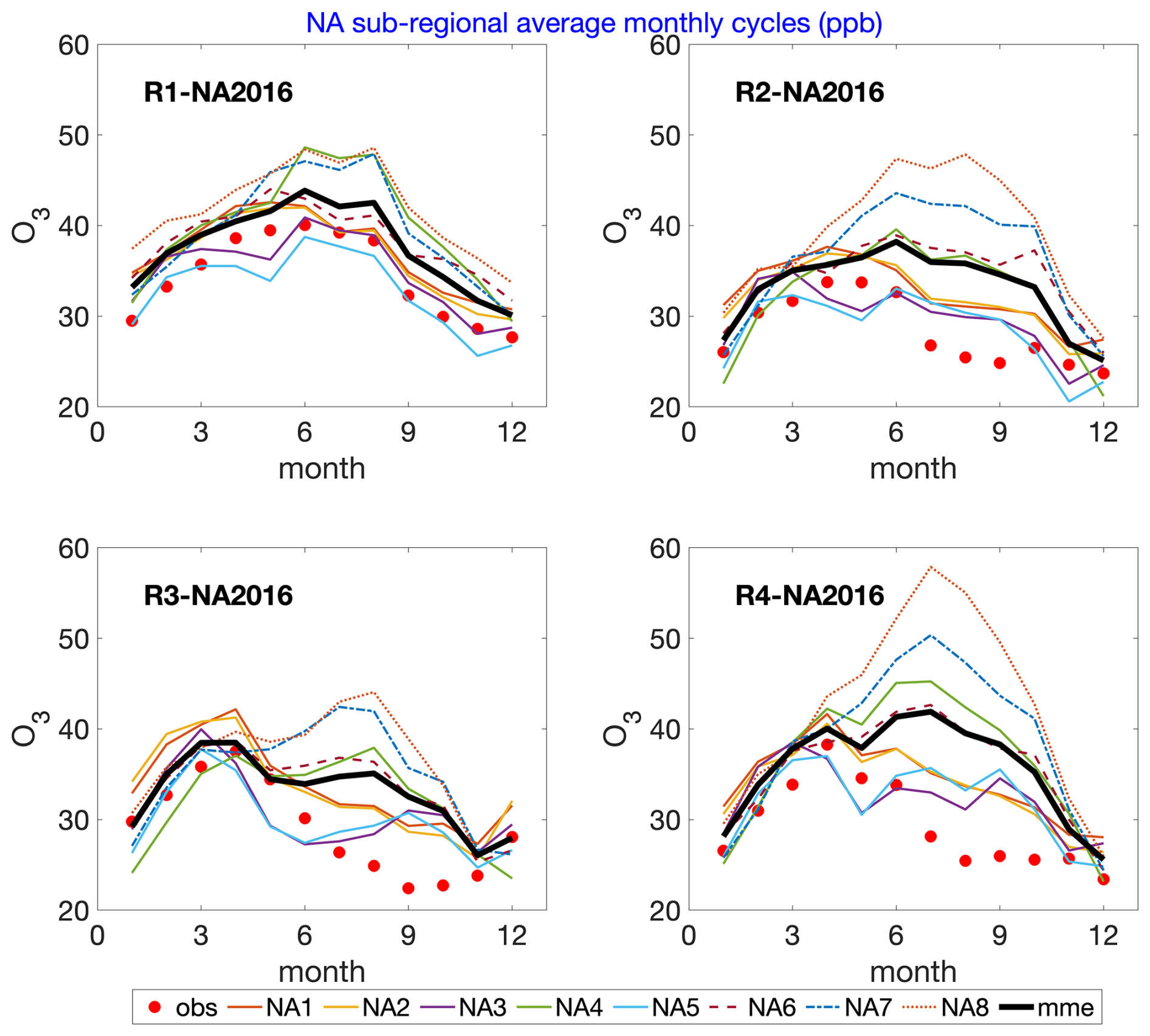
Figure 9 Monthly average cycles of O₃ concentrations in [ppb] as calculated in subregions R1–R4 over the NA domain. Thin colored lines (solid, dashed, dotted): models; red dots: observations; black line: multi-model mean.

The monthly averaged ozone, NO, and NO₂ concentration breakdowns at the subregional level are presented in Figs. S3 and S4 for NA and EU, respectively. From Fig. S3 one can conclude that the major contribution to the domain-wide estimation presented earlier is essentially coming from regions R2, R3, and R4 (i.e., the eastern part of the domain), whereas all model results in R1 are rather similar and in agreement with the measurements throughout the year, with some models overestimating cold seasons but to a lesser extent than in the other regions. The summertime ozone overestimation over the eastern US for NA1 and NA2 (WRF/CMAQ (M3Dry) and WRF/CMAQ (STAGE)) is consistent with the findings of Appel et al. (2021). It is also worth noting that all of the NA models (Fig. 9) overestimate O₃ in the period from July through September in regions R2, R3, and R4, an observed effect largely absent in the EU models (Fig. 10). We also note that the time series of observed O₃ for North America shows April peaks for regions R2, R3, and R4, while R1 peaks in June. One possible cause for the observed early spring peak in the latter regions is the transport of upper-tropospheric O₃ downwind of the Western Cordillera, a process which is known to be at its maximum in the springtime (Pendlebury et al., 2018). From Fig. S4, referring to the EU case, we see that EU1 and EU4 underestimated NO and NO₂, whereas EU2 largely overestimates for all European subregions. Such model performances can explain the ozone biases as they affect ozone titration at night. This effect is apparently exacerbated in the Po Valley area, which is known for high NO_x emission levels. The observational sites in the Scandinavian Peninsula are mainly from the EMEP network, which is representative of the remote background, whereas the AIRBASE network rural background sites are more prone to local sources of pollution.

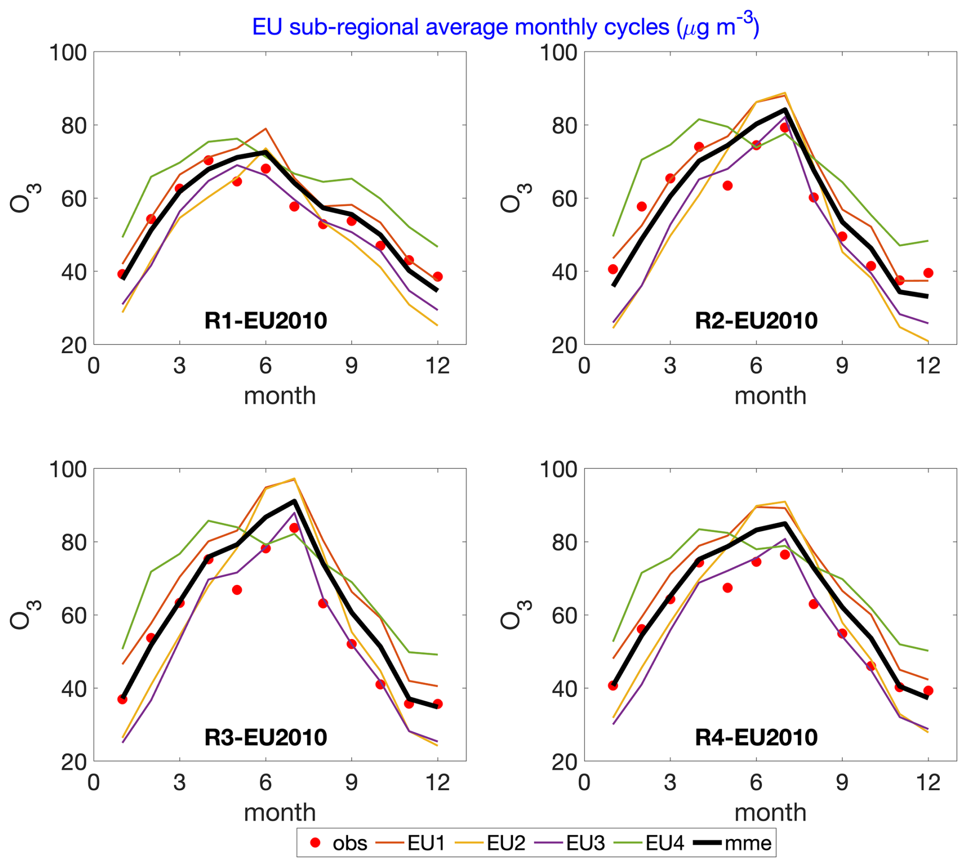
Figure 10 Monthly average cycles of O₃ concentrations in [µg m⁻³] as calculated in subregions R1–R4 over the EU domains. Thin colored lines: models; red dots: observations; black line: multi-model median.

These regional differences will be instrumental to the analysis of dry deposition processes. The same behavior observed in subregions is found at both the seasonal and hourly level. From Fig. 10 we can see the situation in Europe, which lacks the large positive biases in the NA simulations.

3.1.4 Summary of the analysis

Overall conclusions from the comparisons with observations for NO, NO₂ and O₃ are the following:

• the models which most closely match NO and NO₂ (EU2, EU3) also have the best performance for O₃

• models with negative biases for NO and NO₂ also have positive biases for O₃, and the magnitude of the NO_x negative biases is inversely proportional to the magnitude of the O₃ positive biases for all models

• the relative magnitude of the “freshly emitted” component of NO_x (i.e., NO) tends to be underestimated, with the exception of model EU3 (LOTOS/EUROS)

These results all point towards excessive vertical mixing of fresh NO emissions up from the lowest model layer as a root cause of the model biases in the other models. The reasons for this conclusion are the following:

1. the relative fraction of NO_x that is NO will be highest in air dominated by fresh emissions;

2. the relationship between positive ozone biases and negative NO biases indicates that the ozone biases are due to insufficient NO titration;

3. the effect is exacerbated in winter in all NA models and some EU models – a time when the atmosphere tends to be more stable, and photolysis rates in the Northern Hemisphere are low, both conditions which favor NO_x titration.

A secondary cause may be missing NO emissions in the wintertime, though this seems less likely due to the relatively high confidence in mobile emissions and stack emissions, which dominate the NO_x emissions totals, and the relatively good performance of EU3 relative to the other EU models when making use of the same emissions inventory.

3.2 Ozone dry deposition fluxes

We start our examination of O₃ dry deposition fluxes with the direct comparison of the effective and total fluxes calculated by the models. Effective flux is a convenient way of examining the contribution of the resistances of various pathways towards bulk dry deposition, taking into account that variability is not only due to these resistances but also surface ozone concentrations (Galmarini et al., 2021). The definition of effective fluxes is analogous to the definition of effective conductances (Paulot et al., 2018; Clifton et al., 2020b). Specifically, by definition, the sum of the effective fluxes equals the total ozone dry deposition flux, and this equality is used in the subsequent analysis. Within AQMEII-4, the relevant effective conductances were defined a priori and every participating modeling group was requested to determine the combination of all relevant resistances accounted for in their systems, necessary to produce the effective conductances requested. The definitions of the effective conductances, the dry deposition modeling approaches, and the detailed formulation of effective fluxes for each model are presented in Galmarini et al. (2021, this issue). Because effective conductances and ozone concentrations can covary on daily timescales, it was important to archive high-frequency effective fluxes; for this same reason, conclusions about drivers of variations in effective fluxes may be distinct from those regarding effective conductances. The analysis of effective and total fluxes is performed only for the grid cells in which all models share the same LULC (for details on the common LULC classifications see Galmarini et al., 2021, this issue). By restricting the analysis to locations sharing the same characteristics of land use across models, we reduce the impact of LULC variability on the resulting analysis, thus allowing us to compare only the response of models to the different dry deposition schemes employed for a given LULC. We present model results at grid cells that are covered by at least 85 % evergreen needleleaf forest (NA: 1544 cells, EU: 2531 cells) and planted-cultivated (NA: 6130 cells, EU: 6108 cells). In addition, we also define an “ozone receptor” case that corresponds to the grid cells where ozone is monitored at the surface for the two continents (NA 1551 cells, EU 1656) independently from the underlying LULC type, which can therefore be different from model to model. In the Supplement the deciduous broadleaf forest (581 cells) and mixed forest (705 cells) are also presented for the NA case only for the sake of synthesis.

An important finding is obtained by simply imposing the data selection criterion described above. As can be noted, for the same continent the models share relatively few grid cells with the same dominant LULC. This is a clear indication of the fact that individual LULC masks, employed in the models, were obtained from substantially different sources (Table 1). Such results raise a significant issue: is it acceptable that the characterization of the land surface differs so much? In principle LULC masks adopted by the AQMEII-4 models should be very comparable, especially when sources of this information with a high degree of spatial resolution are now available. More discussion may be found in Sect. 5 and in our companion paper (Hogrefe et al., 2025, this issue).

Figures S5 and S6 show seasonal cycles of the total ozone dry deposition flux and its decomposition into the three different effective fluxes. The pathways represented by these effective fluxes are (1) lower canopy and soil conductances combined in one factor (LCAN + SOIL) since some models did not distinguish these two terms, (2) cuticular conductance (CUT), and (3) stomatal conductance (ST).

The following features can be appreciated across the model results:

• The magnitude peak of the ozone flux varies considerably from model to model in some cases (NA8), being almost twice that of others (NA4) for the monthly average.

• Typically, the flux is highest during summer and lowest during winter. In some cases, some fluxes show nearly constant values throughout the summer season (NA2, NA3, NA5, and NA7). In others, there is a stronger midsummer peak (NA1, NA4, NA6) in July or August. NA8 shows a double-peak shape. Given that the dry deposition scheme is the same in NA8 as NA7 and NA6, this suggests that this double peak is either meteorologically driven or ozone-driven.

• In the EU case more homogeneity appears between EU1 and EU2 behaviors, while EU4 shows a slightly different performance for this macrolevel analysis at least.

The breakdown of the contributions of the specific pathways to the total ozone flux does not appear to identify any common behavior either across models or within the same LULC type or across time. It is particularly notable that the relative contributions of the different pathways vary between models (e.g., compare the relative magnitude of stomatal flux in NA1 and NA2, Fig. S5a). Some models employing the same dry deposition algorithm nevertheless have different contributions associated with the different pathways (see NA3 versus NA5, which have the same dry deposition algorithm, yet the soil term dominates in NA3 and the cuticle term dominates in NA5). The difference in soil versus cuticle terms dominating in NA3 and NA5 likely reflects differences in meteorology between these two model implementations; as noted above, NA3 includes feedbacks between meteorology and chemistry, in turn resulting in differences in the meteorological terms controlling these two deposition pathways.

We note that an exception to the explanation presented above is for the “planted-cultivated” LULC, where ST and LCAN + SOIL tend to dominate the flux. There is also a clear summer maximum in ST across models (Fig. S5e), but the exact seasonality of ST differs significantly between models. LCAN + SOIL tends to have a bimodal seasonality for this LULC type – with minima during winter and during times of maximum ST. CUT tends to be low – with NA1 and NA2 suggesting slightly higher values – with weak but noticeable seasonality with a broad growing season peak. To a certain extent, this pattern in seasonal variation in the different pathways and their contribution to the total flux also shows up for deciduous forests (Fig. S5c), but less so for CMAQ than for the other models. In general, stomatal flux tends to drive seasonality in the ozone flux, as Clifton et al. (2023) found for ozone dry deposition velocity at the individual flux sites, but sometimes there is a seasonal contribution in non-stomatal flux. The models also all differ in the relative contributions of LCAN + SOIL, CUT, and ST, as also found by Clifton et al. (2023). For example, cuticular flux is very low in some models (e.g., WRF-Chem) but a dominant contributor (about $\mathrm{1}/\mathrm{3}$ except over crops) in NA1 and NA2. Perhaps the primary conclusion is that model behavior can be grouped around the model type. In fact, clear similarities can be found among NA3 and NA5 (GEM-MACH (Base) and GEM-MACH (Ops) for several land use types), as well as NA6, NA7, and NA8 (WRF-Chem (RIFS), (UPM), and (NCAR), respectively). In the EU case, EU1 and EU2 (both WRF-CHEM) have comparable yearly characteristics, while EU4 (WRF/CMAQ (STAGE), used by the University of Hertfordshire) shares a similar breakdown with NA2 (WRF/CMAQ (STAGE), run by the USA-EPA).

Although relevant for operational evaluation, the analysis in Figs. S5 and S6 does not easily reveal the significance of dry deposition processes and pathways in determining ozone variability across models. Toward this end, hierarchical and variation partitions are considered in Sect. 5.

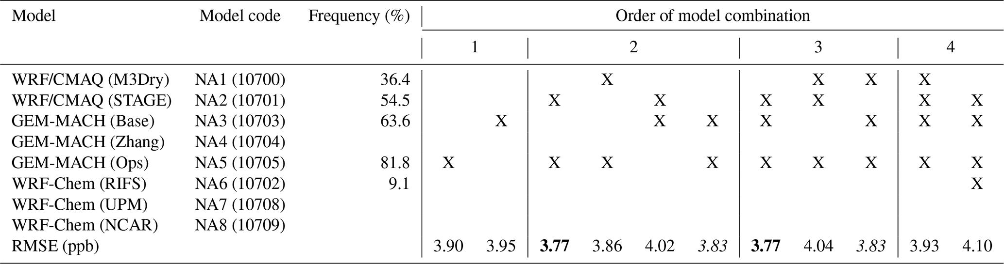
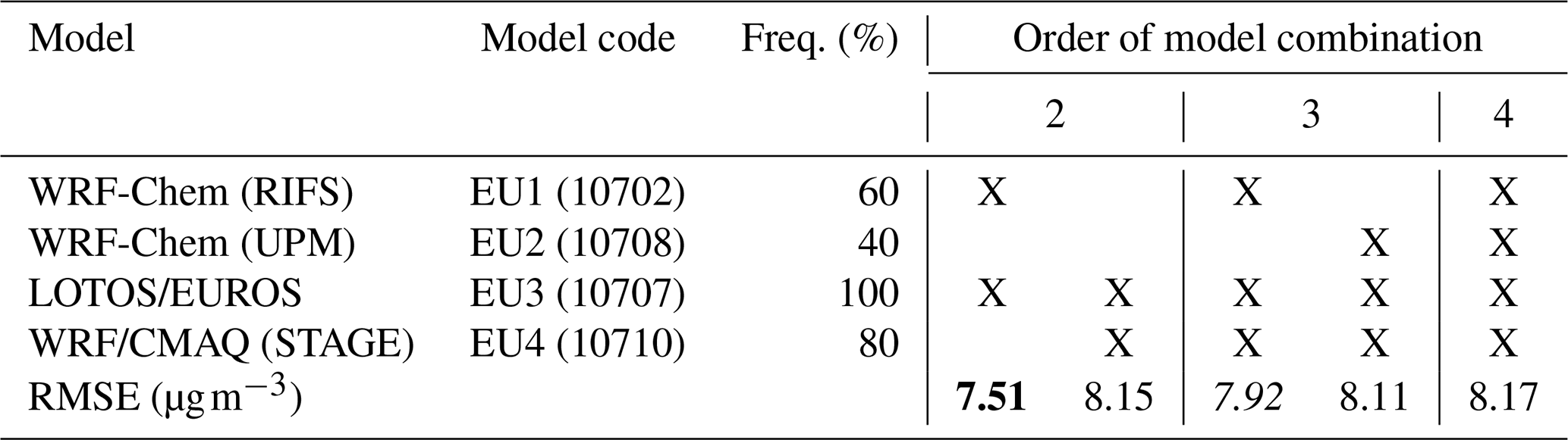
Table 2 NA case. For all available combinations of models analyzed, the table presents those that produce the minimum errors (blue columns) as well as all other combinations that fall within 10 % of that minimum error (yellow and orange columns). The minimum RMSE of 3.77 ppb is achieved by the second-order (, all combinations of two models out of eight) combination of WRF/CMAQ (STAGE) and GEM-MACH (Ops) as well as the third-order (, all combinations of three models out of eight) combination of WRF/CMAQ (STAGE), GEM-MACH (Base), and GEM-MACH (Ops). The combinations with the lowest and second-lowest RMSE are shown as RMSE values in bold and italics, respectively. The frequency column shows the number of times each model was part of an ensemble weighted by the number of ensembles considered.

4 Probabilistic evaluation

The ensemble analysis described in this section aims to identify the models that contribute to an improved ensemble result and the best combination of models that improves the ensemble skill. Such analysis is part of the probabilistic evaluation described in Dennis et al. (2010) and constitutes one of the four pillars of evaluation defined therein and adopted in the overall AQMEII activity. In past phases of AQMEII, ensemble analysis was also presented as an integral part of the model evaluation (Solazzo et al., 2012a, b, 2013a, b, 2017b; Galmarini et al., 2013; Kioutsioukis and Galmarini, 2014; Im et al., 2015; Kioutsioukis et al., 2016; Galmarini et al., 2018). The ensemble mean of the model results has already been presented in the operational analysis. However, identifying which and how many models contribute to improved ensemble results is another question to be addressed in this context. The analysis uses ozone mean concentration measured at the monitoring sites as a reference and techniques based on model combination to determine the optimal results as described in earlier studies (Solazzo et al., 2012a, b, 2013a, b; Galmarini et al., 2013, 2018; Kioutsioukis and Galmarini, 2014; Kioutsioukis et al., 2016).

The skill of an ensemble increases if we combine accurate and diverse models (Kioutsioukis and Galmarini, 2014). As shown by Solazzo et al. (2012a) the skill normally reaches a maximum for an ensemble composed of fewer than half of the available models and then deteriorates when more models are added until reaching an asymptotic value. Given m available models, several combinations of model results in groups of n≤m can be produced. In this analysis, we aim at identifying the minimum number of models that produce the optimal result and which models produce the highest ensemble skill. We therefore consider all ensembles obtained by combinations of members in each group constructed from the m models (i.e., a total of ${\sum }_{n=\mathrm{1}}^m\left(\begin{array}{c}m\\ n\end{array}\right)$ ensembles, where $\left(\begin{array}{c}m\\ n\end{array}\right)$ represents the combination of n models out of a total of m available). For each combination, we calculate the RMSE with respect to the measured values and identify the ensemble with the least error. Note that these ensembles cover the full range of possible combinations from first order (one model ensemble) to mth order (m = 8 models for NA case and m = 4 models for EU). To avoid the exclusion of meaningful results and at the same time to study how the variety of models analyzed combines toward those, we also present the results of ensembles with RMSE within 10 % of the optimal one. Lastly, we determine the frequency with which each model is selected as part of an optimal ensemble.

Table 3 Same as Table 2 for the EU case.

In Table 2 the results from NA are presented. The analysis of the 255 ensembles obtained by combining the models in groups of 1, 2, and 3 through 8 gives an RMSE ranging from 3.77 to 11.89 ppb. The results from Solazzo et al. (2012a) are confirmed in this study; therefore, in Table 2 we present only results up to order 4 (i.e., four members in the ensembles) in the NA case, since for higher orders the results only deteriorate. The ensembles with the least error are obtained from the average of results from two and three models (i.e., a second- and third-order ensemble, blue columns). The models that contribute to these two optimal ensembles are WRF/CMAQ (STAGE) and GEM-MACH (Ops) for order 2 and WRF/CMAQ (STAGE), GEM-MACH (Base) and GEM-MACH (ops) for order 3. The second-best ensembles (yellow columns) are also of order 2 and 3 and are composed of GEM-MACH (Base) and GEM-MACH (Ops) results and WRF/CMAQ (M3Dry), GEM-MACH (Base), and GEM-MACH (Ops), respectively. In particular, it is worth noting that (a) order 1 features two of the models most present in the ensembles and their individual result is still within 10 % of the best higher-order ensembles. (b) WRF-CMAQ and GEM-MACH are the most frequent contributors, and (c) WRF-Chem versions (RIFS, UPM, NCAR) never contribute to any ensemble set. We note that both WRF/CMAQ and GEM-MACH (Base and Ops) are used for operational air quality forecasting in the USA and Canada, respectively, and hence (1) they are frequently evaluated against monitoring data under the principle that new model versions must improve the forecast before replacing old model versions, (2) the ongoing evaluation process will tend to select model configurations with the best performance with respect to ozone concentrations, (3) this ongoing evaluation process is for the model as a whole, while individual processes tend to be evaluated based on other data and are incorporated into the base code, and (4) this process can result in the adoption of processes with compensating errors (cf. Makar et al., 2014, and note the contrast between dry deposition velocity performance for NA3 and NA5 here versus the dry deposition velocity performance in Clifton et al., 2023). As new data such as the dry deposition observations of Clifton et al. (2023) become available, compensating errors come to light, allowing corrections and updates to the model codes to be carried out.

The EU ensemble (Table 3) has four models, which generates 15 ensembles with RMSEs ranging from 7.51 to 14.59 µg m⁻³. Four out of the 15 combinations of second, third, and fourth order have errors within 10 % (yellow column) of the optimal combination generated from LOTOS/EUROS and WRF-Chem (RIFS) for the second order (blue column). No first-order ensemble has an RMSE smaller than the second-order best ensemble, meaning that no individual model run on the EU case performs better than the combination of the two shown in the second-order grouping. LOTOS/EUROS is present in all the ensembles created but alone does not do better than when its results are averaged with those of WRF/CMAQ (STAGE). The latter, operated by the University of Hertfordshire for this case study, is present 80 % of the time as a contributor to the second- and third-best ensembles. We note that LOTOS/EUROS, like the GEM-MACH and WRF/CMAQ models in NA, provides operational forecasts of O₃, NO₂, and PM₁₀ and hence will likely benefit from ongoing evaluation and selection of the process representation that gives the most accurate model results. Since the results of all orders are shown in Table 3 we can see that the conclusion of Solazzo et al. (2012a) is confirmed to the extent that a combination of half of the available members tends to outperform any single model or larger ensemble of results. It should be clear that the number of models is only an indication of the extent to which the combination of specific models allows one to produce the best results with a reduced number of ensemble members.

5 Variance analysis of ozone fluxes and the role of conductances, turbulence, radiation, and wind speed with ozone variability in common LULC types

At this stage of the analysis it is important to determine the overall role of dry deposition and other relevant factors in determining the variability of ozone concentrations at the surface. Having established which grid cells represent the same LULC characterization (Sect. 3.2), we proceed with the analysis of dry deposition data by identifying a set of parameters that are expected to be relevant in the characterization of the ozone flux, namely

• lower canopy and soil effective flux (LCAN + SOIL) combined as one factor

• cuticular effective flux (CUT)

• stomatal effective flux (ST)

We also identify the factors that are expected to be relevant in the determination of ozone concentration variability at the surface, namely

• boundary layer height,

• solar radiation,

• wind speed,

• dry deposition velocities.

Chemical transformation is a dominant factor in creating ozone variability together with the abundance of ozone precursors. However, it is challenging to represent the influence of these factors through a specific variable, although solar radiation can be viewed as a proxy for photochemical activity. We note that air temperature can also have a significant influence on photochemical formation of ozone, but air temperature will also influence the dry deposition pathways; the two influences would be difficult to differentiate. Although the analysis will be performed over all the months of the analyzed years, the main focus will be around the summer months, when the ozone production and mixing ratios are normally at maximum levels and when models perform the worst, at least over NA.

5.1 Relative relevance of pathway fluxes in ozone flux variability

Variation partitioning of a single response variable (Y, e.g., total O₃ flux, or O₃ concentration) is based on the adjusted R² in a regression framework (Peres-Neto et al., 2006; Lai et al., 2022). For example, the variation partitioning of O₃ flux between three sets of predictors (X1: LCAN + SOIL, X2: CUT, X3: ST) can be achieved through the estimation of the fractions (represented here by the dummy variables: a, b, c, d, e, f, and g) based on one (X_i), two (X_i, X_j), or three (X_i, X_j, X_k) variables (Fig. S7).

1. Fractions based on one variable:

   $$\begin{array}{}\text{(1a)}& \begin{array}{r}[a+d+f+g]=R_{Y\mathrm{|}X\mathrm{1}}^{\mathrm{2}}\\ [b+d+e+g]=R_{Y\mathrm{|}X\mathrm{2}}^{\mathrm{2}}\\ [c+e+f+g]=R_{Y\mathrm{|}X\mathrm{3}}^{\mathrm{2}}\end{array}\end{array}$$

2. Fractions based on two variables:

   $$\begin{array}{}\text{(1b)}& \begin{array}{r}[a+b+d+e+f+g]=R_{Y\mathrm{|}(X\mathrm{1},X\mathrm{2})}^{\mathrm{2}}\\ [a+c+d+e+f+g]=R_{Y\mathrm{|}(X\mathrm{1},X\mathrm{3})}^{\mathrm{2}}\\ [b+c+d+e+f+g]=R_{Y\mathrm{|}(X\mathrm{2},X\mathrm{3})}^{\mathrm{2}}\end{array}\end{array}$$

3. Fraction based on all three predictor variables:

   $$\begin{array}{}\text{(1c)}& [a+b+c+d+e+f+g]=R_{Y\mathrm{|}(X\mathrm{1},X\mathrm{2},X\mathrm{3})}^{\mathrm{2}}.\end{array}$$

Y in Eqs. (1a)–(1c) is the predictor variable in this case ozone deposition flux. From the above expressions, we can estimate the sole and shared contributions of each predictor. For example, the sole and shared fractions of variation explained by X₁ are respectively

$$\begin{array}{}\text{(2a)}& {\displaystyle }\begin{array}{rl}\text{sole}=& \left[a\right]=[a+b+c+d+e+f+g]\\ & -[b+c+d+e+f+g],\end{array}\text{(2b)}& {\displaystyle }\text{shared}=[d/\mathrm{2}+f/\mathrm{2}+g/\mathrm{3}],\end{array}$$

where (similarly for the other fractions)

$$\left[d\right]=[a+b+c+d+e+f+g]-[c+e+f+g]-\left[a\right]-\left[b\right].$$

The analysis proceeds by carrying out multiple regressions for Eqs. (1a) through (1c); the values of the left-hand-side terms that minimize the differences between left- and right-hand sides of the equations are then compared – these provide the relative contribution of the component terms towards the net correlation coefficient between the ozone flux and the three predictors.

For the sake of synthesis in the main paper, we shall present results of the variance decomposition analysis for the two most relevant LULC cases (evergreen needleleaf forest and ozone receptors). The analysis for all other LULC types selected and listed in Sect. 3.2 is presented in the Supplement.

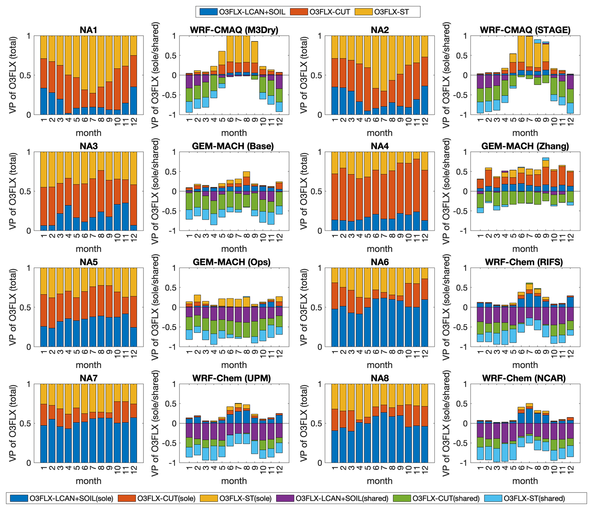
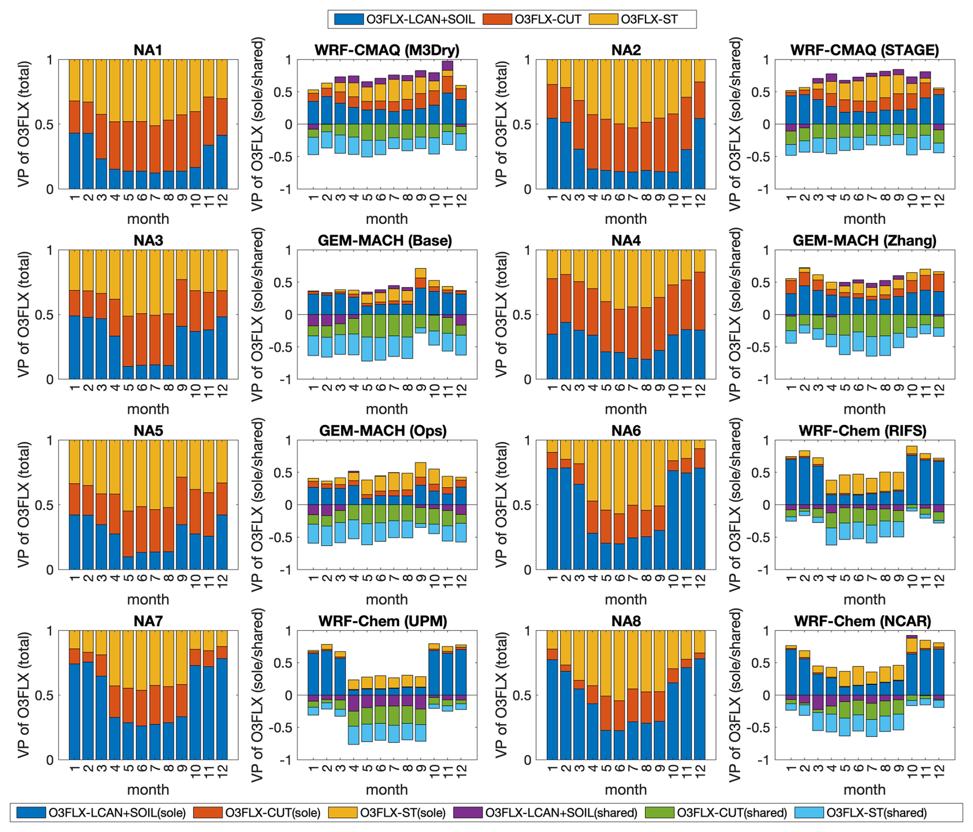
Figure 11 NA case study at 1544 shared cells covered by at least 85 % needleleaf forest. Panels in the first and third column: variance partition (VP) of ozone dry deposition flux into the individual importance (i.e., total effect) of (1) lower canopy and soil effective fluxes combined in one factor, (2) cuticular effective flux, and (3) stomatal effective flux. Panels in the second and fourth column: split of the individual importance of the effective fluxes into sole and shared contributions. The shared effects are displayed with negative numbers. For the sake of making the pictures easier to read, the explicit names of the modeling systems are reported in the figure.

Figure 11 presents the contribution to the ozone dry deposition flux variability of the three effective fluxes (total or “sole” plus “shared”: first and third column of plots in each figure) and their decomposition into “sole” and “shared” fractions (second and fourth column panels) for all months of 2016 and for the eight models participating in the NA case study for shared cells covered by at least 85 % evergreen needleleaf forests.

Considering the first and third columns of Fig. 11 (where the sum of Eqs. 1a and 2b is presented) we note that for all models the fractional contributions to ozone flux variance add up to 1 as expected. For the summer period, we can see that the models can be divided into three main groups. The first group is where stomatal effective fluxes dominate in defining the ozone flux variability (WRF/CMAQ (M3Dry), WRF/CMAQ (STAGE)), a second group where the dominant pathway to ozone flux variability is through the cuticular effective flux (GEM-MACH (Base), GEM-MACH (Ops) and GEM-MACH (Zhang)), and a third group where the main factor is the combined soil and lower canopy effective flux (WRF-Chem (RIFS), WRF-Chem (UPM), WRF-Chem (NCAR)). This constitutes a significant result that is also in line with those obtained by Clifton et al. (2023) but extends their finding. For example, Clifton et al. (2023) show that different models have very different relative partitioning across effective conductances at individual sites. Our result here suggests that spatial variability in the ozone flux across the same LULC type is mainly determined by different flux pathways. Given the fact that the grid cells selected were dominated by the same land use type, differences between the three groups can be attributed to substantial differences in the dry deposition modules, concentration gradients, and meteorology. In the winter and autumn months, the contribution to ozone flux variability is equally distributed across the three pathways for all models for this LULC type. We also note that the seasonal cycle of the “sole” terms varies as a function of model. The stomatal conductance term dominates the CMAQ implementations (NA1, NA2) in the summertime, while for the GEM-MACH implementations (NA3, NA4, NA5), summertime seasonality is mostly driven by the soil+lower canopy term, and for WRF-Chem implementations (NA6, NA7, NA8), stomatal and soil+lower canopy terms both have a weak maximum in the summer.

In Fig. 11 the results of the decomposition obtained according to Eq. (2) are independently presented (columns 2 and 4). For the sake of presenting the results in a clearer way, the contributions to the variation obtained from Eq. (2b) are plotted after changing their sign to better distinguish them from the others, but the total sum of the negative and positive values should be 1. This more detailed analysis allows us to verify the previous one with additional details. For example, the predominance of stomatal flux in WRF-CMAQ in the warm season is due to the sole contribution of stomatal flux, whereas in the other seasons the shared contributions dominate. For GEM-MACH, the importance of the cuticular flux seen earlier arises from its shared contributions except GEM-MACH (Zhang) where its sole fraction appears equally high throughout the year. Five process representation differences between NA3 and NA5 have been summarized above – one of these is different driving meteorology, which may influence differences between these two models in Fig. 11. We note that the WRF-Chem models are also used in feedback mode and have less variation than the GEM-MACH case, potentially indicating a smaller impact of differing model parameterizations on the feedback portions of the WRF-Chem code. Last, for WRF-Chem, the shared contribution of soil and canopy flux is important all year, but its sole contribution becomes equally high in the warm season.

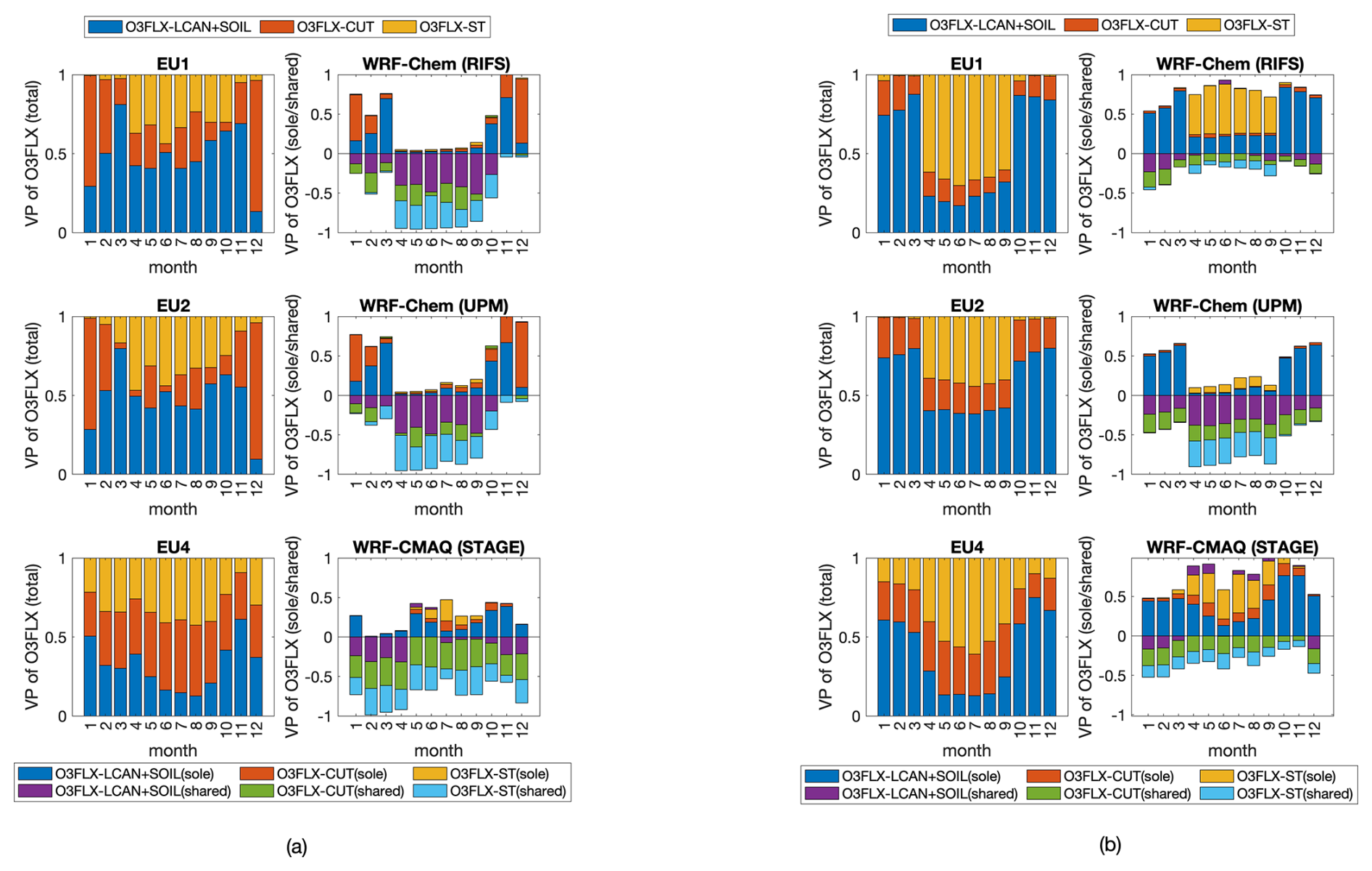
Figure 12 (a) EU case study at 2531 shared cells covered by at least 85 % needleleaf forest. Panels in the first column: variance partition (VP) of ozone dry deposition flux into the individual importance (i.e., total effect) of (1) lower canopy and soil effective fluxes combined in one factor, (2) cuticular effective flux, and (3) stomatal effective flux. Panels in the second column: split of the individual importance of the effective fluxes into sole and shared contributions. The shared effects are displayed with negative numbers. For the sake of making the pictures easier to read, the explicit names of the modeling systems are reported in the figure. (b) Same as (a) but at the location of ozone receptors in EU (1551 shared cells).

Figure 12a shows the same analysis for the EU continent where the picture differs from NA, indicating very different meteorological condition between the two regions. This is not unexpected, in that EU meteorology is strongly influenced by the ocean circulation of the Gulf Stream, while the NA meteorology is over a broad region that has a much broader range of conditions in a “continental” climate. In two of the three models (WRF-Chem), the importance of soil–lower canopy and stomatal effective fluxes in the warm season (mid-spring through October) is due to their shared fractions, while the sole contribution of the cuticular effective flux in winter drives the variation of the total O₃ flux. The seasonality of the EU stomatal component is shared with that of NA6, while the EU soil components have a greater degree of seasonality compared to the NA WRF-Chem models. The other model – EU4 (WRF/CMAQ (STAGE)) – shows a more even distribution of the stomatal contribution across the year and a more equal distribution across the three pathways during the year. EU3 is not presented since no data were delivered for effective conductances.

From Figs. S8–S10 one can deduce that the rest of the land covers (deciduous broadleaf forest, mixed forest, planted-cultivated) still exhibit a dominance of stomatal effective flux during the summer. These LULCs all have a significant deciduous component, and the summertime dominance is in part due to the wintertime absence of foliage in the more northerly parts of the model domains. Depending on the model, cuticular and soil are at times the second contributor to variability of ozone flux.

Figure 13 Same as Fig. 11 but at the location of ozone receptors in NA (1551 shared cells).

The category “ozone receptor” groups the results at grid cells containing an ozone sampling location regardless of the land cover adopted by individual models (Fig. 12b for EU and Fig. 13 for NA). It is interesting to note that the ozone receptor case shows a remarkable consistency across models in terms of the contribution of the different effective fluxes and their variability in time, a behavior not seen when performing this analysis for grid cells dominated by specific LULC types. This can be appreciated from Fig. 12 where the evergreen needleleaf forest case (Fig. 12a) is presented side by side with the ozone receptor case (Fig. 12b) for the EU domain. There is some disagreement for the EU about the stomatal flux contribution during winter (zero or low) and on the exact partitioning during warm months, but generally all the models show substantial contributions from the stomatal flux though disagreeing on the exact non-stomatal partitioning. The consistency for the ozone receptor case is also visible across the continents (Fig. 13 for the NA case) where the contribution has a remarkable resemblance across models for seasonality and the partitioning of the ozone flux variance across the effective fluxes compared to individual land use type values. For the NA case, models suggest moderate to strong contributions for LCAN + SOIL during winter yet small to moderate contributions during summer; the contribution of cuticular effective flux tends to be constant and moderate throughout the year, with three models (WRF-CHEM) suggesting smaller contributions in winter; stomatal effective flux makes up the difference, roughly a third of the total but sometimes as low as 10 % or as high as 50 %.

This result calls for some important considerations.

1. The remarkable consistency and similarity found among the model results at the ozone receptor locations could be due to the lack of dominance of any specific LULC type at this subset of grid cells considered. This would be in agreement with the fact that the locations have presumably been chosen for air quality monitoring activities and by design are intended to be neutral to any prevailing process such as the removal of pollutants from the atmosphere by dry deposition processes, thus extending the spatial representativity of the monitoring locations.

2. The variance decomposition into contributions of both sole fluxes and shared fluxes (columns 2 and 4 of Fig. 13 and column 2 in Fig. 12b) does not show the same agreement found for the total fluxes (columns 1 and 3 of Fig. 13 and column 1 of Fig. 12b). This indicates that every dry deposition model maintains a peculiarity in its behavior for individual land use types. This specificity is lost in the results when the ozone monitoring stations are considered. This suggests that while the monitoring station locations show that the models perform in a similar fashion for mixtures of LULC types, the model performance for individual land use types (represented by a much smaller number of stations) may differ significantly. Given that model performance is judged using observation station values, this may indicate that dry deposition algorithms have been inadvertently tuned towards providing similar results in the regions where mixtures of LULC values are present – but require single LULC type stations for the evaluation of individual LULC performance. We note that this tuning is not intentional but a product of the purpose for which monitoring stations have been set up (e.g., human health impacts and hence closer to human habitations than remote locations which may have a single LULC) and the availability of infrastructure (roads, electrical power) for station operations. This result underscores the importance of land-use-specific dry deposition sites such as those used in point model dry deposition velocity analysis in Clifton et al. (2023, this issue) when evaluating dry deposition algorithms and suggests that subsets of monitoring network stations located in single LULC types should be identified (or constructed if none are available) in order to further improve model performance within those LULC types. The result is that the dry deposition algorithms achieve similar results for dry deposition flux relative to observations – but sometimes via very different pathways, especially across different LULCs. This is in line with suggestions from recent work examining a single model (Silva and Heald, 2018), a review paper on modeling ozone dry deposition (Clifton et al., 2020a), and the results of the single-point modeling AQMEII Activity 2 paper (Clifton et al., 2023). These findings and the above analysis illustrate

   • a strong need to generate observational datasets which focus on specific dry deposition components for model evaluation (e.g., as suggested by Clifton et al., 2020a),

   • the need for dry deposition velocity observation to evaluate dry deposition algorithm performance, and

   • the need for monitoring network locations that represent specific LULCs to improve model performance in regions where one LULC dominates.

   The current evaluation practice with mixed LULC monitoring stations used for dry deposition algorithm evaluation prevents progress in algorithm improvement in specific LULCs and allows LULC-specific compensating errors to be missed in dry deposition algorithm development.

3. If (1) and (2) can be confirmed one should consider comparing dry deposition results obtained at operational monitoring sites with care – the net results of the comparison may be that the regional models and possibly their dry deposition fluxes agree on average for regions with multiple land use types, but the agreement is the result of regional model evaluation procedures as opposed to a mechanistic dry deposition velocity algorithm evaluation that is LULC-specific. Furthermore, this may give an appearance of agreement among regional models that may be illusory, since in grid cells with shared dominant LULC types more disagreement has been demonstrated in the above analysis. An important implication of this finding is the need to evaluate regional models using both single-land-use and multiple-land-use stations in the future and for representation in single-land-use locations to be a consideration in monitoring network design.

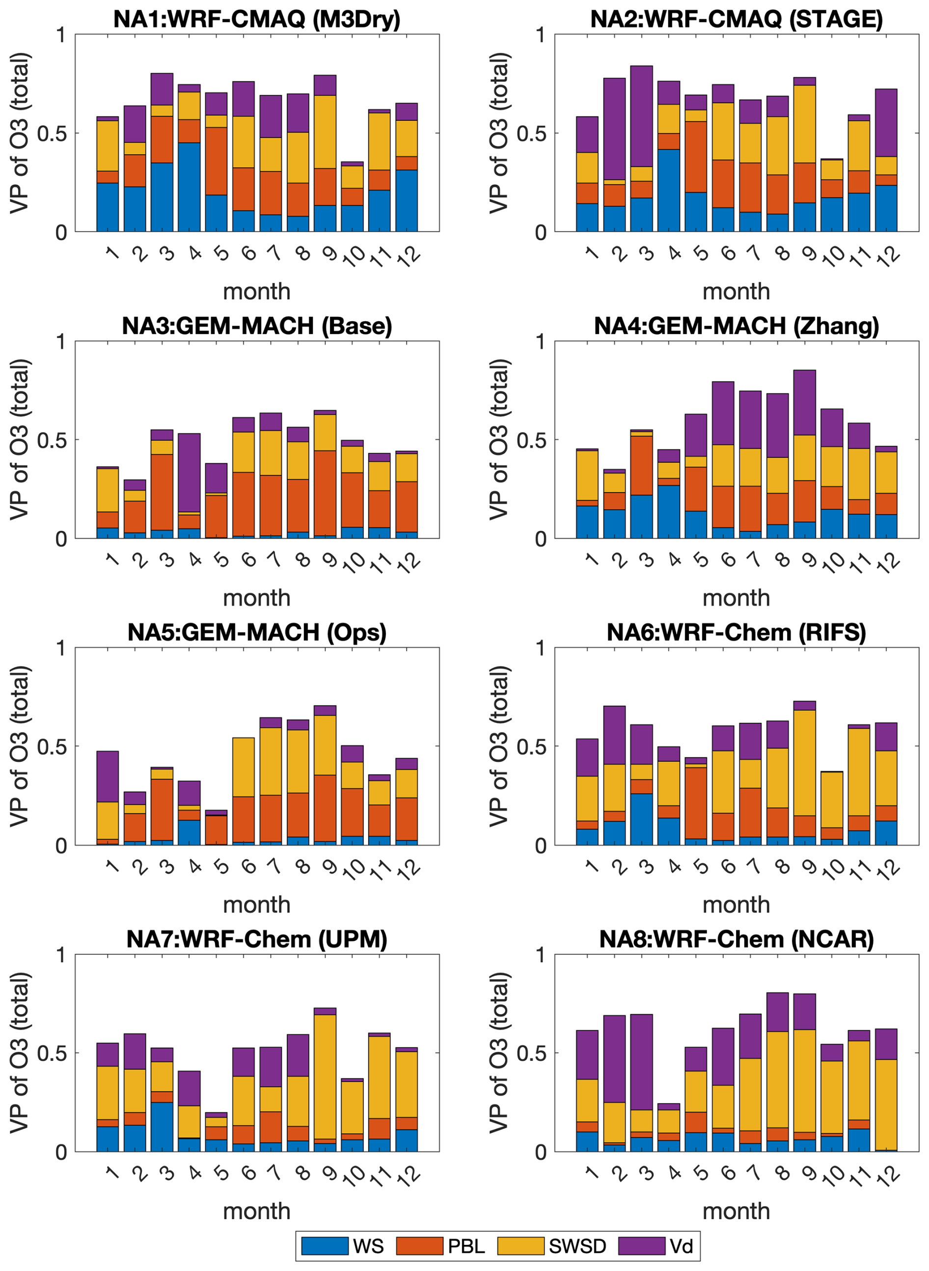
Figure 14 NA case study at 1544 shared cells covered by at least 85 % needleleaf forest. Variance partition (VP) of ozone concentration for each model into the individual importance (i.e., total effect) of wind speed, PBL height, solar radiation, and dry deposition velocity. For the sake of making the pictures easier to read, the explicit names of the modeling systems are reported in the figure.

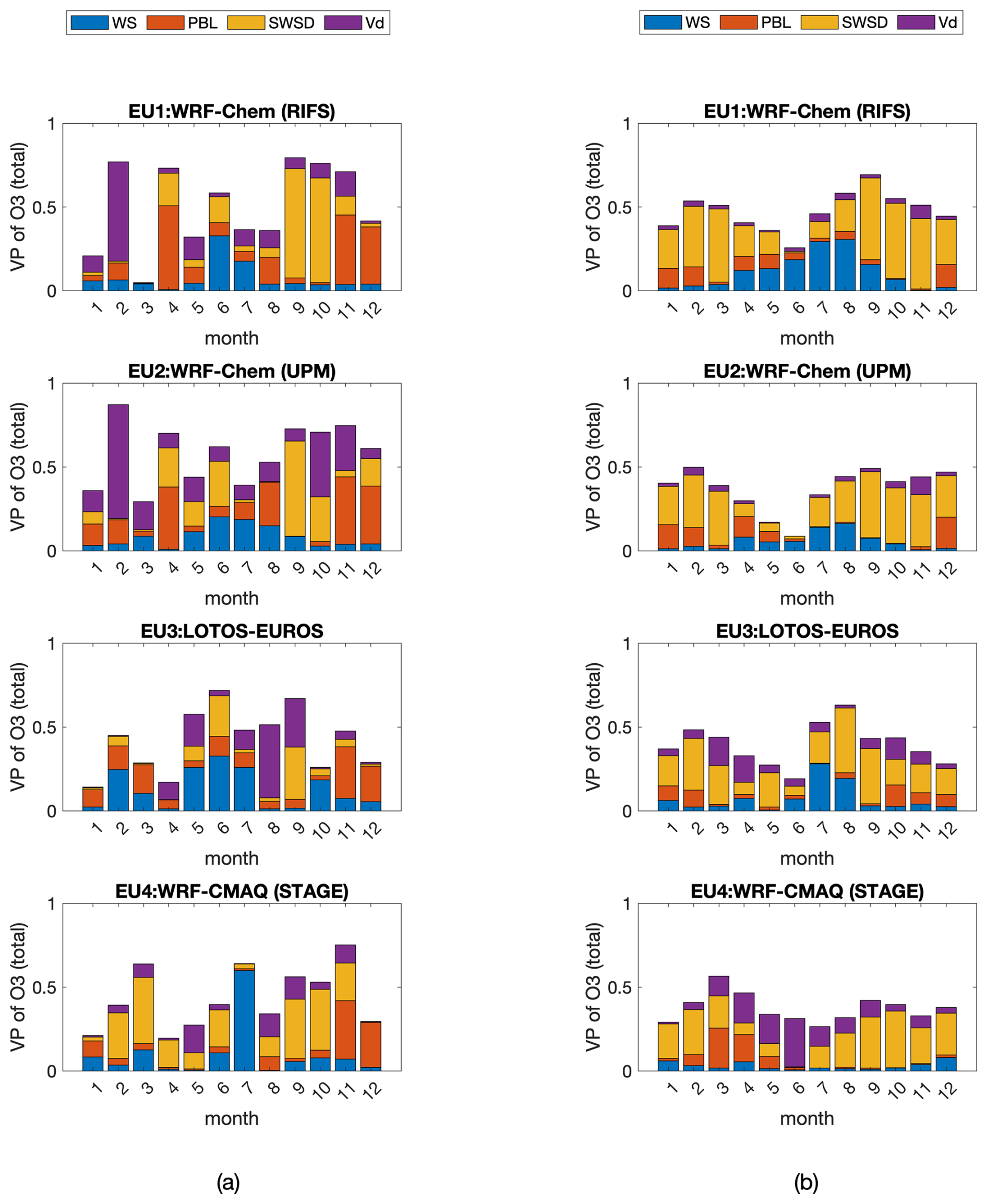
Figure 15 (a) EU case study at 2531 shared cells covered by at least 85 % needleleaf forest. Variance partition (VP) of ozone concentration for each model into the individual importance (i.e., total effect) of wind speed, PBL height, solar radiation, and dry deposition velocity. For the sake of making the pictures easier to read, the explicit names of the modeling systems are reported in the figure. (b) Same as (a) but at the location of the ozone receptors in EU (1551 shared cells).

5.2 Nonlinear contributions of other factors to the ozone concentration variance

The analysis of the nonlinear contributions to the ozone variance has been conducted by introducing other factors considered to be relevant in influencing ozone variability at the surface level, namely boundary layer height, solar radiation, wind speed, and dry deposition velocity. In a way, this analysis allows us to determine the role of dry deposition in relation to other factors influencing the variation of ozone concentrations at the evergreen needleleaf forest cells and therefore estimate its relevance as a driver of ozone variance in a regional-scale model. Figure 14 presents the analysis for the NA case, while Fig. 15 shows results for the EU case.

From Fig. 14 we firstly note that the selected components have a very relevant role in the determination of the surface ozone variance as, overall, they account on average for 60 % to 80 % of ozone variance. The remaining portion can be attributed to variations in emissions and chemical reactions that cannot easily be represented by a specific variable or to other factors not considered in this analysis. Across the eight models participating in the NA case study, we can note the dominance of solar radiation followed by PBL height and dry deposition velocity, whereas wind speed seems to be relevant throughout the year only for three of the eight (WRF/CMAQ (M3Dry), WRF/CMAQ (STAGE), GEM-MACH (Zhang)). We note that correlation does not necessarily imply causation – the wind speed dependence effects noted here may reflect model dependence on the friction velocity, which can be expressed as a function of the wind speed, logarithmic profile, and surface roughness. The contribution of wind speed across models is very scattered in time though contributing on average 30 % of the resolved variability. In some models it appears to be among the dominant factors in winter more than in summer (WRF/CMAQ (M3Dry), WRF/CMAQ (STAGE), GEM-MACH (Zhang), WRF-Chem (RIFS), WRF-Chem (UPM)). While WRF-Chem (UPM) uses the CBMZ mechanism (see Makar et al., 2025, this issue), the dry deposition implementation for CBMZ accounts only for four seasons, while the other two WRF-Chem models (RIFS and NCAR) employ the MOZART chemical mechanism, for which the dry deposition algorithm has tabulated entries on a monthly basis which are used in dry deposition. That is, the WRF-Chem dry deposition implementations which are linked to different gas-phase mechanisms have differing degrees of seasonal resolution.

We note that the differences noted above for NA3 versus NA5 include different LAI information (with different sources and seasonal dependence).

It appears that in North America a seasonality in the contribution of the various components is more evident. The differences between GEM-MACH (Base) and GEM-MACH (Ops) can be attributed at least partially to the meteorology change associated with feedbacks, but also may partially result in the differing seasonality in LAI inputs. The no-feedback model (GEM-MACH (Ops)) has less ozone variability associated with wind speed and more with solar radiation compared to the feedback model GEM-MACH (Base); feedbacks exacerbate meteorological variability. GEM-MACH (Base) versus GEM-MACH (Zhang) shows how much the dry deposition scheme can affect the variability via the feedbacks: GEM-MACH (Base) and GEM-MACH (Zhang) are otherwise identical models. This quantifies the impact of feedbacks on meteorology and hence dry deposition velocity variance. WRF-Chem is also a feedback model, and the impact of the feedbacks shows up as differences in the relative importance of meteorology versus ozone dry deposition velocity itself between the different implementations.

Figure 16 Same as Fig. 14 but at the location of ozone receptors in NA (1551 shared cells).

In EU we see from Fig. 15a that the contributions have a greater degree of scatter than for NA. WRF-Chem (UPM) and WRF/Chem (RIFS) share an important contribution of dry deposition velocity in February and of PBL in April, November, and December. It is interesting that across the year the components account for a smaller portion of the total variance (< 50 %) than in the NA case. This could be due to drastically different conditions and the dominance of emissions variability (and consequently chemistry) for the ozone variability. Each of the models uses different driving meteorology, but the variation in observed conditions across EU may be less than across NA, as noted above. The March case of WRF-Chem (RIFS) is particularly interesting where the PBL height, solar radiation, wind speed, and dry deposition velocity contribute less than 5 % of the ozone variance. Another difference between the NA and EU case studies is the contribution of dry deposition compared to the other processes in determining ozone variability. In NA, dry deposition velocity contributes 10 % to 25 % to ozone variability during summer and 10 % to 50 % during winter. In the EU, however, the summer contribution is much lower and in February two models out of four show a 70 % contribution.

All these results clearly point toward the relevance of dry deposition in determining ozone variability and concentrations at the surface, and yet they also show that important differences are present in the process description in individual models that can greatly influence the outcome.

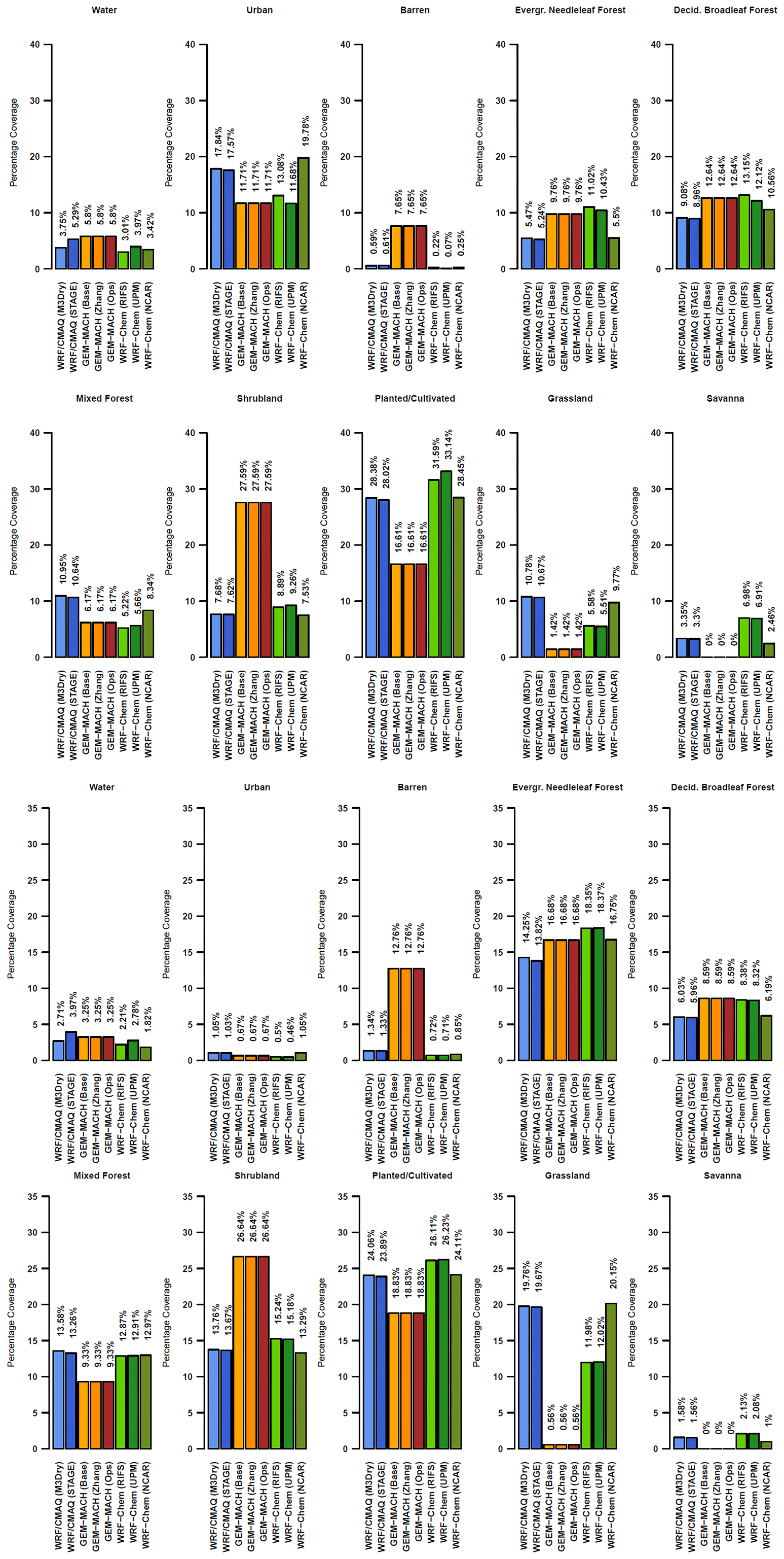
Figure 17 (a) Fraction of entire NA common domain (excl. grid cells dominated by water, i.e., water fraction > 0.5) covered by each LU type. (b) Fraction of all grid cells corresponding to O₃ receptor locations covered by each LU type.

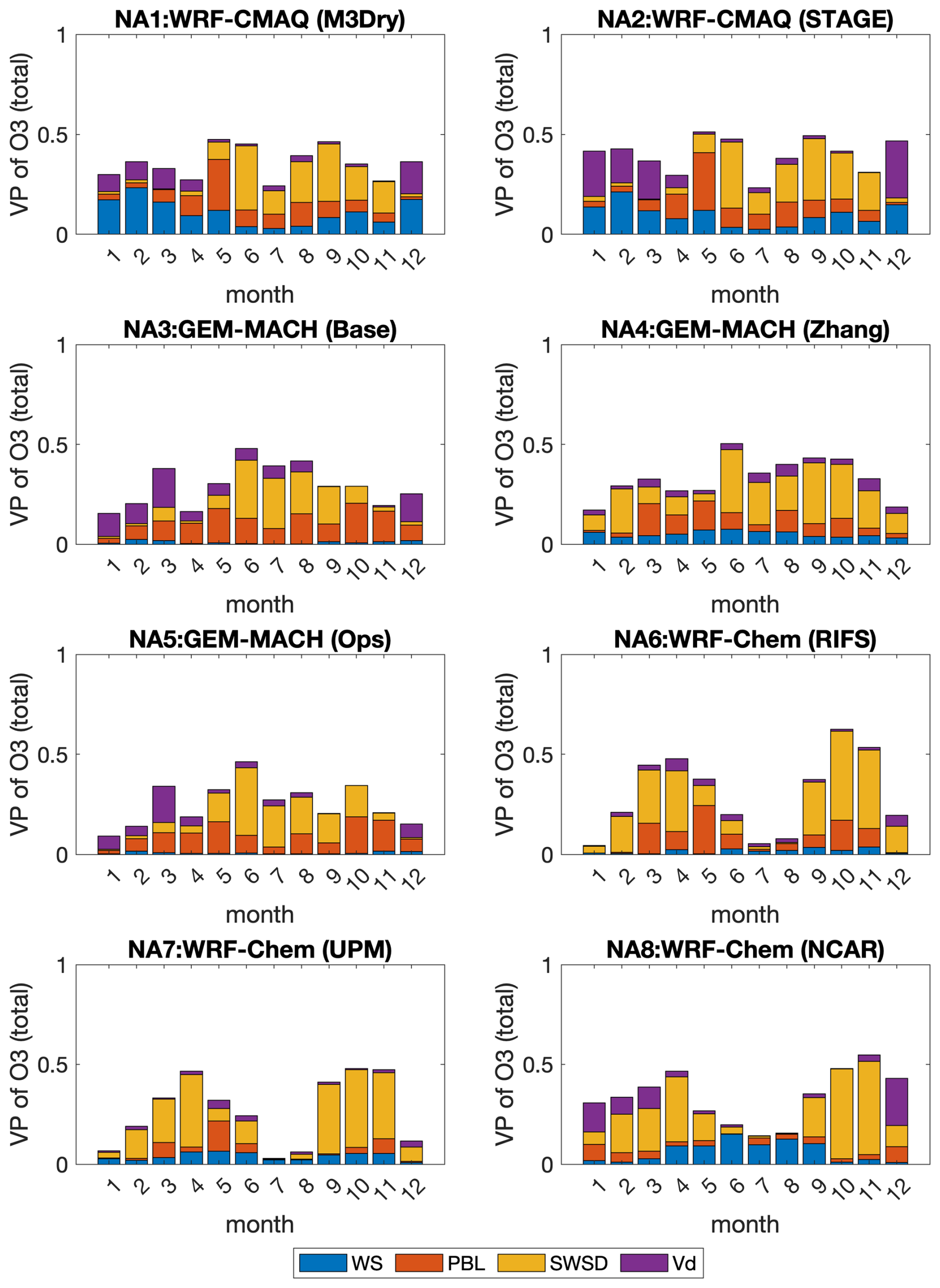
When the same analysis is performed at the O₃ receptor cells, we can clearly demonstrate hypothesis (1) and possibly (2) presented in the previous section. Figure 15b for the EU case and Fig. 16 for the NA case show the results for the O₃ receptor cells. The eight models in the NA case clearly show that at those grid cells the contribution of dry deposition velocity to ozone variability is generally much smaller compared to the results for grid cells with specific common LULC types, for example with respect to evergreen needleleaf forests. Despite this general trend, NA1, NA2, NA3, and NA5 (WRF/CMAQ (M3Dry), WRF/CMAQ (STAGE), GEM-MACH (Base), GEM-MACH (Ops), respectively) still show that during winter, dry deposition can be a significant contributor to ozone concentration variability at receptor locations. This result also confirms hypothesis (3) in the previous section; the operational ozone monitoring sites are not suitable for the analysis of dry deposition results for specific LULC classes. A similar conclusion can be drawn for the EU case (Fig. 15b), which is presented back to back with the evergreen needleleaf forest case. To corroborate the last statement, Fig. 17 shows a comparison of the fraction of the entire NA common domain (excluding grid cells dominated by water, i.e., water fraction > 0.5) covered by each LU type to the LU distribution of all grid cells corresponding to O₃ receptor locations (EU results are shown as Fig. S11). As can be noted, existing O₃ receptor locations are characterized mainly by planted/cultivated, shrubland, and urban LULC with a 10 % coverage of deciduous broadleaf forest (Fig. 17b). At these locations all models appear to have the same distribution of the main LULC type apart from shrubland (NA3, 4, and 5, 20 % more abundant) and planted/cultivated (same models, 10 % less abundant). However, the distribution of LULC from the overall NA common model domain (Fig. 17a) demonstrates that the current receptor site LULC poorly represents the relative amount of land use occurring throughout the domain, with, for example, much higher evergreen needleleaf and grassland fractions and much lower urban land use LULC in the all-domain data of Fig. 17a compared to the observing station values of Fig. 17b.

In this respect, it is important also to note that in spite of the formal differences among dry deposition modules (Galmarini et al., 2021), in conditions of uniform LU characteristics and dominance of urban and planted/cultivated LULC types, the models tend to produce comparable results in terms of contributors to ozone variability. This result further underlines the importance of a correct and uniform characterization of the both the input LULC data and the extent to which monitoring station data reflect LULC across the domain, both of which are driving factors in determining the differences among dry deposition modules.

6 Conclusions

An operational evaluation has been conducted on the models that took part to the AQMEII-4 activity (Galmarini et al., 2021). A total of 12 models were analyzed, 8 of which were run over the North American continental air quality simulation of the year 2016, and the rest were run over Europe for the year 2010. The scope of the evaluation is to determine the level of agreement of the models against available measurements and how they compare with one another. This is normally referred to as operational evaluation and according to Dennis et al. (2010) is the first necessary step prior to any more detailed evaluation or intercomparison of model results. The focus of the fourth phase of AQMEII is the analysis of the performance of dry deposition schemes in regional-scale models, and therefore the operational evaluation has been performed having that goal in mind. Ozone dry deposition, in particular, is the focus of this analysis. Ozone average annual concentration errors ranged between 10 % and 30 % in NA and between 10 % and 15 % in EU except for one model (35 % error). Errors for NO and NO₂ were on the order of 5 %–10 % and 10 %–15 %, respectively, in NA and 15 % for both pollutants in EU. The subregional analysis confirmed these findings, considering the expected subregional variability related to different emission patterns. The models can be distinctively grouped by performance with WRF/CMAQ (M3Dry), WRF/CMAQ (STAGE), GEM-MACH (Base), and GEM-MACH(Ops) showing a better overall capacity to predict ozone concentrations in NA followed by GEM-MACH (Zhang) and WRF-Chem (RIFS), while WRF-Chem (RIFS) and WRF-Chem (NCAR) show larger errors throughout the year and the domain. In the EU case LOTOS/EUROS outperforms the two WRF-Chem versions (RIFS and UPM) and WRF/CMAQ (STAGE). This result is also very evident from the probabilistic analysis where all combinations of possible ensembles were calculated and reflect the results of the operational evaluation.

As far as the dry deposition is concerned, a diagnostic evaluation was performed aiming at analyzing the variance contribution of the different pathways to the variance of the overall ozone dry deposition fluxes. All cells covered with at least 85 % of the same land use types were considered in this analysis. Across grid cells containing mostly needleleaf forests over NA, the main example used in our study, the analysis shows the mixed response of the various dry deposition schemes adopted in the regional-scale models; one group of models shows a prevailing contribution of the stomatal effective flux in determining spatial ozone flux variability, one shows that the three pathways contribute rather equally, and the last group of models shows that the lower canopy and soil effective flux are the prevailing contributors. Thus, models are simulating very different drivers of ozone flux variability in space, even for the same land use type. The contribution to ozone variability of wind speed, dry deposition velocity, solar radiation, and boundary layer height was also investigated.

When the abovementioned analysis was also performed for all grid cells where ozone monitors were present regardless of the LULC type, a remarkable result was found. Regardless of the EU or NA case considered, all the differences among models found for specific LULC types largely disappeared, showing a more uniform behavior across models. This aspect was demonstrated to be attributable to a minor contribution of dry deposition at those sites in determining the ozone variability when compared with other factors. Other factors contributing to this behavior are the presence of predominant LULC types for which dry deposition is relatively low and the uniform distribution of those types and other LULC types across the models at the observation station locations.

This result allows us to present important conclusions. The first conclusion is that the evaluation of dry deposition processes should not be conducted only at operational ozone monitoring sites. The latter's characteristics are selected based on other considerations aside from dry deposition. They appear unsuitable for dry deposition algorithm evaluation. An analysis of dry deposition modeling at these sites may produce illusory agreement among models that could be completely misleading and misrepresentative. Therefore, specific sites with a predominance of LULCs which induce high dry deposition should be selected among existing monitoring stations, or added to existing monitoring networks, for dry-deposition-focused model evaluation.

The second conclusion is a recurring theme throughout AQMEII-4 regional modeling studies to date (e.g., Hogrefe et al., 2025; Makar et al., 2025), namely the necessity of a harmonization of LULC data across regional-scale air quality models, as large diversity in the characterization of the surface is still present among all models, and this diversity has a significant impact on model performance. Considering the existence of detailed information in space and time on LULC (e.g., Copernicus Land Monitoring services, USGS, Landsat), we find the lack of agreement between models on the input land use data anachronistic and of great concern. Any interpretation of the behavior of dry deposition schemes will be impaired by the lack of agreement of LULC masks and will inevitably include an inherent uncertainty difficult to quantify. The present situation is comparable to the one where models use different topographies or terrain elevations to the extent of including (excluding) specific reliefs or mountain ranges in (from) the domain. If there is an ambition to improve the performance of regional-scale models in terms of dry deposition processes (effectively a sink in the concentration budget), the selection of up-to-date and common LULC data is a fundamental and necessary prerequisite. Considering the advances in the characterization of land surface at very high spatial and temporal resolutions (meter scale), such effort cannot be further delayed and should be taken on prior to any new model evaluation or intercomparison of dry deposition processes.