Effects of ozone–climate interactions on the long-term temperature trend in the Arctic stratosphere

Using reanalysis datasets and the Community Earth System Model (CESM), this study investigates the effects of ozone–climate interactions on the Arctic stratospheric temperature (AST) changes during winter and early spring. Before 2000, the AST increased significantly in early winter (November and December), which is contributed to by ozone–climate interactions. Specifically, ozone–climate interactions lead to a stratospheric state that enhances upward wave propagation and the downwelling branch of Brewer–Dobson circulation. This leads to an adiabatic warming that significantly raises the AST. This dynamical heating overwhelmingly offsets the longwave radiative cooling effect associated with increased ozone during early winter. In contrast, during late winter and spring, cooling trends in the Arctic stratosphere are predominantly driven by reduced shortwave radiation heating associated with stratospheric ozone depletion. This study highlights the effects of ozone–climate interactions on the long-term trend in the AST.

1 Introduction

The stratospheric ozone layer plays an important role in global climate change (Son et al., 2008; Smith and Polvani, 2014; Xia et al., 2016; Xie et al., 2018; Hu et al., 2019a; Sigmond and Fyfe, 2014; Chiodo et al., 2021; Ivanciu et al., 2022; Friedel et al., 2023). Its absorption of solar ultraviolet radiation, along with its strong infrared radiation absorption and emission around the 9.6 µm band, is crucial for the Earth's energy balance and the thermal structure of the atmosphere (de F. Forster and Shine, 1997). The annual global mean radiative forcing of stratospheric ozone during the strongest ozone depletion period (1979–1996) is relatively small (−0.22 ± 0.03 W m⁻²; de F. Forster and Shine, 1997) compared to that of CO₂ (2.16 ± 0.25 W m⁻²; IPCC, AR5, 2014). However, in addition to the direct radiative forcing mentioned above, stratospheric ozone can also significantly affect atmospheric temperature through ozone–climate interactions, which involve chemical–radiative–dynamical coupling processes (Dietmüller et al., 2014; Nowack et al., 2015). For instance, neglecting interactive stratospheric chemistry and considering only the direct radiative effect of ozone in climate models results in a 20 % overestimation of surface temperature in scenarios with quadrupled CO₂ concentrations (Nowack et al., 2015). A similar overestimation of surface temperatures can also be found in the study of Chiodo and Polvani (2016). In addition, Rieder et al. (2019) demonstrated that ozone–climate interactions are important for accurately capturing stratospheric temperature variability in models. However, some studies, such as Marsh et al. (2016), suggested that ozone–climate interactions have limited influences (approximately 1 %) on climate sensitivity. Therefore, whether the ozone–climate interactions have significant influence on temperature variability is still unclear.

Ozone–climate interaction is complex, especially in the polar stratosphere. It involves different feedback mechanisms that vary across seasons. In winter, although solar radiation in the Arctic regions is absent, ozone can still absorb and emit longwave radiation. Seppälä et al. (2025) pointed out that a reduction in stratospheric ozone could directly lead to stratospheric warming. This longwave radiative warming may influence the strength of the Arctic polar vortex (Hu et al., 2015), further modulating the transport of ozone-rich air from mid-latitudes to the Arctic polar regions (Zhang et al., 2017). Moreover, the Arctic stratospheric ozone can modulate planetary wave activity, which further influences Arctic stratospheric temperature (AST) via wave-mean flow interactions in winter (Nathan and Cordero, 2007; Albers and Nathan, 2013; Hu et al., 2015). McCormack et al. (2011) pointed out that the presence of ozone–climate interactions gives rise to a climatologically weaker, warmer and more disturbed polar vortex during Arctic winter. In late February and early spring, as solar radiation reaches high latitudes, the polar regions become warm compared to the winter period and the stratospheric polar vortex is weakened. However, from the perspective of climate, the increase in ozone depleting substances (ODSs) in the twentieth century leads to springtime stratospheric ozone depletion and decreased absorption of shortwave radiation, which cools the Arctic stratosphere and strengthens the polar vortex compared to the climatological mean (Friedel et al., 2022a). This results in reduced wave propagation towards the lower stratosphere and thereby a colder Arctic stratosphere than normal (Coy et al., 1997; Albers and Nathan, 2013; Haase and Matthes, 2019). On one hand, the strengthened Arctic polar vortex decreases ozone transport to the polar regions, further reducing ozone concentrations. On the other hand, a colder Arctic stratosphere facilitates the formation of polar stratospheric clouds (PSCs). PSCs provide sites for heterogeneous reactions. The reactions convert stable chlorine reservoir species into active chlorine, then catalytically destroys ozone during spring (Solomon et al., 1986; Feng et al., 2005a, b; Calvo et al., 2015). Therefore, ozone–climate interactions in winter and spring involve different and complex chemical–radiative–dynamical feedback processes, which operate on different time scales (Tian et al., 2023).

The Arctic climate plays a crucial role in the global climate system, and its temperature changes have profound implications for global climate patterns (Cohen et al., 2014; Serreze and Barry, 2011; Overland et al., 2016). In recent decades, the Arctic long-term temperature trends are not only driven by a range of external factors such as sea ice, greenhouse gas emissions (GHGs) and aerosols (IPCC, AR6, 2021; Shindell and Faluvegi, 2009; Screen and Simmonds, 2010), but are also influenced by natural variability in the climate system. During the period from 1950 to 2000, in late winter, a negative trend in stratospheric temperature is observed in the Arctic regions, which is associated with the weakening of wave activity (Randel and Wu, 2002; Zhou et al., 2001; Hu and Tung, 2003). However, the temperature trends in early and mid-winter (November–January) are opposite to those in late winter from 1980 to 2000 (Bohlinger et al., 2014; Young et al., 2012). Most previous studies focused only on the role of dynamical processes in the seasonal difference in temperature trends (Newman et al., 2001; Hu and Fu, 2009; Young et al., 2012; Ossó et al., 2015; Fu et al., 2019). However, these long-term trends in Arctic temperatures are not fully explained by dynamical processes. Recent work by Chiodo et al. (2023) explored the effect of long-term ozone trends on the temperature in the Arctic, providing valuable insights into the ozone–climate interactions. Notably, the Arctic ozone layer has also undergone significant changes over the past 40 years (WMO, 2018). The ozone layer has been significantly depleted since the late 1970s (Farman et al., 1985) and has been recovering slowly since 2000 as ODSs have decreased (WMO, 2018, 2022; Chipperfield et al., 2017). In addition, the influence of ozone–climate interactions on temperature in the polar regions differs across seasons (Tian et al., 2023). Therefore, it is worth investigating whether Arctic ozone trends and their climate interactions can explain the long-term trends in Arctic temperature across different seasons.

This study focuses on the historical long-term trends in the AST during winter and spring, with a particular emphasis on the role of ozone–climate interactions. Specifically, we seek to answer the following questions: (1) What are the observed trends in AST and ozone concentrations over recent decades? (2) How do ozone–climate interactions contribute to these trends? (3) What mechanisms drive the seasonal differences in these trends? By addressing these questions, this study aims to enhance our understanding of the role of ozone–climate interactions in long-term Arctic stratospheric changes and their implications for future climate projections. Section 2 outlines the data, methodologies and climate model experimental designs employed in this study. Section 3 presents the observed trends in temperature and ozone concentrations over the Arctic stratosphere, and Sect. 4 explores the underlying physical processes. Finally, Sect. 5 summarizes the conclusions and discusses future directions.

2 Data, methods and experimental configurations

2.1 Data

The European Centre for Medium-Range Weather Forecasts (ECMWF) v5 reanalysis dataset (ERA5; Hersbach et al., 2020) from 1980 to 2020 is used in this study. The horizontal resolution of this dataset is 1° × 1° (latitude × longitude) and there are 37 vertical levels ranging from 1000 to 1 hPa. The daily and monthly mean results are derived from the three-hourly ERA5 reanalysis dataset. We also used daily meteorological data obtained from the NASA Modern-Era Retrospective Analysis for Research and Applications version 2 (MERRA2) product (Gelaro et al., 2017), which has a horizontal resolution of 1.25° × 1.25° (latitude × longitude), and 42 pressure levels in the vertical direction extending from 1000 to 0.1 hPa from 1980 to 2020. The meteorological fields used in this study include daily mean horizontal winds, temperature, geopotential height and ozone.

2.2 Methods

2.2.1 Diagnosis of wave activity

Eliasson–Palm flux

The Eliasson–Palm (E–P) flux (Andrews et al., 1987) is used to diagnose the propagation of waves in the vertical and meridional directions and is calculated as follows:

$$\begin{array}{}\text{(1)}& {\displaystyle }F\mathit{\varphi }\equiv {\mathit{\rho }}_{\mathrm{0}}a\cos \mathit{\varphi }\left({\displaystyle \frac{\stackrel{\mathrm{‾}}{uz}\stackrel{\mathrm{‾}}{v^{\prime }{\mathit{\theta }}^{\prime }}}{\stackrel{\mathrm{‾}}{\mathit{\theta }z}}}-\stackrel{\mathrm{‾}}{u^{\prime }{v}^{\prime }}\right),\text{(2)}& {\displaystyle }Fz\equiv {\mathit{\rho }}_{\mathrm{0}}\cos \mathit{\varphi }\left\{\left[f-{\left(a\cos \mathit{\varphi }\right)}^{-\mathrm{1}}\left(\stackrel{\mathrm{‾}}{u}\cos \mathit{\varphi }\right)\mathit{\varphi }\right]{\displaystyle \frac{\stackrel{\mathrm{‾}}{v^{\prime }{\mathit{\theta }}^{\prime }}}{\stackrel{\mathrm{‾}}{\mathit{\theta }z}}}-\stackrel{\mathrm{‾}}{w^{\prime }{u}^{\prime }}\right\},\text{(3)}& {\displaystyle }\mathrm{\nabla }\cdot \overrightarrow{F}\equiv -\left({\mathit{\rho }}_{\mathrm{0}}\stackrel{\mathrm{‾}}{u^{\prime }{v}^{\prime }}\right)\mathit{\varphi }+\left({\mathit{\rho }}_{\mathrm{0}}f{\displaystyle \frac{\stackrel{\mathrm{‾}}{v^{\prime }{\mathit{\theta }}^{\prime }}}{\stackrel{\mathrm{‾}}{\mathit{\theta }z}}}\right)z,\end{array}$$

where ρ₀ represents the density; z represents the altitude; a represents the radius of the Earth; ϕ represents latitude; f represents the Coriolis parameter; θ represents the potential temperature; u and v represent the zonal and meridional winds, respectively; and w represents vertical velocity. The overbars represent the zonal average, and the primes represent deviations with respect to the zonal average. We ignore the term $\stackrel{\mathrm{‾}}{w^{\prime }{u}^{\prime }}$ because it is small relative to the other terms (Zhang et al., 2019; Zhao et al., 2022).

Brewer–Dobson circulation

Brewer–Dobson circulation (BDC) is driven by wave breaking in the stratosphere, and BDC in the atmosphere is represented in log-pressure coordinates as follows (Andrews et al., 1987):

$$\begin{array}{}\text{(4)}& {\displaystyle }{\stackrel{\mathrm{‾}}{v}}^{*}\equiv \stackrel{\mathrm{‾}}{v}-{\mathit{\rho }}_{\mathrm{0}}^{-\mathrm{1}}({\mathit{\rho }}_{\mathrm{0}}\stackrel{\mathrm{‾}}{v^{\prime }{\mathit{\theta }}^{\prime }}/{\stackrel{\mathrm{‾}}{\mathit{\theta }}}_z{)}_z,\text{(5)}& {\displaystyle }{\stackrel{\mathrm{‾}}{w}}^{*}\equiv \stackrel{\mathrm{‾}}{w}+\left(a\cos \mathit{\varphi }{)}^{-\mathrm{1}}\right(\cos \mathit{\varphi }\cdot \stackrel{\mathrm{‾}}{v^{\prime }{\mathit{\theta }}^{\prime }}/{\stackrel{\mathrm{‾}}{\mathit{\theta }}}_z{)}_{\mathit{\varphi }},\end{array}$$

where ${\stackrel{\mathrm{‾}}{v}}^{*}$ and ${\stackrel{\mathrm{‾}}{w}}^{*}$ are the zonal-mean meridional and vertical velocities, respectively; θ is the potential temperature; a is the radius of Earth; ϕ is latitude; ρ₀ is the air density; and z is the log-pressure height.

Using the generalized downward control principle, BDC can be further decomposed into different forcing terms (Song and Chun, 2016):

$$\begin{array}{}\text{(6)}& {\displaystyle }\begin{array}{rl}{\stackrel{\mathrm{‾}}{v}}^{*}& =-{\displaystyle \frac{\mathrm{1}}{{\mathit{\rho }}_{\mathrm{0}}\cos \mathit{\phi }}}{\displaystyle \frac{\partial }{\partial z}}\left\{-\cos \mathit{\phi }{\int }_z^{\mathrm{\infty }}{\mathit{\rho }}_{\mathrm{0}}\right.\\ & \left.\left[{\displaystyle \frac{\frac{\mathrm{1}}{{\mathit{\rho }}_{\mathrm{0}}a\cos \mathit{\phi }}\mathrm{\nabla }\cdot F+\stackrel{\mathrm{‾}}{\mathrm{GWD}}+\stackrel{\mathrm{‾}}{X}-\frac{\partial \stackrel{\mathrm{‾}}{u}}{\partial t}}{f-\frac{\mathrm{1}}{a\cos \mathit{\phi }}\frac{\partial }{\partial \mathit{\phi }}\left(\stackrel{\mathrm{‾}}{u}\cos \mathit{\phi }\right)}}\right]\mathrm{d}{z}^{\prime }\right\}\end{array},\text{(7)}& {\displaystyle }\begin{array}{rl}{\stackrel{\mathrm{‾}}{w}}^{*}& ={\displaystyle \frac{\mathrm{1}}{{\mathit{\rho }}_{\mathrm{0}}a\cos \mathit{\phi }}}{\displaystyle \frac{\partial }{\partial \mathit{\phi }}}\left\{-\cos \mathit{\phi }\left[{}_z^{\mathrm{\infty }}{\mathit{\rho }}_{\mathrm{0}}\right.\right.\\ & \left.\left[{\displaystyle \frac{\frac{\mathrm{1}}{{\mathit{\rho }}_{\mathrm{0}}a\cos \mathit{\phi }}\mathrm{\nabla }\cdot F+\mathrm{GWD}+\stackrel{\mathrm{‾}}{X}-\frac{\partial \stackrel{\mathrm{‾}}{u}}{\partial t}}{f-\frac{\mathrm{1}}{a\cos \mathit{\phi }}\frac{\partial }{\partial \mathit{\phi }}\left(\stackrel{\mathrm{‾}}{u}\cos \mathit{\phi }\right)}}\right]\mathrm{d}{z}^{\prime }\right\},\end{array}\end{array}$$

where ∇⋅F, $\stackrel{\mathrm{‾}}{\mathrm{GWD}}$, $\stackrel{\mathrm{‾}}{X}$ and $\partial \stackrel{\mathrm{‾}}{u}/\partial t$ represent the E–P flux divergence, gravity wave forcing, residual term of the transformed Eulerian mean (TEM) equations, and zonal-mean zonal wind tendency, respectively. Song and Chun (2016) reported that the gravity wave drag term $\stackrel{\mathrm{‾}}{\mathrm{GWD}}$ and the residual term $\stackrel{\mathrm{‾}}{X}$ are relatively smaller than the E–P flux divergence and zonal mean zonal wind tendency terms. Therefore, $\stackrel{\mathrm{‾}}{\mathrm{GWD}}$ and $\stackrel{\mathrm{‾}}{X}$ are not considered in this study.

Transformed Eulerian-mean (TEM) formulation

This study uses the TEM formulation of the zonal-mean tracer continuity equation in log-pressure and spherical coordinates in order to accurately diagnose the eddy forcing of the zonal-mean transport of stratospheric ozone. BDC transport is calculated using the first two terms on the right-hand side of Eq. (8), eddy transport is calculated using the sum of the third and fourth terms on the right-hand side (Monier and Weare, 2011; Abalos et al., 2013; Zhang et al., 2017):

$$\begin{array}{}\text{(8)}& \begin{array}{rl}{\displaystyle \frac{\partial {\stackrel{\mathrm{‾}}{\mathit{\chi }}}_{{\mathrm{O}}_{\mathrm{3}}}}{\partial t}}& =-{\displaystyle \frac{{\stackrel{\mathrm{‾}}{v}}^{*}}{R}}{\displaystyle \frac{\partial {\stackrel{\mathrm{‾}}{\mathit{\chi }}}_{{\mathrm{O}}_{\mathrm{3}}}}{\partial \mathit{\varphi }}}-{\stackrel{\mathrm{‾}}{w}}^{*}{\displaystyle \frac{\partial {\stackrel{\mathrm{‾}}{\mathit{\chi }}}_{{\mathrm{O}}_{\mathrm{3}}}}{\partial z}}\\ & -{\displaystyle \frac{\mathrm{1}}{{\mathit{\rho }}_{\mathrm{0}}R}}{\displaystyle \frac{\partial }{\partial \mathit{\varphi }}}\left[{\mathit{\rho }}_{\mathrm{0}}\left({\stackrel{\mathrm{‾}}{v^{\prime }{\mathit{\chi }}^{\prime }}}_{{\mathrm{O}}_{\mathrm{3}}}-{\displaystyle \frac{\stackrel{\mathrm{‾}}{v^{\prime }{\mathit{\theta }}^{\prime }}}{\partial \stackrel{\mathrm{‾}}{\mathit{\theta }}/\partial z}}{\displaystyle \frac{\partial {\stackrel{\mathrm{‾}}{\mathit{\chi }}}_{{\mathrm{O}}_{\mathrm{3}}}}{\partial z}}\right)\right]\\ & -{\displaystyle \frac{\mathrm{1}}{{\mathit{\rho }}_{\mathrm{0}}}}{\displaystyle \frac{\partial }{\partial z}}\left[{\mathit{\rho }}_{\mathrm{0}}\left({\stackrel{\mathrm{‾}}{w^{\prime }{\mathit{\chi }}^{\prime }}}_{{\mathrm{O}}_{\mathrm{3}}}+{\displaystyle \frac{\mathrm{1}}{R}}{\displaystyle \frac{\stackrel{\mathrm{‾}}{v^{\prime }{\mathit{\theta }}^{\prime }}}{\partial \stackrel{\mathrm{‾}}{\mathit{\theta }}/\partial z}}{\displaystyle \frac{\partial {\stackrel{\mathrm{‾}}{\mathit{\chi }}}_{{\mathrm{O}}_{\mathrm{3}}}}{\partial \mathit{\varphi }}}\right)\right]+\stackrel{\mathrm{‾}}{S}\end{array},\end{array}$$

where $\stackrel{\mathrm{‾}}{S}$ is the sum of all chemical sources and sinks, ${\stackrel{\mathrm{‾}}{\mathit{\chi }}}_{{}_{{\mathrm{O}}_{\mathrm{3}}}}$ is the zonal-mean ozone concentration, ${\stackrel{\mathrm{‾}}{v}}^{*}$ and ${\stackrel{\mathrm{‾}}{w}}^{*}$ are the meridional and vertical BDC velocities (Andrews et al. 1987), respectively; ρ₀ is air density; θ is potential temperature; R is Earth's radius; t is time; ϕ and z are latitude and height, respectively.

In Eqs. (1)–(8), the overbar denotes zonal mean, while the prime denotes deviations from the zonal mean; the subscripts indicate partial derivatives. The Fourier decomposition is used to obtain components $u{}^{\prime },v{}^{\prime }$ and θ^′ in Eqs. (1)–(3) and components ∇⋅F in Eqs. (6)–(7) with different zonal wavenumbers.

2.2.2 Statistical methods

The trend is measured by the slope of a linear regression based on a least-squares estimation. We use a two-tailed Student's t test to calculate the significance of the trend or perform a mean difference analysis. This paper measures the results of the significance test with p values or confidence intervals; p≤ 0.1 indicates that the trend or mean difference is significant at/above the 90 % confidence level.

In this study, the normalized time series are standardized using Z-score standardization, where the data are processed using the following formula: $A_{\text{s-value}}=\frac{A_{\text{o-value}}-\stackrel{\mathrm{‾}}{A}}{{\mathit{\sigma }}_A}$, where A_s-value denotes the normalized A-value, A_o-value denotes original A-value, $\stackrel{\mathrm{‾}}{A}$ denotes average A-value, σ_A denotes standard deviation.

2.3 Model and experimental configurations

The F_1955–2005_WACCM_CN (F55WCN) component in the Community Earth System Model (CESM) Version 1.2.2 is used. The F55WCN includes an active atmosphere and land, a data ocean (run as a prescribed component by simply reading sea surface temperature forcing data instead of running an ocean model) and sea ice. The model resolution is 1.9° latitude by 2.5° longitude, with 66 vertical levels and extends from the surface to approximately 5.96 × 10⁻⁶ hPa. The chemistry module in F55WCN calculates the concentrations of different species and includes both gas phase and heterogeneous chemistry in the stratosphere. The physics schemes in the F55WCN are based on those in the Community Atmosphere Model, Version 4 (CAM4; Neale et al., 2013).

To understand the causality of the ozone–circulation coupling, we perform model experiments to isolate the effect of ozone changes on stratospheric dynamics and circulation. Two groups of ensemble climate model experiments (i.e., the control experiment and O3clm experiment) use identical boundary conditions and initial conditions. Each group simulation consists of five ensemble members, with initial temperature conditions randomly perturbed. Both of the two experiments run from 1970 to 2020; the first 10 years are spin-up time. The control experiment uses fully interactive ozone chemistry, and long-term stratospheric ozone changes are involved in the radiation scheme. In contrast, in the O3clm experiment, the climatological mean ozone is represented by monthly three-dimensional mean data from a 1980-clim experiment, which is imported into the radiation scheme. In the 1980-clim experiment, surface emissions, external forcing, stratospheric aerosols, fixed lower boundary conditions and the solar spectral irradiance are all fixed at 1980. The 1980-clim experiment runs for 40 years with the first 10 years as spin-up time and the remaining 30 years of data are used to drive the radiation scheme of the O3clm experiment. This results in the production of fixed radiative feedback, which is to say that the ozone–climate interactions over a long period are not radiatively active. In addition, this setting is designed to preserve the seasonal temperature variations consistent with Earth's background environmental conditions, ensuring the experiment runs stably. Thus, the comparison between the ensemble mean of control and O3clm experiments isolates the feedback effects of long-term stratospheric ozone changes on atmospheric temperature and circulation from climate variability. Figure 1 (adapted from Friedel et al., 2022a, b) provides the conceptual framework for the experimental design, which is crucial to understanding the analysis presented in this study.

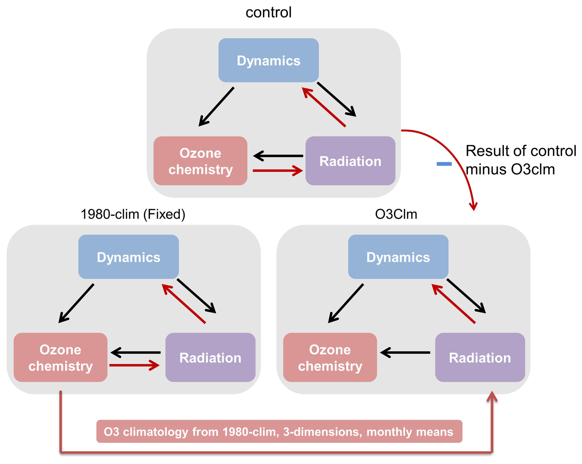
Figure 1 Simulation setup of the ensemble control and O3clm experiments. The control experiment treats ozone chemistry fully interactively. That is, the calculated ozone field has direct feedback on the atmosphere via the model radiation scheme. In contrast, the ensemble O3clm experiments do not use interactively calculated ozone in the radiation module. Instead, the radiation module uses an ozone climatology, which is derived from the 1980-clim experiment (see Sect. 2.3). (This figure is adapted from Fig. 3a in Friedel et al., 2022a, and Fig. 1 in Friedel et al., 2022b.)

3 Trends in temperature and ozone over the Arctic in the middle and lower stratosphere

In this study, we primarily focus on a detailed analysis in the pre-2000 period from 1980 to 2000, during which significant stratospheric ozone depletion occurred (Petropavlovskikh et al., 2019; IPCC, AR6, 2023). The changes after 2000 are briefly discussed at the end of Sect. 4. Figure 2 displays the normalized time series and linear trends of AST (over 65–90° N, 10–150 hPa) during different periods from early winter to early spring. In November–December, the AST exhibits a weak positive trend in the pre-2000 period in both the MERRA2 and ERA5 reanalysis datasets, and it shows an insignificant negative trend after 2000 (Fig. 2a; the black line represents MERRA2, while the gray line represents ERA5). This suggests that there is a warming trend in the Arctic stratosphere during early winter in the pre-2000 period, followed by a cooling trend in the post-2000 period. The ensemble mean of control experiments reproduces these trends well, with a significant positive trend in temperature before 2000 and a significant negative trend after 2000 (Fig. 2a; purple line). From January to February, the temperature displays an insignificant negative trend before 2000 and a significant negative trend after 2000, derived from the three datasets (Fig. 2b). In March–April, the temperature shows a significant negative trend before 2000. After 2000, There is an unremarkable positive trend in MERRA2 and ERA5 datasets and an insignificant negative trend in the ensemble mean of the control experiments (Fig. 2c). Overall, the long-term trends in temperature derived from the ensemble mean of control experiments are nearly consistent with the results from the reanalysis datasets, both in the period before 2000 and after 2000. The reasons for the intra-seasonal opposite temperature trends are investigated in the following section.

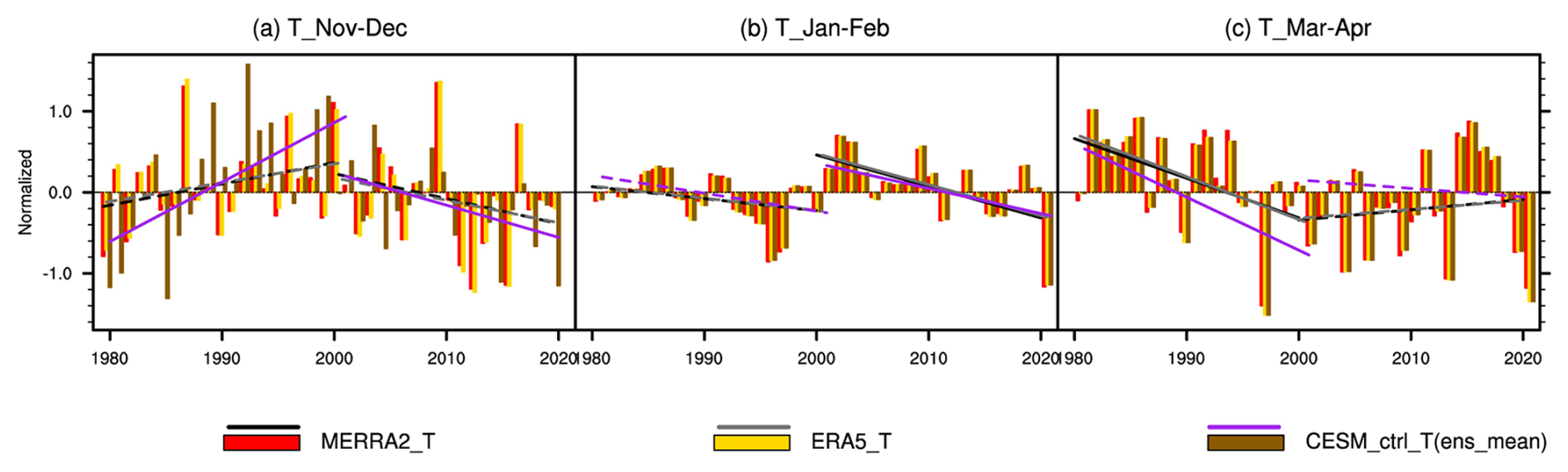
Figure 2 Normalized time series of the temperature averaged from 150 to 10 hPa over 65–90° N from 1980–2020 in (a) November–December, (b) January–February, and (c) March–April derived from MERRA2 (red column), ERA5 (yellow column) and CESM ensemble mean of control experiments (brown column). The color straight lines represent the linear trends before 2000 and after 2000. Solid lines indicate that the trends are statistically significant at the 90 % confidence level according to Student's t test (for details of the normalization method, refer to Sect. 2.2.2: Statistical methods).

Figure 3 shows the trends in daily temperature and ozone between 10 and 250 hPa in the polar cap regions (65–90° N) before 2000, which are based on data from MERRA2 and the ensemble mean of the control experiments. A trend reversal phenomenon is evident at the end of December, which is consistent with Fig. 2. During November and December, there are positive temperature trends across all levels and increasing ozone in the upper stratosphere (Fig. 3a, b). While, after December, the trends in temperature and ozone reverse in the middle stratosphere and then in the lower stratosphere. Similar trend patterns are found in the ensemble control experiments (Fig. 3c,d), with more significant positive trends in temperature and ozone during early winter, which indicate that the ensemble mean of the control experiments can basically reproduce the long-term trends in stratospheric temperature and ozone in winter in the stratosphere. In addition, the control experiments also reproduce well the significant negative trends in temperature and ozone during early spring as seen in the MERRA2 reanalysis data. Therefore, it is reliable to use the CESM model to analyze these trends in the following text.

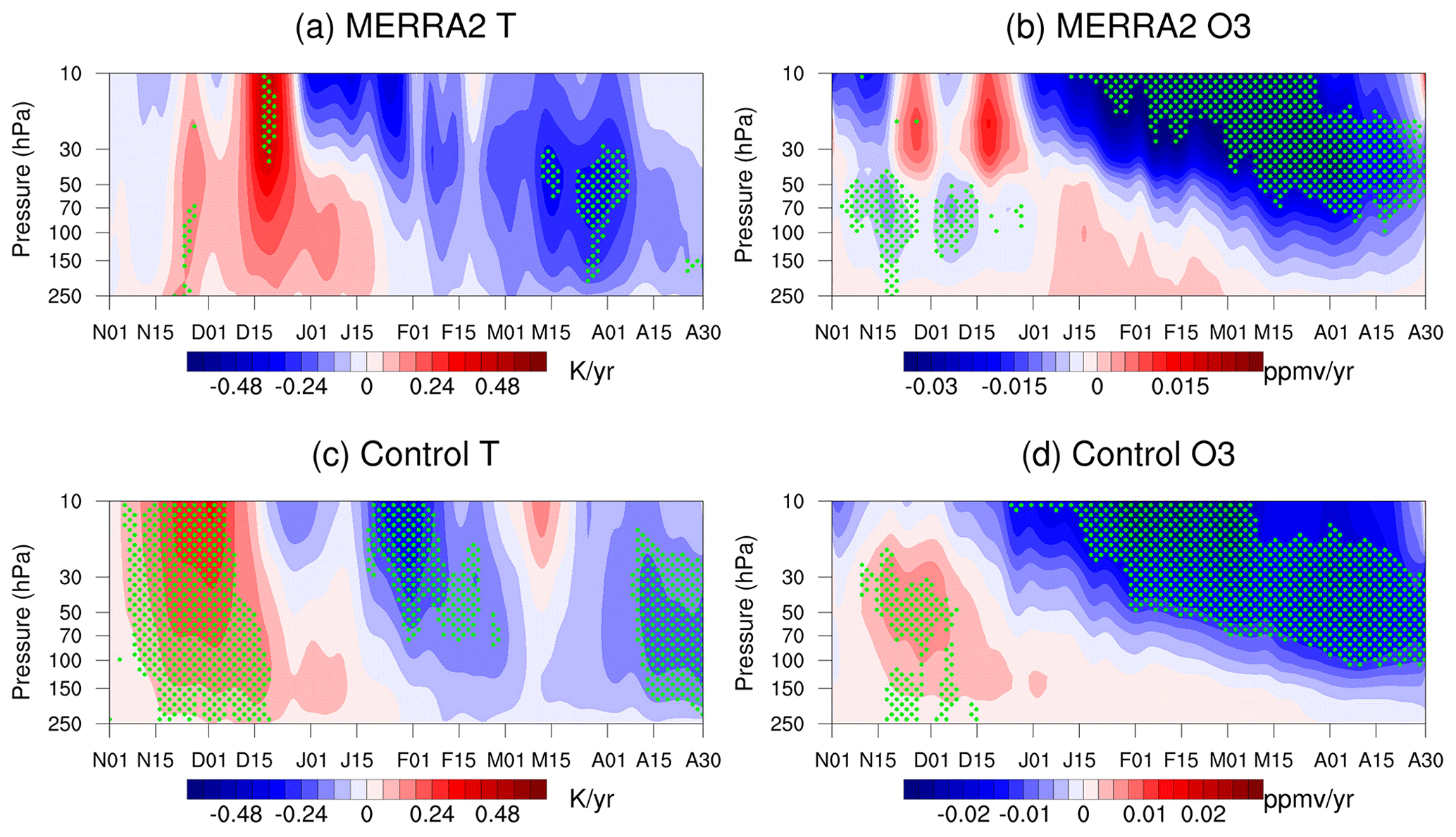
Figure 3 Time evolution of trends in daily (a, c) temperature and (b, d) ozone between 10 and 250 hPa in the polar cap regions (65–90° N) during winter and spring derived from MERRA2 and the ensemble mean of control experiments during the period 1980–2000. The green dotted regions indicate that the trends are statistically significant at the 90 % confidence level according to Student's t test.

Figure 4a, b shows the daily trends in temperature and ozone between 10 and 250 hPa in the polar regions (65–90° N) before 2000, derived from the ensemble O3clm experiments (for the simulation set-up, see Methods). The ensemble mean of O3clm experiments shows an insignificant temperature positive trend from November–December and a slightly unremarkable negative trend after December. This result is somewhat similar to that of the ensemble control experiments, but relatively weaker and not significant (Fig. 3c). The stratospheric ozone exhibits marginally positive trends between 30 and 250 hPa in November and December, and shows a significant negative trend between 10 and 70 hPa after December, which is weaker than that in the ensemble control experiments. Given that the ensemble O3clm experiments exclude the radiative and dynamic feedback of long-term ozone changes, the stratospheric ozone decline in late winter and spring essentially reflects the ozone depletion induced by increasing ODSs in the pre-2000 period (Fig. 4b). And the temperature cooling in late winter and spring (Fig. 4a) in the ensemble O3clm experiments may be related to stratospheric cooling induced by GHG (Tett et al., 1996; Hu and Guan, 2022). Figure 4c, d shows the differences in temperature and ozone trends before 2000 between the ensemble mean of the control experiments and O3clm experiments. Note that there are significant positive anomalies in temperature and ozone trends during November and early December, and significant negative anomalies after December, which are due to net ozone chemical–radiative–dynamical feedback effects (Fig. 4c, d). These significant differences suggest that ozone–climate interactions are crucial for long-term changes in AST and ozone.

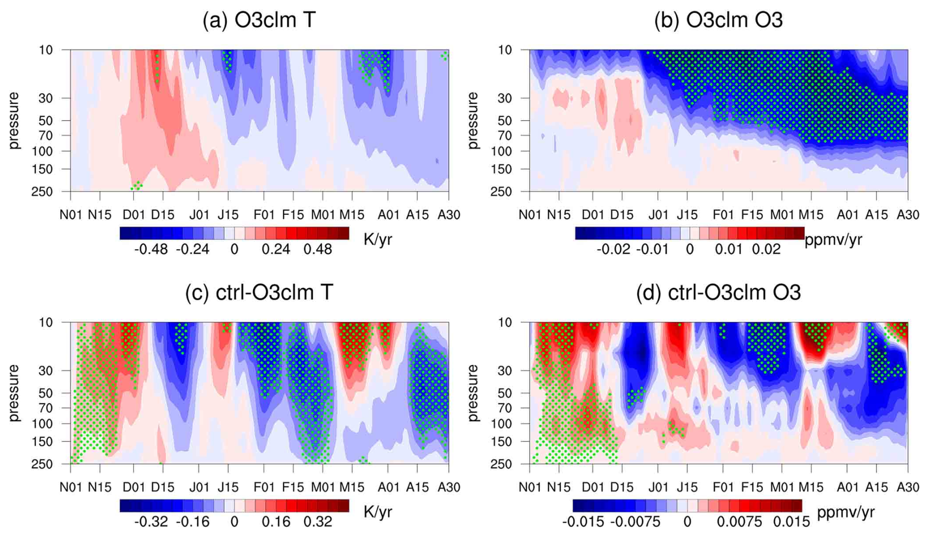
Figure 4 Time evolution of the trend of daily temperature and ozone over the levels between 10 and 250 hPa in the polar cap regions (65–90° N) during winter and spring derived from (a–b) the ensemble mean of the O3clm experiments and (c–d) the difference between the ensemble control experiments and ensemble O3clm experiments during the period 1980–2000. The green dotted regions indicate that the trends are statistically significant at the 90 % confidence level according to Student's t test.

4 The factors responsible for the trends in temperature from winter to spring

Ozone–climate interactions modulate stratospheric temperature through both radiative and dynamical pathways. Figure 5 shows the evolution of the shortwave heating rate (referred to as QRS) and longwave heating rate (referred to as QRL) trends from November to April, illustrating how ozone changes drive thermal responses that are further coupled to stratospheric dynamics. Figure 5 shows that both the ensemble control and O3clm experiments exhibit weak QRS trends from November to mid-February because sunlight cannot reach the Arctic regions. In the ensemble mean of the control experiments, QRL heating from November to early December shows a negative trend corresponding to the longwave cooling effect (Seppälä et al., 2025). In contrast, in the ensemble O3clm experiments, the ozone–climate interactions are removed and there are weaker QRL trends, which may be solely contributed by GHGs. QRL cooling in the ensemble control experiments occurs because a warmer air parcel, corresponding to the positive temperature trend in early winter, emits more longwave radiation. Note that this radiative effect is secondary and is overwhelmingly dominated by dynamical warming. The mechanisms behind these dominant dynamical processes are discussed in the following analysis (Figs. 6, 8).

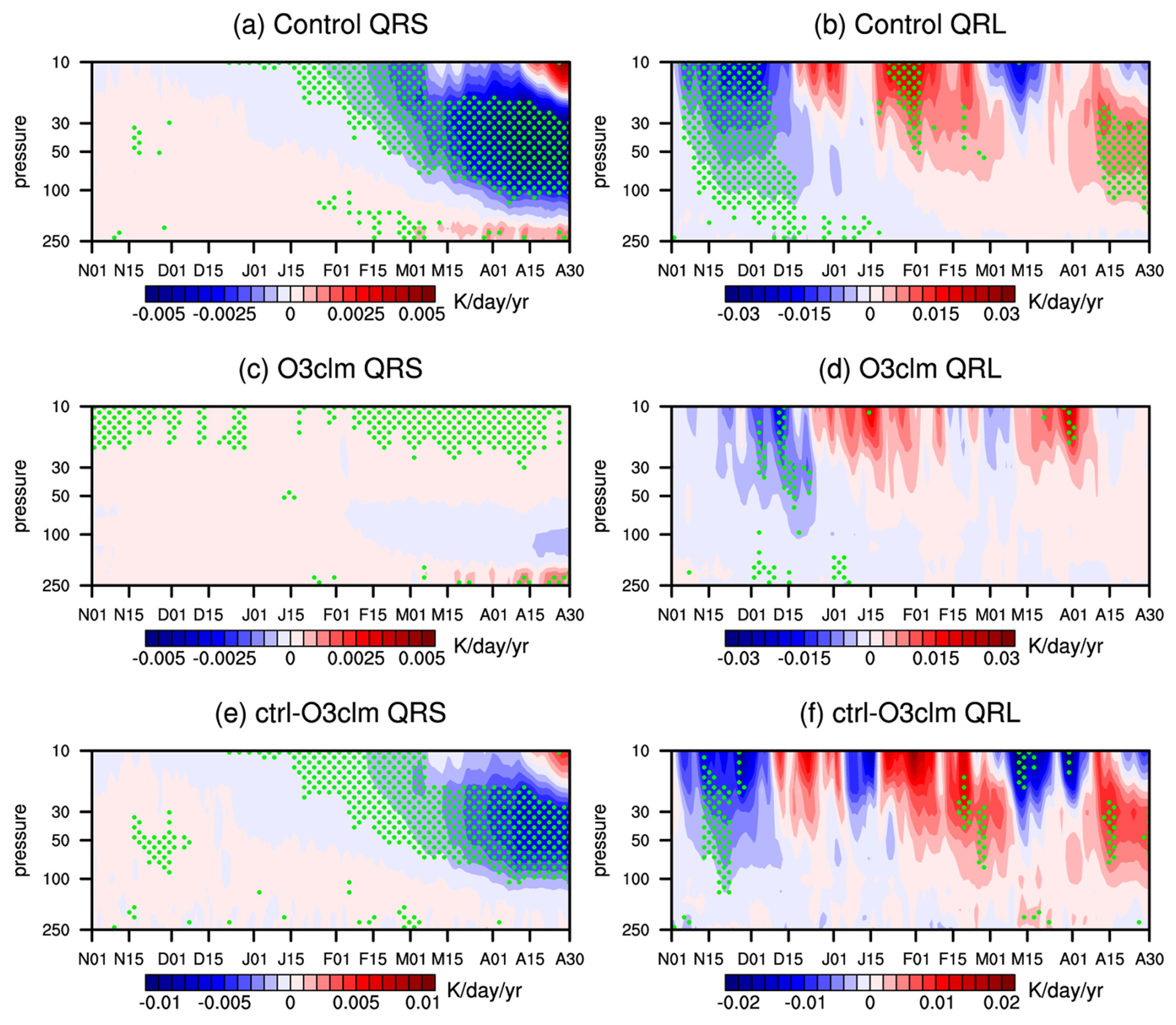
Figure 5 Time evolution of trends in the daily QRS and QRL between 10 and 250 hPa in the polar regions (65–90° N) during winter and spring derived from (a, b) the ensemble control experiments, (c, d) ensemble O3clm experiments and (e, f) the difference between ensemble control experiments and ensemble O3clm experiments during the period 1980–2000. The green dotted regions indicate that the trends are statistically significant at the 90 % confidence level according to Student's t test.

After February, the contribution of shortwave radiative processes to stratospheric temperature increases as sunlight reaches the Arctic region. The ensemble control experiments demonstrate that QRS shows a significant negative trend during the ozone-depletion period, which leads to a negative trend in temperature since 1980 (Figs. 2, 3). However, in the ensemble O3clm experiments, the radiative effects of ozone–climate interactions are inactivated, leading to insignificant changes in QRS throughout the entire winter and spring. In addition, negative temperature anomalies (Figs. 2c and 3a, c) correspond to the colder air parcel emitting less longwave radiation and thereby a positive QRL trend in spring. In the difference between the ensemble control experiments and O3clm experiments, QRS and QRL exhibit similar patterns to those in the ensemble control experiments.

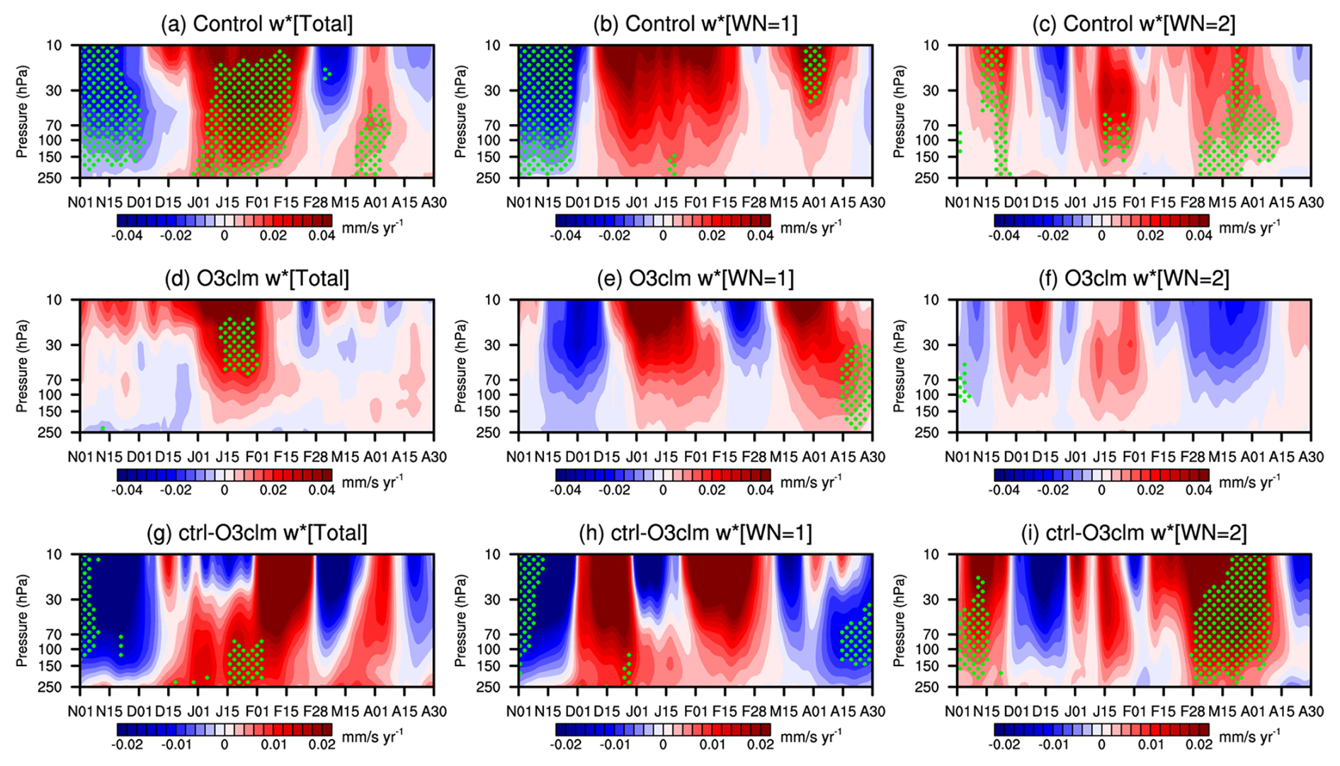
Figure 6 Linear trend of (a, d, g) the vertical component of the BDC (${\stackrel{\mathrm{‾}}{w}}^{*})$ and its contribution from (b, e, h) the wavenumber 1 and (c, f, i) wavenumber 2 components before 2000 between 10 and 250 hPa averaged in the polar regions (65–90° N) during winter and spring, derived from (a, b, c) the ensemble control experiments, (d, e, f) ensemble O3clm experiments and (g, h, i) the difference between the ensemble control experiments and ensemble O3clm experiments during the period 1980–2000. The green stippled regions indicate the trends of the BDC are significant at the 90 % confidence level according to Student's t test (the daily data are first processed with a 30 d low-pass filter to remove high-frequency signals).

The core process of ozone–climate interactions is ozone–circulation feedback. Figure 6 displays the trend in the downwelling branch of the BDC (${\stackrel{\mathrm{‾}}{w}}^{*})$ averaged over the polar regions (65–90° N) during the pre-2000 period in both the ensemble control experiments and O3clm experiments. We also decomposed these trends into contributions from wave 1 (Fig. 6b, e and h) and wave 2 (Fig. 6c, f and i). The ensemble mean of control experiments shows significant negative trends in ${\stackrel{\mathrm{‾}}{w}}^{*}$ from November to early December, corresponding to enhanced downwelling compared to the climatological mean, and positive trends in ${\stackrel{\mathrm{‾}}{w}}^{*}$ from late December to January, corresponding to weakened downwelling (Fig. 6a). In late February and early March, the ${\stackrel{\mathrm{‾}}{w}}^{*}$ trend in the upper stratosphere becomes negative (Fig. 6a). The linear trends in ${\stackrel{\mathrm{‾}}{w}}^{*}$ are basically the opposite of those of temperatures derived from the ensemble control experiments (Fig. 3c). This occurs because stronger (weaker) downwelling promotes enhanced (reduced) adiabatic polar warming relative to normal conditions. In addition, the ${\stackrel{\mathrm{‾}}{w}}^{*}$ trend contributed by wave 1 is similar to the total trend, suggesting that wave 1 dominates the trends in ${\stackrel{\mathrm{‾}}{w}}^{*}$. In the ensemble O3clm experiments, there is no negative trend in ${\stackrel{\mathrm{‾}}{w}}^{*}$ in November and early December (Fig. 6d–f). This result indicates that ozone–circulation feedback strengthens the downwelling in early winter, leading to stronger adiabatic warming; conversely, there are weakened downward motions that induce less adiabatic warming (an unusual cooling anomaly) from January to February, which is consistent with the reversal of the temperature trend at the end of December (Figs. 3, 4). The difference between the ensemble mean of the control experiments and O3clm experiments suggests a similar pattern to that of the ensemble control experiments (Fig. 6g, h and i). Overall, the changes in ${\stackrel{\mathrm{‾}}{w}}^{*}$ during early winter, particularly in November, are mainly modulated by ozone–climate interactions and adiabatic warming due to the strengthening of ${\stackrel{\mathrm{‾}}{w}}^{*}$, which play a crucial role in AST from November to early December. Similar results have been reported in previous studies (Albers and Nathan, 2013; Hu et al., 2019b). This dynamical heating dominates the longwave radiative cooling effect due to ozone–climate interaction, resulting in a warming of the middle and lower Arctic stratosphere during early winter.

Furthermore, the enhanced BDC may have an effect on the ozone concentration. The increase in stratospheric ozone during November–December and decrease during January–February (Fig. 4d) is partially caused by dynamical transport due to ozone–circulation feedback. We focus on the role of BDC in driving the ozone increase in early winter and its decrease in mid-winter, investigating the reasons for the reversal. Figure 7 shows the trend in stratospheric ozone budget from November to February between 10 and 250 hPa in the polar regions (65–90° N) in the pre-2000 period, which is decomposed into BDC and eddy transport of ozone (calculated by Eq. 8). In the ensemble control experiments, from November to December (early winter), the total ozone budget shows a significantly positive trend, indicating an increase in ozone concentrations. This trend is primarily driven by the sum of BDC and eddy transport. In mid-winter, the trend in ozone budget weakens and becomes negative, indicating a leveling off of increased ozone concentration. In contrast, in the ensemble O3clm experiments, the trend in the ozone budget is different from those in the ensemble control experiments and is not statistically significant from November to February. This demonstrates that, during early winter, the accelerated BDC intensifies poleward ozone advection by directly transporting ozone-rich air masses from tropical reservoirs to the polar region, and enhances downward transport of ozone from the upper stratosphere to the lower stratosphere. The ozone transport due to ozone–circulation feedback is reconfirmed by the difference between the ensemble mean of the control and O3clm experiments. At the end of December, the difference between the two experiments shows an intra-seasonal reverse in ozone transport, indicating that the ozone–circulation interactions can also give feedback to ozone concentrations.

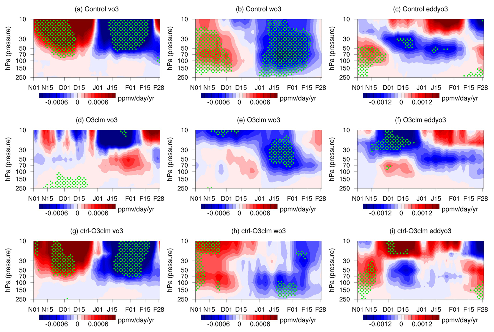
Figure 7 Dynamically produced ozone concentration trend, decomposed into (a, d, g) meridional and (b, e, h) vertical BDC transport and (c, f, i) eddy transport between 10–150 hPa in the polar regions (65–90° N) from November to February, derived from (a–c) the ensemble control, (d–f) the O3clm experiments and (g–i) the difference between the ensemble control experiments and ensemble O3clm experiments during the period 1980–2000. The trends over the dotted regions are statistically significant at the 90 % confidence level according to the Student's t test (the daily data are first processed with a 30 d low-pass filter to remove high-frequency signals). It is noted that the x axes denote the period from 1 November to 28 February.

In addition, ozone–climate interactions influence the AST by modulating planetary waves and the background conditions that govern wave propagation. Figure 8 shows the trends in stratospheric planetary wave activity over the subpolar regions (50–80° N) from November to April. In the ensemble control experiments, there is a significantly positive trend in the waves entering the stratosphere in November and early December before 2000, which is accompanied by intensified wave flux convergence in the middle stratosphere (approximately 10–50 hPa; Fig. 8a). However, in late December and January, the waves entering the stratosphere decrease, accompanied by weakened wave flux convergence. These features imply that stratospheric planetary wave activity is strengthened in November and early December and weakened in late December and January during the pre-2000 period. In contrast, in the ensemble O3clm experiments, waves entering the stratosphere in November and early December decrease, and there is no significant convergence trend before 2000 (Fig. 8d). The trends in the planetary wave are mainly contributed by the wave 1 component rather than by wave 2 (Fig. 8b, c, h and i). In November and early December, more propagation of planetary waves into the stratosphere weakens the circumpolar westerlies and increases the temperature in the Arctic lower stratosphere, which is consistent with the enhanced downward motions shown in Fig. 6g. The trends in planetary wave activity and E–P flux convergence in January and February are opposite to those in early winter. Overall, the changes in upward wave propagation and BDC make a major contribution to reverse the stratospheric temperature trend at the intra-seasonal time scale during winter. Note that the planetary wave activity only changes noticeably before February in the ensemble mean of control experiments and O3clm experiments, and then gradually weakens in spring. This suggests that dynamic feedback processes induced by ozone–climate interactions play a dominant role in winter.

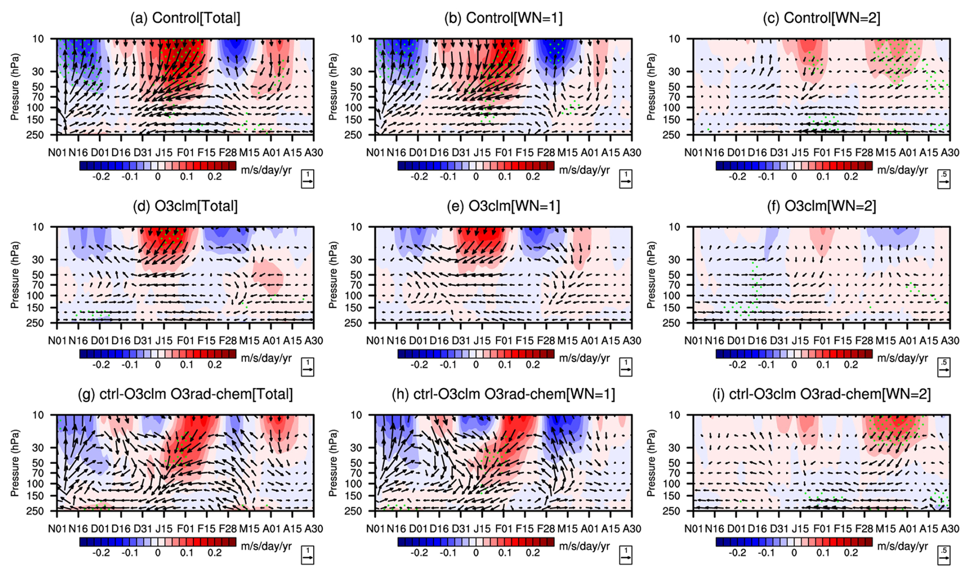
Figure 8 Trends in E–P flux (a, d, g; arrows; units of horizontal and vertical components are 10⁴ and 10² kg s⁻² yr⁻¹, respectively; an arrow pointing to the right indicates poleward propagation, whereas an arrow pointing to the left indicates equatorward propagation) and its divergence (shading) with their (b, e, h) wave 1 components and (c, f, i) wave 2 components over the levels between 10 and 250 hPa before 2000 averaged in the subpolar regions (50–80° N) during winter and spring, as derived from (a–c) the ensemble control experiments, (d–f) ensemble O3clm experiments and (g–i) the difference between the ensemble control experiments and ensemble O3clm experiments. The green stippled regions indicate the trends of the E–P flux divergence are significant at the 90 % confidence level according to Student's t test (the daily data are first processed with a 30 d low-pass filter to remove high-frequency signals).

The planetary waves entering the stratosphere are primarily modulated by propagating conditions in the upper troposphere and lower stratosphere regions (Albers and Nathan, 2013; Hu et al., 2019b, 2022). The refractive index (RI) is a good metric for assessing the atmospheric state for planetary wave propagation. According to the equation for RI (Eqs. S1, S2 in the Supplement), the change in the zonally averaged potential vorticity gradient (${\stackrel{\mathrm{‾}}{q}}_{\mathit{\phi }}$) is the main driving factor for the change in RI (Simpson et al., 2009; Zhang et al., 2020). In the ensemble control experiments, significant positive trends in RI persist during November in the middle and lower stratosphere (black line in Fig. S1a), implying that more planetary waves could enter the stratosphere due to ozone–climate interactions in early winter. This corresponds to the strengthened F_z (purple line in Figs. S1a, 8a). Note that the positive trends in ${\stackrel{\mathrm{‾}}{q}}_{\mathit{\phi }}$ and RI lead the increasing F_z by approximately one week. However, after mid-December, the RI trends become negative in the middle and lower stratosphere, suppressing upward wave propagation, which is consistent with reduced E–P flux during this period (Figs. 8a, S1a). There is a remarkable reversal of ${\stackrel{\mathrm{‾}}{q}}_{\mathit{\phi }}$ as a precursor. The reversal of ${\stackrel{\mathrm{‾}}{q}}_{\mathit{\phi }}$ is primarily driven by changes in the zonal wind vertical shear term (U_zz term; not shown). The negative ${\stackrel{\mathrm{‾}}{q}}_{\mathit{\phi }}$ trend persists until February in the middle and lower stratosphere, which basically corresponds to a negative trend in RI, which consequently affects the intra-seasonal reversal signal in the E–P flux (Figs. 8a, S1a). However, in the ensemble O3clm experiments, for most of winter, the RI and F_z show insignificant negative trends, which are markedly different from those derived from the ensemble control experiments. Nathan and Cordero (2007) pointed out that wave-induced ozone heating decrease wave drag by approximately 25 % in the lower stratosphere, favoring planetary wave propagation at this altitude during early winter in the present study (Fig. 8a, g). In the ensemble control experiments, the positive zonal wind vertical shear anomalies (not shown) at middle-latitudes in November increase ${\stackrel{\mathrm{‾}}{q}}_{\mathit{\phi }}$, which in turn raises the RI and enhances F_z, thereby weakening the polar vortex, and decelerating the circumpolar westerlies from December to January (the red line in Fig. S1). The decreased zonal wind at 60° N further suppresses the vertical propagation of planetary wave in the subsequent winter months, corresponding to the intra-seasonal reversal of F_z before and after December. Then, the weakening of F_z in the ensemble control experiments allows for a stronger recovery of the polar vortex due to wave-flow interaction in February. These features are absent in the ensemble O3clm experiments. It is indicated that the ozone–climate interaction plays a key role in regulating the stratospheric temperature and the changes of wave propagation by regulating ${\stackrel{\mathrm{‾}}{q}}_{\mathit{\phi }}$ and RI.

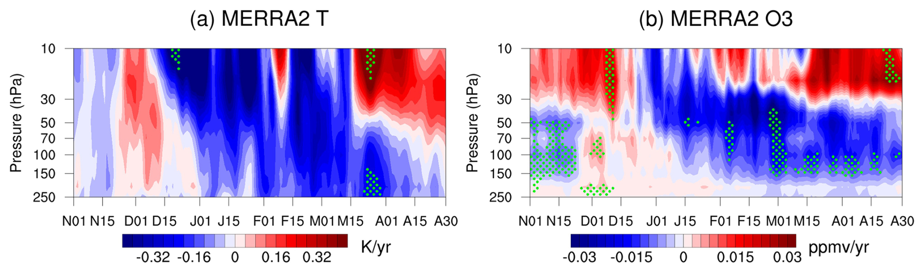
Figure 9 Time evolution of trends in daily (a) temperature and (b) ozone over the levels between 10 and 250 hPa in the polar regions (65–90° N) during winter and spring derived from MERRA2 after 2000. The green dotted regions denote that the trends are statistically significant at the 90 % confidence level according to Student's t test.

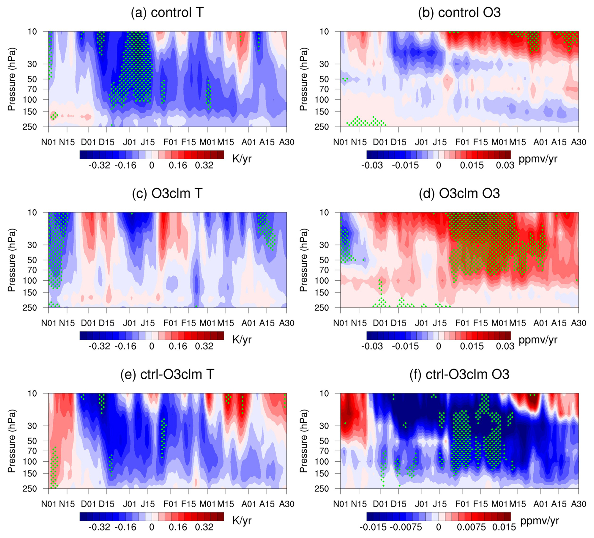
Figure 10 Time evolution of the trends in daily (a, c, e) temperature and (b, d, f) ozone over the levels between 10 and 250 hPa in the polar regions (65–90° N) during winter and spring derived from (a, b) the ensemble control experiments, (c, d) the ensemble O3clm experiments and (e, f) the difference between the ensemble control experiments and ensemble O3clm experiments during the period 2000–2020. The green dotted regions indicate that the trends are statistically significant at the 90 % confidence level according to Student's t test.

In the previous sections, we revealed the effect of ozone–climate interactions on stratospheric temperature and circulation during the ozone-depletion period before 2000. To understand how ozone–climate interactions work after 2000, Fig. 9 further illustrates the trend in the daily variation in temperature and ozone between 10 and 250 hPa in the polar regions (65–90° N) in the post-2000 period, on the basis of MERRA2 data. The results show an unremarkable decrease in temperature and ozone trends between 10 and 150 hPa during November. However, in December, there is a significant increasing trend in ozone across all levels and a slightly positive trend in temperature (Fig. 9a, b). From February to March, the temperature and ozone in the regions of the middle and lower stratosphere show significant negative trends. These changes are similar to those before 2000, with the difference being that the reversal of the negative trend occurs earlier. Compared with the pre-2000 period, there are positive anomalies for temperature and ozone in the middle and upper stratosphere in April after 2000, indicating that the post-2000 period experienced stratospheric ozone recovery (WMO, 2022).

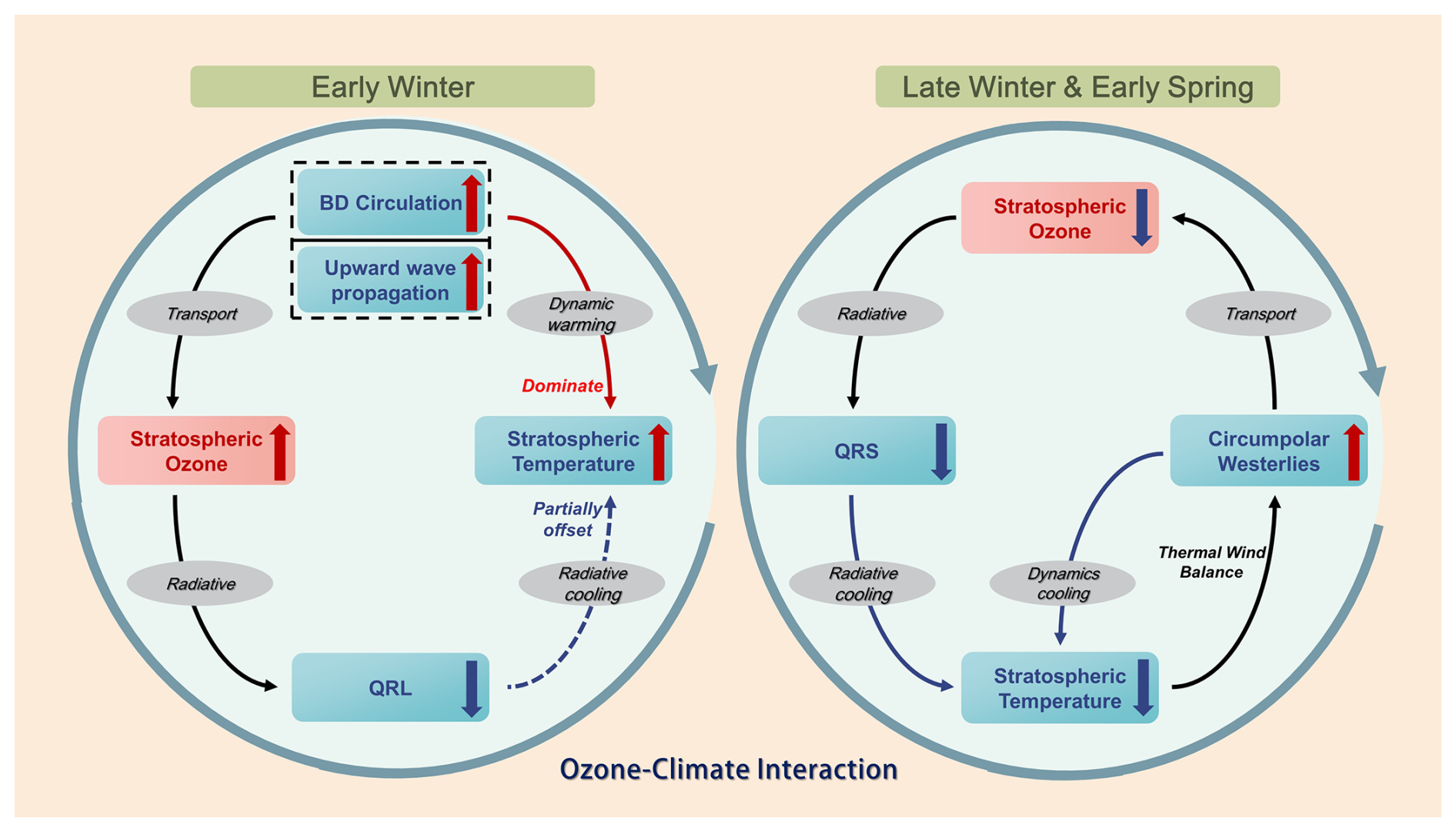
Figure 11 Schematic diagram of the ozone–climate interactions in the Arctic stratosphere during winter and spring. The red upward arrow indicates an increase, while the blue downward arrow denotes a decrease.

Figure 10 shows the results derived from the ensemble control experiments and ensemble O3clm experiments, and the difference between the ensemble mean of the two experiments. The ensemble mean of control experiments shows an insignificant positive temperature in the lower stratosphere during November and December and negative temperature trends during January and February, which are similar to the MERRA2 results. In the ensemble O3clm experiments, the temperature and ozone trends show totally different patterns from those in the observation and ensemble control experiments. Furthermore, in the post-2000 period, the stratospheric ozone shows significant positive trends in the O3clm experiments, which are not seen in the observation and control experiments. This is because the negative ozone trends in March and April induced by ozone–climate interactions may delay ozone recovery during spring through the shortwave radiative cooling effect. Also note that the differences in temperature and ozone between the ensemble mean of the control experiments and O3clm experiments (Fig. 10e, f) look somewhat like the pre-2000 results (Fig. 4c, d), but the differences are not significant most of the time. This suggests that the ozone–climate interactions continue to work after 2000, leading to intra-seasonal reversal trends in stratospheric temperature and ozone. However, this phenomenon may require examination over longer time scales, for example after significant ozone recovery has been observed in the Arctic, before a more detailed discussion of the mechanisms can take place.

5 Conclusion and discussion

This study investigates the effects of ozone–climate interactions on the temperature trends in the Arctic stratosphere during winter and early spring, using reanalysis datasets and CESM model simulations. We found that AST in early winter, particularly in November, significantly increases before 2000 (Figs. 2, 3 and 4), which is primarily driven by enhanced planetary wave propagation into the stratosphere and a strengthened BDC. The enhanced BDC also increases the stratospheric ozone during early winter. Notably, the ozone–circulation feedback of ozone–climate interactions plays a key role in modulating this temperature trend. Specifically, in early winter, ozone–circulation feedback can create an atmospheric state favorable for upward wave propagation, which is induced by the increases of ${\stackrel{\mathrm{‾}}{q}}_{\mathit{\phi }}$ in mid-latitude, and E–P flux convergence (Figs. 8, S1), which could lead to a strengthened BDC (Fig. 6) and thereby a positive trend in temperature and ozone (Figs. 3, 7) during early winter. These trends in BDC and planetary wave activity are predominantly driven by planetary wavenumber 1 (Figs. 6, 8). The wave-induced ozone heating increases lower-stratospheric wave propagation (Figs. 8, S1), and subsequently weakens the polar vortex during mid-winter (Fig. S1). Then, the upward propagation of planetary waves is suppressed, and consequently, the ASTs show opposite trends in January and February to early winter. During early spring, when solar radiation reaches the polar regions, reduction in ozone shortwave heating during the ozone-depletion period results in negative temperature trends during spring (Fig. 5). After 2000, the stratospheric temperature response to ozone changes is weaker than that before 2000 (Figs. 9, 10). Our results demonstrate that the ozone–climate interactions mainly influence stratospheric temperature trends through dynamic heating overwhelming radiative longwave cooling during early winter. In contrast, the trends in temperature during late winter and spring are primarily due to dynamic cooling and shortwave cooling. An integrated picture depicting the mechanisms in different seasons before 2000 is shown in Fig. 11.

The ozone–climate interactions are crucial processes in modulating the aforementioned AST trends. Similar to earlier findings, our study highlights the role of planetary wave activity and BDC in influencing AST. The present study provides more detailed information on the ozone–circulation feedback processes driven by ozone–climate interactions. The ozone–circulation feedback of interest consists primarily of the interactions between ozone changes, wave propagation and BDC, which regulate the dynamics of the Arctic stratosphere. Ozone-induced changes in wave propagation could modulate the vertical motions in the Arctic lower stratosphere, leading to changes in stratospheric temperature and circulation. The ozone transport associated with circulation changes could produce a feedback effect on polar ozone redistribution. Thus, it is plausible that the trends in stratospheric temperature and ozone are caused by an amplification of ozone–climate interactions. These ozone–climate interactions resemble previous findings on the climatic effects induced by zonally asymmetric ozone variations (McCormack et al., 2011; Rae et al., 2019; Zhang et al., 2020). Their experiments, that account for the phase overlap between zonally asymmetric ozone heating and planetary wave centers, tend to produce a climatologically warmer, weaker and more disturbed winter Arctic vortex compared to simulations driven solely by zonal-mean ozone forcing.

Notably, various factors may influence ozone–climate interactions. These factors include changes in GHG concentrations, nitrous oxide, volcanic activity or other atmospheric constituents that influence radiative and chemical processes in the stratosphere (Klobas et al., 2017; Meul et al., 2016; Ravishankara et al., 2009; Revell et al., 2015; Solomon et al., 2009). This raises questions about other potential feedback mechanisms for ozone–climate interactions in the future. Future studies are needed to better understand how and to what extent these factors can influence ozone–climate interactions. In addition, we acknowledge several limitations in our study. Methodologically, reliance on only one climate model simulation introduces inherent uncertainties due to climatic internal variability. A more complete solution to these limitations may require us to conduct longer historical simulation experiments to reduce experimental uncertainties using various chemistry-climate models. In summary, this study contributes to a better understanding of effects of ozone–climate interactions on the long-term temperature trend in the Arctic stratosphere, offering valuable insights for the development of climate models. Chemistry-climate models with ozone–climate interactions could make better predictions of stratospheric temperature changes, informing strategies for ozone protection and climate change mitigation.