Global ionospheric sporadic E intensity prediction from GNSS RO using a novel stacking machine learning method incorporated with physical observations

Sporadic E (E_s) layers, the irregularities of enhanced electron density commonly occurring in the ionospheric E region, are affected by the interactions between distinct atmospheric layers. E_s intensity (EsI) is a crucial parameter to describe E_s layer characteristics, while there still lacks the method for high-precision EsI prediction due to its complex spatiotemporal variation and physical driving mechanisms. We propose a novel stacking machine learning (SML) method for global EsI prediction, which combines the advantages from different ML models to obtain better performance than using a single ML model. Various E_s-related physical observations, including vertical ion convergence, gravity wave potential energy, and solar and geomagnetic indices, are incorporated as the inputs of SML together with the EsI derived from global navigation satellite system (GNSS) radio occultation (RO) measurements. SML performs well in both long-term and short-term EsI prediction and characteristics reconstruction. SML-predicted EsI is in good agreement with GNSS RO-derived EsI, with the mean error (ME) of 0.032 TECU km⁻¹ and root mean square error (RMSE) of 0.158 TECU km⁻¹. Taking ionosonde observations as reference, SML has the RMSE of 1.064 MHz, which is reduced by 20.1 %–40.5 % compared to existing prediction methods. The higher accuracy of our method than methods not incorporating physical observations illustrates the significance of considering multiple related physical factors when constructing the E_s prediction model. The proposed method can be expected to provide valuable information for not only ionospheric irregularities monitoring and space weather forecasting but also the mechanisms of E_s layer formation and atmospheric coupling.

1 Introduction

Ionospheric sporadic E (E_s) layers are thin-layer structures with abnormally sharp enhanced densities of electrons and metal ions, occurring frequently in the ionospheric E region with a major altitude range of 90–130 km. Existing studies show that the occurrence of E_s layers is driven by various physical mechanisms in the lower atmosphere, mesosphere–lower thermosphere (MLT), ionosphere, and space environment, such as the neutral wind shear (Chu et al., 2014), upward propagating gravity waves (GWs) (Qiu et al., 2023), atmospheric tides (Tang et al., 2022a), electric fields (Resende et al., 2016, 2021), solar activity (Yu et al., 2021), and geomagnetic field (Luo et al., 2021a; Moro et al., 2022), resulting in its highly uncertain and irregular spatial and temporal characteristics. Specifically, the neutral wind shear theory is widely accepted for the E_s layer formation in mid-latitudes, and the low-latitude E_s layers are well related to wind shear and equatorial electrojet plasma irregularities (Forbes, 1981; Raghavarao et al., 2002; Resende et al., 2013). In comparison, the particle precipitation during geomagnetic activity and the upward propagation of gravity waves are more efficient in concentrating the ions of E_s layers in high latitudes (Batista and Abdu, 1977; Kirkwood and Nilsson, 2000; MacDougall et al., 2000a, b). E_s layers may cause scintillations on the propagations of radio signals and severely affect the radio communication and satellite navigation. Therefore, the high-precision modeling and prediction of E_s layers not only is crucial for ionospheric irregularities monitoring and space weather forecasting but also provides solutions for understanding the mechanisms of E_s layer formation and coupling of distinct atmospheric layers, while it still remains a challenging task due to its complex patterns and influencing factors.

Traditionally, E_s layers are detected by ground-based devices such as ionosonde and incoherent scatter radar (Leighton et al., 1962; Mathews, 1998; Heinselman et al., 1998). With the development of the global navigation satellite system (GNSS) over the past 2 decades, the space-borne GNSS radio occultation (RO) missions have been widely applied to investigate the climatology of E_s occurrence rates and E_s intensity (EsI) in recent years (Arras et al., 2008; Chu et al., 2014; Yu et al., 2019; Xu et al., 2022; Liu et al., 2024a). Most RO missions consist of one or several low-earth-orbit (LEO) satellites, which can acquire all-weather and wide-area ionospheric observations with high vertical resolution. Based on the large number of accumulated RO data, some empirical models were established using statistical methods to describe the global EsI distribution (Hu et al., 2022; Yu et al., 2022; Niu and Fang, 2023). However, because of the high uncertainty and irregularity of EsI, these empirical models are difficult to predict the localized and short-term E_s variations. Besides, these numerically established models are not incorporated with physical observations such as wind shears, GWs, and solar flux and geomagnetic indices and thus cannot estimate EsI based on the E_s-related physical mechanisms. To overcome this limitation, some scholars compared the morphologies of RO-derived EsI and physical data to analyze their relationships (Qiu et al., 2019; Yu et al., 2019; Yamazaki et al., 2022), but these analyses were only qualitative and did not quantitatively reveal their correlations.

Recently, advances in artificial intelligence algorithms have provided new perspectives for data analysis in geosciences and many other fields. Machine learning (ML) is a powerful tool fitting complex nonlinear relationships between multiple variables, which has been employed to resolve the regression and classification problems in geoscience and is proven to have better performance compared with traditional methods. Currently, there are few studies on EsI prediction based on ML methods. Although Emmons et al. (2023) and Tian et al. (2023) used ML models for the detection and reconstruction of E_s layers, there were few data on E_s-related physical mechanisms used for model training in their studies. The incorporation of data about the background neutral wind, GWs, and solar and geomagnetic activity should contribute to better performance of E_s layer reconstruction and prediction. In addition, although a large number of ML models have been utilized in ionospheric predictions, the performance of single models is limited by their respective shortcomings. For example, a neural network (NN) performs well in learning complex patterns from large quantities of available data but often tends to easily overfit in the analysis of limited datasets (Hinton et al., 2012). Besides, due to the “black box” nature of a NN, it is difficult to investigate potential relationships between inputs and inner structure of NNs, so NN outputs are often lacking of interpretability (Hastie et al., 2009). Comparatively, the bagging and boosting ML models like random forest (RF) and gradient boosting decision tree (GBDT) tend to show better performance and interpretability than NN on some small datasets (Zhukov et al., 2021; Han et al., 2022). To bridge this gap, the stacking machine learning (SML) method is implemented to obtain better accuracy and generalization than a single model. SML uses the stacking strategy (Wolpert, 1992), which combines several base models and incorporates their outputs into a meta model, to leverage the efficiency of different models together; thus the possible errors of a single model can be complemented by other models. Compared with other ensemble methods like bagging and boosting, it has a better ability to reduce both variance and bias. SML has been successfully applied to solve some ionospheric predictive problems. For example, Asamoah et al. (2024) proposed a stacked model combining three ML models to predict total electron content (TEC) over a single station and demonstrated its better performance than the single models. Liu et al. (2024b) utilized a hybrid ensemble model to forecast ionospheric irregularities over the Brazilian sector. However, to our knowledge, the SML method has not been applied for EsI prediction till now.

Hence, in this article, we present an SML model for global ionospheric EsI prediction, where a variety of observations representing E_s-related physical mechanisms are used as inputs of our model, including the vertical ion convergence (VIC) driven by neutral wind shear, the GW activity, and the solar and geomagnetic indices. They are incorporated together with EsI derived from GNSS RO measurements into the proposed SML model. The SML method selects five widely adopted ML models, RF, light gradient boosting machine (LightGBM), eXtreme Gradient Boosting (XGBoost), support vector machine (SVM), and back propagation neural network (BPNN) as the base models, and a multilayer perceptron neural network (MLPNN) is utilized as the meta model, i.e., the second part of the SML model to optimally integrate the predictions generated by base models and generate the final prediction. The prediction performance of SML is validated using RO-derived EsI and ionosonde data under different space weather conditions and is also compared with other prediction methods.

2 Data and materials

2.1 GNSS RO-derived EsI

Constellation Observing System for the Meteorology, Ionosphere, and Climate (COSMIC) is a global RO mission launched in April 2006, with the goal of providing GNSS RO data for operational weather prediction, climate analysis, and space weather forecasting (Syndergaard et al., 2006). COSMIC consists of six LEO satellites with an orbital altitude of 800 km and inclination of 72° and provides more than 2000 globally distributed TEC profiles per day during its full operation stage. COSMIC TEC profiles are the profiles of the calibrated TEC below COSMIC LEO satellite altitude, and they have a high vertical resolution of better than 2 km and thus are suitable for the detection of E_s layers, which are with small vertical scales. In this study, COSMIC TEC profiles during 2006–2019 are collected as the data source for deriving EsI. Since the altitude range of E_s layers considered in this paper is 90–130 km, a quality control process is taken at first to remove the profiles with negative TEC values and the bottom heights higher than 90 km, and 93.45 % of raw TEC profiles passed quality control and are retained for further analysis. Figure 1 shows the traces of qualified COSMIC TEC profiles on 1 August 2007. It indicates that COSMIC TEC data have a dense global coverage that is a great data source for global ionospheric investigations.

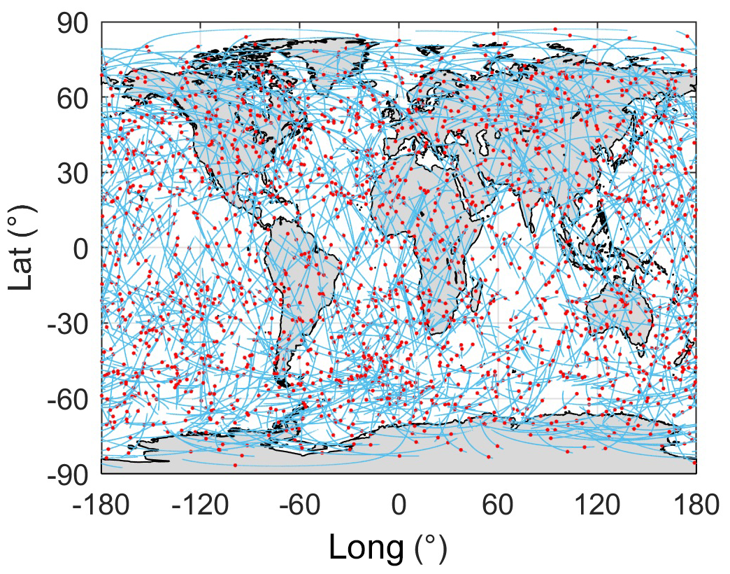
Figure 1 The traces of qualified COSMIC TEC profiles on 1 August 2007 (blue lines). The red points represent the locations corresponding to Smax.

We use a single spectrum analysis (SSA) method as described in Hu et al. (2022) to obtain the Smax index (unit: TECU km⁻¹), a proxy for EsI, from qualified TEC profiles. The TEC disturbances caused by E_s layers are extracted from original TEC profiles using SSA. Smax is defined as the maximum vertical gradient of TEC disturbances in the altitude range of 90–130 km, and the corresponding altitude is designated as the altitude of E_s layer. The reasonableness and effectiveness of Smax as the proxy of EsI have been verified by Niu et al. (2019) and Hu et al. (2022).

2.2 Ionosonde EsI

E_s critical frequency (foEs) is a conventional parameter characterizing EsI. Ionosondes provide reliable ground-based local foEs observations. In this study, foEs data downloaded from National Earth System Science Data Center of China (NESSDC) and UK Solar System Data Center (UKSSDC) are used to validate the prediction results of SML. The foEs observations at 1 h intervals, all manually scaled, are obtained from 15 ionosondes. Figure 2 shows the spatial distribution of ionosonde stations.

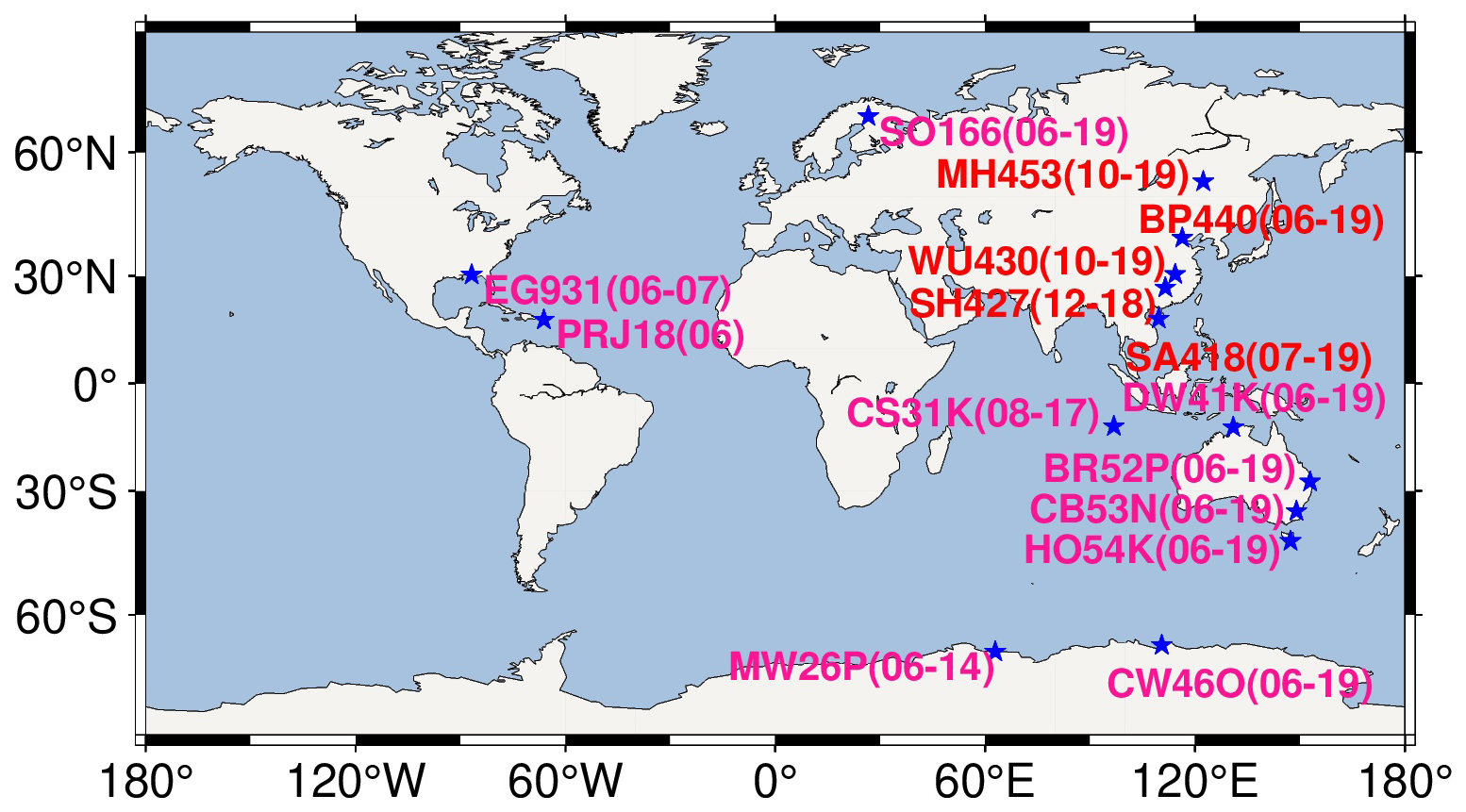
Figure 2 Spatial distribution of 15 ionosonde stations. The red and pink stations represent those from NESSDC and UKSSDC, respectively. In the brackets behind each station name, the corresponding time period of data is presented in the format of yy-yy.

2.3 VIC simulated by HWM14

The wind shear theory has been proven to be the most significant factor influencing the formation of mid-latitude E_s layers (Chu et al., 2014; Luo et al., 2021a). In the procedure of VIC driven by vertical wind shears in horizontal neutral winds, the metal ions are compressed into a thin layer by Lorentz force, and then the electrons drift along the magnetic field lines and converge to form an E_s layer (Mathews, 1998). We employ Horizontal Wind Model 2014 (HWM14) (Drob et al., 2015) to simulate VIC at the location of E_s layer. The vertical ion drift velocity w caused by the horizontal neutral wind shear can be written as follows:

$$\begin{array}{}\text{(1)}& w={\displaystyle \frac{r\cos I}{\mathrm{1}+r^{\mathrm{2}}}}U+{\displaystyle \frac{\cos I\sin I}{\mathrm{1}+r^{\mathrm{2}}}}V,\end{array}$$

where U and V are the zonal and meridional velocities of horizontal neutral wind, respectively, which are calculated by HWM14; I is the geomagnetic inclination angle; $r=v_i/w_i$, which is the ratio of the ion-neutral collision frequency to ion gyrofrequency (Nygrén et al., 2008); and $w_i=eB/M$, where e and M are the mass and charge of ion, respectively, and B is the magnetic field strength. Qiu et al. (2019) and Yu et al. (2019) indicated that E_s layers tend to appear in regions with negative vertical zonal wind shears ($\partial w/\partial z<\mathrm{0}$, where z is the altitude). Therefore, it is assumed that only positive values of VIC contribute to E_s layer formation:

$$\begin{array}{}\text{(2)}& \mathrm{VIC}=\left\{\begin{array}{c}-\frac{\partial w}{\partial z},-\frac{\partial w}{\partial z}>\mathrm{0}\\ \mathrm{0},-\frac{\partial w}{\partial z}\le \mathrm{0}.\end{array}\right.\end{array}$$

2.4 GW activity extracted from GNSS RO data

Recent studies have shown that the upward propagating GWs can transport energy and momentum from the lower atmosphere to the mesosphere and lower thermosphere, causing ionospheric disturbances and contributing to the formation of E_s layers (Qiu et al., 2023; Seid et al., 2023). COSMIC temperature profiles are able to cover a wide altitude range of 0–60 km with the vertical resolution better than 0.1 km, which are ideal data sources for studying GW activity. The proxy for GW activities, GW potential energy (E_p), can be calculated by the following equations:

$$\begin{array}{}\text{(3)}& {\displaystyle }{E}_{\mathrm{p}}={\displaystyle \frac{\mathrm{1}}{\mathrm{2}}}{\displaystyle \frac{g^{\mathrm{2}}}{N^{\mathrm{2}}}}{\left({\displaystyle \frac{T^{\prime }}{\stackrel{\mathrm{‾}}{T}}}\right)}^{\mathrm{2}}\text{(4)}& {\displaystyle }{N}^{\mathrm{2}}={\displaystyle \frac{g}{\stackrel{\mathrm{‾}}{T}}}\left({\displaystyle \frac{\partial \stackrel{\mathrm{‾}}{T}}{\partial z}}+{\displaystyle \frac{g}{c_p}}\right),\end{array}$$

where g is the gravitational acceleration, N is the buoyancy frequency, $\stackrel{\mathrm{‾}}{T}$ is the background temperature, $T^{\prime }=T-\stackrel{\mathrm{‾}}{T}$ is the temperature perturbation caused by GWs, and c_p=1004.5 J (kg K)⁻¹ is the isobaric heating capacity. To derive background temperature $\stackrel{\mathrm{‾}}{T}$ that represents longer waves like tides and planetary waves, global daily temperature profiles are binned into 10°×15° latitude–longitude grids with an altitude interval of 0.1 km to obtain daily mean temperature maps at each altitude level, and an S transform is applied on each zonal component of mean temperature maps to derive gridded data of $\stackrel{\mathrm{‾}}{T}$. The temperature perturbation T^′ is obtained by subtracting $\stackrel{\mathrm{‾}}{T}$ from original temperature profiles, and then GW E_p is calculated using Eqs. (3) and (4). The detailed procedure for extracting GW E_p is described in Luo et al. (2021b).

Figure 3 Variations of F10.7 and Dst indices during 2006–2019.

2.5 Solar and geomagnetic indices

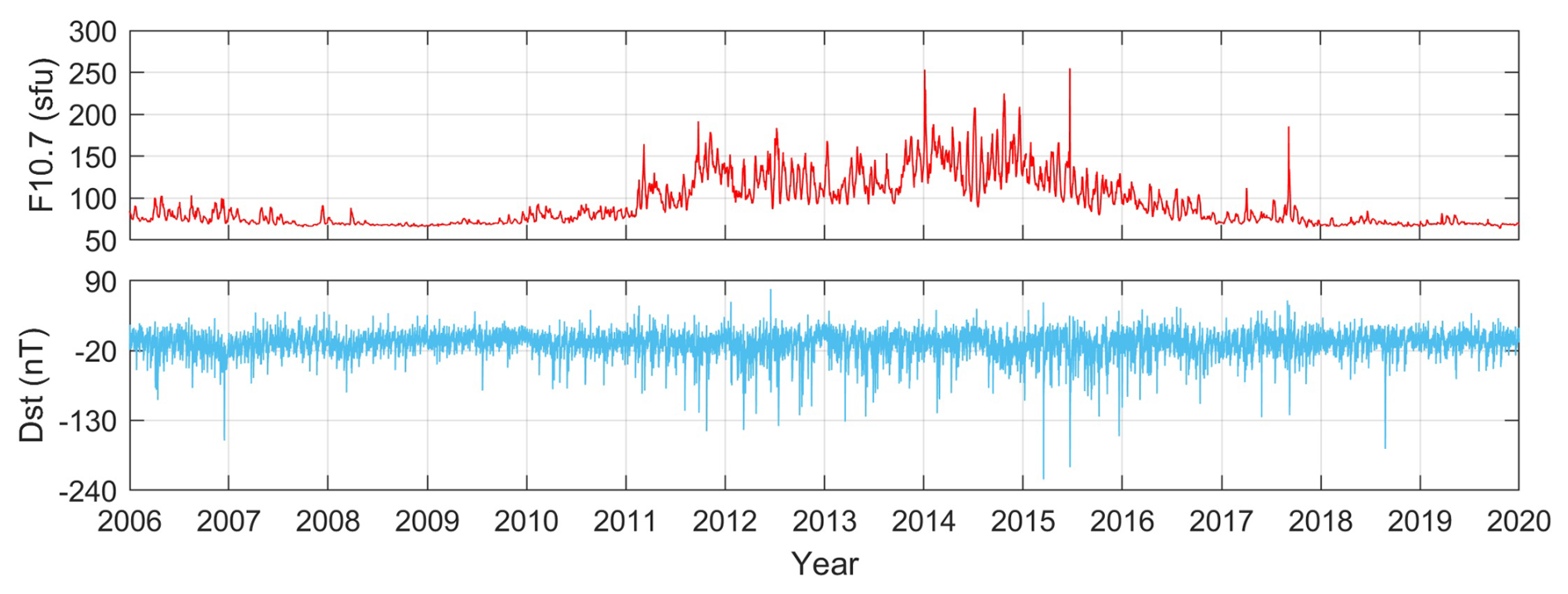
EsI is also affected by solar and geomagnetic conditions (Yu et al., 2021; Tang et al., 2022b). The solar radiation flux F10.7 and Dst indices are used to represent the solar and geomagnetic activity. We choose Dst index rather than 3 h Kp or Ap indices because Dst has a higher time resolution of 1 h. Figure 3 shows the variations of F10.7 and Dst indices during 2006–2019.

3 Methodology

3.1 Accuracy evaluation metrics

The mean error (ME), root mean square error (RMSE), and correlation coefficient (CC) are used as metrics to evaluate the accuracy of prediction results, which are calculated as

$$\begin{array}{}\text{(5)}& \left\{\begin{array}{l}\mathrm{ME}=\frac{\mathrm{1}}{n}\sum _{i=\mathrm{1}}^n\left(y_i-{\widehat{y}}_i\right)\\ \mathrm{RMSE}=\sqrt{\frac{\mathrm{1}}{n}\sum _{i=\mathrm{1}}^n{\left(y_i-{\widehat{y}}_i\right)}^{\mathrm{2}}}\\ \mathrm{CC}=\frac{\mathrm{cov}\left(y_i,{\widehat{y}}_i\right)}{{\mathit{\sigma }}_{y_i}\cdot {\mathit{\sigma }}_{{\widehat{y}}_i}},\end{array}\right.\end{array}$$

where n is the total number of prediction results; y_i and ${\widehat{y}}_i$ are the predicted and observed EsI, respectively; $\mathrm{cov}\left(y_i,{\widehat{y}}_i\right)$ is the covariance between y_i and ${\widehat{y}}_i$; and ${\mathit{\sigma }}_{y_i}$ and ${\mathit{\sigma }}_{{\widehat{y}}_i}$ are the standard deviations of y_i and ${\widehat{y}}_i$, respectively. The units of both ME and RMSE are TECU km⁻¹. CC has no unit.

3.2 Dataset configuration and segmentation

The proposed EsI prediction method aims to build a nonlinear functional model between the target (EsI) and inputs (spatiotemporal information and physical observations). Therefore, the time, latitude, longitude, and altitude corresponding to each RO-derived EsI (Smax), as well as the VIC, GW E_p, F10.7, and Dst, are formed into samples and fed into SML. To reduce the input feature complexity and modeling costs, the time of each sample is expressed as follows:

$$\begin{array}{}\text{(6)}& \mathrm{time}=\mathrm{year}+(\mathrm{DOY}+\mathrm{UT}/\mathrm{24})/\mathrm{365.25},\end{array}$$

where DOY and UT are day of year and universal time, respectively.

In SML method, the training and validation set is used for the training of the base models, and their prediction values become the training and validation set of the meta model. Since the cross-validation (CV) strategy is utilized for optimization of the SML model (see Sect. 3.3.2), samples of the entire dataset collected during 2006–2019 are divided into two groups: training and validation set (80 %, from 22 April 2006 to 31 December 2013) and testing set (20 %, from 1 January 2014 to 31 December 2019). Note that there are fewer samples after 2014 due to the decline in the number of measurements caused by the aging and loss of COSMIC satellites. Nevertheless, it in turn allows for a longer time period of the testing set and a more comprehensive evaluation of SML performance.

3.3 SML model development

3.3.1 ML models

SML combines the advantages from different ML models to obtain better performance than a single ML model. Diverse types of ML models should be selected to make SML fully incorporate their strengths, which require the selection of appropriate base models to simultaneously reduce the bias and variance. In this study, five ML models are utilized as base models, including RF, LightGBM, XGBoost, SVM, and BPNN. RF is a tree-based parallel ensemble ML algorithm using the bagging technique that is widely applied for classification and regression problems in GNSS and remote sensing tasks. RF is effective in reducing the variance of the model and has an improved robustness to outliers. Comparatively, LightGBM and XGBoost are sequential ensemble ML models based on the boosting technique. They use the gradient boosting technique with outstanding performance in reducing bias of numerous datasets. SVM is an ML method based on the principle of structural risk minimization. It utilizes the structural risk minimization theory to suppress the overfitting problem and minimize empirical risk and confidence interval. BPNN is a widely used NN model with high adaptability and learning ability for regression problems. It comprises three types of fully connected layers, i.e., the input layer, hidden layer(s), and output layer, which help to better capture complex nonlinear relationships.

Figure 4 The structures of RF, LightGBM, XGBoost, SVM, BPNN, and MLPNN.

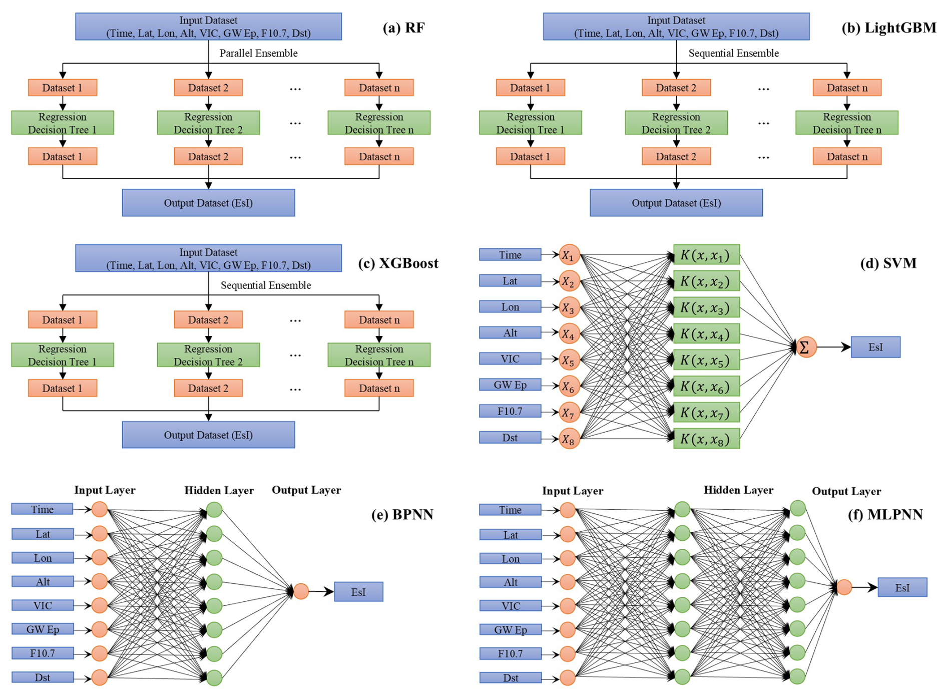
Furthermore, MLPNN is also a common NN model to solve regression problems. It has a similar structure with BPNN, while the main difference between MLPNN and BPNN lies in their activation functions. Here we use MLPNN as the meta model to find the optimal combination of base models, and the structures of the base models and meta model are shown in Fig. 4.

The mathematical expressions for all the ML models used are presented in Eqs. (7)–(12):

$$\begin{array}{}\text{(7)}& \mathrm{RF}\left(\mathit{x}\right)={\displaystyle \frac{\mathrm{1}}{M}}\sum _{m=\mathrm{1}}^M{T}_m\left(\mathit{x}\right),\end{array}$$

where x is the inputs, M is the number of trees, and T_m(x) is the mth tree output.

$$\begin{array}{}\text{(8)}& \mathrm{LightGBM}\left(\mathit{x}\right)={\displaystyle \frac{\mathrm{1}}{M}}\sum _{m=\mathrm{1}}^M{T}_m\left(\mathit{x}\right)W_m,\end{array}$$

where W_m is the weight of the mth tree. LightGBM is similar to GBDT, but compared with the depth-wise tree growth approach, it grows trees using the leaf-wise approach that focuses on nodes with the highest loss change, which is better at handling large datasets and improving prediction accuracy.

$$\begin{array}{}\text{(9)}& \mathrm{XGBoost}\left(\mathit{x}\right)={\displaystyle \frac{\mathrm{1}}{M}}\sum _{m=\mathrm{1}}^M{T}_m\left(\mathit{x}\right)W_m\end{array}$$

XGBoost is also similar to GBDT, while it offers a parallel tree boosting algorithm to improve computation efficiency. Actually, LightGBM and XGBoost are new optimized implementations for GBDT using different techniques.

$$\begin{array}{}\text{(10)}& \begin{array}{rl}& \mathrm{SVM}\left(\mathit{x}\right)=\mathit{w}\mathit{\phi }\left(\mathit{x}\right)+\mathit{b}\\ s.t.& min\left[{\displaystyle \frac{\mathrm{1}}{\mathrm{2}}}{∥\mathit{w}∥}^{\mathrm{2}}+C\sum _{i,j=\mathrm{1}}^L\left({\mathit{\xi }}_i,{\mathit{\xi }}_j\right)\right],\end{array}\end{array}$$

where w is the weight vector, φ is the nonlinear mapping function, b is the bias, L is the number of input samples, C is the penalty factor specifying the degree of penalty for outliers, and ξ_i and ξ_j are relaxation factors. Equation (9) can be solved by introducing Lagrange multipliers to obtain the regression function of SVM, in which φ is usually replaced by the radial basis function kernel $K(x_i,x_j)=\exp (-\mathit{\gamma }{∥x_i-x_j∥}^{\mathrm{2}})$, where γ is the kernel parameter. The details of SVM algorithm can be found in Yetilmezsoy (2019).

$$\begin{array}{}\text{(11)}& \begin{array}{rl}& {\mathrm{BPNN}}_k\left(\mathit{x}\right)=f\left(\sum _{j=\mathrm{1}}^L{w}_{kj}{x}_j+b_k\right)\\ & {\mathrm{MLPNN}}_k\left(\mathit{x}\right)=g\left(\sum _{j=\mathrm{1}}^L{w}_{kj}{x}_j+b_k\right),\end{array}\end{array}$$

where BPNN_k and MLPNN_k are the outputs of the kth neuron, and f(⋅) and g(⋅) are the activation functions of BPNN and MLPNN, respectively. We select the sigmoid and hyperbolic tangent functions as the activation functions of BPNN and MLPNN, respectively, which can be written as

$$\begin{array}{}\text{(12)}& \begin{array}{rl}& f\left(x\right)={\displaystyle \frac{\mathrm{1}}{\mathrm{1}+e^{-x}}}\\ & g\left(x\right)={\displaystyle \frac{\mathrm{2}}{\mathrm{1}+e^{-\mathrm{2}x}}}-\mathrm{1}.\end{array}\end{array}$$

3.3.2 Model optimization

Hyperparameters are the internal configuration parameters for ML models. The optimization of hyperparameters is important for improving the accuracy and generalizability of ML models. To determine the optimal hyperparameters while maintaining a relatively low computational cost, the grid search method is adopted to optimize the two hyperparameters with the greatest impact on the model. Specifically, for each model, a set of candidate values of the two hyperparameters to be optimized is defined in the parameter space, the model performance for each hyperparameter combination is evaluated, and the best-performing hyperparameter combination is defined as the optimal hyperparameter. During the grid search process, a 5-fold CV is utilized. The training and validation set is randomly divided into five non-overlapping folds. For each iteration of training and evaluation, the ith fold ($i=\mathrm{1},\mathrm{2},\mathrm{\dots },\mathrm{5}$) is used as the validation set, and the remaining folds are used as the training set. The average results of these iterations are denoted as the final performance evaluation.

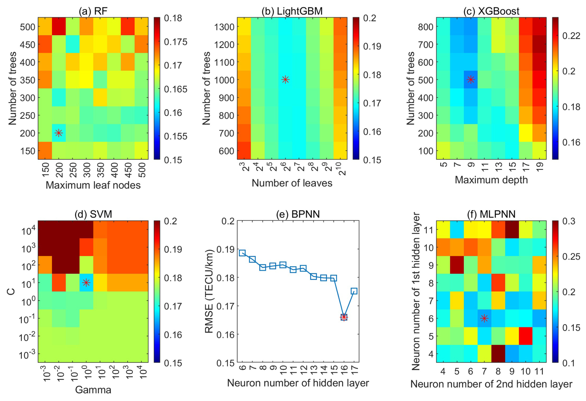
Figure 5 Grid search results (RMSE) for the optimization of RF, LightGBM, XGBoost, SVM, BPNN, and MLPNN. The red asterisks denote the optimal hyperparameter combination of each ML model.

Figure 5 shows the optimized hyperparameters, the candidate values, and the optimal values (denoted by red asterisks) of hyperparameters for each ML model. For RF (bagging model), the number of leaf nodes and the number of trees are selected as the hyperparameters to be optimized, and they are optimally determined as 200 and 200, respectively, while for LightGBM and XGBoost (boosting model), the number of leaves and the maximum depth play the more important roles in improving model performance, and they are optimally computed to 63 and 9, respectively. As shown in Eq. (9), the penalty factor C and the kernel parameter γ have significant impacts on the performance of SVM regressor. In this sense, they are selected for optimization with optimal values of 10 and 1, respectively. For BPNN and MLPNN, the number of hidden layer(s) and the neuron number in each hidden layer are key hyperparameters in determining the accuracy of the network. Since one hidden-layer-based NN can approximate the arbitrarily small error among most bounded continuous functions (Hornik et al., 1989), we only use one hidden layer in BPNN, while two hidden layers are adopted in MLPNN to better combine the predictions from base models. The optimal neuron number in the hidden layer(s) can be determined empirically based on the range from $\mathrm{2}\sqrt{n}+\mathit{\mu }$ to 2n+1, where n and μ are the neuron numbers in input and output layers, respectively. Therefore, the neuron numbers of BPNN and MLPNN are validated from 6 to 17 and from 4 to 11, respectively, and the optimal neuron numbers corresponding to the minimum RMSE are 16 for BPNN, and 6 and 7 for MLPNN, respectively. By optimizing these ML models, their performance, generalizability, and interpretability are improved so that they are more suitable for the specific task of EsI prediction in this study.

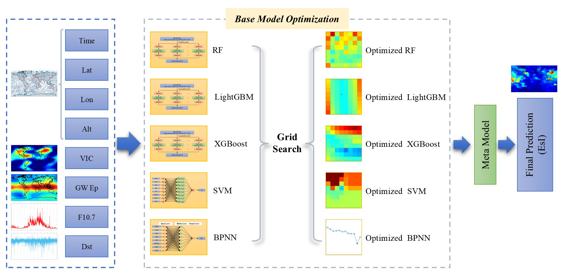
Figure 6 Framework of the SML model.

3.3.3 SML model architecture

In the training stage of the SML model, the outputs of RF, LightGBM, XGBoost, SVM, and BPNN on the training and validation set are fed into MLPNN as its input data, and its outputs are the final predicted EsI. This process is also similar in the test stage. The framework of SML is shown in Fig. 6.

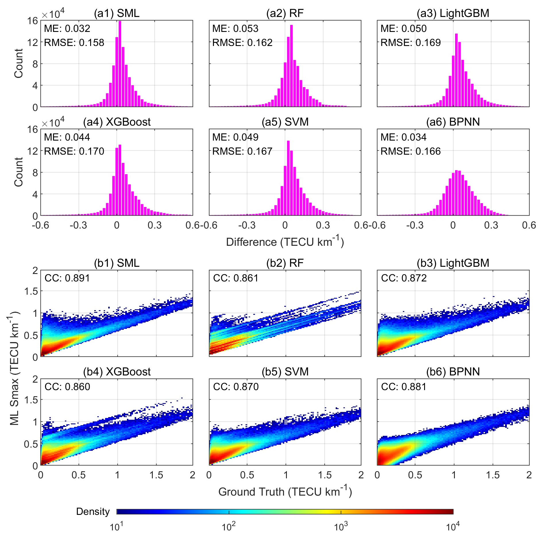
Figure 7 (a) Histograms and (b) density scatter plots of the comparisons of EsI predicted by SML and by base models with ground truth.

4 Results

4.1 Comparison of the SML model and base models

Both the SML model and the base models with the optimal hyperparameters are fitted on the training set. Then they are employed to make predictions on the testing set, and the prediction results are compared with the ground truth. Figure 7 illustrates the histograms and the density scatter plots of the comparisons of EsI predicted by SML and base models with ground truth. SML shows the much more aggregated histogram than the histograms of base models, which means that SML has the best agreement with ground truth among all ML models, with the minimum ME/RMSE of 0.032/0.158 TECU km⁻¹. Compared to the maximum ME and RMSE of 0.053 and 0.170 TECU km⁻¹ for the base models, SML has the improvement of 39.6 % and 7.1 %, respectively. The density scatter plots show that SML also has the highest CC of 0.891. As mentioned above, RF is more robust for outliers and more effective in reducing variances and thus has a lower RMSE than other base models. Comparatively, the other base models, especially BPNN, play an important role in reducing bias, and they outperform RF in terms of the overall prediction accuracy of EsI, as demonstrated by their MEs. By combining the strengths of different types of ML models, SML is able to achieve predictions with both lower biases and lower variances compared with all base models.

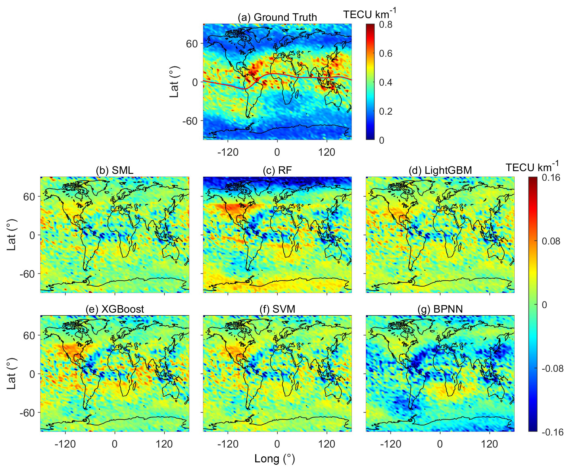
Figure 8 Latitude–longitude distribution of (a) ground truth and the difference between ground truth and the EsI predicted by (b) SML, (c) RF, (d) LightGBM, (e) XGBoost, (f) SVM, and (g) BPNN on the testing set. The red line denotes the geomagnetic equator.

In addition to the overall performance, the global distributions of EsI predicted by the models are also compared. Figure 8 presents the latitude–longitude maps of the differences between ground truth and the EsI predicted by SML and by base models on the testing set. Here the EsI maps represent the average EsI in the latitude–longitude bin of 2.5°×5° over the period of testing set. Specifically, RF has larger deviations than other models in North America (30–50° N and 80–120° W), in the South American Magnetic Anomaly (SAMA) zone (30–60° S and 20° W–40° E), and near the geomagnetic equator (denoted by the red line in Fig. 8a), which are the regions with smaller EsI due to the near horizontal geomagnetic field lines (Yu et al., 2019; Luo et al., 2021a). RF also has a considerable underestimation of EsI in the Arctic region. The other base models, especially BPNN, have overall smaller biases than RF, while they have more outliers exhibited as localized small patches with larger prediction errors at mid-latitudes and low latitudes. On the other hand, SML has the best prediction accuracies and the least number of outliers in the regions mentioned above, which is due to the SML avoiding the shortcomings of different base models by selectively integrating their outputs.

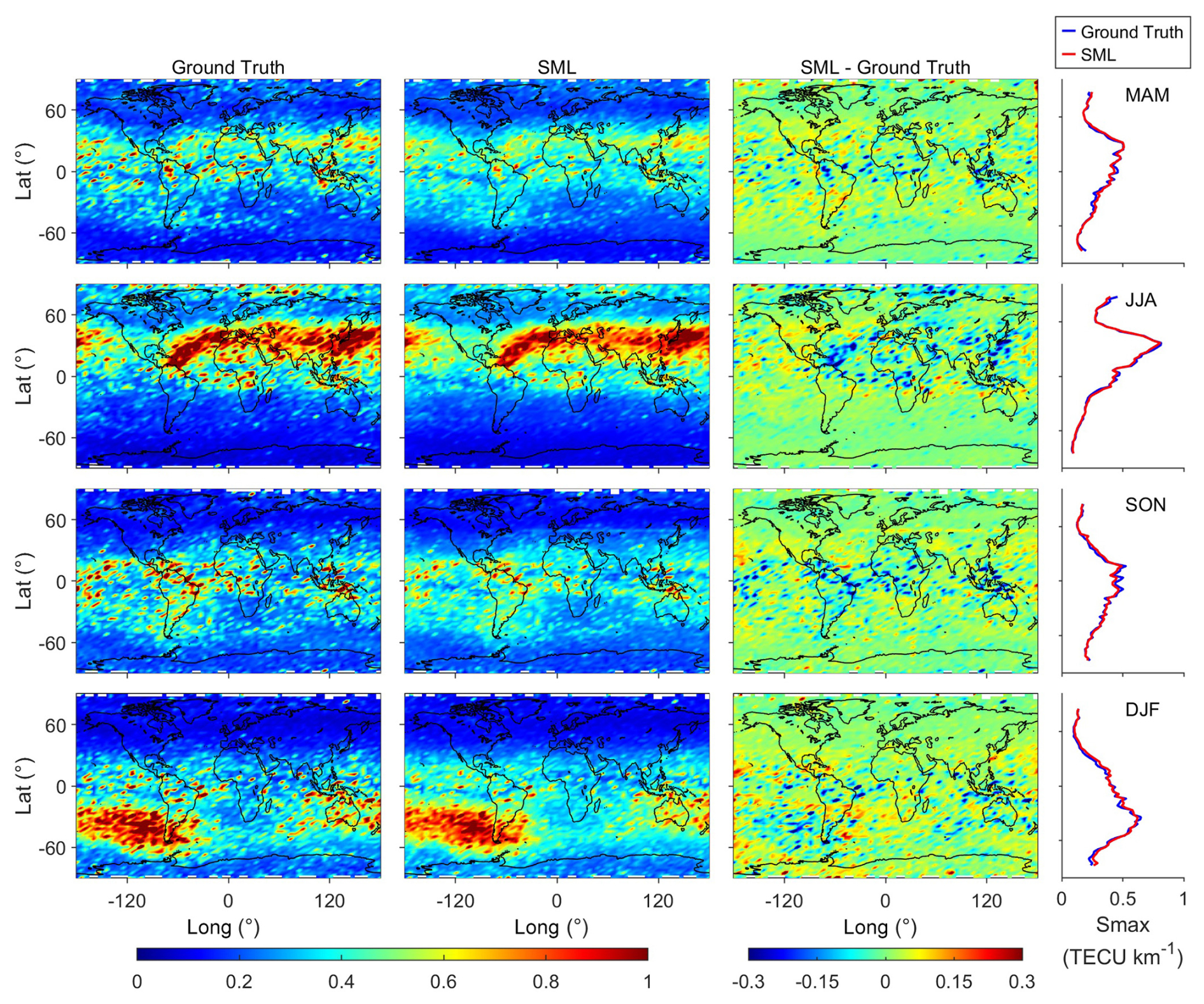
Figure 9 Latitude–longitude and latitudinal distributions of ground truth, SML-predicted EsI, and the corresponding error maps in four seasons.

Based on the above comparisons, SML has the highest CC and the smallest ME and RMSE, i.e., the best prediction performance. In the following sections, only the SML model is selected to assess the ability in reconstructing the complex long-term and short-term characteristics of EsI morphology, and we also compare the SML predictions with ionosonde observations for external validation of the prediction performance.

4.2 Long-term evaluation of SML performance

The long-term evaluation of SML prediction performance is conducted on the whole testing set, i.e., 2014–2019. Figure 9 presents the latitude–longitude and latitudinal distributions of ground truth, SML-predicted EsI, and the corresponding error maps in four seasons, which are categorized as MAM (March, April, and May), JJA (June, July, and August), SON (September, October, and November), and DJF (December, January, and February). Visual inspection shows that SML accurately simulates the seasonal variation of EsI. SML successfully shows the larger EsI that peaks in the banded area at mid-latitudes of the summer hemisphere and reaches the valley values in winter hemisphere, which is primarily dominated by the seasonal variation of meteor flux and the resulting metallic ion content, coupled with the neutral wind shear (Haldoupis et al., 2007). The weaker EsI in North America, in the SAMA zone, and along the geomagnetic equator due to the lower geomagnetic inclination angle is well reconstructed by SML predictions. Furthermore, the SML-predicted latitudinal distribution of EsI also agrees well with ground truth in all the four seasons. The larger EsI moves northward or southward with seasonal variations, which is under the control of wind shear at mid-latitudes. While at latitudes higher than 70°, there is also strong EsI which is larger than that at 60°, and this is no longer due to the wind shear but the vertical transport of ions and electrons caused by GWs propagating upward along near vertical geomagnetic field lines (Kirkwood and Nilsson, 2000). It indicates that the SML model can clearly reconstruct and predict the larger EsI in mid-latitudes and high latitudes dominated by different physical mechanisms and can comprehensively consider the impact of multiple influencing factors. The SML prediction errors are between ±0.1 TECU km⁻¹ in most areas, demonstrating the excellent prediction performance in long-term EsI prediction. The MEs of SML predictions for the four seasons are 0.004/−0.005/0.001/0.012 TECU km⁻¹, and RMSEs are 0.146/0.166/0.143/0.176 TECU km⁻¹, respectively. Nevertheless, we can see from the error maps that the areas of underestimation beyond ±0.1 TECU km⁻¹ are mainly concentrated at the peak of EsI in the summer hemisphere. The possible explanation for this phenomenon is that larger EsI is the minority of the training set (predominantly occurs in the summer hemisphere only), and the trained model fits this part of data slightly worse than smaller EsI. Improvement in the prediction performance for larger EsI should be required for future study.

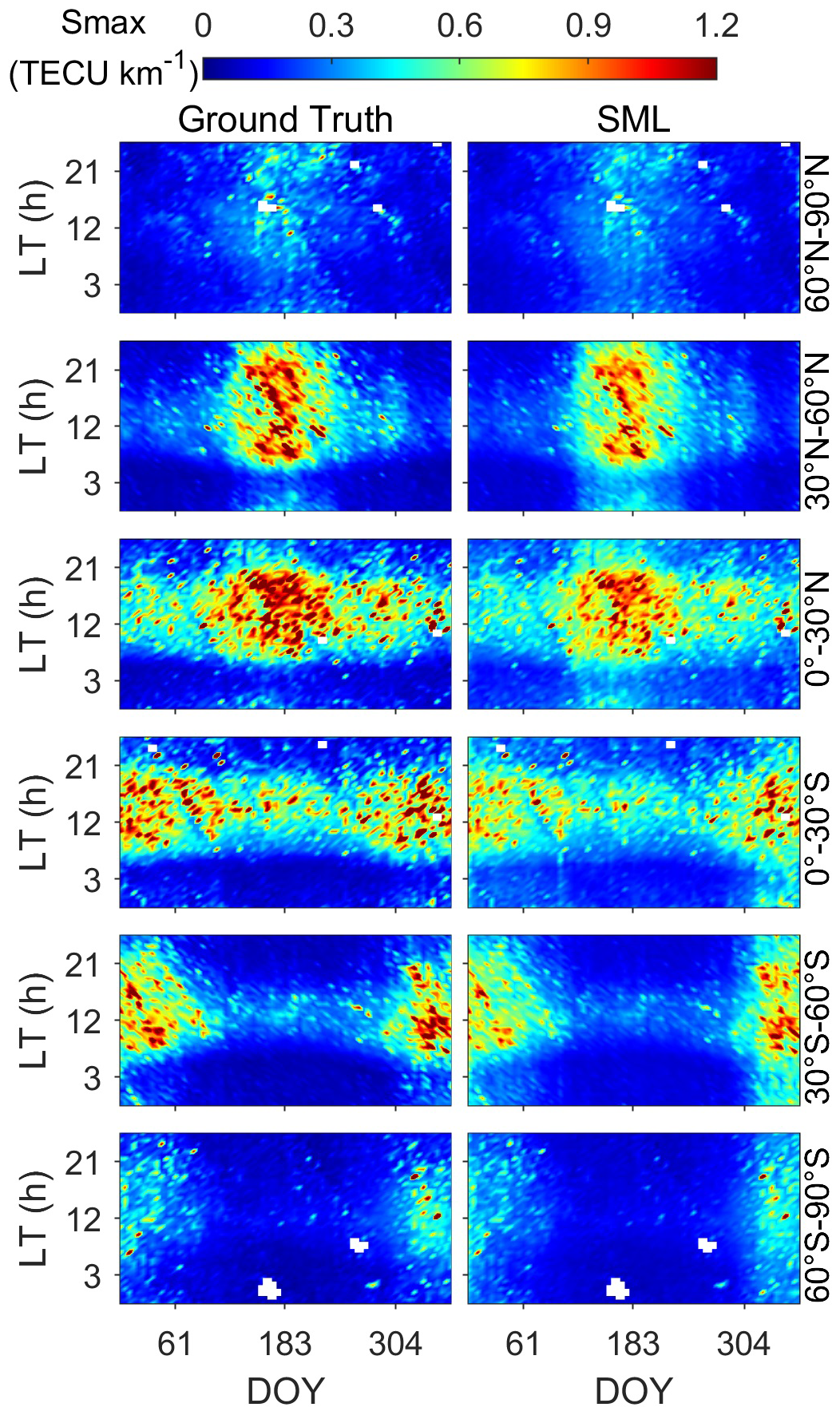
Figure 10 LT-DOY distributions of ground truth and SML-predicted EsI. The right label of the right panel of each row represents the latitude range of this row.

Figure 10 shows the local time day of year (LT-DOY) distributions of ground truth and SML-predicted EsI at different latitude ranges in 2014–2019. Larger EsI mainly exists in daytime, increasing after sunrise and decreasing after sunset. The EsI tidal signatures reconstructed by SML, mainly dominated by the wind shear and atmospheric tides (Yu et al., 2019), are consistent with ground truth, which can be identified on summer days with diurnal tides (starting around 10:00 LT) occurring at low latitudes (30° N–30° S) and semi-diurnal tides (starting around 08:00 and 16:00 LT) occurring at mid-latitudes (30–60° N and 30–60° S). Although the EsI seasonal variation in the Southern Hemisphere (SH) is opposite to that in the Northern Hemisphere (NH), the diurnal and semi-diurnal tides can still be discerned, only with a slightly lower peak intensity. Figure 10 indicates the effectiveness of SML in reconstructing tidal signatures of EsI.

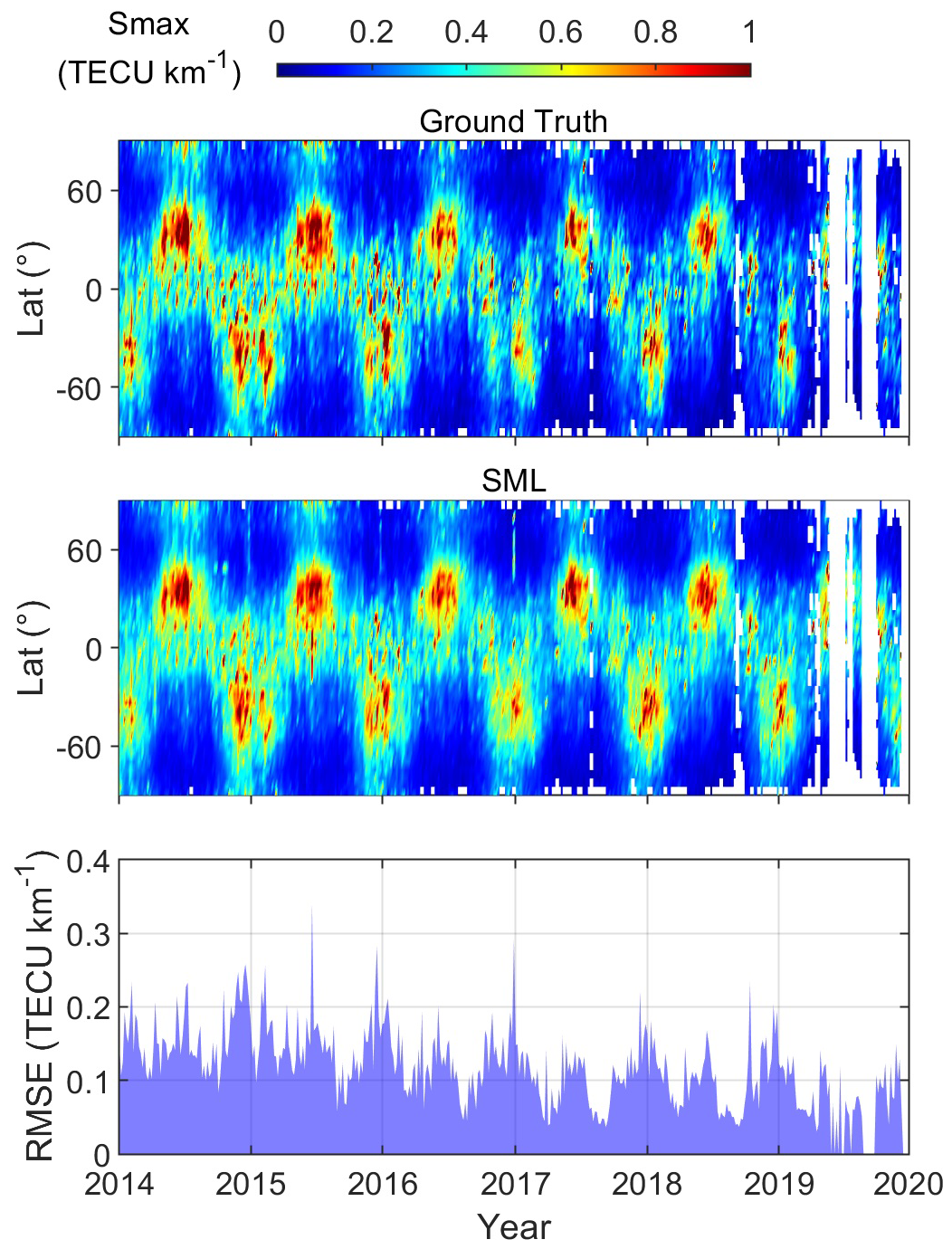
Figure 11 Latitudinal distribution of daily ground truth and SML-predicted EsI, as well as the daily RMSE on the testing set.

Figure 11 plots the latitudinal distribution of daily SML-predicted EsI and the daily RMSE on the whole testing set, with blank areas indicating the days without EsI data. The results show that the morphology characteristics of SML predictions are close to those of ground truth. SML succeeds in capturing the hemispheric asymmetry of EsI; i.e., EsI is generally slightly higher in the NH summer than in the SH summer of the same year, which is also found by Luo et al. (2021a) and Xu et al. (2022). This is mainly due to the lower EsI in the SAMA zone caused by the distribution of horizontal geomagnetic field, which diminishes the EsI over the corresponding latitude zones. Furthermore, the daily RMSE in Fig. 11 is generally stable below 0.2 TECU km⁻¹, with unusual sudden enhancements only in a few days. Overall, these results fully demonstrate the good ability of SML for stable EsI prediction and characteristics reconstruction in long-term periods.

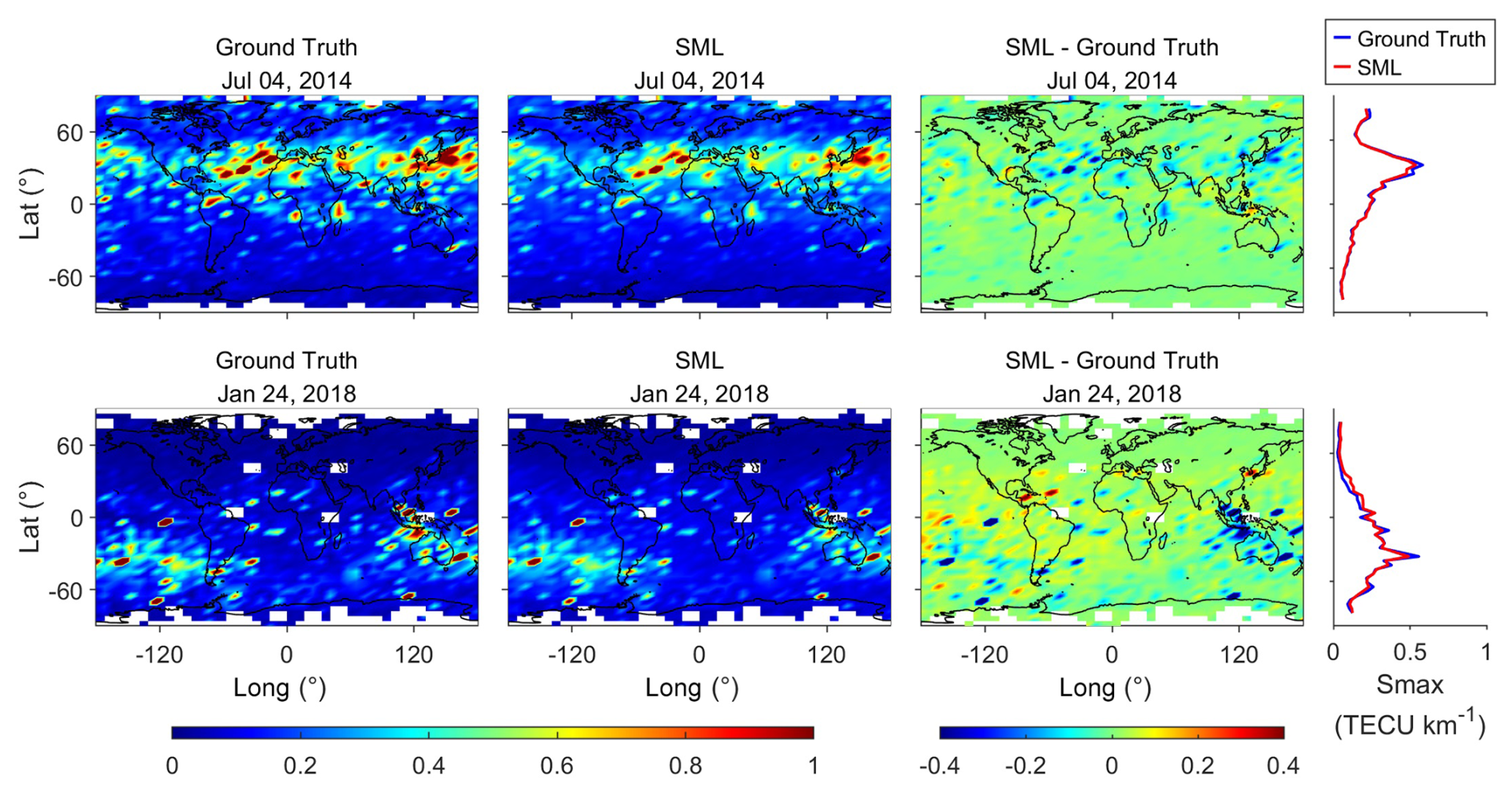
Figure 12 Latitude–longitude and latitudinal distributions of ground truth, SML-predicted EsI and the corresponding error maps during geomagnetic quiet times on 4 July 2014 and 24 January 2018.

4.3 Short-term evaluation of SML performance

The response of EsI to geomagnetic storms has been widely reported (Resende et al., 2021; Moro et al., 2022; Tang et al., 2022b; Qiu and Liu, 2025), which is usually a combined effect of neutral wind and electric field variations. We have conducted two case studies to evaluate the short-term prediction performance of SML during the geomagnetic quiet and storm time periods. Figure 12 shows the latitude–longitude and latitudinal distributions of ground truth, SML-predicted EsI, and the corresponding error maps on 2 quiet days, 4 July 2014 and 24 January 2018. Compared with ground truth, SML can effectively predict the general distribution of EsI, particularly the considerable agreement in latitudinal distribution, which is similar to that in Fig. 9. The prediction errors are mostly within ±0.1 TECU km⁻¹, with a small number of underestimates which are with larger errors mainly existing in the summer hemisphere. The ME/RMSE for the 2 quiet days are −0.006/0.183 and 0.006/0.133 TECU km⁻¹, respectively.

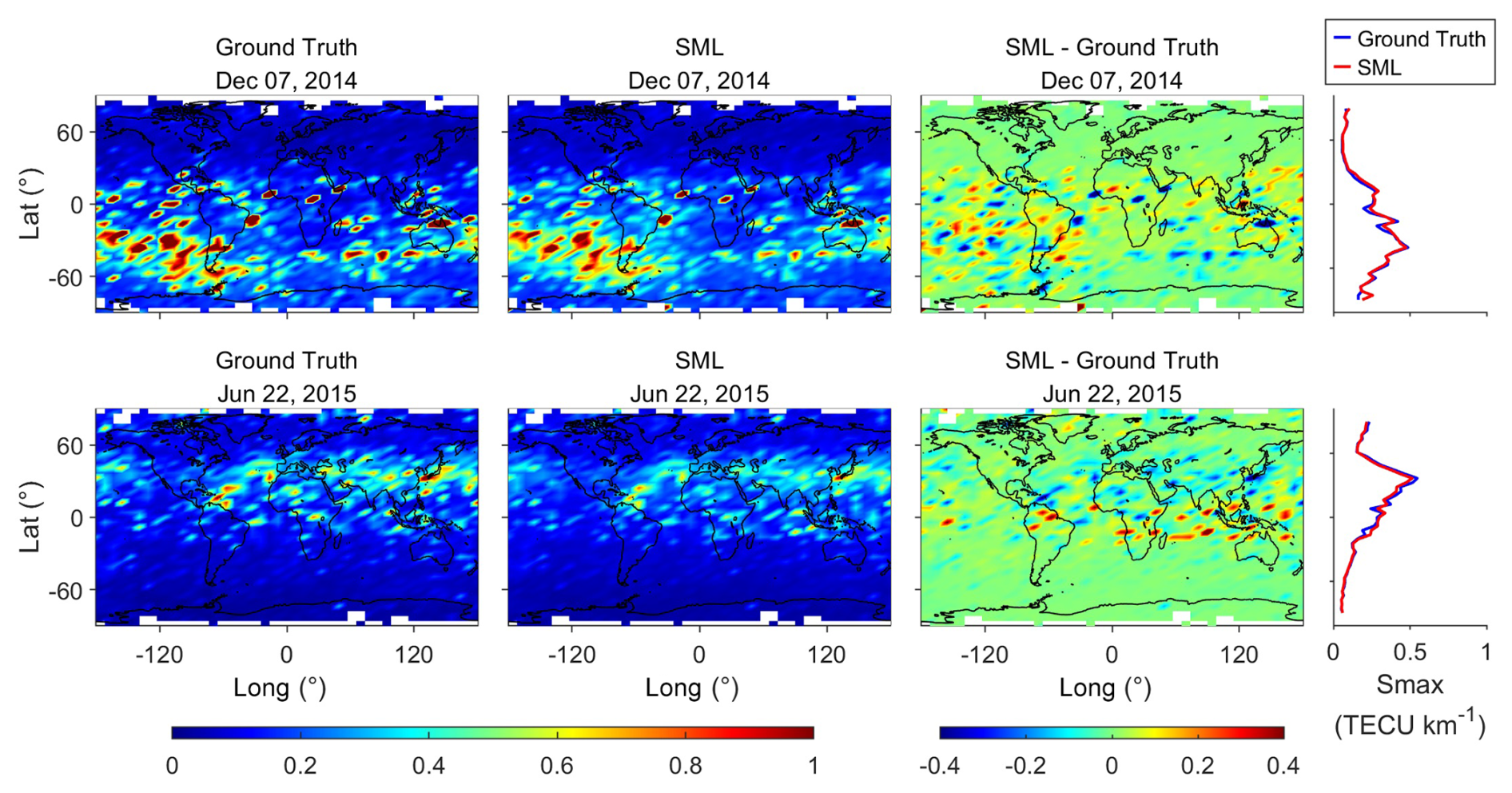
Figure 13 Latitude–longitude and latitudinal distributions of ground truth, SML-predicted EsI, and the corresponding error maps during geomagnetic storm times on 7 December 2014 and 22 June 2015.

Figure 13 shows the latitude–longitude and latitudinal distributions of ground truth, SML-predicted EsI, and the corresponding error maps on 2 storm days, 7 December 2014 (moderate storm, Dst $=-\mathrm{43}$ nT) and 22 June 2015 (major storm, Dst $=-\mathrm{121}$ nT). Compared to quiet days, the EsI distributions during storm days are more complex, showing more irregular patches of EsI enhancement. The general distributions of SML predictions still agree well with ground truth, while there are more outliers in the summer hemisphere and at low latitudes compared to quiet days, as shown in the error maps. The ME/RMSE for the 2 storm days are 0.008/−0.004 and 0.278/0.268 TECU km⁻¹, respectively. In addition, SML has more overestimations of EsI on 7 December 2014, while there are both overestimations and underestimations on 22 June 2015. Liu et al. (2022) reported that EsI usually has a decrease during moderate storms than during quiet times and presents a complex variation during major storms. Although their study is from a climatological perspective, it may explain our prediction results during geomagnetic storms. Nonetheless, Figs. 12 and 13 suggest that the SML model has a reliable ability for short-term EsI prediction under different geomagnetic levels.

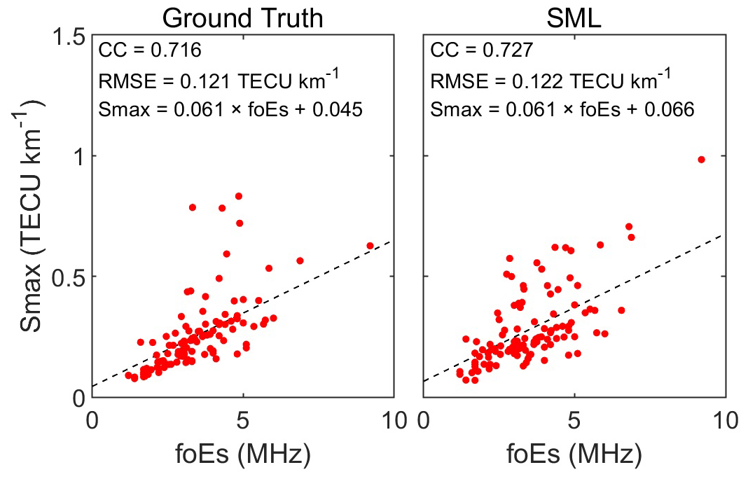
Figure 14 Scatter plots of the matched ground truth and the SML-predicted EsI with ionosonde foEs.

4.4 External validation using ionosonde observations

In the previous empirical modeling of EsI, ionosonde foEs observations are usually used to verify the accuracy of RO measurements (Niu et al., 2019; Hu et al., 2022). To compare the SML-predicted EsI (Smax) and ionosonde foEs on the testing set, they should be matched under a specific spatiotemporal window. Luo et al. (2019) indicated that the influence of the increase in the spatial window on the matching results is much greater than that in the time window. Therefore, we adopt the window of (0.5°, 0.5°, 1 h) to ensure both the amount and consistency of the matched pairs. Figure 14 demonstrates the scatter plots of the matched ground truth and the SML-predicted EsI with ionosonde foEs. The results show that the fitted equation between SML predictions and foEs is much closer to that between ground truth and foEs. The fitted RMSE of 0.122 TECU km⁻¹ for SML is only slightly worse than that of the ground truth of 0.121 TECU km⁻¹, while the CC becomes even better, from 0.716 for ground truth to 0.727 for SML. The high consistency between the metrics of SML predictions and ground truth indicates the good performance of SML.

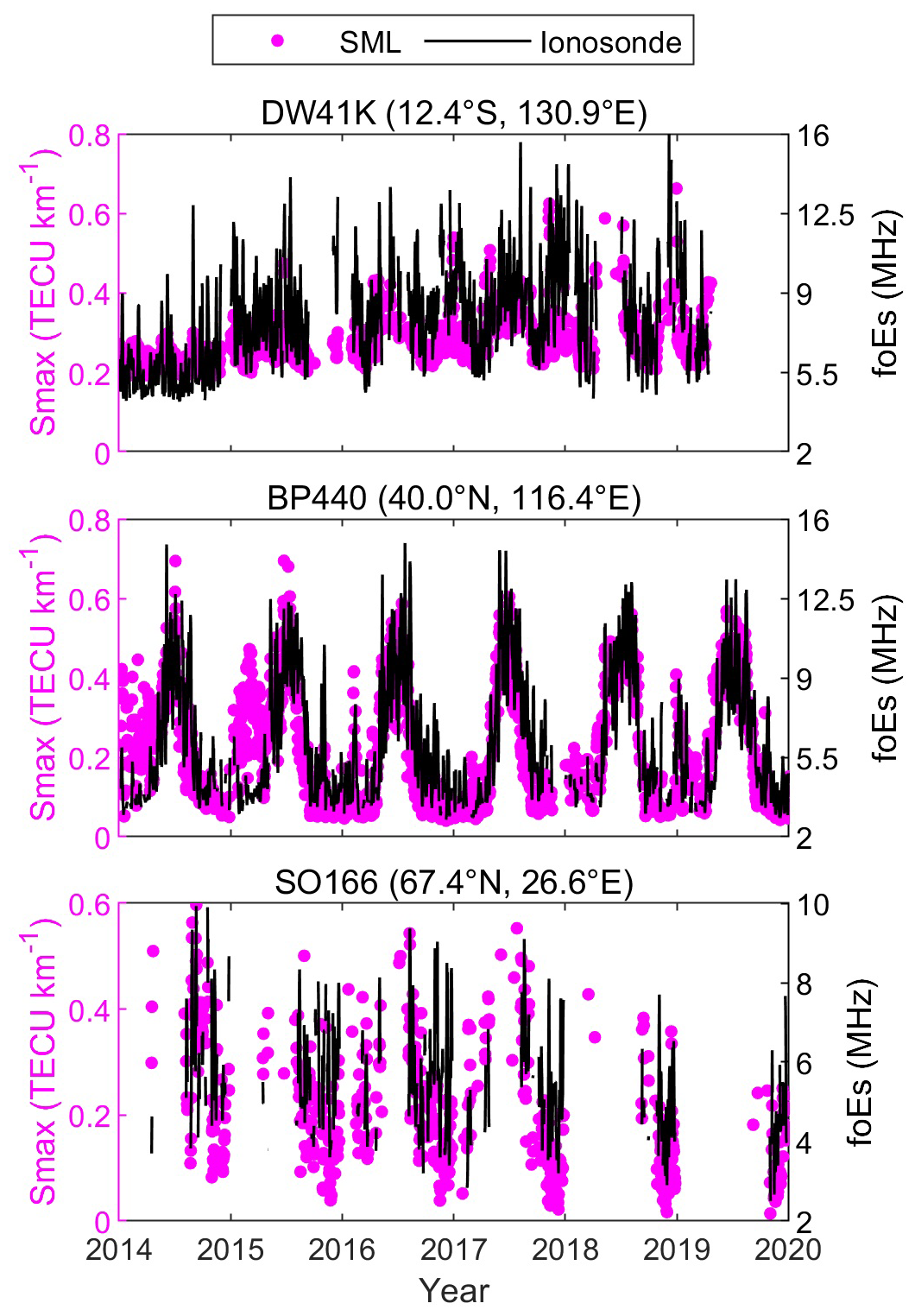
Figure 15 Time series of daily maximum of SML-predicted EsI and foEs over DW41K, BP440, and SO166 ionosondes during 2014–2019.

Furthermore, we verify the consistency of the long-term trends of SML results and ionosonde observations. Three ionosondes located at different latitudes, DW41K, BP440, and SO166, are selected for evaluation. Figure 15 shows the daily maximum of the SML-predicted EsI and foEs over the selected ionosondes during 2014–2019. Note that here EsI and foEs are matched over the location of each ionosonde rather than within the spatiotemporal window. The climatological variations of SML-predicted EsI correspond well with those of the ionosonde foEs in low latitudes, mid-latitudes, and high latitudes. The CCs of SML-predicted EsI and ionosonde foEs over the three ionosondes are 0.613, 0.739, and 0.636, respectively.

Table 1 Metrics of SML with different input variables.

Table 2 Comparison results of EsI estimation models.

5 Discussion

5.1 Advantage of incorporating physical observations in EsI prediction

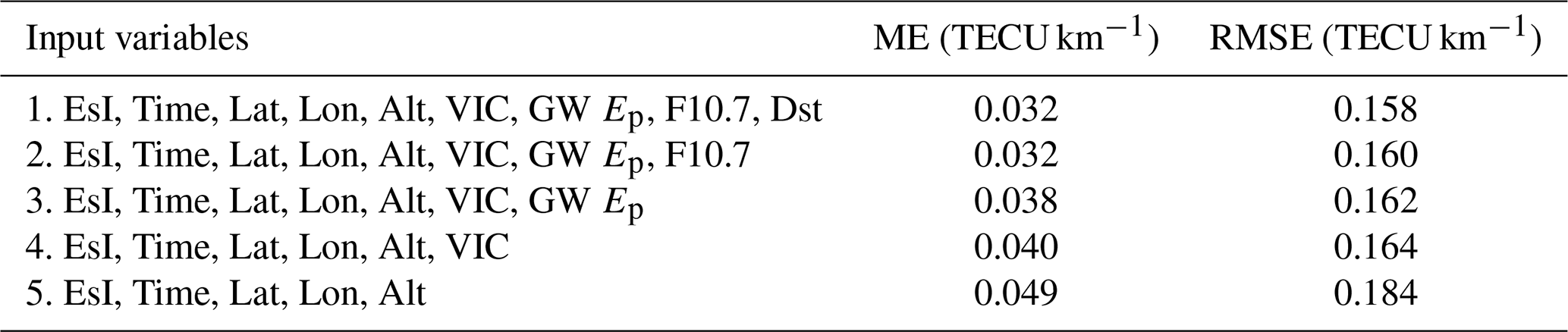
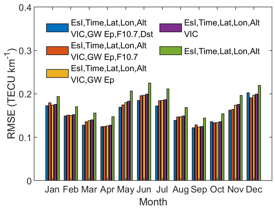
To investigate the effect of incorporating physical observations on the prediction performance of the SML model, we have evaluated the contributions of each physical parameter by removing them from the input variables one at a time. The sequence of removal is Dst, F10.7, GW E_p, and VIC. Table 1 represents the metrics of SML with different input variable combinations on the testing set, which are designated as Combinations 1–5. The models with Combinations 1–4 (with physical parameters) have ME/RMSE smaller than Combination 5 (without physical parameter), and the SML model with Combination 1 has the smallest ME and RMSE compared to other combinations. We can see that after removing each parameter, ME and RMSE generally increase with different magnitudes. The increases are larger after removing VIC and F10.7 (ME of 0.009/0.006 and RMSE of 0.018/0.002 TECU km⁻¹), while they are smaller after removing GW E_p and Dst (ME of 0.002/0.000 and RMSE of 0.002/0.002 TECU km⁻¹), indicating that the contributions of VIC and F10.7 to the model performance are more significant than those of GW E_p and Dst. The possible reason is that the effects of VIC and F10.7 on EsI are on long timescales, such as seasonal, annual, and solar cycles, while GW E_p and Dst tend to impact the small-scale EsI distributions (e.g., hourly or during geomagnetic storms). For example, the relationship between VIC and seasonal/annual variation of E_s layers has been widely revealed based on many observations and simulations (Shinagawa et al., 2017; Qiu et al., 2019; Yu et al., 2019; Luo et al., 2021a; Yamazaki et al., 2022; Ruan et al., 2025), and the variations of EsI and E_s occurrence rate within one solar cycle have also been reported by Bergsson and Syndergaard (2022) and Fontes et al. (2024). In comparison, Qiu et al. (2023) and Liu et al. (2024c) indicated that the modulation of E_s layers by GWs has timescales comparable to the periods of GWs, and there is no significant consistency of the seasonal variation of E_s occurrence with that of GWs. Liu et al. (2022) and Qiu and Liu (2025) pointed out that the downward impacts of geomagnetic storm on the E_s layers mainly occur during the recovery phase. Furthermore, the monthly RMSE of SML with different input variables are shown in Fig. 16. It is evident that the monthly RMSEs of SML with Combination 5 are larger than the SML models with other combinations. The SML with Combination 1 performs better than other models during January–November. The above results show the necessity of incorporating multiple related physical factors to consider the interactions of different atmospheric layers as a coupling system when constructing the E_s prediction model, in which VIC and F10.7 are of significant contributions.

Figure 16 Monthly RMSEs of SML with different input variables.

In recent years, some methods have been proposed for EsI modeling and prediction. Niu and Fang (2023) used COSMIC RO data to develop an empirical model that reproduces the climatological characteristics of EsI at low latitudes and mid-latitudes, with averaged deviation of 0.23 MHz. Emmons et al. (2023) presented two improved prediction model for EsI and demonstrated better performance than those of the empirical models. Although the above methods achieved considerable EsI prediction performance, the lack of E_s-related physical observations limited the further improvements of model accuracy. Tian et al. (2023) conducted the importance ranking of potential E_s-related lower atmospheric parameters (zonal wind, geopotential, temperature, etc.), based on which they selected the input variables for their prediction model, but they did not consider VIC, the most important physical factor. In this study, we comprehensively incorporate VIC, GW E_p, F10.7, and Dst, which have been proven to have significant correlations with EsI. Hence, we have obtained a better performance than the previous models with only the EsI information as inputs.

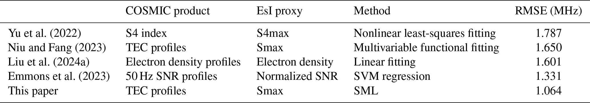
5.2 Comparison of SML and other EsI estimation models

We have collected EsI estimation models using RO measurements from the literature in recent years. These models utilize different COSMIC RO products to derive various EsI proxies using statistical or ML methods. For intuitive comparison, all EsI predictions are validated by ionosonde foEs observations on the same testing set using the same collocation window in Sect. 4.4, and their metric units are all converted to MHz. The comparison results are listed in Table 2. SML has the best prediction performance, and its RMSE is considerably smaller than all the other four models, with improvements of 40.5 %, 35.5 %, 33.5 %, and 20.1 %, respectively. Emmons et al. (2023) used an ML model (SVM regression) to achieve a smaller RMSE than the other three empirical models, while it is still larger than the SML RMSE of this work. This may be due to that single SVM model being not as robust as SML.

6 Conclusions

This study proposes an SML method for global EsI prediction, in which a variety of E_s-related physical observations are incorporated as inputs together with EsI derived from GNSS RO measurements. SML combines the strengths of the optimized base models to obtain lower prediction bias and variance. Taking RO-derived EsI as reference, the ME and RMSE of SML are 0.032 and 0.158 TECU km⁻¹, respectively, and the reductions compared with the maximum ME and RMSE of base models are 39.6 % and 7.1 %, respectively. The evaluation results during 2014–2019 show that SML performs well in the prediction and the characteristics reconstruction of both long-term and short-term EsI variations. Taking ionosonde foEs observations as reference, SML shows better performance in EsI prediction compared to the existing methods, with the RMSE decreases of 20.1 %–40.5 %. Overall, this study presents an effective tool for high-precision global EsI prediction, which can be expected to provide valuable information for ionospheric irregularities monitoring and space weather forecasting. The method's incorporation of multiple E_s-related physical factors is of significant contribution for deepening the understanding of complex interactions between the lower atmosphere, thermosphere, ionosphere, and solar–terrestrial environment.