Evidence of a transient ozone depletion event in the early Hunga plume above the Indian Ocean

On 15 January 2022, the Hunga volcano (20.5° S, 175.4° E) erupted, releasing significant amounts of water vapor (H₂O) and a moderate quantity of sulfur dioxide into the stratosphere. The resulting volcanic plume traveled westward with the southern hemispheric stratospheric circulation, reaching the Indian Ocean and Réunion (21.1° S, 55.5° E) within days. This study presents the first analysis of Infrared Atmospheric Sounding Interferometer (IASI) ozone data to investigate the impact of the Hunga eruption, and also incorporates Microwave Limb Sounder (MLS) and Ozone Mapping and Profiler Suite Limb Profiler (OMPS-LP) data, as well as ground-based measurements from Réunion. IASI observations revealed a transient ozone depletion event in the first week following the eruption. OMPS-LP aerosol extinction profiles, sun-photometer measurements, and lidar observations characterized the plume's vertical and latitudinal extent, showing its presence over Réunion at altitudes ranging from 26.8 to 29.7 km and its spread across more than 30° longitude and 20° latitude by 21 January. IASI ozone spatial distributions showed marked decreases in total and stratospheric ozone on that date, with the fifth percentile of the anomaly reaching −18.6 DU for total column ozone and −14.5 DU for stratospheric column ozone. A key finding, as shown by MLS profiles, is that the ozone reduction was confined to two separate layers ($-\mathrm{0.7}\pm (\mathrm{1}\mathit{\sigma }$) 0.6 ppmv in the 14.68–12.12 hPa range, and $-\mathrm{0.6}\pm (\mathrm{1}\mathit{\sigma }$) 0.5 ppmv in the 31.62–21.54 hPa range), each associated with a distinct aerosol cloud with excess H₂O. This layered structure of ozone loss offers new insight into the chemical and radiative effects of the Hunga plume on stratospheric ozone.

1 Introduction

Due to its high oxidizing potential and contribution to the radiative budget, ozone plays an undeniable role in the Earth's atmosphere (IPCC, 2013, 2021; WMO, 2022). In the stratosphere, ozone serves as a protective shield for the biosphere by absorbing the majority of solar ultraviolet radiation in the 280–315 nm range (Orphal et al., 2016). This shielding action protects ecosystems and human health from the harmful effects of UV-B radiation, which can lead to adverse health issues such as cataracts, melanoma, and skin aging, while deteriorating materials (Pitts et al., 1977; Matsumura and Ananthaswamy, 2004; Bernhard et al., 2020; Neale et al., 2021). In the past decades, anthropogenic emission of chlorofluorocarbons (CFCs) and halons (including Br) was found to be responsible for the rapid decline in stratospheric ozone (Molina and Rowland, 1974; Solomon, 1988; Rowland, 1996). Within the stratosphere, CFCs are photo-dissociated into chlorine compounds, which are known to efficiently deplete ozone (Solomon, 1999). Following the ratification of the Montreal Protocol in 1989, CFC emissions were gradually restricted and forbidden, and previous research and reports show that the ozone layer is expected to return to its 1970s levels from the middle to the end of this century, depending on the latitude (Dhomse et al., 2018; WMO, 2022).

In contrast, tropospheric ozone is a secondary pollutant that directly harms ecosystems, reduces crop productivity, and has negative effects on human health (Mills et al., 2018; Nuvolone et al., 2018). Photochemical formation of tropospheric ozone is driven by the combination of solar radiation and ozone precursors, including volatile organic compounds (VOCs), nitrogen oxides (NO_x) and aerosols (Jacob, 1999; Ivatt et al., 2022). Ozone in the troposphere can therefore be enhanced by anthropogenic activities that release NO_x, aerosols, and VOCs, such as agriculture, industry, and transport.

Explosive volcanic eruptions can influence stratospheric ozone concentrations, and thus play a role in global atmospheric chemistry and radiative forcing (Robock, 2000). Previous major eruptions, such as those of Fuego (1974), El Chichón (1982), Mount Pinatubo (1991), Cerro Hudson (1991), and Calbuco (2015), are well-documented examples of events that have altered global atmospheric chemistry (Crafford, 1975; Cadle et al., 1977; Doiron et al., 1991; Gobbi et al., 1992; Schoeberl et al., 1993; McCormick et al., 1995; WMO, 1999; Guo et al., 2004; Kremser et al., 2016; Zhu et al., 2018). Explosive eruptions can release substantial amounts of sulfur dioxide (SO₂), which is subsequently converted into sulfuric acid (H₂SO₄). The resulting sulfuric acid condenses to form sulfate aerosols, secondary volcanic particles which can in turn contribute to stratospheric ozone depletion by increasing the surface area available for heterogeneous reactions. Studies have highlighted the relationship between SO₂ and chlorine in causing ozone decline post-eruption (e.g., Hofmann and Solomon, 1989; Tie and Brasseur, 1995). As an example, McCormick et al. (1995) reported that tropical column ozone decreased by 6 %–8 % in the months following the Mount Pinatubo eruption. They observed that losses were greatest below 28 km, amounting to 20 % in the 24–25 km altitude range. Because of the resulting ozone losses and radiative forcing anomalies, the injection of volcanic plumes into the stratosphere can also influence atmospheric temperatures. Ramaswamy et al. (2006) observed increases in global lower stratospheric temperatures following the major eruptions of El Chichón and Mount Pinatubo. Moreover, it was determined that the ozone depletion in the aerosol layer caused by the Mount Pinatubo eruption reduced stratospheric heating by 30 % (Kirchner et al., 1999). Despite this reduction, the radiative anomalies caused by the presence of stratospheric aerosols induced a global stratospheric warming of 3–4 K and tropospheric cooling (Stenchikov et al., 1998; Kirchner et al., 1999).

Moderate and major eruptions may also contribute to the amplitude and dimension of the ozone hole over Antarctica. Following the Mount Pinatubo eruption, Hofmann and Oltmans (1993) observed unusually low total ozone values of 105 DU over the South Pole Station. This deeper ozone hole was attributed to enhanced polar stratospheric cloud volume driven by extra stratospheric sulfuric acid availability, offering more particle surfaces for heterogeneous reactions. Ivy et al. (2017) reported an increase of the 2015 Antarctic ozone hole by 4.5×10⁶ km², primarily attributed to volcanic aerosols from the Calbuco eruption. Similarly, Zhu et al. (2018) reported penetration of volcanic sulfate aerosols from the Calbuco eruption into the Antarctic polar vortex, resulting in earlier ozone loss and an increase in the area of the ozone hole. Yook et al. (2022) also hypothesized a link between the eruption of La Soufrière in 2021 and the longevity of the 2021 ozone hole. Hence, numerous research papers focused on ozone chemistry and atmospheric forcings following eruption events.

The Hunga eruption constitutes an unprecedented event of the satellite era (Wright et al., 2022; Carr et al., 2022). The main eruption likely released more energy than the 1991 Mount Pinatubo eruption and caused the largest stratospheric aerosol disturbance since that event (Sellitto et al., 2022; Khaykin et al., 2022; Taha et al., 2022). Its consequences have been under intensive scrutiny, and studies revealed it injected ∼0.5 Tg of SO₂ and 146±5 Tg of water vapor (H₂O) into the stratosphere, corresponding to an increase of ∼10 % of the global stratospheric H₂O burden (Khaykin et al., 2022; Vömel et al., 2022; Zuo et al., 2022; Millán et al., 2022). The eruption's aerosol column extended through the troposphere and stratosphere, and even reached the lower mesosphere (Carr et al., 2022). Legras et al. (2022) demonstrated that the initial volcanic plume consisted of two distinct sulfate aerosol clouds, which descended from ∼30 and ∼28 km on 15 January to ∼27 and ∼25 km by 28 January.

Evan et al. (2023) and Zhu et al. (2023) attribute the initially low ozone levels observed in satellite data to the lofting of ozone-poor tropospheric air masses. However, the subsequent ozone depletion in the following days is attributed to chemical processes, particularly heterogeneous chlorine activation on humidified volcanic aerosols. The significant increase in stratospheric humidity facilitated the rapid conversion of SO₂ to sulfate aerosols in less than two weeks (Legras et al., 2022; Asher et al., 2023; Zhu et al., 2022, 2023), increasing aerosol surface area. This, combined with Hunga-induced stratospheric cooling (Sellitto et al., 2022; Coy et al., 2022; Schoeberl et al., 2022; Sicard et al., 2025), enhanced heterogeneous reaction rates, likely accelerating chlorine activation on sulfate aerosols and leading to notable ozone depletion despite elevated non-polar temperatures (Evan et al., 2023; Zhu et al., 2023). In this context, Evan et al. (2023) provided evidence of HCl activation on sulfate aerosols within the fresh volcanic plume, and Zhu et al. (2023) elucidated the mechanisms giving rise to the changes observed immediately following the event. (For completeness, note that comprehensive discussions of the stratospheric chemical processes at work in subsequent months can be found in Wilmouth et al., 2023, Santee et al., 2023, and Zhang et al., 2024b.)

While heterogeneous reactions played a crucial role in ozone loss, Zhu et al. (2023) also emphasized the importance of gas-phase reactions. In fact, Zhu et al. (2023) and Evan et al. (2023) identified key gas-phase mechanisms contributing to ozone loss: enhanced HO_x cycle activity due to high H₂O concentrations, as highlighted also by Wilmouth et al. (2023), strengthened interactions between the HO_x and ClO_x cycles (through ${\text{HO}}_{\mathrm{2}}+\text{ClO}\to \text{HOCl}+{\mathrm{O}}_{\mathrm{2}}$), and the slowing down of the NO_x cycle. During the 2022 austral springtime and wintertime, the slowdown of the NO_x cycle gave rise to ClO_x enhancements (Zhang et al., 2024a). According to Zhang et al. (2024a), the impact on ozone from the reduction of the NO_x cycle was largely offset by enhanced HO_x and ClO_x cycles.

Thus, the substantial increase in the rates of key reactions led to a 5 % decrease in stratospheric ozone over the Indian Ocean within a week of the eruption, as reported by Evan et al. (2023), with the most pronounced losses occurring during peak stratospheric humidification.

This study provides the first analysis of ozone observations using Infrared Atmospheric Sounding Interferometer (IASI; Aires et al., 2002; Blumstein et al., 2004) data following the January 2022 Hunga eruption, focusing on the Indian Ocean and particularly Réunion, where our ground-based measurements are performed. Due to the prevailing westward austral summer stratospheric circulation, the first signs of the Hunga plume's passage over Réunion were noticed only 4 d after the eruption (Legras et al., 2022; Baron et al., 2023). This study combines local ground-based measurements at Réunion with satellite data over the Indian Ocean, including observations from the Microwave Limb Sounder (MLS; Waters et al., 2006) and IASI, to examine the impacts of Hunga on ozone during the first 10 d post-eruption. The goal is not to elucidate the chemical mechanisms giving rise to the observed low ozone, as they were investigated in detail by Evan et al. (2023) and Zhu et al. (2023). Rather, the objectives of the present manuscript can be summarized in three points: firstly, we use IASI observations to demonstrate the appearance of a transient ozone depletion event; secondly, we show the zonal displacement of the SO₂ and H₂O plumes using satellite data; and thirdly, we use MLS ozone profiles obtained within each of the two Hunga clouds to characterize their respective impacts on ozone.

2 Instrumentation and method

In this study we combined ground-based and satellite observational data to investigate the impacts on ozone after the Hunga eruption. This work focuses on the region bounded by 45–175° E and 30–0° S, and relies on satellite measurements obtained exclusively within this area. This section outlines the different types of data used in our analysis. Unless specified otherwise, all uncertainties, standard errors, and standard deviations are reported at the 2σ confidence level.

2.1 Ozone measurements

2.1.1 Lidar

A stratospheric DIfferential Absorption Lidar (DIAL) has been operated since January 2013 at the Réunion Atmospheric Physics Observatory (OPAR, 21.08° S; 55.38° E, 2160 $\mathrm{m}\mathrm{a}.\mathrm{s}.\mathrm{l}.$; Baray et al., 2013; Portafaix et al., 2015). This instrument can retrieve ozone concentration profiles at altitudes ranging from 15 to ∼45 km. Lidar observations provide high vertical resolution (Pazmiño, 2006), with typical values ranging from 0.5 at 15 km to 5 at 45 km (Godin-Beekmann et al., 2003). The total accuracy is ∼5 % below 20 km, ∼3 % in the 20–30 km altitude range, and 15 %–30 % above 45 km (Godin-Beekmann et al., 2003). However, although the Maïdo DIAL system recorded data during the initial passage of the volcanic plume in January 2022, the corresponding signal-to-noise ratio (SNR) was extremely low, and the ozone profiles were not reliable. As a result, stratospheric DIAL ozone profiles used in this paper were recorded before the Hunga eruption, from January 2013 to December 2021. The 470 ozone profiles obtained during this period were used to determine the background ozone level for the month of January and were compared with profiles from satellites. As part of the Network for the Detection of Atmospheric Composition Change (NDACC), this DIAL data can be accessed from the NDACC website (https://ndacc.larc.nasa.gov/, last access: 10 March 2025).

2.1.2 SAOZ

The Système d'Analyse par Observation Zénithale (SAOZ), an instrument also integrated into the NDACC, is a ground-based spectrometer that measures the sunlight scattered from the zenith sky within the 300–650 nm range (Pommereau and Goutail, 1988). Differential optical absorption spectrometry is utilized to analyze observations, enabling the retrieval of daily ozone and nitrogen columns at sunrise and sunset with a total accuracy of 6 % and 14 %, respectively (Boynard et al., 2018). Operating at an altitude of 80 $\mathrm{m}\mathrm{a}.\mathrm{s}.\mathrm{l}.$ in Saint-Denis (20.90° S; 55.48° E), Réunion, since 1993, a SAOZ instrument has provided total column ozone (TCO) observations at this subtropical site for over three decades. Unfortunately, SAOZ data during the passage of the aerosol plume over Réunion are unreliable because of an unrealistic representation of the air mass factor, leading to biased TCO retrievals. Consequently, SAOZ data for January 2022 were excluded. However, data outside this time period and climatological values of TCO for the month of January (262.8±11.9 DU) were kept to illustrate the background January TCO. The dataset used in this work can be downloaded from the SAOZ website (http://saoz.obs.uvsq.fr/, last access: 10 March 2025).

2.1.3 MLS

The MLS instrument is aboard the Aura satellite, which was launched in July 2004. The Aura satellite follows a helio-synchronous orbit and passes the Equator at 13:45 local solar time on its ascending node. In order to observe atmospheric parameters like temperature and atmospheric component concentrations, MLS measures thermal radiation emitted from the Earth's atmospheric limb ahead of its orbital path at spectral wavelengths ranging from 0.12 to 2.5 mm (Waters et al., 2006). According to Millán et al. (2022), MLS version 4 (v4) level 2 data should be used to study conditions within the fresh Hunga plume for the first three weeks after the eruption instead of the latest version (v5). Indeed, the extraordinary H₂O enhancement from Hunga compromised the accuracy of some v5 MLS data products immediately after the eruption. However, their study indicates that the quality of MLS ozone and temperature measurements are not affected by the volcanic plume (Millán et al., 2022).

Following the recommendations of Millán et al. (2022), the MLS profiles for January 2022 are sourced exclusively from level 2 v4 measurements (Livesey et al., 2020). The MLS profiles are categorized as Hunga-influenced or non-influenced using criteria detailed in the next paragraph. To evaluate the similarity between v4 and v5 MLS ozone profiles during background atmospheric conditions, we calculated the differences for the colocated v4 and v5 non-influenced ozone profiles. The maximum standard deviation did not exceed 0.1 ppmv on any of the 10–100 hPa pressure levels, corresponding to a 0.02 % variation relative to the mean ozone volume mixing ratio in this region, demonstrating the similarity of these two versions during background conditions. Additionally, to assess the similarity between v5 MLS ozone profiles and the Réunion DIAL profiles, we performed an inter-comparison procedure detailed in Sect. 2.4. To compare v4 Hunga-influenced ozone profiles to background non-influenced profiles, we employed MLS level 2 v5 data (Livesey et al., 2022). All v5 ozone and water vapor profiles (on both ascending and descending sides of the orbit) within a 5° radius of each of the January 2022 Hunga-influenced profiles were collected. This procedure was undertaken for each day for the months of January from 2013 to 2021 to derive the monthly averaged background profiles. This specific time period was chosen to align with the lidar time series.

The selection of v4 MLS Hunga-influenced profiles follows an adaptation of the criterion from Evan et al. (2023). First, similar to their procedure, locations with v4 water vapor profiles exhibiting mixing ratio values exceeding 100 ppmv within the 10–100 hPa range were identified. Based on Legras et al. (2022), the criterion was then refined to classify as Hunga-influenced only those profiles affected by one of the two sulfate aerosol clouds located at approximately 25 and 28 km (corresponding to the 26.10 and 14.68 hPa MLS pressure levels, respectively). Specifically, only profiles in which the maximum H₂O anomaly occurred at one of these two pressure levels were considered to be Hunga-influenced. This refinement accounts for the fact that, during the study period (15–23 January 2022), water vapor and aerosol plumes were colocated before diverging due to particle sedimentation. These two separate plumes of water vapor and aerosols are referred to as “Hunga clouds.” Applying this refined criterion yielded 47 Hunga-influenced and 2266 non-influenced ozone and water vapor profiles between 15 and 23 January 2022 over the Indian Ocean. Of the Hunga-influenced profiles, 26 were impacted by the higher-altitude cloud, and 21 by the lower-altitude one. The two profile groups were analyzed separately to characterize the individual impacts of each Hunga cloud on ozone.

In most of the stratosphere, specifically between 1 and 68 hPa, MLS ozone volume mixing ratio profiles have accuracy and precision that are both better than 10 % (Livesey et al., 2022). In accordance with the recommendations made in the MLS data quality and description documents, all quality flags (quality, convergence, status, and precision) were used on the raw ozone profiles, and data lying outside the recommended range (261–0.001 hPa, or approximately 11–90 km) were not used (Livesey et al., 2020, 2022). MLS observations can be accessed through NASA's data portal (https://disc.gsfc.nasa.gov/, last access: 10 March 2025).

2.1.4 IASI

In 2006, the first IASI was launched aboard the Metop-A satellite (Clerbaux et al., 2009; Coheur et al., 2009). A second instrument was launched in 2012 on Metop-B, followed by a third on Metop-C in 2018. These satellites operate in a polar orbit, providing global observations twice a day (09:30 and 21:30 LT) for weather prediction and climate monitoring. IASI is a Fourier transform spectrometer, which measures the radiation emitted by the Earth-atmosphere system in the thermal infrared (645–2760 cm⁻¹ or 3.62–15.5 µm) across 8461 spectral channels, with a resolution of 0.25 cm⁻¹ (0.5 cm⁻¹ after apodization). IASI's swath covers 30 fields of view, each containing 4 pixels, allowing for complete Earth coverage during each pass.

In this study we used the IASI ozone profiles retrieved from Fast-Optimal Retrievals on Layers for IASI (FORLI; Hurtmans et al., 2012), which have been extensively validated (Boynard et al., 2018) and which are available to users on the AERIS website (https://iasi.aeris-data.fr, last access: 10 March 2025). The ozone product is a vertical profile given as partial columns in molecules cm⁻² in 40 layers between the surface and 40 km, with an extra layer from 40 to ∼60 km. To ensure that only the most reliable observations are used in our analysis, we applied a filtering process, retaining only profiles and columns with more than two degrees of freedom and a retrieval quality filter equal to 1, as recommended by Boynard et al. (2018). We analyzed both the TCO and stratospheric column ozone (SCO) products. The latter is derived by summing the ozone partial columns from the thermal tropopause, estimated from the IASI temperature profiles using the World Meteorological Organization (WMO) definition (World Meteorological Organization, 1957), to ∼60 km.

As Metop-A began its orbital drift in 2017 and stopped providing measurements in 2021, only IASI/Metop-B and -C have been used in this study. To facilitate the analysis, the IASI TCO and SCO data were first averaged daily over a 1°×1° global grid. The background ozone levels were defined as the daily average of IASI/Metop-B data from 2014 to 2021. The daily ozone values for 2022 were derived from both Metop-B and -C to maximize the number of data points. IASI TCO and SCO anomalies were defined as the difference between the daily ozone levels in January 2022 and the background daily ozone (average between 2014 and 2021 for January). To ensure statistical reliability for the ozone anomalies, only grid points with at least three observations were considered.

To complement the analysis, we also included daily SO₂ measurements from IASI/Metop-B and -C (Clarisse et al., 2012, 2014). Regional ozone anomalies were investigated by isolating data points within the SO₂ plume, as detected using IASI SO₂ measurements. To identify regional depletion events, we computed the fifth percentile of ozone anomalies across all points within the SO₂ plume.

In contrast to UV–visible instruments, which reported significant perturbations in their ozone retrievals following the eruption (attributed to interference from SO₂ and H₂SO₄), no similar disturbances were observed in the IASI ozone retrievals. Because the spectral ranges used for ozone and SO₂ in the IASI retrieval algorithms do not overlap, results should not show any bias. Although sulfate aerosols may share some spectral range with ozone, the retrieval algorithm can effectively distinguish between the two, as sulfate aerosols exhibit strong absorption features and ozone variations are directly measured through its absorption lines. Thus, the IASI algorithm should account for ozone variability effectively following the Hunga eruption.

2.2 Aerosol measurements

In addition to the DIAL system, the OPAR is equipped with several other active remote sensing systems, including a Rayleigh–Mie lidar for aerosol profile measurements (Baron et al., 2023). In this study we used aerosol extinction profiles together with the corresponding stratospheric aerosol optical depth (sAOD) at 532 nm as derived from the Rayleigh–Mie lidar measurements at the Réunion observatory. The data used in this study, which are publicly accessible via the Geosur website (https://geosur.osureunion.fr, last access: 10 March 2025), are also available as a ready-to-use dataset from Baron (2023).

Aerosol optical properties can also be retrieved using sun-photometers. These remote sensing sun-tracking radiometers perform regular and frequent measurements of the direct solar spectral irradiance, typically at wavelengths between 340 and 1640 nm. By comparing the ground solar irradiance to the estimated top-of-the-atmosphere irradiance, they can determine the total AOD, a quantity that describes the opacity of the atmosphere to radiation. Therefore, a sun-photometer gives a measure of aerosol abundance in the atmospheric column above the study site. In the present study, we used AOD data from a Cimel sun-photometer located at the Saint-Denis campus, which has been operating since December 2003 in the framework of the AErosol RObotic NETwork (AERONET) program. We used level 2.0 v3 AERONET data for the period from December 2003 to January 2022. AERONET data of level 2.0 is quality-controlled with near-real-time automatic cloud-screening in addition to having pre- and post-field calibrations. According to Giles et al. (2019), the 1σ uncertainty for the near-real-time AERONET AOD measurement is up to 0.02. The data are available from the AERONET website (https://aeronet.gsfc.nasa.gov/, last access: 10 March 2025).

The Ozone Mapping and Profiler Suite Limb Profiler (OMPS-LP) monitors the Earth limb ahead of its orbit path to provide high-vertical-resolution ozone and aerosol profiles. The instrument measures limb scattering radiances in the 290–1000 nm wavelength range over the sunlit portion of the atmosphere using three vertical slits. This instrument has been making observations onboard the Suomi National Polar-orbiting Partnership (Suomi NPP) spacecraft since January 2012, following a helio-synchronous orbit with an equatorial passing time of 13:30 solar time on its ascending node. With the goal of studying the spatial extension of the plume, we used OMPS-LP aerosol extinction profiles at 745 nm. According to Taha et al. (2021), extinction coefficients at 745 nm have relative accuracy and precision of 10 % and 15 %, respectively. The OMPS data used in this study are available from the Goddard website (https://ozoneaq.gsfc.nasa.gov/, last access: 10 March 2025).

2.3 Trajectory model

To investigate the origin of the air masses in our study region, we used the HYbrid Single Particle Lagrangian Integrated Trajectory (HYSPLIT) model in its passive and backward mode (Draxler and Hess, 1997, 1998). Developed by the National Oceanic and Atmospheric Administration (NOAA), this model uses meteorological fields to compute trajectories of air masses. We used a single HYSPLIT simulation to track stratospheric air mass trajectories over the Indian Ocean. Thus, using meteorological fields from the Global Data Assimilation System (GDAS; National Oceanic and Atmospheric Administration (NOAA), 2023), we ran a 240 h back trajectory simulation of 12 distinct air parcels with terminal altitudes distributed equally between 23.5 and 29.0 km. These trajectories were chosen to have their endpoint at the location of Saint-Denis, Réunion. HYSPLIT trajectories can be obtained by running simulations via the HYSPLIT website (https://www.ready.noaa.gov/HYSPLIT_traj.php, last access: 10 March 2025).

2.4 Inter-comparison

Prior to drawing any conclusions based on the MLS ozone profiles, we compared them with Maïdo DIAL observations during background atmospheric conditions, representing a new contribution to the evaluation of MLS data in this region. For this inter-comparison process, we calculated daily MLS ozone profiles by averaging all profiles within a 5° region around the lidar site. We averaged together MLS v5 ozone profiles from both the ascending and the descending sides of the Aura orbit, which have acquisition times near Réunion around 10:15 and 21:45 UTC, respectively. On the other hand, the 470 ground-based DIAL lidar profiles are only nocturnal (recorded at Réunion, i.e., between approximately 16:00 and 01:00 UTC, averaging around 18:30 UTC). Thus, the maximum temporal difference between MLS and lidar profiles is approximately 8 h. Despite the non-overlapping acquisition times, we compared DIAL night profiles to daily MLS profiles. Although we obtained 470 DIAL profiles, the 5° inter-comparison radius limits the number of available MLS profiles, allowing inter-comparison on a total of 340 d. Since lidar profiles use altitude as the vertical coordinate and MLS retrievals are output on a pressure grid, we first converted the MLS pressure grid to an altitude grid using MLS geopotential height profiles. Following Sects. 1.8 and 1.9 of Livesey et al. (2022), the comparison with lidar profiles was conducted by applying MLS averaging kernels and a priori ozone profiles, after reducing the resolution of the lidar profiles using least-squares smoothing. As a result, the profile comparison is based on the relative difference between the two datasets, as defined by the following formula:

$$\begin{array}{}\text{(1)}& {\displaystyle }{\displaystyle }{\text{Relative}}_{\text{bias}}\left(z\right)=\mathrm{100}\times {\displaystyle \frac{{\mathrm{O}}_{\text{3\hspace{0.17em}MLS}}\left(z\right)-{\mathrm{O}}_{\text{3\hspace{0.17em}DIAL}}\left(z\right)}{{\mathrm{O}}_{\text{3\hspace{0.17em}DIAL}}\left(z\right)}},\end{array}$$

where O_3 MLS(z) represents the MLS ozone value at altitude z and O_3 DIAL(z) represents the smoothed stratospheric DIAL ozone value at the same altitude. Other statistical quantities were also determined, namely the number of profiles (N), the coefficient of correlation (r), the linear regression (in the form y=ax), and the root-mean-square deviation (RMSD). These statistical quantities were used to assess the differences and similarities between different ozone data in different layers.

Additionally, to compare IASI data with SAOZ measurements at Réunion under background atmospheric conditions, we derived a daily TCO time series from Metop-B at Réunion, spanning March 2013–December 2021. The inter-comparison utilized all data points from both datasets within this time period, irrespective of date and time of day, including all sunrise and sunset measurements.

3 Results and discussion

3.1 Aerosol plume

The Hunga main eruption occurred on 15 January 2022 and injected a large quantity of H₂O and a moderate amount of SO₂ into the stratosphere (Khaykin et al., 2022; Sellitto et al., 2022; Zuo et al., 2022; Millán et al., 2022). Following the austral summer's general stratospheric circulation, the volcanic plume then traveled westward and reached the Indian Ocean and the African continent within days (Baron et al., 2023). The aerosol plume's transport across the Indian Ocean was captured by OMPS aerosol extinction profiles. Figure 1a shows the background aerosol distribution at 745 nm over the Indian Ocean, captured prior to the arrival of the volcanic plume. Panels b–e present OMPS extinction coefficient profiles across different locations in the Indian Ocean as a function of latitude and altitude during the passage of the volcanic plume. At the bottom left of each panel are given the date and time of retrieval; the black dots correspond to the thermal tropopause estimated from the OMPS-LP temperature data using the WMO definition (World Meteorological Organization, 1957) and the vertical dashed lines mark the positions of the 5 and 25° S latitude lines. Panel f traces the satellite tracks corresponding to data in panels a–e. Thus, this figure describes the latitudinal and vertical extent of the volcanic plume as observed by the satellite instrument during its passage over the Indian Ocean on 22 January, the date when impacts on ozone at Réunion were highest (Evan et al., 2023). During background atmospheric conditions (see Fig. 1a), the aerosol distribution shows that the largest values of the extinction coefficient are kept below the tropopause. Aerosol presence in the stratosphere is negligible compared to that in the troposphere. However, the presence of the volcanic plume becomes clearly visible on the other panels, where large extinction coefficient values ($>{\mathrm{10}}^{-\mathrm{3}}$) lie above the tropopause level and become comparable to those typically observed in the upper troposphere. On 22 January (Fig. 1b–e), the volcanic plume is clearly visible in the stratosphere over the Indian Ocean between 5° and 25° S, reaching altitudes greater than 35 km. Note that this result only characterizes the vertical and latitudinal extent of the volcanic plume, but it does not describe the longitudinal dimension of the plume. Equivalent observations can also be obtained for 21 January (not shown). Similar results were found by Taha et al. (2022) as they outlined the presence of a volcanic plume located at an altitude exceeding 36 km. Additionally, they reported that the high sensitivity of OMPS-LP enabled the monitoring of the volcanic plume at altitudes above 36 km for a duration of up to 90 d.

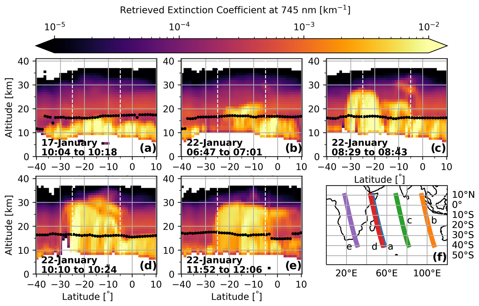
Figure 1 OMPS-LP aerosol extinction height–latitude cross-sections over the Indian Ocean at 745 nm for (a) background conditions on 17 January prior to the passage of the volcanic plume and (b–e) during the passage of the plume on 22 January. (f) shows the satellite track corresponding to each overpass. The superimposed black dots on (a–e) indicate the tropopause altitude estimated from the OMPS-LP temperature data, using the WMO definition (World Meteorological Organization, 1957). Vertical dashed lines mark the positions of the 5° and 25° S latitude lines.

Figure 2 shows the Hunga aerosol plume as seen by two quasi-colocated instruments operating at the Maïdo observatory (lidar) and the Saint-Denis campus (sun-photometer). It is important to emphasize that the two instruments are 20 km apart with an approximately 2000 m difference in elevation. Even though the total AOD measured by the sun-photometer cannot be directly compared to the sAOD recorded by the lidar instrument, both sets of observations hold significant information about the passage of the volcanic plume. Figure 2a depicts the evolution of the lidar aerosol extinction profiles at 532 nm between 21 and 23 January, and Fig. 2b shows the evolution of the lidar sAOD at 532 nm (in black) and sun-photometer level 2.0 total AOD at 532 nm (in red) for the second half of January 2022. The lidar sAOD uncertainty is represented by the gray shading, while the sun-photometer AOD uncertainty, assumed to be about 0.02 (1σ) for all measurements (Giles et al., 2019), is illustrated in the upper part of the panel at the 2σ level. The sun-photometer AOD at 532 nm was obtained from the conversion of the AOD at 675 nm using the Ångström exponent measurements between 440 and 675 nm. The blue line represents the multi-year average of sun-photometer level 2.0 AOD data for January, calculated from 2003 to 2021, with the shaded blue region indicating the corresponding standard deviation. Note that different horizontal axes are used for panels a and b, and the common observation periods are enclosed by vertical dashed lines in the two panels.

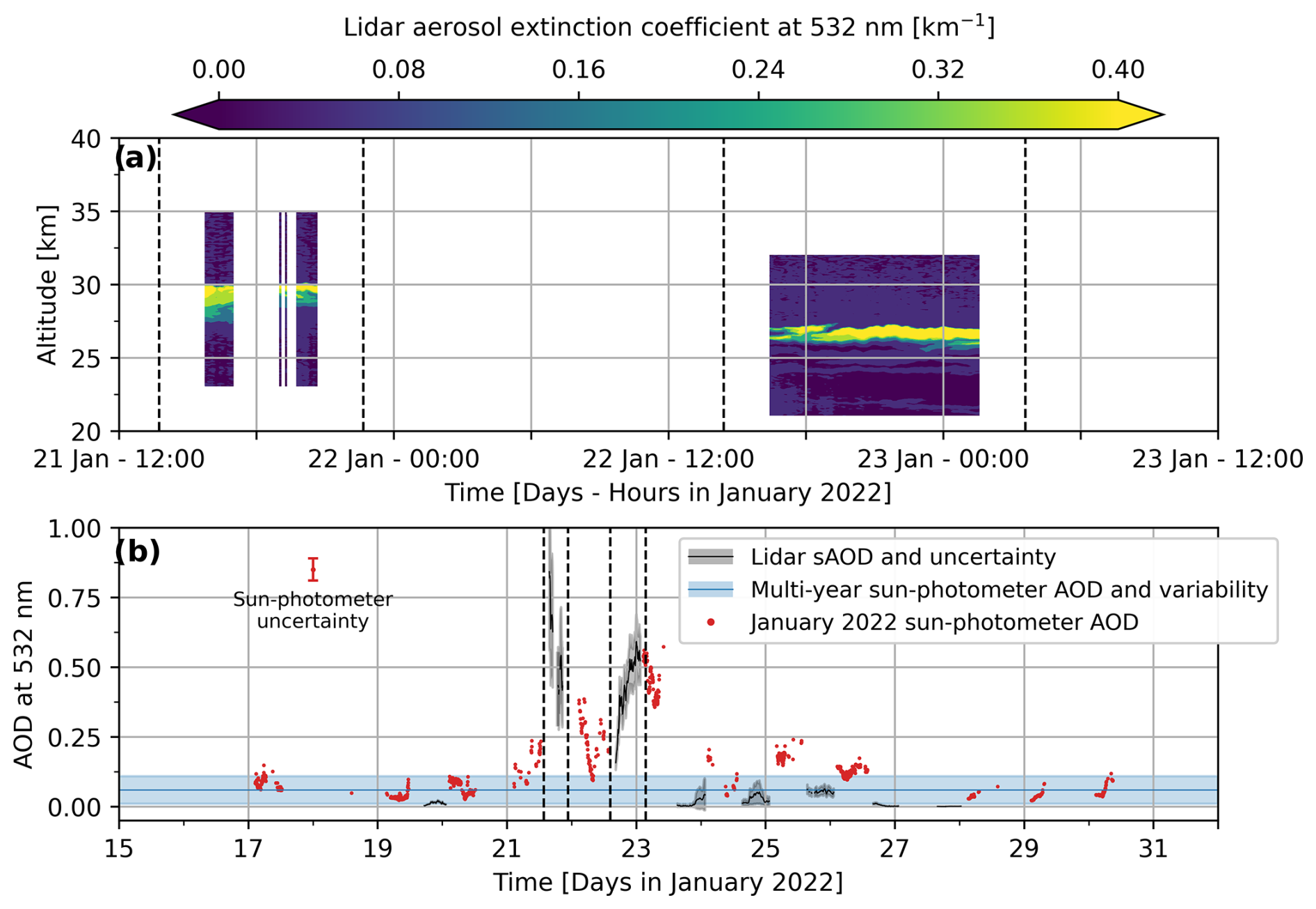
Figure 2 (a) Aerosol lidar extinction profiles at 532 nm and (b) aerosol lidar stratospheric AOD (sAOD) in black with level 2.0 sun-photometer total AOD in red. The gray shading indicates the lidar sAOD uncertainty, while the sun-photometer total AOD uncertainty is illustrated in the upper part of (b). The blue line and shaded area represent average and standard deviation values given by level 2.0 sun-photometer data from the months of January taken between 2003 and 2021. The common observation periods in the two panels are visually represented with vertical dashed lines.

Results in Fig. 2b show that the maximum total and stratospheric optical depths recorded by the two instruments in January 2022 are very high in comparison to the multi-year mean AOD of 0.05±0.04. This is expected, as Réunion is a pristine region where January usually experiences low AOD levels (Duflot et al., 2022). After 20 January, total AOD values start to dramatically increase until 23 January, when they culminated at 0.57±0.04 before gradually decreasing to return to background levels. Similar to the sun-photometer measurements, the Maïdo lidar reveals a large amount of aerosols after 21 January, with sAOD values rising up to 0.84±0.27. A significant aerosol layer was seen by the lidar on two consecutive nights at altitudes of 29.7 and 26.8 km, with maximum extinction coefficients of 0.53±0.17 and 0.68±0.11, respectively (see Fig. 2a). Note that sun-photometer measurements are obtained during the day, while lidar observations are only performed during nighttime. As such, observations from these two instruments cannot overlap as they do not operate simultaneously. A detailed study of the lidar observation of the Hunga plume can be found in Baron et al. (2023). Our results support their research, suggesting that the bulk of the Hunga aerosol plume passed over Réunion from 21 to 23 January.

3.2 Maïdo DIAL and MLS average ozone profiles

Figure 3 shows the average January Maïdo DIAL ozone profile, with the blue shaded area indicating the standard deviation. The orange and green lines represent the average January MLS ozone profiles representative of Réunion and the full study region, respectively, with standard deviations shown as horizontal bars. The averages of all profiles remain within each other's standard deviation. Above 37 km, the average lidar profile slightly diverges from the average MLS profiles, likely due to decreased lidar SNR and fewer available profiles, which also increases the standard deviation. Still, the average profiles are similar in the 15–37 km range. Because of the similarity between the lidar and MLS average ozone profiles over Réunion up to ∼30 km (the altitude of the higher Hunga cloud), MLS data are a suitable substitute for lidar data, as expected.

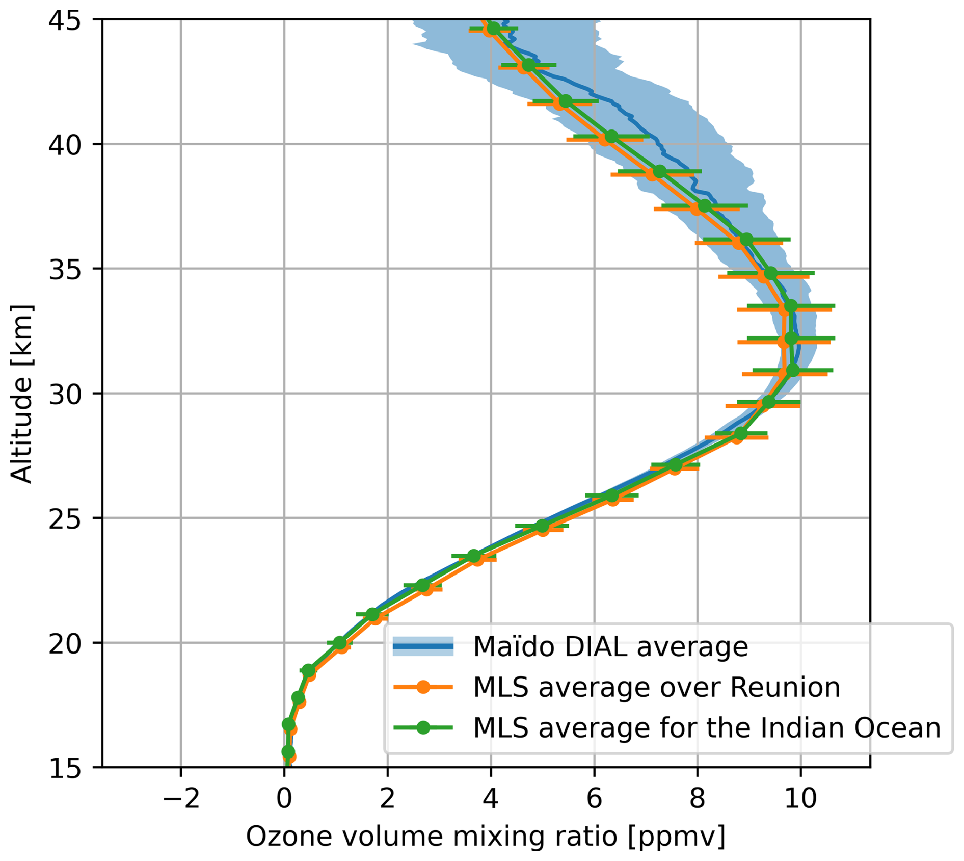
Figure 3 Average January stratospheric DIAL profile calculated from observations taken over 2013–2021 at Réunion (blue), alongside average January MLS profiles for Réunion (orange) and the full study region (green). Standard deviations are shown as a shaded region for the DIAL profile and as horizontal bars for the MLS profiles.

3.3 Inter-comparison results

Before analyzing ozone measurements and stratospheric transport, we conducted a statistical evaluation of differences between lidar and MLS observations, as well as between IASI and SAOZ data, under background atmospheric conditions. Specifically, we performed two comparisons: (1) MLS v5 ozone volume mixing ratio profiles over Réunion with Réunion's stratospheric DIAL ozone profiles from January 2013 to December 2021; and (2) SAOZ TCO with IASI TCO from March 2013 to December 2021.

Results are presented in Fig. 4, with panels a and b displaying the MLS/DIAL and IASI/SAOZ comparisons, respectively. The continuous line and the shaded area in Fig. 4a represent the mean relative bias computed from Eq. (1) and the standard error, respectively. This standard error represents the standard deviation divided by the square root of the number of individual comparisons (which varies as a function of altitude). The aforementioned statistical quantities are also shown in the figure. These mean relative bias profiles were obtained by averaging the relative bias values as derived from Eq. (1) across all available ozone profiles. Statistical results (correlation coefficient, linear regression, and relative RMSD) presented in the following paragraphs were obtained from the comparison of all data points, irrespective of the altitude level, date, and time of day.

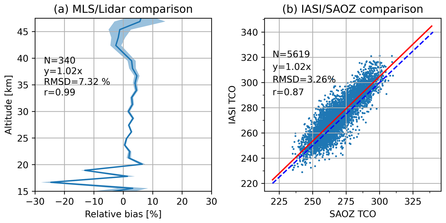
Figure 4 (a) Mean relative bias (solid line) and standard error (shaded area) computed from Eq. (1) comparing nocturnal DIAL ozone profiles to the corresponding daily MLS v5 ozone profiles between January 2013 and December 2021. (b) Direct comparison between SAOZ total column ozone (TCO) and IASI TCO from data points obtained between March 2013 and December 2021. The solid red and dashed blue lines represent the linear regression line and the 1:1 line, respectively. Statistical results presented on the left side each of panel were obtained from the comparison of all data points, irrespective of the altitude level, date, and time of day.

Concerning ozone profiles, the best agreement is found in the 20–40 km altitude range, with larger biases and increasing deviations below 20 km and above 40 km. In the altitude range from 20 to 40 km, MLS has a relative bias and error (i.e., relative bias and error averaged over the 20–40 km altitude range, with respect to DIAL measurements) of 2.76±0.70 %. In this altitude range, the standard error is low because of the large number of available comparison profiles (up to a maximum of 340). Between 40 and 45 km, the average relative bias decreases slightly in magnitude but changes sign ($-\mathrm{1.32}\pm \mathrm{2.40}$ %), whereas below 20 km it shows an average of $-\mathrm{6.04}\pm \mathrm{3.77}$ %. The increased relative bias and standard error at altitudes greater than 40 km is partly due to the lidar SNR decrease and the reduced number of lidar profiles reaching altitudes greater than 45 km. The decrease in SNR requires additional signal filtering, which introduces a high bias in the ozone lidar profile with respect to other measurements (Godin et al., 1999). Consequently, the lidar mean measurement error increases from ∼10 % at 40 km to ∼50 % at 47.5 km. Additionally, out of the 470 lidar profiles, 410 reached 40 km, 132 reached 45 km, and only 6 reached 47.5 km. Note also that the increased relative bias and standard error below 20 km are mainly due to low ozone mixing ratios at these altitudes, and possibly to reduced satellite accuracy and precision (see Table 3.18.1 of Livesey et al., 2022), as well as a smaller number of lidar profiles in this region. Indeed, out of the 470 profiles, only 453 extend below 20 km, 409 below 17.5 km, and 131 below 15 km. Over the whole altitude range, the correlation coefficient (r=0.99) indicates an excellent correlation between the lidar and MLS, while the linear regression (y=1.02x) and the mean relative bias profile show that MLS profiles tend to slightly over-estimate ozone concentrations relative to DIAL, in the 20–40 km range. Finally, a moderate relative deviation (RMSD =7.32 %) further demonstrates the agreement between MLS and the DIAL profiles.

Concerning TCO data, the large number of comparison points (N=5619) enables precise statistics, indicating low relative deviation (RMSD =3.26 %) and a fairly strong correlation (r=0.87) between IASI and SAOZ datasets. The linear regression (y=1.02x) shows that IASI TCO tends to slightly over-estimate SAOZ TCO.

Therefore, as expected, the MLS ozone profiles are in good agreement with lidar observations in the 20–40 km altitude range, including the altitudes of the Hunga-affected layers (25–30 km) that are our main focus in this study. The IASI and SAOZ TCO also exhibit low relative deviation and a high degree of correlation throughout the comparison period.

3.4 Effects of the volcanic plume on ozone

Based on the excellent correlation and agreement between satellite (MLS and IASI) and ground-based (stratospheric lidar and SAOZ) instruments over Réunion, we now use satellite ozone products to investigate the changes in the distribution of ozone over the study region.

Figure 5 depicts daily spatial distributions of SCO (panels a1–a9), SCO anomalies (panels b1–b9), and total SO₂ (panels c1–c9) over the Indian Ocean from 15 to 23 January. Similarly, Fig. A1 in Appendix A provides the corresponding spatial distributions for TCO. Anomaly and SO₂ spatial distributions are overlaid with red contours of the SO₂ plume, indicating regions where the SO₂ total column is greater than 30 DU. SO₂ spatial distributions are complemented by the MLS satellite track (blue circles), with the MLS profiles meeting the Hunga-influenced selection criterion marked by dark blue circles. As described in Sect. 2.1.3, this selection criterion retains profiles if the v4 MLS H₂O mixing ratio exceeds 100 ppmv within the 10–100 hPa layer and if the maximum occurs specifically at either 26.10 hPa (∼25 km) or 14.68 hPa (∼28 km), corresponding to the two Hunga-influenced layers. The successive locations of the SO₂ plume and the Hunga-influenced MLS profiles, which capture the H₂O and ozone anomalies, show the east-to-west displacement of Hunga-influenced air masses reported by previous studies (e.g., Millán et al., 2022; Khaykin et al., 2022; Baron et al., 2023). The simultaneous displacement of the SO₂ and H₂O plumes supports previous studies, and the rapid disappearance of the high SO₂ anomaly indicates its conversion into sulfates under the influence of excess H₂O (Legras et al., 2022; Zhu et al., 2022, 2023; Asher et al., 2023).

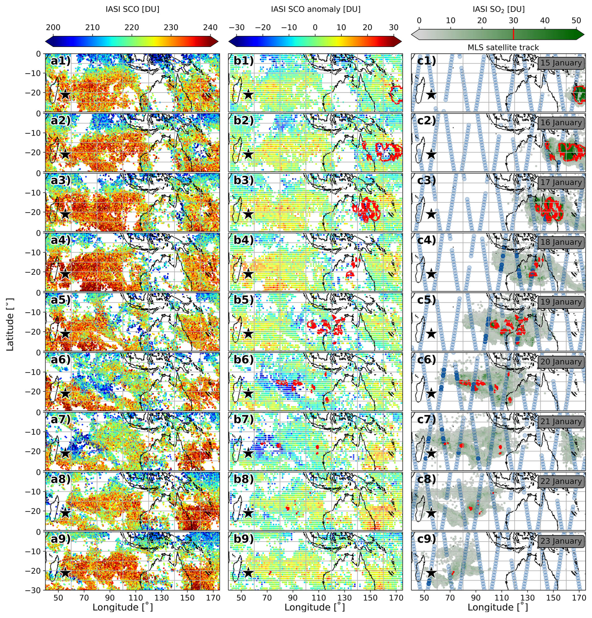
Figure 5 Daily evolution of (a1–a9) stratospheric column ozone (SCO) and (b1–b9) SCO anomaly observed by IASI alongside (c1–c9) the satellite track of MLS (blue dots) and total SO₂ column from IASI between 15 and 23 January 2022. Dark blue dots on the MLS track represent the location of profiles meeting the Hunga-influenced selection criterion. The red contour indicates the regions where total SO₂ column is greater than 30 DU. The black and white star represents the location of Réunion. Each row represents a different day, with the observation date shown in the rightmost column.

This zonal movement is also reflected in the daily spatial distributions and anomalies of IASI TCO and SCO, suggesting a correlation between ozone, H₂O, and SO₂ anomalies. The first significant negative ozone anomaly linked to Hunga appears on 15 January at 171° E, with values of $-\mathrm{5.3}\pm \mathrm{4.7}$ DU for TCO and $-\mathrm{16.4}\pm \mathrm{4.7}$ DU for SCO, where the uncertainty accounts for both the anomaly and column values from daily IASI observations. On this date, the fifth percentile of the anomaly is −10.0 DU for TCO and −6.2 DU for SCO. This first ozone anomaly is attributed to the lofting of ozone-poor tropospheric air masses (Zhu et al., 2023; Evan et al., 2023). The anomaly then appears to grow larger in size and amplitude as the SO₂ plume spreads, despite cloudy conditions on 18 January hindering IASI observations, before reaching Réunion on 21 January. The rapid conversion of SO₂ molecules to sulfate particles in the first days following the eruption increased the aerosol surface area, resulting in ozone depletion through heterogeneous chemistry (Zhu et al., 2023; Evan et al., 2023).

IASI recorded the highest number of negative ozone anomalies linked to Hunga on 20 and 21 January (panels a6–a7 and b6–b7 of Figs. 5 and A1). On 21 January, the fifth percentile of the anomaly peaked at −18.6 DU for TCO and at −14.5 DU for SCO. On the same day, extreme anomalies of $-\mathrm{19.3}\pm \mathrm{5.0}$ DU for TCO and $-\mathrm{32.8}\pm \mathrm{4.9}$ DU for SCO were observed at 71° E. At the same location, the IASI average SCO is 233.9±9.4 DU, meaning this anomaly is more than three times larger than the typical variation. For TCO, the anomaly is about twice the climatological variability based on SAOZ data (262.8±11.9 DU) and three times the variability derived from IASI's mean (258.9±6.2 DU). The IASI anomaly spatial distributions for 20 and 21 January suggest the appearance of a large transient ozone depletion event extending over approximately 30° of longitude and 20° of latitude. The presence of clouds on 22 January hindered the retrieval of IASI data between Réunion and Madagascar, but large anomalies were still visible in the region on 23 January. The ozone anomaly then exited the Indian Ocean (not shown). Therefore, the anomaly spatial distributions and MLS satellite track indicate that the study region was subject to TCO, SCO, and H₂O anomalies over the latitudinal band from 30° to 10° S, with a zonal westward shift of the ozone minimum. Similar to the findings of Evan et al. (2023), our results indicate the colocation of the H₂O and ozone anomalies as the Hunga plume passed over the Indian Ocean.

MLS profiles identified by the criterion were studied further. Hunga-influenced profiles, defined as those with a water vapor mixing ratio exceeding 100 ppmv between 10 and 100 hPa, are categorized into two groups: those influenced by the higher-altitude plume, with the highest water vapor mixing ratio at 14.68 hPa, and those influenced by the lower-altitude plume, with the maximum mixing ratio at 26.10 hPa. For each group of Hunga-influenced H₂O and ozone profiles, we computed the difference from their corresponding background average profiles. Subsequently, these individual differences were averaged, and results are presented in Fig. 6a and b, where the horizontal bars represent the ±1σ standard deviation around the mean value. Panels c and d present the same data on an altitude grid, with ozone anomaly profiles converted to partial columns using geopotential and temperature information.

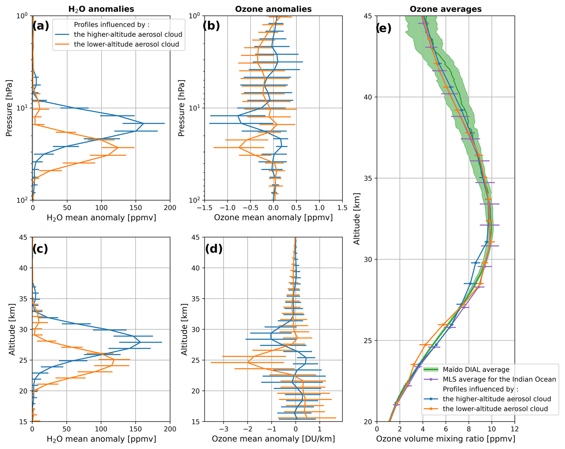
Figure 6 Mean anomalies and ±1σ standard deviation (horizontal bars) in (a–c) water vapor and (b–d) ozone from v4 MLS profiles that met the selection criterion. (a–b) present measurements from raw profiles in volume mixing ratio over a pressure range, while (c–d) show the same data over an altitude range, with ozone expressed in DU km⁻¹. (e) displays the January mean lidar ozone profile with its ±2σ standard deviation, the MLS average ozone profile for the Indian Ocean with its ±1σ standard deviation, and the average v4 MLS ozone profiles influenced by the Hunga clouds with the corresponding ±1σ standard deviation. Profiles influenced by the higher-altitude and lower-altitude clouds are displayed in blue and orange, respectively.

The ozone mean anomaly associated with the higher-altitude cloud is (1σ) significant at the 12.11 hPa level and barely (1σ) significant at the 14.68 hPa pressure level, with an average anomaly of $-\mathrm{0.7}\pm \mathrm{0.6}$ ppmv ($-\mathrm{1.0}\pm \mathrm{1.0}$ DU km⁻¹) across these two pressure levels. In percentage terms, this corresponds to $-\mathrm{5.5}\pm \mathrm{4.7}$ % and $-\mathrm{6.3}\pm \mathrm{4.8}$ % with respect to the average MLS profile over the Indian Ocean (Fig. 6e, purple line) and the mean lidar profile (Fig. 6e, green line), respectively. For the lower-altitude cloud, (1σ) significant ozone anomalies occur across the 21.54–31.62 hPa pressure range, with a mean anomaly of $-\mathrm{0.6}\pm \mathrm{0.5}$ ppmv ($-\mathrm{1.7}\pm \mathrm{1.4}$ DU km⁻¹), corresponding to $-\mathrm{7.5}\pm \mathrm{7.0}$ % and $-\mathrm{8.5}\pm \mathrm{8.1}$ % with respect to the mean MLS Indian Ocean and the mean lidar profiles, respectively. These results are consistent with those of Evan et al. (2023), who documented a 5 % depletion of stratospheric ozone over the Indian Ocean.

While Figs. 5 and A1 revealed local SCO and TCO minima, Fig. 6 shows clear reduction in stratospheric ozone (in the range 30–12 hPa, corresponding to 23.5–30.0 km) linked to sulfate aerosols and excess water vapor. This observation confirms previous research (Evan et al., 2023; Zhu et al., 2023) and indicates that the ozone anomaly arose from chemical loss.

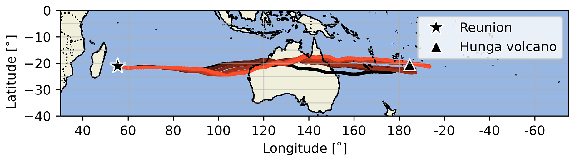
Figure 7 HYSPLIT back trajectories of 240 h ending on 21 January at 00:00 UTC at the location of Saint-Denis, Réunion, between 23.5 and 29.0 km height. The star and triangle symbols indicate the ending point and the Hunga volcano location, respectively. The back trajectories are displayed with a color gradient, ranging from black for the trajectory ending at 23.5 km to orange for 29.0 km.

3.5 Transport of air masses in the stratosphere

The Lagrangian HYSPLIT model was used to investigate the origin of the air masses responsible for the ozone anomaly over the Indian Ocean following the Hunga eruption. Back trajectories were run from the location of Réunion on 21 January at 00:00 UTC for 12 distinct altitudes ranging between 23.5 and 29.0 km. Figure 7 shows the result of the HYSPLIT simulation with a color gradient to distinguish different air parcels. The orange trajectory represents air masses at 29.0 km altitude, and the black trajectory represents air masses at 23.5 km. Figure 7 shows that all back trajectories are zonal, moving westward and passing over the location of the Hunga eruption. The results of the HYSPLIT back trajectory simulation are consistent with the lidar measurements made in Réunion (see Fig. 2), as well as with the ozone anomalies over the region of study as depicted in Figs. A1 and 5. Additionally, these two figures show a westward transition of ozone anomalies in the stratosphere over the Indian Ocean. The results of this trajectory simulation provide further confirmation of the Hunga plume's passage over Réunion, as previously established by Baron et al. (2023) and Evan et al. (2023).

4 Conclusions

The main eruption of the Hunga volcano released significant amounts of water vapor and a moderate quantity of sulfur dioxide into the atmosphere (Sellitto et al., 2022; Zuo et al., 2022; Millán et al., 2022), resulting in substantial anomalies within the stratosphere. Here we use satellite observations from IASI, MLS, and OMPS, complemented by ground-based measurements from Réunion, to provide a detailed view of the evolution of colocated ozone, water vapor, and SO₂ anomalies in the early volcanic plume over the Indian Ocean. This study presents the first analysis of IASI data in the context of Hunga.

OMPS aerosol extinction profiles revealed that the volcanic plume extended through the stratosphere, from 5° to 25° S, and reached altitudes greater than 35 km over the Indian Ocean. These results are supported by the Maïdo aerosol lidar, which observed the plume during two consecutive nights, indicating that the core of the plume passed over Réunion at an altitude ranging from 26.8 to 29.7 km. Lidar sAOD and sun-photometer total AOD recorded unprecedented values of 0.84±0.27 and 0.57±0.04, respectively, during the passage of the plume.

The ozone anomaly associated with the volcanic plume was investigated using MLS and IASI ozone data. Based on these results, we state that the advection of the volcanic aerosol and water vapor plumes had an impact on stratospheric and total ozone abundances over the Indian Ocean. As indicated by IASI, a transient ozone depletion event was observed over the region, with the fifth percentile of the anomaly reaching −18.6 DU for total column ozone (TCO) and −14.5 DU for stratospheric column ozone (SCO) on 21 January. On the same day, extreme anomalies of $-\mathrm{19.3}\pm \mathrm{5.0}$ DU for TCO and $-\mathrm{32.8}\pm \mathrm{4.9}$ DU for SCO were observed, significantly exceeding climatological variability. Hunga-influenced MLS profiles show a significant reduction in ozone over the 30–12 hPa pressure range.

Ozone depletion occurred in two distinct layers, associated with two separate sulfate aerosol clouds with excess water vapor. Within the higher-altitude (14.68–12.12 hPa) cloud, ozone decreased by an average of 0.7±0.6 ppmv (1.0±1.0 DU km⁻¹). In percentage terms, this corresponds to $-\mathrm{5.5}\pm \mathrm{4.7}$ % with respect to the average MLS profile over the Indian Ocean. Within the lower-altitude (31.62–21.54 hPa) cloud, ozone decreased by an average of 0.6±0.5 ppmv (1.7±1.4 DU km⁻¹), corresponding to $-\mathrm{7.5}\pm \mathrm{7.0}$ % with respect to the mean MLS Indian Ocean profile. Our findings refine previous reports of chemical ozone loss in the week following the eruption by showing that it was confined to two distinct aerosol layers with excess H₂O. This structured depletion offers new insight into the influence of Hunga aerosol distribution on ozone loss.

Appendix A

This section presents daily spatial distributions of TCO (Fig. A1a1–a9), TCO anomalies (Fig. A1b1–b9), and total SO₂ (Fig. A1c1–c9) over the Indian Ocean from 15 to 23 January.

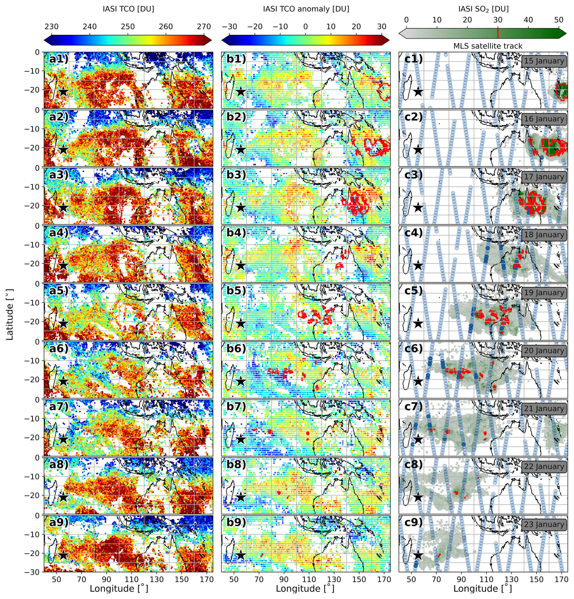
Figure A1 Daily evolution of (a1–a9) total column ozone (TCO) and (b1–b9) TCO anomaly observed by IASI alongside (c1–c9) the satellite track of MLS (blue dots) and total SO₂ column from IASI between 15 and 23 January 2022. Dark blue dots on the MLS track represent the location of profiles meeting the Hunga-influenced selection criterion. The red contour indicates the regions where the total SO₂ column is greater than 30 DU. The black and white star represents the location of Réunion. Each row represents a different day, with the observation date shown in the rightmost column.