Mid-Atlantic US observations of radiocarbon in CO₂: fossil and biogenic source partitioning and model evaluation

Accurately quantifying regional anthropogenic CO₂ fluxes is fundamental to improving our understanding of the carbon cycle and for creating effective carbon mitigation policies, and the radiocarbon to total carbon ratio in atmospheric CO₂ (Δ¹⁴CO₂) is a robust tracer of fossil fuel CO₂ that can discriminate between biogenic and fossil fuel CO₂ sources. NASA's Atmospheric Carbon and Transport-America (ACT-America) airborne mission between 2016 and 2019 aimed to improve the accuracy of regional greenhouse gas flux estimates, through refining our understanding and characterization of fluxes and flux uncertainties in models. Δ¹⁴CO₂ observations from 26 flights are presented for examining seasonal CO₂ source partitioning in the Mid-Atlantic USA. Observed variability in boundary layer CO₂ at timescales ranging from intra-day to seasonal was largely driven by biogenic CO₂ (CO_2bio) variability that ranged from −19.7 ppm in summer to 16.2 ppm in fall, while fossil fuel CO₂ (CO_2ff) variability remained at 3.3±2.0 ppm. Carbonyl sulfide uptake was well-correlated with CO_2bio uptake, and examining this relationship, as well as that between CO₂ and CO_2bio variability reinforces the seasonal extent of gross primary productivity response throughout ACT-America. We use airborne Δ¹⁴CO₂ flask sampling alongside in situ carbon monoxide measurements to calculate high-frequency CO_2ff and evaluate the magnitude and diurnal variability of modeled CO_2ff, deducing likely transport errors in an example flight. Although ACT-America CO_2ff signals were attenuated due to the broad source regions sampled, results illustrate the value of Δ¹⁴CO₂ sampling and observation-based methodologies for regional CO₂ flux attribution, evaluation and improvement of modeled CO₂.

1 Introduction

Anthropogenic carbon dioxide (CO₂) emissions have driven more than a 50 % increase in atmospheric CO₂ abundances globally since pre-industrial levels, despite almost half of these emissions being removed from the atmosphere by terrestrial and oceanic reservoirs (i.e., “sinks”; Ballantyne et al., 2012; Friedlingstein et al., 2022). Because total CO₂ fluxes encompass biogenic, oceanic and anthropogenic processes and because regional spatial scales are ones at which carbon mitigation strategies are generally developed and implemented, it is important that these CO₂ component processes be accurately quantified. Fossil fuel emissions represent the bulk of the net atmospheric CO₂ flux annually on regional scales for North America (King et al., 2007; USGCRP, 2018). However, while national-scale fossil fuel CO₂ fluxes for many countries are likely known to within 10 % (Gregg et al., 2009; Andres et al., 2012), fluxes and their variability are less certain on smaller spatial and temporal scales (USGCRP, 2018; Gurney et al., 2021). Even so, fossil fuel fluxes are currently reported with uncertainties up to 5 times lower than biospheric CO₂ fluxes on regional scales (Hayes et al., 2012; King et al., 2015; USGCRP, 2018).

Atmospheric CO₂ and its long-term global growth rate can be directly determined from in situ observations, because observed CO₂ over large land areas is a function of both fossil fuel emissions and net ecosystem exchange (NEE) with the terrestrial biosphere. Distinguishing fossil fuel from biogenic CO₂ fluxes cannot be accomplished from CO₂ observations alone (Shiga et al., 2014; Basu et al., 2016). The radiocarbon to total carbon ratio in atmospheric CO₂ (¹⁴C : C, expressed as Δ¹⁴CO₂) has been demonstrated to be a robust and largely unbiased tracer for accurately constraining recently emitted fossil fuel CO₂ (CO_2ff) into the atmosphere because fossil fuels do not contain ¹⁴C (Levin et al., 2003; Levin and Karstens, 2007; Graven et al., 2009; Vogel et al., 2010; Miller et al., 2012; Turnbull et al., 2006, 2011a, b, 2015). By isolating this fossil fuel component and its variability relative to background levels, the remaining variability in CO₂ can be attributed to biogenic processes.

Inverse models using only CO₂ measurements can theoretically be used to disaggregate anthropogenic and biogenic CO₂ fluxes when these emissions can be adequately separated in time and space, but given the low density of most regional measurement networks, fossil and biogenic fluxes are colocated, so this disaggregation cannot be achieved in practice (Shiga et al., 2014; Basu et al., 2016). In many situations from regional to global scales, prior fossil CO₂ emissions are traditionally pre-specified and not optimized in CO₂ measurement-based inversions (Gurney et al., 2003; Ciais et al., 2010; Schuh et al., 2010; Lauvaux et al., 2012) on the basis that fossil fluxes are much better known than terrestrial biospheric fluxes. Much work has been done to characterize model uncertainty and improve estimates of CO₂. At the continental scale and for annual time frames, Feng et al. (2019a) used a forward-calibrated model ensemble (Feng et al., 2019b) to show that the uncertainty in simulated North American atmospheric CO₂ mole fractions comes primarily from two approximately equivalent sources: fossil fuel emissions and biogenic CO₂ fluxes. At these timescales, these two sources greatly outweighed the uncertainty contributions from atmospheric transport and from continental boundary conditions, and Feng et al. (2019a) note that accurate accounting of fossil fuel emissions uncertainties in models can further improve regional biospheric flux estimates. Brophy et al. (2019) emphasized the need for varying prior fossil fuel emissions estimates in time, alongside needed improvements in the representation of atmospheric transport to accurately represent CO₂ fluxes at approximately sub-annual and regional scales. Modelers have also relaxed the assumption of perfectly known fossil CO₂ emissions – and have lowered fossil fuel emissions uncertainties – by assimilating Δ¹⁴CO₂ measurements (or CO_2ff) alongside CO₂ and carefully controlling systematic model errors and errors in prior flux estimates (Basu et al., 2016, 2020; Fischer et al., 2017).

Using aircraft Δ¹⁴CO₂ observations, an effort has been made to evaluate modeled CO_2ff and to estimate or verify regional emissions inventories (e.g., Graven et al., 2009; Basu et al., 2020). At the urban scale, studies have also successfully used Δ¹⁴CO₂ measurements alongside in situ carbon monoxide (CO) observations from surface- and aircraft-based platforms to calculate high-resolution proxy estimates of recently added CO_2ff to the atmosphere, given well-characterized CO : CO_2ff ratios (Vogel et al., 2010; Turnbull et al., 2011a, 2019; Lauvaux et al., 2020; Wu et al., 2022). As biogenic CO₂ emissions and sinks – even within cities – are non-negligible and as ignoring these signals could potentially bias fossil fuel CO₂ emissions inventories, Δ¹⁴CO₂ measurements play an important role in determining biogenically driven (CO₂ photosynthesis and respiration) emissions or sinks (Levin et al., 2003; Lopez et al., 2013; Turnbull et al., 2015; Miller et al., 2020). One tracer that could aid in the understanding of CO₂ uptake processes alongside Δ¹⁴CO₂ is carbonyl sulfide (OCS), which is taken up by plants but not respired (Montzka et al., 2007; Campbell et al., 2008).

NASA's multi-year Atmospheric Carbon and Transport (ACT)-America Earth Venture Suborbital mission was directed toward improving the accuracy of regional greenhouse gas flux estimates, specifically through refining our understanding and implementation of CO₂ and methane (CH₄) transport, fluxes and flux uncertainties, and background levels in inverse models (Davis et al., 2021). During this mission, five seasonal research flight campaigns were conducted between 2016 and 2019 for evaluation and subsequent improvement of terrestrial carbon cycle models and for filling gaps in the eastern US carbon monitoring network. With a strong focus on transport of carbon via weather systems, atmospheric trace gases and meteorological variables were also observed across multiple synoptic cycles, across cold and warm air sectors, and from the boundary layer to the upper troposphere. While the ACT mission was not targeting large carbon emissions signals in urban areas as in the abovementioned studies, we focus on carbon flux attribution and model evaluation here. We analyze a spatially dense set of airborne whole-air flask Δ¹⁴CO₂ measurements collected during ACT in the Mid-Atlantic USA alongside those of other gas-phase species such as OCS, a tracer for photosynthetic uptake of CO₂, to first distinguish between biogenically driven and fossil fuel atmospheric CO₂ variability relative to background levels. Second, we apply the methodology of previous authors (Levin and Karstens, 2007; Vogel et al., 2010; Turnbull et al., 2011a; Maier et al., 2024a) to the broad Mid-Atlantic US region, calculating high-frequency fossil fuel CO₂ enhancements using in situ CO observations, and we investigate the utility of this technique for evaluating modeled atmospheric fossil fuel CO₂ enhancements above background levels for an example ACT research flight along the northeastern corridor.

2 Data and methods

2.1 ACT-America flight campaigns

During the ACT mission, the eastern half of the coterminous USA was broadly surveyed by two research aircraft: the NASA Langley Beechcraft B-200 King Air and the NASA Wallops C-130 Hercules. Of the Mid-Atlantic, Midwestern and Southern US-focused measurement regions, air samples for Δ¹⁴CO₂ measurement were collected only in the Mid-Atlantic region due to proximity to the northeastern US urban corridor and likelihood for higher Δ¹⁴CO₂ signals. Sampling in the Mid-Atlantic region focused heavily on the extensive forests and croplands with flights capturing distant urban influence, and a few selected flights specifically targeted the urban northeastern corridor. The first ACT campaign occurred during summer 2016 (18 July–28 August) and is omitted from this analysis due to the absence of Δ¹⁴CO₂ sampling. Four subsequent ACT campaigns described here occurred during winter 2017 (1–10 March), fall 2017 (1–15 October), spring 2018 (4–20 May) and summer 2019 (7–27 July) for a total of 26 flights with atmospheric sampling for Δ¹⁴CO₂. Research flights were primarily conducted between 11:00 and 18:00 LT (local time) to sample a well-developed atmospheric boundary layer (ABL), through long, level-leg flight transects. Airborne atmospheric sampling during individual research flights was focused at altitudes within the ABL (flight altitudes of 330 m a.g.l. (above ground level) in most cases) where greenhouse gas abundances are strongly influenced by surface fluxes with occasional sampling in the free troposphere (FT, ∼2400 to 9000 m a.m.s.l. (above mean sea level)) to determine chemistry and isotopic composition of background air against which observed ABL enhancements or depletions are assumed to occur. Because a scientific goal of ACT was to improve the simulation of atmospheric transport of greenhouse gases in regional-scale inversions under real-world conditions, research flights were organized to sample across synoptic weather patterns (Pal et al., 2020). Wei et al. (2021) describe the ACT observational and numerical data products.

2.2 Whole-air sample collection and flask radiocarbon measurements

NOAA Programmable Flask Packages (PFPs) were installed on each aircraft for the collection of whole-air samples. Each PFP contains twelve 0.7 L borosilicate glass flasks, and for ACT campaigns between 2017 and 2019 these automated systems were connected to a Peltier gas chiller to efficiently dry air samples to less than 1 % atmospheric water vapor prior to air sample collection. Flask-filling times varied between 2 (ABL) to 4 min (FT), depending on the altitude of the aircraft. A Programmable Compressor Package (PCP) pressurized each flask to 275 kPa, yielding ∼2 L of air at standard temperature and pressure conditions collected per flask. The technical details of these flask sampling systems used during ACT are described in Baier et al. (2020).

For each flight day, roughly 6 to 18 total flasks were filled on each aircraft platform between the altitudes of 300–9000 m a.m.s.l. The ratio of well-mixed ABL to FT flasks sampled during ACT was generally 5:1. Because approximately 2 L of sample air is required for high-precision Δ¹⁴CO₂, in addition to the long-lived greenhouse gases (CO₂, CH₄) and other low concentration gases such as OCS and CO, two PFP flasks were filled in parallel (i.e., “paired sampling”) when sampling for Δ¹⁴CO₂ measurements. Post-flight, PFPs were transferred to the NOAA Global Monitoring Laboratory and the University of Colorado INSTAAR Stable Isotope Laboratory for measurement. The first flask of each paired sample was analyzed for greenhouse gases; OCS; and a suite of hydrocarbons, halocarbons, and stable isotope ratios (¹³C : ¹²C) of CO₂ and methane using methods described in Baier et al. (2020), online (https://gml.noaa.gov/ccgg/aircraft/analysis.html, last access: 5 November 2024), and in Vaughn et al. (2004). Remaining sample air in the first flask after these measurements was combined with the entire second paired flask for a single Δ¹⁴CO₂ measurement. The University of Colorado INSTAAR Laboratory for AMS Radiocarbon Preparation and Research (NSRL) conducts the CO₂ extraction from flask sample air. Pure CO₂ is archived until near the time of Δ¹⁴CO₂ measurement, at which time the pure CO₂ is graphitized to pure carbon “targets”, and these graphitized samples are transferred to the University of California at Irvine for high-count accelerator mass spectrometry (AMS) ¹⁴C measurement (Turnbull et al., 2007; Lehman et al., 2013). In total, 380 ¹⁴CO₂ samples were analyzed throughout the ACT campaigns: 87 in winter 2017, 100 in fall 2017, 104 in spring 2018 and 89 in summer 2019.

2.3 Radiocarbon-based CO₂ partitioning

Radiocarbon (¹⁴C) is produced naturally in the troposphere and stratosphere via cosmic-ray-induced reactions between neutrons and atmospheric nitrogen (N₂) (Libby, 1946). Measurements are presented as Δ¹⁴CO₂ in units of per mill (‰), i.e., the part per thousand deviation of the measured ¹⁴C : C ratio from that of the international measurement standard material, after correction for mass-dependent fractionation and radioactive decay since the date of collection (Stuiver and Polach, 1977). Given that the ¹⁴C half-life is approximately 5730 years (Godwin, 1962) and that fossil fuel carbon has been isolated from the atmosphere for millions of years, the radiocarbon content of fossil fuels is zero; therefore, Δ¹⁴CO_2ff is −1000 ‰ on the delta (Δ) scale. Therefore, addition of fossil fuel CO₂ to the atmosphere produces a quantitative reduction in atmospheric Δ¹⁴CO₂ over and downwind of emissions sources. Paired observations of Δ¹⁴CO₂ and CO₂ in flasks sampled in the Mid-Atlantic region can thereby provide a robust method for distinguishing between terrestrial biogenic (CO_2bio) and fossil fuel (CO_2ff) CO₂ sources, given a known background. The CO₂ mass balance over land is

$$\begin{array}{}\text{(1)}& {\mathrm{CO}}_{\mathrm{2}\mathrm{obs}}={\mathrm{CO}}_{\mathrm{2}\mathrm{bg}}+{\mathrm{CO}}_{\mathrm{2}\mathrm{ff}}+{\mathrm{CO}}_{\mathrm{2}\mathrm{bio}}.\end{array}$$

Expanding CO_2bio, which results from net ecosystem exchange, into a sum of photosynthetic (photo) and respiration (resp) fluxes (CO_2resp+CO_2photo) and adding the respective isotopic signatures (“Δ”, for Δ¹⁴CO₂) for all terms gives Eq. (2):

$$\begin{array}{}\text{(2)}& \begin{array}{rl}{\mathrm{\Delta }}_{\mathrm{obs}}{\mathrm{CO}}_{\mathrm{2}\mathrm{obs}}& ={\mathrm{\Delta }}_{\mathrm{bg}}{\mathrm{CO}}_{\mathrm{2}\mathrm{bg}}+{\mathrm{\Delta }}_{\mathrm{ff}}{\mathrm{CO}}_{\mathrm{2}\mathrm{ff}}+{\mathrm{\Delta }}_{\mathrm{resp}}{\mathrm{CO}}_{\mathrm{2}\mathrm{resp}}\\ & +{\mathrm{\Delta }}_{\mathrm{photo}}{\mathrm{CO}}_{\mathrm{2}\mathrm{photo}}+{\mathrm{N}}^{\mathrm{14}}{C}_{\mathrm{nuc}}/R_{\mathrm{std}},\end{array}\end{array}$$

where the individual budget terms are the product of the isotopic ratio and CO₂ mole fraction, which is a conserved quantity (Tans et al., 1993). Here, “obs” is the observed atmospheric mole fraction of CO₂ in the ABL and is a function of variations in fossil fuel (ff) and biogenic (bio) CO₂ differences from a varying CO₂ background (bg) level. We note that an oceanic term is sometimes written in Eq. (1), but we assume that the dominant oceanic CO₂ influence is encompassed in the background (bg) term. Photosynthesis and respiration contributions are stated separately in the isotopic mass balance (Eq. 2), because they carry different isotopic signatures. This isotopic “disequilibrium” between photosynthetic and respiration fluxes arises from the rapidly decreasing ($\sim -\mathrm{5}$ ‰ yr⁻¹) background Δ¹⁴CO₂ (e.g., Lehman et al., 2013; Graven et al., 2020). Δ_resp is more positive than Δ_photo, because Δ_resp is associated with biospheric CO₂ fixed by photosynthesis when the ambient atmospheric Δ¹⁴CO₂ (i.e., Δ_bg) was higher. Δ_photo is assumed equal to Δ_bg, because the “Δ” notation accounts for mass-dependent fractionation processes such as those occurring during photosynthesis. Turnbull et al. (2009) note that this assumption is valid in the limit that time and space between background and observation tends to zero. There is also a small impact on Δ_obs from pure ¹⁴C emitted from certain nuclear reactors, which is added as the last term in Eq. (2) (Graven and Gruber, 2011). Because this term is significantly smaller than all other terms in Eq. (1), it is omitted there. Here N is the mass-dependent Δ normalization factor, which is close to 1 (Basu et al., 2016), ¹⁴C_nuc is the mole fraction of Δ¹⁴CO₂ resulting from the ¹⁴C flux from reactors, and R_std is the standard material ¹⁴C $/$ C ratio.

Combining Eqs. (1) and (2) results in

$$\begin{array}{}\text{(3)}& \begin{array}{rl}{\mathrm{CO}}_{\mathrm{2}\mathrm{ff}}& ={\displaystyle \frac{{\mathrm{CO}}_{\mathrm{2}\mathrm{obs}}\left({\mathrm{\Delta }}_{\mathrm{obs}}-{\mathrm{\Delta }}_{\mathrm{bg}}\right)}{\left({\mathrm{\Delta }}_{\mathrm{ff}}-{\mathrm{\Delta }}_{\mathrm{bg}}\right)}}-{\displaystyle \frac{{\mathrm{CO}}_{\mathrm{2}\mathrm{resp}}\left({\mathrm{\Delta }}_{\mathrm{resp}}-{\mathrm{\Delta }}_{\mathrm{bg}}\right)}{\left({\mathrm{\Delta }}_{\mathrm{ff}}-{\mathrm{\Delta }}_{\mathrm{bg}}\right)}}\\ & -{\mathrm{N}}^{\mathrm{14}}{C}_{\mathrm{nuc}}/R_{\mathrm{std}}/\left({\mathrm{\Delta }}_{\mathrm{ff}}-{\mathrm{\Delta }}_{\mathrm{bg}}\right).\end{array}\end{array}$$

The variables in Eq. (3) are either known or can be measured or calculated directly. Historically, CO_2ff has been approximated by only the first term on the right-hand side of Eq. (3) (Levin et al., 2003). Disequilibrium and nuclear fluxes both add ¹⁴C to the atmosphere. A correction (CO_2corr) is made to CO_2ff (Turnbull et al., 2009) to unmask these effects and reveal the full magnitude of the fossil fuel CO₂ emissions signal, making it somewhat convenient to rewrite Eq. (3) as

$$\begin{array}{}\text{(4)}& {\mathrm{CO}}_{\mathrm{2}\mathrm{ff}}={\displaystyle \frac{{\mathrm{CO}}_{\mathrm{2}\mathrm{obs}}\left({\mathrm{\Delta }}_{\mathrm{obs}}-{\mathrm{\Delta }}_{\mathrm{bg}}\right)}{\left({\mathrm{\Delta }}_{\mathrm{ff}}-{\mathrm{\Delta }}_{\mathrm{bg}}\right)}}-{\mathrm{CO}}_{\mathrm{2}\mathrm{corr}}.\end{array}$$

Flask ABL measurements for CO_2obs are defined as those samples collected at altitudes less than 1500 m a.m.s.l. for all ACT flight campaigns. ABL samples typically contain the strongest regional flux signatures; thus, are likely to yield the largest Δ¹⁴C signals. Conversely, we determine daily Δ_bg and CO_2bg values from measurements of ¹⁴CO₂ and CO₂ in flasks sampled at altitudes greater than 4000 m a.m.s.l. for all flight campaigns to capture air that is within the well-mixed FT in all seasons. The FT data, while perhaps not always representative of the true local-scale background signature (e.g., Turnbull et al., 2015), are expected to provide a reliable estimate of the regional- to continental-scale background (Baier et al., 2020). Here, Δ_bg in Eq. (2) is derived as the daily mean FT Δ¹⁴CO₂, typically between 4000 and 9000 m a.m.s.l. All flask FT measurements are filtered to remove samples with high CO (above 3 standard deviations from a smooth curve fit), which can indicate the potential influence of local pollution on continental background values. Similarly, CO_2bg and other trace gas background mole fractions were derived as mean mole fractions of FT values for these species. For the ACT study, CO_2corr is derived for each flask sample by convolving estimated gridded monthly disequilibrium fluxes of Δ¹⁴CO₂ from the terrestrial biosphere and fluxes from nuclear reactors with surface influence functions for each flask sample location (i.e., for each flask “receptor”, as per below).

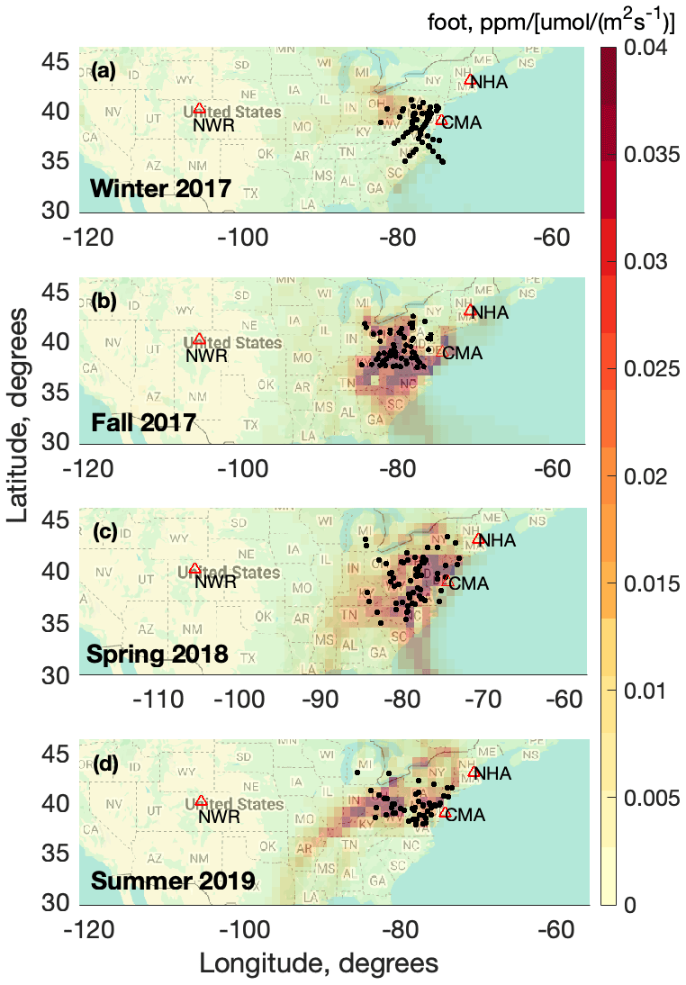
Figure 1 Surface influence for ABL Δ¹⁴CO₂ samples measured for ACT seasonal deployments in (a) winter 2017, (b) fall 2017, (c) spring 2018 and (d) summer 2019. ABL flask sample locations are denoted in black, with GGGRN aircraft program network sites indicated at Niwot Ridge, CO (NWR); Cape May, NJ (CMA); and Portsmouth, NH (NHA). Plot maps are produced using Google Maps API (© Google Maps 2025).

Surface influence functions (referred to as “footprints”), representing the sensitivity of air parcels at a particular receptor location to upwind surface fluxes (in units of ppm m² s µmol⁻¹), are derived by first using the HYbrid Single-Particle Lagrangian Integrated Trajectory (HYSPLIT) model (Stein et al., 2015), running 500 randomly perturbed, 10 d back-trajectories for all ABL flask receptors. Back-trajectories are driven by 27 km horizontal resolution Weather Research and Forecasting (WRF) meteorological fields, nudged to the ERA-5 reanalysis meteorology within the ACT-America North American model domain (Feng at al., 2021b; see Sect. 2.4). Individual footprints are calculated for all 500-particle trajectory ensemble members based on their residence time over a given gridded area (Lin et al., 2003) within the surface boundary, defined as a vertical column of air in each 1°×1° grid cell between 125 m a.g.l. and 50 % of the WRF-calculated atmospheric boundary layer height (Fig. 1). Referring to Eqs. (1) and (2), though there exists a footprint signature on flask samples during fall 2017 and spring 2018, this influence is relatively small. Disequilibrium fluxes from the terrestrial biosphere are derived by convolving impulse-response functions from the CASA biogeochemical model (Thompson and Randerson, 1999) with the atmospheric history of ¹⁴C (Miller et al., 2012; LaFranchi et al., 2013; with updates in Zhou et al., 2020), while nuclear reactor fluxes are obtained from Graven and Gruber (2011), effectively assuming regional nuclear ¹⁴CO₂ has not changed significantly over time through 2019. These gridded fluxes (monthly, time-dependent in the case of disequilibrium flux) are converted to the two components of CO_2corr via convolution with footprints derived from HYSPLIT and are calculated individually for each ABL flask sample pair for which CO_2ff is derived using Eq. (4). We note that the calculated magnitude of CO_2corr attributable to nuclear reactor emissions in the Mid-Atlantic USA is 0.25±0.44 ppm CO₂ and does not exhibit a seasonal pattern as it is assumed constant annually. Graven and Gruber (2011) data have been used at the time that this publication was written, but updates to nuclear reactor fluxes have been published in Zazzeri et al. (2023). The magnitude of CO_2corr attributable to the terrestrial biosphere in the Mid-Atlantic USA is approximately 0.10±0.04 ppm CO_2ff (1σ) during the winter deployment and exhibits a seasonal cycle with a maximum during the summer of 0.70±0.28 ppm CO_2ff (1σ), indicating similar seasonal behavior as that calculated by Miller et al. (2012) for the Mid-Atlantic USA. In total, the average magnitude of CO_2corr (0.8±0.6 ppm) calculated here to correct CO_2ff in this work is roughly comparable that first described in Turnbull et al. (2006).

2.4 Forward model CO_2ff using the PSUWRF model

A separate Eulerian 27 km horizontal resolution implementation of WRF-Chem version 3.6.1 run (Feng et al., 2021a, b) was implemented by The Pennsylvania State University (hereby called PSUWRF) with 50 vertical levels from the surface to 50 hPa, with 29 of these vertical levels in the lowermost 2 km. PSUWRF was developed and implemented during the ACT time period (2016–2019) to simulate atmospheric transport of CO₂ component fluxes along all flight tracks for each seasonal campaign. Note that while the Lagrangian HYSPLIT model mentioned above to calculate CO_2corr in Eq. (4) for each flask measurement also used WRF for input meteorological fields, this was not identical to PSUWRF that was used for the Eulerian simulations. PSUWRF model runs were implemented prior to this paper development and could not be rerun, but both WRF versions used similar setups; thus, we expect there to be no major inconsistencies between the use of these two different versions for calculating CO_2ff using flask or model output.

PSUWRF separately simulates the contributions of CO₂ boundary conditions and biogenic, ocean, fossil fuel, and biomass burning CO₂ fluxes to total CO₂ at any time and location in the model domain (Feng et al., 2019a, b). The microphysics, planetary boundary layer and cumulus parameterization schemes used in this run are Thompson microphysics, the Mellor-Yamada-Nakanishi-Nino version 2 (MYNN2) and the Kain–Fritsch schemes, respectively (Feng et al., 2019a). As the ACT campaigns spanned multiple years, CO₂ oceanic, fossil fuel and biomass burning fluxes, as well as total CO₂ boundary conditions, come from CarbonTracker version 2017 (CT2017) through 2017 and CT-NRTv2019-2 (Jacobson et al., 2020) afterwards. CT2017 and CT-NRTv2019-2 together are called “CT” for simplicity. The CT fossil fuel tracer typically is derived from an average of the ODIAC (Oda et al., 2018) and Miller emissions datasets. As both datasets have very similar global and national fossil fuel emissions totals but include differences in spatial and temporal emissions distributions, an average of the two is used in CT to optimize the mapping of these emissions (Jacobson et al., 2020). In PSUWRF, ODIAC and Miller datasets were run separately for initial model runs between 2016–2018 to experimentally investigate potential differences between the two; however, only small differences within ∼2 ppm CO_2ff are seen between the two and are not expected to create inconsistencies in CO_2ff simulated by PSUWRF between 2016–2019. As such, ODIAC and Miller are averaged to create a single flux product and to simplify model runs as in CT for 2019. In PSUWRF, simulated fossil fuel CO₂ (CO_2ffmod) is calculated using the same approach as flask CO_2ff, where average FT values of this tracer are subtracted from ABL values. The PSUWRF model transport is nudged to ERA5 reanalysis data to improve the depiction of atmospheric transport relative to ACT in-flight meteorological observations (Gerken et al., 2021). The PSUWRF model output was extracted to ACT research flight track locations at hourly resolution for comparison and evaluation relative to high-frequency measurement-based CO_2ff described in Sect. 2.5.

2.5 Calculation of “pseudo-CO_2ff”

As in previous studies (Levin and Karstens, 2007; Vogel et al., 2010; Turnbull et al., 2011a, Maier et al., 2024a), we employ in situ CO measurements for estimating CO_2ff (referred to as “pseudo-CO_2ff” and denoted as CO${}_{\mathrm{2}\mathrm{ff}}^{\prime }$) at high temporal resolution. ACT in situ CO measurements were made by cavity ring-down spectroscopy at 0.4 Hz, drift-corrected during flight and calibrated once weekly using gas standards on the World Meteorological Organization (WMO) X2014A CO scale, same as NOAA flask-based measurements (Wei et al., 2021; DiGangi et al., 2021). After calibration, CO data were averaged to 0.2 Hz, i.e., the maximum frequency of CO${}_{\mathrm{2}\mathrm{ff}}^{\prime }$. We calculate CO${}_{\mathrm{2}\mathrm{ff}}^{\prime }$ using Eq. (5) by applying a median ratio of CO to CO_2ff (R_CO) calculated strictly from flask samples collected each day (typically from 5–12 flask samples), and we apply this value to the in situ CO time series collected on that day's ACT research flight:

$$\begin{array}{}\text{(5)}& {\mathrm{CO}}_{\mathrm{2}\mathrm{ff}}^{\prime }={\displaystyle \frac{{\mathrm{CO}}_{\mathrm{obs}}^{\prime }-\stackrel{\mathrm{‾}}{{\mathrm{CO}}_{\mathrm{bg}}^{\prime }}}{R_{\mathrm{CO}}}}.\end{array}$$

Here, CO${}_{\mathrm{obs}}^{\prime }$ represents 0.2 Hz ABL (below 1500 m a.m.s.l.) in situ CO dry mole fraction observations, and $\stackrel{\mathrm{‾}}{{\mathrm{CO}}_{\mathrm{bg}}^{\prime }}$ represents the mean daily CO mole fraction observed in the FT (above 4000 m a.m.s.l.) for each flight day. R_CO is calculated as the median value of all flask measurements each day, i:

$$\begin{array}{}\text{(6)}& R_{\mathrm{CO}}={\displaystyle \frac{{\left[{\mathrm{CO}}_{\mathrm{obs},\mathrm{flask}}-\stackrel{\mathrm{‾}}{{\mathrm{CO}}_{\mathrm{bg},\mathrm{flask}}}\right]}_i}{{\mathrm{CO}}_{\mathrm{2}\mathrm{ff},\mathrm{flask}\mathrm{\_}\mathrm{i}}}}.\end{array}$$

A median R_CO is used each day due to difficulty with respect to calculating seasonal regression slopes with low correlations (seasonal R² between 0.08–0.33) in the flask CO enhancement and CO_2ff data. In calculating daily median R_CO, it may be possible to capture some spatial variability of research flight observations rather than ignoring this variability and relying on average seasonal values. However, we acknowledge in Sect. 3.3.1 that this methodology, given low signal-to-noise ratio (Δ¹⁴CO₂ precision) in the ACT CO_2ff data, could create anomalous variability in R_CO and is one of the largest sources of uncertainty in this CO${}_{\mathrm{2}\mathrm{ff}}^{\prime }$ calculation (as first presented in detail in Maier et al., 2024b) and a limitation to this analysis. In situ FT measurements are filtered to remove high CO or local emissions influences. Similar to the above, data with CO greater than 3 standard deviations from a smooth curve fit to background values are filtered. Each of these terms is derived exactly as the analysis of flask CO_2ff above. Due to the limited number of flasks sampled on each flight, R_CO is calculated as a daily median ratio of CO enhancements to CO_2ff from flask samples, and we assume that this ratio is representative of the entire flight region each day. In the analysis that follows, we assess the utility of this “pseudo-CO_2ff” method for determining fossil fuel CO₂ in evaluating modeled CO_2ff over larger regions where routine high-density discrete flask sampling is not available. In this work, CO${}_{\mathrm{2}\mathrm{ff}}^{\prime }$ is calculated only for flights when flask measurements were sampled and analyzed for Δ¹⁴CO₂ in order to reduce errors associated with assumptions in R_CO spatial and temporal variability.

2.6 CO_2ff uncertainty derivation

The total estimated uncertainty in CO_2ff is determined by a propagation of estimated uncertainties for individual budget terms through Eq. (4). Flask-based CO_2obs and Δ_obs measurement uncertainties are 0.1 ppm and 1.8 ‰, respectively. Here Δ_ff is, by definition, −1000 ‰ and carries no uncertainty. The uncertainty in Δ_bg is calculated through propagation of error in (a) Δ_obs and (b) the mean diurnal standard deviation of FT Δ¹⁴CO₂ observations (Δ_bg) for each ACT flight. The relative uncertainty in CO_2corr associated with biospheric disequilibrium and nuclear reactor fluxes is assumed to be 50 % for each term. Daily aggregated CO_2ff sample uncertainties are determined by using a 1000-member Monte Carlo simulation that propagates these uncertainties through Eq. (4) to provide an estimate of the flask-derived CO_2ff uncertainty per research flight. The average campaign-wide CO_2ff uncertainty (from the inner 68 % confidence interval of the 1000-member CO_2ff normal distribution per research flight) is 1.22 ppm.

Similar to the above, we calculate an average campaign uncertainty in CO${}_{\mathrm{2}\mathrm{ff}}^{\prime }$ of 4.96 ppm (from the inner 68 % confidence interval in CO${}_{\mathrm{2}\mathrm{ff}}^{\prime }$ of a 1000-member Monte Carlo approach for each flight day) using Eq. (5). We estimate daily uncertainties by conservatively incorporating the CO dry mole fraction measurement precision on 0.2 Hz measurements (5 ppb), the uncertainty in daily background CO from CO_obs and the daily standard deviation in FT CO, and the uncertainty in R_CO from the width of a normally distributed 68 % confidence interval about average R_CO values.

The uncertainty in both CO_2ff and CO${}_{\mathrm{2}\mathrm{ff}}^{\prime }$ is higher for ACT research flights due to the uncertainty caused by using a single CO or Δ¹⁴CO₂ background value for each flight, when in truth different sectors of a research flight (e.g., the cold and warm sectors during frontal crossing flights) could experience different background conditions or could be influenced by deep convective mixing, violating the assumption that the continental background value is described by the FT value. Elevating the altitude threshold at which background values are defined (i.e., 4000 m a.m.s.l.) can better isolate continental background air from lower tropospheric air that has been mixed with local emissions sources. However, using a higher threshold altitude to define background values can also lead to higher uncertainties in air that is considered a background for local ABL measurements due to the fact that air at or above 4000 m a.m.s.l. may have experienced longer-range transport.

3 Results and discussion

3.1 Mid-Atlantic Δ¹⁴CO₂ background in general agreement with NOAA aircraft network

Figure 2a shows the vertical distribution of Δ¹⁴CO₂ measured for all seasonal campaigns between winter 2017 and summer 2019, highlighting this difference and indicating generally lower values and significantly greater variation relative to the FT throughout the bottommost troposphere due to surface emissions of ¹⁴C-free fossil fuels.

Figure 2b shows the decrease in atmospheric Δ¹⁴CO₂ in the FT over time during ACT and within the broader NOAA Global Greenhouse Gas Reference Network (GGGRN) due to global-scale addition of fossil fuel CO₂ and justifies the use of ACT FT for a definition of background atmospheric conditions. As expected, values of Δ_bg throughout the upper FT are relatively homogenous during each campaign and are in rough agreement with other FT flask Δ¹⁴CO₂ measurements within the GGGRN (Sweeney et al., 2015; Miller et al., 2012) such as Cape May, NJ (CMA), and Portsmouth, NH (NHA). For fall and spring seasons, ACT FT Δ¹⁴CO₂ is slightly higher than that in the GGGRN sites, including the upwind high-altitude (3000–4000 m a.m.s.l.) Niwot Ridge, CO (NWR) site. During ACT, FT samples are frequently obtained from higher altitudes than the GGGRN Δ¹⁴CO₂ paired flask samples with fixed collection altitudes, resulting in the potential for ACT FT air to originate from different latitudes or altitudes where influence from cosmogenically produced ¹⁴CO₂ could explain deviations of ∼2 ‰ above GGGRN Δ¹⁴CO₂ observations (Turnbull et al., 2009). Early in the ACT winter 2017 campaign, FT Δ¹⁴CO₂ is lower than the mean values in the GGGRN (Fig. 2b) and is accompanied by higher-than-average CO mole fractions. This result potentially indicates a small influence from local pollution sources that are depleted in FT Δ¹⁴CO₂. Nonetheless, these ACT FT data agree with (±1σ standard deviation) GGGRN continental background FT values and are included in this analysis.

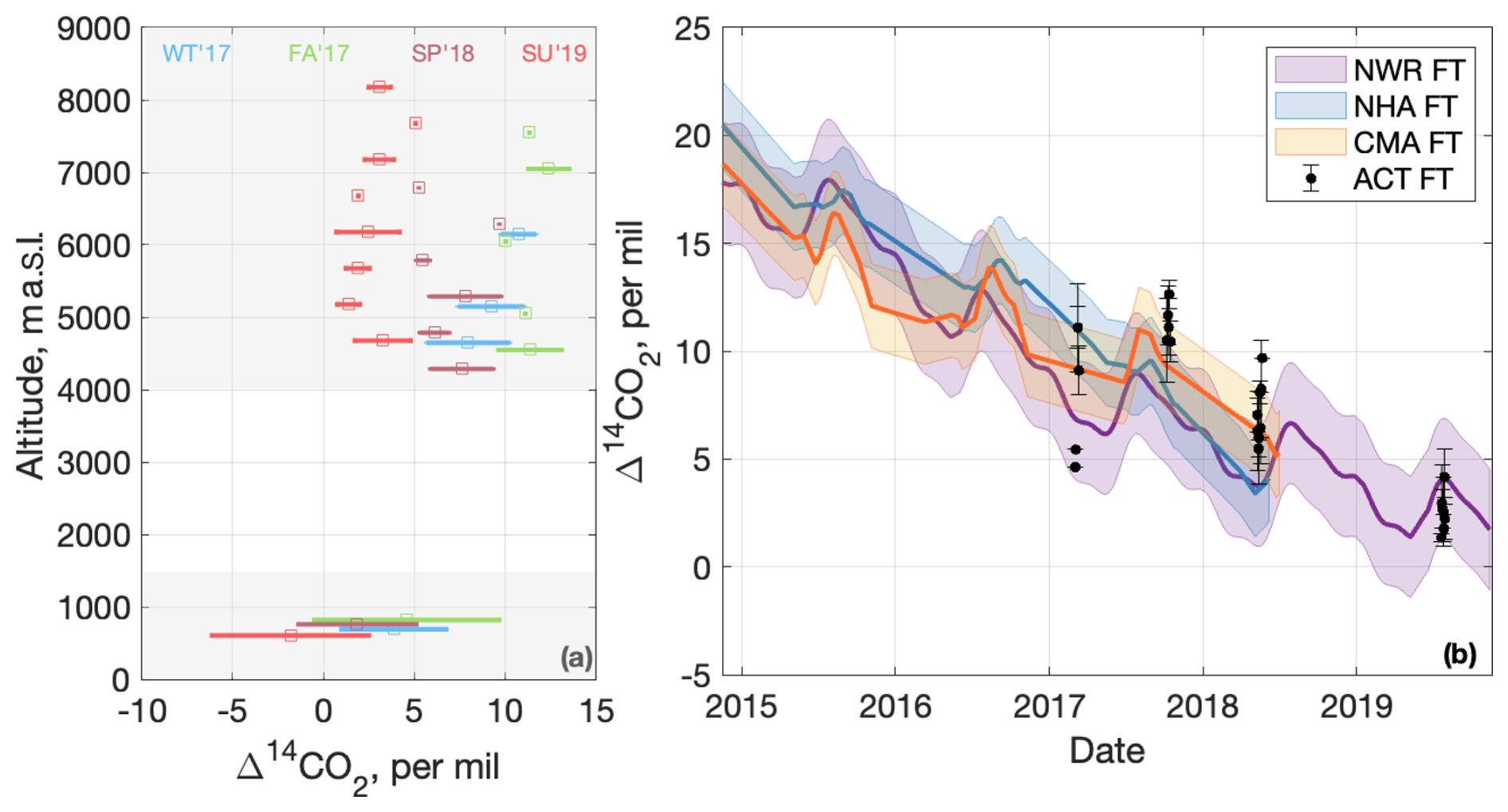
Figure 2 (a) Vertical distribution of Δ¹⁴CO₂ during all ACT campaigns in the Mid-Atlantic USA. ABL values shown are the average of all observations below 1500 m a.m.s.l. (values are separated vertically for clarity) for each seasonal campaign, while horizontal bars represent their 1σ standard deviation in time. FT values (altitudes greater than 4000 m a.m.s.l.) shown are 500 m binned averages and their 1σ standard deviation in Δ¹⁴CO₂ for each 500 m altitude bin. Shaded regions represent ABL and FT definitions. (b) Daily mean ACT FT Δ¹⁴CO₂ background measurements (±1σ standard deviation shading) are shown compared to NOAA GGGRN aircraft network Δ¹⁴CO₂ FT (∼4000 m a.m.s.l.) measurements. GGGRN data are seasonal (3-month averaged) aircraft FT ¹⁴CO₂ obtained offshore of Cape May, NJ (CMA); offshore of Portsmouth, New Hampshire (NHA); and surface Δ¹⁴CO₂ for the high-altitude site Niwot Ridge, CO (NWR), at ∼3500 m a.m.s.l.

Figure 3a highlights the spatial extent of flask sampling during the ACT mission and density of flask sampling over the four seasonal campaigns with an average Δ¹⁴CO₂ ABL minus FT difference of −5 ‰. Using Eq. (4), CO_2ff is calculated for all flask samples, and general agreement between largely negative Δ¹⁴CO₂ ABL signals and higher CO_2ff signals is seen throughout ACT (Fig. 3b). ACT-observed CO_2ff ranges from −0.8 to 15.5 ppm, and we note that negative CO_2ff values are not physically realistic but can occur due to the measurement uncertainty of Δ¹⁴CO₂, by using an inappropriate Δ¹⁴CO₂ background value or by underestimating the CO_2corr term in Eq. (4). Compared to other surface and aircraft observations of CO_2ff throughout the USA, the range of ACT CO_2ff is comparable to CO_2ff measured in other studies in the Mid-Atlantic USA (Miller et al., 2012: −3 to 13 ppm CO_2ff), downwind of Sacramento, CA (Turnbull et al., 2011a: 2.4–8.6 ppm CO_2ff), and in the Colorado urban regions (Graven et al., 2009: 0–20 ppm CO_2ff). Maximum values of CO_2ff measured during ACT were, however, much lower than those over the densely populated urban area of Los Angeles, CA (Miller et al., 2020: −1.3 to 48.4 ppm CO_2ff), due to its more rural sampling focus. Few ACT flight legs were aimed at capturing local urban-scale CO_2ff signals. As such, the analysis below requires averaging of these signals as a more robust way to qualitatively analyze the ACT flask CO_2ff data.

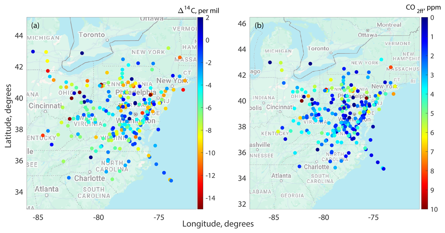
Figure 3 (a) Δ¹⁴CO₂ ABL minus FT differences for all seasons in the Mid-Atlantic USA. Note that the color bar is reversed to indicate warmer colors for more negative Δ¹⁴CO₂. (b) ABL CO_2ff calculated for the same flask samples shown in (a) for all seasons in the Mid-Atlantic USA. Plot maps are produced using Google Maps API (© Google Maps 2025).

3.2 Partitioning of seasonal CO_2tot indicates biogenic-driven variability

For consistency throughout ACT seasonal campaigns, ABL values for all species in the subsequent analysis are reported as an ABL minus FT difference. Figure 4 shows CO_2ff alongside biogenic CO₂ (CO_2bio) calculated from Eq. (1), displayed by month of the year for ACT deployments in winter (2017), spring (2018), summer (2019) and fall (2017) in the Mid-Atlantic United States. Total (CO_2tot), fossil fuel and biogenic CO₂ data are shown to indicate relative contributions to the observed CO_2tot variability (Eq. 1). CO_2tot observed in the ABL varies seasonally; while most often positive for flights conducted in late fall and winter, CO₂ depletion is seen during summer as expected due to net photosynthetic uptake by the terrestrial biosphere (Tans et al., 1990). Seasonal changes in ABL CO_2tot were driven by CO_2bio, which varied from −19.7 ppm during summer flights to 16.2 ppm in late fall (Fig. 4). In early fall, negative CO_2bio was observed (Fig. 4) from a strong surface influence and net uptake in southwestern Virginia (Fig. 1). For the remainder of the fall campaign, flights indicated generally positive CO_2bio with net respiration and weaker surface influence. CO_2ff has a lower contribution to CO_2tot variability during ACT in the Mid-Atlantic region from one campaign to the next, with a positive contribution of 3.3±2.0 ppm. Given the small number of flights shown over 3 years, it should be noted that the seasonality in CO_2ff may not represent true climatological CO_2ff variability and should not be interpreted in terms of uniform fossil fuel emissions, because there is likely seasonal variation in ABL depth, which can counteract seasonally varying emissions.

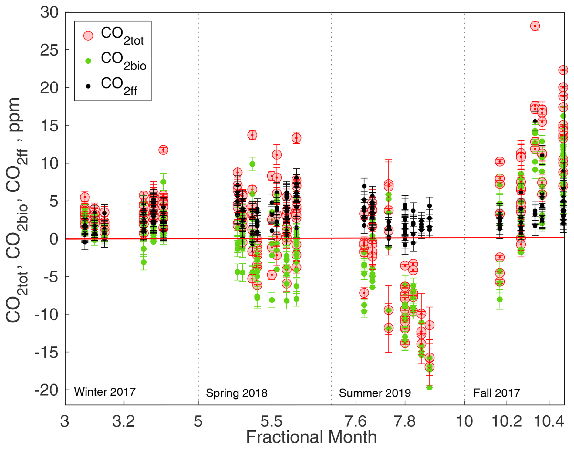
Figure 4 Calculated total CO₂ (CO_2tot), partitioned into biogenic CO₂ (CO_2bio) and fossil fuel CO₂ (CO_2ff) components using Eq. (4) in winter 2017, spring 2018, summer 2019, and fall 2017. As seasonal campaigns were not conducted consecutively within a single year, we examine variability according to a “climatological” year. Note that the x axis is intentionally non-linear to show intra-day variability. 1σ error bars are shown for CO_2tot, CO_2bio and CO_2ff.

The flask sampling region for this study encompasses rural to suburban regions, reducing signal-to-noise ratio in Δ¹⁴CO₂ and complicating the interpretation of CO_2tot observed due to a wide mixture of surface sources (and sinks). As CO_2tot is largely controlled by CO_2bio, we correlate (using Pearson's R² values) and regress CO_2tot with CO_2ff and with CO_2bio (see Table S1 in the Supplement). Regressions between CO_2bio and CO_2tot result in slopes between 0.86 and 0.92 for all seasons. Strong correlations between CO_2bio and CO_2tot exist from spring through to fall with R² values between 0.73 and 0.92. Somewhat strong relationships between CO_2tot and CO_2bio were found during the (March) winter 2017 campaign with a regression slope close to 1 but relatively weak correlation (R²∼0.3), which could partially be explained by small CO_2ff signals but also indicate that observed CO₂ had a non-negligible influence from biogenic CO₂ exchange as was also found in previous studies (Potosnak et al., 1999; Turnbull et al., 2006; Miller et al., 2012; Baier et al., 2020). Correlations between CO_2tot and CO_2ff are weak, with associated regression slopes highest during winter and smaller slopes observed for the spring, summer and fall deployments when ecosystem CO₂ fluxes are higher.

The fraction of negative CO_2tot during biogenically active months in spring (May), summer (July) and fall (October) are 28 %, 62 % and 4 %, respectively (Table S1). However, when examining the fraction of negative CO_2bio (indicating net CO₂ uptake), these percentages are much larger at 57 %, 82 % and 8 %, respectively. The difference between negative CO_2tot and negative CO_2bio fractions of 20 %–30 % during months when the ecosystems are more active highlights the importance of using Δ¹⁴CO₂ to enable partitioning of CO_2tot into fossil fuel and biogenic components; this would not be possible when considering CO_2tot alone, as a portion of this flux component would be masked by fossil fuel emissions.

We also examine carbonyl sulfide ABL minus FT differences (OCS_xs) alongside CO_2bio as an additional tracer for biogenic processing as OCS is taken up by plants similarly to CO₂ but not respired (Montzka et al., 2007; Campbell et al., 2008, Fig. 5). In Fig. 5, we observe a strong positive correlation with CO_2bio and OCS_xs when combining all seasonal ACT data except fall, where CO_2bio is either negative or weakly positive (see Fig. S1a in the Supplement), consistent with photosynthesis explaining negative CO_2bio values. A modest positive correlation (R=0.54) is seen when also including fall ACT data. Including or excluding the winter data, given the insignificant slope between OCS_xs and CO_2bio (Table S1), does not affect this correlation.

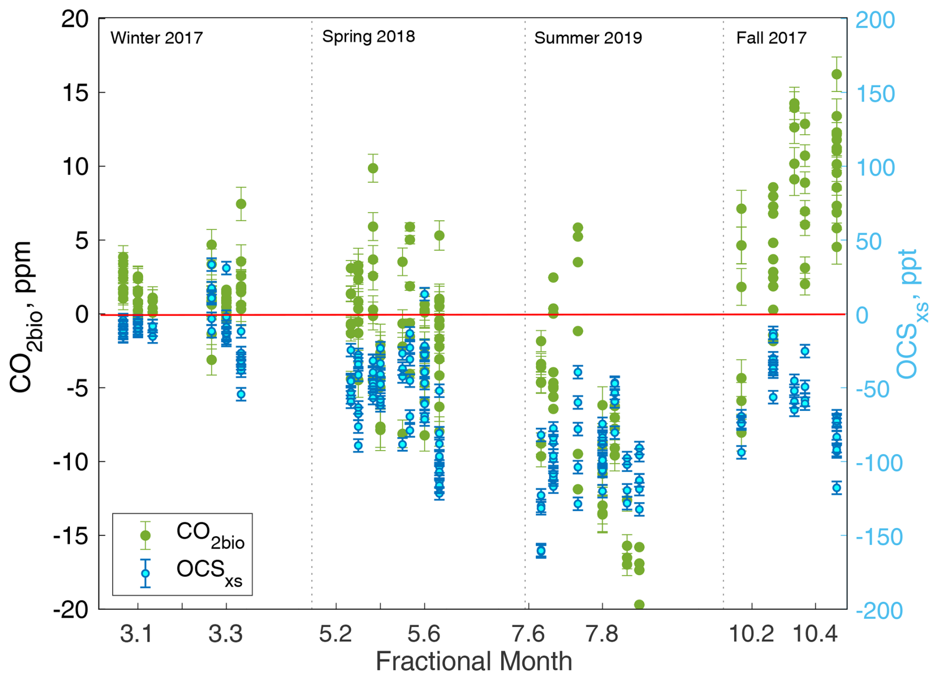
Figure 5 ABL biogenic CO₂ (CO_2bio) and OCS ABL minus FT difference (OCS_xs) in winter 2017; spring 2018; summer 2019; and fall 2017. As seasonal campaigns were not conducted consecutively within a single year, we examine variability according to a “climatological” year. Note that the x axis is intentionally non-linear to show intra-day variability. 1σ error bars are shown for CO_2bio and OCS_xs.

For fall 2017, the overall correlation between CO_2bio and OCS_xs is low and not significant (Table S1). However, statistically significant correlations are seen between negative CO_2bio and OCS_xs in early fall due to continued uptake of CO₂ by the terrestrial biosphere (Fig. 5). A moderate negative correlation is observed between OCS_xs and CO_2bio in late fall after net respiration is seen to occur (Figs. 5 and S1b). During this time, CO_2bio values of up to ∼16 ppm occur alongside relatively significant OCS_xs values of almost −120 ppt. The net negative correlation during fall between CO_2bio and OCS_xs indicates that while CO₂ uptake could still be occurring the magnitude of this process is not large enough to offset respiration. Similar to ACT, clear differences in the amplitude and phases of OCS and CO₂ cycles were first described in Montzka et al. (2007) and in other previous studies (Kuai et al., 2022; Ma et al., 2023). Furthermore, many OCS studies have found several instances where ecosystem OCS uptake is decoupled from gross primary productivity (GPP), including nighttime processes (Commane et al., 2015; Kooijmans et al., 2017; Hu et al., 2021), uptake from soil (Whelan et al., 2022) and/or senescing or decaying fall vegetation (Sun et al., 2016; Rastogi et al., 2018). Further studies could utilize colocated measurements such as OCS and radiocarbon-based CO_2bio to evaluate (a) the relationship between OCS and CO₂ cycles during the transition from net photosynthesis to net respiration and (b) regional model GPP and respiration fluxes. Further, we note that correlations between negative CO_2tot and OCS_xs weaken in the early fall due to proportionally high fossil fuel emissions, providing insufficient information about GPP. Parazoo et al. (2021) found that models underestimate observed CO_2tot during ACT and have decreased fidelity in reproducing GPP inferred from observations throughout the USA. Since stronger relationships emerge between OCS_xs and CO_2bio than OCS_xs and CO_2tot, again, using OCS and radiocarbon-based CO_2bio could further inform and constrain these model processes.

3.3 Example case: “pseudo-CO_2ff” as a product for evaluating model error

We use CO_2ff as a model “transport tracer” to examine model errors as CO_2ff fluxes are assumed to be relatively well-known (Turnbull et al., 2009). Well-known emissions and well-measured mole fractions directly tracing those emissions allow us to evaluate the atmospheric tracer transport that connects the two. Here, we compare a “pseudo-CO_2ff” or high-frequency CO${}_{\mathrm{2}\mathrm{ff}}^{\prime }$ (Eq. 5) to CO_2ffmod simulated using the PSUWRF forward model, based on averaged ODIAC and Miller fossil fuel emissions (Jacobson et al., 2020). This CO${}_{\mathrm{2}\mathrm{ff}}^{\prime }$ product, being high frequency, can also capture more diurnal variability in fossil fuel CO₂ and therefore evaluate modeled fossil fuel CO₂ more thoroughly than measurements made using discrete flask samples.

3.3.1 Variability and uncertainty of R_CO and CO_2ff

Our CO${}_{\mathrm{2}\mathrm{ff}}^{\prime }$ estimation relies on the assumption that the emission ratio of CO to CO_2ff (R_CO) is constant for a given flight day. As mentioned above, a median R_CO value for each day is used as opposed to a more general regression slope between flask CO ABL minus FT differences and CO_2ff because of low correlations between the two variables seasonally. We note that the numerator of R_CO represents the enhancement in all CO sources (fossil, but also potentially biomass burning and oxidation of volatile organic compounds – VOCs) as well as a very small amount of CO oxidative loss. Because all of these sources are “calibrated” relative to CO_2ff (the denominator), it is not necessary to explicitly define non-fossil components of this ratio.

Figure 6 indicates that the median R_CO calculated for all ACT missions (10.03±8.15 ΔCO per ppm CO_2ff; 68 % CI) is slightly higher than in urban studies (Turnbull et al., 2011a, 2015; Miller et al., 2012). Day-to-day or even diurnal R_CO is also largely variable, which could be a result of variability in CO_2ff or in measured background levels (which are represented by a single daily value). Spatial differences in VOC oxidation could play a minor role in influencing the variability of R_CO. CO additions from VOCs throughout the ACT Mid-Atlantic region will render R_CO higher. However, despite the expectation that greater oxidation of VOCs will produce more CO during the summer (Vimont et al., 2017), we see the highest average R_CO values during spring. R_CO variability in both the fall and spring campaigns suggest that there could be other influential mechanisms occurring, yet DiGangi et al. (2021) found that the biomass burning influences on air sampled during ACT were negligible in the Mid-Atlantic region, ruling out the possibility that biomass burning events contribute to the high variability of R_CO calculated here. In general, it is more likely that low CO_2ff signals with high relative uncertainties are creating abnormally high R_CO values using this median method in this work, which has also been found and discussed in great detail in Maier et al. (2024b).

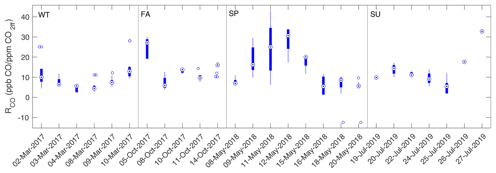
Figure 6 Daily R_CO calculated from discrete flask samples during winter (WT, 2017), fall (FA, 2017), spring (SP, 2018), and summer (SU, 2019). Note that, unlike Figs. 4 and 5, flight data are shown in chronological order. Median R_CO for each research flight is shown as a bullet point, with the interquartile (IQ) range shown as the thick bar line. Outliers greater than 1.5 times the IQ range are shown as separate open circles, and maximum extreme values as whiskers that do not qualify as outliers (thin lines), extending from the IQ ranges. Flask data shown are combined for B-200 and C-130 aircraft.

As mentioned above, we calculate CO${}_{\mathrm{2}\mathrm{ff}}^{\prime }$ only for days when flask measurements were analyzed for Δ¹⁴CO₂. When comparing CO${}_{\mathrm{2}\mathrm{ff}}^{\prime }$ with flask-based CO_2ff, the mean bias is 0.7±2.1 ppm (1σ) (Fig. 7). The relatively large standard deviation in Fig. 7 indicates that flask samples collected within a single research flight were not always representative of the entire domain surveyed on that day by continuous analyzers. Point sources of CO₂ from power plants that do not emit CO captured by continuous measurements could potentially skew this comparison alongside other non-fossil-fuel CO sources, but the small bias between the two suggests that CO${}_{\mathrm{2}\mathrm{ff}}^{\prime }$ is generally in good agreement with flask CO_2ff.

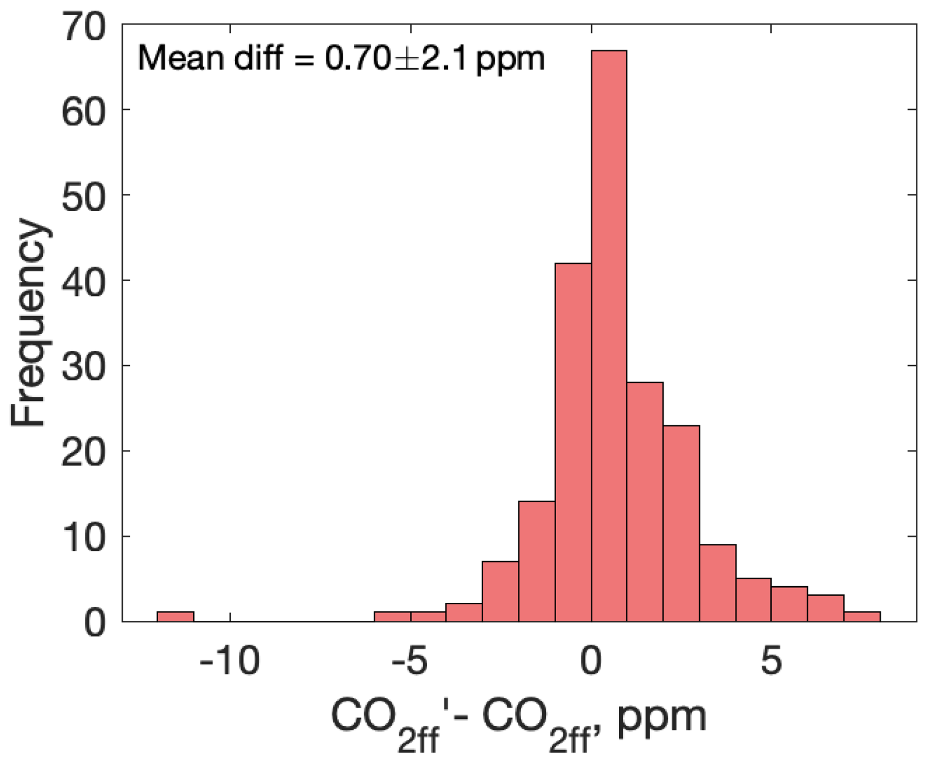
Figure 7 Histogram of in situ (CO${}_{\mathrm{2}\mathrm{ff}}^{\prime }$) minus flask-derived (CO_2ff) fossil fuel CO₂ for measurement times corresponding to the total campaign (winter 2017 through to summer 2019) in the Mid-Atlantic region. Here, CO${}_{\mathrm{2}\mathrm{ff}}^{\prime }$ is calculated for corresponding flask sample times. By definition of CO_2ff and CO${}_{\mathrm{2}\mathrm{ff}}^{\prime }$ above, this comparison indicates ABL sample comparisons only.

3.3.2 Comparison of CO'_2ff and CO_2ffmod

Figure 8 shows the average difference between CO_2ffmod computed along ACT flight tracks and ABL CO${}_{\mathrm{2}\mathrm{ff}}^{\prime }$. Several research flight days indicate rough agreement between CO_2ffmod and CO${}_{\mathrm{2}\mathrm{ff}}^{\prime }$ within a mean of $\sim \mathrm{0.49}\pm \mathrm{2.6}$ ppm (1σ) but higher differences outside of average CO${}_{\mathrm{2}\mathrm{ff}}^{\prime }$ uncertainty bounds are seen in Fig. 8 along with a slight skewness. The mapped extent of this positive bias in CO_2ffmod is visualized in Fig. 9 for fall 2017, spring 2018 and summer 2019 campaigns, while the winter 2017 campaign model bias in CO_2ffmod is slightly negative.

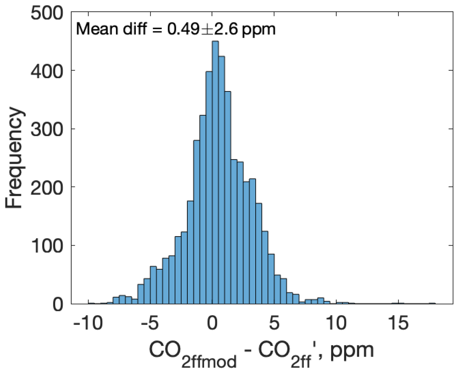
Figure 8 Histogram of PSUWRF CO_2ffmod–CO${}_{\mathrm{2}\mathrm{ff}}^{\prime }$ for all flask Δ¹⁴CO₂ sample days between winter 2017 and summer 2019 in the Mid-Atlantic region.

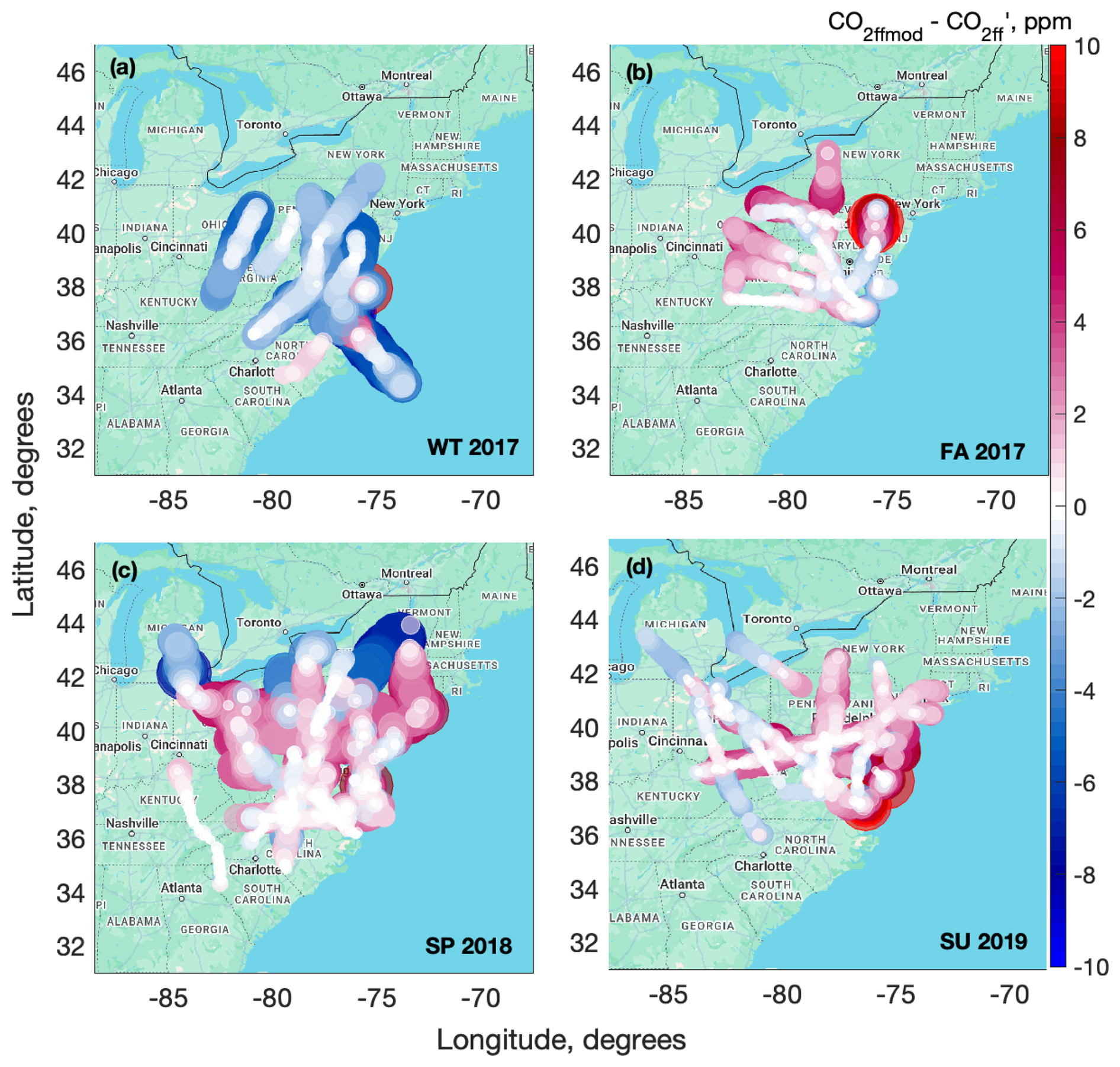
Figure 9 Mapped modeled versus CO${}_{\mathrm{2}\mathrm{ff}}^{\prime }$ for flask Δ¹⁴CO₂ sample flight days for (a) winter (WT) 2017, (b) fall (FA) 2017, (c) spring (SP) 2018 and (d) summer (SU) 2019 campaigns. Points are sized by the model minus data differences. Plot maps are produced using Google Maps API (© Google Maps 2025).

While there are logistical advantages to using this “pseudo-CO_2ff” method from a Δ¹⁴CO₂ measurement capacity standpoint, this product has a higher average uncertainty (4.96 ppm) associated with large intra-day background variability and assumptions in the value of R_CO. For this reason, we caution the overgeneralization of the use of CO_2ff as a transport tracer with this dataset and have chosen 24 July 2019 as an example of when positively biased CO_2ffmod can be evaluated using CO${}_{\mathrm{2}\mathrm{ff}}^{\prime }$. Here, a series of B-200 flights was conducted downwind of three major eastern US cities (New York City, NY; Philadelphia, PA; and Washington, D.C.). ABL flask sampling on each flight leg informed the derivation of CO${}_{\mathrm{2}\mathrm{ff}}^{\prime }$, and both estimates are in rough agreement as seen in Fig. 10. This individual flight day had higher fossil fuel CO₂ signals and lower variability in background CO measurements, with a lower CO${}_{\mathrm{2}\mathrm{ff}}^{\prime }$ uncertainty (∼2 ppm) relative to the campaign-wide average.

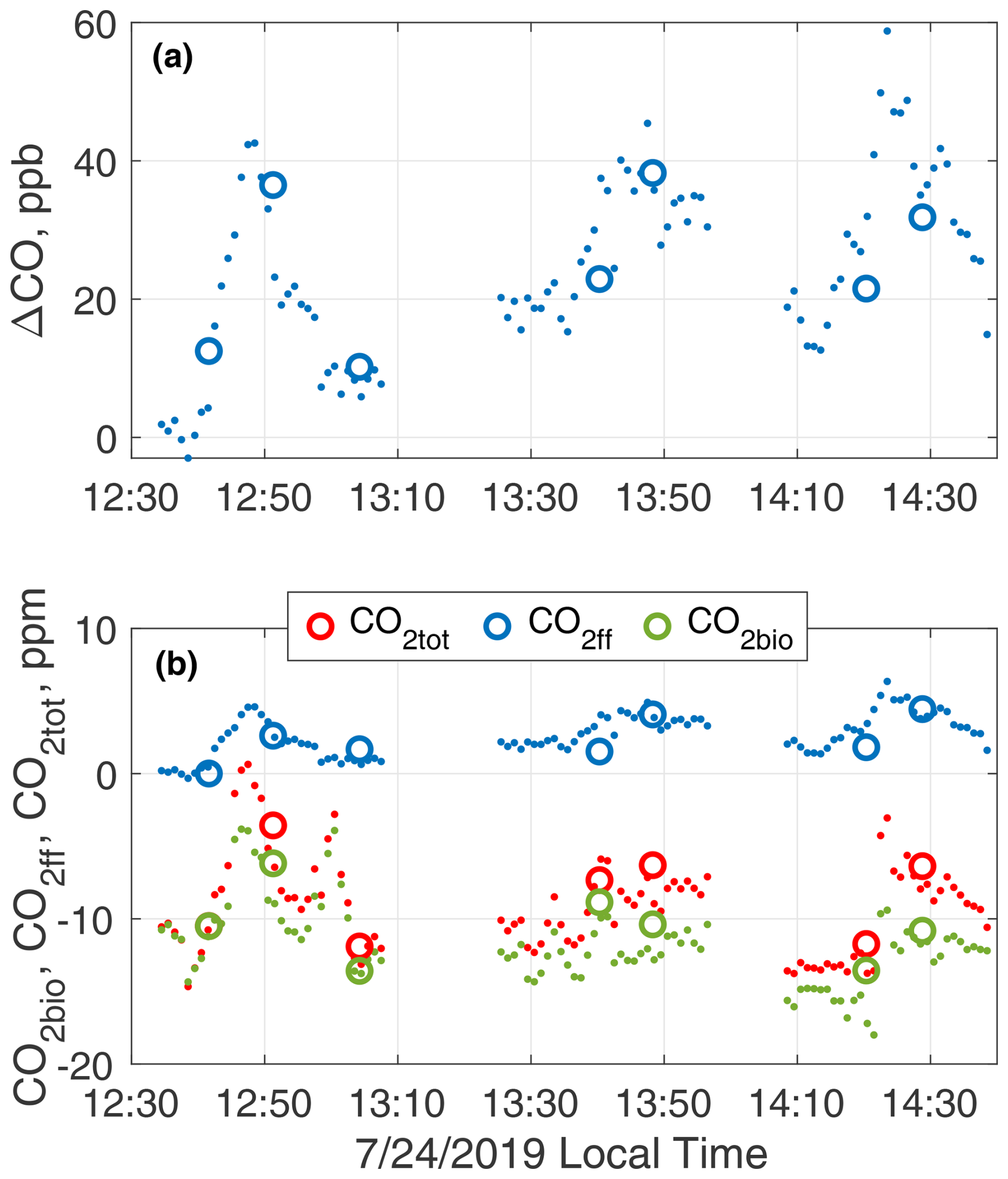
Figure 10 In situ (points) and flask (circles) observations for the B-200 aircraft on 24 July 2019. (a) CO ABL minus FT differences (ΔCO) calculated from flasks and in situ continuous measurements. ΔCO from flasks is used to calculate R_CO and thus CO${}_{\mathrm{2}\mathrm{ff}}^{\prime }$ using Eq. (5) using in situ measurements. The average difference in ΔCO (in situ minus flask) is 0.6±8.7 ppb. (b) CO_2bio, CO${}_{\mathrm{2}\mathrm{ff}}^{\prime }$ and CO_2tot calculated from both in situ high-frequency data (points) and from flask measurements (circles) on 24 July 2019 show good agreement. Average differences in CO_2bio, CO${}_{\mathrm{2}\mathrm{ff}}^{\prime }$ and CO_2tot (in situ minus flask) are $-\mathrm{1.6}\pm \mathrm{1.2}$, 1.2±1.3 and 0.4±1.2 ppm, respectively.

Figure 11 shows calculated CO${}_{\mathrm{2}\mathrm{ff}}^{\prime }$ along three ABL flight legs with large positive fossil fuel CO₂ downwind of these urban areas. Comparing modeled (CO_2ffmod), calculated (CO${}_{\mathrm{2}\mathrm{ff}}^{\prime }$) and flask-derived (CO_2ff) CO_2ff, we find that CO${}_{\mathrm{2}\mathrm{ff}}^{\prime }$ plumes observed downwind of cities do not always align with CO_2ffmod throughout the research flight. Significant differences are observed between CO_2ffmod and CO${}_{\mathrm{2}\mathrm{ff}}^{\prime }$ magnitudes, particularly during the Washington, D.C., flight leg of up to 60 % beyond uncertainty bounds, with the urban emissions plume misaligned (Fig. 11). CO_2ffmod is consistently higher than CO${}_{\mathrm{2}\mathrm{ff}}^{\prime }$ in the Philadelphia flight leg as well, with general agreement in the plume variability. Finally, we note that the PSUWRF model simulates CO_2ff in the New York City flight leg relatively well with respect to flask CO_2ff.

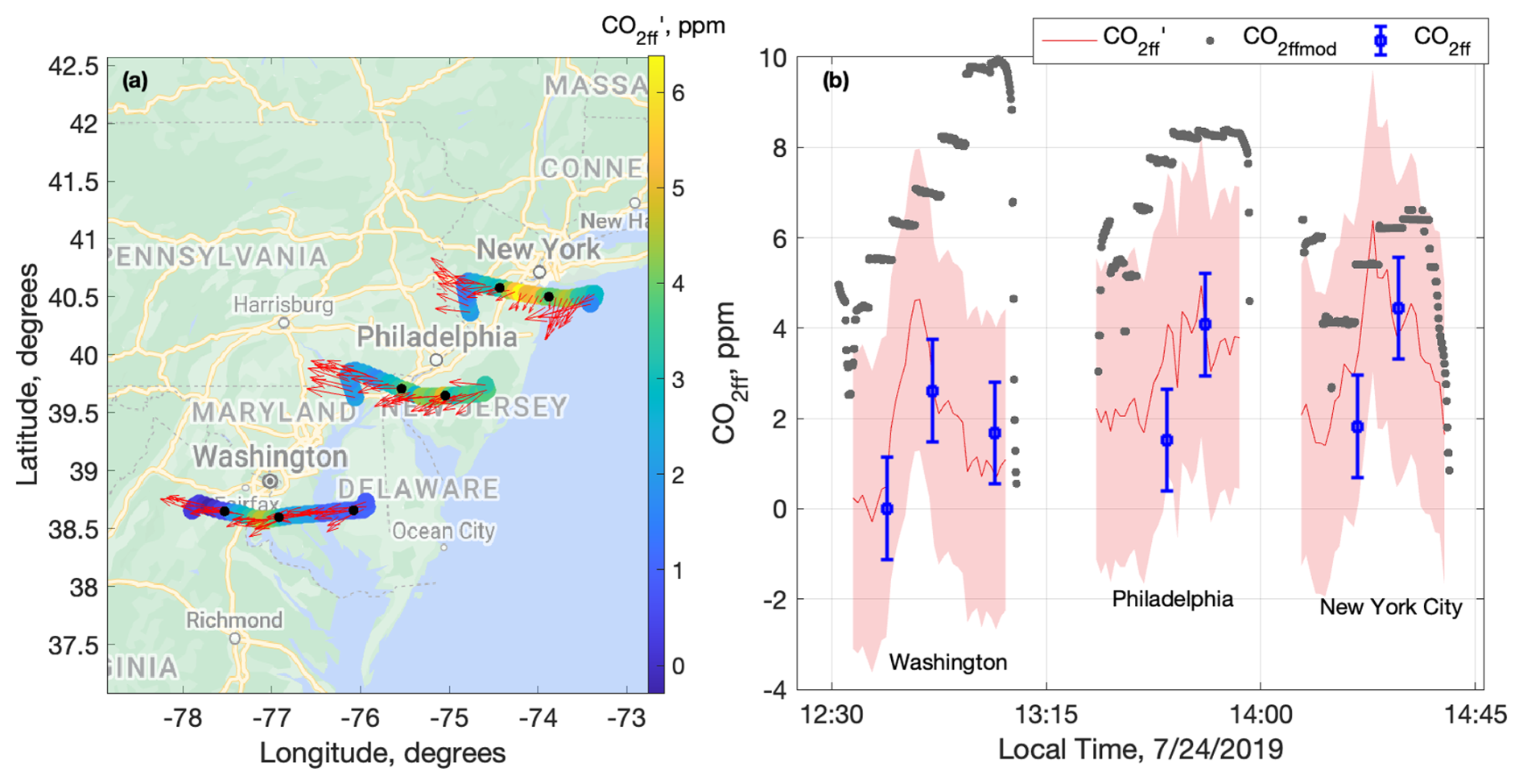
Figure 11 (a) Pseudo-CO_2ff (CO${}_{\mathrm{2}\mathrm{ff}}^{\prime }$) calculated along the ACT B-200 ABL flight track on 24 July 2019 (plot produced using Google Maps API, © Google Maps 2025). Flight tracks are colored by CO${}_{\mathrm{2}\mathrm{ff}}^{\prime }$ which proceed northerly from Washington, D.C., to New York City, NY. Black points indicate flask sample locations. Red arrows indicate the wind direction as calculated from aircraft flight data. (b) Fossil fuel CO₂ calculated from in situ measurements (CO${}_{\mathrm{2}\mathrm{ff}}^{\prime }$), from flask Δ¹⁴CO₂ (CO_2ff) and from PSUWRF using CT fossil fuel emissions (CO_2ffmod). Discretization in CO_2ffmod is due to the native 27 km resolution of PSUWRF. Error shading for CO${}_{\mathrm{2}\mathrm{FF}}^{\prime }$ is the derived 1σ uncertainty in the CO${}_{\mathrm{2}\mathrm{ff}}^{\prime }$ calculation for 24 July 2019 and error bars for flask CO_2ff reflect a 1σ uncertainty.

Current uncertainties of CO₂ fossil fuel fluxes, based on differences among various emissions products, are less than or equal to 20 % at the regional scale (Gurney et al., 2020), and this is corroborated in the PSUWRF model, where Feng et al. (2019a) note that the uncertainty in fossil fuel fluxes on a daily average timescale is approximately 20 %. This uncertainty may increase at the hourly timescale and certainly within smaller urban-scale domains (Gately and Hutyra, 2017). We investigate several reasons for the 60 % overestimation in simulated CO_2ff beyond the larger calculated CO${}_{\mathrm{2}\mathrm{ff}}^{\prime }$ uncertainty bounds and the misalignment of the Washington, D.C., CO_2ffmod “plume” relative to CO${}_{\mathrm{2}\mathrm{ff}}^{\prime }$. First, this discrepancy cannot be explained by model deviations in key meteorological variables such as wind speed, wind direction or ABL depth relative to observations. The PSUWRF modeled wind speeds and directions compare well to in situ wind speed and directions along the B-200 flight track to within 1 m s⁻¹ and 10°, respectively. ABL depths derived from B-200 potential temperature soundings flown at the endpoints of each urban transect in Fig. 11 also compare well with ABL depth, estimated from PSUWRF potential temperature to within 300 m on average. Second, emissions uncertainties within PSUWRF could result in observed differences between CO${}_{\mathrm{2}\mathrm{ff}}^{\prime }$ and CO_2ffmod of this magnitude. One hypothesis is that if multiple fossil fuel emissions datasets are run independently in PSUWRF and the ensemble of these simulations is narrow, then more confidence can be gained in that the differences in Fig. 11 are not due to errors in fluxes but rather errors in model transport. PSUWRF simulations between 2017–2018 indicate that independently run fossil fuel emissions fields with differing spatial and temporal resolutions (i.e., ODIAC and Miller fields) result in small CO_2ffmod differences that are within 1.5–2 ppm on average. While these fossil fuel emissions products were not run separately in the PSUWRF model beyond 2018, a 2 ppm CO_2ffmod variability is substantially smaller than that shown in Fig. 11 downwind of Washington and Philadelphia (3–6 ppm CO_2ff). It is possible that the model vertical transport parameterizations are erroneous earlier in the day, which could produce errors later in the day in CO_2ff accumulation and venting relative to that observed downwind of Washington, D.C., and even Philadelphia, PA. Therefore, while our current results suggest that model transport rather than fluxes are erroneous on this particular flight, the results from this case study are important to document for future model–observation comparisons. More intensive work beyond the scope of this work would be needed to verify our hypothesis, which could involve model runs with a number of both transport and flux variants to discern model variability with different realistic ensemble members. Within this type of study, observed and modeled values for additional urban campaign data should also be compared.

While this example does not represent the average CO_2ffmod bias with respect to CO${}_{\mathrm{2}\mathrm{ff}}^{\prime }$ during ACT, it illustrates the utility of CO_2ff as a model transport tracer. In the above example, the high-frequency CO${}_{\mathrm{2}\mathrm{ff}}^{\prime }$ product is able to easily highlight potential modeled errors in the representation of diurnal CO_2ff plume variability. As discussed in Miller et al. (2020), deriving CO${}_{\mathrm{2}\mathrm{ff}}^{\prime }$ in this way, using information gleaned from a small subset of Δ¹⁴CO₂ flask sample measurements, can provide a means for determining the fossil fuel and biogenic components of CO_2tot for regional or city-scale studies. Despite higher average uncertainties than flask-based methods, comparisons to models might allow for examination and improvements upon gross model errors for more accurate CO₂ mole fraction estimation and process-based studies. As mentioned above, differentiating between regional model transport and flux errors might be improved upon in the future by using an ensemble of both transport and flux variants. As ACT Δ¹⁴CO₂ flask sampling was generally aimed at capturing broad-scale biogenic CO₂ features across the eastern USA, more targeted flask sampling in urban areas with larger CO_2ff signals could reduce R_CO and CO${}_{\mathrm{2}\mathrm{ff}}^{\prime }$ uncertainties, which would allow for more robust Δ¹⁴CO₂-based model verification using comparatively fewer flask samples. At more rural sites, a greater number of flask samples may be needed to robustly calculate CO${}_{\mathrm{2}\mathrm{ff}}^{\prime }$ (Maier et al., 2024b).

4 Conclusions

The ACT-America mission, while focused on improving the accuracy of regional carbon flux estimates, also provided the opportunity for a dense seasonally diverse dataset of atmospheric Δ¹⁴CO₂ measurements from flasks sampled throughout the Mid-Atlantic USA and the capability to disaggregate total CO₂ into biogenic and fossil fuel components, which is critical for regional CO₂ source attribution. Seasonal campaigns occurring between 2017 and 2019 indicated that biogenic CO₂ exchange in the Mid-Atlantic was the primary driver of CO₂ boundary layer variability in this region as expected, while CO_2ff remained relatively constant during the ACT mission. Consistent OCS uptake in all seasons was observed that correlated well with negative CO_2bio, confirming CO₂ uptake by photosynthesis throughout the ACT campaigns, though instances were seen where OCS uptake was clearly decoupled from gross primary productivity during the fall. With the broad nature of flask sampling during ACT, the signal-to-noise (measurement precision) ratio in Δ¹⁴CO₂ data was low, and campaigns investigating strictly urban CO₂ signals can better highlight the utility that routine observations of Δ¹⁴CO₂ can provide, including critical information for stakeholders in assessing carbon reduction strategies on regional to sub-regional scales. Several studies have shown the value of incorporating Δ¹⁴CO₂ alongside CO₂ measurements as an improved model constraint on regional CO₂ fluxes, and future work will require a continued effort to ensure routine Δ¹⁴CO₂ measurements throughout the NOAA GGGRN and other networks. Here, we have used flask Δ¹⁴CO₂ samples, taken alongside continuous in situ CO measurements, to provide a high-frequency “pseudo-CO_2ff” product (CO${}_{\mathrm{2}\mathrm{ff}}^{\prime }$) using the relationship between in situ CO ABL minus FT differences and flask-derived CO_2ff. This product was used to evaluate modeled CO_2ff at a higher temporal resolution than discrete flasks can provide and to illuminate potential errors in model transport at the regional scale. Although the ACT dataset and analysis therein are limited by higher CO${}_{\mathrm{2}\mathrm{ff}}^{\prime }$ uncertainties, as well as limited to days when Δ¹⁴CO₂ signals are higher, this work highlights the value of such a product in future campaigns and measurement networks as a model evaluation tool.