the Creative Commons Attribution 4.0 License.
the Creative Commons Attribution 4.0 License.
 | 09 Sep 2024
Tropical tropospheric ozone distribution and trends from in situ and satellite data
Ilann Bourgeois
Kai-Lan Chang
Jerald Ziemke
Bastien Sauvage
Ryan M. Stauffer
Anne M. Thompson
Debra E. Kollonige
Nadia Smith
Daan Hubert
Arno Keppens
Juan Cuesta
Klaus-Peter Heue
Pepijn Veefkind
Kenneth Aikin
Jeff Peischl
Chelsea R. Thompson
Thomas B. Ryerson
Gregory J. Frost
Brian C. McDonald
Owen R. Cooper
Tropical tropospheric ozone (TTO) is important for the global radiation budget because the longwave radiative effect of tropospheric ozone is higher in the tropics than midlatitudes. In recent decades the TTO burden has increased, partly due to the ongoing shift of ozone precursor emissions from midlatitude regions toward the Equator. In this study, we assess the distribution and trends of TTO using ozone profiles measured by high-quality in situ instruments from the IAGOS (In-Service Aircraft for a Global Observing System) commercial aircraft, the SHADOZ (Southern Hemisphere ADditional OZonesondes) network, and the ATom (Atmospheric Tomographic Mission) aircraft campaign, as well as six satellite records reporting tropical tropospheric column ozone (TTCO): TROPOspheric Monitoring Instrument (TROPOMI), Ozone Monitoring Instrument (OMI), OMI/Microwave Limb Sounder (MLS), Ozone Mapping Profiler Suite (OMPS)/Modern-Era Retrospective analysis for Research and Applications version 2 (MERRA-2), Cross-track Infrared Sounder (CrIS), and Infrared Atmospheric Sounding Interferometer (IASI)/Global Ozone Monitoring Experiment 2 (GOME2). With greater availability of ozone profiles across the tropics we can now demonstrate that tropical India is among the most polluted regions (e.g., western Africa, tropical South Atlantic, Southeast Asia, Malaysia and Indonesia), with present-day 95th percentile ozone values reaching 80 nmol mol−1 in the lower free troposphere, comparable to midlatitude regions such as northeastern China and Korea. In situ observations show that TTO increased between 1994 and 2019, with the largest mid- and upper-tropospheric increases above India, Southeast Asia, and Malaysia and Indonesia (from 3.4 ± 0.8 to 6.8 ± 1.8 nmol mol−1 decade−1), reaching 11 ± 2.4 and 8 ± 0.8 nmol mol−1 decade−1 close to the surface (India and Malaysia–Indonesia, respectively). The longest continuous satellite records only span 2004–2019 but also show increasing ozone across the tropics when their full sampling is considered, with maximum trends over Southeast Asia of 2.31 ± 1.34 nmol mol−1 decade−1 (OMI) and 1.69 ± 0.89 nmol mol−1 decade−1 (OMI/MLS). In general, the sparsely sampled aircraft and ozonesonde records do not detect the 2004–2019 ozone increase, which could be due to the genuine trends on this timescale being masked by the additional uncertainty resulting from sparse sampling. The fact that the sign of the trends detected with satellite records changes above three IAGOS regions, when their sampling frequency is limited to that of the in situ observations, demonstrates the limitations of sparse in situ sampling strategies. This study exposes the need to maintain and develop high-frequency continuous observations (in situ and remote sensing) above the tropical Pacific Ocean, the Indian Ocean, western Africa, and South Asia in order to estimate accurate and precise ozone trends for these regions. In contrast, Southeast Asia and Malaysia–Indonesia are regions with such strong increases in ozone that the current in situ sampling frequency is adequate to detect the trends on a relatively short 15-year timescale.
- Article
(3810 KB) - Full-text XML
-
Supplement
(7050 KB) - BibTeX
- EndNote


Tropospheric ozone negatively affects human health and vegetation, and it is a short-lived climate forcer (Fleming et al., 2018; Mills et al., 2018; Gulev et al., 2021; Szopa et al., 2021). The longwave radiative effect of tropospheric ozone is higher in the tropics and subtropics (between 30° S and 30° N) compared to midlatitudes (Doniki et al., 2015; Gaudel et al., 2018). The most recent Intergovernmental Panel on Climate Change (IPCC) assessment concluded with a high level of confidence that tropical ozone increased by 2–17 % decade−1 in the lower troposphere and by 2–12 % decade−1 in the free troposphere from the mid-1990s to the period 2015–2018 (Gulev et al., 2021). These increases are especially strong across southern Asia (Gaudel et al., 2020), and according to the longest available satellite record, ozone increases in this region have been occurring since at least 1979 (Ziemke et al., 2019). A comprehensive NASA analysis used the Ozone Monitoring Instrument (OMI)/Microwave Limb Sounder (MLS) satellite record to show a clear increase in tropospheric column ozone (1–2.5 DU decade−1) between 2005 and 2016 throughout the tropics, with larger trends over the Arabian Peninsula, India, and Southeast Asia, generally consistent with a simulation by NASA's Modern-Era Retrospective analysis for Research and Applications version 2 (MERRA-2) GMI global atmospheric chemistry model (Ziemke et al., 2019). Similar results were found in a recent study using the NASA Goddard Earth Observing System Chemistry Climate Model (Liu et al., 2022). Weak to moderate positive trends of 0.6 and 1.5 nmol mol−1 decade−1 between 1995 and 2015–2018 were also reported at two remote tropical surface sites (Mauna Loa, Hawaii, and American Samoa, South Pacific; Cooper et al., 2020). A recent analysis of 1998–2019 tropical ozone trends using the Southern Hemisphere ADditional OZonesondes (SHADOZ) network reported highly seasonal but overall weak positive trends (1–2 % decade−1) in the mid-troposphere (5–10 km) (Thompson et al., 2021).
Simulations by a wide range of global atmospheric chemistry models show that global-scale increases in tropospheric ozone since pre-industrial times are driven by anthropogenic emissions of ozone precursor gases (Archibald et al., 2020; Skeie et al., 2020; Griffiths et al., 2021; Szopa et al., 2021; Wang et al., 2022; Fiore et al., 2022), with approximately 54 % of the 1850–2000 global tropospheric ozone increase occurring in the tropics and subtropics (30° S–30° N) (Young et al., 2013). A key ozone precursor that drives the background increase in tropospheric ozone, especially in the free troposphere, is methane (Thompson and Cicerone, 1986a, b; Hogan et al., 1991; Fiore et al., 2002). From 1980 to 2010 the estimated increase in the global tropospheric ozone burden due to the increase in anthropogenic emissions and the partial shift of the emissions from midlatitudes towards the Equator was 28.12 Tg (8.9 %), with the increase in methane (15 %) accounting for one-quarter of the ozone burden increase (as simulated by the CAM-chem model; Zhang et al., 2016). Most of the ozone burden increase (64 %) occurred in the tropics and subtropics (30° S–30° N), driven by emissions from South Asia and Southeast Asia as well as by increasing background methane levels (Zhang et al., 2021). Similar rates of ozone burden increases, peaking in the tropics, are simulated by a range of CMIP6 models (1995–2014) (Skeie et al., 2020), the GEOS-Chem model (1995–2017) (Wang et al., 2022), the JPL TCR-2 chemical reanalysis (1995–2018) (Miyazaki et al., 2020), and a 15-member initial-condition ensemble generated from the CESM2-WACCM6 chemistry–climate model (1950–2014) (Fiore et al., 2022). The increase in methane has continued to the present and the observed global mean methane increase from 1983 to 2023 is 18 % (the increase is 8 % since 2004 when OMI began operations) (https://www.gml.noaa.gov, last access: 20 August 2024). Under a future scenario of high anthropogenic emissions and continuously increasing methane concentrations (Griffiths et al., 2021), the global ozone burden is expected to increase for the remainder of the 21st century (see the ssp370 scenario in Fig. 6.4 of Szopa et al., 2021), with increases of approximately 10 % from 2014 to 2050. In the tropics the strongest increases (though 2050) are expected across South Asia (10 %–20 %), with little or no increase across the remote regions of the equatorial Pacific and equatorial Atlantic.
The tropics are characterized by high ozone values over the southern tropical Atlantic and Southeast Asia (Fishman et al., 1990, 1996; Thompson et al., 1996; Logan, 1999; Ziemke et al., 2019) and low ozone values (< 10 nmol mol−1) in the free troposphere over the Pacific warm pool (Kley et al., 1996), although these low values have become less frequent over the last 2 decades (Gaudel et al., 2020). The spatial distribution of tropical tropospheric ozone (TTO) can vary on a range of timescales. On multiyear timescales TTO experiences a dipole oscillation across the tropical Pacific Ocean due to the El Niño–Southern Oscillation (ENSO) (Chandra et al., 1998; Doherty et al., 2006; Oman et al., 2013; Xue et al., 2020). On seasonal timescales ozone can vary with the Madden–Julian oscillation (MJO) (Ziemke et al., 2015) and also with dry and wet conditions (also called the biomass burning and monsoon seasons) related to the seasonal shifts of the Intertropical Convergence Zone (ITCZ) (Fishman et al., 1992; Oltmans et al., 2001; Sauvage et al., 2007a, b; Thompson et al., 2012; Tsivlidou et al., 2023). In a given season, TTO can be further influenced by biomass burning, lightning, inter-hemispheric transport, and stratospheric intrusions and/or large-scale subsidence (Sauvage et al., 2007a, b; Jenkins et al., 2014; Yamasoe et al., 2015; Hubert et al., 2021; Tsivlidou et al., 2023). For instance, high ozone concentrations were recently measured above the tropical Atlantic (Bourgeois et al., 2020) and were attributed to biomass burning emissions, whose effects on tropospheric ozone enhancements are underestimated by global chemistry transport models, especially in the tropics and the Southern Hemisphere (Bourgeois et al., 2021).
While decades of research on the distribution of TTO using satellite instruments (Fishman et al., 1986, 1990; Fishman and Larsen, 1987; Ziemke et al., 1998, 2005, 2009, 2011, 2019) and in situ observations (Logan, 1999; Thompson et al., 2000, 2003, 2012, 2021; Oltmans et al., 2001; Sauvage et al., 2005, 2007a, b; Yamasoe et al., 2015; Tarasick et al., 2019; Cooper et al., 2020; Lannuque et al., 2021; Tsivlidou et al., 2023) has characterized the spatial and temporal variability of TTO concentrations, reconciling differences between satellite and in situ observations has been a challenge (Gaudel et al., 2018).
To update our understanding of tropospheric ozone's distribution and trends across the tropics, this study presents a quantitative analysis of four complementary datasets in time and space across the 20° S–20° N latitude band: (1) thousands of vertical ozone profiles from the In-Service Aircraft for a Global Observing System (IAGOS) (Nédélec et al., 2015; Blot et al., 2021) above five continental regions, (2) regular vertical profiles from the SHADOZ network (Thompson et al., 2017; Stauffer et al., 2022) above 14 continental and oceanic sites, (3) vertical profiles from the Atmospheric Tomographic Mission (ATom) aircraft campaign above five oceanic regions and (4) tropospheric column ozone retrievals from four well-known and two new satellite records.
The paper is organized as follows. Section 2 describes the datasets and the methodology for quantifying the distribution and trends of ozone. Section 3 presents the results that include the distribution of ozone from the in situ data, an evaluation of the satellite records, and the trend estimates from IAGOS, SHADOZ, and satellite records. Section 4 presents the main conclusions.
We define the tropics as the latitude band between 20° S and 20° N, within the bounds of the Tropic of Cancer and the Tropic of Capricorn. This latitude band covers most of the Southern Hemisphere ADditional OZonesondes (SHADOZ) network designed to measure ozone in the subtropics and tropics. The goal of the study is to characterize the 20° S–20° N latitude band that can be impacted by subtropical air masses in some regions, especially at the edge of the domain.
The satellite data are shown for the same latitude domain.
We focus on three time periods: 2014–2019, also called the “present day”, to assess the distribution of TTO (5th, 50th, and 95th percentiles) with in situ data above the sampled regions and sites described in Fig. 1; 1994–2019 to assess ozone trends using in situ data records for more than 2 decades; and 2004–2019 to assess ozone trends over the time period of the Ozone Monitoring Instrument (OMI) dataset, which is the longest time series of ozone measured from space from a satellite.
We also use new datasets to assess the distribution of TTO, such as the ATom aircraft campaign, as well as the Cross-track Infrared Sounder (CrIS) and Infrared Atmospheric Sounding Interferometer (IASI)/Global Ozone Monitoring Experiment 2 (GOME2) satellite records.
2.1 In situ measurements
2.1.1 IAGOS
The European research infrastructure In-service Aircraft for a Global Observing System (IAGOS), formerly known as the Measurement of Ozone and Water Vapor by Airbus In Service Aircraft (MOZAIC), has collected continuous high-quality ozone profiles up to 12 km (∼ 200 hPa) on board commercial aircraft since 1994 (Blot et al., 2021). Ozone is measured using an ultraviolet (UV) analyzer (Thermo Scientific, model 49) and the total uncertainty is ±2 nmol mol−1 ± 2 % (Nédélec et al., 2015).
For this study, we consider five tropical regions: the Americas, Africa, India, Southeast Asia, and Malaysia and Indonesia. We use IAGOS data to assess the average ozone distribution between 2014 and 2019, referred to as “present-day ozone”, as well as to assess ozone trends between 1994 and 2019. Over the time period 1994–2019, the most frequented airports were Caracas (1214 profiles) and Bogotá (560 profiles) for the Americas; Lagos (761 profiles) and other airports in the Gulf of Guinea for western Africa; Chennai (680 profiles) and Hyderabad (552 profiles) for India; Bangkok (1535 profiles) and Ho Chi Minh City (367 profiles) for Southeast Asia; and Singapore (265 profiles), Kuala Lumpur (208 profiles), and Jakarta (113 profiles) for Malaysia and Indonesia (Table S1 in the Supplement). All available ozone profiles from these airports are used in this study. The individual ozone profiles are averaged to a common vertical resolution of 10 hPa prior to any further analysis. To assess the annual ozone distribution the profiles are averaged annually. To assess ozone trends, the quantile regression method is applied to individual profiles (Sect. 2.5). To compare with the satellite data, the profiles were averaged monthly before being converted to a tropospheric column value ranging from the surface up to 270 hPa or up to the maximum altitude (∼ 200 hPa). We chose 270 hPa to be consistent with the TROPOspheric Monitoring Instrument (TROPOMI) tropical tropospheric column ozone. While some of the satellite records used in this study have an upper limit at 150 hPa (thermal tropopause), IAGOS commercial aircraft do not reach these altitudes.
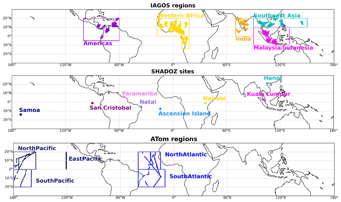
Figure 1Regions and sites of IAGOS, SHADOZ, and ATom measurements used in this study to assess the 5th, 50th, and 95th percentiles of ozone in the tropical troposphere over 2014–2019. Data from IAGOS and ATom flights are clustered into specific regions such as the Americas, western Africa, India, Southeast Asia, Malaysia and Indonesia, North Pacific, South Pacific, eastern Pacific, North Atlantic, and South Atlantic. IAGOS and ATom flight tracks are plotted on the map to show the specific sampling locations for 2014–2019. IAGOS and SHADOZ data are statistically fused above the Americas, Southeast Asia, and Malaysia and Indonesia and used to estimate ozone trends between 1994 and 2019. For India, only IAGOS data are available for the ozone trend estimate between 1994 and 2019.
2.1.2 SHADOZ
The Southern Hemisphere ADditional OZonesondes (SHADOZ) network has provided ozone profiles at multiple sites between 25° S and 21° N since 1998 and presently operates 14 sites. SHADOZ is a NASA-sponsored project operated by NOAA and 15 institutions around the world (Thompson et al., 2003a, b, 2012, 2021). The SHADOZ ozone profiles, measured by electrochemical concentration cell (ECC) ozonesondes, were reprocessed in 2016–2018 (Witte et al., 2017, 2018). In comparisons of the reprocessed data with collocated total ozone spectrometers and satellite overpasses, the reprocessed SHADOZ total ozone column (TOC) disagreed with the independent data within 2 % (Thompson et al., 2017). SHADOZ data since 2018 have been collected and processed according to the same protocols as the reprocessed profiles (Stauffer et al., 2018, 2020, 2022; WMO/GAW 268 Report, 2021). A recent study of TOC stability over 60 global stations revealed an artifact of declining tropospheric ozone at the SHADOZ Hilo and Costa Rican stations (Stauffer et al., 2020, 2022). Those data were not used in the recent Thompson et al. (2021) study that showed distinctive seasonal and regional variations in ozone trends collected at eight SHADOZ stations within ±15° latitude of the Equator.
As with the IAGOS data, the SHADOZ ozone profiles were averaged to a common vertical resolution of 10 hPa before any further analysis. The 10 hPa resolution vertical profiles are fused with the IAGOS 10 hPa-resolution vertical profiles to assess trends between the surface and 200 hPa (Sect. 2.6). To compare with the satellite data, the profiles were averaged monthly before being converted to tropospheric columns up to 270, 150 and 100 hPa.
2.1.3 ATom
The Atmospheric Tomography (ATom) project was a global-scale NASA aircraft mission which collected profiles of ozone and hundreds of other atmospheric constituents in remote regions above the Atlantic and Pacific basins on board the NASA DC-8 aircraft. The project consisted of four seasonal circumnavigations of the globe, one in each season, continually profiling the troposphere between 180 m and 14 km above sea level (a.s.l.) with a temporal resolution of 10 Hz, averaged to 1 Hz (data available at https://espo.nasa.gov/atom, last access: 7 March 2022). The ATom mission occurred in July–August 2016 (ATom-1), January–February 2017 (ATom-2), September–October 2017 (ATom-3), and April–May 2018 (ATom-4). Ozone was measured using the National Oceanic and Atmospheric Administration (NOAA) nitrogen oxide and ozone (NOyO3) instrument (Bourgeois et al., 2020). The total estimated uncertainty at sea level is ± (0.015 nmol mol−1 ± 2 %).
We used the ATom ozone profiles available above five regions in the tropics: North Pacific, South Pacific, eastern Pacific, North Atlantic, and South Atlantic. Most of the regions were sampled over 1 day in August 2016, February and October 2017, and May 2018, except the eastern Pacific which was sampled in July 2016, January and September 2017, and April 2018. Each flight produced 6–14 profiles in each region. Therefore, the ATom dataset is used to assess the ozone distribution over the 2016–2018 time period and for the annual comparison with the satellite products. As for IAGOS and SHADOZ, we averaged the profiles to a common vertical resolution of 10 hPa within the five ATom regions. To compare with satellite data, the profiles were converted to tropospheric column ozone from the near-surface measurements up to 270 hPa and averaged for the entire ATom period above each of the five regions.
2.2 Tropical Tropospheric Column Ozone (TTCO) estimation from IAGOS, SHADOZ, and ATom
In this study and as mentioned in Sect. 2.1, the ozone profiles from in situ observations have been converted to columns to evaluate the satellite products. The current TOAR-II Harmonization and Evaluation of Ground-based Instrument for Free Tropospheric Ozone Measurements (HEGIFTOM) focus working group (https://hegiftom.meteo.be/, last access: 20 August 2024) recommended 150 hPa as the top limit of the TTCO in the 15° S–15° N tropical band and 200 hPa in the 15–30° S and 15–30° N bands. As we focus our study on the 20° S–20° N latitude band, we decided to use the 150 hPa top limit. Some variations on the TTCO definition occur in this study and are detailed below but are not corrected for.
IAGOS aircraft cannot reach 150 hPa as they have a maximum cruise altitude of around 200 hPa. Therefore, only SHADOZ ozonesondes, which reach the middle or upper stratosphere, were used to calculate TTCO from the surface to 150 hPa. However, we additionally calculated TTCO up to 270 hPa with IAGOS and ATom to compare with TROPOspheric Monitoring Instrument (TROPOMI) and Infrared Atmospheric Sounding Interferometer (IASI)/Global Ozone Monitoring Experiment 2 (GOME2) satellite data.
2.3 Satellite data
In this study we mainly focus on satellite data based on ultraviolet (UV) absorption retrievals, supplemented with two ozone records derived from infrared (IR) measurements as described below. Two key parameters differ between the satellite datasets: (i) the top limit used to define the tropospheric column ozone and (ii) the horizontal coverage. Figure S1 in the Supplement shows the time series of the pressure level characterizing the top limit. Depending on the datasets, the top limit is constant or varies with time. The tropical coverage is 20° S–20° N for all satellite records. All satellite records were averaged to a common 5° × 5° monthly grid.
2.3.1 TROPOMI CCD
The TROPOspheric Monitoring Instrument (TROPOMI; Veefkind et al., 2012) was launched on board the Sentinel-5 Precursor (S5P) satellite in October 2017. The tropospheric column ozone data from TROPOMI, inferred using the convective cloud differential technique (CCD; Ziemke et al., 1998; Heue et al., 2016; Hubert et al., 2021), cover the 20° S–20° N latitude band between the surface and 270 hPa. For this study, we compute monthly data from daily measurements on a 5° × 5° grid to be consistent with the other satellite data records. For the 5° × 5° gridded data we estimate the uncertainty of the TROPOMI CCD tropospheric ozone column to be about 2 DU. We only use data from 2019, which is the last year of our present-day time period of 2014–2019.
2.3.2 OMI CCD
The Ozone Monitoring Instrument (OMI) was launched on board the Aura satellite in July 2004. For this study we used tropical tropospheric column ozone retrieved using the CCD technique (Ziemke et al., 1998; Ziemke and Chandra, 2012), which is consistent with TROPOMI-derived TTCO. The tropospheric column is defined between the surface and 100 hPa, and it covers the 20° S–20° N latitude band inherent to the CCD technique. OMI records are available since 2004, and for this study we use monthly means to assess ozone distribution during the present-day time period of 2014–2019 as well as the trends of ozone over 2004–2019. The monthly accuracy and precision (1σ) are 3 and 3.5 DU, respectively.
2.3.3 OMI/MLS
The OMI and the Microwave Limb Sounder (MLS) sensors are both on board the Aura satellite and the tropospheric column ozone is retrieved by subtracting the stratospheric column ozone measured by MLS from the total column ozone measured by OMI (Ziemke et al., 2006). The top limit of the OMI/MLS tropospheric column ozone is the thermal tropopause calculated from NCEP reanalysis data using the World Meteorological Organization (WMO) 2 K km−1 lapse-rate definition. The tropopause varies seasonally between 95 and 115 hPa (Fig. S1). OMI/MLS data cover the 60° S–60° N latitude band, and for this study we focus on the 20° S–20° N latitude band. The monthly accuracy and precision (1σ) are 2 and 1.5 DU, respectively. Further details on the OMI/MLS product and a description of an updated drift correction can be found in Sect. S4 in the Supplement.
2.3.4 OMPS/MERRA-2
The Ozone Mapping Profiler Suite (OMPS) was launched in January 2012 on board the Suomi National Polar-orbiting Partnership (Suomi NPP) spacecraft. The tropospheric column ozone is retrieved by subtracting the stratospheric column of MERRA-2 (Modern-Era Retrospective analysis for Research and Applications version 2) ozone reanalysis data from the total column ozone of the OMPS nadir mapper (Ziemke et al., 2019). The derived daily tropospheric column ozone uses the MERRA-2 tropopause with assimilated MLS ozone. The MERRA-2 tropopause was determined using a potential vorticity (PV) – potential temperature (θ) definition (2.5 PV units, 380 K; Wargan et al., 2020). The tropopause at a given grid point was taken as the larger of these two PV and θ surfaces. However, in this study, the tropopause is exclusively defined by θ surfaces as we focus on the 20° S–20° N latitude band. For the MERRA-2 assimilation, in 2015 MLS changed from version 2.2 to version 4.2 (Wargan et al., 2017; Davis et al., 2017). This produced a 1–1.5 DU difference between the earlier and later record for stratospheric column ozone, which prevents accurate trend detection from either MERRA-2 stratospheric column ozone or the derived tropospheric column ozone from OMPS/MERRA-2. The OMPS/MERRA-2 tropopause pressure varies seasonally between 95 and 108 hPa (Fig. S1). The monthly accuracy and precision (1σ) are 3 and 2 DU, respectively.
2.3.5 CrIS
The Cross-track Infrared Sounder (CrIS) is on board the Suomi NPP (2011–2021) and JPSS-1 (NOAA-20 in operations; 2017–present) and builds upon the hyperspectral IR record first started by the Atmospheric Infrared Sounder (AIRS) on Aqua (2002–2022). For this study we focus on the ozone profiles retrieved by the Community Long-term Infrared Microwave Combined Atmospheric Product System (CLIMCAPS; Smith and Barnet, 2019, 2020). CLIMCAPS retrieves atmospheric state parameters, including ozone profiles (from the surface to the top of the atmosphere), from AIRS and CrIS to form a long-term record that spans instrument and platform differences. CLIMCAPS uses MERRA-2 as the a priori for ozone. Here we focus on CLIMCAPS from CrIS on board Suomi NPP (National Polar-orbiting Partnership, 1 January 2016 to 31 March 2018) and NOAA-20 (previously known as JPSS-1, 1 April 2018 to 31 August 2022) for the time period 2016–2019 because this gives us the baseline IR sounding capability for the next 2 decades (CrIS is scheduled for launch on three additional JPSS platforms). CrIS data cover the 90° S–90° N latitude band, and for this study we focus on the 20° S–20° N latitude band. The accuracy of CrIS tropospheric ozone data varies between −9.4 % globally and −20 % in the tropics compared with ozonesondes. The precision is 21.2 % globally (Nalli et al., 2017).
For CrIS, we accessed CLIMCAPS Level 2 retrievals via NASA GES DISC (NASA Goddard Earth Sciences Data and Information Services Center; Sounder SIPS and Barnet, 2020a, b; https://disc.gsfc.nasa.gov/, last access: 22 August 2024). We aggregated them onto 1° equal-angle global grids. Specifically, we accessed the ozone retrieved fields (o3_mol_lay) defined as 100-layer column density profiles [molec. m−2] and subset them into tropospheric profiles. We defined the troposphere as all values between the Earth's surface (prior_surf_pres) and the tropopause (tpause_pres). A total column value is simply the sum of all column density values converted to DU. We used the quality flag (ispare_2 = 0) to define all successful retrievals, which we simply averaged per grid box. No other filtering was done. CLIMCAPS retrievals are done from cloud-cleared radiances, so we do not have to make specific accommodation for clouds.
2.3.6 IASI/GOME2
IASI/GOME2 is a multispectral approach used to retrieve ozone for several partial columns. It is based on the synergism of IASI and GOME-2 measurements in the thermal infrared and the ultraviolet spectral domain, respectively, jointly used in terms of radiance spectra for enhancing the sensitivity of the retrieval for lowermost-tropospheric ozone (below 3 km above sea level; see Cuesta et al., 2013). Studies over Europe and East Asia have shown good skill for capturing near-surface ozone variability compared to surface in situ measurements of ozone (Cuesta et al., 2018, 2022). This ozone product offers global coverage for low-cloud-fraction conditions (below 30 %) for 12 km diameter pixels spaced by 25 km (at nadir pointing). The IASI/GOME2 global dataset is publicly available through the AERIS French data center, with data from 2017 to the present (available at https://iasi.aeris-data.fr/o3_iago2/, last access: 22 August 2024), and covers the 90° S–90° N latitude band. For this study, we use the 2017–2021 monthly tropospheric column ozone between the surface and 12 km, focusing on the 20° S–20° N latitude band.
2.4 Comparison between satellite and in situ data
To assess the performance of the six satellite records, we calculated the mean biases between satellite-detected monthly TTCO and IAGOS as well as SHADOZ integrated profiles over the 2014–2019 time period. The biases are calculated as follows.
N is the number of monthly TTCO observations over a given region or site and yi is the monthly mean TTCO based on in situ data (ref) or satellite data (sat).
In order to represent the relationship between the satellite data and the in situ data, we used a least-square linear regression as well as the orthogonal distance regression (ODR). In this exercise, we do not use strict sampling criteria in time and space (except for the satellite and in situ observations being in the same month, year, and grid cell) or smoothing of in situ ozone profiles to the vertical resolution of the satellite data before integration. To extract satellite data over IAGOS and ATom regions, we used a 5° × 5° gridded mask reflecting monthly grid cells with available IAGOS and ATom data, and only these grids are used to compute regional mean satellite values. For comparison to SHADOZ data, satellite data were extracted at the latitude and longitude of the SHADOZ sites (sonde launch site within satellite pixel). We include all satellite records with a minimum of 1 year of data within 2014–2019.
2.5 Fused product and trend estimation
The tropical region has sparse in situ sampling in both time and space, which makes accurate quantification of trends challenging. Based on a sampling sensitivity test (Sects. S1, S2, Figs. S2 and S3), we conclude that one profile per week is only sufficient for detection of trends with a very strong magnitude (i.e., nmol mol−1 decade−1), which is not common in the free troposphere. We show that a sampling frequency of seven profiles per month is sufficient for basic trend detection (i.e., to reliably determine if there is a trend) of TTO using the datasets presently available (if the magnitude of a trend is greater than nmol mol−1 decade−1), but additional data are required for accurate quantification or detection of a weaker trend.
Because the sparse sampling makes trend detection difficult, we have chosen to statistically fuse the in situ measurements from the IAGOS and SHADOZ programs over large regions, which includes air masses from different origins and influences (Figs. 1 and S12 to S16). The method is based on a data fusion technique described by Chang et al. (2022), which considers ozone correlation structure, sampling frequency, and inherent data uncertainty. By investigating systematic ozone variability, the resulting fused product allows us to reconcile the differences between heterogeneous datasets and enhance the detectability of trends. For the Americas, we fused SHADOZ data over San Cristóbal and Paramaribo with the IAGOS data (Fig. S12). For Southeast Asia, we fused SHADOZ over Hanoi with the IAGOS data (Fig. S13). For Malaysia and Indonesia, we fused SHADOZ data over Kuala Lumpur and Watukosek (Java) with the IAGOS data (Fig. S14). For western Africa and India, SHADOZ data are not available and we show the time series of just the IAGOS data in Figs. S15 and S16, respectively.
For IAGOS data and the fused product, the trend estimate and its associated uncertainty are based on quantile regression (Koenker and Hallock, 2001), which is an appropriate choice for ozone profile time series because of the irregular sampling schemes and the need to evaluate ozone changes associated with a range of percentiles (Chang et al., 2021). Data gaps are not interpolated as interpolation creates fictitious sample sizes for trend detection, while treating the missing data as not substantially deviant from the available data variability. Due to limited available sample sizes, only median trends (i.e., an estimate of the trend based on the median change in data distribution) are reported in this study. It should be noted that quantile regression is specifically designed to evaluate the distributional changes (determined by all available profiles). Although trends in extreme percentiles are not considered due to insufficient samples, by focusing on the median changes, our trend estimates are expected to be more robust against extreme variability or less impacted by potential large sampling bias (due to imbalanced sampling). The R and Python codes for implementing quantile and median regression are provided in the TOAR statistical guidance note (Chang et al., 2023). To account for potential correlation between ozone and climate variability, such as ENSO (El Niño–Southern Oscillation) and QBO (quasi-biennial oscillation), the trend model is specified through
where b0 is the intercept, b1 is the linear trend, b2 is the regression coefficient for ENSO, and b3 and b4 are coefficients for QBO at 30 and 50 mb, respectively. The trend uncertainty is derived by a bootstrapping method (Feng et al., 2011). The ENSO and QBO indexes can be found in the “Data availability” section. Figure S17 shows that if ENSO and QBO are not considered, the trends can be offset by about 1–2 nmol mol−1 decade−1 at individual pressure layers over the five IAGOS regions, except Africa where the trend differences are negligible.
In addition, we conducted trend analysis of the monthly TTCO from SHADOZ, IAGOS, OMI, and OMI/MLS as well as the tropical ozone burden (TOB, Tg decade−1) over zonal monthly means using OMI and OMI/MLS. The OMI/MLS TTCO has shown a drift over time that we corrected for this study (see Sect. S4).
3.1 Ozone profiles
For the period 2014–2019 (IAGOS, SHADOZ) and 2016–2018 (ATom), the three in situ datasets show a range of ozone values from the surface to 200 hPa, indicative of the different photochemical and transport regimes across the tropics (Fig. 2). Here we highlight several notable features.
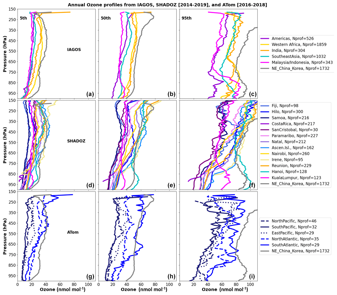
Figure 2Distribution of tropical tropospheric ozone (TTO) showing annual 50th (a, d, g), 5th (b, e, h), and 95th (c, f, i) percentiles of ozone profiles (nmol mol−1) measured by IAGOS (a–c), SHADOZ (d–f) (both between 2014 and 2019), and ATom (g–i) between 2016 and 2018. The colors correspond to the IAGOS, ATom regions, and SHADOZ sites (see Fig. 1). The northern China and Korea (NE_China_Korea) region from IAGOS data is plotted in gray on all panels as a reference for midlatitude polluted regions.
The 50th and 95th percentiles of SHADOZ data over Hanoi (up to 100 nmol mol−1) are much higher than at the other sites or regions, especially below 750 hPa. Hanoi experiences strong regional ozone production with a significant contribution from biomass burning in the mainland Southeast Asia peninsula, especially in spring (Ogino et al., 2022).
Ozone levels are lowest above the tropical South Pacific (dark blue lines on the SHADOZ and ATom panels in Fig. 2) and the Americas (IAGOS: mostly represented by measurements above Caracas and Bogotá; SHADOZ: San Cristóbal, purple lines in both panels in Fig. 2), with the 5th percentile below 10 nmol mol−1, particularly in the lower troposphere. These low ozone values are due to the ozone sink near the marine boundary layer coupled with deep convection above the tropical South Pacific (Kley et al., 1996) and San Cristóbal (Oltmans et al., 2001). Above Caracas, the local influence is notable, with low ozone levels observed during the wet season (May–December) (Yamasoe et al., 2015; Sanhueza et al., 2000). Additionally, Seguel et al. (2024) report lower ozone exposure (MDA8 health metric) in Bogotá and Quito than at other South American sites, likely due to intense vertical mixing as observed in Quito (Cazorla et al., 2021a; Cazorla, 2017).
The 95th percentile ozone is highest above Africa, India, and Southeast Asia in the middle and upper troposphere and above Southeast Asia and Malaysia–Indonesia in the boundary layer. The tropical South Atlantic (ATom and Ascension Island) is also notable due to broad enhancements from the lower free troposphere to the upper troposphere, with values of 60–80 nmol mol−1. Similar patterns are seen in the median (50th percentile) ozone profiles, albeit with lower mixing ratios.
As a frame of reference, we show the polluted midlatitude region of northeastern China and Korea from IAGOS data in 2014–2019, notable for its high ozone values (Gaudel et al., 2020). In most cases the ozone profiles of northeastern China and Korea are similar to the maximum tropical ozone profiles, but some regions exceed the northeastern China and Korea ozone values, such as Southeast Asia (Hanoi), southern Africa, and the tropical South Atlantic and Ascension Island.
Based on observations from the 1980s and 1990s, ozone levels in the tropics have generally been considered to be lower than in the middle- and high-latitude regions, with the exception of the tropical Atlantic (Logan, 1999; Fishman et al., 1990). However, with greater availability of ozone profiles across the tropics we can now demonstrate that tropical India, Southeast Asia, and Malaysia and Indonesia are among the most polluted regions and are comparable to the midlatitude regions in terms of ozone pollution (Fig. 2). We note that this unique finding regarding India only pertains to the tropical regions as ozone enhancements across northern India were detected by the TOMS (Total Ozone Mapping Spectrometer) or SBUV (Solar Backscatter Ultraviolet Radiometer) instruments as far back as 1979 (Gaudel et al., 2018).
3.2 Tropical Tropospheric Column Ozone (TTCO)
Figure 3 shows the tropical tropospheric column ozone (TTCO) for SHADOZ, IAGOS, and ATom and for the six satellite records (OMI, OMPS/MERRA-2, TROPOMI, CrIS, OMI/MLS, and IASI/GOME2). As mentioned in Sect. 2, we focus on the 2014–2019 time period to study the TTCO distribution. However, ATom data are only available between 2016 and 2018, and some satellite records only cover 1 or 2 years within the 5-year period we have chosen. The in situ columns in Dobson units (DU) shown in the first panel in Fig. 3 are from the surface to 270 hPa, with ozone varying between 11 and 33 DU. When the TTCO is calculated with profiles extending up to 150 hPa (second panel in Fig. 3 with SHADOZ only), ozone varies between 18 and 39 DU. As seen with the profiles (Sect. 3.1), the minimum TTCO values are observed over the Pacific Ocean and the maximum TTCO values are observed over the Atlantic, Africa, India, and Hanoi. The six satellite records reproduce the variability of ozone with longitude quite well. However, the range of TTCO values varies by product. TTCO values under 20 DU are found over the Pacific Ocean with OMI CCD, TROPOMI, and IASI/GOME2 and over southern Asia with IASI/GOME2. TTCO values above 30 DU are found over the Atlantic Ocean with all satellite records except IASI/GOME2 and over Africa, India, and Southeast Asia with OMPS/MERRA-2, CrIS, and OMI/MLS.
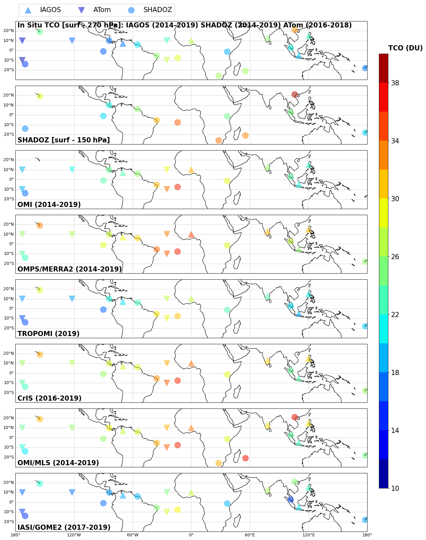
Figure 3Annual tropical tropospheric column ozone (TTCO, surface–270 hPa) from in situ data (IAGOS, SHADOZ between 2014 and 2019, and ATom between 2016 and 2018) (top panel) and TTCO (surface–150 hPa) from SHADOZ (second panel) between 2014 and 2019, as well as from OMI (surface to 100 hPa, 2014–2019), OMPS/MERRA-2 (surface to potential temperature at 380 K, 2014–2019), TROPOMI (surface to 270 hPa, 2019), CrIS (surface to 2016–2019), OMI/MLS (surface to thermal tropopause, 2014–2019), and IASI/GOME2 (surface to 12 km, 2017–2019).
Qualitatively, the mid- to upper-tropospheric ozone maximum above the Atlantic and Africa is well known (Fishman and Larsen, 1987; Thompson et al., 2003) and explained by subsidence of air masses rich in ozone (Krishnamurti et al., 1996; Thompson et al., 2000, 2003), emissions of lightning NOx (LiNOx; Sauvage et al., 2007a, b), emissions of CO VOCs (volatile organic compounds) from biomass burning (Ziemke et al., 2009; Bourgeois et al., 2021), and urban emissions (Tsivlidou et al., 2023). Hanoi, at the northern edge of our domain, shows previously documented large ozone enhancements (Ogino et al., 2022), equivalent to those above Africa and the Atlantic. A new maximum, equivalent to that found above Africa, is now detected over India, mostly related to human activities (fossil fuel combustion and agriculture burning) (Singh and Chauhan, 2020).
However, the accurate quantification of TTCO remains a challenge. The following section quantifies the differences between the satellite and in situ data in order to improve the accuracy of TTCO estimates from space.
3.3 How do the current tropospheric ozone satellite records perform?
The overall satellite biases of TTCO against in situ TTCO from IAGOS, ATom, and SHADOZ are shown in Fig. 4. All satellite TTCO values show an expected positive offset since the top level of the satellite TTCO lies higher than that of the in situ data, except for TROPOMI and IASI/GOME2. The mean differences vary from 0 to 9 DU. Figure 4 shows a mean TTCO bias of 2 DU for TROPOMI and no TTCO bias for IASI/GOME2. For TROPOMI and IASI/GOME2, showing the lowest TTCO biases, the sign of the differences can change with location (Fig. S18). TROPOMI shows positive TTCO biases of 1–4 DU from the Pacific to Africa and negative biases of 1–2 DU above India as well as Indonesia and Malaysia. IASI/GOME2 also shows negative TTCO biases of 1–5 DU above India and Indonesia–Malaysia. When using only SHADOZ data, rather than all three in situ datasets, as a reference for the TTCO from the surface to 270 hPa (Fig. S19), the mean biases remain the same (compared to Fig. 4), whereas the correlation coefficient and the mean normalized biases increase.
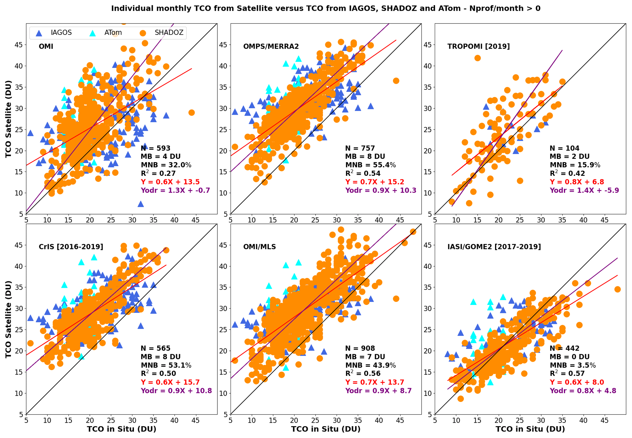
Figure 4Scatter plot of the monthly TTCO from OMI, OMPS/MERRA-2, TROPOMI, CrIS, OMI/MLS, and IASI/GOME2 satellite records compared with the in situ TTCO from IAGOS (dark blue triangles), ATom (cyan triangles), and SHADOZ (orange circles) between 2014 and 2019. The in situ TTCO values are calculated between the surface and 270 hPa. The TTCO for all satellite data extends much higher (typically up to 100–150 hPa), except for TROPOMI (TTCO calculated from the surface up to 270 hPa) and IASI/GOME2 (TTCO up to 12 km or up to 200 hPa) (Fig. S1). The linear least-squares regression is shown in red. The linear orthogonal distance regression is indicated in purple. The number of points (N), the mean biases (MB), the mean normalized biases (MNBs), and the correlation coefficient (R2) are shown in black. N corresponds to the number of months with both in situ and satellite data multiplied by the number of IAGOS regions, ATom regions, and SHADOZ sites over the time period 2014–2019.
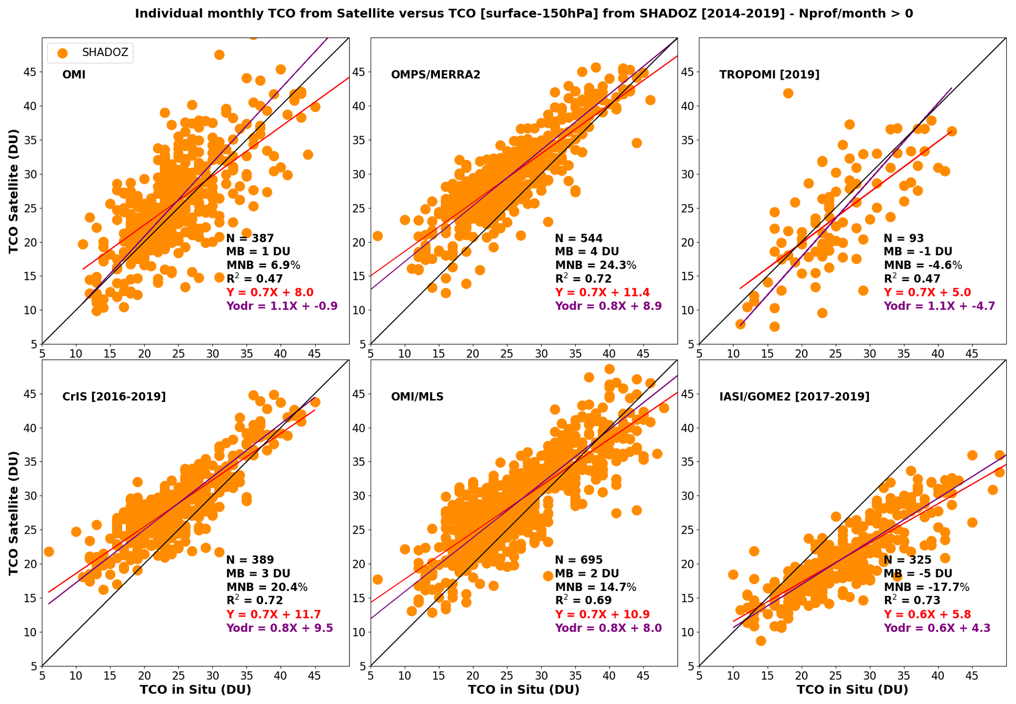
Figure 5Same as Fig. 4 but for satellite data compared with SHADOZ TTCO integrated between the surface and 150 hPa.
Because four satellite records (OMI, OMPS/MERRA-2, CrIS, and OMI/MLS) show TTCO from the surface to 100–150 hPa, altitudes that the IAGOS aircraft do not reach, we compare them to SHADOZ TTCO from the surface to 150 hPa (Fig. 5). Both the biases and the correlation coefficients improve when compared to results for TTCO up to 270 hPa, except for IASI/GOME2 for which the bias became negative (−5 DU). These results illustrate that differences in the definition of the top level of the tropospheric column play an important role in observed differences between satellite TTCO and in situ TTCO ozone data. There is hence a need for a common tropospheric column definition to make satellite TTCO estimates comparable among each other and with in situ data.
Looking at the SHADOZ sites individually (Fig. S20), the biases became closer to zero above Ascension Island (tropical Atlantic) and Natal (Brazil) when the top level of the column was changed from 270 to 150 hPa. However, the satellite TTCO records with the top level of the column higher than 270 hPa (all satellites except TROPOMI and IASI/GOME2) still overestimate TTCO after changing the reference SHADOZ TTCO's top level from 270 to 150 hPa.
The biases of TROPOMI reported in Figs. 4, S11, and 5 are in the range of those reported in Hubert et al. (2021) with a bias of 2.3 ± 1.9 DU when compared with the SHADOZ ozonesondes. Biases estimated for TROPOMI and IASI/GOME2 using the three in situ TTCO datasets from the surface to 270 hPa (Fig. 4), and biases estimated for OMI, OMPS/MERRA-2, CrIS, and OMI/MLS using SHADOZ TTCO from the surface to 150 hPa (Fig. 5), are applied to improve the accuracy of estimates of the tropospheric ozone burden (TOB), as described in Sect. 3.5.
3.4 Ozone changes with time
The estimation of trends of tropospheric ozone in the tropics based on in situ observations is a difficult task as the data are sparse in time and space, as discussed below. In this study, the Americas, Africa, Southeast Asia, and Malaysia and Indonesia are regions sampled both by IAGOS and SHADOZ, allowing us to improve the trend estimates in the free troposphere (above 700 hPa) by fusing both datasets to achieve a greater sample size and a better representation of regional ozone variability (Sects. 2.5, S1, Figs. S2–S3 and S12–S14). Figure 6 shows trends from the fused datasets. We observed increasing ozone levels between 1994 and 2019 over the Americas (trends ranging from to 1.8±0.7 nmol mol−1 decade−1 with the vertical levels), Africa (from to 7.4±0.4 nmol mol−1 decade−1), India (from 0.9±1.4 to 11±2.4 nmol mol−1 decade−1), Southeast Asia (from 2.5±0.4 to 5.1±0.8 nmol mol−1 decade−1), and Malaysia and Indonesia (from 0.5±0.6 to 8.0±0.8 nmol mol−1 decade−1). In the boundary layer (<700 hPa), local air masses sampled above SHADOZ sites and IAGOS airports are likely very different in terms of emissions, photochemistry, and air mass history, which may explain higher differences between the fused and IAGOS trends than in the free troposphere (Fig. S21). The strongest trend we find is 12.5±2.2 nmol mol−1 decade−1 in the boundary layer over Malaysia and Indonesia using IAGOS data only (Fig. S21). Malaysia–Indonesia is the region for which the number of years with missing IAGOS data is excessive (Fig. S14). As shown by Gaudel et al. (2020), the “L” shape of the trends, with a rather constant trend above the 700 hPa level and larger trends in the boundary layer, is common to the studied tropical regions except for Southeast Asia, which shows similar trends in both the boundary layer and in the free troposphere. Taking the fused trends as the reference, we find that the trends estimated using IAGOS data only tend to be overestimated by 1–2 nmol mol−1 decade−1 at 700–500 hPa, except over the Americas, and underestimated by 0.5–1 nmol mol−1 decade−1 at 500–250 hPa, except over Malaysia and Indonesia. Only IAGOS ozone profiles are available over India, and the trends in this region can reach up to 6.7±1.8 nmol mol−1 decade−1 at 350 hPa, which exceed the trends over the other regions at the same vertical level.
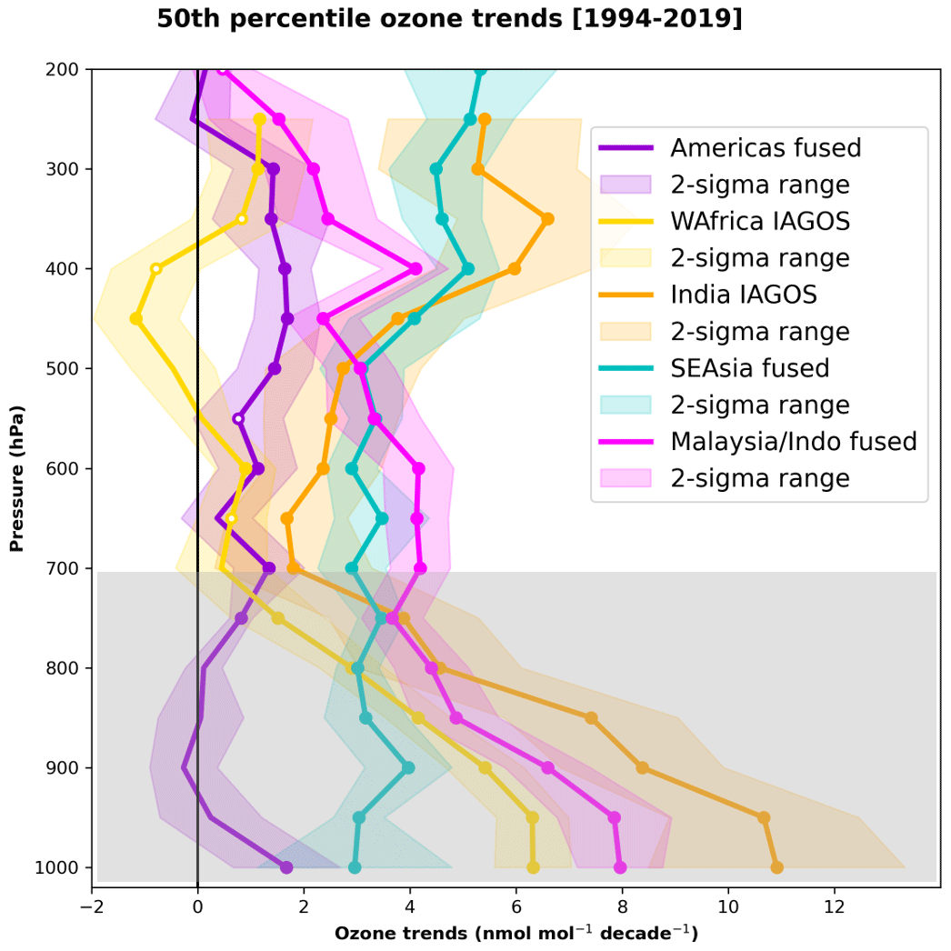
Figure 6Vertical profiles of ozone trends (nmol mol−1 decade−1) between 1994 and 2019 at 50 hPa vertical resolution. Trends are calculated for the five IAGOS regions in the tropics: the Americas, western Africa, India, Southeast Asia, and Malaysia and Indonesia. SHADOZ data are available for three out of the five IAGOS regions and used to produce fused trends (IAGOS + SHADOZ). Filled circles indicate trends with p values less than 0.05. Open circles indicate trends with p values between 0.05 and 0.1. The zero-trend value is indicated with a vertical black line. The vertical range below 700 hPa is shaded gray to indicate that the fused trends are based on several sites and airports influenced by different local air masses. The 2σ values associated with the ozone trends are shown in shaded colors.
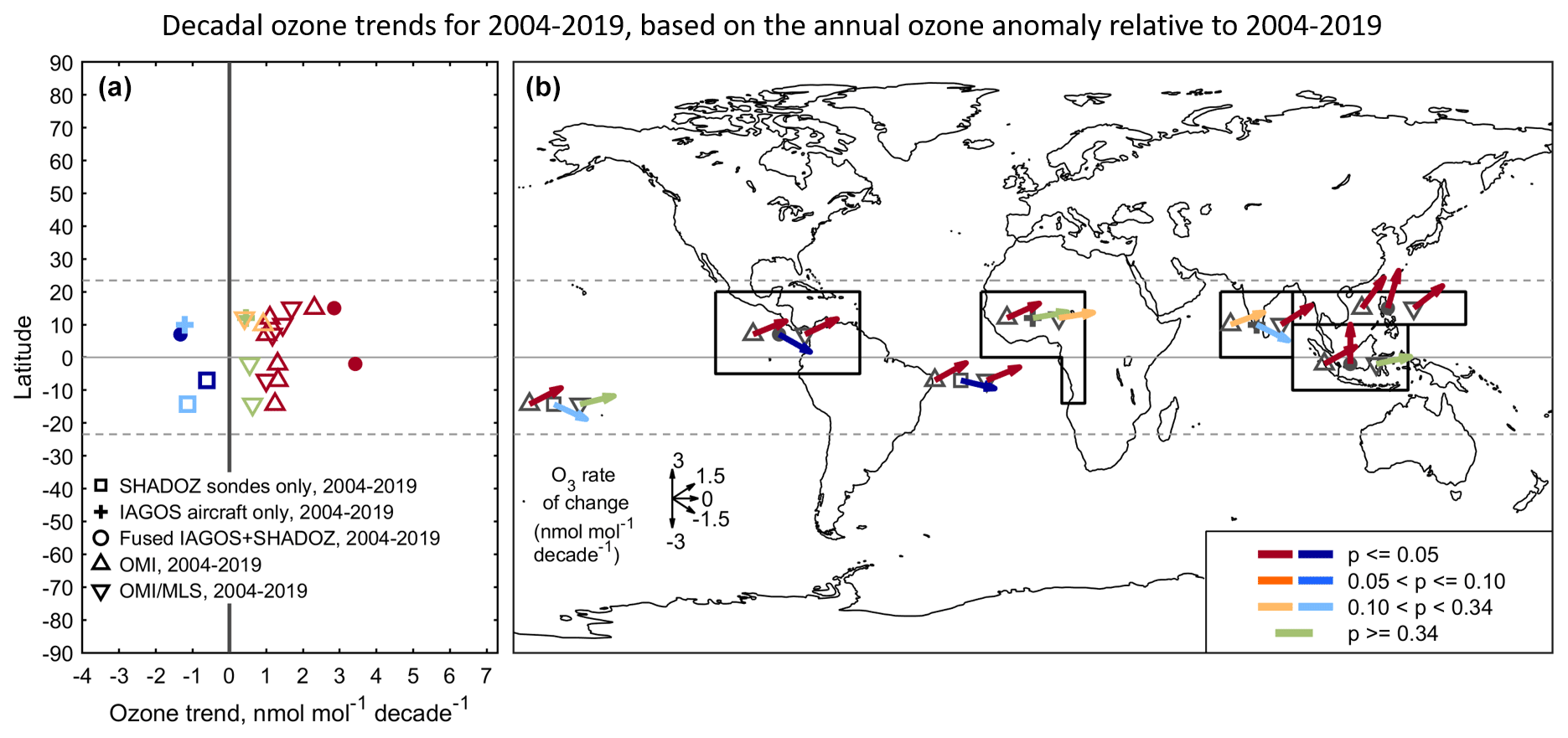
Figure 7TTCO trends (nmol mol−1 decade−1) between 2004 and 2019 from IAGOS (crosses), SHADOZ (squares), IAGOS fused with SHADOZ (circles), OMI (triangles up), and OMI/MLS (triangles down) above the five continental IAGOS regions (Americas, Africa, India, Southeast Asia, and Malaysia and Indonesia) and two oceanic SHADOZ regions (Samoa and Natal + Ascension Island). Panel (a) shows the trends of ozone as a function of latitude. Panel (b) shows the trends of ozone on the map with the black rectangles demarcating the five IAGOS regions. On the map, the longitude of the crosses, circles, triangles, and squares are arbitrary and the latitude is the mean latitude of the black rectangles or relative to the SHADOZ sites. The direction of the arrows shows the magnitude of the trends and the colors indicate the p value. The TTCO trends from in situ data are calculated from the monthly TTCO between the surface and 100 hPa, except over India where IAGOS profiles are available between the surface and around 200 hPa. The TTCO trends from OMI and OMI/MLS are calculated from the monthly TTCO defined between the surface and around 102–105 hPa (Fig. S1).
Satellite data from OMI are available continuously since 2004 and 15-year trends can now be estimated. The interannual variability of the TTCO from satellite and in situ data is shown in Fig. S22. Several time series of the monthly mean of tropospheric ozone above Malaysia and Indonesia show the influence of climate variability such as El Niño and related fires. For example, we see a peak of ozone in September 2015, in agreement with a peak of CO emissions due to biomass burning above equatorial Asia (Fig. S23; Mead et al., 2018).
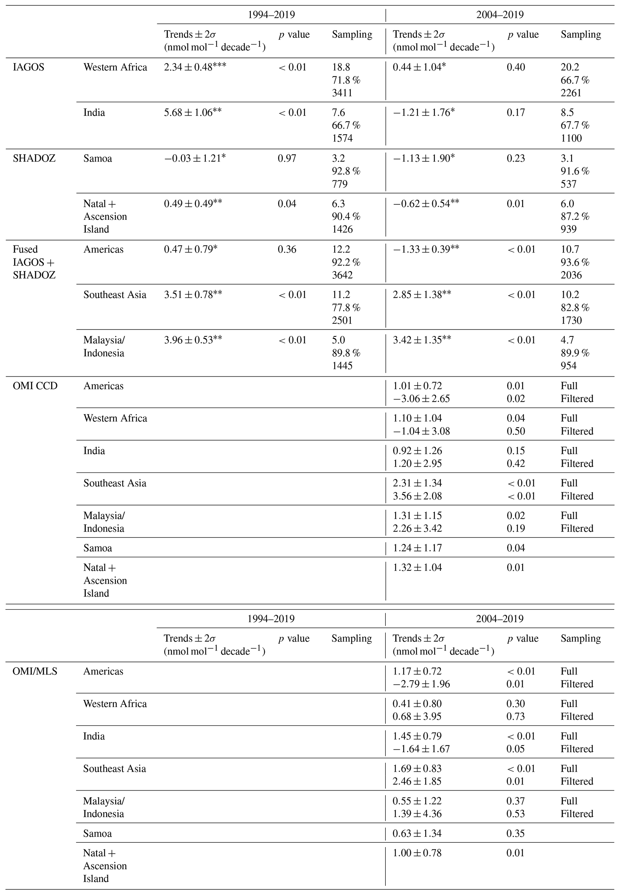
Figure 7 and Table 1 show the trend estimates of TTCO in nmol mol−1 decade−1 from OMI CCD, OMI/MLS, and in situ data between 2004 and 2019. The in situ trends between 2004 and 2019 (Fig. S24 and Table 1) are negative for Samoa ( nmol mol−1 decade−1), the Americas ( nmol mol−1 decade−1), Natal and Ascension Island ( nmol mol−1 decade−1), and India ( nmol mol−1 decade−1) and positive for western Africa (0.4±1 nmol mol−1 decade−1), Southeast Asia (2.9±1.4 nmol mol−1 decade−1), and Malaysia and Indonesia (3.4±1.3 nmol mol−1 decade−1). The presence of negative trends above some regions for the shorter 2004–2019 period differs greatly from the longer 1994–2019 time period, which had no time series with negative trends except above Samoa (Fig. 7, Table 1). They also differ from the positive trends shown by the satellite data (full record, Fig. 7, Table 1). The satellite trends vary between 0.9±1.3 nmol mol−1 decade−1 over India and 2.3±1.3 nmol mol−1 decade−1 over Southeast Asia with OMI and between 0.4±0.8 nmol mol−1 decade−1 over western Africa and 1.7±0.8 nmol mol−1 decade−1 over Southeast Asia with OMI/MLS (Fig. 7, Table 1).
Discrepancies between satellites and in situ observations in assessing trends may be caused by (i) the different definitions of the tropospheric column (100 or 200 hPa or tropopause defined with the temperature lapse rate), (ii) the diminished sensitivity of the space-based instruments in the boundary layer, or (iii) the limited data availability and relatively short record that may lead to less accurate and precise trends (Figs. S2 and S3). In particular, we highlight previous research that has demonstrated the difficulty in detecting ozone trends in time series that are noisy and/or sparsely sampled (Weatherhead et al., 1998; Fischer et al., 2011; Barnes et al., 2016; Fiore et al., 2022). These studies show that 20 years of observations, or more, are needed for trend detection and that model ensembles (based on differing initial conditions) can produce trends for a given location that vary so widely that even the sign can fluctuate between positive and negative when dealing with time periods shorter than 20 years. Furthermore, previous studies of in situ ozone profiles concluded that a sampling frequency of once per week generally fails to produce accurate monthly mean and trend values (Logan, 1999; Saunois et al., 2012; Chang et al., 2020, 2022). Consistent with these previous studies, we conducted our own analysis of tropical ozone time series (see the Sect. S1) and found that these sparsely sampled datasets have very low signal-to-noise ratios, which makes trend detection very difficult, especially when a time series is less than 20 years in length (Chang et al., 2020, 2022). The comparison between the in situ and satellite trends is only 15 years in length (2004–2019), and the in situ datasets are sparsely sampled, characteristics consistent with known challenges for trend detection. Furthermore, we point out that the robustness of the positive trends from the satellite records is greatly diminished, and even becomes undetectable, when we reduce the sample size of the satellite data in the IAGOS regions to match the sparse sampling frequency of the aircraft observations (Fig. S25). For example, when the satellite data are fully sampled across the five IAGOS domains, all trends are positive, within the range 0.4±0.8 to 2.3±1.3 nmol mol−1 decade−1. But when the satellite sample sizes are reduced so that they only coincide with the specific months and grid cells sampled by the IAGOS aircraft, the range of the trends more than doubles and even includes negative values ( to nmol mol−1 decade−1). This increased uncertainty is an expected outcome of decreased sampling frequency, as illustrated in Fig. S2.
The color scheme in Table 1 reflects our overall confidence in the presence of in situ trend estimates, according to the number of missing monthly values, monthly average data availability, the length of study period, and the p value of the trend estimate (the trends are confident only if a low p value and high data coverage are met; see Appendix A for further details and Sect. S3 for a discussion of the confidence assigned to each region). When assigning a level of confidence to a trend we weigh the p value and the data coverage and ask the following question: are we confident that a positive or negative trend is reliable? For example, if a positive trend has a low p value but also low data coverage then our confidence that the trend is reliable is diminished. Western Africa is the only region in this study with sufficient sampling for reliable trend detection with high confidence (1994–2019). Trends derived from the other in situ time series only have low or medium confidence due to sampling deficiencies and/or low estimation certainty (based on the p value). When we compare the satellite trends to the in situ trends we find that they are consistent for Southeast Asia, with all three datasets showing positive trends. In the other regions we find discrepancies between the in situ and satellite trends, but in these regions, we do not have high confidence in the in situ trends, and therefore there is no reason to reject the satellite trend values, which generally indicate an increase in ozone in the study regions. However, the discrepancies between satellite and in situ trends in the Americas and Natal + Ascension Island are nuanced and require further discussion. In the region of the Americas we assigned medium confidence to the decreasing ozone trends based on the in situ observations, which contrasts strongly with the clear positive trends based on the satellite data. When we reduced the satellite sampling coverage to match the locations and months with IAGOS observations, we found that the satellite trends switched from clear positive trends to clear negative trends (Fig. S25). This exercise indicates that the available in situ observations are not representative of the large region, and therefore they do not provide sufficient justification for rejecting the positive trends reported by the satellite data. In situ ozone trends above Natal + Ascension Island have a weak negative trend ( nmol mol−1 decade−1) with medium confidence, while the satellite trends show weak positive trends. While the divergence between the positive and negative trends is small over this short time period (2–3 nmol mol−1 over 15 years), this discrepancy warrants further investigation to determine the differences between the satellite and in situ time series trends.
3.5 Comparison to previous studies
Using the ozonesondes from the SHADOZ network, Thompson et al. (2021) found positive annual trends of about 1.2±3 % decade−1 to 1.9±3 % decade−1 (0.08±1.68 nmol mol−1 decade−1 to 0.78±1.66 nmol mol−1 decade−1) between 1998 and 2019 at 5–10 km (∼ 500–250 hPa) across the tropical belt. They reported maximum trends (1.9±3 % decade−1) above Malaysia and Indonesia (Kuala Lumpur + Java) as well as the Americas (San Cristóbal + Paramaribo) and minimum trends (1.2±3 % decade−1) above Africa (Nairobi). The SHADOZ trends are slightly lower than the IAGOS + SHADOZ fused trends or IAGOS trends, which may be explained by the different starting points of the time series (1998 for SHADOZ data and 1994 for IAGOS data), but they are all positive.
Previous studies of TTCO trends from satellite data relied on data harmonization in order to combine several satellite records into a time series spanning at least 2 decades and to better account for the climate variability in the trend estimates (Heue et al., 2016; Leventidou et al., 2018; Ziemke et al., 2019; Pope et al., 2023). Heue et al. (2016) found a tropical trend of 0.7±0.12 DU decade−1, with regional trends ranging from +1.8 DU decade−1 on the African Atlantic coast to −0.8 DU decade−1 over the western Pacific Ocean. Leventidou et al. (2018) reported positive trends of TTCO of 1 to 1.5 DU decade−1 between 1996 and 2015 over northern South America, North Africa, southern Africa, and India and negative trends of −1.2 to −1.9 DU decade−1 above the oceans (Pacific, Atlantic, Indian oceans). Using TOMS–OMI/MLS, Ziemke et al. (2019) reported positive trends between 1979 and 2016 across the tropical latitude band 20° S–20° N except above the southeastern tropical Pacific Ocean and southeastern Indian Ocean. The highest positive trends (up to 1.3 DU decade−1) were found above South–Southeast Asia and central Africa. Finally, a new harmonized product that quantifies ozone between the surface and 450 hPa reports much higher tropical trends than the other studies, with increases of 2.9±1.6 DU decade−1 for the southern tropical band (0–15° S) and 3.9±1.8 DU decade−1 for the northern tropical band (0–15° N) for the years 1996–2017 (Pope et al., 2023). While these findings vary regarding the magnitude of trends in the tropics, when taken into consideration with the 1994–2019 in situ trends reported by the present study, the preponderance of evidence indicates a general increase in TTCO since the mid-1990s.
Wang et al. (2022) report an increase in TTCO (950–250 hPa) trends using the GEOS-Chem chemical transport model above the IAGOS regions and SHADOZ sites between 1995 and 2017, except above Samoa. The trends vary with location between nmol mol−1 decade−1 above Samoa and 2.87±0.23 nmol mol−1 decade−1. In general, they find that the TTCO trends from the model are lower by 1–3 nmol mol−1 decade−1 than from the observations, except above Paramaribo.
Table 1Summary of the TTCO trends in nmol mol−1 decade−1 from IAGOS, SHADOZ, OMI/MLS, and OMI CCD. The sampling column reports three numbers for the in situ data: (i) the number on the top refers to the average number of profiles per month taking into account all the months with profiles, (ii) the number in the middle refers to the percentage of months with data for the studied time period (1994–2019 or 2004–2019), and (iii) the number on the bottom refers to the total number of profiles for the studied time period (1994–2019 or 2004–2019). For the satellites, the sampling column reports “full” when the full record is taken into account and “filtered” when the satellite sample sizes have been greatly reduced so that they only coincide with the specific months and grid cells sampled by the IAGOS aircraft. In the table we indicate when the ozone trends from the in situ data are characterized with low confidence (*), medium confidence (), and high confidence () based on the sampling and the p value.
3.6 Tropical tropospheric ozone burden
Figure 8 shows the time series of the tropical tropospheric ozone burden (TTOB, Tg) from six satellite records. As described in the Methods section, OMI/MLS, OMI CCD, OMPS/MERRA-2, TROPOMI, CrIS, and IASI/GOME2 are sampled in the 20° S–20° N latitude band. For both hemispheres we find two distinguished groups in terms of TTOB (Fig. 8, panels a and c): (i) TROPOMI and IASI/GOME2 with a range of TTOB of 35–45 Tg and (ii) OMI/MLS, OMPS/MERRA-2, and CrIS with a range of TTOB of 40–65 Tg. These differences are explained by the difference of the upper bound of the tropospheric column (lower for TROPOMI and IASI/GOME2 than for the other satellite data). OMI CCD TTOB (35–55 Tg) falls between these two groups. The seasonal variability of TTOB is lower in the Northern Hemisphere than in the Southern Hemisphere.
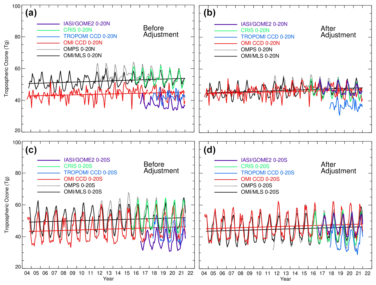
Figure 8Time series of tropospheric ozone burden (Tg) from OMI/MLS, OMPS/MERR2, OMI CCD, TROPOMI, CrIS, and IASI/GOME2. The panels show the monthly means for the Northern Hemisphere (a, b) and the Southern Hemisphere (c, d) before and after bias correction. The biases we used are in Dobson units (DU) and from the differences between IASI/GOME2 and TROPOMI TTCO using the reference TTCO up to 270 hPa and between OMI, OMI/MLS, OMPS/MERRA-2, CrIS, and TTCO using the reference TTCO up to 150 hPa (Figs. 4 and 5).
The biases calculated from the scatter plots of satellite versus ozonesondes (Figs. 4 and 5) are used to correct the satellite time series. The adjustment reduced the differences by about 10 Tg in the Northern Hemisphere and by 5 Tg in the Southern Hemisphere between the two groups mentioned above. After adjustment, OMI CCD TTOB become close to (Northern Hemisphere) or higher than (Southern Hemisphere) OMI/MLS TTOB. In the Northern Hemisphere, after adjustment (Fig. 8, panels b and d, and Table 2), TROPOMI TTOB (30–40 Tg) is lower than for the other datasets (40–55 Tg). In the Southern Hemisphere, it is difficult to distinguish the two groups after adjustment. TROPOMI TTOB (30–48 Tg) shows lower values than the other datasets (30–60 Tg) but the average differences are smaller than in the Northern Hemisphere.
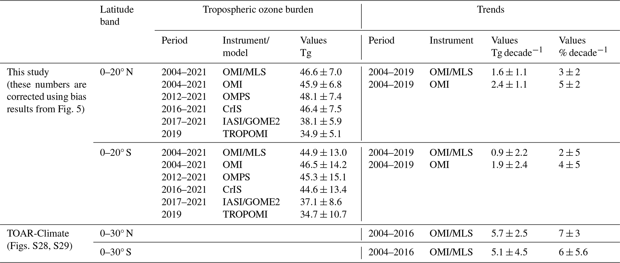
Table 2 summarizes TTOB trends from this study and from TOAR-Climate (Gaudel et al., 2018). Trends are positive and higher in the Northern Hemisphere (1.6±1.1 to 5.7±2.5 Tg decade−1) than the Southern Hemisphere (0.9±2.2 to 5.1±4.5 Tg decade−1). Because TTOB trends in Tg decade−1 can increase with the width of the latitude band (assuming trends are all positive across the range of latitudes considered), we also report trends in % decade−1 to compare trends between different latitude bands. The 2004–2016 OMI/MLS trends in the 0–30° north and south latitude bands are higher by a factor of 3 or 5 than the 2004–2019 OMI/MLS trends in the 0–20° north and south latitude bands. These differences might be explained by the influence of the larger increases in subtropical tropospheric ozone.
Table 2Summary of tropical tropospheric ozone burden values and trends.
Long and midterm records of tropospheric ozone from IAGOS, SHADOZ, and OMI, as well as new observations from the ATom aircraft campaign and the CrIS and IASI/GOME2 satellite instruments, are now available in the tropics, a region undergoing rapid changes in terms of human activity and emissions of ozone precursors. The present study takes advantage of these new data records to assess the distribution of tropical tropospheric ozone, and it uses the longest records to assess its trends.
Present-day distribution
-
With greater availability of ozone profiles across the tropics we can now demonstrate that southern India is among the most polluted regions (western Africa, tropical South Atlantic, Southeast Asia, Malaysia and Indonesia), with 95th percentile ozone values reaching 80 nmol mol−1 in the lower free troposphere, comparable to midlatitude regions, such as northeastern China and Korea – Sect. 3.1, Fig. 2.
-
The lowest ozone values (5th percentile) are less than 10 nmol mol−1 and are observed by SHADOZ and ATom in the boundary layer (below 700 hPa) above the Americas and the tropical South Pacific – Sect. 3.1, Fig. 2.
-
From space, the distribution of tropical tropospheric column ozone (TTCO) ranges from 10 to 40 DU in the 20° S–20° N latitude band – Sect. 3.2, Fig. 3.
-
The definition of the tropospheric column plays an important role in assessing tropical tropospheric ozone. Satellite data with a higher upper limit overestimate tropical column ozone compared to in situ data. Mean biases reach up to 9 DU for OMPS/MERRA-2 when compared to IAGOS, ATom, and SHADOZ. The bias is 0 for IASI/GOME2 for which the column definition matches the in situ observations – Sect. 3.3, Fig. 4
-
The smallest biases (≤2 DU) are found when matching the top limit of the in situ profiles to that of the OMI, TROPOMI, and IASI/GOME2 satellite records – Sect. 3.3, Figs. 4 and 5.
-
The in situ observations were critical for adjusting the biases in the satellite products, bringing them into closer alignment. In the 20° S–20° N latitude band, the tropical tropospheric ozone burden (TTOB) is slightly larger in the Northern Hemisphere (between 34.9±5.1 and 48.1±7.4 Tg) than in the Southern Hemisphere (between 34.7±10.7 and 46.5±14.2 Tg). The seasonal variability of TTOB is lower in the Northern Hemisphere than in the Southern Hemisphere – Sect. 3.6, Fig. 8, and Table 2.
Trends
-
When focusing on the longest available records exceeding 20 years (1994–2019, IAGOS/SHADOZ data reported in this study) or 30 years (1979–2016 satellite record reported by Ziemke et al., 2019) we see a consistent picture of increasing ozone across the tropics. IAGOS and SHADOZ data were fused to increase the sample sizes and to improve the statistics of the data over three out of the five IAGOS regions: the Americas, Southeast Asia, and Malaysia and Indonesia (western Africa and India with no SHADOZ data). India and Malaysia–Indonesia are the regions with the strongest ozone increase below 800 hPa (11±2.4 and 8±0.8 nmol mol−1 decade−1 close to the surface, respectively) and India above 400 hPa (up to 6.8±1.8 nmol mol−1 decade−1). Southeast Asia and Malaysia–Indonesia show the highest increase in the mid-troposphere (550–750 hPa, up to 3.4±0.8 and 4±0.5 nmol mol−1 decade−1, respectively). Trends of the tropical tropospheric column ozone reflect these results. In terms of in situ trend reliability based on data availability and the p value of the trend estimate, we have the most confidence in western Africa (while it is still not ideal due to moderate data gaps) and the least confidence in Samoa and the Americas – Sect. 3.4, Fig. 6.
-
For shorter time periods (<20 years) trend detection can be even more challenging due to the larger additional uncertainty associated with sparsely sampled ozone records – Sect. 3.4, Figs. 7, and S24.
-
The OMI and OMI/MLS satellite records have a very high sampling frequency compared to the sparse in situ datasets and mostly show positive 15-year (2004–2019) trends above the IAGOS regions (from 0.55±1.22 to 2.31±1.34 nmol mol−1 decade−1), with the maximum trends over Southeast Asia of 2.31±1.34 nmol mol−1 decade−1 with OMI CCD and 1.69±0.89 nmol mol−1 decade−1 with OMI/MLS. The strongest agreement between satellite and in situ trends is found above Southeast Asia where TTCO had increased at a rate of about 2–3 nmol mol−1 decade−1. These trends are consistent with the results from Ziemke et al. (2019) using TOMS–OMI/MLS records and Gaudel et al. (2020) using IAGOS ozone profiles. Above the other regions, we only have low to medium confidence in the in situ trends; therefore, we concluded that we have no reason to reject the positive tropical tropospheric ozone trends based on satellite data. However, the discrepancy between the weak positive satellite trends and the weak negative in situ trends above Natal + Ascension Island warrants further investigation – Sect. 3.4 and 3.5, Fig. 7, and Table 1.
This study demonstrates that most tropical regions require increased and/or continuous sampling (in situ and remote sensing) of ozone because either there are no data or the data are so sparse that it is difficult to estimate accurate and precise trends to evaluate the satellite records. However, we also demonstrate that the current sampling frequency is adequate for bias-correcting the satellite products, as shown in Fig. 8.
TROPOMI, IASI/GOME2, CrIS, and OMPS/MERRA-2 are recently available satellite records, and their overlap for several years with the OMI record will ensure the continuity of ozone and precursor observations from space when the NASA Aura mission terminates by 2025. GEMS, the only geostationary mission covering the tropics (tropical Asia), will bring new capabilities in monitoring the region with the strongest ozone increases in the world, with higher spatial and temporal resolution than polar-orbiting instruments.
This study underscores the importance of harmonizing TTCO data records such that they have a common vertical top level of the tropospheric column. Additionally, there is a pressing need for common profile retrieval schemes for different nadir sensors, such as those provided by initiatives like TROPESS (TRopospheric Ozone and its Precursors from Earth System Sounding, https://tes.jpl.nasa.gov/tropess/, last access: 22 August 2023).
Moreover, to better understand the drivers behind the observed increases in TTOB, it is essential to conduct simulations using global chemical transport models, chemistry–climate models, Earth system models, and regional models spanning recent decades.
Encouragingly, these endeavors have been newly proposed within the framework of the Tropospheric Ozone Assessment Report phase II (TOAR-II), an initiative under the International Global Atmospheric Chemistry (IGAC) project. These efforts will be the focus of forthcoming publications featured in the TOAR-II Community Special Issue.
It is also worth noting that the TOAR-II Community Special Issue will include similar trend analyses applied at the global scale using IAGOS, ozonesondes, FTIR, and Brewer–Dobson (Umkehr) data.
The Intergovernmental Panel on Climate Change (IPCC) developed a guidance note for the consistent treatment of uncertainties (Mastrandrea et al., 2010) that was followed by the fifth and sixth IPCC assessment reports. Among other applications, the calibrated language described by the guidance note is helpful for the discussion of long-term trends and for communicating the level of confidence that an author team wishes to assign to a particular trend value or to an ensemble of trend values. Confidence in the validity of a finding is expressed qualitatively with five qualifiers (very low, low, medium, high, and very high) based on the type, amount, quality, and consistency of the available evidence, as well as the level of agreement among studies addressing the same phenomenon (see Fig. 1 of Mastrandrea et al., 2010).
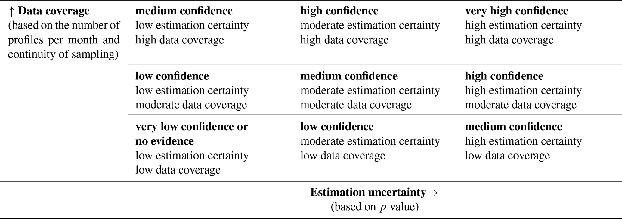
Table A1Calibrated language for discussing confidence in long-term trend estimates based on ozone profiles. Data coverage refers to the number of ozone profiles in a month and the number of months with available data. Estimation uncertainty refers to the uncertainty of a trend line drawn through monthly means, as quantified by the p value and the 95 % confidence interval.
Following IPCC, the Tropospheric Ozone Assessment Report (TOAR) developed its own guidance note on best statistical practices for TOAR analyses, featuring an uncertainty scale for assessing the reliability and likelihood of the estimated trend (Chang et al., 2023). The uncertainty scale has five qualifiers as follows: very low certainty or no evidence, low certainty, medium certainty, high certainty, and very high certainty. Each qualifier corresponds to a range of values associated with either the signal-to-noise ratio or the p value of the trend. A limitation of the uncertainty scale is that it is best suited for surface ozone time series with high-frequency sampling, which allows for robust calculation of monthly means, upon which the trends are calculated. For the case of calculating trends based on sparse ozone profiles, in many cases the monthly means are biased or unreliable due to low sampling frequency, which adds additional uncertainty to the calculation of the trend. Because the p value (or the signal-to-noise ratio) of a trend based on monthly means does not consider the impact of low sampling frequency on the monthly means, we developed new calibrated language to express our confidence in trends based on sparse ozone profiles.
Following the methodology of IPCC (Mastrandrea et al., 2010) Table A1 presents a confidence scale that we use in this present study to express our confidence in a trend based on sparse ozone profiles (as reported in Table 1 in the main text). Any line fit though a time series will produce a trend value that is either positive or negative, and we use this scale to answer the following question: are we confident that a positive or negative trend is reliable? The confidence scale considers both data coverage (based on the number of profiles per month and continuity of sampling) and the estimation of the uncertainty of the trend based on the p value and the 95 % confidence interval. Higher confidence can be placed on trends with lower p values and greater data coverage, while less confidence is placed on trends with relatively high p values and low data coverage. The selection of a particular confidence level is qualitative, with no sharp boundaries; however, the following guidelines inform our decision-making.
Data coverage. Previous studies (Logan, 1999; Saunois et al., 2012; Chang et al., 2020) have shown that sampling rates of once per week (or less) fail to provide accurate monthly means, while increased sampling rates of two or three times per week are more accurate. The most accurate sampling rate is four times per week or higher. Continuous data records with no, or limited, gaps are more reliable than records with multiple or large gaps. Data length also plays a role in trend reliability. A time series with more than 90 % of months with data and with more than 15 profiles per month is considered to have high data coverage. A time series with 66 % to 90 % of months with data and with 7–15 profiles per month is considered to have moderate data coverage (this also applies to a region that only meets one condition for high data coverage). A time series that has less than 66 % of months with data or fewer than seven profiles per month has low data coverage. It should be noted that, based on our criteria, none of the current study regions meet the criteria for high data coverage, and therefore the top row in Table A1 is not applicable to this study. In addition, since we derive the trends based on either a 25-year or a 15-year record, it is natural to consider the trends derived from a longer data record as more robust, as a record length less than 2 decades is generally insufficient to eliminate the impact of interannual variability (Weatherhead et al., 1998; Barnes et al., 2016; Fiore et al., 2022). Therefore, all of the time series in Table 1 with 15-year records are considered to have low data coverage.
Estimation uncertainty. In general, lower p values and higher signal-to-noise ratios are indicators of a robust trend. The “Guidance note on best statistical practices for TOAR analyses” (Chang et al., 2023) assigns the following degrees of certainty according to p value: very high certainty (p≤0.01), high certainty (), medium certainty (), low certainty (), and very low certainty or no evidence (p>0.33). We acknowledge that the trend calculation does not consider the inherent quality of the data (i.e., accuracy and precision of the data), which will be explored in future studies within TOAR Phase II.
The monthly quasi-biennial oscillation values can be found at https://www.geo.fu-berlin.de/met/ag/strat/produkte/qbo/qbo.dat (Freie Universitat Berlin, 2024). The monthly El Niño–Southern Oscillation index can be found at https://psl.noaa.gov/enso/mei/ (NOAA PSL, 2024). ATom data are archived at https://daac.ornl.gov/ATOM/guides/ATom_merge.html and are published through the Distributed Active Archive Center for Biogeochemical Dynamics (Wofsy et al., 2018). IAGOS ozone profiles can be found at https://iagos.aeris-data.fr/ (AERIS/IAGOS, 2024). SHADOZ ozone profiles can be found at https://tropo.gsfc.nasa.gov/shadoz/ (SHADOZ, 2024). IASI+GOME2 satellite data can be found at https://iasi.aeris-data.fr/o3_iago2/, last access: 8 February 2023 (AERIS/IASI, 2024). OMI CCD, OMI/MLS and OMPS/MERRA-2 can be found at https://acd-ext.gsfc.nasa.gov/Data_services/cloud_slice/ (NASA, 2024a). TROPOMI CCD can be found at the NASA EarthData repository: https://disc.gsfc.nasa.gov/datasets?keywords=tropomi&page=1 (NASA, 2024b). CrIS can be found at https://disc.gsfc.nasa.gov/ (NASA, 2024c) (see the Methods section for more details on the data preprocessing). The fused datasets and trends (including uncertainty and p value associated with the trend estimate, as well as fitted coefficients for ENSO and QBO in Eq. 1 of Sect. 2.5) can be found at https://csl.noaa.gov/groups/csl4/modeldata/ (NOAA CSL/Chang K.-l., 2024).
The supplement related to this article is available online at: https://doi.org/10.5194/acp-24-9975-2024-supplement.
Conception and design of the study: AG, IB, ML, KLC, and ORC. Generation, collection, assembly, analysis, and/or interpretation of data: AG, IB, ML, KLC, ORC, JZ, BS, AMT, RMS, DEK, NS, DH, AK, JC, KPH, PV, KA, JP, CRT, and TBR. Drafting and/or revision of the manuscript: AG, IB, ML, KLC, ORC, JP, KA, AMT, RMS, DH, AK, NS, JZ, GJF, and BCM. All authors approved the manuscript for submission.
At least one of the (co-)authors is a guest member of the editorial board of Atmospheric Chemistry and Physics for the special issue “Tropospheric Ozone Assessment Report Phase II (TOAR-II) Community Special Issue (ACP/AMT/BG/GMD inter-journal SI)”. The peer-review process was guided by an independent editor, and the authors also have no other competing interests to declare.
Publisher’s note: Copernicus Publications remains neutral with regard to jurisdictional claims made in the text, published maps, institutional affiliations, or any other geographical representation in this paper. While Copernicus Publications makes every effort to include appropriate place names, the final responsibility lies with the authors.
This article is part of the special issue “Tropospheric Ozone Assessment Report Phase II (TOAR-II) Community Special Issue (ACP/AMT/BG/GMD inter-journal SI)”. It is a result of the Tropospheric Ozone Assessment Report, Phase II (TOAR-II, 2020–2024).
This research was supported by the NOAA cooperative agreement with CIRES (NA17OAR4320101 and NA22OAR4320151).
We acknowledge the support of the NOAA JPSS PGRR program.
The authors acknowledge the strong support of the European Commission, Airbus, and the airlines (Lufthansa, Air France, Austrian, Air Namibia, Cathay Pacific, Iberia, and China Airlines so far) who have carried the MOZAIC or IAGOS equipment and performed the maintenance since 1994. In its last 10 years of operation, MOZAIC has been funded by INSU-CNRS (France), Météo-France, Université Paul Sabatier (Toulouse, France), and the Jülich Research Center (FZJ, Jülich, Germany). IAGOS (https://www.iagos.org/, last access: 23 August 2024) has been additionally funded by the EU projects IAGOS-DS and IAGOSERI. The IAGOS database is supported by AERIS, the French portal for data and service for the atmosphere (see https://iagos.aeris-data.fr, last access: April 2023). SHADOZ data are provided through support of NASA's Upper Atmospheric Composition (UACO), the NOAA/Global Monitoring Division, and operators and data archivists across 20 organizations in North and South America, Europe, Africa, and Asia.
This paper was edited by Tim Butler and reviewed by two anonymous referees.
AERIS/IAGOS: IAGOS ozone profiles data [data set], https://iagos.aeris-data.fr/, last access: 23 August 2024.
AERIS/IASI: IASI + GOME2 satellite data [data set], https://iasi.aeris-data.fr/o3_iago2/, last access: 23 August 2024.
Archibald, A. T., Neu, J. L., Elshorbany, Y. F., Cooper, O. R., Young, P. J., Akiyoshi, H., Cox, R. A., Coyle, M., Derwent, R. G., Deushi, M., and Finco, A.: Tropospheric Ozone Assessment Report: A critical review of changes in the tropospheric ozone burden and budget from 1850 to 2100, Elem. Sci. Anth., 8, 034, https://doi.org/10.1525/elementa.2020.034, 2020.
Barnes, E. A., Fiore, A. M., and Horowitz, L. W.: Detection of trends in surface ozone in the presence of climate variability, J. Geophys. Res.-Atmos., 121, 6112–6129, 2016.
Blot, R., Nédélec, P., Boulanger, D., Wolff, P., Sauvage, B., Cousin, J.-M., Athier, G., Zahn, A., Obersteiner, F., Scharffe, D., Petetin, H., Bennouna, Y., Clark, H., and Thouret, V.: Internal consistency of the IAGOS ozone and carbon monoxide measurements for the last 25 years, Atmos. Meas. Tech., 14, 3935–3951, https://doi.org/10.5194/amt-14-3935-2021, 2021.
Bourgeois, I., Peischl, J., Thompson, C. R., Aikin, K. C., Campos, T., Clark, H., Commane, R., Daube, B., Diskin, G. W., Elkins, J. W., Gao, R.-S., Gaudel, A., Hintsa, E. J., Johnson, B. J., Kivi, R., McKain, K., Moore, F. L., Parrish, D. D., Querel, R., Ray, E., Sánchez, R., Sweeney, C., Tarasick, D. W., Thompson, A. M., Thouret, V., Witte, J. C., Wofsy, S. C., and Ryerson, T. B.: Global-scale distribution of ozone in the remote troposphere from the ATom and HIPPO airborne field missions, Atmos. Chem. Phys., 20, 10611–10635, https://doi.org/10.5194/acp-20-10611-2020, 2020.
Bourgeois, I., Peischl, J., Neuman, J. A., Brown, S. S., Thompson, C. R., Aikin, K. C., Allen, H. M., Angot, H., Apel, E. C., Baublitz, C. B., and Brewer, J. F.: Large contribution of biomass burning emissions to ozone throughout the global remote troposphere, P. Natl. Acad. Sci. USA, 118, e2109628118, https://doi.org/10.1073/pnas.210962811, 2021.
Buonaccorsi, J. P.: Measurement error: models, methods, and applications, CRC press, Errors of measurement in statistics, Technometrics, 10, 637–666, 2010.
Cazorla, M.: Ozone structure over the equatorial Andes from balloon-borne observations and zonal connection with two tropical sea level sites, J. Atmos. Chem., 74, 377–398, https://doi.org/10.1007/s10874-016-9348-2, 2017.
Cazorla, M., Parra, R., Herrera, E., and da Silva, F. R.: Characterizing ozone throughout the atmospheric column over the tropical Andes from in situ and remote sensing observations, Elem. Sci. Anth., 9, 00019, https://doi.org/10.1525/elementa.2021.00019, 2021a.
Chandra, S., Ziemke, J. R., and Min, W., and Read, W. G.: Effects of 1997–1998 El Niño on tropospheric ozone and water vapor, Geophys. Res. Lett., 25, 3867–3870, 1998.
Chang, K.-L., Cooper, O. R., Gaudel, A., Petropavlovskikh, I., and Thouret, V.: Statistical regularization for trend detection: an integrated approach for detecting long-term trends from sparse tropospheric ozone profiles, Atmos. Chem. Phys., 20, 9915–9938, https://doi.org/10.5194/acp-20-9915-2020, 2020.
Chang, K. L., Schultz, M. G., Lan, X., McClure-Begley, A., Petropavlovskikh, I., Xu, X., and Ziemke, J. R.: Trend detection of atmospheric time series: Incorporating appropriate uncertainty estimates and handling extreme events, Elem. Sci. Anth., 9, 00035, https://doi.org/10.1525/elementa.2021.00035, 2021.
Chang, K. L., Cooper, O. R., Gaudel, A., Allaart, M., Ancellet, G., Clark, H., Godin-Beekmann, S., Leblanc, T., Van Malderen, R., Nédélec, P., and Petropavlovskikh, I.: Impact of the COVID-19 economic downturn on tropospheric ozone trends: An uncertainty weighted data synthesis for quantifying regional anomalies above western North America and Europe, AGU Advances, 3, e2021AV000542, https://doi.org/10.1029/2021AV000542, 2022.
Chang, K.-L., Schultz, M. G., Koren, G., and Selke, N.: Guidance note on best statistical practices for TOAR analyses, https://igacproject.org/activities/TOAR/TOAR-II (last access: 23 August 2023), 2023.
Cooper, O. R., Schultz, M. G., Schröder, S., Chang, K. L., Gaudel, A., Benítez, G. C., Cuevas, E., Fröhlich, M., Galbally, I. E., Molloy, S., and Kubistin, D.: Multi-decadal surface ozone trends at globally distributed remote locations, Elem. Sci. Anth., 8, p. 23, 2020.
Craigmile, P. F. and Guttorp, P.: A combined estimate of global temperature, Environmetrics, e2706, https://doi.org/10.1002/env.2706, 2021.
Cuesta, J., Eremenko, M., Liu, X., Dufour, G., Cai, Z., Höpfner, M., von Clarmann, T., Sellitto, P., Foret, G., Gaubert, B., Beekmann, M., Orphal, J., Chance, K., Spurr, R., and Flaud, J.-M.: Satellite observation of lowermost tropospheric ozone by multispectral synergism of IASI thermal infrared and GOME-2 ultraviolet measurements over Europe, Atmos. Chem. Phys., 13, 9675–9693, https://doi.org/10.5194/acp-13-9675-2013, 2013.
Cuesta, J., Kanaya, Y., Takigawa, M., Dufour, G., Eremenko, M., Foret, G., Miyazaki, K., and Beekmann, M.: Transboundary ozone pollution across East Asia: daily evolution and photochemical production analysed by IASI + GOME2 multispectral satellite observations and models, Atmos. Chem. Phys., 18, 9499–9525, https://doi.org/10.5194/acp-18-9499-2018, 2018.
Cuesta, J., Costantino, L., Beekmann, M., Siour, G., Menut, L., Bessagnet, B., Landi, T. C., Dufour, G., and Eremenko, M.: Ozone pollution during the COVID-19 lockdown in the spring of 2020 over Europe, analysed from satellite observations, in situ measurements, and models, Atmos. Chem. Phys., 22, 4471–4489, https://doi.org/10.5194/acp-22-4471-2022, 2022.
Davis, S. M., Hegglin, M. I., Fujiwara, M., Dragani, R., Harada, Y., Kobayashi, C., Long, C., Manney, G. L., Nash, E. R., Potter, G. L., Tegtmeier, S., Wang, T., Wargan, K., and Wright, J. S.: Assessment of upper tropospheric and stratospheric water vapor and ozone in reanalyses as part of S-RIP, Atmos. Chem. Phys., 17, 12743–12778, https://doi.org/10.5194/acp-17-12743-2017, 2017.
Doherty, R. M., Stevenson, D. S., Johnson, C. E., Collins, W. J., and Sanderson, M. G.: Tropospheric ozone and El Niño–Southern Oscillation: Influence of atmospheric dynamics, biomass burning emissions, and future climate change, J. Geophys. Res., 111, D19304, https://doi.org/10.1029/2005JD006849, 2006.
Doniki, S., Hurtmans, D., Clarisse, L., Clerbaux, C., Worden, H. M., Bowman, K. W., and Coheur, P.-F.: Instantaneous longwave radiative impact of ozone: an application on IASI/MetOp observations, Atmos. Chem. Phys., 15, 12971–12987, https://doi.org/10.5194/acp-15-12971-2015, 2015.
Feng, X., He, X., and Hu, J.: Wild bootstrap for quantile regression, Biometrika, 98, 995–999, 2011.
Fleming, Z. L., Doherty, R. M., von Schneidemesser, E., Malley, C. S., Cooper, O. R., Pinto, J. P., Colette, A., Xu, X., Simpson, D., Schultz, M. G., and Lefohn, A. S.: Tropospheric Ozone Assessment Report: Present-day ozone distribution and trends relevant to human health, Elem. Sci. Anth., 6, 12, https://doi.org/10.1525/elementa.273, 2018.
Fiore, A. M., Jacob, D. J., Field, B. D., Streets, D. G., Fernandes, S. D., and Jang, C.: Linking ozone pollution and climate change: The case for controlling methane, Geophys. Res. Lett., 29, 25-1–25-4, 2002.
Fiore, A. M., Hancock, S. E., Lamarque, J.-F., Correa, G. P., Chang, K.-L., Ru, M., Cooper, O. R., Gaudel, A., Polvani, L. M., Sauvage, B., and Ziemke, J. R.: Understanding recent tropospheric ozone trends in the context of large internal variability: A new perspective from chemistry-climate model ensembles, Environ. Res. Clim., 1, 025008, https://doi.org/10.1088/2752-5295/ac9cc2, 2022.
Fischer, E. V., Jaffe, D. A., and Weatherhead, E. C.: Free tropospheric peroxyacetyl nitrate (PAN) and ozone at Mount Bachelor: potential causes of variability and timescale for trend detection, Atmos. Chem. Phys., 11, 5641–5654, https://doi.org/10.5194/acp-11-5641-2011, 2011.
Fishman, J. and Larsen, J. C.: Distribution of total ozone and stratospheric ozone in the tropics: Implications for the distribution of tropospheric ozone, J. Geophys. Res., 92, 6627–6634, https://doi.org/10.1029/JD092iD06p06627, 1987.
Fishman, J., Minnis, P., and Reichle, H. G.: Use of satellite data to study tropospheric ozone in the tropics, J. Geophys. Res., 91, 14451–14465, https://doi.org/10.1029/JD091iD13p14451, 1986.
Fishman, J., Watson, C. E., Larsen, J. C., and Logan, J. A.: Distribution of tropospheric ozone determined from satellite data, J. Geophys. Res., 95, 3599–3617, https://doi.org/10.1029/JD095iD04p03599, 1990.
Fishman, J., Brackett, V. G., and Fakhruzzaman, K.: Distribution of tropospheric ozone in the tropics from satellite and ozonesonde measurements, J. Atmos. Terr. Phys., 54, 589–597, 1992.
Fishman, J., Brackett, V. G., Browell, E. V., and Grant, W. B.: Tropospheric ozone derived from TOMS/SBUV measurements during TRACE A, J. Geophys. Res., 101, 24069–24082, 1996.
Freie Universitat Berlin: Freie Universitat Berlin QBO data [data set], https://www.geo.fu-berlin.de/met/ag/strat/produkte/qbo/qbo.dat, last access: 23 August 2024.
Gaudel, A., Cooper, O. R., Ancellet, G., Barret, B., Boynard, A., Burrows, J. P., Clerbaux, C., Coheur, P.-F., Cuesta, J., Cuevas, E., Doniki, S., Dufour, G., Ebojie, F., Foret, G., Garcia, O., Granados Muños, M. J., Hannigan, J. W., Hase, F., Huang, G., Hassler, B., Hurtmans, D., Jaffe, D., Jones, N., Kalabokas, P., Kerridge, B., Kulawik, S. S., Latter, B., Leblanc, T., Le Flochmoën, E., Lin, W., Liu, J., Liu, X., Mahieu, E., McClure-Begley, A., Neu, J. L., Osman, M., Palm, M., Petetin, H., Petropavlovskikh, I., Querel, R., Rahpoe, N., Rozanov, A., Schultz, M. G., Schwab, J., Siddans, R., Smale, D., Steinbacher, M., Tanimoto, H., Tarasick, D. W., Thouret, V., Thompson, A. M., Trickl, T., Weatherhead, E., Wespes, C., Worden, H. M., Vigouroux, C., Xu, X., Zeng, G., and Ziemke, J.: Tropospheric Ozone Assessment Report: Present-day distribution and trends of tropospheric ozone relevant to climate and global atmospheric chemistry model evaluation, Elem. Sci. Anth., 6, 39, https://doi.org/10.1525/elementa.291, 2018.
Gaudel, A., Cooper, O. R., Chang, K. L., Bourgeois, I., Ziemke, J. R., Strode, S. A., Oman, L. D., Sellitto, P., Nédélec, P., Blot, R., and Thouret, V.: Aircraft observations since the 1990s reveal increases of tropospheric ozone at multiple locations across the Northern Hemisphere, Sci. Adv., 6, eaba8272, https://doi.org/10.1126/sciadv.aba827, 2020.
Griffiths, P. T., Murray, L. T., Zeng, G., Shin, Y. M., Abraham, N. L., Archibald, A. T., Deushi, M., Emmons, L. K., Galbally, I. E., Hassler, B., Horowitz, L. W., Keeble, J., Liu, J., Moeini, O., Naik, V., O'Connor, F. M., Oshima, N., Tarasick, D., Tilmes, S., Turnock, S. T., Wild, O., Young, P. J., and Zanis, P.: Tropospheric ozone in CMIP6 simulations, Atmos. Chem. Phys., 21, 4187–4218, https://doi.org/10.5194/acp-21-4187-2021, 2021.
Gulev, S. K., Thorne, P. W., Ahn, J., Dentener, F. J., Domingues, C. M., Gerland, S., Gong, D., Kaufman, D. S., Nnamchi, H. C., Quaas, J., Rivera, J. A., Sathyendranath, S., Smith, S. L., Trewin, B., von Schuckmann, K., and Vose, R. S.: Changing State of the Climate System, in: Climate Change 2021: The Physical Science Basis. Contribution of Working Group I to the Sixth Assessment Report of the Intergovernmental Panel on Climate Change, edited by: Masson-Delmotte, V., Zhai, P., Pirani, A., Connors, S. L., Péan, C., Berger, S., Caud, N., Chen, Y., Goldfarb, L., Gomis, M. I., Huang, M., Leitzell, K., Lonnoy, E., Matthews, J. B. R., Maycock, T. K., Waterfield, T., Yelekçi, O., Yu, R., and Zhou, B., Cambridge University Press, Cambridge, United Kingdom and New York, NY, USA, 287–422, https://doi.org/10.1017/9781009157896.004, 2021.
Heue, K.-P., Coldewey-Egbers, M., Delcloo, A., Lerot, C., Loyola, D., Valks, P., and van Roozendael, M.: Trends of tropical tropospheric ozone from 20 years of European satellite measurements and perspectives for the Sentinel-5 Precursor, Atmos. Meas. Tech., 9, 5037–5051, https://doi.org/10.5194/amt-9-5037-2016, 2016.
Hogan, K. B., Hoffman, J. S., and Thompson, A. M.: Methane on the greenhouse agenda, Nature, 354, 181–182, 1991.
Hubert, D., Heue, K.-P., Lambert, J.-C., Verhoelst, T., Allaart, M., Compernolle, S., Cullis, P. D., Dehn, A., Félix, C., Johnson, B. J., Keppens, A., Kollonige, D. E., Lerot, C., Loyola, D., Maata, M., Mitro, S., Mohamad, M., Piters, A., Romahn, F., Selkirk, H. B., da Silva, F. R., Stauffer, R. M., Thompson, A. M., Veefkind, J. P., Vömel, H., Witte, J. C., and Zehner, C.: TROPOMI tropospheric ozone column data: geophysical assessment and comparison to ozonesondes, GOME-2B and OMI, Atmos. Meas. Tech., 14, 7405–7433, https://doi.org/10.5194/amt-14-7405-2021, 2021.
Jenkins, G. S., Gueye, M., Drame, M. S., and Ndiaye, S. A.: Evidence of a LNOX influence on middle/upper troposphere ozone-mixing ratios at Dakar, senegal during Northern Hemisphere summer season, Atmos. Sci. Lett., 15, 195–203, https://doi.org/10.1002/asl2.489, 2014.
Kley, D., Crutzen, P. J., Smit, H. G. J., Vömel, H., Oltmans, S. J., Grassl, H., and Ramanathan, V.: Observations of near-zero ozone concentrations over the convective Pacific: Effects on air chemistry, Science, 274, 230–233, 1996.
Koenker, R. and Hallock, K. F.: Quantile regression, J. Econ. Perspect., 15, 143–156, 2001.
Krishnamurti, T. N., Sinha, M. C., Kanamitsu, M., Oosterhof, D., Fuelberg, H., Chatfield, R., Jacob, D. J., and Logan, J.: Passive tracer transport relevant to the TRACE A experiment, J. Geophys. Res.-Atmos., 101, 23889–23907, 1996.
Lannuque, V., Sauvage, B., Barret, B., Clark, H., Athier, G., Boulanger, D., Cammas, J.-P., Cousin, J.-M., Fontaine, A., Le Flochmoën, E., Nédélec, P., Petetin, H., Pfaffenzeller, I., Rohs, S., Smit, H. G. J., Wolff, P., and Thouret, V.: Origins and characterization of CO and O3 in the African upper troposphere, Atmos. Chem. Phys., 21, 14535–14555, https://doi.org/10.5194/acp-21-14535-2021, 2021.
Leventidou, E., Weber, M., Eichmann, K.-U., Burrows, J. P., Heue, K.-P., Thompson, A. M., and Johnson, B. J.: Harmonisation and trends of 20-year tropical tropospheric ozone data, Atmos. Chem. Phys., 18, 9189–9205, https://doi.org/10.5194/acp-18-9189-2018, 2018.
Liu, J., Strode, S. A., Liang, Q., Oman, L. D., Colarco, P. R., Fleming, E. L., Manyin, M. E., Douglass, A. R., Ziemke, J. R., Lamsal, L. N., and Li, C.: Change in tropospheric ozone in the recent decades and its contribution to global total ozone, J. Geophys. Res.-Atmos., 127, e2022JD037170, https://doi.org/10.1029/2022JD037170, 2022.
Logan, J. A.: An analysis of ozonesonde data for the troposphere: Recommendations for testing 3-D models and development of a gridded climatology for tropospheric ozone, J. Geophys. Res.-Atmos., 104, 16115–16149, 1999.
Mastrandrea, M. D., Field, C. B., Stocker, T. F., Edenhofer, O., Ebi, K. L., Frame, D. J., Held, H., Kriegler, E., Mach, K. J., Matschoss, P. R., and Plattner, G. K.: Guidance note for lead authors of the IPCC Fifth Assessment Report on consistent treatment of uncertainties, Intergovernmental Panel on Climate Change, https://www.ipcc.ch/site/assets/uploads/2017/08/AR5_Uncertainty_Guidance_Note.pdf (last access: 23 August 2024), 2010.
Mead, M. I., Castruccio, S., Latif, M. T., Nadzir, M. S. M., Dominick, D., Thota, A., and Crippa, P.: Impact of the 2015 wildfires on Malaysian air quality and exposure: a comparative study of observed and modeled data, Environ. Res. Lett., 13, 044023, https://doi.org/10.1088/1748-9326/aab325, 2018.
Mills, G., Pleijel, H., Malley, C. S., Sinha, B., Cooper, O. R., Schultz, M. G., Neufeld, H. S., Simpson, D., Sharps, K., Feng, Z., and Gerosa, G.: Tropospheric Ozone Assessment Report: Present-day tropospheric ozone distribution and trends relevant to vegetation, Elem. Sci. Anth., 6, 47, https://doi.org/10.1525/elementa.302, 2018.
Miyazaki, K., Bowman, K., Sekiya, T., Eskes, H., Boersma, F., Worden, H., Livesey, N., Payne, V. H., Sudo, K., Kanaya, Y., Takigawa, M., and Ogochi, K.: Updated tropospheric chemistry reanalysis and emission estimates, TCR-2, for 2005–2018, Earth Syst. Sci. Data, 12, 2223–2259, https://doi.org/10.5194/essd-12-2223-2020, 2020.
Nalli, N. R., Gambacorta, A., Liu, Q., Barnet, C. D., Tan, C., Iturbide-Sanchez, F., Reale, T., Sun, B., Wilson, M., Borg, L., and Morris, V. R.: Validation of Atmospheric Profile Retrievals from the SNPP NOAA-Unique Combined Atmospheric Processing System. Part 2: Ozone, IEEE T. Geosci. Remote, 56, 598–607, https://doi.org/10.1109/TGRS.2017.2762600, 2017.
NASA: OMI CCD, OMI/MLS and OMPS/MERRA-2 data [data set], https://acd-ext.gsfc.nasa.gov/Data_services/cloud_slice/ (last access: 23 August 2024), 2024a.
NASA: TROPOMI CCD data [data set], https://disc.gsfc.nasa.gov/datasets?keywords=tropomi&page=1 (last access: 23 August 2024), 2024b.
NASA: CrIS satellite data [data set], https://disc.gsfc.nasa.gov/ (last access: 23 August 2024), 2024c.
Nédélec, P., Blot, R., Boulanger, D., Athier, G., Cousin, J. M., Gautron, B., Petzold, A., Volz-Thomas, A., and Thouret, V.: Instrumentation on commercial aircraft for monitoring the atmospheric composition on a global scale: the IAGOS system, technical overview of ozone and carbon monoxide measurements, Tellus B, 67, 27791, https://doi.org/10.3402/tellusb.v67.27791@zelb20.2016.68.issue-s1, 2015.
NOAA CSL/Chang K.-L.: NOAA CSL fused datasets and trends [data set], https://csl.noaa.gov/groups/csl4/modeldata/, last access: 23 August 2024
NOAA PSL: NOAA PSL El Nino Southern Oscillation data [data set], https://psl.noaa.gov/enso/mei/, last access: 23 August 2024.
Ogino, S.-Y., Miyazaki, K., Fujiwara, M., Nodzu, M. I., Shiotani, M., Hasebe, F., Matsumoto, J., Witte, J., Thompson, A. M., Nguyen-Thi, H. A., and Nguyen, T. V.: Cause of a lower-tropospheric high-ozone layer in spring over Hanoi, J. Geophys. Res.-Atmos., 127, e2021JD035727, https://doi.org/10.1029/2021JD035727, 2022.
Oman, L. D., Douglass, A. R., Ziemke, J. R., Rodriguez, J. M., Waugh, D. W., and Nielsen, J. E.: The ozone response to ENSO in Aura satellite measurements and a chemistry-climate simulation, J. Geophys. Res., 118, 965–976, https://doi.org/10.1029/2012JD018546, 2013.
Oltmans, S. J., Johnson, B. J., Harris, J. M., Vömel, H., Thompson, A. M., Koshy, K., Simon, P., Bendura, R. J., Logan, J. A., Hasebe, F., and Shiotani, M.: Ozone in the Pacific tropical troposphere from ozonesonde observations, J. Geophys. Res.-Atmos., 106, 32503–32525, https://doi.org/10.1029/2000JD900834, 2001.
Pope, R. J., Kerridge, B. J., Siddans, R., Latter, B. G., Chipperfield, M. P., Feng, W., Pimlott, M. A., Dhomse, S. S., Retscher, C., and Rigby, R.: Investigation of spatial and temporal variability in lower tropospheric ozone from RAL Space UV–Vis satellite products, Atmos. Chem. Phys., 23, 14933–14947, https://doi.org/10.5194/acp-23-14933-2023, 2023.
Sanhueza, E., Fernández, E., Donoso, L., and Romero, J.: Boundary layer ozone in the tropical America northern hemisphere region, J. Atmos. Chem., 35, 249–272, 2000.
Saunois, M., Emmons, L., Lamarque, J.-F., Tilmes, S., Wespes, C., Thouret, V., and Schultz, M.: Impact of sampling frequency in the analysis of tropospheric ozone observations, Atmos. Chem. Phys., 12, 6757–6773, https://doi.org/10.5194/acp-12-6757-2012, 2012.
Sauvage, B., Thouret, V., Cammas, J.-P., Gheusi, F., Athier, G., and Nédélec, P.: Tropospheric ozone over Equatorial Africa: regional aspects from the MOZAIC data, Atmos. Chem. Phys., 5, 311–335, https://doi.org/10.5194/acp-5-311-2005, 2005.
Sauvage, B., Martin, R. V., van Donkelaar, A., Liu, X., Chance, K., Jaeglé, L., Palmer, P. I., Wu, S., and Fu, T.-M.: Remote sensed and in situ constraints on processes affecting tropical tropospheric ozone, Atmos. Chem. Phys., 7, 815–838, https://doi.org/10.5194/acp-7-815-2007, 2007a.
Sauvage, B., Martin, R. V., Van Donkelaar, A., and Ziemke, J. R.: Quantification of the factors controlling tropical tropospheric ozone and the South Atlantic maximum, J. Geophys. Res.-Atmos., 112, D11309, https://doi.org/10.1029/2006JD008008, 2007b.
Seguel, R. J., Castillo, L., Opazo, C., Rojas, N. Y., Nogueira, T., Cazorla, M., Gavidia-Calderón, M., Gallardo, L., Garreaud, R., Carrasco-Escaff, T., and Elshorbany, Y.: Changes in South American surface ozone trends: exploring the influences of precursors and extreme events, Atmos. Chem. Phys., 24, 8225–8242, https://doi.org/10.5194/acp-24-8225-2024, 2024.
SHADOZ: SHADOZ ozone profiles [data set], https://tropo.gsfc.nasa.gov/shadoz/, last access: 23 August 2024.
Singh, R. P. and Chauhan, A.: Impact of lockdown on air quality in India during COVID-19 pandemic, Air Qual. Atmos. Hlth., 13, 9210–928, 2020.
Skeie, R. B., Myhre, G., Hodnebrog, Ø., Cameron-Smith, P. J., Deushi, M., Hegglin, M. I., Horowitz, L. W., Kramer, R. J., Michou, M., Mills, M. J., and Olivié, D. J.: Historical total ozone radiative forcing derived from CMIP6 simulations, Npj Climate and Atmospheric Science, 3, p. 32, 2020.
Smith, N. and Barnet, C. D.: Uncertainty Characterization and Propagation in the Community Long-Term Infrared Microwave Combined Atmospheric Product System (CLIMCAPS), Remote Sens., 11, 10, https://doi.org/10.3390/rs11101227, 2019.
Smith, N. and Barnet, C. D.: CLIMCAPS observing capability for temperature, moisture, and trace gases from AIRS/AMSU and CrIS/ATMS, Atmos. Meas. Tech., 13, 4437–4459, https://doi.org/10.5194/amt-13-4437-2020, 2020.
Sounder SIPS and Barnet, C.: Sounder SIPS: Suomi NPP CrIMSS Level 2 CLIMCAPS Full Spectral Resolution: Atmosphere cloud and surface geophysical state V2, NASA Goddard Earth Sciences Data and Information Services Center [data set], https://doi.org/10.5067/62SPJFQW5Q9B, 2020a.
Sounder SIPS and Barnet, C.: Sounder SIPS: JPSS-1 CrIS Level 2 CLIMCAPS: Atmosphere cloud and surface geophysical state V2, NASA Goddard Earth Sciences Data and Information Services Center [data set], https://doi.org/10.5067/LESQUBLWS18H, 2020b.
Stauffer, R. M., Thompson, A. M., and Witte, J. C.: Characterizing global ozonesonde profile variability from surface to the UT/LS with a clustering technique and MERRA-2 reanalysis, J. Geophys. Res., 123, 11, https://doi.org/10.1002/2017JD028465, 2018.
Stauffer, R. M., Thompson, A. M., Kollonige, D. E., Witte, J. C., Tarasick, D. W., Davies, J., Vömel, H., Morris, G. A., Van Malderen, R., Johnson, B. J., and Querel, R. R.: A post-2013 dropoff in total ozone at a third of global ozonesonde stations: Electrochemical concentration cell instrument artifacts?, Geophys. Res. Lett., 47, e2019GL086791, https://doi.org/10.1029/2019GL086791, 2020.
Stauffer, R. M., Thompson, A. M., Kollonige, D. E., Tarasick, D. W., Van Malderen, R., Smit, H. G. J., Vömel, H., Morris, G. A., Johnson, B. J., Cullis, P. D., and Stübi, R.: An examination of the recent stability of ozonesonde global network data Date Updated: 30 August 2022, Earth Space Sci., 9, e2022EA002459, https://doi.org/10.1029/2022EA002459, 2022.
Szopa, S., Naik, V., Adhikary, B., Artaxo, P., Berntsen, T., Collins, W. D., Fuzzi, S., Gallardo, L., Kiendler-Scharr, A., Klimont, Z., Liao, H., Unger, N., and Zanis, P.: Short-Lived Climate Forcers, in: Climate Change 2021: The Physical Science Basis. Contribution of Working Group I to the Sixth Assessment Report of the Intergovernmental Panel on Climate Change, edited by: Masson-Delmotte, V., Zhai, P., Pirani, A., Connors, S. L., Péan, C., Berger, S., Caud, N., Chen, Y., Goldfarb, L., Gomis, M. I., Huang, M., Leitzell, K., Lonnoy, E., Matthews, J. B. R., Maycock, T. K., Waterfield, T., Yelekçi, O., Yu, R., and Zhou, B., Cambridge University Press, Cambridge, United Kingdom and New York, NY, USA, 817–922, https://doi.org/10.1017/9781009157896.008, 2021.
Tarasick, D., Galbally, I. E., Cooper, O. R., Schultz, M. G., Ancellet, G., Leblanc, T., Wallington, T. J., Ziemke, J., Liu, X., Steinbacher, M., and Staehelin, J.: Tropospheric Ozone Assessment Report: Tropospheric ozone from 1877 to 2016, observed levels, trends and uncertainties, Elem. Sci. Anth., 7, 39, https://doi.org/10.1525/elementa.376, 2019.
Thompson, A. M. and Cicerone, R. J.: Atmospheric CH4, CO and OH from 1860 to 1985, Nature, 321, 148–150, 1986a.
Thompson, A. M. and Cicerone, R. J.: Possible perturbations to atmospheric CO, CH4, and OH, J. Geophys. Res.-Atmos., 91, 10853–10864, 1986b.
Thompson, A. M., Pickering, K. E., McNamara, D. P., Schoeberl, M. R., Hudson, R. D., Kim, J. H., Browell, E. V., Kirchhoff, V. W. J. H., and Nganga, D.: Where did tropospheric ozone over southern Africa and the tropical Atlantic come from in October 1992? Insights from TOMS, GTE TRACE A, and SAFARI 1992, J. Geophys. Res.-Atmos., 101, 24251–24278, 1996.
Thompson, A. M., Doddridge, B. G., Witte, J. C., Hudson, R. D., Luke, W. T., Johnson, J. E., Johnson, B. J., Oltmans, S. J., and Weller, R.: A tropical Atlantic Paradox: Shipboard and satellite views of a tropospheric ozone maximum and wave-one in January–February 1999, Geophys. Res. Lett., 27, 3317–3320, https://doi.org/10.1029/1999GL011273, 2000.
Thompson, A. M., Witte, J. C., McPeters, R. D., Oltmans, S. J., Schmidlin, F. J., Logan, J. A., Fujiwara, M., Kirchhoff, V. W., Posny, F., Coetzee, G. J., and Hoegger, B.: Southern hemisphere additional Ozonesondes (SHADOZ) 1998–2000 tropical ozone climatology 1. Comparison with Total ozone mapping spectrometer (TOMS) and ground-based measurements, J. Geophys. Res.-Atmos., 108, D2, https://doi.org/10.1029/2001JD000967, 2003.
Thompson, A. M., Witte, J. C., Oltmans, S. J., Schmidlin, F. J., Logan, J. A., Fujiwara, M., Kirchhoff, V. W., Posny, F., Coetzee, G. J., Hoegger, B., and Kawakami, S.: Southern Hemisphere Additional Ozonesondes (SHADOZ) 1998–2000 tropical ozone climatology 2. Tropospheric variability and the zonal wave-one, J. Geophys. Res., 108, 8241, https://doi.org/10.1029/2002JD002241, 2003.
Thompson, A. M., Miller, S. K., Tilmes, S., Kollonige, D. W., Witte, J. C., Oltmans, S. J., Johnson, B. J., Fujiwara, M., Schmidlin, F. J., Coetzee, G. J. R., and Komala, N.: Southern Hemisphere Additional Ozonesondes (SHADOZ) ozone climatology (2005–2009): Tropospheric and tropical tropopause layer (TTL) profiles with comparisons to OMI-based ozone products, J. Geophys. Res., 117, D23301, https://doi.org/10.1029/2011JD016911, 2012.
Thompson, A. M., Witte, J. C., Sterling, C., Jordan, A., Johnson, B. J., Oltmans, S. J., Fujiwara, M., Vömel, H., Allaart, M., Piters, A., and Coetzee, G. J.: First reprocessing of Southern Hemisphere Additional Ozonesondes (SHADOZ) ozone profiles (1998–2016): 2. Comparisons with satellites and ground-based instruments, J. Geophys. Res.-Atmos., 122, 13, 23, https://doi.org/10.1002/2017JD027406, 2017.
Thompson, A. M., Witte, J. C., Sterling, C., Jordan, A., Johnson, B. J., Oltmans, S. J., Fujiwara, M., Vömel, H., Allaart, M., Piters, A., and Coetzee, G. J.: First reprocessing of Southern Hemisphere Additional Ozonesondes (SHADOZ) ozone profiles (1998–2016): 2. Comparisons with satellites and ground-based instruments, J. Geophys. Res.-Atmos., 122, 13000–13025, https://doi.org/10.1002/2017JD027406, 2017.
Thompson, A. M., Stauffer, R. M., Wargan, K., Witte, J. C., Kollonige, D. E., and Ziemke, J. R.: Regional and Seasonal Trends in Tropical Ozone from SHADOZ Profiles: Reference for Models and Satellite Products, J. Geophys. Res.-Atmos., 126, e2021JD034691, https://doi.org/10.1029/2021JD034691, 2021.
Tsivlidou, M., Sauvage, B., Bennouna, Y., Blot, R., Boulanger, D., Clark, H., Le Flochmoën, E., Nédélec, P., Thouret, V., Wolff, P., and Barret, B.: Tropical tropospheric ozone and carbon monoxide distributions: characteristics, origins, and control factors, as seen by IAGOS and IASI, Atmos. Chem. Phys., 23, 14039–14063, https://doi.org/10.5194/acp-23-14039-2023, 2023.
Veefkind, J., Aben, I., McMullan, K., Förster, H., de Vries, J., Otter, G., Claas, J., Eskes, H., de Haan, J., Kleipool, Q., van Weele, M., Hasekamp, O., Hoogeveen, R., Landgraf, J., Snel, R., Tol, P., Ingmann, P., Voors, R., Kruizinga, B., Vink, R., Visser, H., and Levelt, P.: TROPOMI on the ESA Sentinel-5 Precursor: A GMES mission for global observations of the atmospheric composition for climate, air quality and ozone layer applications, Remote Sens. Environ., 120, 70–83, https://doi.org/10.1016/j.rse.2011.09.027, 2012.
Wang, H., Lu, X., Jacob, D. J., Cooper, O. R., Chang, K.-L., Li, K., Gao, M., Liu, Y., Sheng, B., Wu, K., Wu, T., Zhang, J., Sauvage, B., Nédélec, P., Blot, R., and Fan, S.: Global tropospheric ozone trends, attributions, and radiative impacts in 1995–2017: an integrated analysis using aircraft (IAGOS) observations, ozonesonde, and multi-decadal chemical model simulations, Atmos. Chem. Phys., 22, 13753–13782, https://doi.org/10.5194/acp-22-13753-2022, 2022.
Wargan, K., Labow, G., Frith, S., Pawson, S., Livesey, N., and Partyka, G.: Evaluation of the ozone fields in NASA's MERRA-2 reanalysis, J. Climate, 30, 2961–2988, https://doi.org/10.1175/JCLI-D-16-0699.1, 2017.
Wargan, K., Kramarova, N., Weir, B., Pawson, S., and Davis, S. M.: Toward a reanalysis of stratospheric ozone for trend studies: Assimilation of the Aura Microwave Limb Sounder and Ozone Mapping and Profiler Suite Limb Profiler data, J. Geophys. Res., 125, e2019JD031892, https://doi.org/10.1029/2019JD031892, 2020.
Weatherhead, E. C., Reinsel, G. C., Tiao, G. C., Meng, X. L., Choi, D., Cheang, W. K., Keller, T., DeLuisi, J., Wuebbles, D. J., Kerr, J. B., and Miller, A. J.: Factors affecting the detection of trends: Statistical considerations and applications to environmental data, J. Geophys. Res.-Atmos., 103, 17149–17161, 1998.
Witte, J. C., Thompson, A. M., Smit, H. G., Fujiwara, M., Posny, F., Coetzee, G. J., Northam, E. T., Johnson, B. J., Sterling, C. W., Mohamad, M., and Ogino, S. Y.: First reprocessing of Southern Hemisphere ADditional OZonesondes (SHADOZ) profile records (1998–2015): 1. Methodology and evaluation, J. Geophys. Res.-Atmos., 122, 6611–6636, 2017.
Witte, J. C., Thompson, A. M., Smit, H. G. J., Vömel, H., Posny, F., and Stübi, R.: First reprocessing of SouthernHemisphere ADditional OZonesondesprofile records: 3. Uncertainty in ozone profile and total column, J. Geophys. Res.-Atmos., 123, 3243–3268, https://doi.org/10.1002/2017JD027791, 2018.
WMO/GAW Report 268: Ozonesonde Measurement Principles and Best Operational Practices: ASOPOS 2.0 (Assessment of Standard Operating Procedures for Ozonesondes) August 2021, edited by: Smit, H. G. J. and Thompson, A. M., https://library.wmo.int/index.php?lvl=notice_display&id=21986#.Y4iiRn3MJc8 (last access: 26 August 2024), 2021.
Wofsy, S. C., Afshar, S., Allen, H. M., Apel, E., Asher, E. C., Barletta, B., Bent, J., Bian, H., Biggs, B. C., Blake, D. R., and Blake, N.: ATom: Merged Atmospheric Chemistry, Trace Gases, and Aerosols, ORNL DAAC, https://doi.org/10.3334/ORNLDAAC/1909, 2018 (data available at: https://daac.ornl.gov/ATOM/guides/ATom_merge.html, last access: 26 August 2024).
Xue, L., Ding, A., Cooper, O., Huang, X., Wang, W., Zhou, D., Wu, Z., McClure-Begley, A., Petropavlovskikh, I., Andreae, M. O., and Fu, C.: ENSO and Southeast Asian biomass burning modulate subtropical trans-Pacific ozone transport, Nat. Sci. Rev., 8, nwaa132, https://doi.org/10.1093/nsr/nwaa132, 2020.
Yamasoe, M. A., Sauvage, B., Thouret, V., Nédélec, P., Le Flochmoen, E., and Barret, B.: Analysis of tropospheric ozone and carbon monoxide profiles over South America based on MOZAIC/IAGOS database and model simulations, Tellus B, 67, 27884, https://doi.org/10.3402/tellusb.v67.27884, 2015.
Young, P. J., Archibald, A. T., Bowman, K. W., Lamarque, J.-F., Naik, V., Stevenson, D. S., Tilmes, S., Voulgarakis, A., Wild, O., Bergmann, D., Cameron-Smith, P., Cionni, I., Collins, W. J., Dalsøren, S. B., Doherty, R. M., Eyring, V., Faluvegi, G., Horowitz, L. W., Josse, B., Lee, Y. H., MacKenzie, I. A., Nagashima, T., Plummer, D. A., Righi, M., Rumbold, S. T., Skeie, R. B., Shindell, D. T., Strode, S. A., Sudo, K., Szopa, S., and Zeng, G.: Pre-industrial to end 21st century projections of tropospheric ozone from the Atmospheric Chemistry and Climate Model Intercomparison Project (ACCMIP), Atmos. Chem. Phys., 13, 2063–2090, https://doi.org/10.5194/acp-13-2063-2013, 2013.
Zhang, Y., Cooper, O. R., Gaudel, A., Thompson, A. M., Nédélec, P., Ogino, S. Y., and West, J. J.: Tropospheric ozone change from 1980 to 2010 dominated by equatorward redistribution of emissions, Nat. Geosci., 9, 875–879, 2016.
Zhang, Y., West, J. J., Emmons, L. K., Flemming, J., Jonson, J. E., Lund, M. T., Sekiya, T., Sudo, K., Gaudel, A., Chang, K. L., and Nédélec, P.: Contributions of world regions to the global tropospheric ozone burden change from 1980 to 2010, Geophys. Res. Lett., 48, e2020GL089184, https://doi.org/10.1029/2020GL089184, 2021.
Ziemke, J. R. and Chandra, S.: Development of a climate record of tropospheric and stratospheric column ozone from satellite remote sensing: evidence of an early recovery of global stratospheric ozone, Atmos. Chem. Phys., 12, 5737–5753, https://doi.org/10.5194/acp-12-5737-2012, 2012.
Ziemke, J. R., Chandra, S., and Bhartia, P. K.: Two new methods for deriving tropospheric column ozone from TOMS measurements: The assimilated UARS MLS/HALOE and convective-cloud differential techniques, J. Geophys. Res., 103, 22115–22127, 1998.
Ziemke, J. R., Chandra, S., and Bhartia, P. K.: A 25-year data record of atmospheric ozone from TOMS Cloud Slicing: Implications for trends in stratospheric and tropospheric ozone, J. Geophys. Res., 110, D15105, https://doi.org/10.1029/2004JD005687, 2005.
Ziemke, J. R., Chandra, S., Duncan, B. N., Froidevaux, L., Bhartia, P. K., Levelt, P. F., and Waters, J. W.: Tropospheric ozone determined from Aura OMI and MLS: Evaluation of measurements and comparison with the Global Modeling Initiative's Chemical Transport Model, J. Geophys. Res.-Atmos., 111, D19, https://doi.org/10.1029/2006JD007089, 2006.
Ziemke, J. R., Joiner, J., Chandra, S., Bhartia, P. K., Vasilkov, A., Haffner, D. P., Yang, K., Schoeberl, M. R., Froidevaux, L., and Levelt, P. F.: Ozone mixing ratios inside tropical deep convective clouds from OMI satellite measurements, Atmos. Chem. Phys., 9, 573–583, https://doi.org/10.5194/acp-9-573-2009, 2009.
Ziemke, J. R., Chandra, S., Labow, G. J., Bhartia, P. K., Froidevaux, L., and Witte, J. C.: A global climatology of tropospheric and stratospheric ozone derived from Aura OMI and MLS measurements, Atmos. Chem. Phys., 11, 9237–9251, https://doi.org/10.5194/acp-11-9237-2011, 2011.
Ziemke, J. R., Douglass, A. R., Oman, L. D., Strahan, S. E., and Duncan, B. N.: Tropospheric ozone variability in the tropics from ENSO to MJO and shorter timescales, Atmos. Chem. Phys., 15, 8037–8049, https://doi.org/10.5194/acp-15-8037-2015, 2015.
Ziemke, J. R., Oman, L. D., Strode, S. A., Douglass, A. R., Olsen, M. A., McPeters, R. D., Bhartia, P. K., Froidevaux, L., Labow, G. J., Witte, J. C., Thompson, A. M., Haffner, D. P., Kramarova, N. A., Frith, S. M., Huang, L.-K., Jaross, G. R., Seftor, C. J., Deland, M. T., and Taylor, S. L.: Trends in global tropospheric ozone inferred from a composite record of TOMS/OMI/MLS/OMPS satellite measurements and the MERRA-2 GMI simulation , Atmos. Chem. Phys., 19, 3257–3269, https://doi.org/10.5194/acp-19-3257-2019, 2019.