the Creative Commons Attribution 4.0 License.
the Creative Commons Attribution 4.0 License.
 | 18 Jan 2024
A multi-scenario Lagrangian trajectory analysis to identify source regions of the Asian tropopause aerosol layer on the Indian subcontinent in August 2016
Bärbel Vogel
Lars Hoffmann
Sabine Griessbach
Nicole Thomas
Suvarna Fadnavis
Rolf Müller
Thomas Peter
Felix Ploeger
The Asian tropopause aerosol layer (ATAL) is present during the Asian summer monsoon season affecting the radiative balance of the atmosphere. However, the source regions and transport pathways of ATAL particles are still uncertain. Here, we investigate transport pathways from different regions at the model boundary layer (MBL) to the ATAL by combining two Lagrangian transport models (CLaMS, Chemical Lagrangian Model of the Stratosphere; MPTRAC, Massive-Parallel Trajectory Calculations) with balloon-borne measurements of the ATAL performed by the Compact Optical Backscatter Aerosol Detector (COBALD) above Nainital (India) in August 2016. Trajectories are initialised at the measured location of the ATAL and calculated 90 d backwards in time to investigate the relation between the measured, daily averaged, aerosol backscatter ratio and source regions at the MBL. Different simulation scenarios are performed to find differences and robust patterns when the reanalysis data (ERA5 or ERA-Interim), the trajectory model, the vertical coordinate (kinematic and diabatic approach) or the convective parameterisation are varied. The robust finding among all scenarios is that the largest continental air mass contributions originate from the Tibetan Plateau and the Indian subcontinent (mostly the Indo-Gangetic Plain), and the largest maritime air mass contributions in Asia come from the western Pacific (e.g. related to tropical cyclones). Additionally, all simulation scenarios indicate that the transport of maritime air from the tropical western Pacific to the region of the ATAL lowers the backscatter ratio (BSR) of the ATAL, while most scenarios indicate that the transport of polluted air from the Indo-Gangetic Plain increases the BSR. While the results corroborate key findings from previous ERA-Interim-based studies, they also highlight the variability in the contributions of different MBL regions to the ATAL depending on different simulation scenarios.
- Article
(12146 KB) - Full-text XML
- BibTeX
- EndNote


The Asian tropopause aerosol layer (ATAL) is a layer of particles over Asia in the upper troposphere and lower stratosphere (UTLS) during the Asian monsoon. The source regions and the chemical composition of the ATAL particles are the subject of current debate. The ATAL occurs between May and September, with a peak in summer in coexistence with the Asian summer monsoon anticyclone (ASMA) (Brunamonti et al., 2018). The ATAL extends from around 15 to 35∘ N and 0 to 150∘ E at heights between 14 and 18 km, even though the extent and density of the ATAL show a distinct variability on timescales of days, months and years (e.g. Vernier et al., 2011; Hanumanthu et al., 2020). First evidence of the ATAL from balloon-borne observations was found in 1999 (Kim et al., 2003; Tobo et al., 2007). The large extent of the ATAL was later demonstrated by satellite observations (Vernier et al., 2011; Thomason and Vernier, 2013).
Even though the first satellite observations indicated that the ATAL aerosol particles are liquid – i.e. they are identified as spherical objects or very small solid particles (e.g. dust) (Vernier et al., 2011) – more direct conclusions about the chemical composition and possible source regions of the ATAL were initially not possible. Unique aircraft measurements over the Indian subcontinent in the summer of 2017 gave deeper insights into the chemical composition of ATAL particles indicating that ammonium, nitrate and organics are important contributors to the chemical composition of ATAL particles (e.g. Höpfner et al., 2019; Appel et al., 2022). Appel et al. (2022) highlight that a significant particle fraction within the ATAL results from the conversion of gas-phase precursors rather than from the uplift of primary particles from below. Furthermore, Weigel et al. (2021) found evidence of new particle formation at ATAL altitudes emphasising the presence of secondary aerosol.
To identify the transport pathways as well as the source regions on the Earth's surface for air masses that contribute to the ATAL or the Asian monsoon anticyclone, a variety of studies were performed (e.g. Bergman et al., 2012; Vogel et al., 2015; Höpfner et al., 2019; Hanumanthu et al., 2020; Fairlie et al., 2020). The transport in the Asian summer monsoon region is determined by deep convection, which injects air masses from the surface rapidly into the UTLS (up to a potential temperature height of around 360 K) within a few hours. In the presence of the ASMA, air masses are transported upward by slow diabatic heating (with a vertical velocity of about 1–1.5 K d−1 in ERA-Interim) superimposed on the anticyclonic flow resulting in an upward spiraling movement of individual air parcels (Vogel et al., 2019). Deep convection contributing to transport in the ASMA has been reported from a wide range of regions, such as south India, the Bay of Bengal or China (e.g. Vernier et al., 2018; Bucci et al., 2020; Zhang et al., 2019a, b, 2020), following a wide variety of convective activity over Asia (Fadnavis et al., 2013). In addition, the transport from the western Pacific's boundary layer into the UTLS within typhoons and subsequent transport into the ASMA were shown (Vogel et al., 2014; Li et al., 2017, 2020; Hanumanthu et al., 2020). However, most of the air is injected by continental convection into the ASMA at the southern edge of the Himalayas (Indo-Gangetic Plain, foothills, Tibetan Plateau) (Bergman et al., 2012; Fadnavis et al., 2017; Höpfner et al., 2019; Bucci et al., 2020). Additionally, the relation between source regions at the model boundary layer (MBL) and the aerosol backscatter intensity of the ATAL has been studied. Evidence from balloon-borne and aircraft measurements indicates that if air from the ocean is injected into the ATAL, the backscatter ratio (BSR) is reduced, whereas it increases for larger continental contributions (Hanumanthu et al., 2020).
Lagrangian trajectory calculations in combination with observations have been used to investigate the relation between source regions at the Earth's surface and the chemical composition of air masses within the Asian monsoon anticyclone as well as ATAL properties (e.g. Li et al., 2017; Vernier et al., 2018; Höpfner et al., 2019; Legras and Bucci, 2020; Johansson et al., 2020; Hanumanthu et al., 2020; Zhang et al., 2019b). These calculations rely on reanalysis data and their ability to adequately resolve convection and the diabatic vertical ascent in the ASMA. The ERA-Interim reanalysis (Dee et al., 2011) was frequently used in previous Lagrangian transport studies of the ATAL. The ERA5 reanalysis (Hersbach et al., 2020) is the latest reanalysis provided by the European Centre for Medium-Range Weather Forecasts (ECMWF) and has replaced the ERA-Interim reanalysis since 2019. ERA5 has a much higher temporal and spatial resolution than ERA-Interim, which impacts atmospheric transport simulations (Hoffmann et al., 2019) and substantially improves the resolution of convection and tropical cyclones (e.g. typhoons) (e.g. Li et al., 2020; Taszarek et al., 2020; Malakar et al., 2020).
In studies of the source regions that are contributing to the composition of the Asian monsoon anticyclone, better agreement between diabatic and kinematic calculations and between models and observations was found when ERA5 was used instead of ERA-Interim (e.g. Bucci et al., 2020; Legras and Bucci, 2020). The attribution of the sources, however, still depends on the reanalysis data (Bucci et al., 2020). Vertical transport from the MBL to the UTLS is faster with ERA5 than with ERA-Interim (e.g. Li et al., 2020). Altogether, these studies indicate that ERA5 improves the simulations in comparison to the ERA-Interim reanalysis.
Lagrangian transport calculations are expected to be well suited for the detection of ATAL surface source regions. However only a few investigations have been done with regard to the robustness of this approach against variation in the reanalysis data, transport models and vertical velocities. In this study, we build upon the work of Hanumanthu et al. (2020) to re-evaluate the source regions of the ATAL based on backward trajectories and balloon-borne measurements in Nainital, India, in 2016. Hanumanthu et al. (2020) investigated ATAL source regions of Compact Optical Backscatter Aerosol Detector (COBALD) balloon-borne measurements using CLaMS (Chemical Lagrangian Model of the Stratosphere) diabatic backward trajectory calculations driven by ERA-Interim. Here, we extend this approach with different simulation scenarios based on two reanalyses (ERA5 and ERA-Interim), two Lagrangian transport models (Chemical Lagrangian Model of the Stratosphere and Massive-Parallel Trajectory Calculations) and two types of vertical velocities (diabatic and kinematic trajectories) and with changes in integration time steps and parameterisation parameters (e.g. for convection). The goal of these sensitivity tests is to identify differences and robust transport features that emerge from different simulation set-ups for the vertical transport, including explicit and parameterised convection.
We provide more detailed descriptions of the data, methods, definitions and simulation scenarios in Sect. 2. In Sect. 3, we illustrate typical transport pathways to the locations of the measurements over Nainital. Next, we discuss the vertical and horizontal distribution of the air parcels over different heights and regions. Then, we determine the temporal characteristics of the transport for specific regions. Finally, the correlation between the daily ATAL backscatter intensity and source regions is investigated. The summary and conclusions are presented in Sect. 4.
This study follows closely the approach of Hanumanthu et al. (2020). Balloon-borne measurements with a backscatter sonde allowed us to identify the location of the ATAL along the balloon ascents. Using the Lagrangian transport models, air parcels can be initialised at the detected ATAL locations and transported backward to the MBL to find possible source regions of the ATAL. Additionally, the measured and daily averaged aerosol backscatter at the location of the balloons can be related to surface regions and their properties. In this section, the methods of Hanumanthu et al. (2020) are described in more detail and novel elements that are applied in this study are elaborated.
2.1 COBALD aerosol measurements
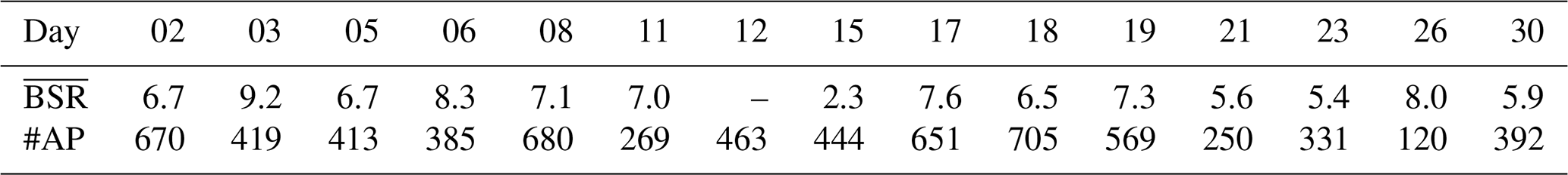
In August 2016, 15 balloons were launched in Nainital, Uttarakhand, India (29.35∘ N, 79.46∘ E; 1820 m above sea level) (Brunamonti et al., 2018). The balloons carried the Compact Optical Backscatter Aerosol Detector (COBALD), which is a lightweight backscatter sonde (Brabec et al., 2012). It measures the backscatter at 940 nm (infrared) and 455 nm (blue visible) in proximity to the balloon. For the detection of the ATAL the short wavelength channel (455 nm) is used (for details, see Hanumanthu et al., 2020). Furthermore, the balloon carried a radiosonde that logged local temperature and pressure. The backscatter signal can be expressed as the backscatter ratio (BSR). The BSR is the ratio between the total backscatter due to aerosols and air molecules and the backscatter due to air molecules alone. Based on calculations of Bucholtz (1995), the BSR has been inferred from the temperature and pressure of the radiosonde and the backscatter of COBALD. Furthermore, a colour index (CI), i.e. the ratio between the 940 and 455 nm aerosol backscatter has been calculated because it allows us to discriminate between large aerosol particles and smaller ones and accordingly between layers of cirrus clouds and ice-free layers of the ATAL. This analysis provided vertical profiles of the aerosol layer for 15 d in August 2016. Table 1 gives a short overview over the measurements. While the BSR is determined for every measurement point during the ascent, here we use the daily, vertical average of the BSR for each balloon flight. Hence, we analyse the day-to-day changes in the measured BSR profiles and do not analyse the BSR for every measurement time step individually. For further details, see Hanumanthu et al. (2020).
Table 1Overview on COBALD measurements in August 2016. is the daily, vertically averaged BSR. The number of measurements, i.e. the number of initialised air parcels per flight, is labelled #AP.
2.2 Lagrangian transport models
Lagrangian backward trajectories are started at the COBALD observations of the ATAL to identify the location and time when air parcels contributing to the ATAL were released at the MBL. For the backward trajectory calculations, two different Lagrangian models were used: the Chemical Lagrangian Transport Model of the Stratosphere (CLaMS) and the Massive-Parallel Trajectory Calculations (MPTRAC) model.
CLaMS is a full chemical Lagrangian transport model that includes modules for irreversible mixing, chemistry and advection (McKenna et al., 2002b, a). Here, we focus on the advection module alone, which applies a fourth-order Runge–Kutta scheme for the trajectory calculations with a default integration time step of 1800 s. The CLaMS model can be used in hybrid vertical coordinates (Mahowald et al., 2002; Ploeger et al., 2010; Pommrich et al., 2014; Ploeger et al., 2021). Near the surface, the hybrid coordinate ζ is an orography-following sigma coordinate and transforms continuously into potential temperature at higher altitudes above around 300 hPa (or 380 K). The vertical velocity can be calculated by the reanalysis diabatic heating rates (diabatic vertical velocity) or by the reanalysis vertical velocities from mass balance (kinematic vertical velocity). CLaMS can be used with both vertical velocity approaches (e.g. Ploeger et al., 2010; Li et al., 2020); however, in most CLaMS studies the diabatic approach is used.
MPTRAC (Hoffmann et al., 2016, 2022) is a Lagrangian transport model for the free troposphere and the stratosphere. It includes modules for advection, diffusion and convection, which are applied in this study. The advection module uses the mid-point scheme for integration with a default time step of 180 s (Rößler et al., 2018). MPTRAC has been further developed for this study to use either pressure or ζ coordinates (kinematic or diabatic vertical velocities) to calculate the trajectories following the approach in CLaMS. In contrast to CLaMS, mixing is computed with two modules that parameterise diffusion and subgrid-scale winds, using given diffusivity coefficients and parameterised subgrid-scale wind fluctuation (Stohl et al., 2005).
Atmospheric models that are used to create reanalysis data need to apply convective parameterisation because they are not able to resolve the small-scale convection processes (e.g. Dee et al., 2011; Hersbach et al., 2020). However, since the reanalysis product only contains the averaged velocities, Lagrangian transport models have to employ a convective parameterisation as well, to simulate unresolved convection. Therefore, the extreme convection parameterisation (ECP) has been implemented recently into the MPTRAC to represent the effects of unresolved convection in the reanalysis data (Hoffmann et al., 2023b). The ECP was first introduced by Gerbig et al. (2003) to estimate the upper limit of convective cloud transport and was later also implemented in HYSPLIT (Loughner et al., 2021). The ECP vertically mixes the air parcels within a convective column by a randomised density-weighted distribution between the surface and the equilibrium level (EL). Hence, it is assumed that the vertical column is well-mixed after a convective event, so that further mixing could not change the distribution anymore.
The stability is assessed with the convective available potential energy (CAPE). CAPE is the integrated amount of work that the upward buoyancy force would perform on a given mass of air if it rose vertically through the atmosphere. If a specific CAPE value is exceeded, which is defined by the user, the convection parameterisation is triggered. The parameterisation scheme is configured for the largest possible enhancement of convective transport, additionally to the already resolved convection in the reanalysis. The CAPE threshold for the triggering of the parameterisation was set to 0 J kg−1 for that purpose. The combination of vertical well-mixing and the most sensitive configuration of the trigger parameter allows an estimation of the upper limit for the convective transport that can be simulated within the given model framework.
Here, in addition, we use the convective inhibition (CIN) as a trigger parameter. The CIN is the energy that air parcels need to overcome when a stable layer below the level of free convection exists. Therefore, if the CIN is larger than a certain threshold, the parameterisation is not triggered anymore. We applied a CIN threshold of 50 J kg−1. This was motivated by spurious convection over the Persian Gulf. Further details are discussed in Sect. 3.2 and Appendix F1.
2.3 Reanalysis data
We used full-resolution ERA5, low-resolution ERA5 and ERA-Interim reanalysis data to drive the backward trajectory calculations with CLaMS and MPTRAC. Both reanalyses have been developed by the ECMWF. ERA-Interim is the precursor of ERA5. The ERA-Interim reanalysis offers 6-hourly meteorological data at around 80 km horizontal resolution on 60 levels. It reaches from the surface up to 0.1 hPa. The ERA-Interim reanalysis is available for the years from 1979 to 2019. The assimilation system for ERA-Interim uses a four-dimensional variational analysis (4D-Var) with a 12 h time window and the ECMWF's Integrated Forecast System (IFS) cycle 31r2 as released in 2006.
The ERA5 reanalysis offers hourly meteorological data on a 30 km horizontal grid (0.3∘ × 0.3∘) over 137 levels from the surface up to 80 km. The ERA5 reanalysis was processed with an improved model version compared to ERA-Interim (IFS cycle 41r2 with 4D-Var assimilation), including novel parameterisations of atmospheric waves and convection. The ERA5 reanalysis covers the time period between 1950 and the present. The increase in spatial and temporal resolution in ERA5 particularly improves the representation of tropical cyclones and convection in the reanalysis in comparison to ERA-Interim and other reanalysis data (e.g. Taszarek et al., 2020; Li et al., 2020). ERA5 was also found to significantly improve Lagrangian transport simulations in the free troposphere and stratosphere (Hoffmann et al., 2019).
The low-resolution ERA5 data set (referred to as ERA5lr) was created by down-sampling of the full-resolution data to a 1∘ × 1∘ horizontal grid and 6 h time steps, applying a truncation to T213 as is specified in the ECMWF Meteorological Archival and Retrieval System. The vertical levels of ERA5 were kept unchanged. Low-resolution ERA5 data were used in previous studies to benefit from the improvements in the ERA5 reanalysis but to avoid high computational costs and costs for handling the much larger number of data compared to ERA-Interim (e.g. Ploeger et al., 2021).
2.4 Simulation scenarios
For the Lagrangian backward trajectory calculations with CLaMS and MPTRAC, the air parcels are initialised at positions of the measured ATAL in August 2016 on 15 measurement days. For every measurement time of the COBALD instrument, i.e. every second, one air parcel is initiated. During a flight the balloons' horizontal drift is below 10 km in the ATAL. The differences are below 50 km in the ATAL when different balloons, from different days, are compared, and hence, they are also negligible. Table 1 shows an overview over the measurements and the number of air parcels initialised per day. Two balloon flights are discussed separately: the flight on 12 August, when a large cirrus cloud covered the full UTLS in the sampled region, and on 15 August, when no ATAL was detected (for details, see Hanumanthu et al., 2020). All air parcels are calculated backward for 90 d to cover the entire Asian monsoon period (JJA).
Table 2Overview of scenarios of 90 d backward calculations performed for the ATAL measurements above Nainital in August 2016. The abbreviation for each scenario contains the reanalysis in the first position, the vertical velocity in the second position and the model in the third position, with each label being separated by a dash. Optional properties are added in the same way in the last position.
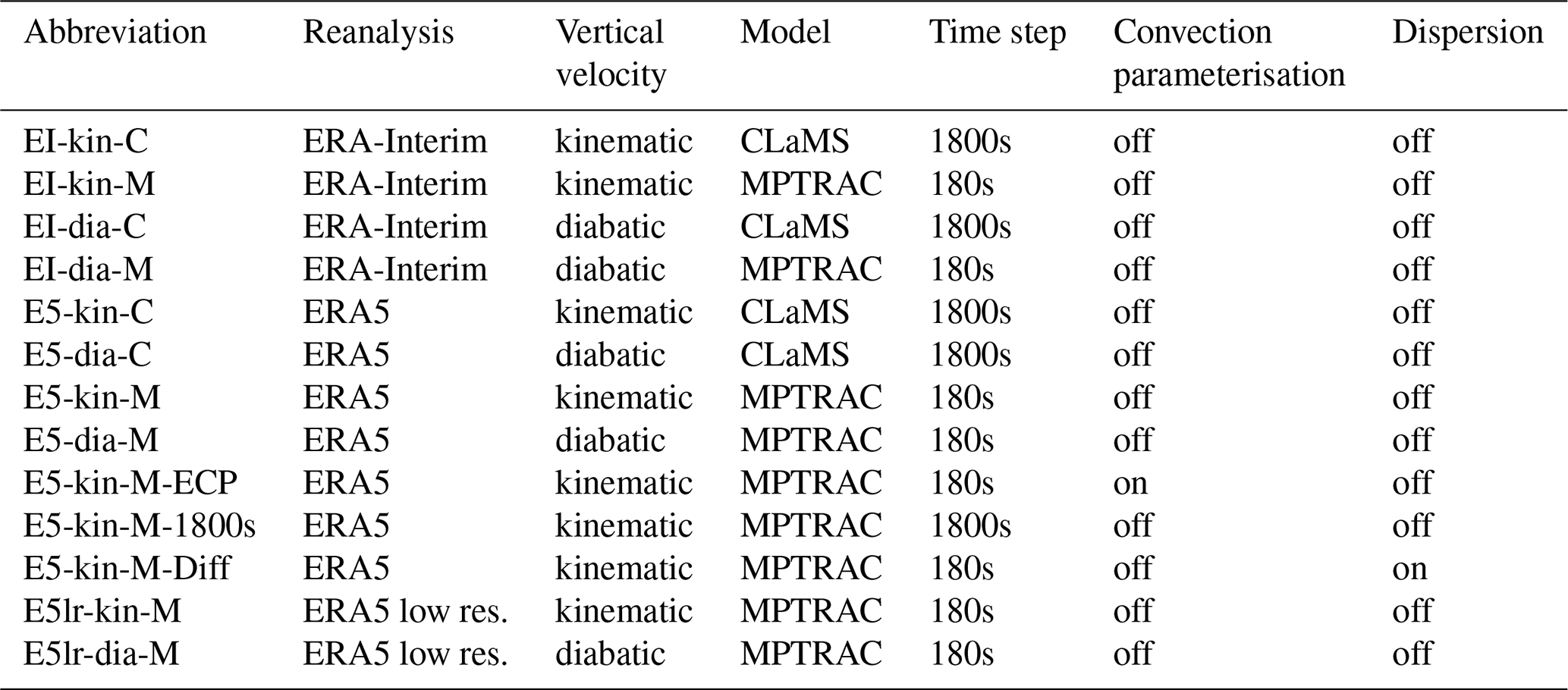
Different scenarios for the calculations have been applied to study the impact of the reanalysis data (ERA5 vs. ERA-Interim), Lagrangian model differences (CLaMS vs. MPTRAC), vertical velocities (diabatic and kinematic) and parameterisations (convection vs. no convection), and the size of the time step (180 s vs. 1800 s) on the simulated transport. We consider the default configurations of the models for the integration time step. Additionally, one scenario with MPTRAC is included, for which instead of initialising one air parcel per measurement point, 1000 air parcels are initialised and random perturbations along the trajectories were added. With this ensemble approach, sampling uncertainties were estimated. For the particle diffusion we used the default settings (see Hoffmann et al., 2022). A summary of all scenarios can be found in Table 2.
2.5 Classification of air parcel origin
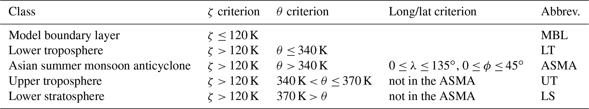
The origin of the air parcels found in the ATAL is classified vertically and horizontally based on the 90 d backward trajectory calculations. Vertically, we follow Hanumanthu et al. (2020) with four classes: the model boundary layer (MBL), the lower troposphere (LT), the upper troposphere (UT) and the lower stratosphere (LS). These vertical layers are defined by values of the vertical coordinate ζ and the potential temperature θ as presented in Table 3. The MBL is defined as the layer below the 120 K ζ level, which approximately corresponds to heights between 2 and 3 km. Accordingly, an air parcel is considered to originate from the MBL if it is located at any time below the 120 K ζ level (Pommrich et al., 2014; Vogel et al., 2019; Hanumanthu et al., 2020).
Table 3Classes for vertical classification of the distributed air parcels. Air parcels have to fulfil all the criteria to be attributed to a specific class. ζ is the vertical hybrid ζ coordinate, θ is the potential temperature, λ is the longitude and ϕ is the latitude of an air parcel.
Hanumanthu et al. (2020) used backward trajectory times between 40 and 80 d. We extended the calculations to 90 d for each air parcel to completely cover the entire Asian summer monsoon season in our analysis. We found that a majority of the transport from the MBL to the ATAL occurred within 90 d (i.e. 60 %–90 % of air parcels reach the MBL during that time), with only a low increase when a longer integration time is used (lower than around 5 percentage points per 10 additional days).
When an air parcel is classified as originating from the MBL, it is also horizontally classified according to the position where it left the MBL for the last time. For this position, we defined several possible source regions. The regions were motivated by different surface characteristics, such as the presence of aerosol or aerosol precursors, and by source regions proposed by earlier studies (e.g. Li et al., 2017; Höpfner et al., 2019; Li et al., 2020; Hanumanthu et al., 2020). For the continents, the following regions are defined: the Asian Highlands, i.e. mostly the Tibetan Plateau and its immediate surroundings (around 60 % of the highlands area); the Indo-Gangetic Plain together with the foothills of the Himalayas; a region south of India plus Sri Lanka; and finally South-East Asia. In particular, for the Asian Highlands we found that 75 % of the air parcels originate from the Tibetan Plateau (heights larger than around 4 km) and up to 98 % originate from the Tibetan Plateau and its immediate surroundings. Other parts of the continents are summarised as the residual continent. For the oceans, three regions were defined: the tropical western Pacific that has been affected by typhoon activity, the Arabian Sea, the Bay of Bengal and the residual oceans. Figure 3a illustrates the different regions. For more detail of the definitions, see Appendix A.
Additionally, for those air parcels that do not originate from the MBL but instead still circulate in the ASMA after 90 d of backward trajectory time, we define the class of the ASMA. For this purpose, we consider a 3D box from 0 to 135∘ E, and from 0 to 45∘ N (magenta box in Fig. 3a) within the UTLS region. Each air parcel within this box is considered to be part of the ASMA.
In the following, we present transport pathways, transport times and possible surface source regions of air mass contributions to the ATAL above Nainital in August 2016. Furthermore, the relation between the observed ATAL's backscatter intensity and different MBL regions is analysed. Our analysis is performed for different simulation scenarios as described in Sect. 2.4.
3.1 Transport pathways from source regions to the measured ATAL
The ASMA extends from north-east Africa to the western Pacific from early June until the end of September; therefore, air parcels circulate in the ASMA over a wide range of longitudes and latitudes. Depending on its extension and position, convection can uplift air from different regions of the Earth's surface – i.e. with different chemical composition – into altitudes of the anticyclone. Within the ASMA, the air from different origins will be mixed, for example due to instabilities of the ASMA (e.g. Gottschaldt et al., 2018). Different source regions can contribute to the chemical composition of the ASMA; therefore, trace gases and aerosol are in general not homogeneously distributed within the ASMA. The ASMA can show a bimodal structure, where one circulation centre is placed roughly over Iran and the other one is centred roughly over South-East Asia and where the separation of the two modes varies in time. The shape of the ASMA varies between normal and bimodal on a daily basis; however, in the climatological mean it is controversially discussed if two modes exist. In addition smaller eddies can be separated to the west and to the east (sometimes referred to as third mode) (Yongfu et al., 2002; Nützel et al., 2016; Honomichl and Pan, 2020; Manney et al., 2021).
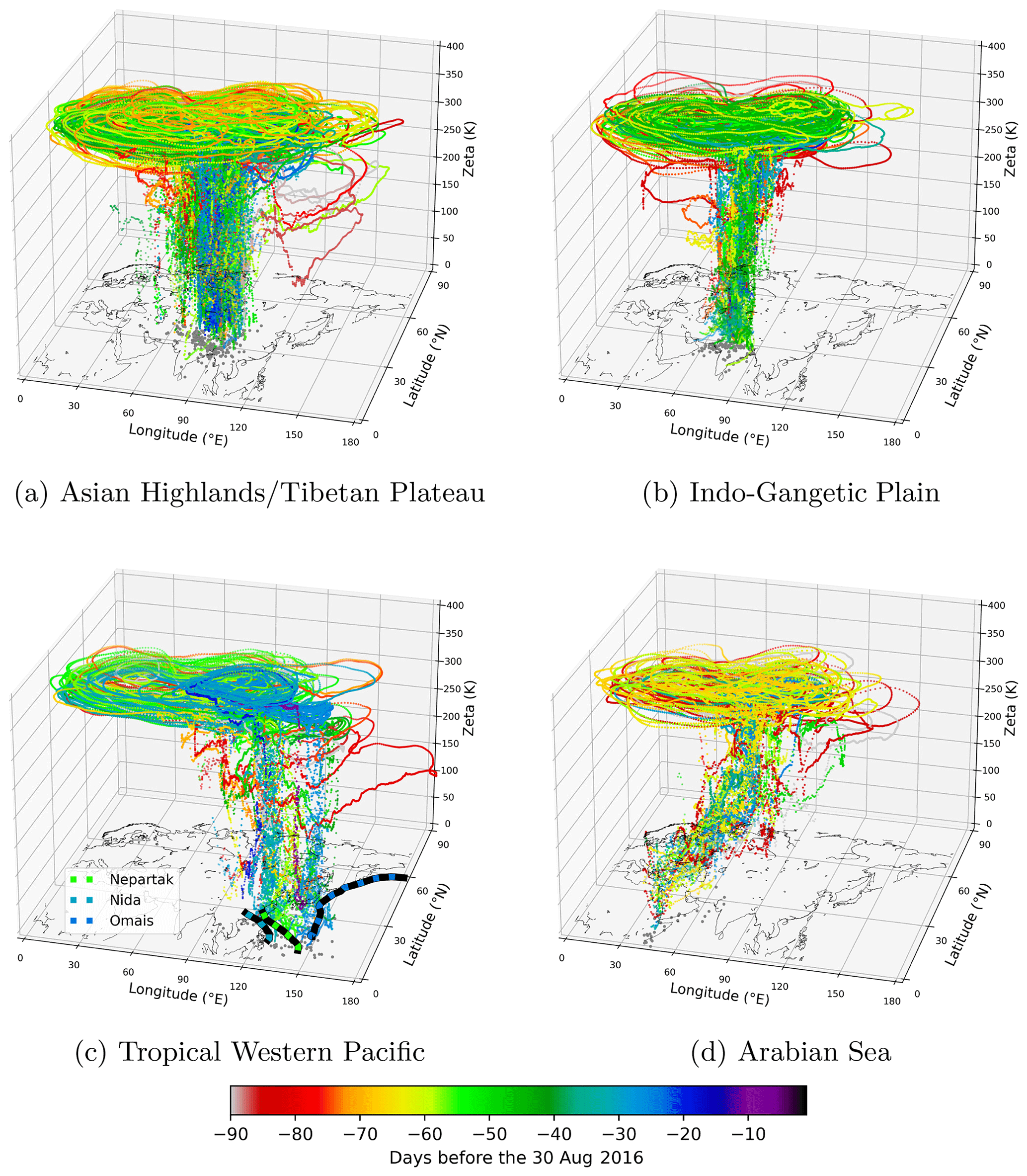
Figure 1Examples of backward trajectories of air parcels of all of the 15 measurement days from the ATAL measurement to the MBL, categorised by the source region. Shown are trajectories of scenario E5-kin-C. Colours indicate the time when the air parcels left the MBL. Grey dots at the bottom show the horizontal position of the air parcels (APs) 48 h before they crossed the MBL from below. In (c), additionally, tracks of three typhoons are plotted (Nepartak, Nida, Omais), where each point is coloured like the trajectories and the mean time of occurrence.
Figure 1 shows four example transport pathways of air parcels from different regions at the MBL to the measured ATAL over Nainital in August 2016 due to convective transport. For the illustration of transport pathways we use the scenario E5-kin-C because it is representative with regard to the general patterns also for the other scenarios, while particular differences are analysed in depth later. We also include trajectories of all days of measurement for the illustration.
Figure 1a shows injections into the centre of the ASMA in proximity to Nainital, originating from the Tibetan Plateau. Throughout the season the air is pumped upward into the ASMA on timescales of hours to a few days (50 % of transport from the MBL of Asian Highlands into the UTLS is within less than half a day; see also Tables E2 and E1). In the ASMA, air masses are uplifted by diabatic heating superimposed by the anticyclonic flow until they meet the measurement points over Nainital. Air parcels circle in a rising spiral, within the two modes of the ASMA, until they meet the measurement points over Nainital (e.g. Vogel et al., 2019). A small number of air parcels leaves the ASMA for a while and is subsequently transported along the subtropical jet, circumnavigating the Earth, until the air parcels are trapped in the ASMA again. Thereafter, the air parcels also arrive at the measurement points.
Figure 1b shows the uplift of air into the ASMA mostly over the Indo-Gangetic Plain and in the foothills of the Himalayas. The air masses were transported mainly directly from the Indo-Gangetic Plain into the UTLS. The transport in the ASMA and sporadically along the jet streams is the same as for the Tibetan Plateau. Hence, in the foothills of the Himalayas, transport pathways from two regions with two very different land-cover properties converge: the Tibetan Plateau and the Indo-Gangetic Plain. The transported air masses subsequently mix in the ASMA.
Figure 1c illustrates transport from the Pacific to the measurement locations in relation to three typhoons (named Nepartak, Nida and Omais) that occurred during the relevant time period (we use the typhoon best-track data of the Japan Meteorological Agency). The typhoons uplift a large number of air parcels from the maritime surface into the eastern edge of the ASMA. Depending on the position of the ASMA modes and the typhoons, the uplifted air masses circulate on the outer edge of the ASMA (e.g. for Nida and Nepartak) or they circle mostly in the eastern mode and the inner area of the ASMA (e.g. Omais). Because of the multiple circulations in the ASMA the typhoons influence the measurements with a delay in time of several days. The impact of typhoons on the air masses in the ASMA and the ATAL has been reported before (e.g. Li et al., 2020; Hanumanthu et al., 2020).
Figure 1d presents a transport pathway from the Arabian Sea to the ASMA. The transport of the air parcels occurs in four steps. At first, the air leaves the MBL for the free troposphere over the Arabian Sea, possibly due to shallow, maritime convection. Secondly the air is transported eastward within the free troposphere to the foothills of the Himalaya or to the Bay of Bengal. During this transport, over the Indo-Gangetic Plain or the Bay of Bengal, deep convection uplifts the air to the southern edge of the ASMA, which is the third step of transport. In the last step, the air masses circle in the ASMA until they are measured at Nainital. A similar long-range transport pathway to the Himalayas can be observed for the Bay of Bengal. However from the Bay of Bengal more air parcels can enter the ASMA directly from the maritime boundary than from the Arabian Sea. This is likely related to the overall Asian monsoon circulation, in which air masses are transported in the troposphere from the Arabian Sea (AS) across India, while the Bay of Bengal is a known source of deep convection. Moreover, those air masses that are convectively uplifted into the UTLS over the AS, are often located at the outer edge of the anticyclone and westward from Nainital. Hence, this transport pathway to Nainital is much less probable. In Appendix B, the transport pathways from the Bay of Bengal, south India, South-East Asia, and the remaining ocean and continent are presented as well.
3.2 Scenario intercomparison of contributions from source regions and related transport pathways
Although the general transport pathways from the MBL to the measurement locations, as presented in Sect. 3.1, exist in all simulation scenarios with the Lagrangian transport models, the contributions of different source regions can differ, depending on the scenario used. Here, we present the differences and similarities of the vertical and horizontal distribution of the source regions between the different scenarios. For the analysis, we use all 15 measurement days and 90 d backward trajectories.
First, the fraction of air from different atmospheric layers is calculated for all model scenarios (see Fig. 2). Wide agreement can be found with ERA5 even when models, integration step sizes and vertical velocities are varied (except when the extreme convection parameterisation is employed). The total amount of transport from the MBL lies between 74 % and 80 % for the ERA5 scenarios. The distribution from the LT, UT or LS shows only some minor differences. Large disagreement is found between the diabatic and kinematic vertical velocities using ERA-Interim. With kinematic vertical velocities, only around 60 % of the air parcels originate in the MBL, while with diabatic velocities the results are closer to the ERA5 scenarios (around 75 % amount of transport from the MBL). Disagreement in ERA-Interim, when varying the vertical velocities, was also found in other studies (e.g. Ploeger et al., 2010; Li et al., 2020; Legras and Bucci, 2020). The low-resolution ERA5 data set maintains the higher consistency of ERA5 in comparison to ERA-Interim and the total transport from the MBL is only slightly reduced, probably because the vertical resolution is unchanged and higher vertical velocities over the continent also remain higher in ERA5lr as well. A large increase in transport from the MBL is caused by the onset of the convection parameterisation in scenario E5-kin-M-ECP. In this case only around 10 % of the air parcels originate outside the MBL and no air parcels originate in the LT. The latter can be explained, when following the air parcels backward in time: if the air parcels enter the LT during backward calculations they likely enter a region where the ECP is triggered. Then transport into the MBL takes place immediately.
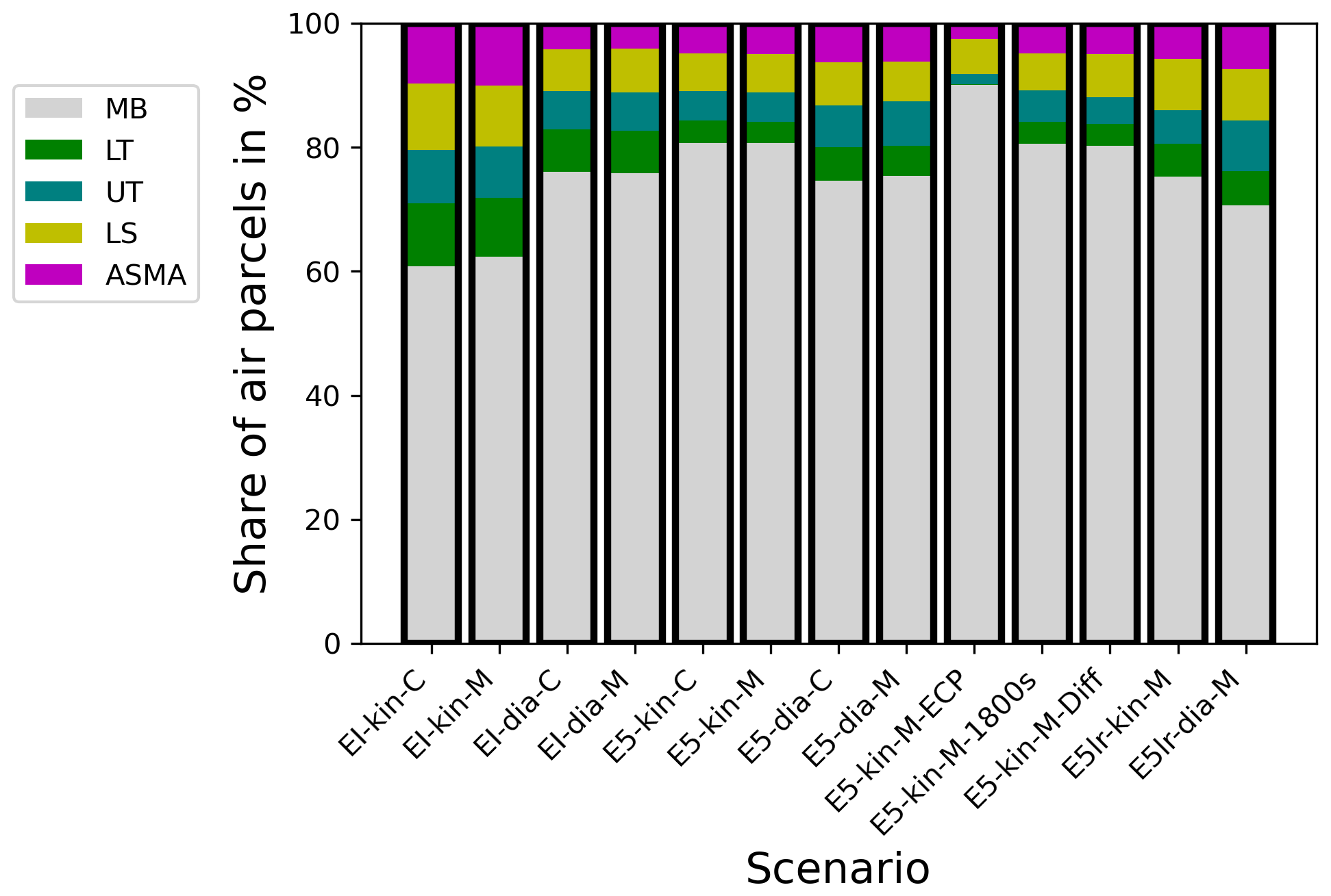
Figure 2Vertical classification of air parcel origin after 90 d of backward trajectory calculations with different scenarios.
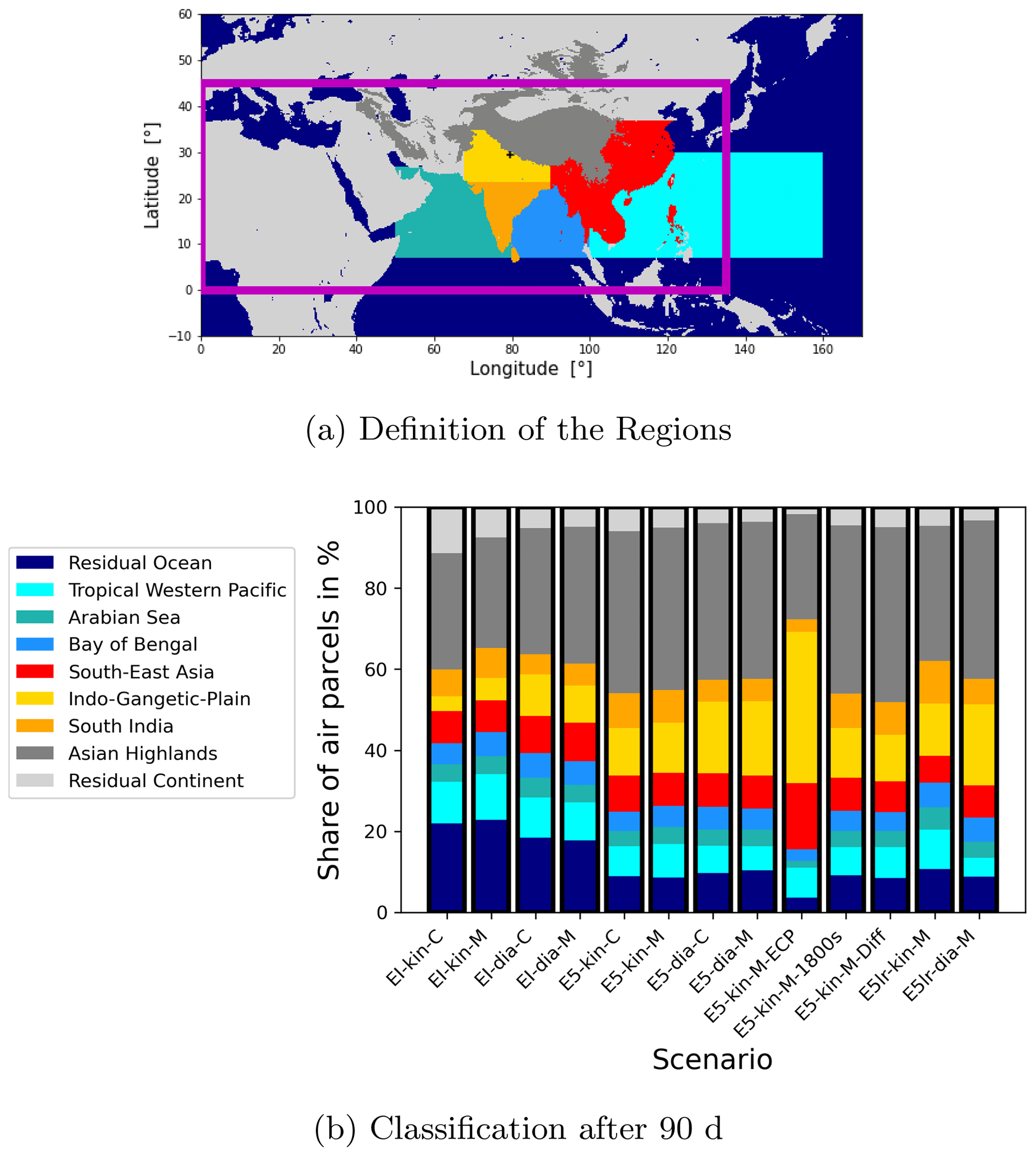
Figure 3Panel (a) shows the definition of contributing regions. The purple box marks an area that contains most of the air parcels that circulate in the ASMA. Panel (b) shows the horizontal classification of the air parcels according to the surface regions after a 90 d backward trajectory time. Shown is the fraction of air parcels that reach the MBL.
Second, the fraction of air from different MBL regions contributing to the ATAL is compared for all model scenarios (see Fig. 3b). Model scenarios driven with ERA5 show very similar results. For ERA5 scenarios, about 40 % of the air parcels that originate from the MBL originate from the Tibetan Plateau and other Asian Highlands. Around 5 % to 10 % of air parcels each come from south India and South-East Asia. The contributions from the Indo-Gangetic Plain is between 10 % and 20 %, with higher values for diabatic calculations. The Indian subcontinent, i.e. the Indo-Gangetic Plain and south India together have the largest contribution from the continent. Around 25 % of the air parcels that come from the MBL originate from oceans, mostly the western Pacific and many are related to tropical cyclones. In contrast to ERA5, using ERA-Interim increases the contribution of air parcels from the oceans by up to around 40 %. This increase does not rely on the variation in the vertical velocity and is robust for all scenarios driven with ERA-Interim. The contribution from the Indo-Gangetic Plain is reduced to 5 %–10 % with ERA-Interim compared to ERA5 and also shows a difference between diabatic and kinematic velocities. With the extreme convection scenario the contribution from the oceans is smaller than in the cases with ERA5. However, with the ECP the contribution from the Indo-Gangetic Plain and the foothills of the Himalayas increases strongly at the expense of contributions from the Tibetan Plateau and the oceans. As a consequence of the persistent occurrence of CAPE above South Asia in summer, the scenario with ECP simulates more and deeper convective updrafts in this region than the scenarios without ECP. Hence, transport from the MBL that would be missed without the ECP, increases the contributions from South Asia. Finally, the ERA5 low-resolution scenarios show a decrease in consistency between the diabatic and kinematic approach. The kinematic approach has a bias to more transport from the ocean in the low-resolution data in comparison to the fully resolved ERA5 data, while the results for the diabatic approach show only a minor difference to the fully resolved ERA5 data in the statistics.
With the ensemble scenario (E5-kin-M-Diff), we tested uncertainties due to unresolved sub-grid-scale wind fluctuations and found standard deviations lower than 1 % for the distribution of air parcels to different vertical layers or horizontal regions. Therefore, the sub-grid-scale wind fluctuations do not cause a serious bias in this analysis. The ensemble scenario E5-kin-M-1800s was used to investigate possible biases between the models due to different time steps. However, as the results remain almost unaltered for MPTRAC when the time step is varied from 180 to 1800 s, we rule out a serious bias for our analysis.
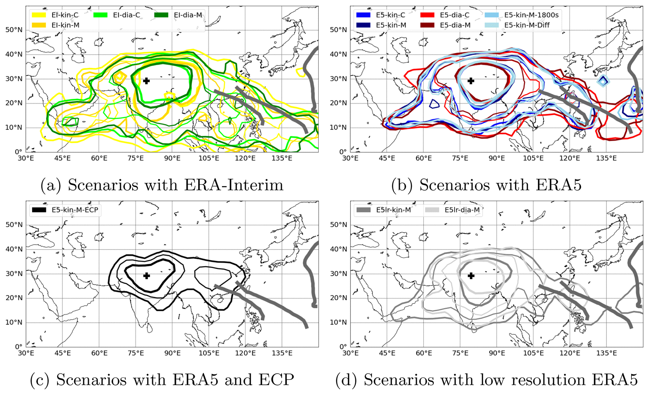
Figure 4Contours of the probability density function (PDF) of the surface sources for 90 d backward trajectories and all measurements. Colours indicate the different scenarios. For each scenario the inner, thick contour encloses 50 % of the points where air parcels left the MBL and the outer contour encloses 90 % of them. In between, a thin contour is shown for 75 %. For the sake of clarity, the contours are smoothed by a Gaussian kernel. The black cross indicates the position of Nainital. The three thick grey lines show typhoon tracks.
The probability density function (PDF) for air parcels leaving the MBL is shown in Fig. 4. All scenarios except the ECP scenario show a very similar pattern, with most dominant transport from a region centred at the eastern foothills of the Himalayas and the south-eastern Tibetan Plateau (around 50 %), while transport from other regions is much less but not irrelevant. If contours for ERA5 scenarios and ERA-Interim scenarios are compared, air parcels are dispersed more with ERA-Interim, particularly in the direction of the ocean, while ERA5 resolves more transport at the continent and disperses the air parcels less. Using the scenario with ECP deforms the pattern even more because more transport happens then at the Indo-Gangetic Plain, due to higher convective available potential energy (CAPE) in this region than on the Tibetan Plateau. The results of the ECP depend on the selection of the CIN and CAPE thresholds. We used the CIN threshold to remove spurious parameterised convection over the Persian Gulf (see Appendix F).
In summary, ERA5 provides improved robustness against changes in the vertical velocity between the kinematic and diabatic approach in comparison to ERA-Interim and yields very good agreement between the two Lagrangian models. Using the ECP in MPTRAC indicates that even scenarios with ERA5 could miss the effects of unresolved convection, particularly locally over the Indo-Gangetic Plain. This leads to difficulties when distinguishing the contributions from the Tibetan Plateau and the Indo-Gangetic Plain. When air parcels pass the region around the Himalayas during the backward trajectory calculations, the position where they are transported back into the MBL is sensitive to the representation of the convection. With the ECP, convection is enhanced over the Indo-Gangetic Plain (IGP). Hence, far more air masses are attributed to the IGP with the ECP, while without the ECP most air parcels originate from the Tibetan Plateau (TP). Further improvement in reanalysis and parameterisation are needed to remove this uncertainty.
3.3 Scenario intercomparison of the temporal evolution of transport from the MBL to the measured ATAL
The transport time of the air parcels from the MBL to the ATAL affects aerosol formation. The time of the transport is therefore an important parameter to analyse. An analysis of the temporal evolution of the transport process from the MBL to the measurements also highlights some differences between the model scenarios.
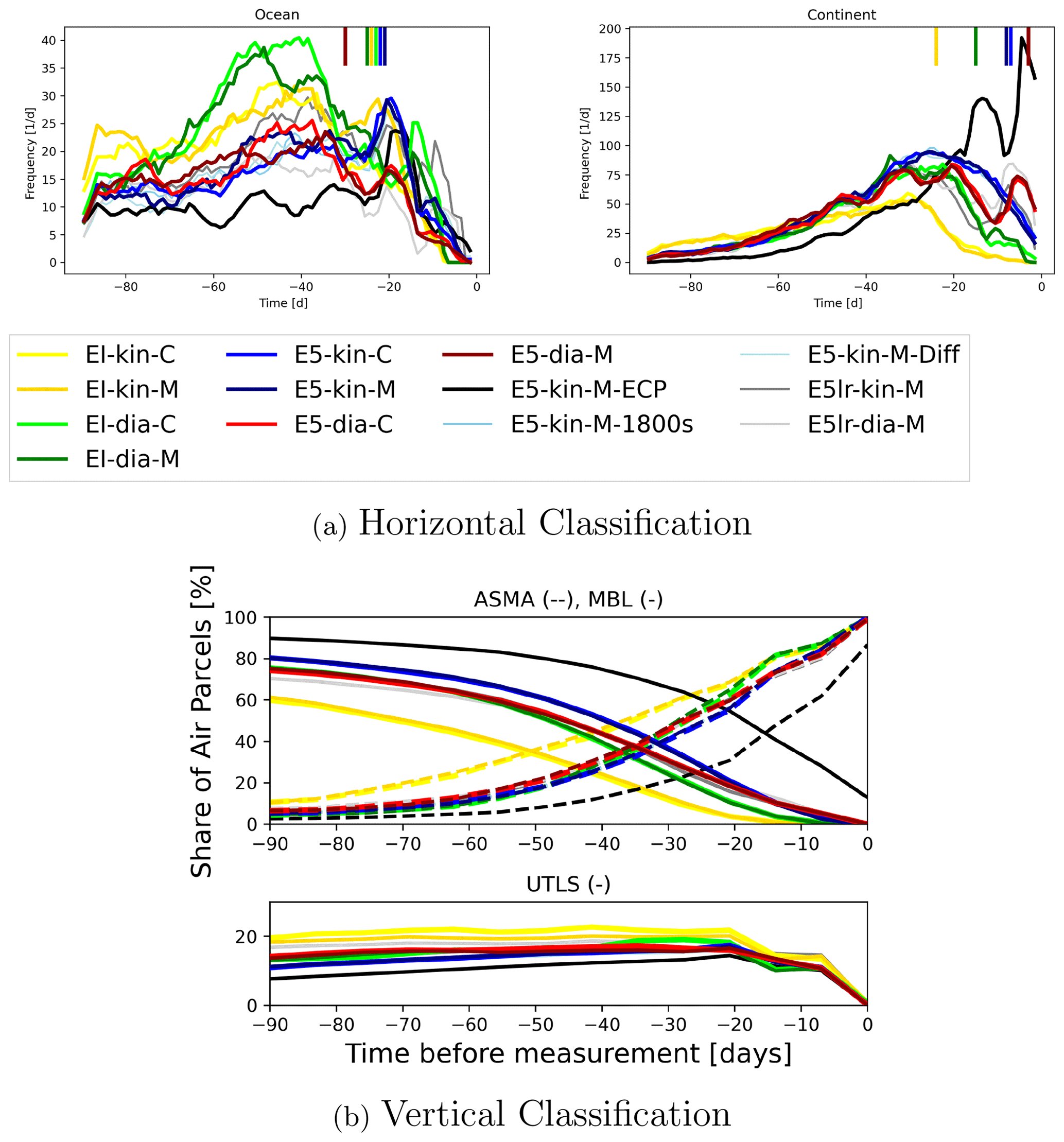
Figure 5Time evolution of transport from the MBL to the ASMA within 90 d, relative to the start of the trajectories. Panel (a) shows the frequency of air parcels leaving the MBL smoothed with a 1-week running mean. The short lines at the top indicate for some scenarios the maximum time for the first 300 air parcels with the smallest transport time. Panel (b) shows the share of air parcels that are within the ASMA (upper panel, dashed line), the share of air parcels that are in the MBL (upper panel, solid line) and the share of air parcels that are in the UTLS (lower panel, solid line).
To emphasise the possible lifetimes of air masses transported to the location of the measurements in the UTLS, Fig. 5a shows the frequency of air parcels leaving the MBL per day at different times before the measurements for the different scenarios. These frequencies are classified as belonging to two categories: the continents and the oceans. Most of the relevant maritime convection (e.g. typhoons) that transport air masses out of the MBL into the upper atmosphere take place more than 2 weeks before the measurements. This can be found for all scenarios. For scenarios with ERA-Interim the frequency of air parcels leaving the MBL is higher than for ERA5 if transport times longer than 40 d are considered, in particular for the diabatic scenarios with ERA-Interim.
For ERA-Interim only a few air parcels originate from the continent with transport times of less than 2 weeks, independent of the vertical velocity used (diabatic or kinematic). This resembles the results of Hanumanthu et al. (2020), who used diabatic CLaMS trajectories driven by ERA-Interim. In contrast, all scenarios with ERA5 show that air from the continent can be transported much faster to the location of the measurements even in much less than 2 weeks. This is likely due to a better representation of convection in ERA5 in comparison to ERA-Interim. This fast transport at the beginning is maintained with the low-resolution ERA5 data, although it is reduced in temporal and spatial resolution in comparison to the full ERA5. Furthermore, using the ECP reveals that ERA5 also potentially underestimates convection in the first days. The fast transport with ECP is caused by the frequent triggering of the parameterisation over the continent, particularly over the Indo-Gangetic Plain, where the atmosphere often shows convective parameters (CAPE, CIN) that suggest unstable conditions. However, our approach of the ECP has to be regarded as the upper limit for the convective transport that can be simulated within the given model framework. In summary, in ERA5 air masses are transported from the continental MBL to the ATAL relatively fast (within 2 weeks), so that fewer air parcels remain to originate from the maritime MBL, while with ERA-Interim this effect reverses. With ERA-Interim only few air parcels are transported fast to the ATAL from the continent, while more and older air parcels originate from the oceans.
Figure 5b shows the accumulation of air parcels within the ASMA during the transport processes to the ATAL over Nainital. The differences between the scenarios can be understood when the transport is described following the calculations backward in time, i.e. when we look at the “draining” of the ASMA during backward calculations. Our calculations show that in all scenarios most of the air parcels start in the ASMA. When the air parcels are traced back in time, the share of air parcels in the ASMA for scenarios with ERA5 and ERA-Interim starts to diverge. In the first 2 weeks backward in time (−14 to 0 d), scenarios with ERA5 show more transport back into the MBL than scenarios with ERA-Interim; i.e. the share of air parcels in the MBL increases faster with ERA5 and the share in the ASMA declines faster than with ERA-Interim. This is in agreement with faster transport from the continent with ERA5 than with ERA-Interim as described before. After calculating the trajectories further back in time (longer than 2 weeks), the share of air parcels in the ASMA starts to converge again for the ERA-Interim scenarios with diabatic velocities (EI-dia-C, EI-dia-M) and the ERA5 scenarios. This convergence is partly caused by the increased backward transport to the maritime MBL in the scenarios with ERA-Interim and the diabatic scheme, while with ERA5 the transport to the maritime MBL is smaller in comparison (see also Fig. 5a, left panel, −70 to −30 d). The ERA-Interim scenarios with a kinematic approach (EI-kin-C, EI-kin-M) diverge further from all other scenarios, showing a much lower share of air parcels in the MBL than other scenarios and the most air parcels in the UTLS. After around 2 weeks the share of air parcels in the UTLS increases more in the scenarios with ERA-Interim and kinematic vertical velocities (see lower plot in Fig. 5b) than in all other scenarios. Ploeger et al. (2010, 2011) demonstrated more dispersion in backward trajectory calculations with ERA-Interim and the kinematic approach than with the diabatic approach. This effect explains the large difference between the scenarios EI-kin-C and EI-kin-M from the other scenarios and why many air parcels are transported back into the UTLS with these scenarios.
3.4 Backscatter changes associated with changes in the transport and source regions
Hanumanthu et al. (2020) found a distinct day-to-day variability in the ATAL backscatter intensity. This variability may be correlated with daily to weekly changes in the transport within the highly variable anticyclone and variability in tropical convection and therefore with changing surface source regions. To analyse the changes from measurement to measurement, the contribution of different source regions to the vertical ATAL profile has been reconstructed for every balloon flight separately. Subsequently, the relative deviation of the contribution of a specific region on 1 d from the mean contribution during all measurements normalised by the mean contribution was calculated as a relative, normalised deviation (in percent). Accordingly,
was calculated for every day of a selected scenario. RND(t) denotes the relative, normalised deviation for measurement day t, and C(t) denotes the contribution of air parcels for the measurement day t from the selected region. The contribution C(t) is measured as the ratio between the number of air parcels from the selected region to the total number of air parcels for the measurement day. is the time-averaged contribution over all measurement days for the selected scenario. This calculation has been done for all scenarios separately to allow a direct day-to-day intercomparison of the scenarios.
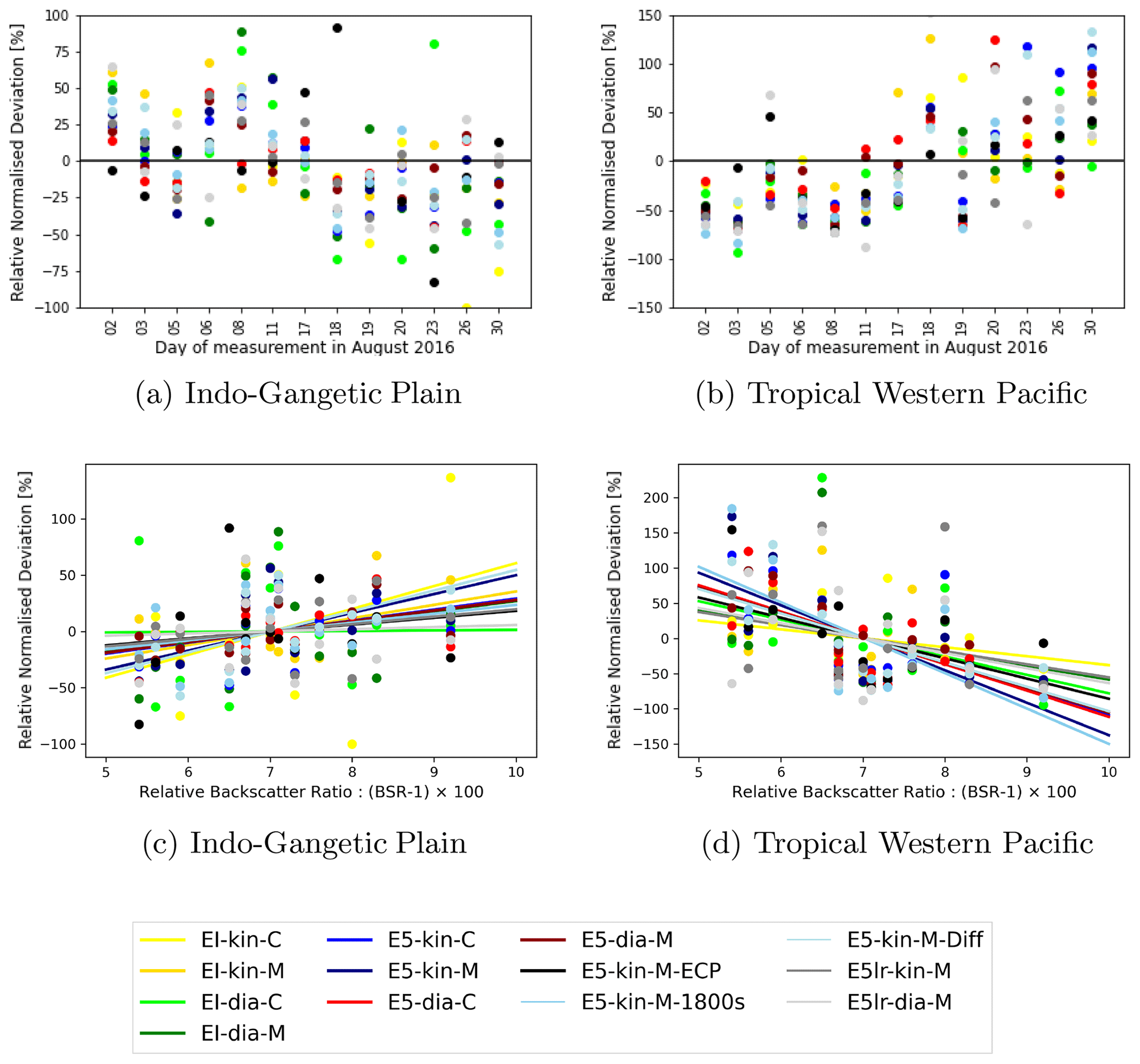
Figure 6Panels (a) and (b) show the relative, normalised deviation for each measurement day of the Indo-Gangetic Plain and the tropical western Pacific. Panels (c) and (d) show the relations between the daily averaged backscatter intensity and the relative, normalised deviation. The lines show linear fits for each scenario. Coloured dots show results for all scenarios. The colour code for the dots is the same as in Fig. 5, where every colour corresponds to one scenario.
Figure 6 shows the normalised deviations for the Indo-Gangetic Plain and the western Pacific Ocean for 13 measurement days. The days with no ATAL or with large cirrus cloud coverage have been excluded from the analysis (12 and 15 August). Furthermore, we focus on the Indo-Gangetic Plain and the western Pacific Ocean as they show the most robust and significant results in comparison to other source regions.
Figure 6a and b show the relative, normalised deviation for every measurement day. Overall, all scenarios indicate a clear temporal evolution of the contribution from the two regions during the weeks of the campaign in August: the scenarios show that in the early phase of the campaign (2, 3, 6 and 8 August) the contributions from the Indo-Gangetic Plain were enhanced relative to other days, while in the later phase (19–30 August) contributions from the Indo-Gangetic Plain were relatively low. For contributions from the western Pacific the opposite is found because of the increased impact of typhoons on the measurements at the end of August (see Fig. 6a, b). From day to day, the relative normalised deviation changes in absolute terms with the order of magnitude of 10 % (i.e. 10 %–100 %), while the total change in the relative normalised deviation during the period is roughly 90 %. For some measurement days, the scenarios show similar day-to-day differences (e.g. 2–8 August for the tropical western Pacific), but for other periods the day-to-day variability differs strongly between scenarios (e.g. 23–30 August for the tropical western Pacific).
Figure 6c and d show the relation between the averaged measured BSR for every day and the daily relative, normalised deviation. For the Indo-Gangetic Plain in all scenarios large backscatter ratios coincide with large normalised deviations, although in some scenarios this relation is considerably weak. For the tropical western Pacific, in all scenarios low backscatter ratios clearly coincide with higher normalised deviations.
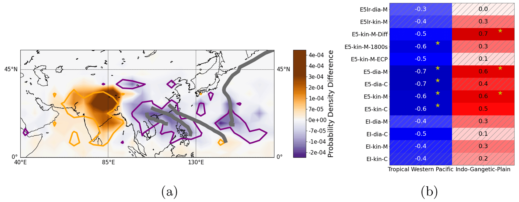
Figure 7(a) Difference between the source region PDF of the 5 d with maximum ATAL backscatter intensity and 5 d with minimum backscatter intensity, derived from the multi-scenario mean. The orange contours show areas where at least two-thirds of the scenarios indicate high values during a strong ATAL. The purple contours show the same for the weak ATAL cases. Data are given on a 5∘ grid. The grey lines indicate the tracks of tropical storms that influenced the measurements. (b) Spearman correlation coefficient for the relation between the daily BSR and the contributions of different regions for different scenarios. Hatched areas indicate insignificant results (p value higher 0.10). Boxes with yellow stars indicate p values lower than 0.05. Colours emphasise positive (red) and negative (blue) correlations.
To further compare transport on those days with a low ATAL backscatter intensity above Nainital to that on those days with a high one, we also calculated the probability density functions (PDFs) of surface source regions for each day separately. In particular, we selected the 5 d with strongest (3, 6, 26, 17, 19 August) and the 5 d with the weakest backscatter intensity (21, 23, 30, 18, 5 August) for the analysis. Figure 7a shows the differences between the two PDFs for the multi-scenario mean. The results indicate that transport from the Indo-Gangetic Plain, India; the Bay of Bengal; and the northern part of the Tibetan Plateau may have strengthened the ATALs backscatter intensity during the measurements. The intensity of the ATAL over Nainital again seems to be low when more transport from the tropical cyclones and the region of their landfall occurred. Although the PDF differences vary strongly from scenario to scenario (see Fig. D1 in the Appendix), at least two-thirds of the scenarios agree on these characteristics.
For a complete analysis, we used the Spearman rank-order correlation coefficients to check whether there is a monotonic relation between the measured backscatter and the contribution of specific regions. Figure 7b summarises these correlations for the Indo-Gangetic Plain and the area of active typhoons at the tropical western Pacific. Correlations to other regions can be found in the Appendix in Fig. E1.
We find a significant (p < 0.1) and robust negative correlation between the backscatter intensity of the ATAL and the western Pacific influenced by typhoons. This correlation remains to be present both for the simulation with ECP with maximum strength of convection and with ERA-Interim where in contrast convection is underestimated. Most scenarios also indicate a positive correlation between the backscatter intensity of the ATAL and enhanced contributions from the Indo-Gangetic Plain. Although, impacts of unresolved convection can likely be neglected for the relation to the western Pacific, the correlation for the Indo-Gangetic Plain changes substantially from 0.6 to 0.1 with parameterised convection (see E5-kin-M-ECP). Moreover, for the Indo-Gangetic Plain the correlation in the scenarios E5lr-dia-M and EI-dia-C remains insignificant. The most significant results however, are obtained in the ERA5 scenarios, supporting the hypothesis that polluted air from the Indo-Gangetic Plain led to higher backscatter intensity and vice versa clean maritime air from the western Pacific lead to a dilution of the ATAL and therefore to a weaker BSR intensity.
Most scenarios furthermore have a positive correlation for contributions from the Arabian Sea, the rest of India and the Bay of Bengal. Such relations seem plausible given the transport pathways from the Arabian Sea and the Bay of Bengal to the ATAL over Nainital, which include a period of horizontal transport in the polluted troposphere over India before a second step of upward transport in deep convection. Additionally, air masses from the Arabian Sea could carry dust from the Arabian Peninsula. Air from South-East Asia is also weakly correlated with a decrease in the ATAL backscatter intensity, which is possibly related to the landfall of some typhoons.
Other source regions have been considered to establish such relations, but given the limited number of data and systematic model uncertainties, no further robust results were found. The positive relation between the Asian Highlands, i.e. mostly the Tibetan Plateau, and the backscatter intensity of the ATAL, found by Hanumanthu et al. (2020) was reproduced for similar scenario set-ups (see EI-dia-C). However, some scenarios even show negative correlations. To check whether our result could depend on the definition of the Asian Highlands, we moreover calculated the correlation with a more narrow definition, focused on the Tibetan Plateau, but we still obtained ambiguous correlations.
Our results corroborate that the transport calculations presented here are capable of capturing the general evolution and patterns during the course of August robustly but might differ if day-to-day changes are considered. The observed general temporal evolution might be related to a large-scale change in the meteorological conditions during August that led to a shift to more air masses from the western Pacific and prior typhoons and less transport from the Indian subcontinent. The differences in the representation of day-to-day changes might arise from the uncertainty about the daily changing convection.
In this study, we investigated the source regions of the ATAL in August 2016. To identify the source regions at the MBL and the transport pathways contributing to the ATAL and to investigate the sensitivity of the applied methods, different trajectory calculations were conducted. Simulations with different model scenarios using different Lagrangian transport models (CLaMS and MPTRAC), wind data (ERA-Interim and ERA5), vertical velocities (kinematic and diabatic), integration time steps and a convection parameterisation (ECP) were analysed. Additionally, we correlated daily contributions of source regions at the surface to daily measured COBALD backscatter intensities at ATAL altitudes to quantify the role of the regions for the intensity of the ATAL.
Most of the air from the MBL that influenced the measurements originated on the Tibetan Plateau (i.e. ≈ 30 %–40 % of air masses originating at the MBL). This is found for all scenarios, except for the scenario with the extreme convection parameterisation. In the scenario with the ECP (E5-kin-M-ECP), the Indo-Gangetic Plain contributes most (≈ 30 %). The Indo-Gangetic Plain is the second-largest continental contributor (10 %–20 %) to the air masses influencing the measurements in all other scenarios (except for ERA-Interim with a diabatic approach). The contribution from the Indo-Gangetic Plain, however, is much smaller than from the Tibetan Plateau in those scenarios. In summary, most of the upward transport takes place at the eastern part of the Indo-Gangetic Plain that extends to the Bay of Bengal, including the foothills of the Himalayas and the Tibetan Plateau. These regions have been found to be dominant for the transport into the ASMA and the ATAL also by other studies (e.g. Bergman et al., 2012; Bucci et al., 2020; Hanumanthu et al., 2020).
In our simulations, a small amount of air was transported from South-East Asia and North India to the ATAL as well. Such transport processes contributing to the ATAL have also been reported before (e.g. Vernier et al., 2018; Bucci et al., 2020; Zhang et al., 2019a, b, 2020). Air masses from the maritime boundary layer were transported to the measurement locations in significant numbers as well. This includes mostly air masses from surrounding seas, such as the Arabian Sea, the Bay of Bengal and the western Pacific. Typhoons in the tropical western Pacific played an important role for the transport process from the maritime boundary layer, which is in good agreement with previous studies, which showed their relevance for the UTLS and the composition of the ATAL (Li et al., 2017, 2020; Hanumanthu et al., 2020).
By studying the transport pathways and times, we showed some systematic differences between simulation scenarios that are related to the representation of convection and the diabatic ascent in the ASMA. ERA5 has a better representation of convective updrafts and tropical cyclones compared to the ERA-Interim reanalysis, attributed to its better spatial and temporal resolution and other improvements in the ECMWF forecast model and data assimilation scheme. Therefore, the fraction of air from the MBL transported upward to ATAL altitudes is lower or about equal in scenarios with ERA-Interim in comparison to scenarios with ERA5. This is in particular true over the continent. Hence, in ERA-Interim, convection over the continent is less frequent than in ERA5, so that larger fractions of air parcels originate from remote maritime regions with ERA-Interim (40 % vs. 23 % of all air parcels from the MBL).
ERA-Interim simulations also show strong differences with regard to the transport from the MBL into the UTLS, when the vertical velocity is varied between diabatic velocities (75 % of all air parcels) and kinematic velocities (60 % of all air parcels). These differences between kinematic and diabatic trajectories are strongly reduced when ERA5 is used, where the diabatic approach shows similar fractions of air transported from the MBL to ATAL altitudes as the kinematic approach (74 % vs. 80 %). Large differences with regard to the vertical transport in typhoons between ERA5 and ERA-Interim have been reported before by Li et al. (2020), and an improvement in consistency between vertical velocities has been reported by Legras and Bucci (2020) in the Asian monsoon region.
Although ERA5 resolves convection better than ERA-Interim (Hoffmann et al., 2019), it might still underestimate the extent of fast vertical transport caused by deep convection in the foothills of the Himalayas and at the Indo-Gangetic Plain. This possible deficiency is indicated by the simulation scenario with ECP, which shows a strong increase in convection near Nainital on the Indo-Gangetic Plain and in the foothills. Our results show that ERA5 provides a significant improvement for the simulation of transport processes in the Asian monsoon region with regard to the consistency between scenarios with different models and vertical velocity schemes. However, ERA5 possibly still has limitations with regard to the representation of the convection, which needs to be evaluated in further studies that take observations of convection into account. In addition, our study shows minor differences for the employed Lagrangian models (MPTRAC and CLaMS). These differences are likely caused by differences in the integration scheme and the interpolation method. Both models are equally valuable in the case of the present analysis.
Taking into account the measured backscatter intensity of the ATAL, we found two regions with a significant and robust impact on the ATAL's variability. Meteorological conditions that are favourable to transport from the Indo-Gangetic Plain increase the ATAL backscatter intensity, while conditions favourable to transport of air masses from the tropical western Pacific and the influence of typhoons decrease the ATAL backscatter intensity. In case of the tropical western Pacific, these findings hold for the different sensitivity calculations carried out, and hence we corroborate the results by Hanumanthu et al. (2020), by showing that this correlation is robust despite the systematic uncertainties represented by the different simulation scenarios. In case of the Indo-Gangetic Plain, 10 of 13 scenarios underpin this finding of a positive correlation, while the remaining three scenarios show very low and insignificant correlations. To completely remove the remaining uncertainties, further observations in the region are needed.
Our findings are in agreement with results of previous studies. Studies found ammonium nitrate particles as a major component of the ATAL (Höpfner et al., 2019). Ammonia, the precursor of this aerosol, is emitted frequently over the Indo-Gangetic Plain, which is an area of active agriculture and industry (Kuttippurath et al., 2020), and could be transported fast enough into the ASMA within hours to a few weeks according to our calculations. Transport within typhoons up into the UTLS can provide clean and dry air from the ocean (Li et al., 2020) leading to a reduction in the backscatter intensity of the ATAL, as also shown in our simulations. The possible role of dust from the Asian deserts or highlands for the formation of the ATAL is discussed in the literature (e.g. Vernier et al., 2011; Bossolasco et al., 2021). Our calculations do not disprove that dust from the Tibetan Plateau could have contributed to the ATAL in August 2016 but indicate that dust is likely not essential to understand the observed variability in the ATAL backscatter intensity during this period. Indeed, the simulations indicate a large potential for the transport of dust into the ASMA from the Asian Highlands, i.e. mostly the Tibetan Plateau, but this transport more likely leads to a constant background over the observed period.
To construct our surface source regions, first the geopotential is considered to define the Asian Highlands as the region in Asia with a geopotential larger than 15 000 m2 s−2 (corresponding to a geopotential height of approximately 1.5 km), similar to Hanumanthu et al. (2020). The Tibetan Plateau is defined by a geopotential larger than 40 000 m2 s−2 (around 4 km). Secondly, a land–sea mask is used to distinguish between oceans and continents. The continental regions are defined by the boxes found in Table A1. The boxes in Table A2 define maritime regions, where only those regions are included that are part of the sea according to the land–sea mask.
Table A1The continental source regions are defined by the overlap of longitudinally and latitudinally restricted boxes and the continent without the Asian Highlands. The Asian Highlands are defined by a geopotential height (GPH) criterion.
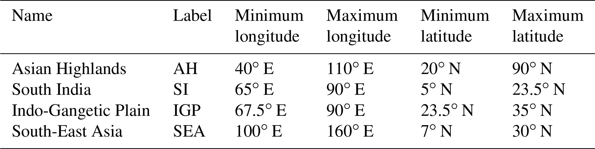
Table A2The maritime source regions are defined by the overlap of longitudinally and latitudinally restricted boxes with the seas.
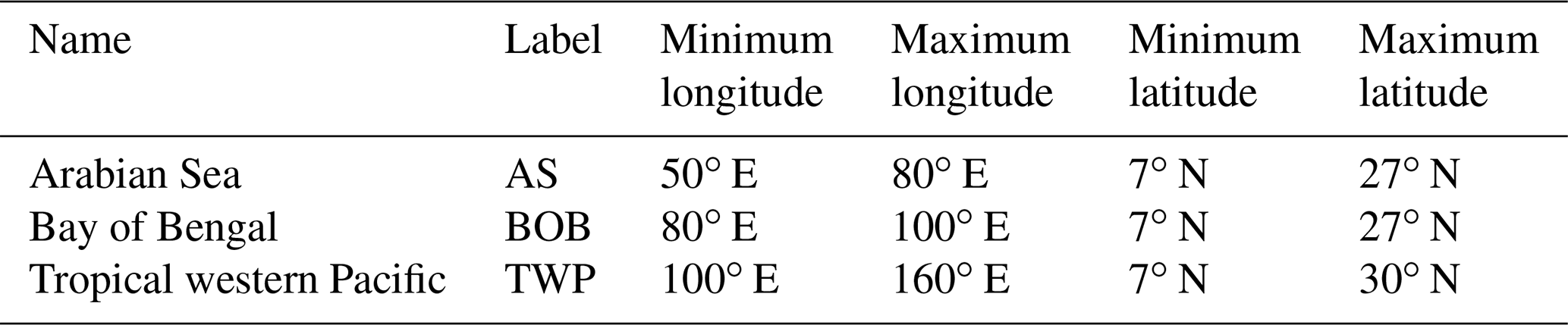
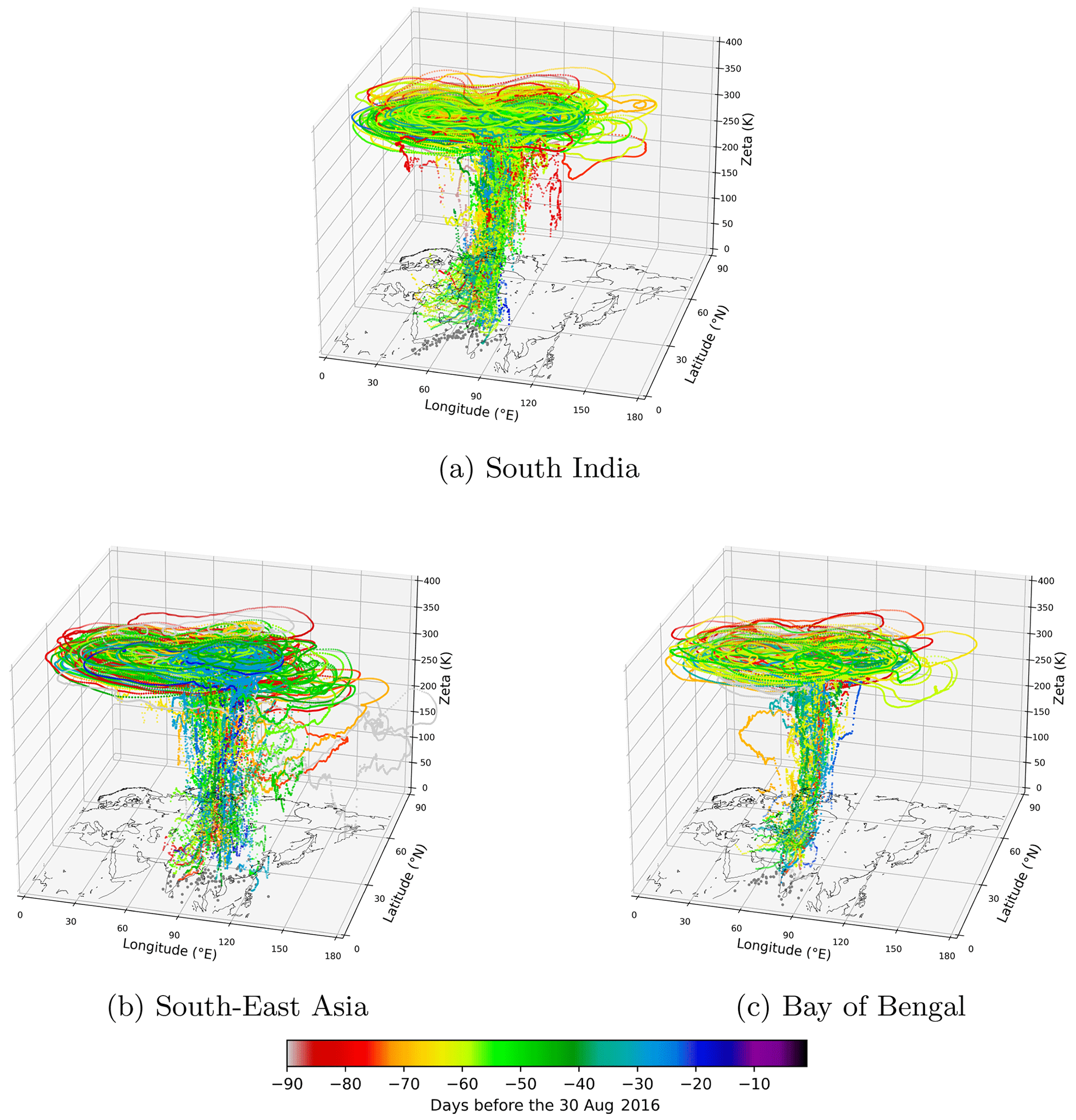
Figure B1Exemplary backward trajectories of air parcels of all of the 15 measurement days from the ATAL measurement to the MBL, categorised by the source region. Colours are chosen as in Fig. 1.
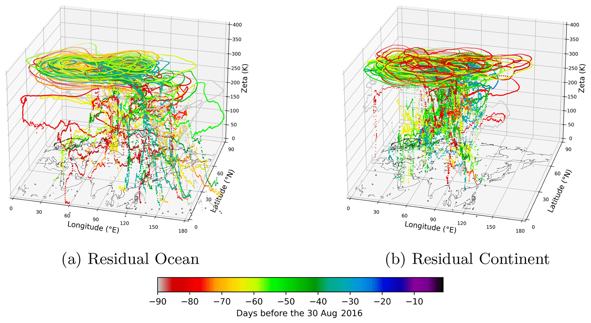
Figure B2Exemplary backward trajectories of air parcels of all of the 15 measurement days from the ATAL measurement to the MBL, categorised by the source region. Colours indicate the time when the air parcels leaves the MBL. Grey dots at the bottom show the horizontal position of the APs 48 h before they cross the MBL from below.
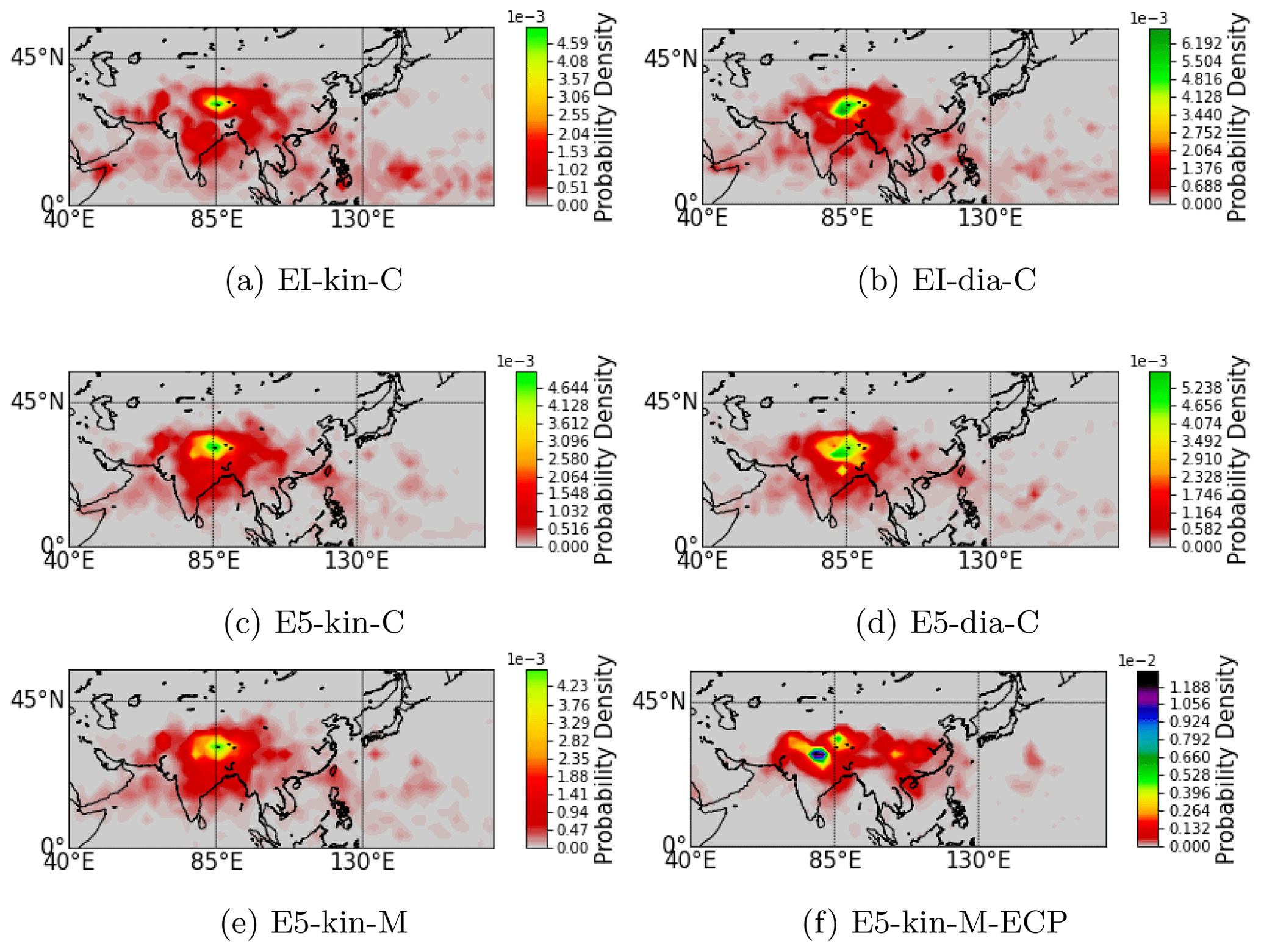
Figure C1PDFs for the MBL source region for some scenarios.
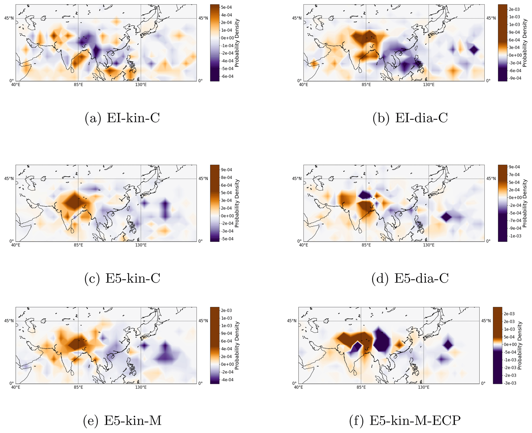
Figure D1PDF differences for days with high and low ATAL backscatter for specific scenarios, similar to Fig. 7a, illustrating the sensitivity of the PDF differences to the chosen scenario.
Table E1Mean transport time from the MBL into the UTLS in days, determined by the difference between the leaving time at the MBL and the arrival time above 340 K. Abbreviations are as defined in Tables A1 and A2. The residual ocean (Res. Oc.) and residual continent (Res. Cont.) describe the remaining maritime and continental regions that are not included in the definitions.
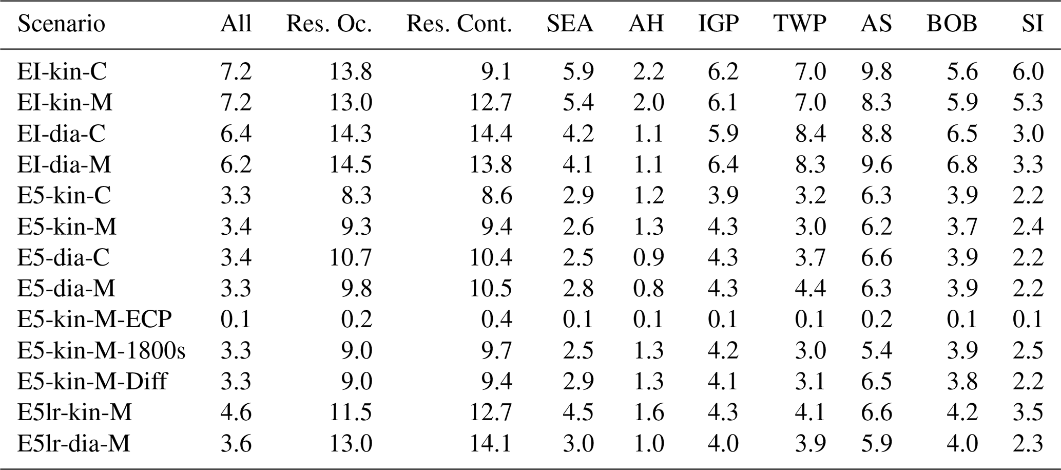
Table E2Median transport time from the MBL into the UTLS in days, determined by the difference between the leaving time at the MBL and the arrival time above 340 K. Abbreviations are as defined in Tables A1 and A2. The residual ocean (Res. Oc.) and residual continent (Res. Cont.) describe the remaining maritime and continental regions that are not included in the definitions.
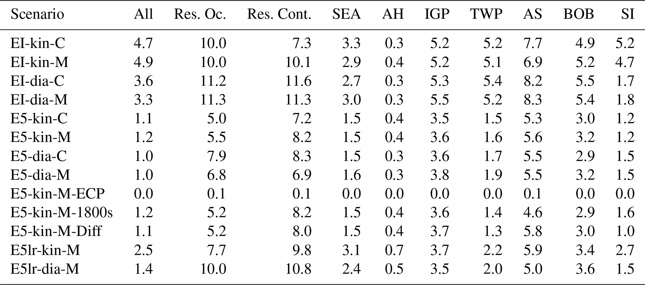
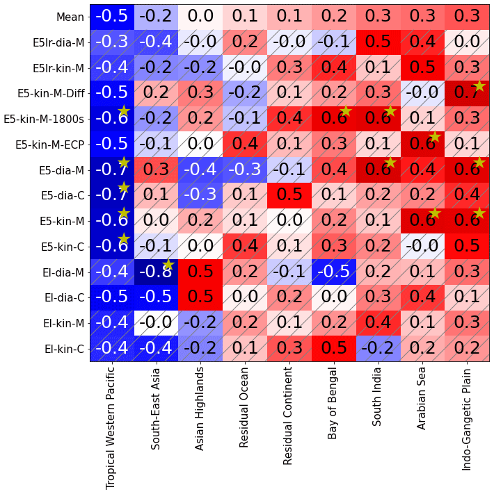
Figure E1All Spearman correlation coefficients for the relation between the daily BSR and the contributions of different regions for different scenarios. Hatched areas indicate insignificant results (p value higher 0.10). Boxes with yellow stars indicate p values lower than 0.05. The regions are ordered according to the scenario mean, from lowest to highest correlations.
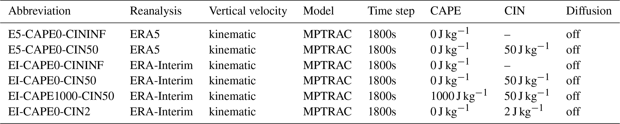
The default setting of the ECP in MPTRAC relies on a CAPE value of 0 J kg−1 as a threshold for triggering convection events. For our study, we found that the parameterisation can be improved to avoid spurious parameterised convection events over the Persian Gulf and the Red Sea. In these regions, extremely high convective inhibition, i.e. very stable low-level layers, prevent the release of the CAPE. Therefore, we implemented an additional threshold for CIN, which was set to 50 J kg−1 to remove unrealistic parameterised convection events over the Persian Gulf. Figure F1 illustrates the impact of the parameter choices of the convection parameterisation on the source identification for different threshold settings. E5-CAPE0-CIN50 is the same scenario as simulation E5-kin-M-ECP in other parts of the paper. Table F1 gives a detailed overview of the different set-ups of the convection parameterisation.
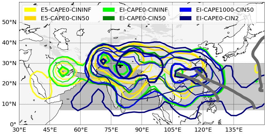
Figure F1The same as in Fig. 4 but for simulations with varying settings of the ECP parameters CIN and CAPE. E5-CAPE0-CIN50 is the same as simulation E5-kin-M-ECP.
Table F1Overview over scenarios, with different set-ups of the convection parameterisation, of 90 d backward calculations performed for the ATAL measurements above Nainital in August 2016. The abbreviation for each scenario contains the reanalysis in the first position, the CAPE threshold in the second position and the CIN threshold in the third position.
The ERA-Interim and ERA5 reanalysis data are available from the ECMWF (https://doi.org/10.24381/cds.adbb2d47, Hersbach et al., 2018). The CLaMS code can be accessed at the Jülich GitLab server: https://jugit.fz-juelich.de/clams/ (FZ Jülich, 2021). MPTRAC can be accessed under the terms of the GNU General Public License at https://doi.org/10.5281/zenodo.10067751 (Hoffmann et al., 2023a). We made use of the Japanese best-track data of typhoons for the analysis of the relation between tropical storms and the transport pathways (https://www.jma.go.jp/jma/jma-eng/jma-center/rsmc-hp-pub-eg/besttrack.html, Japan Meteorological Agency, 2020). Balloon sounding data will be provided on request by Suvarna Fadnavis (suvarna@tropmet.res.in).
The initial idea for this study came from BV and LH. The formal analysis, programming and further investigations were done by JC. BV, LH, NT and SG supervised the work and gave support with data and software. The writing was done by JC. The co-authors contributed with review and comments.
At least one of the (co-)authors is a member of the editorial board of Atmospheric Chemistry and Physics. The peer-review process was guided by an independent editor, and the authors also have no other competing interests to declare.
Publisher’s note: Copernicus Publications remains neutral with regard to jurisdictional claims made in the text, published maps, institutional affiliations, or any other geographical representation in this paper. While Copernicus Publications makes every effort to include appropriate place names, the final responsibility lies with the authors.
The authors gratefully acknowledge Simone Brunamonti, Teresa Jorge, Sreeharsha Hanumanthu, Peter Ölsner, Manish Naja, Bhupendra Bahadur Singh, Kunchala Ravi Kumar, Sunil Sonbawne, Hannu Jauhiainen, Holger Vömel, Frank G. Wienhold and Ruud Dirkson for conducting the measurements in Nainital and for providing the data. The work presented includes contributions to the NSFC–DFG 2020 project ATALtrack (VO 1276/6-1). This research has been supported by the HelmholtzAssociation of German Research Centres (HGF) through the projects Pilot Lab Exascale Earth System Modelling (PL-ExaESM) and Joint Lab Exascale Earth System Modelling (JL-ExaESM). We acknowledge the Jülich Supercomputing Centre for providing computing time and storage resources on the JUWELS supercomputer. Jan Clemens was partly funded by Helmholtz Interdisciplinary Doctoral Training in Energy and Climate Research (HITEC). We thank the Japan Meteorological Agency for providing the typhoon track data. We also thank the ECMWF for providing access to the ERA5 and ERA-Interim reanalysis data.
The article processing charges for this open-access publication were covered by the Forschungszentrum Jülich.
This paper was edited by Barbara Ervens and reviewed by two anonymous referees.
Appel, O., Köllner, F., Dragoneas, A., Hünig, A., Molleker, S., Schlager, H., Mahnke, C., Weigel, R., Port, M., Schulz, C., Drewnick, F., Vogel, B., Stroh, F., and Borrmann, S.: Chemical analysis of the Asian tropopause aerosol layer (ATAL) with emphasis on secondary aerosol particles using aircraft-based in situ aerosol mass spectrometry, Atmos. Chem. Phys., 22, 13607–13630, https://doi.org/10.5194/acp-22-13607-2022, 2022. a, b
Bergman, J. W., Jensen, E. J., Pfister, L., and Yang, Q.: Seasonal differences of vertical-transport efficiency in the tropical tropopause layer: On the interplay between tropical deep convection, large-scale vertical ascent, and horizontal circulations, J. Geophys. Res., 117, D05302, https://doi.org/10.1029/2011JD016992, 2012. a, b, c
Bossolasco, A., Jegou, F., Sellitto, P., Berthet, G., Kloss, C., and Legras, B.: Global modeling studies of composition and decadal trends of the Asian Tropopause Aerosol Layer, Atmos. Chem. Phys., 21, 2745–2764, https://doi.org/10.5194/acp-21-2745-2021, 2021. a
Brabec, M., Wienhold, F. G., Luo, B. P., Vömel, H., Immler, F., Steiner, P., Hausammann, E., Weers, U., and Peter, T.: Particle backscatter and relative humidity measured across cirrus clouds and comparison with microphysical cirrus modelling, Atmos. Chem. Phys., 12, 9135–9148, https://doi.org/10.5194/acp-12-9135-2012, 2012. a
Brunamonti, S., Jorge, T., Oelsner, P., Hanumanthu, S., Singh, B. B., Kumar, K. R., Sonbawne, S., Meier, S., Singh, D., Wienhold, F. G., Luo, B. P., Boettcher, M., Poltera, Y., Jauhiainen, H., Kayastha, R., Karmacharya, J., Dirksen, R., Naja, M., Rex, M., Fadnavis, S., and Peter, T.: Balloon-borne measurements of temperature, water vapor, ozone and aerosol backscatter on the southern slopes of the Himalayas during StratoClim 2016–2017, Atmos. Chem. Phys., 18, 15937–15957, https://doi.org/10.5194/acp-18-15937-2018, 2018. a, b
Bucci, S., Legras, B., Sellitto, P., D'Amato, F., Viciani, S., Montori, A., Chiarugi, A., Ravegnani, F., Ulanovsky, A., Cairo, F., and Stroh, F.: Deep-convective influence on the upper troposphere–lower stratosphere composition in the Asian monsoon anticyclone region: 2017 StratoClim campaign results, Atmos. Chem. Phys., 20, 12193–12210, https://doi.org/10.5194/acp-20-12193-2020, 2020. a, b, c, d, e, f
Bucholtz, A.: Rayleigh-scattering calculations for the terrestrial atmosphere, Appl. Optics, 34, 2765–2773, https://doi.org/10.1364/AO.34.002765, 1995. a
Dee, D. P., Uppala, S. M., Simmons, A. J., Berrisford, P., Poli, P., Kobayashi, S., Andrae, U., Balmaseda, M. A., Balsamo, G., Bauer, P., Bechtold, P., Beljaars, A. C. M., van de Berg, L., Bidlot, J., Bormann, N., Delsol, C., Dragani, R., Fuentes, M., Geer, A. J., Haimberger, L., Healy, S. B., Hersbach, H., Hólm, E. V., Isaksen, L., Kållberg, P., Köhler, M., Matricardi, M., McNally, A. P., Monge-Sanz, B. M., Morcrette, J.-J., Park, B.-K., Peubey, C., de Rosnay, P., Tavolato, C., Thépaut, J.-N., and Vitart, F.: The ERA-Interim reanalysis: configuration and performance of the data assimilation system, Q. J. Roy. Meteor. Soc., 137, 553–597, https://doi.org/10.1002/qj.828, 2011. a, b
Fadnavis, S., Semeniuk, K., Pozzoli, L., Schultz, M. G., Ghude, S. D., Das, S., and Kakatkar, R.: Transport of aerosols into the UTLS and their impact on the Asian monsoon region as seen in a global model simulation, Atmos. Chem. Phys., 13, 8771–8786, https://doi.org/10.5194/acp-13-8771-2013, 2013. a
Fadnavis, S., Kalita, G., Kumar, K. R., Gasparini, B., and Li, J.-L. F.: Potential impact of carbonaceous aerosol on the upper troposphere and lower stratosphere (UTLS) and precipitation during Asian summer monsoon in a global model simulation, Atmos. Chem. Phys., 17, 11637–11654, https://doi.org/10.5194/acp-17-11637-2017, 2017. a
Fairlie, T. D., Liu, H., Vernier, J.-P., Campuzano-Jost, P., Jimenez, J. L., Jo, D. S., Zhang, B., Natarajan, M., Avery, M. A., and Huey, G.: Estimates of Regional Source Contributions to the Asian Tropopause Aerosol Layer Using a Chemical Transport Model, J. Geophys. Res.-Atmos., 125, e2019JD031506, https://doi.org/10.1029/2019JD031506, 2020. a
FZ Jülich: CLaMS, GitLab archive [code], https://jugit.fz-juelich.de/clams/, last access: 1 January 2021. a
Gerbig, C., Lin, J. C., Wofsy, S. C., Daube, B. C., Andrews, A. E., Stephens, B. B., Bakwin, P. S., and Grainger, C. A.: Toward constraining regional-scale fluxes of CO2 with atmospheric observations over a continent: 2. Analysis of COBRA data using a receptor-oriented framework, J. Geophys. Res., 108, 4757, https://doi.org/10.1029/2003JD003770, 2003. a
Gottschaldt, K.-D., Schlager, H., Baumann, R., Cai, D. S., Eyring, V., Graf, P., Grewe, V., Jöckel, P., Jurkat-Witschas, T., Voigt, C., Zahn, A., and Ziereis, H.: Dynamics and composition of the Asian summer monsoon anticyclone, Atmos. Chem. Phys., 18, 5655–5675, https://doi.org/10.5194/acp-18-5655-2018, 2018. a
Hanumanthu, S., Vogel, B., Müller, R., Brunamonti, S., Fadnavis, S., Li, D., Ölsner, P., Naja, M., Singh, B. B., Kumar, K. R., Sonbawne, S., Jauhiainen, H., Vömel, H., Luo, B., Jorge, T., Wienhold, F. G., Dirkson, R., and Peter, T.: Strong day-to-day variability of the Asian Tropopause Aerosol Layer (ATAL) in August 2016 at the Himalayan foothills, Atmos. Chem. Phys., 20, 14273–14302, https://doi.org/10.5194/acp-20-14273-2020, 2020. a, b, c, d, e, f, g, h, i, j, k, l, m, n, o, p, q, r, s, t, u, v, w, x
Hersbach, H., Bell, B., Berrisford, P., Biavati, G., Horányi, A., Muñoz Sabater, J., Nicolas, J., Peubey, C., Radu, R., Rozum, I., Schepers, D., Simmons, A., Soci, C., Dee, D., and Thépaut, J.-N.: ERA5 hourly data on single levels from 1940 to present, Copernicus Climate Change Service (C3S) Climate Data Store (CDS) [data set], https://doi.org/10.24381/cds.adbb2d47, 2018. a
Hersbach, H., Bell, B., Berrisford, P., Hirahara, S., Horányi, A., Muñoz-Sabater, J., Nicolas, J., Peubey, C., Radu, R., Schepers, D., Simmons, A., Soci, C., Abdalla, S., Abellan, X., Balsamo, G., Bechtold, P., Biavati, G., Bidlot, J., Bonavita, M., De Chiara, G., Dahlgren, P., Dee, D., Diamantakis, M., Dragani, R., Flemming, J., Forbes, R., Fuentes, M., Geer, A., Haimberger, L., Healy, S., Hogan, R. J., Hólm, E., Janisková, M., Keeley, S., Laloyaux, P., Lopez, P., Lupu, C., Radnoti, G., de Rosnay, P., Rozum, I., Vamborg, F., Villaume, S., and Thépaut, J.-N.: The ERA5 global reanalysis, Q. J. Roy. Meteor. Soc., 146, 1999–2049, https://doi.org/10.1002/qj.3803, 2020. a, b
Hoffmann, L., Rößler, T., Griessbach, S., Heng, Y., and Stein, O.: Lagrangian transport simulations of volcanic sulfur dioxide emissions: impact of meteorological data products, J. Geophys. Res., 121, 4651–4673, https://doi.org/10.1002/2015JD023749, 2016. a
Hoffmann, L., Günther, G., Li, D., Stein, O., Wu, X., Griessbach, S., Heng, Y., Konopka, P., Müller, R., Vogel, B., and Wright, J. S.: From ERA-Interim to ERA5: the considerable impact of ECMWF's next-generation reanalysis on Lagrangian transport simulations, Atmos. Chem. Phys., 19, 3097–3124, https://doi.org/10.5194/acp-19-3097-2019, 2019. a, b, c
Hoffmann, L., Baumeister, P. F., Cai, Z., Clemens, J., Griessbach, S., Günther, G., Heng, Y., Liu, M., Haghighi Mood, K., Stein, O., Thomas, N., Vogel, B., Wu, X., and Zou, L.: Massive-Parallel Trajectory Calculations version 2.2 (MPTRAC-2.2): Lagrangian transport simulations on graphics processing units (GPUs), Geosci. Model Dev., 15, 2731–2762, https://doi.org/10.5194/gmd-15-2731-2022, 2022. a, b
Hoffmann, L., Clemens, J., Griessbach, S., Haghighi Mood, K., Khosrawi, F., Liu, M., Lu, Y.-S., Sonnabend, J., and Zou, L.: Massive-Parallel Trajectory Calculations (MPTRAC), Version v2.6, Zenodo [code], https://doi.org/10.5281/zenodo.10067751, 2023a. a
Hoffmann, L., Konopka, P., Clemens, J., and Vogel, B.: Lagrangian transport simulations using the extreme convection parameterization: an assessment for the ECMWF reanalyses, Atmos. Chem. Phys., 23, 7589–7609, https://doi.org/10.5194/acp-23-7589-2023, 2023b. a
Honomichl, S. B. and Pan, L. L.: Transport From the Asian Summer Monsoon Anticyclone Over the Wesetrn Pacific, J. Geophys. Res.-Atmos., 125, e2019JD032094, https://doi.org/10.1029/2019JD032094, 2020. a
Höpfner, M., Ungermann, J., Borrmann, S., Wagner, R., Spang, R., Riese, M., Stiller, G., Appel, O., Batenburg, A. M., Bucci, S., Cairo, F., Dragoneas, A., Friedl-Vallon, F., Hünig, A., Johansson, S., Krasauskas, L., Legras, B., Leisner, T., Mahnke, C., Möhler, O., Molleker, S., Müller, R., Neubert, T., Orphal, J., Preusse, P., Rex, M., Saathoff, H., Stroh, F., Weigel, R., and Wohltmann, I.: Ammonium nitrate particles formed in upper troposphere from ground ammonia sources during Asian monsoons, Nat. Geosci., 12, 608–612, https://doi.org/10.1038/s41561-019-0385-8, 2019. a, b, c, d, e, f
Japan Meteorological Agency (JMA): Typhoon tracks, RSMC Tokyo – Typhoon Center [data set], https://www.jma.go.jp/jma/jma-eng/jma-center/rsmc-hp-pub-eg/besttrack.html, last access: 5 October 2020. a
Johansson, S., Höpfner, M., Kirner, O., Wohltmann, I., Bucci, S., Legras, B., Friedl-Vallon, F., Glatthor, N., Kretschmer, E., Ungermann, J., and Wetzel, G.: Pollution trace gas distributions and their transport in the Asian monsoon upper troposphere and lowermost stratosphere during the StratoClim campaign 2017, Atmos. Chem. Phys., 20, 14695–14715, https://doi.org/10.5194/acp-20-14695-2020, 2020. a
Kim, Y.-S., Shibata, T., Iwasaka, Y., Shi, G., Zhou, X., Tamura, K., and Ohashi, T.: Enhancement of aerosols near the cold tropopause in summer over Tibetan Plateau: lidar and balloonborne measurements in 1999 at Lhasa, Tibet, China, in: Lidar Remote Sensing for Industry and Environment Monitoring III, edited by Singh, U. N., Itabe, T., and Liu, Z., International Society for Optics and Photonics, SPIE, vol. 4893, 496–503, https://doi.org/10.1117/12.466090, 2003. a
Kuttippurath, J., Singh, A., Dash, S. P., Mallick, N., Clerbaux, C., Van Damme, M., Clarisse, L., Coheur, P. F., Raj, S., Abbhishek, K., and Varikoden, H.: Record high levels of atmospheric ammonia over India: Spatial and temporal analyses, Sci. Total Environ., 740, 139986, https://doi.org/10.1016/j.scitotenv.2020.139986, 2020. a
Legras, B. and Bucci, S.: Confinement of air in the Asian monsoon anticyclone and pathways of convective air to the stratosphere during the summer season, Atmos. Chem. Phys., 20, 11045–11064, https://doi.org/10.5194/acp-20-11045-2020, 2020. a, b, c, d
Li, D., Vogel, B., Bian, J., Müller, R., Pan, L. L., Günther, G., Bai, Z., Li, Q., Zhang, J., Fan, Q., and Vömel, H.: Impact of typhoons on the composition of the upper troposphere within the Asian summer monsoon anticyclone: the SWOP campaign in Lhasa 2013, Atmos. Chem. Phys., 17, 4657–4672, https://doi.org/10.5194/acp-17-4657-2017, 2017. a, b, c, d
Li, D., Vogel, B., Müller, R., Bian, J., Günther, G., Ploeger, F., Li, Q., Zhang, J., Bai, Z., Vömel, H., and Riese, M.: Dehydration and low ozone in the tropopause layer over the Asian monsoon caused by tropical cyclones: Lagrangian transport calculations using ERA-Interim and ERA5 reanalysis data, Atmos. Chem. Phys., 20, 4133–4152, https://doi.org/10.5194/acp-20-4133-2020, 2020. a, b, c, d, e, f, g, h, i, j, k
Loughner, C. P., Fasoli, B., Stein, A. F., and Lin, J. C.: Incorporating Features from the Stochastic Time-Inverted Lagrangian Transport (STILT) Model into the Hybrid Single-Particle Lagrangian Integrated Trajectory (HYSPLIT) Model: A Unified Dispersion Model for Time-Forward and Time-Reversed Applications, J. Appl. Meteorol. Clim., 60, 799–810, https://doi.org/10.1175/JAMC-D-20-0158.1, 2021. a
Mahowald, N. M., Plumb, R. A., Rasch, P. J., del Corral, J., Sassi, F., and Heres, W.: Stratospheric transport in a three-dimensional isentropic coordinate model, J. Geophys. Res.-Atmos., 107, ACH 3-1–ACH 3-14, https://doi.org/10.1029/2001JD001313, 2002. a
Malakar, P., Kesarkar, A., Bhate, J., Singh, V., and Deshamukhya, A.: Comparison of Reanalysis Data Sets to Comprehend the Evolution of Tropical Cyclones Over North Indian Ocean, Earth Space Sci., 7, e2019EA000978, https://doi.org/10.1029/2019EA000978, 2020. a
Manney, G. L., Santee, M. L., Lawrence, Z. D., Wargan, K., and Schwartz, M. J.: A Moments View of Climatology and Variability of the Asian Summer Monsoon Anticyclone, J. Climate, 34, 7821–7841, https://doi.org/10.1175/JCLI-D-20-0729.1, 2021. a
McKenna, D. S., Grooß, J.-U., Günther, G., Konopka, P., Müller, R., Carver, G., and Sasano, Y.: A new Chemical Lagrangian Model of the Stratosphere (CLaMS) 2. Formulation of chemistry scheme and initialization, J. Geophys. Res.-Atmos., 107, ACH 4-1–ACH 4-14, https://doi.org/10.1029/2000JD000113, 2002a. a
McKenna, D. S., Konopka, P., Grooß, J.-U., Günther, G., Müller, R., Spang, R., Offermann, D., and Orsolini, Y.: A new Chemical Lagrangian Model of the Stratosphere (CLaMS) 1. Formulation of advection and mixing, J. Geophys. Res.-Atmos., 107, ACH 15-1–ACH 15-15, https://doi.org/10.1029/2000JD000114, 2002b. a
Nützel, M., Dameris, M., and Garny, H.: Movement, drivers and bimodality of the South Asian High, Atmos. Chem. Phys., 16, 14755–14774, https://doi.org/10.5194/acp-16-14755-2016, 2016. a
Ploeger, F., Konopka, P., Günther, G., Grooß, J.-U., and Müller, R.: Impact of the vertical velocity scheme on modeling transport across the tropical tropopause layer, J. Geophys. Res., 115, D03301, https://doi.org/10.1029/2009JD012023, 2010. a, b, c, d
Ploeger, F., Fueglistaler, S., Grooß, J.-U., Günther, G., Konopka, P., Liu, Y. S., Müller, R., Ravegnani, F., Schiller, C., Ulanovski, A., and Riese, M.: Insight from ozone and water vapour on transport in the tropical tropopause layer (TTL), Atmos. Chem. Phys., 11, 407–419, https://doi.org/10.5194/acp-11-407-2011, 2011. a
Ploeger, F., Diallo, M., Charlesworth, E., Konopka, P., Legras, B., Laube, J. C., Grooß, J.-U., Günther, G., Engel, A., and Riese, M.: The stratospheric Brewer–Dobson circulation inferred from age of air in the ERA5 reanalysis, Atmos. Chem. Phys., 21, 8393–8412, https://doi.org/10.5194/acp-21-8393-2021, 2021. a, b
Pommrich, R., Müller, R., Grooß, J.-U., Konopka, P., Ploeger, F., Vogel, B., Tao, M., Hoppe, C. M., Günther, G., Spelten, N., Hoffmann, L., Pumphrey, H.-C., Viciani, S., D'Amato, F., Volk, C. M., Hoor, P., Schlager, H., and Riese, M.: Tropical troposphere to stratosphere transport of carbon monoxide and long-lived trace species in the Chemical Lagrangian Model of the Stratosphere (CLaMS), Geosci. Model Dev., 7, 2895–2916, https://doi.org/10.5194/gmd-7-2895-2014, 2014. a, b
Rößler, T., Stein, O., Heng, Y., Baumeister, P., and Hoffmann, L.: Trajectory errors of different numerical integration schemes diagnosed with the MPTRAC advection module driven by ECMWF operational analyses, Geosci. Model Dev., 11, 575–592, https://doi.org/10.5194/gmd-11-575-2018, 2018. a
Stohl, A., Forster, C., Frank, A., Seibert, P., and Wotawa, G.: Technical note: The Lagrangian particle dispersion model FLEXPART version 6.2, Atmos. Chem. Phys., 5, 2461–2474, https://doi.org/10.5194/acp-5-2461-2005, 2005. a
Taszarek, M., Pilguj, N., Allen, J. T., Gensini, V., Brooks, H. E., and Szuster, P.: Comparison of convective parameters derived from ERA5 and MERRA2 with rawinsonde data over Europe and North America, J. Climate, 34, 3211–3237, https://doi.org/10.1175/JCLI-D-20-0484.1, 2020. a, b
Thomason, L. W. and Vernier, J.-P.: Improved SAGE II cloud/aerosol categorization and observations of the Asian tropopause aerosol layer: 1989–2005, Atmos. Chem. Phys., 13, 4605–4616, https://doi.org/10.5194/acp-13-4605-2013, 2013. a
Tobo, Y., Iwasaka, Y., Shi, G.-Y., Kim, Y.-S., Ohashi, T., Tamura, K., and Zhang, D.: Balloon-borne observations of high aerosol concentrations near the summertime tropopause over the Tibetan Plateau, Atmos. Res., 84, 233–241, https://doi.org/10.1016/j.atmosres.2006.08.003, 2007. a
Vernier, J.-P., Thomason, L. W., and Kar, J.: CALIPSO detection of an Asian tropopause aerosol layer, Geophys. Res. Lett., 38, L07804, https://doi.org/10.1029/2010GL046614, 2011. a, b, c, d
Vernier, J.-P., Fairlie, T. D., Deshler, T., Ratnam, M. V., Gadhavi, H., Kumar, B. S., Natarajan, M., Pandit, A. K., Raj, S. T. A., Kumar, A. H., Jayaraman, A., Singh, A. K., Rastogi, N., Sinha, P. R., Kumar, S., Tiwari, S., Wegner, T., Baker, N., Vignelles, D., Stenchikov, G., Shevchenko, I., Smith, J., Bedka, K., Kesarkar, A., Singh, V., Bhate, J., Ravikiran, V., Rao, M. D., Ravindrababu, S., Patel, A., Vernier, H., Wienhold, F. G., Liu, H., Knepp, T. N., Thomason, L., Crawford, J., Ziemba, L., Moore, J., Crumeyrolle, S., Williamson, M., Berthet, G., Jégou, F., and Renard, J.-B.: BATAL: The Balloon Measurement Campaigns of the Asian Tropopause Aerosol Layer, B. Am. Meteorol. Soc., 99, 955–973, https://doi.org/10.1175/BAMS-D-17-0014.1, 2018. a, b, c
Vogel, B., Günther, G., Müller, R., Grooß, J.-U., Hoor, P., Krämer, M., Müller, S., Zahn, A., and Riese, M.: Fast transport from Southeast Asia boundary layer sources to northern Europe: rapid uplift in typhoons and eastward eddy shedding of the Asian monsoon anticyclone, Atmos. Chem. Phys., 14, 12745–12762, https://doi.org/10.5194/acp-14-12745-2014, 2014. a
Vogel, B., Günther, G., Müller, R., Grooß, J.-U., and Riese, M.: Impact of different Asian source regions on the composition of the Asian monsoon anticyclone and of the extratropical lowermost stratosphere, Atmos. Chem. Phys., 15, 13699–13716, https://doi.org/10.5194/acp-15-13699-2015, 2015. a
Vogel, B., Müller, R., Günther, G., Spang, R., Hanumanthu, S., Li, D., Riese, M., and Stiller, G. P.: Lagrangian simulations of the transport of young air masses to the top of the Asian monsoon anticyclone and into the tropical pipe, Atmos. Chem. Phys., 19, 6007–6034, https://doi.org/10.5194/acp-19-6007-2019, 2019. a, b, c
Weigel, R., Mahnke, C., Baumgartner, M., Dragoneas, A., Vogel, B., Ploeger, F., Viciani, S., D'Amato, F., Bucci, S., Legras, B., Luo, B., and Borrmann, S.: In situ observation of new particle formation (NPF) in the tropical tropopause layer of the 2017 Asian monsoon anticyclone – Part 1: Summary of StratoClim results, Atmos. Chem. Phys., 21, 11689–11722, https://doi.org/10.5194/acp-21-11689-2021, 2021. a
Yongfu, Q., Qiong, Z., Yonghong, Y., and Xuehong, Z.: Seasonal variation and heat preference of the south asia high, Adv. Atmos. Sci., 19, 821–836, https://doi.org/10.1007/s00376-002-0047-3, 2002. a
Zhang, J., Liu, Y., Chen, H., Cai, Z., Bai, Z., Ran, L., Luo, T., Yang, J., Wang, Y., Xuan, Y., Huang, Y., Wu, X., Bian, J., and Lu, D.: A multi-location joint field observation of the stratosphere and troposphere over the Tibetan Plateau, Earth Planet. Phys., 3, 87–92, https://doi.org/10.26464/epp2019017, 2019a. a, b
Zhang, J., Wu, X., Liu, S., Bai, Z., Xia, X., Chen, B., Zong, X., and Bian, J.: In situ measurements and backward-trajectory analysis of high-concentration, fine-mode aerosols in the UTLS over the Tibetan Plateau, Environ. Res. Lett., 14, 124068, https://doi.org/10.1088/1748-9326/ab5a9f, 2019b. a, b, c
Zhang, J., Wu, X., Bian, J., Xia, X., Bai, Z., Liu, Y., Cai, Z., Huo, J., and Lyu, D.: Aerosol variations in the upper troposphere and lower stratosphere over the Tibetan Plateau, Environ. Res. Lett., 15, 094068, https://doi.org/10.1088/1748-9326/ab9b43, 2020. a, b
- Abstract
- Introduction
- Data and methods
- Results
- Discussion and conclusions
- Appendix A: Definition of source regions
- Appendix B: Transport pathways from source regions
- Appendix C: PDF for different scenarios
- Appendix D: PDF differences for different scenarios
- Appendix E: Correlation to all regions
- Appendix F: Sensitivity tests for simulations employing the extreme convection parameterisation (ECP)
- Code and data availability
- Author contributions
- Competing interests
- Disclaimer
- Acknowledgements
- Financial support
- Review statement
- References