Deep-learning-derived planetary boundary layer height from conventional meteorological measurements

The planetary boundary layer (PBL) height (PBLH) is an important parameter for various meteorological and climate studies. This study presents a multi-structure deep neural network (DNN) model, which can estimate PBLH by integrating the morning temperature profiles and surface meteorological observations. The DNN model is developed by leveraging a rich dataset of PBLH derived from long-standing radiosonde records augmented with high-resolution micro-pulse lidar and Doppler lidar observations. We access the performance of the DNN with an ensemble of 10 members, each featuring distinct hidden-layer structures, which collectively yield a robust 27-year PBLH dataset over the southern Great Plains from 1994 to 2020. The influence of various meteorological factors on PBLH is rigorously analyzed through the importance test. Moreover, the DNN model's accuracy is evaluated against radiosonde observations and juxtaposed with conventional remote sensing methodologies, including Doppler lidar, ceilometer, Raman lidar, and micro-pulse lidar. The DNN model exhibits reliable performance across diverse conditions and demonstrates lower biases relative to remote sensing methods. In addition, the DNN model, originally trained over a plain region, demonstrates remarkable adaptability when applied to the heterogeneous terrains and climates encountered during the GoAmazon (Green Ocean Amazon; tropical rainforest) and CACTI (Cloud, Aerosol, and Complex Terrain Interactions; middle-latitude mountain) campaigns. These findings demonstrate the effectiveness of deep learning models in estimating PBLH, enhancing our understanding of boundary layer processes with implications for improving the representation of PBL in weather forecasting and climate modeling.

1 Introduction

The planetary boundary layer (PBL) is the atmosphere's lowest part, where Earth's surface directly influences meteorological variables, impacting the climate system (Garratt, 1994; Kaimal and Finnigan, 1994). The PBL height (PBLH) is a meteorological factor that strongly influences surface–atmosphere exchanges of heat, moisture, and energy (Stull, 1988; Caughey, 1984; Holtslag and Nieuwstadt, 1986; Mahrt, 1999; Helbig et al., 2021; Guo et al., 2024; Beamesderfer et al., 2022). In addition, PBLH is a crucial variable for monitoring and simulating surface pollutant behaviors since it determines the volume available for near-surface pollutant dispersion (Li et al., 2017; Su et al., 2024a; Tucker et al., 2009; Wang et al., 2020). Due to its impact on cloud evolution and the development of convective systems, PBLH is also a key parameter in numerical weather forecasts and climate projections (Deardorff, 1970; Kaimal et al., 1976; Menut et al., 1999; Park et al., 2001; Emanuel, 1994; Guo et al., 2017, 2019; Lilly, 1968; Matsui et al., 2004).

Radiosonde (SONDE) measurements remain the standard method for estimating PBLH, yet they are hampered by limitations in temporal frequency, restricting its ability to capture the whole diurnal cycle of PBL development (Stull, 1988; Seidel et al., 2010; Guo et al., 2021; Liu and Liang, 2010). To overcome these challenges, there has been an increasing dependence on remote sensing techniques, especially lidar systems. These techniques capture atmospheric vertical information (e.g., aerosols, temperature, humidity, and wind) at high temporal and vertical resolutions, leading to remote-sensing-based retrievals of PBLH (Menut et al., 1999; Kotthaus et al., 2023; Sawyer and Li, 2013; Wang et al., 2023). The remote sensing systems, including Doppler lidar (Barlow et al., 2011), ceilometer (Zhang et al., 2022), Raman lidar (Summa et al., 2013), and micro-pulse lidar (Melfi et al., 1985), utilize laser-based technology to track PBLH diurnal evolutions, helping us understand the PBL evolutions (Cohn and Angevine, 2000; Davis et al., 2000). In addition, wind profilers can estimate PBLH using algorithms that analyze the signal-to-noise ratio from wind profiler data (Molod et al., 2015; Solanki et al., 2022; B. Liu et al., 2019; Salmun et al., 2023; Bianco and Wilczak, 2002; Bianco et al., 2008; Tao et al., 2021).

However, despite the advancement in remote sensing for the estimation of PBLH, challenges still remain in bridging the results obtained by different remote sensing instruments with those obtained from the SONDE measurements (Zhang et al., 2022; Chu et al., 2019). Specifically, interpreting aerosol, turbulence, and moisture profiles derived from remote sensing techniques to determine PBLH bears inherent limitations due to the unstable signal-to-noise ratio (Kotthaus et al., 2023; Krishnamurthy et al., 2021). This issue is compounded by the different measurement methodologies and definitions employed by various remote sensing tools, leading to uncertainties when comparing their PBLH estimates to the retrievals derived from SONDE measurements (Zhang et al., 2022; Sawyer and Li, 2013).

As machine learning (ML) has shown potential in atmospheric science (McGovern et al., 2017; Gagne et al., 2019; Su et al., 2020a; Vassallo et al., 2020; Cadeddu et al., 2009; Molero et al., 2022), this technique presents a promising tool for refining the estimation of PBLH to resolve the inherent complexity and variability in PBL. For example, several studies use ML to identify PBLH using thermodynamic profiles of the Atmospheric Emitted Radiance Interferometer (AERI) or using backscatter profiles from lidar, highlighting ML's superiority over conventional techniques under different scenarios (Sleeman et al., 2020; Rieutord et al., 2021; Liu et al., 2022; Ye et al., 2021). For example, Li et al. (2023) applied an ML algorithm for retrieving PBLH under complex atmospheric conditions accounting for the vertical distribution of aerosols. Krishnamurthy et al. (2021) incorporated a random forest model, along with machine learning, to use Doppler lidar data for the extraction of PBLH with better results compared to the results retrieved by traditional methods.

While existing ML methodologies have made great progress in estimating PBLH, these studies mainly focus on refining retrievals from remote sensing data, particularly lidar-based technologies. Thus, there is an inherent limitation to the applicability due to a reliance on specific remote sensing instruments. To address this issue, we aim to leverage and integrate the comprehensive field observations (i.e., radiosonde and remote sensing techniques) to develop a deep learning model for direct PBLH estimation from conventional meteorological data. This strategy circumvents the limitations of relying on particular remote sensing technologies. Furthermore, our model employs an advanced deep neural network (DNN) approach (Sze et al., 2017; Schmidhuber, 2015; Nielsen, 2015; Pang et al., 2020), diverging from traditional ML methods like random forest. This deep learning model utilizes ensemble techniques, constructing arrays of various structures and using their average for the final estimation. This approach provides particular advantages in the context of complex and nonlinear processes (Ganaie et al., 2022; Mohammed and Kora, 2023). The ensemble DNN with multi-structure design shows very strong flexibility and robustness, so it performs relatively better and has high stability across a wide range of conditions (Xue et al., 2020; Dong et al., 2020). This facilitates the adaptability of the DNN as a tool for PBLH estimation, which can be utilized under different scenarios and locations.

By focusing on the interaction between surface meteorology and the PBL, this study introduces a DNN-based method to estimate the daytime evolution of PBLH from morning temperature profiles and surface meteorology. We evaluate the model's performance using extensive datasets over the southern Great Plains (SGP) for a period spanning 27 years (1994–2020) and include comparisons with PBLH estimations obtained from measurements of Doppler lidar, ceilometer, Raman lidar, and micro-pulse lidar. Furthermore, we explore the generalizability of the model to different geographic regions and climates, as tested during the field campaigns, e.g., Green Ocean Amazon (GoAmazon) and Cloud, Aerosol, and Complex Terrain Interactions (CACTI).

2 Data and instruments

2.1 ARM sites

The Atmospheric Radiation Measurement (ARM) program, funded by the U.S. Department of Energy, has been employed at the southern Great Plains (SGP) site in Oklahoma (36.607° N, 97.488° W), situated 314 m above mean sea level. This study use comprehensive field observations at the SGP site during 1994 to 2020. In addition to the SGP site, this study utilizes data from the ARM GoAmazon (3.213° S, 60.598° W) and ARM CACTI (32.126° S, 64.728° W) field campaigns to carry out independent tests for the deep learning model. Specifically, the GoAmazon campaign is located in the Amazon tropical forests and provides rich field observation data during 2014–2015 (Martin et al., 2016). Meanwhile, the CACTI central site, at an elevation of 1141 m within the Sierras de Córdoba mountain range in north-central Argentina, offers the observations during the 2018–2019 period (Varble et al., 2021). Utilizing these comprehensive ARM datasets, our study includes thermodynamic profiles derived from radiosondes, data from the Active Remote Sensing of Clouds dataset (ARSCL; Clothiaux et al., 2000, 2001; Kollias et al., 2020), in situ surface flux measurements, and standard meteorological observations at the surface, as documented by Cook (2018) and Xie et al. (2010).

SONDE measurements at the ARM sites routinely launch several times a day and provide detailed information on the thermodynamic conditions of the atmosphere. The technical details of the ARM SONDE data are documented in Holdridge et al. (2011). Moreover, we use the surface meteorological parameters at the standard meteorological station. In situ measurements at 2 m above ground level provide data on temperature, relative humidity, and vapor pressure. In addition, this study obtains the surface sensible and latent heat fluxes from the surface instruments (Wesely et al., 1995). In the SGP, we use the best-estimate surface fluxes in the bulk aerodynamic energy balance Bowen ratio (BAEBBR) product, which is derived from the measurements by the energy balance Bowen ratio (EBBR). Due to the availability, we utilize the surface fluxes from Quality Controlled Eddy Correlation Flux Measurement (QCECOR) datasets from the CACTI and GoAmazon sites (Tang et al., 2019).

2.2 Existing PBLH datasets over the ARM sites

For analyzing PBLH, we have utilized a variety of datasets to get a full picture of PBLH derived from different instruments. These datasets are developed using different methodologies and instruments and jointly offer detailed information about PBLH under various meteorological conditions. Among these datasets, SONDE- and ceilometer-derived PBLH is available for all three sites; other datasets are only available over the SGP. The technical details for these datasets can be found in the corresponding publications or technical reports.

1. SONDE-derived PBLH by Liu and Liang (2010). PBLHs are retrieved using a method developed by Liu and Liang (2010), based on potential temperature gradients from SONDE measurements. We focus on daytime data during 05:00–18:00 local time (LT), with a resampled vertical resolution of 5 hPa. The SONDE dataset is available at https://doi.org/10.5439/1595321.

2. Doppler-lidar-derived PBLH by Sivaraman and Zhang (2021). Doppler lidar PBLH estimates are derived using a vertical velocity variance method during 2010–2019 (Tucker et al., 2009; Lareau et al., 2018; Sivaraman and Zhang, 2021). The dataset is available at https://doi.org/10.5439/1726254.

3. Combined MPL–SONDE (micro-pulse lidar) PBLH by Su et al. (2020b). We utilize a PBLH dataset that merges lidar and SONDE measurements during 1998–2023, ensuring vertical coherence and temporal continuity (Su et al., 2020b). An additional method for handling cloudy conditions is detailed in Su et al. (2022). The dataset is available at https://doi.org/10.5439/2007149.

4. Ceilometer-derived PBLH by Zhang et al. (2022). The Vaisala CL31 ceilometer, with a 7.7 km vertical range, provides detailed backscatter profiles used for PBLH estimation via gradient methods during 2011–2023 (Zhang et al., 2022). Enhanced algorithms ensure robust estimations under all weather conditions. The dataset is available at https://doi.org/10.5439/1095593.

5. MPL-derived PBLH by Sawyer and Li (2013). Micro-pulse lidar (MPL) is utilized for its high temporal resolution to retrieve PBLH during 2009–2020. MPL-derived PBLH, validated against SONDE and AERI data, improves understanding of boundary layer processes (Sawyer and Li, 2013). The dataset is available at https://doi.org/10.5439/1637942.

6. Combined Raman lidar–AERI PBLH by Ferrare (2012). PBLH is calculated using merged potential temperature profiles from Raman lidar and AERI, with criteria established for the SGP site. PBL heights are computed hourly for 2009–2011. The dataset is available at https://doi.org/10.5439/1996909.

In those above, datasets 1–3 serve as the foundation for training. Concurrently, considering radiosonde as the benchmark standard, we utilized dataset 1 for validating PBLH retrievals obtained from various sources. Meanwhile, datasets 4–6 are used for the intercomparisons between PBLH derived from DNN and remote sensing techniques.

3 Deep learning model to estimate PBLH

3.1 The multi-structure deep learning model

Our deep learning model for estimating PBLH leverages the robustness of ensemble learning using a multi-structure DNN (Sze et al., 2017; Schmidhuber, 2015; Nielsen, 2015; Pang et al., 2020). This model used the TensorFlow package, developed by Google (Abadi et al., 2016; https://www.tensorflow.org/, last access: 11 January 2024). By employing an array of varied network architectures, we capitalize on the unique strengths of each structure to synthesize a more accurate and reliable estimation of PBLH. Figure 1 outlines the DNN's comprehensive design, beginning with the input layer that ingests a suite of morning meteorological features. The DNN model derives PBLH from surface meteorological parameters. We also incorporate boundary layer heights derived from sensible heat and parcel methods (BLH_Parcel and BLH_SH) as inputs. Specifically, BLH_Parcel is calculated based on the morning profile of potential temperature (Holzworth, 1964), while BLH_SH is determined using the surface temperature combined with surface sensible heat, following the methodologies of Stull (1988) and Su et al. (2023). We first present a preliminary run for the model to obtain the importance of each input feature. Then, these inputs undergo a filtration process based on their importance (Date and Kikuchi, 2018; Altmann et al., 2010), ensuring that only the impactful data guide the model (detailed in Sect. 3.3). Subsequently, the filtered inputs traverse through an ensemble of 10 structures with distinct hidden layers. Each structure here represents an ensemble member and contributes to the prediction of PBLH in its unique way (Ganaie et al., 2022). The ensemble employs a three-layer base structure of [52, 28, 16] for neural networks, from which 10 unique configurations are derived by applying random perturbations to the default settings of the base structure. These different structures for ensembles 1–10 are presented in Table 1.

Table 1 This table lists the varying structures of hidden layers used by each ensemble member for PBLH estimation. Each configuration is expressed as an array, with the number of elements indicating the number of layers and each value specifying the number of neurons activated in the corresponding layer. For instance, a structure denoted as [52, 28, 16] comprises three hidden layers containing 52, 28, and 16 neurons, respectively.

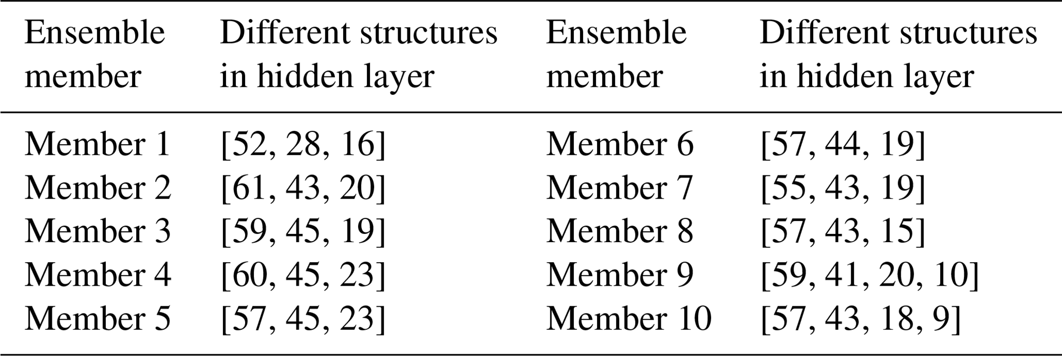
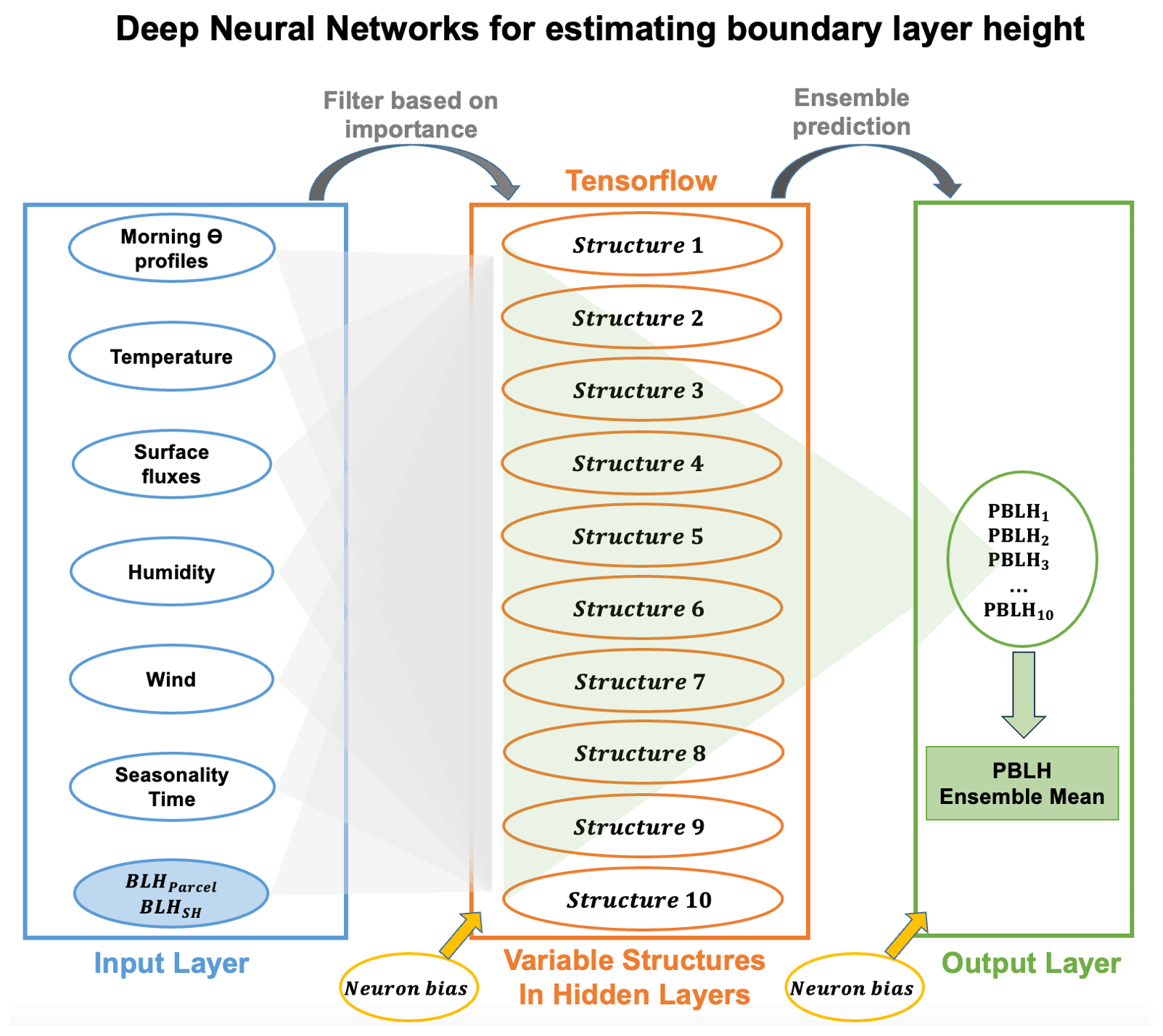
Figure 1 Schematic of the multi-structure deep neural networks (DNNs) used for estimating the planetary boundary layer height (PBLH). Input features, including morning potential temperature profiles, surface air temperature, wind, humidity, surface fluxes, seasonality, and time, are filtered based on importance and fed into the network. The system comprises 10 distinct hidden-layer structures, each processing the inputs to model PBLH. The outputs from these structures are then synthesized to determine the final PBLH value, leveraging the diverse representations of atmospheric properties captured by each neural network configuration. Neuron biases are applied at the output and hidden layers to fine-tune the model's performance.

At the final stage, the model uses the PBLH estimations from different ensembles to get a mean value as the final PBLH retrieval. This process allows the model to leverage the different results of all structures and enhance the generalizability of results. In the DNN model, neuron biases in the output and hidden layers are important for the network's architecture (Battaglia et al., 2018). These biases serve as fine-tuning parameters for adjusting the activation thresholds of neurons in different layers and further refining the model's predictive capabilities. Neuron biases are initialized with small random values at the start of the training process and then iteratively adjusted according to the network weights during the training. Normalization is a preprocessing technique that often leads to improvements in model training by scaling the input features and target values to a standard range (Raju et al., 2020). The normalization process was applied to each input data to ensure that they have a mean of 0 and a standard deviation of 1, as well as the target data. This standardization scales the different input data to a similar range and, thus, contributes a more stable and efficient training process.

The hidden layers of the DNN model incorporate L2 (level 2) regularization to curtail overfitting, while batch normalization aids in stabilizing learning. Moreover, a dropout rate of 0.2 helps the model to generalize better by reducing reliance on any specific neurons during training. We chose the Adam optimizer and mean squared error as the loss function, which aligns with one of the best practices for regression models (Zhang, 2018). The mean absolute error is selected as a metric to evaluate the model's accuracy during the training. We incorporate the early stopping and learning rate reduction callbacks in the model's training for regularization and fine tuning (L. Liu et al., 2019). Such measures ensure optimal performance by terminating training at the right juncture and avoid the overfitting in the final results.

3.2 Training the DNN model

The training of the DNN model was conducted using a PBLH dataset enriched by SONDE and lidar measurements during 1994 to 2016 over the SGP. Table 2 presents the distribution of dataset samples at different hours in local time (defined here as local standard time, UTC−6), which were important for both the training and validation processes of the DNN model. The primary dataset (i.e., PBLH derived from SONDE measurements) is listed in the first column and is available routinely for 05:00, 11:00, and 17:00 LT. The training dataset was augmented with the combined MPL–SONDE PBLH dataset (Su et al., 2020b) and Doppler-lidar-derived PBLH (Sivaraman and Zhang, 2021) to address the gaps where SONDE measurements were not available. In instances where radiosonde data are unavailable, the lidar datasets are used for training, contingent upon their agreement with radiosonde measurements within a margin of 0.2 km over a 3 h window. Specifically, out of the total comparisons during the study period, 40.2 % of the lidar measurements do not agree within the 0.2 km threshold with the SONDE results. The cases with relatively larger inconsistencies stem from various factors, including instrumental errors, rainy conditions, stable PBL conditions, differing definitions, and lidar signal attenuation, as discussed in previous studies (Su et al., 2020b; Kotthaus et al., 2023). These cases were excluded from the DNN model training to maintain the quality of the process.

Table 2 Distribution of dataset samples for deep neural network (DNN) training and validation. This table details the sample data at different hours in local time used for the development and validation of the DNN to estimate the planetary boundary layer height (PBLH). The first column lists the available PBLH values derived from a radiosonde (SONDE; Liu and Liang, 2010) during various hours in local time from 1994 to 2016. The second column supplements the dataset with a combined MPL–SONDE approach (Su et al., 2020b) and Doppler-lidar-derived PBLH (Sivaraman and Zhang, 2021) used in the absence of SONDE measurements; 70 % of the combined dataset from the first and second columns was randomly selected for the model's training. The third column provides the number of SONDE measurements available for validation purposes. Morning SONDE data serve as the input and boundary condition.

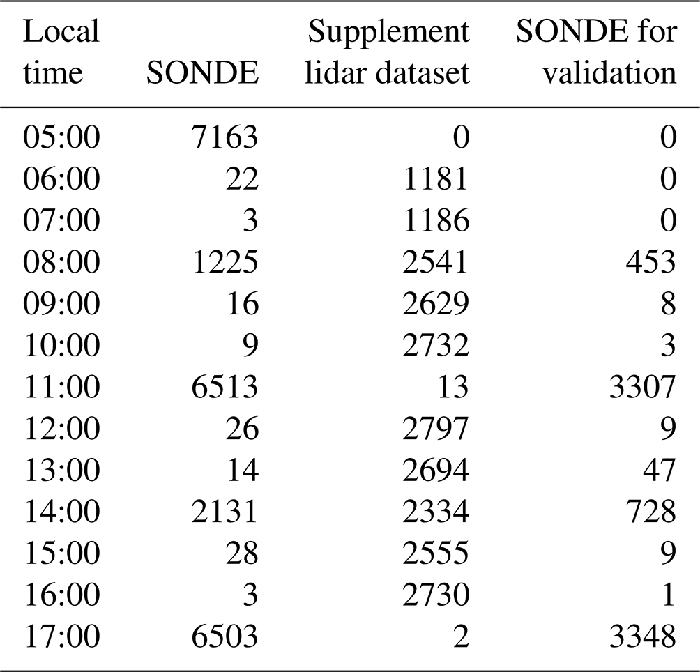
For the purpose of training the DNN model, 70 % of the hourly data from both SONDE measurements and the lidar combined dataset were randomly selected. The dataset of the remaining 30 % comprises the portion of SONDE measurements set aside for validation purposes, including a separate subset from the years 2017 to 2020, to test the model's predictive capabilities on independent data. This training and validation scheme ensures that the DNN model is not only well-trained but also thoroughly evaluated, reinforcing its reliability in accurately estimating PBLH. As morning SONDE data constitute the primary input and boundary conditions for the model, the validation of PBLH retrievals is consequently confined to 08:00 to 18:00 LT.

3.3 Feature importance score

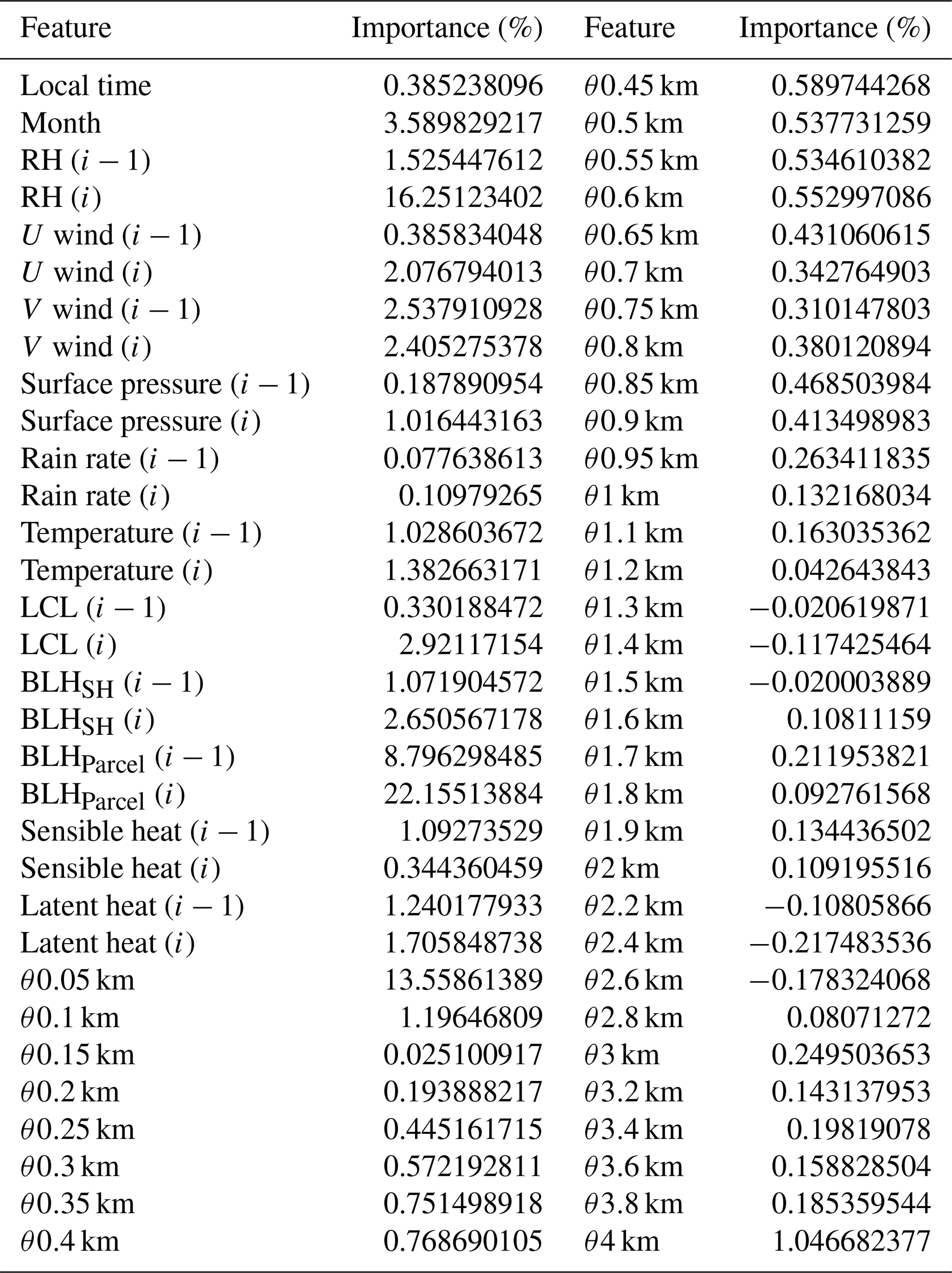
In the DNN model, we quantified the significance of each input parameter using the permutation importance technique, which is a widely used method for deep learning (Date and Kikuchi, 2018; Altmann et al., 2010; Breiman, 2001). Initially, we carried out a test run to determine a baseline performance by calculating the mean absolute error (MAE) on the validation set. Then, each feature within this set was individually shuffled, severing its correlation with the target PBLH, and the MAE was recalculated. Compared to the baseline performance, the increase in MAE from this shuffled state indicates the feature's predictive value: the greater the increase, the more significant the feature. We repeat this shuffling and evaluation 15 times, each with a unique random seed to ensure statistical robustness. Furthermore, we calculated the average MAE increase across these iterations as the importance score. These scores are expressed as percentages, with each feature's importance score normalized to sum to 100 %. Each score quantitatively represents how much the shuffling of a feature increases the MAE, indicating the relative significance of that feature in the model's predictive accuracy and facilitating a straightforward comparison of the influence of each feature within the model. Therefore, we derived a composite importance metric for feature groups to represent their significance as the cumulative sum of related inputs.

Figure 2 presents the importance scores to demonstrate the relative influence of different feature groups on the model's performance. Prominently, BLH_Parcel, morning potential temperature profiles (θ profile), and surface relative humidity are identified as the most important three features, with their substantial impact on the accuracy of PBLH estimation being highlighted. BLH_Parcel is defined as the height where the morning potential temperature first exceeds the current surface potential temperature by more than 1.5 K (Holzworth, 1964; Chu et al., 2019). Among these features, BLH_Parcel captures the response of the PBL to surface heating, which can drastically affect local convection and thus serves as one of the key parameters in the DNN model. Incorporating this parameter and its association with PBL development better simulates diurnal variations in PBLH in the DNN model. Meanwhile, the morning θ profile represents the vertical stratification of thermodynamics and is essential for understanding stability and mixing processes within the PBL. Thus, θ profile serves as the initial boundary condition for the PBLH estimation with a significant importance score. Surface relative humidity also emerges as a key influencer, affecting the model's performance significantly. Humidity levels influence the condensation and evaporation processes within the PBL, which are important in determining its vertical extent layer and structure. Fair-weather and dry conditions are typically associated with a more turbulent and higher PBL. Conversely, high surface humidity often contributes to the formation of boundary layer clouds, which introduces complex interactions with PBL thermodynamics.

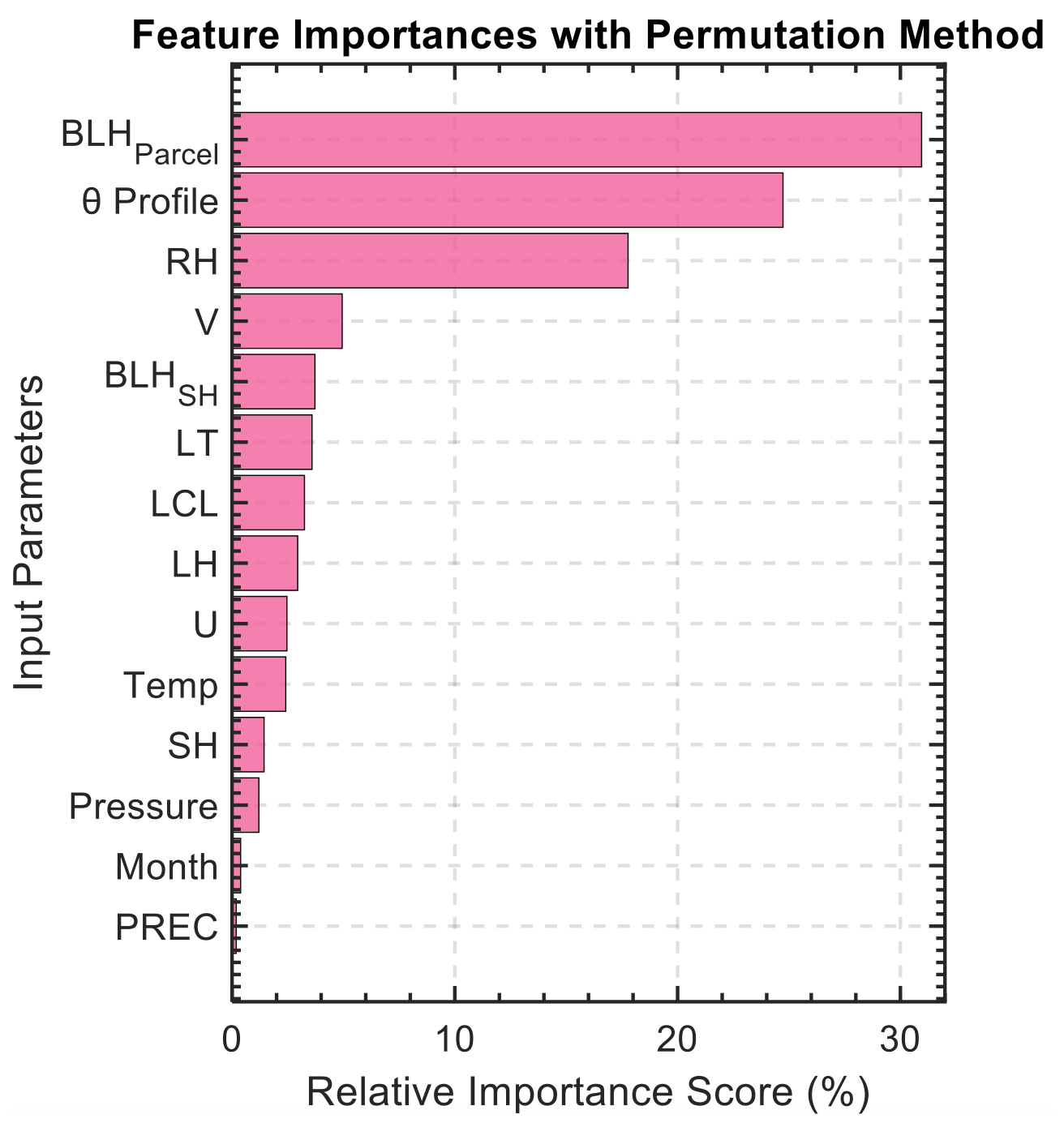
Figure 2 Feature importance with the permutation method in the deep learning model. This table presents the importance scores of each input feature used in the deep learning model to estimate PBLH. The features include the local time (LT), month, relative humidity (RH), surface U and V wind components, pressure at the surface (pressure), precipitation (PREC), surface temperature (temp), sensible and latent heat (SH and LH), surface-derived lifting condensation level (LCL), boundary layer height derived from sensible heat and parcel methods (BLH_Parcel and BLH_SH), and morning profiles of potential temperature (θ profile). The importance scores are presented as percentages, representing each feature's relative contribution to the model's predictive accuracy, normalized to sum to 100 %.

In this analysis, each feature, such as θ profile, comprises several different inputs, and the relative importance scores presented in Fig. 2 are calculated as the cumulative sum of these inputs. Complementing this, Table 3 offers an exhaustive breakdown of importance scores for all considered input features within the deep learning model. In refining the model, features contributing a negligible or negative effect on performance (i.e., importance scores less than 0) are excluded. As a result, this selection criterion has led to the inclusion of 58 out of the original 64 features. This process ensures we only use inputs with a proven positive influence in the DNN model.

Table 3 The relative importance scores (%) of each input feature used in the deep learning model to estimate the planetary boundary layer height. The features include the local time, month, relative humidity, U and V wind components, surface pressure, precipitation, temperature, lifting condensation level (LCL), boundary layer height derived from sensible heat and parcel methods (BLH_SH and BLH_Parcel), sensible and latent heat, and profiles of potential temperature (θ) at different heights. The importance scores are expressed as percentages, indicating each feature's relative contribution to the model's predictive accuracy, normalized to sum to 100 %.

4 Evaluation of the deep learning model

4.1 Comparative analysis of biases among different datasets

A critical component of evaluating our deep learning model's efficacy is analyzing the biases of individual ensemble members and their collective output. Figure 3 offers a visual assessment of the mean absolute error (MAE), root mean square error (RMSE), and correlation coefficient (R) for each ensemble member, alongside a comparison with the ensemble mean (average of all individual ensemble members). The plotted data points reveal the variation in performance across different model architectures, while the ensemble mean, represented by the horizontal dashed lines, indicates the collective accuracy of the ensemble approach. The structures of different hidden-layer configurations are listed in the Table 1.

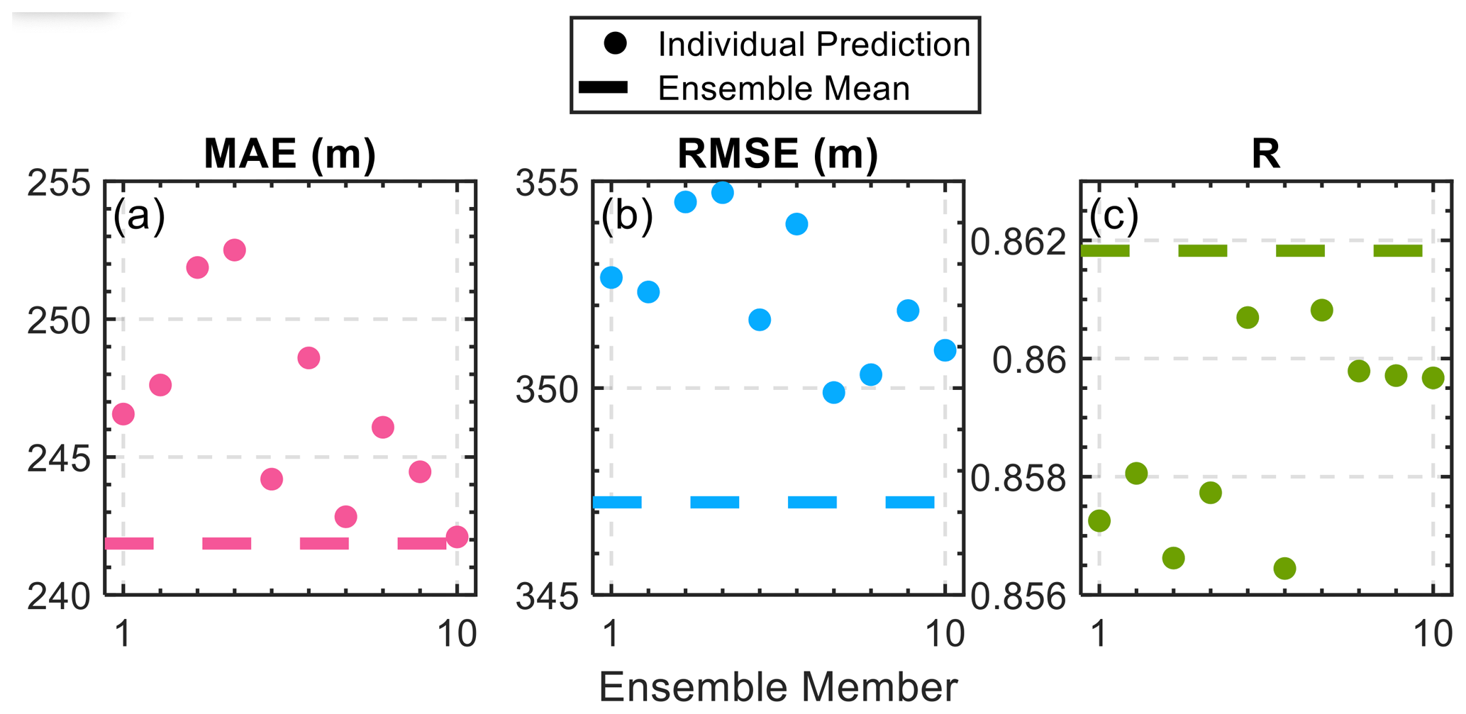
Figure 3 Performance metrics of individual ensemble members and the ensemble mean in estimating the planetary boundary layer height (PBLH). Panel (a) displays the mean absolute error (MAE), panel (b) displays the root mean square error (RMSE), and panel (c) displays the correlation coefficient (R) for each of the 10 ensemble members (represented by dots) and the ensemble mean (indicated by the horizontal dashed line). The ensemble approach demonstrates improved accuracy and reliability in PBLH estimation as evidenced by the aggregation of individual model predictions into a robust ensemble mean.

This methodological consolidation results in a more reliable and accurate PBLH estimation, leveraging the strengths and mitigating the weaknesses of individual models. By integrating multiple neural network configurations, we revealed that an ensemble prediction consistently outperforms the individual models. This strategy can improve the MAE by up to 4.4 %, rendering the model less dependent on any specific structural configuration.

An in-depth comparative analysis of biases among various PBLH estimation methods is essential for validating the reliability and accuracy of the DNN developed in this study. Figure 4 illustrates the MAE trends for several methods over a multi-year span, with SONDE-derived PBLH serving as the benchmark for the ground truth. The analysis reveals the performance of different methodologies: the DNN approach, Doppler lidar, ceilometer, MPL, and Raman lidar. Significantly, the DNN model, depicted in black, maintains a consistent MAE trend throughout the trained period (1994–2016) as well as the subsequent untrained period (2017–2020), demonstrating robust predictive stability. In contrast, the remote-sensing-based methods show a reduction in bias from 2010 to 2022, possibly due to the improvement of remote sensing data quality. The discrepancy in PBLH estimates between the DNN and SONDE remains consistently lower than those observed with conventional remote sensing techniques.

Figure 5 provides a detailed evaluation of the DNN model in comparison to ceilometer- and Doppler-lidar-derived PBLH, as these two methods have demonstrated the high quality with more than 9 years of datasets. Figure 5a–b contrast the PBLH predictions from the DNN model for both the trained period (1994–2016) and untrained period (2017–2020), respectively, showcasing strong correlations and low MAEs, indicative of the model's robust training and generalization capabilities. Figure 5c–d further this examination with ceilometer and Doppler lidar comparisons, respectively. Overall, Doppler lidar exhibits a closer alignment with SONDE-derived PBLH than the ceilometer. However, the MAE from Doppler-lidar-based estimates is still approximately 48 % higher than that derived from the DNN model. The correlation coefficient for the DNN-derived PBLH estimates has seen a substantial improvement, rising from the 0.5–0.6 range typically observed with remote-sensing-based PBLH methods to exceeding 0.8 when compared to SONDE-derived PBLH measurements. This comparative analysis not only confirms the DNN model's accuracy but also offers insights into the relative performance of various contemporary PBLH estimation methodologies.

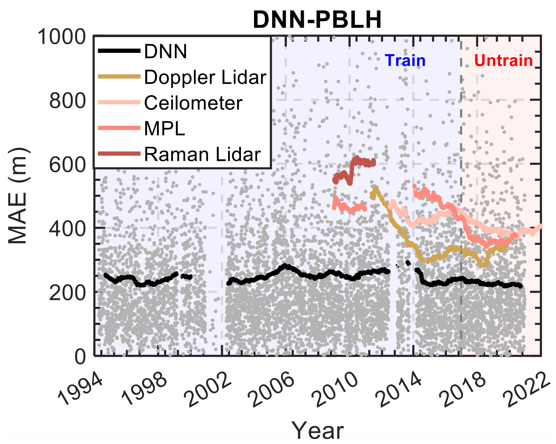
Figure 4 Comparative analysis of the mean absolute error (MAE) in PBLH estimation using different methodologies. PBLH derived from SONDE is considered the ground truth. The DNN approach is shown in black, Doppler lidar data (Sivaraman and Zhang, 2021) are shown in yellow, ceilometer data (Zhang et al., 2022) are shown in pink, micro-pulse lidar data (MPL; Sawyer and Li, 2013) are shown in light red, and Raman lidar data (Ferrare, 2012) are shown in dark red. The DNN model is trained during 1994–2016. Individual MAE values for the DNN are represented by gray dots, while the solid lines denote the smoothed MAE for each method with a 2-year smooth window.

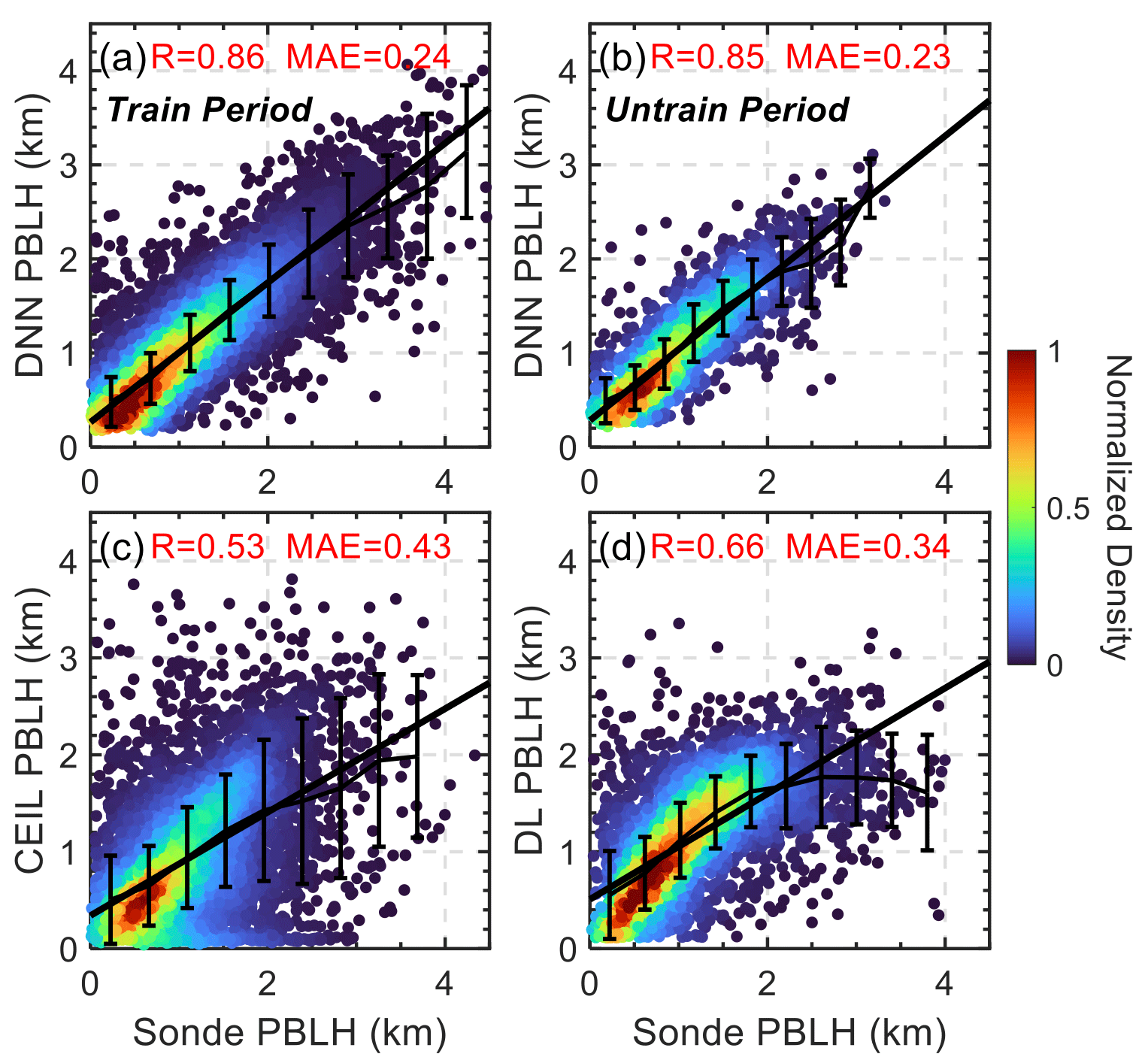
Figure 5 Scatterplots comparing the observed radiosonde (SONDE) PBLH with estimates from the deep learning model and lidar observations. Panels (a) and (b) show PBLH estimated by the deep neural network (DNN) during the trained period (1994–2016) and the untrained period (2017–2020), respectively, with the corresponding correlation coefficient (R) and mean absolute error (MAE). Panels (c) and (d) display comparisons of SONDE PBLH with the ceilometer-derived (CEIL) and Doppler-lidar-derived (DL) PBLH, respectively. The color gradient indicates the normalized density of data points, while the solid black line represents the line of best fit and error bars indicate the mean and standard deviations for each bin.

4.2 Performances of PBLH retrievals under different conditions

The performance of PBLH retrievals under varying atmospheric conditions is a crucial aspect of model evaluation. In Fig. 6, the seasonal diurnal cycles of PBLH estimated by different methods are presented, offering information into the diurnal and seasonal evolution of PBLH. As PBLH demonstrates notable variations for different seasons and hours in local time with large differences between summer and winter, the DNN and Doppler lidar estimates show good agreement and closely track the variations observed in SONDE data. Meanwhile, the ceilometer presents an underestimation of PBLH, especially for the summer afternoon, indicating the potential bias of ceilometer-derived PBLH under a convective environment.

Figure 7 illustrates the diurnal variation in the model's performance by comparing the correlation coefficient, RMSE, and MAE against SONDE-derived PBLH as the reference. The bar graphs for each hour in local time offer a comparison of the RMSE and MAE, as well as the correlation, showcasing the model's precision and consistency relative to remote sensing methods (i.e., ceilometer and Doppler lidar). Ceilometer-derived PBLH exhibits the greatest variations during different hours, particularly around noon, suggesting a time-dependent bias in its measurements. Conversely, both the DNN and Doppler-lidar-derived PBLH demonstrate stable performance in terms of MAE and RMSE throughout the day. Regarding the correlation, remote sensing methods like the use of ceilometer and Doppler lidar measurements exhibit a lower correlation with SONDE-derived PBLH, especially in the early hours (08:00–09:00 LT) with a value of 0.1–0.3, indicating potential limitations in their reliability during these times. On the other hand, the DNN model shows a relatively good correlation with SONDE retrievals (above 0.6 under different hours). This comparison shows the efficacy of the DNN in tracking the diurnal cycle of PBLH.

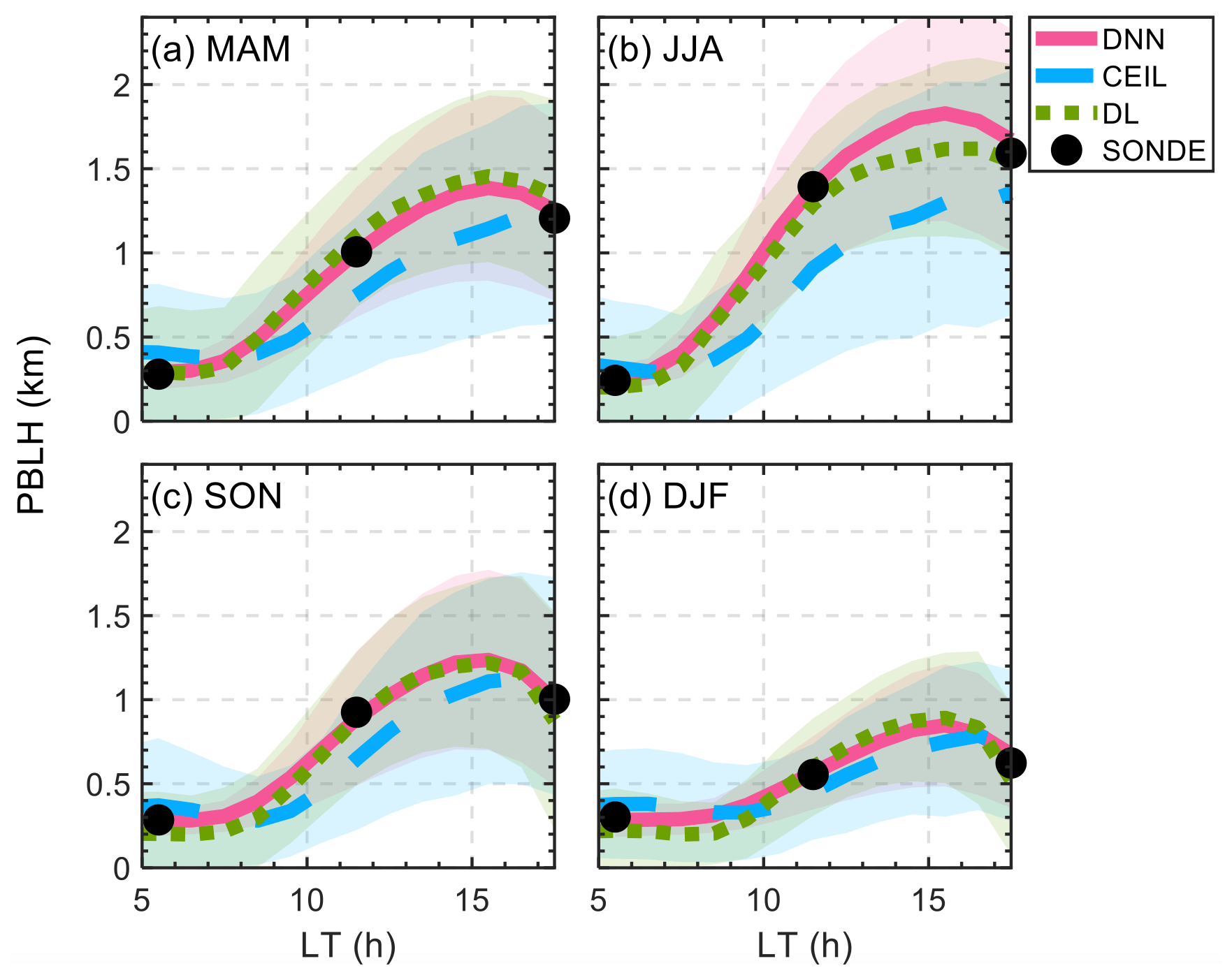
Figure 6 Seasonally averaged daytime evolution of the planetary boundary layer height (PBLH) derived from various methods. The panels represent the mean PBLH values throughout the day for different seasons: (a) March–April–May (MAM), (b) June–July–August (JJA), (c) September–October–November (SON), and (d) December–January–February (DJF). The PBLH values estimated by the deep neural network (DNN) are shown in red, ceilometer-derived (CEIL) estimates are in blue, Doppler-lidar-derived (DL) estimates are in green, and observed radiosonde (SONDE) data are in black. Shaded areas around the lines indicate the standard deviations within each method.

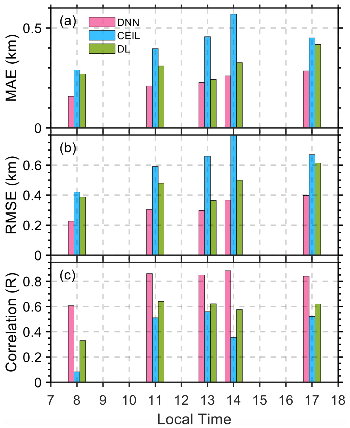
Figure 7 Diurnal variations in the performance metrics for estimating PBLH using different datasets. Panel (a) shows the correlation coefficient (R), panel (b) represents the root mean square error (RMSE), and panel (c) depicts the mean absolute error (MAE) at various local times throughout the day. The deep neural network (DNN) estimates are in blue, ceilometer-derived (CEIL) estimates are in pink, and Doppler-lidar-derived (DL) estimates are in green. Note that these bias metrics are calculated using SONDE PBLH as the standard. The availability of SONDE data for different hours is detailed in Table 2.

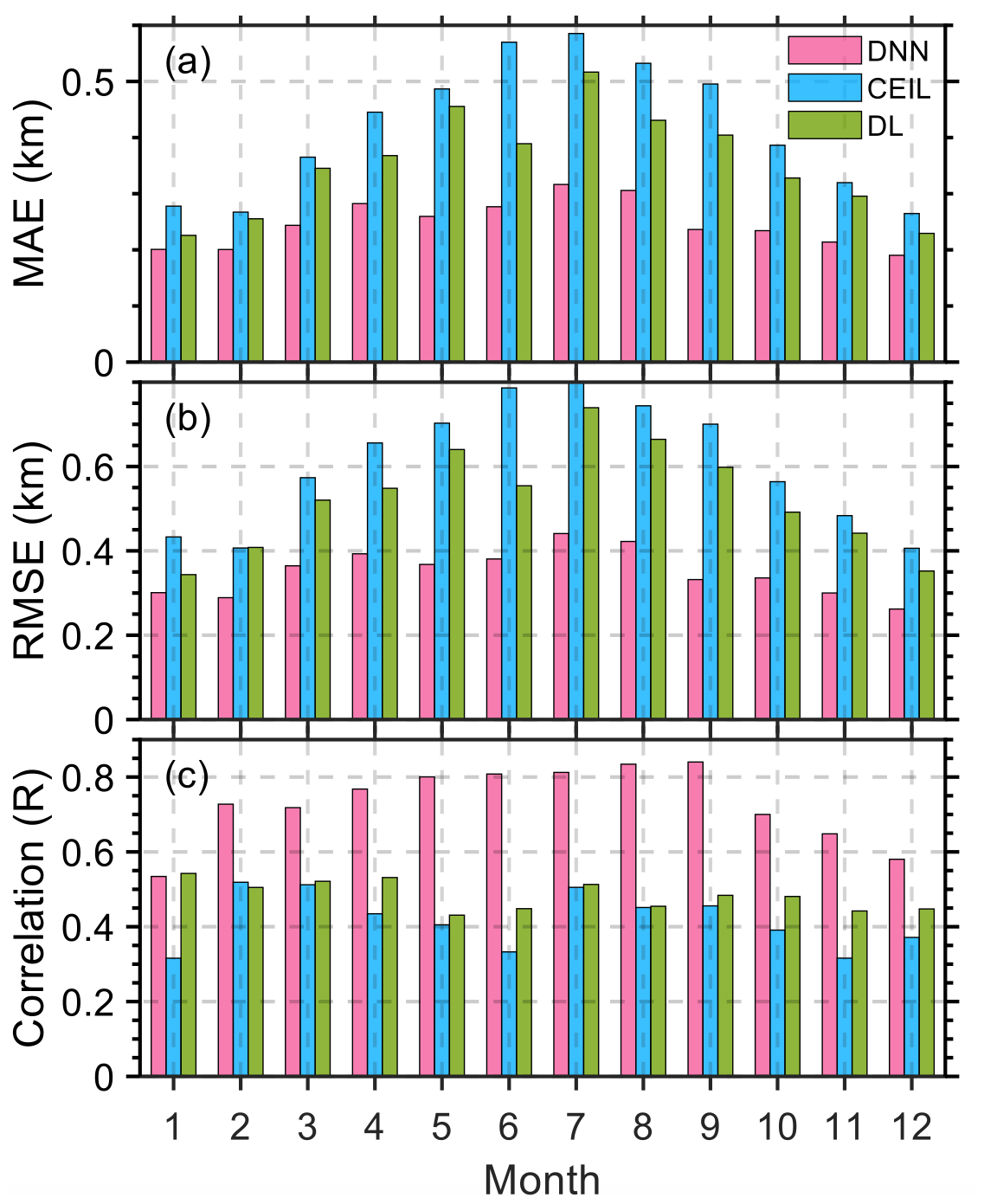
Continuing our assessment of the DNN model, we analyze the DNN model's monthly performance in estimating PBLH, as shown in Fig. 8. The analysis compares MAE, RMSE, and correlation coefficients for each month to assess the model's precision and dependability. The summer months (June–July–August) exhibit higher biases, with MAE values for the DNN, ceilometer, and Doppler lidar at 0.3, 0.56, and 0.45 km, respectively. In contrast, the winter months (December–January–February) show reduced biases, with MAE values of 0.2 km for the DNN, 0.27 km for the ceilometer, and 0.24 km for the Doppler lidar. Specifically, the DNN model shows a much lower bias during the summer season. Compared to the remote-sensing-based retrievals, DNN-derived PBLH shows a much better agreement with SONDE-derived PBLH, increasing from 0.3–0.6 to approximately 0.8 in terms of correlation coefficients.

Figure 9 presents the biases of PBLH retrievals under clear-sky and low-cloud conditions. We calculated biases as the absolute deviation from the mean PBLH for each condition, focusing particularly on the differences between low-cloud (maximum cloud fraction between 0–4 km exceeding 1 %) and clear-sky (total cloud fraction below 1 %) scenarios. The threshold of 1 % for cloud fraction is also used to identify the cloud base height (CBH) in the European Centre for Medium-Range Weather Forecasts' fifth-generation global reanalysis (ERA5; Hersbach et al., 2023). The violin plots in this figure illustrate the data distribution of biases for each method to demonstrate their variability. For the DNN model and ceilometer, the relative biases between clear and cloudy conditions are comparable and the difference is less than 1 %. This suggests a consistent performance across these atmospheric states. However, the Doppler lidar exhibits a larger disparity, showing a 5.5 % bias under cloudy conditions compared to clear skies. Moreover, the spread of biases (shaded areas and error bars) is notably wider for both the ceilometer and Doppler lidar. This indicates large variability in their performance. For all three methods, the mean biases are notably higher than the median values. Such differences indicate that the mean values are notably influenced by outliers under both clear-sky and cloudy conditions.

Figure 8 Similar to Fig. 7 but MAE, RMSE, and R for different months.

The evolution of PBLH under shallow-cumulus conditions offers insights into the interactions between clouds, PBL, and land surface (Zhang and Klein, 2010, 2013). Figure 10 demonstrates the variations in PBLH measurements from different methods during conditions typical of shallow cumulus clouds. Shallow cumulus clouds were identified following Su et al. (2024b). Specifically, these coupled clouds form post-sunrise, and the sky must not be overcast, characterized by a cloud fraction less than 90 %. This selection criterion ensures that the observed cloud formations are primarily driven by surface heating and local convection. The DNN model closely matches SONDE-derived PBLH and the CBH from ARSCL. This alignment underscores the physical validity of the DNN approach, confirming its capability to replicate traditional measurement techniques to a good extent of accuracy. Meanwhile, Doppler-lidar-derived PBLH retrievals also show high consistency with SONDE measurements, whereas ceilometer-derived PBLH generally underestimates values under shallow-cumulus conditions.

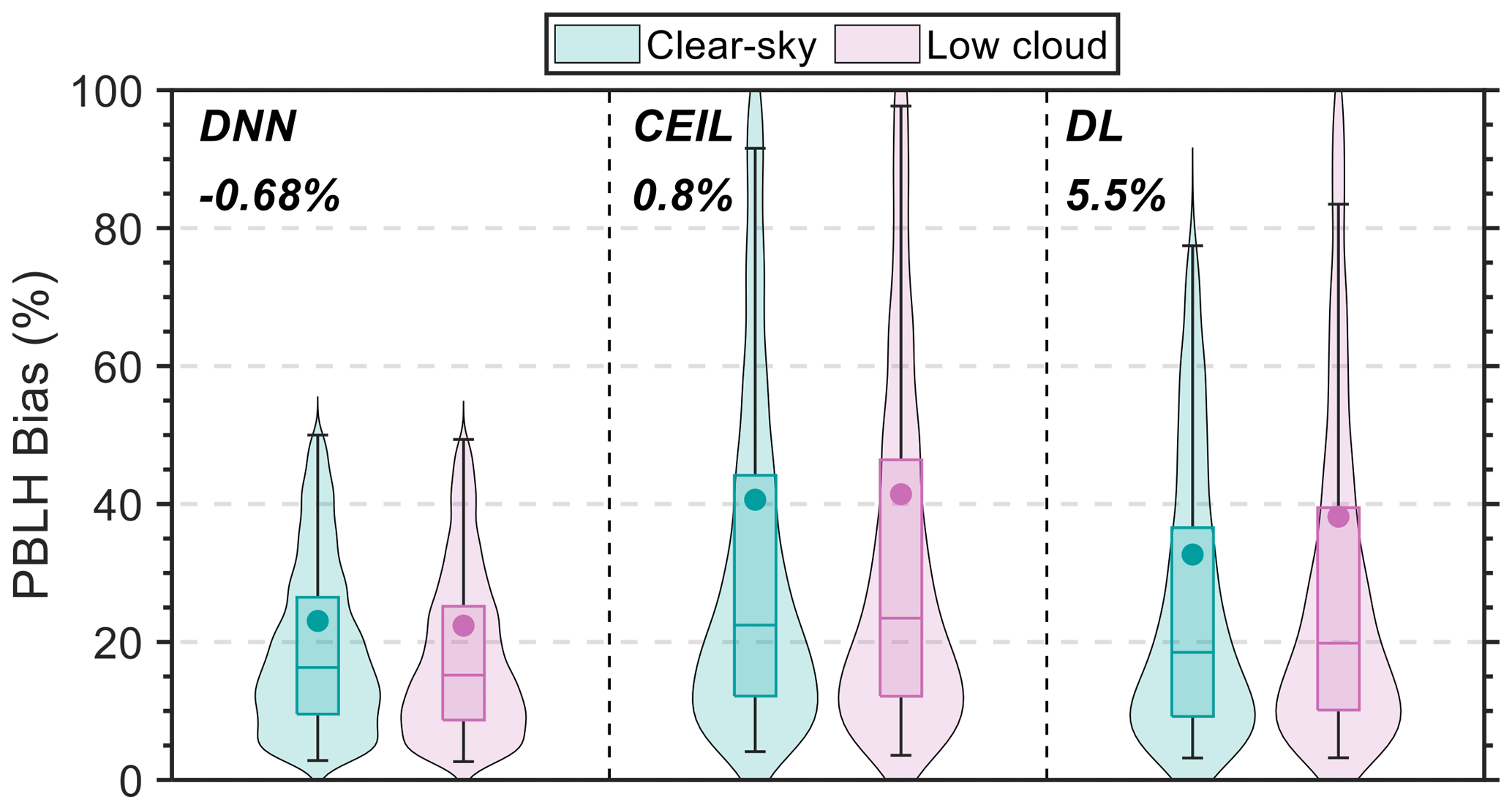
Figure 9 Comparative analysis of PBLH estimation bias under clear-sky and low-cloud conditions for various methods. Bias percentages are computed as the absolute bias normalized by the mean PBLH for each condition, with the number above each method indicating the difference in mean bias between low-cloud and clear-sky scenarios. The boxplots detail the 10th, 25th, 50th, 75th, and 90th percentiles, while shaded areas in violin plots illustrate the distribution of dataset biases. The dots indicate the mean value for each condition.

Figure 10 also demonstrates the general relationship between the development of shallow cumulus clouds and the PBL, which is driven by local convection and turbulence. The formation of these cumulus clouds is linked to rising thermals and an increase in surface heat fluxes, essential for driving vertical mixing within the sub-cloud layer. This relationship is evidenced by the increased occurrence of cumulus clouds along with an increase in DNN-derived PBLH from morning to late afternoon. Specifically, during periods with a high frequency of shallow cumulus clouds, DNN-derived PBLH often surpasses the CBH. This indicates that rising air parcels extend beyond the condensation level, facilitating the formation and development of coupled cumulus clouds.

In this context, these analyses confirm the physical consistency of DNN-derived PBLH with traditional measurement techniques and highlight its physically reasonable variations during cloudy conditions. The results presented in this section illustrate the effectiveness of the DNN model in capturing the PBLH variations across different hours in local time, seasons, and cloudy conditions. Compared to traditional remote sensing methods, the DNN model exhibits relatively good accuracy in aligning with SONDE-derived PBLH, indicating its capability and stable performance under different scenarios.

4.3 Testing the DNN model's adaptability

The DNN model relies on the incorporation of morning temperature profiles as inputs, such as detailed in Table 3. This dependency prompts the question of how to proceed the DNN model in the absence of SONDE data at specific locations. As a solution, we suggest employing morning temperature profiles from the ERA5 (Hersbach et al., 2020) dataset when radiosonde data are not available to maintain the model's operational integrity for the conditions without SONDE data. As one of the most advanced reanalysis datasets, ERA5 is generated by the Integrated Forecasting System coupled with a data assimilation system and offers the meteorological data at a spatial resolution of 0.25° × 0.25°.

Figure 11 assesses the performance of the DNN produced by multi-source field observations in estimating PBLH using morning temperature profiles from ERA5 (05:00 LT) and observed surface meteorological data. The temperature profiles in ERA5 have a vertical resolution of 25 hPa in the lower atmosphere and are interpolated into different levels described in Table 3. By utilizing ERA5 morning profiles, the model demonstrates performance similar to those results achieved with radiosonde inputs, as evidenced by comparing Figs. 11a and 5. Moreover, this alternative approach also shows enhanced accuracy over the native PBLH model outputs from ERA5, increasing the correlation coefficient from 0.74 to 0.86 and reducing the MAE from 0.3 to 0.25 km. In addition, it is important to acknowledge that the PBLH represented in ERA5 is indicative of a grid-average value, approximately 25 km in scale, and therefore inherently differs from site-specific data.

Figure 10 Daytime evolution of the planetary boundary layer height (PBLH) derived from various methods under the shallow-cumulus condition. PBLH values estimated by the deep neural network (DNN) are shown in red, ceilometer-derived (CEIL) estimates are in blue, and Doppler-lidar-derived (DL) estimates are in green. Observed radiosonde (SONDE) data are represented by black stars. Purple bars show the relative frequency of shallow-cumulus occurrences throughout the day, while purple dots mark the corresponding cloud base height (CBH). Shaded areas around each line reflect the standard deviations for each method.

Figure 11 Scatterplots comparing SONDE PBLH with estimates from the DNN and ERA5. (a) The comparison between observed SONDE PBLH and estimates from the DNN model, which utilizes morning temperature profiles (05:00 LT) from ERA5 (ERA profile) and observed surface meteorological data (surface OBS) as inputs. (b) The correlation comparison of observed SONDE PBLH and PBLH model outputs from the ERA5 datasets. The color gradient in both panels represents the normalized density of data points, while the solid black line indicates the linear regression and the error bars denote the mean and standard deviations for each bin.

These findings highlight the alternative DNN model's robustness, offering a reliable substitute for radiosonde data by leveraging reanalysis data with similar performance. This demonstrates the DNN model's adaptability and potential as a practical tool for PBLH estimation across various meteorological sites, especially in regions or periods where radiosonde data may be lacking.

We further test the adaptability and generalizability of the DNN model by applying it across different climatic and geographic regions. To this end, we extended our model evaluation to include SONDE and surface meteorological data from the GoAmazon (tropical rainforest) and CACTI (middle-latitude mountain) field campaigns. Seasonality is accounted for as an input variable in the DNN model, with months in the Southern Hemisphere adjusted to reflect their Northern Hemisphere seasonal counterparts (e.g., July inputs are treated as January). The normalization process (Sect. 3.1) was reapplied for the CACTI campaign data to adjust for notable pressure level variations, ensuring input standardization with a mean of 0 and unit variance.

Figure 12 presents the model's performance, in comparison to SONDE observations for both the GoAmazon and CACTI campaigns. The DNN model demonstrates commendable adaptability, maintaining a strong correlation (0.86–0.88) with SONDE measurements (Fig. 12a–b). Further comparison is provided, which assesses the performance of ceilometer-derived PBLH against SONDE measurements for the same campaigns. When assessing the performance of ceilometer-derived PBLH against SONDE measurements for the same campaigns, the DNN model exhibited both stronger correlations and smaller biases, as shown in Fig. 12b–d.

Figure 12 Validation of the DNN trained over the SGP for the GoAmazon (tropical rainforest) and CACTI (middle-latitude mountain) field campaigns. Panels (a) and (c) illustrate the correlation (R) and mean absolute error (MAE) between DNN predictions and SONDE observations for GoAmazon and CACTI, respectively. Panels (b) and (d) show the performance of ceilometer-derived (CEIL) PBLH compared to SONDE for the same campaigns. The color gradient indicates the normalized density of data points, while the solid black line represents the line of best fit and error bars indicates the mean and standard deviations for each bin.

Nevertheless, the analysis highlighted the presence of systematic biases, with relatively larger MAE at the GoAmazon and CACTI sites compared to the SGP site. Figure 13 underscores this by presenting a comparative analysis of PBLH means and standard deviations across the three ARM sites. The early morning measurements during 05:00–07:00 LT are excluded. The results, derived from the DNN model and SONDE, ceilometer, and Doppler lidar data, reveal average differences in PBLH means relative to SONDE measurements. These differences suggest an overestimation (+15 %) and underestimation (−23 %) by the DNN model for the GoAmazon and CACTI sites, respectively, compared to the more consistent PBLH values at the SGP site.

The evident systematic deviations when applying the SGP-trained DNN model to the diverse environments of GoAmazon and CACTI underscore the challenges in generalizing the model to regions with significantly different meteorological backgrounds. These findings point to the potential of DNN models for PBLH estimation while also highlighting the necessity for region-specific model adjustments.

Figure 13 Comparative PBLH mean (dots) and standard deviations (error bars) across ARM sites (SGP, GoAmazon, and CACTI). The datasets are derived from radiosonde data (SONDE; in black), the DNN model (in pink), ceilometer data (CEIL; in blue), and Doppler lidar data (DL; in green), respectively. Note that DL-derived PBLH is only available at the SGP. The percentages in various colors denote the differences in PBLH means derived from the DNN, CEIL, and DL methods relative to SONDE observations. To mitigate sampling bias, these mean values and standard deviations are computed exclusively for intervals where all instruments have concurrently available data.

5 Summary

This study has developed a multi-structure DNN model for estimating PBLH using conventional meteorological data. The DNN model is developed by leveraging a long-term dataset of PBLH derived from radiosonde data and augmented with high-resolution MPL and Doppler lidar observations. This model produced a PBLH dataset over the SGP with robust accuracy, consistently yielding lower bias values across various conditions and datasets. Utilizing conventional meteorological data, this method generates a 27-year dataset over the SGP, encompassing periods with limited remote sensing data availability. In situations where morning radiosonde data are unavailable, ERA5 data can be effectively employed to initiate the model, offering a practical alternative.

An important aspect of this research involved comparing DNN models with diverse remote sensing instruments. Although these instruments offer high temporal and vertical resolution, discrepancies in PBLH estimation remain. Our DNN model, leveraging a broad range of input features refined by their importance, constructs a representation of PBL evolutions, frequently demonstrating a closer agreement with SONDE-derived PBLH. In the absence of remote sensing data, the DNN model can produce high-quality PBLH estimates from the conventional meteorology data.

The study has shown the DNN model's ability to synthesize complex patterns from meteorological data, reflecting the versatility of machine learning in simulating the boundary layer processes. Its application to varied geographic terrains and climates during the GoAmazon and CACTI campaigns has further validated its adaptability, demonstrating a high correlation between DNN-derived PBLH and SONDE-derived PBLH. Nonetheless, systematic biases in regions outside the SGP highlight the influence of regional factors in PBLH estimation and suggest the need for region-specific refinements to the model.

In summary, this research introduces a machine learning framework for PBLH estimation that is able to generate high-quality PBLH using meteorological data, independent of remote sensing instruments. This methodology, alongside the datasets derived from the deep learning model, is beneficial in advancing our understanding of PBL daytime development including thermodynamics and dynamics. It also has implications for improved representation of the PBL processes in weather forecasting and climate models, particularly by offering the potential to diagnose PBL in models through the integration of modeled meteorological data as input. Future efforts will be directed towards refining this model to ensure its wide applicability over a global scale. These developments aim to effectively tackle the challenges of systematic biases and regional variability in PBLH estimation.